ieee transactions on industrial informatics …wilambm/pap/2012/tii-pukish-2187914-x.pdf · ieee...

IEEE TRANSACTIONS ON INDUSTRIAL INFORMATICS 1

Selection of Proper Neural Network Sizes andArchitectures—A Comparative Study

David Hunter, Hao Yu, Student Member, IEEE, Michael S. Pukish, III, Student Member, IEEE, Janusz Kolbusz, andBogdan M. Wilamowski, Fellow, IEEE

Abstract—One of the major difficulties facing researchers usingneural networks is the selection of the proper size and topologyof the networks. The problem is even more complex because oftenwhen the neural network is trained to very small errors, it may notrespond properly for patterns not used in the training process. Apartial solution proposed to this problem is to use the least possiblenumber of neurons along with a large number of training patterns.

The discussion consists of three main parts: first, differentlearning algorithms, including the Error Back Propagation (EBP)algorithm, the Levenberg Marquardt (LM) algorithm, and therecently developed Neuron-by-Neuron (NBN) algorithm, arediscussed and compared based on several benchmark problems;second, the efficiency of different network topologies, includingtraditional Multilayer Perceptron (MLP) networks, BridgedMultilayer Perceptron (BMLP) networks, and Fully ConnectedCascade (FCC) networks, are evaluated by both theoretical anal-ysis and experimental results; third, the generalization issue isdiscussed to illustrate the importance of choosing the proper sizeof neural networks.

Index Terms—Architectures, learning algorithms, neural net-works, topologies.

I. INTRODUCTION

N EURAL networks are currently used in many dailylife applications. In 2007, a special issue of TIE was

published only on their application in industrial practice [1].Further applications of neural networks continue in variousareas. Neural networks are used for controlling induction mo-tors [2]–[4] and permanent magnet motors [5]–[7], includingstepper motors [8]. They are also used in controlling other dy-namic systems [9]–[16], including robotics [17], motion control[18], and harmonic distortion [19], [20]. They are also usedin industrial job-shop-scheduling [21], networking [22], andbattery control [23]. Neural networks can also easily simulatehighly complex dynamic systems such as oil wells [24] whichare described by more than 25 nonlinear differential equations.Neural networks have already been successfully implementedin embedded hardware [25]–[29].

People who are trying to use neural networks in their researchare facing several questions.

Manuscript received October 02, 2011; revised January 23, 2012; acceptedJanuary 31, 2012. Date of publication February 14, 2012; date of current versionnulldate. Paper no. TII-12-0052.

D. Hunter, H. Yu, M. S. Pukish, and B. M. Wilamowski are with the De-partment of Electrical and Computer Engineering, Auburn University, Auburn,AL 36849-5201 USA (e-mail: [email protected]; [email protected]; [email protected]; [email protected]).

J. Kolbusz is with the Department of Distributed Systems, University of In-formation Technology and Management, Rzeszow 35-225, Poland (e-mail: [email protected]).

Digital Object Identifier 10.1109/TII.2012.2187914

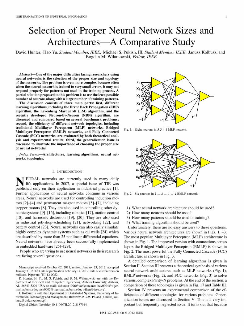
Fig. 1. Eight neurons in 5-3-4-1 MLP network.

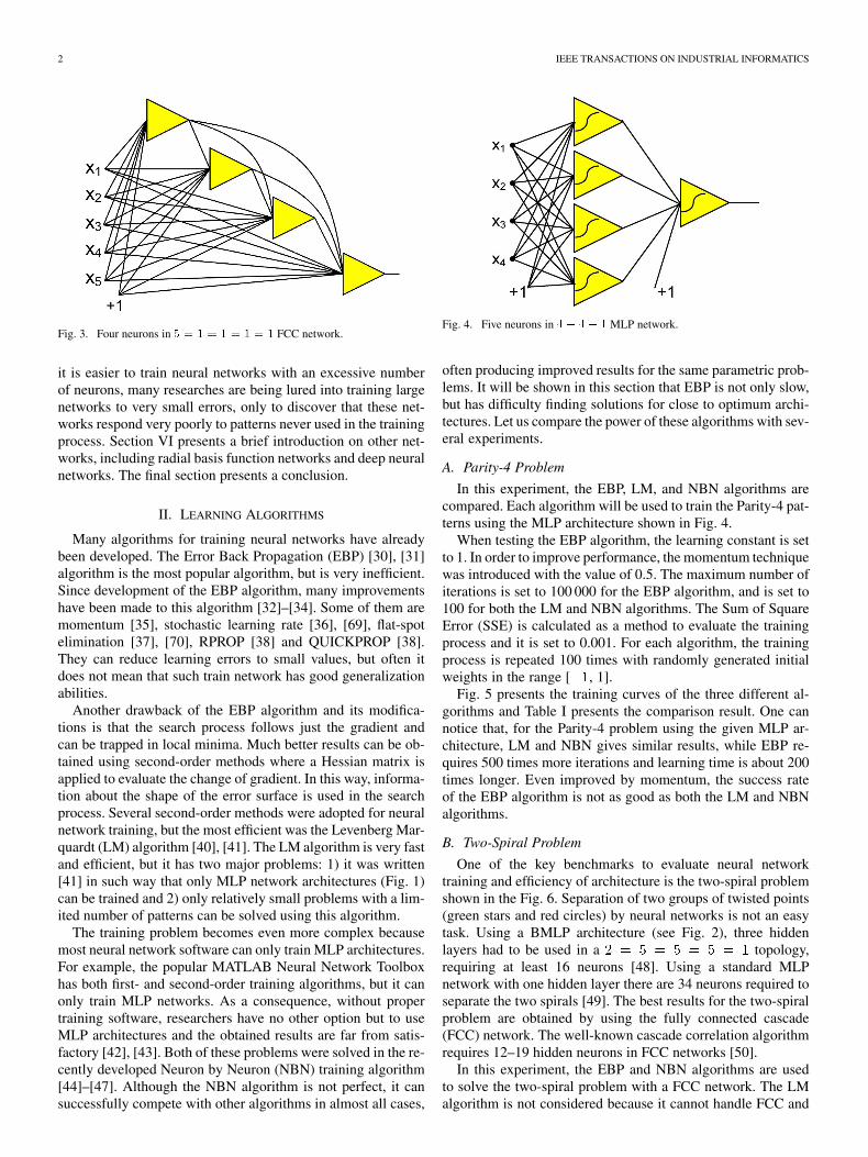
Fig. 2. Six neurons in � � � � � � � BMLP network.

1) What neural network architecture should be used?2) How many neurons should be used?3) How many patterns should be used in training?4) What training algorithm should be used?Unfortunately, there are no easy answers to these questions.

Various neural network architectures are shown in Figs. 1, –3.The most popular, Multilayer Perceptron (MLP) architecture isshown in Fig. 1. The improved version with connections acrosslayers the Bridged Multilayer Perceptron (BMLP) is shown inFig. 2. The most powerful the Fully Connected Cascade (FCC)architecture is shown in Fig. 3.

A detailed comparison of learning algorithms is given inSection II. Section III presents a theoretical synthesis of variousneural network architectures such as MLP networks (Fig. 1),BMLP networks (Fig. 2), and FCC networks (Fig. 3) to solvevarious, complex Parity-N problems. At the end of the section, acomparison of these topologies is given in Fig. 17 and Table III.

Section IV presents an experimental comparison of the ef-ficiencies of different topologies for various problems. Gener-alization issues are discussed in Section V. This is a very im-portant but frequently neglected issue. It turns out that because

1551-3203/$31.00 © 2012 IEEE

2 IEEE TRANSACTIONS ON INDUSTRIAL INFORMATICS

Fig. 3. Four neurons in � � � � � � � � � FCC network.

it is easier to train neural networks with an excessive numberof neurons, many researches are being lured into training largenetworks to very small errors, only to discover that these net-works respond very poorly to patterns never used in the trainingprocess. Section VI presents a brief introduction on other net-works, including radial basis function networks and deep neuralnetworks. The final section presents a conclusion.

II. LEARNING ALGORITHMS

Many algorithms for training neural networks have alreadybeen developed. The Error Back Propagation (EBP) [30], [31]algorithm is the most popular algorithm, but is very inefficient.Since development of the EBP algorithm, many improvementshave been made to this algorithm [32]–[34]. Some of them aremomentum [35], stochastic learning rate [36], [69], flat-spotelimination [37], [70], RPROP [38] and QUICKPROP [38].They can reduce learning errors to small values, but often itdoes not mean that such train network has good generalizationabilities.

Another drawback of the EBP algorithm and its modifica-tions is that the search process follows just the gradient andcan be trapped in local minima. Much better results can be ob-tained using second-order methods where a Hessian matrix isapplied to evaluate the change of gradient. In this way, informa-tion about the shape of the error surface is used in the searchprocess. Several second-order methods were adopted for neuralnetwork training, but the most efficient was the Levenberg Mar-quardt (LM) algorithm [40], [41]. The LM algorithm is very fastand efficient, but it has two major problems: 1) it was written[41] in such way that only MLP network architectures (Fig. 1)can be trained and 2) only relatively small problems with a lim-ited number of patterns can be solved using this algorithm.

The training problem becomes even more complex becausemost neural network software can only train MLP architectures.For example, the popular MATLAB Neural Network Toolboxhas both first- and second-order training algorithms, but it canonly train MLP networks. As a consequence, without propertraining software, researchers have no other option but to useMLP architectures and the obtained results are far from satis-factory [42], [43]. Both of these problems were solved in the re-cently developed Neuron by Neuron (NBN) training algorithm[44]–[47]. Although the NBN algorithm is not perfect, it cansuccessfully compete with other algorithms in almost all cases,

Fig. 4. Five neurons in �� MLP network.

often producing improved results for the same parametric prob-lems. It will be shown in this section that EBP is not only slow,but has difficulty finding solutions for close to optimum archi-tectures. Let us compare the power of these algorithms with sev-eral experiments.

A. Parity-4 Problem

In this experiment, the EBP, LM, and NBN algorithms arecompared. Each algorithm will be used to train the Parity-4 pat-terns using the MLP architecture shown in Fig. 4.

When testing the EBP algorithm, the learning constant is setto 1. In order to improve performance, the momentum techniquewas introduced with the value of 0.5. The maximum number ofiterations is set to 100 000 for the EBP algorithm, and is set to100 for both the LM and NBN algorithms. The Sum of SquareError (SSE) is calculated as a method to evaluate the trainingprocess and it is set to 0.001. For each algorithm, the trainingprocess is repeated 100 times with randomly generated initialweights in the range [ , 1].

Fig. 5 presents the training curves of the three different al-gorithms and Table I presents the comparison result. One cannotice that, for the Parity-4 problem using the given MLP ar-chitecture, LM and NBN gives similar results, while EBP re-quires 500 times more iterations and learning time is about 200times longer. Even improved by momentum, the success rateof the EBP algorithm is not as good as both the LM and NBNalgorithms.

B. Two-Spiral Problem

One of the key benchmarks to evaluate neural networktraining and efficiency of architecture is the two-spiral problemshown in the Fig. 6. Separation of two groups of twisted points(green stars and red circles) by neural networks is not an easytask. Using a BMLP architecture (see Fig. 2), three hiddenlayers had to be used in a topology,requiring at least 16 neurons [48]. Using a standard MLPnetwork with one hidden layer there are 34 neurons required toseparate the two spirals [49]. The best results for the two-spiralproblem are obtained by using the fully connected cascade(FCC) network. The well-known cascade correlation algorithmrequires 12–19 hidden neurons in FCC networks [50].

In this experiment, the EBP and NBN algorithms are usedto solve the two-spiral problem with a FCC network. The LMalgorithm is not considered because it cannot handle FCC and

HUNTER et al.: SELECTION OF PROPER NEURAL NETWORK SIZES AND ARCHITECTURES—A COMPARATIVE STUDY 3

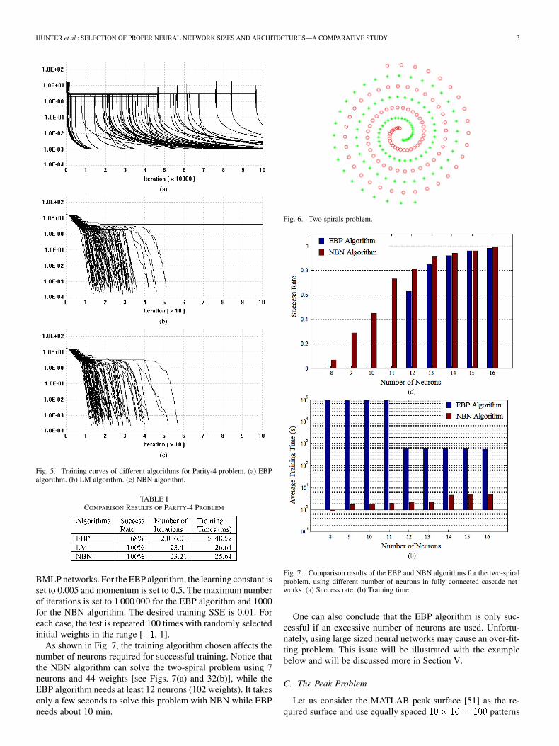
Fig. 5. Training curves of different algorithms for Parity-4 problem. (a) EBPalgorithm. (b) LM algorithm. (c) NBN algorithm.

TABLE ICOMPARISON RESULTS OF PARITY-4 PROBLEM

BMLP networks. For the EBP algorithm, the learning constant isset to 0.005 and momentum is set to 0.5. The maximum numberof iterations is set to 1 000 000 for the EBP algorithm and 1000for the NBN algorithm. The desired training SSE is 0.01. Foreach case, the test is repeated 100 times with randomly selectedinitial weights in the range [ , 1].

As shown in Fig. 7, the training algorithm chosen affects thenumber of neurons required for successful training. Notice thatthe NBN algorithm can solve the two-spiral problem using 7neurons and 44 weights [see Figs. 7(a) and 32(b)], while theEBP algorithm needs at least 12 neurons (102 weights). It takesonly a few seconds to solve this problem with NBN while EBPneeds about 10 min.

Fig. 6. Two spirals problem.

Fig. 7. Comparison results of the EBP and NBN algorithms for the two-spiralproblem, using different number of neurons in fully connected cascade net-works. (a) Success rate. (b) Training time.

One can also conclude that the EBP algorithm is only suc-cessful if an excessive number of neurons are used. Unfortu-nately, using large sized neural networks may cause an over-fit-ting problem. This issue will be illustrated with the examplebelow and will be discussed more in Section V.

C. The Peak Problem

Let us consider the MATLAB peak surface [51] as the re-quired surface and use equally spaced patterns


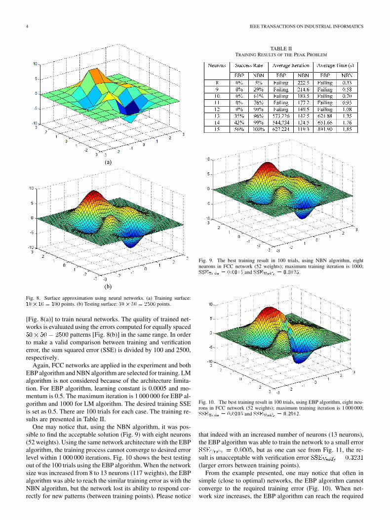
Fig. 8. Surface approximation using neural networks. (a) Training surface:�� points. (b) Testing surface: �� points.

[Fig. 8(a)] to train neural networks. The quality of trained net-works is evaluated using the errors computed for equally spaced

patterns [Fig. 8(b)] in the same range. In orderto make a valid comparison between training and verificationerror, the sum squared error (SSE) is divided by 100 and 2500,respectively.

Again, FCC networks are applied in the experiment and bothEBP algorithm and NBN algorithm are selected for training. LMalgorithm is not considered because of the architecture limita-tion. For EBP algorithm, learning constant is 0.0005 and mo-mentum is 0.5. The maximum iteration is 1 000 000 for EBP al-gorithm and 1000 for LM algorithm. The desired training SSEis set as 0.5. There are 100 trials for each case. The training re-sults are presented in Table II.

One may notice that, using the NBN algorithm, it was pos-sible to find the acceptable solution (Fig. 9) with eight neurons(52 weights). Using the same network architecture with the EBPalgorithm, the training process cannot converge to desired errorlevel within 1 000 000 iterations. Fig. 10 shows the best testingout of the 100 trials using the EBP algorithm. When the networksize was increased from 8 to 13 neurons (117 weights), the EBPalgorithm was able to reach the similar training error as with theNBN algorithm, but the network lost its ability to respond cor-rectly for new patterns (between training points). Please notice

TABLE IITRAINING RESULTS OF THE PEAK PROBLEM

Fig. 9. The best training result in 100 trials, using NBN algorithm, eightneurons in FCC network (52 weights); maximum training iteration is 1000;�� and �� .

Fig. 10. The best training result in 100 trials, using EBP algorithm, eight neu-rons in FCC network (52 weights); maximum training iteration is 1 000 000;�� and �� .

that indeed with an increased number of neurons (13 neurons),the EBP algorithm was able to train the network to a small error

, but as one can see from Fig. 11, the re-sult is unacceptable with verification error(larger errors between training points).

From the example presented, one may notice that often insimple (close to optimal) networks, the EBP algorithm cannotconverge to the required training error (Fig. 10). When net-work size increases, the EBP algorithm can reach the required


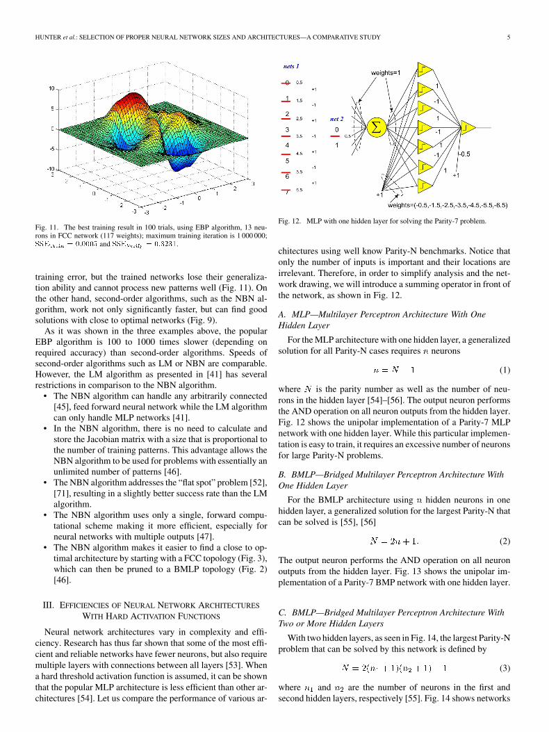
Fig. 11. The best training result in 100 trials, using EBP algorithm, 13 neu-rons in FCC network (117 weights); maximum training iteration is 1 000 000;�� and �� .

training error, but the trained networks lose their generaliza-tion ability and cannot process new patterns well (Fig. 11). Onthe other hand, second-order algorithms, such as the NBN al-gorithm, work not only significantly faster, but can find goodsolutions with close to optimal networks (Fig. 9).

As it was shown in the three examples above, the popularEBP algorithm is 100 to 1000 times slower (depending onrequired accuracy) than second-order algorithms. Speeds ofsecond-order algorithms such as LM or NBN are comparable.However, the LM algorithm as presented in [41] has severalrestrictions in comparison to the NBN algorithm.

• The NBN algorithm can handle any arbitrarily connected[45], feed forward neural network while the LM algorithmcan only handle MLP networks [41].

• In the NBN algorithm, there is no need to calculate andstore the Jacobian matrix with a size that is proportional tothe number of training patterns. This advantage allows theNBN algorithm to be used for problems with essentially anunlimited number of patterns [46].

• The NBN algorithm addresses the “flat spot” problem [52],[71], resulting in a slightly better success rate than the LMalgorithm.

• The NBN algorithm uses only a single, forward compu-tational scheme making it more efficient, especially forneural networks with multiple outputs [47].

• The NBN algorithm makes it easier to find a close to op-timal architecture by starting with a FCC topology (Fig. 3),which can then be pruned to a BMLP topology (Fig. 2)[46].

III. EFFICIENCIES OF NEURAL NETWORK ARCHITECTURES

WITH HARD ACTIVATION FUNCTIONS

Neural network architectures vary in complexity and effi-ciency. Research has thus far shown that some of the most effi-cient and reliable networks have fewer neurons, but also requiremultiple layers with connections between all layers [53]. Whena hard threshold activation function is assumed, it can be shownthat the popular MLP architecture is less efficient than other ar-chitectures [54]. Let us compare the performance of various ar-

Fig. 12. MLP with one hidden layer for solving the Parity-7 problem.

chitectures using well know Parity-N benchmarks. Notice thatonly the number of inputs is important and their locations areirrelevant. Therefore, in order to simplify analysis and the net-work drawing, we will introduce a summing operator in front ofthe network, as shown in Fig. 12.

A. MLP—Multilayer Perceptron Architecture With OneHidden Layer

For the MLP architecture with one hidden layer, a generalizedsolution for all Parity-N cases requires neurons

(1)

where is the parity number as well as the number of neu-rons in the hidden layer [54]–[56]. The output neuron performsthe AND operation on all neuron outputs from the hidden layer.Fig. 12 shows the unipolar implementation of a Parity-7 MLPnetwork with one hidden layer. While this particular implemen-tation is easy to train, it requires an excessive number of neuronsfor large Parity-N problems.

B. BMLP—Bridged Multilayer Perceptron Architecture WithOne Hidden Layer

For the BMLP architecture using hidden neurons in onehidden layer, a generalized solution for the largest Parity-N thatcan be solved is [55], [56]

(2)

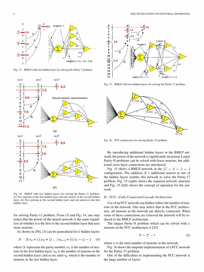
The output neuron performs the AND operation on all neuronoutputs from the hidden layer. Fig. 13 shows the unipolar im-plementation of a Parity-7 BMP network with one hidden layer.

C. BMLP—Bridged Multilayer Perceptron Architecture WithTwo or More Hidden Layers

With two hidden layers, as seen in Fig. 14, the largest Parity-Nproblem that can be solved by this network is defined by

(3)

where and are the number of neurons in the first andsecond hidden layers, respectively [55]. Fig. 14 shows networks


Fig. 13. BMLP with one hidden layer for solving the Parity-7 problem.

Fig. 14. BMLP with two hidden layers for solving the Parity-11 problem.(a) Two neurons in the first hidden layer and one neuron in the second hiddenlayer. (b) Two neurons in the second hidden layer and one neuron in the firsthidden layer.

for solving Parity-11 problem. From (3) and Fig. 14, one maynotice that the power of the neural network is the same regard-less of whether it is the first or the second hidden layer that usesmore neurons.

As shown in [56], (3) can be generalized for hidden layers

(4)

where represents the parity number; is the number of neu-rons in the first hidden layer; is the number of neurons in thesecond hidden layer; and so on; until which is the number ofneurons in the last hidden layer.

Fig. 15. BMLP with two hidden layers for solving the Parity-17 problem.

Fig. 16. FCC architecture for solving Parity-15 problem.

By introducing additional hidden layers in the BMLP net-work, the power of the network is significantly increased. LargerParity-N problems can be solved with fewer neurons, but addi-tional cross-layer connections are introduced.

Fig. 15 shows a BMLP network in theconfiguration. The addition of 1 additional neuron in one ofthe hidden layers enables this network to solve the Parity-17problem. Fig. 15 (right) shows the required network structureand Fig. 15 (left) shows the concept of operation for the net-work.

D. FCC—Fully Connected Cascade Architecture

Use of an FCC network can further reduce the number of neu-rons in the network. One may notice that in the FCC architec-ture, all neurons in the network are directly connected. Whensome of these connections are removed the network will be re-duced to the BMLP architecture.

The largest Parity-N problem which can be solved withneurons in the FCC architecture is [55]

(5)

where is the total number of neurons in the network.Fig. 16 shows the unipolar implementation of a FCC network

for the Parity-15 problem.One of the difficulties in implementing the FCC network is

the large number of layers.


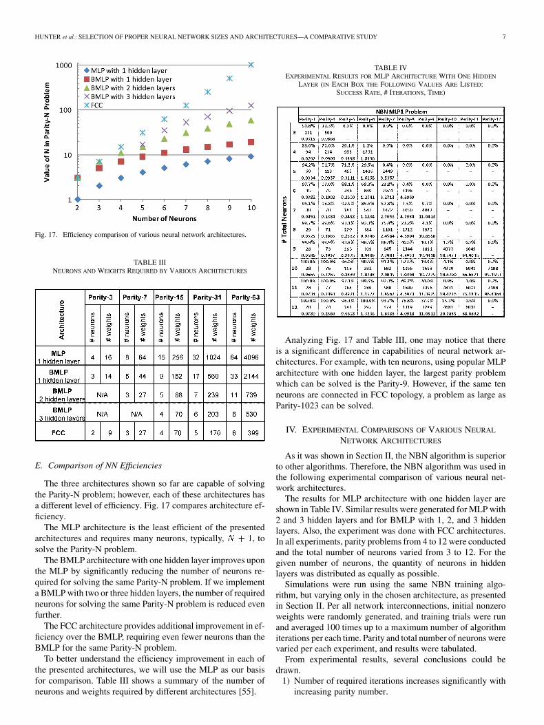
Fig. 17. Efficiency comparison of various neural network architectures.

TABLE IIINEURONS AND WEIGHTS REQUIRED BY VARIOUS ARCHITECTURES

E. Comparison of NN Efficiencies

The three architectures shown so far are capable of solvingthe Parity-N problem; however, each of these architectures hasa different level of efficiency. Fig. 17 compares architecture ef-ficiency.

The MLP architecture is the least efficient of the presentedarchitectures and requires many neurons, typically, , tosolve the Parity-N problem.

The BMLP architecture with one hidden layer improves uponthe MLP by significantly reducing the number of neurons re-quired for solving the same Parity-N problem. If we implementa BMLP with two or three hidden layers, the number of requiredneurons for solving the same Parity-N problem is reduced evenfurther.

The FCC architecture provides additional improvement in ef-ficiency over the BMLP, requiring even fewer neurons than theBMLP for the same Parity-N problem.

To better understand the efficiency improvement in each ofthe presented architectures, we will use the MLP as our basisfor comparison. Table III shows a summary of the number ofneurons and weights required by different architectures [55].

TABLE IVEXPERIMENTAL RESULTS FOR MLP ARCHITECTURE WITH ONE HIDDEN

LAYER (IN EACH BOX THE FOLLOWING VALUES ARE LISTED:SUCCESS RATE, # ITERATIONS, TIME)

Analyzing Fig. 17 and Table III, one may notice that thereis a significant difference in capabilities of neural network ar-chitectures. For example, with ten neurons, using popular MLParchitecture with one hidden layer, the largest parity problemwhich can be solved is the Parity-9. However, if the same tenneurons are connected in FCC topology, a problem as large asParity-1023 can be solved.

IV. EXPERIMENTAL COMPARISONS OF VARIOUS NEURAL

NETWORK ARCHITECTURES

As it was shown in Section II, the NBN algorithm is superiorto other algorithms. Therefore, the NBN algorithm was used inthe following experimental comparison of various neural net-work architectures.

The results for MLP architecture with one hidden layer areshown in Table IV. Similar results were generated for MLP with2 and 3 hidden layers and for BMLP with 1, 2, and 3 hiddenlayers. Also, the experiment was done with FCC architectures.In all experiments, parity problems from 4 to 12 were conductedand the total number of neurons varied from 3 to 12. For thegiven number of neurons, the quantity of neurons in hiddenlayers was distributed as equally as possible.

Simulations were run using the same NBN training algo-rithm, but varying only in the chosen architecture, as presentedin Section II. Per all network interconnections, initial nonzeroweights were randomly generated, and training trials were runand averaged 100 times up to a maximum number of algorithmiterations per each time. Parity and total number of neurons werevaried per each experiment, and results were tabulated.

From experimental results, several conclusions could bedrawn.

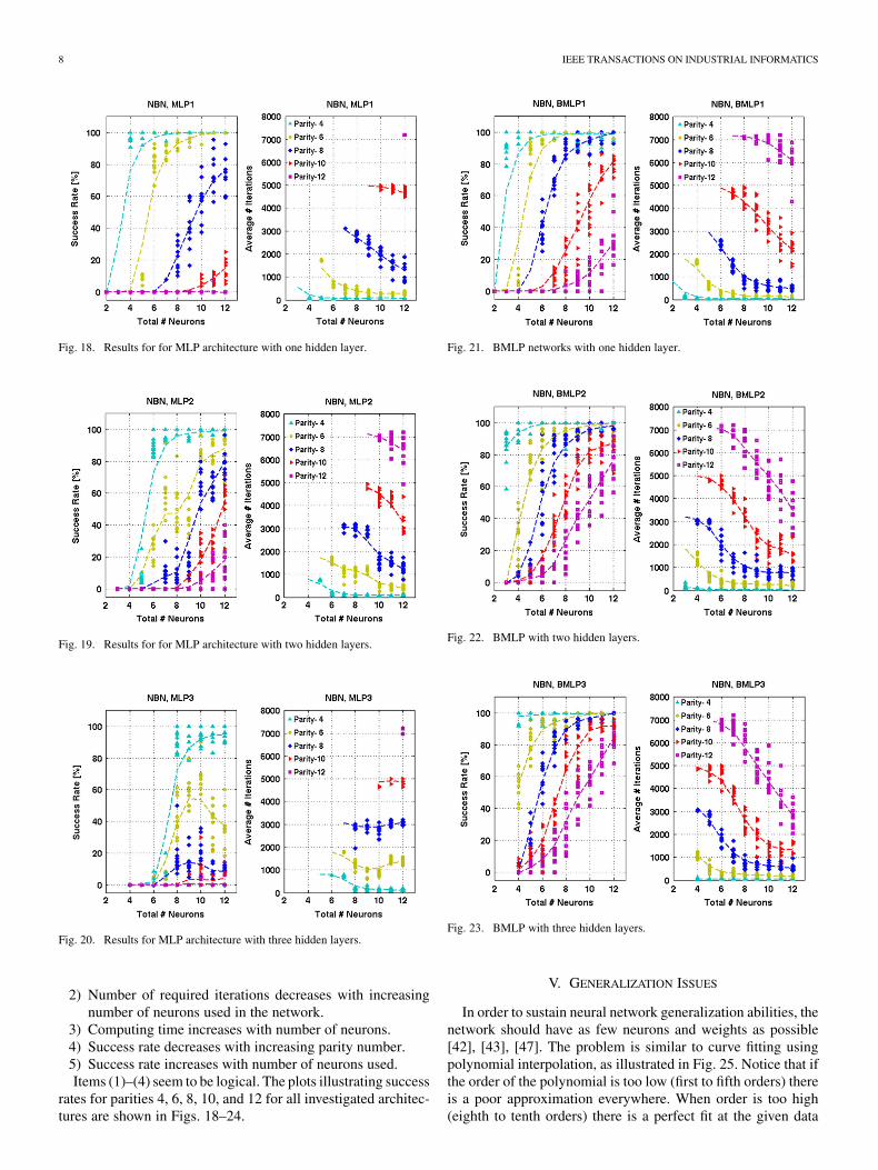
1) Number of required iterations increases significantly withincreasing parity number.


Fig. 18. Results for for MLP architecture with one hidden layer.

Fig. 19. Results for for MLP architecture with two hidden layers.

Fig. 20. Results for MLP architecture with three hidden layers.

2) Number of required iterations decreases with increasingnumber of neurons used in the network.

3) Computing time increases with number of neurons.4) Success rate decreases with increasing parity number.5) Success rate increases with number of neurons used.Items (1)–(4) seem to be logical. The plots illustrating success

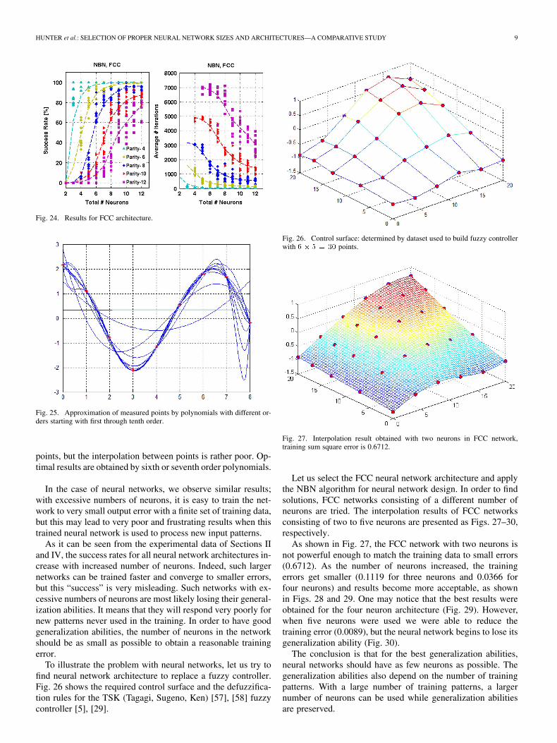
rates for parities 4, 6, 8, 10, and 12 for all investigated architec-tures are shown in Figs. 18–24.

Fig. 21. BMLP networks with one hidden layer.

Fig. 22. BMLP with two hidden layers.

Fig. 23. BMLP with three hidden layers.

V. GENERALIZATION ISSUES

In order to sustain neural network generalization abilities, thenetwork should have as few neurons and weights as possible[42], [43], [47]. The problem is similar to curve fitting usingpolynomial interpolation, as illustrated in Fig. 25. Notice that ifthe order of the polynomial is too low (first to fifth orders) thereis a poor approximation everywhere. When order is too high(eighth to tenth orders) there is a perfect fit at the given data


Fig. 24. Results for FCC architecture.

Fig. 25. Approximation of measured points by polynomials with different or-ders starting with first through tenth order.

points, but the interpolation between points is rather poor. Op-timal results are obtained by sixth or seventh order polynomials.

In the case of neural networks, we observe similar results;with excessive numbers of neurons, it is easy to train the net-work to very small output error with a finite set of training data,but this may lead to very poor and frustrating results when thistrained neural network is used to process new input patterns.

As it can be seen from the experimental data of Sections IIand IV, the success rates for all neural network architectures in-crease with increased number of neurons. Indeed, such largernetworks can be trained faster and converge to smaller errors,but this “success” is very misleading. Such networks with ex-cessive numbers of neurons are most likely losing their general-ization abilities. It means that they will respond very poorly fornew patterns never used in the training. In order to have goodgeneralization abilities, the number of neurons in the networkshould be as small as possible to obtain a reasonable trainingerror.

To illustrate the problem with neural networks, let us try tofind neural network architecture to replace a fuzzy controller.Fig. 26 shows the required control surface and the defuzzifica-tion rules for the TSK (Tagagi, Sugeno, Ken) [57], [58] fuzzycontroller [5], [29].

Fig. 26. Control surface: determined by dataset used to build fuzzy controllerwith � � � � �� points.

Fig. 27. Interpolation result obtained with two neurons in FCC network,training sum square error is 0.6712.

Let us select the FCC neural network architecture and applythe NBN algorithm for neural network design. In order to findsolutions, FCC networks consisting of a different number ofneurons are tried. The interpolation results of FCC networksconsisting of two to five neurons are presented as Figs. 27–30,respectively.

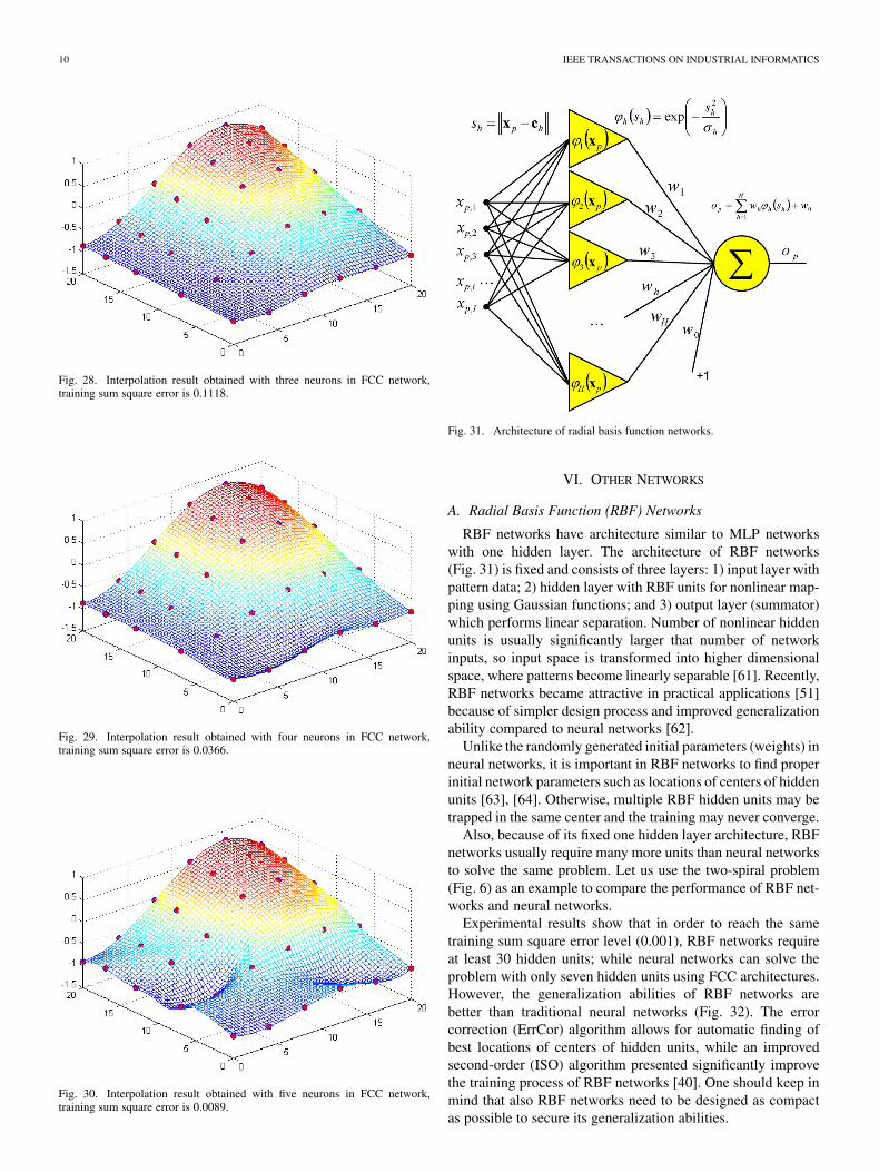
As shown in Fig. 27, the FCC network with two neurons isnot powerful enough to match the training data to small errors(0.6712). As the number of neurons increased, the trainingerrors get smaller (0.1119 for three neurons and 0.0366 forfour neurons) and results become more acceptable, as shownin Figs. 28 and 29. One may notice that the best results wereobtained for the four neuron architecture (Fig. 29). However,when five neurons were used we were able to reduce thetraining error (0.0089), but the neural network begins to lose itsgeneralization ability (Fig. 30).

The conclusion is that for the best generalization abilities,neural networks should have as few neurons as possible. Thegeneralization abilities also depend on the number of trainingpatterns. With a large number of training patterns, a largernumber of neurons can be used while generalization abilitiesare preserved.


Fig. 28. Interpolation result obtained with three neurons in FCC network,training sum square error is 0.1118.

Fig. 29. Interpolation result obtained with four neurons in FCC network,training sum square error is 0.0366.

Fig. 30. Interpolation result obtained with five neurons in FCC network,training sum square error is 0.0089.

Fig. 31. Architecture of radial basis function networks.

VI. OTHER NETWORKS

A. Radial Basis Function (RBF) Networks

RBF networks have architecture similar to MLP networkswith one hidden layer. The architecture of RBF networks(Fig. 31) is fixed and consists of three layers: 1) input layer withpattern data; 2) hidden layer with RBF units for nonlinear map-ping using Gaussian functions; and 3) output layer (summator)which performs linear separation. Number of nonlinear hiddenunits is usually significantly larger that number of networkinputs, so input space is transformed into higher dimensionalspace, where patterns become linearly separable [61]. Recently,RBF networks became attractive in practical applications [51]because of simpler design process and improved generalizationability compared to neural networks [62].

Unlike the randomly generated initial parameters (weights) inneural networks, it is important in RBF networks to find properinitial network parameters such as locations of centers of hiddenunits [63], [64]. Otherwise, multiple RBF hidden units may betrapped in the same center and the training may never converge.

Also, because of its fixed one hidden layer architecture, RBFnetworks usually require many more units than neural networksto solve the same problem. Let us use the two-spiral problem(Fig. 6) as an example to compare the performance of RBF net-works and neural networks.

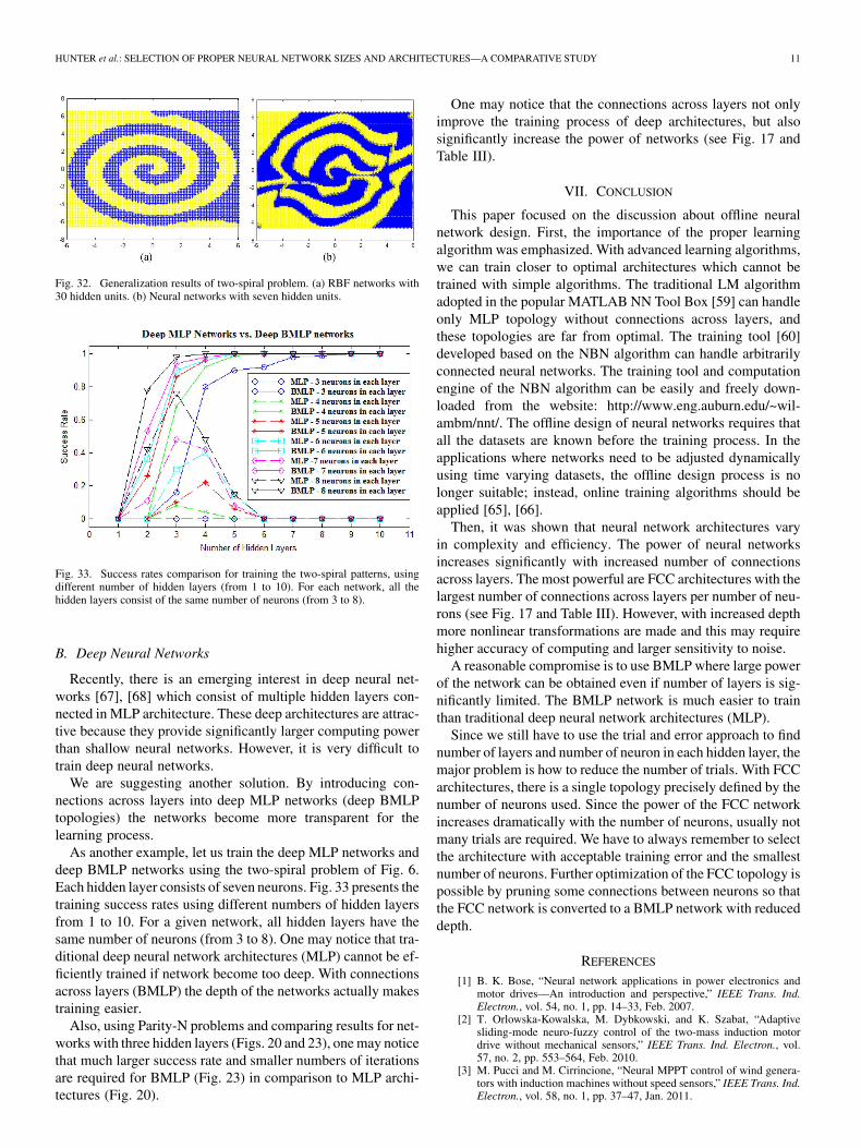
Experimental results show that in order to reach the sametraining sum square error level (0.001), RBF networks requireat least 30 hidden units; while neural networks can solve theproblem with only seven hidden units using FCC architectures.However, the generalization abilities of RBF networks arebetter than traditional neural networks (Fig. 32). The errorcorrection (ErrCor) algorithm allows for automatic finding ofbest locations of centers of hidden units, while an improvedsecond-order (ISO) algorithm presented significantly improvethe training process of RBF networks [40]. One should keep inmind that also RBF networks need to be designed as compactas possible to secure its generalization abilities.


Fig. 32. Generalization results of two-spiral problem. (a) RBF networks with30 hidden units. (b) Neural networks with seven hidden units.

Fig. 33. Success rates comparison for training the two-spiral patterns, usingdifferent number of hidden layers (from 1 to 10). For each network, all thehidden layers consist of the same number of neurons (from 3 to 8).

B. Deep Neural Networks

Recently, there is an emerging interest in deep neural net-works [67], [68] which consist of multiple hidden layers con-nected in MLP architecture. These deep architectures are attrac-tive because they provide significantly larger computing powerthan shallow neural networks. However, it is very difficult totrain deep neural networks.

We are suggesting another solution. By introducing con-nections across layers into deep MLP networks (deep BMLPtopologies) the networks become more transparent for thelearning process.

As another example, let us train the deep MLP networks anddeep BMLP networks using the two-spiral problem of Fig. 6.Each hidden layer consists of seven neurons. Fig. 33 presents thetraining success rates using different numbers of hidden layersfrom 1 to 10. For a given network, all hidden layers have thesame number of neurons (from 3 to 8). One may notice that tra-ditional deep neural network architectures (MLP) cannot be ef-ficiently trained if network become too deep. With connectionsacross layers (BMLP) the depth of the networks actually makestraining easier.

Also, using Parity-N problems and comparing results for net-works with three hidden layers (Figs. 20 and 23), one may noticethat much larger success rate and smaller numbers of iterationsare required for BMLP (Fig. 23) in comparison to MLP archi-tectures (Fig. 20).

One may notice that the connections across layers not onlyimprove the training process of deep architectures, but alsosignificantly increase the power of networks (see Fig. 17 andTable III).

VII. CONCLUSION

This paper focused on the discussion about offline neuralnetwork design. First, the importance of the proper learningalgorithm was emphasized. With advanced learning algorithms,we can train closer to optimal architectures which cannot betrained with simple algorithms. The traditional LM algorithmadopted in the popular MATLAB NN Tool Box [59] can handleonly MLP topology without connections across layers, andthese topologies are far from optimal. The training tool [60]developed based on the NBN algorithm can handle arbitrarilyconnected neural networks. The training tool and computationengine of the NBN algorithm can be easily and freely down-loaded from the website: http://www.eng.auburn.edu/~wil-ambm/nnt/. The offline design of neural networks requires thatall the datasets are known before the training process. In theapplications where networks need to be adjusted dynamicallyusing time varying datasets, the offline design process is nolonger suitable; instead, online training algorithms should beapplied [65], [66].

Then, it was shown that neural network architectures varyin complexity and efficiency. The power of neural networksincreases significantly with increased number of connectionsacross layers. The most powerful are FCC architectures with thelargest number of connections across layers per number of neu-rons (see Fig. 17 and Table III). However, with increased depthmore nonlinear transformations are made and this may requirehigher accuracy of computing and larger sensitivity to noise.

A reasonable compromise is to use BMLP where large powerof the network can be obtained even if number of layers is sig-nificantly limited. The BMLP network is much easier to trainthan traditional deep neural network architectures (MLP).

Since we still have to use the trial and error approach to findnumber of layers and number of neuron in each hidden layer, themajor problem is how to reduce the number of trials. With FCCarchitectures, there is a single topology precisely defined by thenumber of neurons used. Since the power of the FCC networkincreases dramatically with the number of neurons, usually notmany trials are required. We have to always remember to selectthe architecture with acceptable training error and the smallestnumber of neurons. Further optimization of the FCC topology ispossible by pruning some connections between neurons so thatthe FCC network is converted to a BMLP network with reduceddepth.

REFERENCES

[1] B. K. Bose, “Neural network applications in power electronics andmotor drives—An introduction and perspective,” IEEE Trans. Ind.Electron., vol. 54, no. 1, pp. 14–33, Feb. 2007.

[2] T. Orlowska-Kowalska, M. Dybkowski, and K. Szabat, “Adaptivesliding-mode neuro-fuzzy control of the two-mass induction motordrive without mechanical sensors,” IEEE Trans. Ind. Electron., vol.57, no. 2, pp. 553–564, Feb. 2010.

[3] M. Pucci and M. Cirrincione, “Neural MPPT control of wind genera-tors with induction machines without speed sensors,” IEEE Trans. Ind.Electron., vol. 58, no. 1, pp. 37–47, Jan. 2011.


[4] V. N. Ghate and S. V. Dudul, “Cascade neural-network-based faultclassifier for three-phase induction motor,” IEEE Trans. Ind. Electron.,vol. 58, no. 5, pp. 1555–1563, May 2011.

[5] C. Xia, C. Guo, and T. Shi, “A neural-network-identifier and fuzzy-controller-based algorithm for dynamic decoupling control of perma-nent-magnet spherical motor,” IEEE Trans. Ind. Electron., vol. 57, no.8, pp. 2868–2878, Aug. 2010.

[6] F. F. M. El-Sousy, “Hybri-based wavelet-neural-network trackingcontrol for permanent-magnet synchronous motor servo drives,” IEEETrans. Ind. Electron., vol. 57, no. 9, pp. 3157–3166, Sep. 2010.

[7] F. F. M. El-Sousy, “Hybrid �� based wavelet-neural-networktracking control for permanent-magnet synchronous motor servodrives,” IEEE Trans. Ind. Electron., vol. 57, no. 9, pp. 3157–3166,Sep. 2010.

[8] Q. N. Le and J. W. Jeon, “Neural-network-based low-speed-dampingcontroller for stepper motor with an FPGA,” IEEE Trans. Ind. Elec-tron., vol. 57, no. 9, pp. 3167–3180, Sep. 2010.

[9] C.-H. Lu, “Wavelet fuzzy neural networks for identification and pre-dictive control of dynamic systems,” IEEE Trans. Ind. Electron., vol.58, no. 7, pp. 3046–3058, Jul. 2011.

[10] R. H. Abiyev and O. Kaynak, “Type 2 fuzzy neural structure for identi-fication and control of time-varying plants,” IEEE Trans. Ind. Electron.,vol. 57, no. 12, pp. 4147–4159, Dec. 2010.

[11] M. A. S. K. Khan and M. A. Rahman, “Implementation of a wavelet-based MRPID controller for benchmark thermal system,” IEEE Trans.Ind. Electron., vol. 57, no. 12, pp. 4160–4169, Dec. 2010.

[12] A. Bhattacharya and C. Chakraborty, “A shunt active power filter withenhanced performance using ANN-based predictive and adaptive con-trollers,” IEEE Trans. Ind. Electron., vol. 58, no. 2, pp. 421–428, Feb.2011.

[13] J. Lin and R.-J. Lian, “Intelligent control of active suspension systems,”IEEE Trans. Ind. Electron., vol. 58, no. 2, pp. 618–628, Feb. 2011.

[14] Z. Lin, J. Wang, and D. Howe, “A learning feed-forward current con-troller for linear reciprocating vapor compressors,” IEEE Trans. Ind.Electron., vol. 58, no. 8, pp. 3383–3390, Aug. 2011.

[15] M. O. Efe, “Neural network assisted computationally simple PI Dcontrol of a quadrotor UAV,” IEEE Trans. Ind. Informat., vol. 7, no. 2,pp. 354–361, May 2011.

[16] T. Orlowska-Kowalska and M. Kaminski, “FPGA implementation ofthe multilayer neural network for the speed estimation of the two-massdrive system,” IEEE Trans. Ind. Informat., vol. 7, no. 3, pp. 436–445,Aug. 2011.

[17] C.-F. Juang, Y.-C. Chang, and C.-M. Hsiao, “Evolving gaits ofa hexapod robot by recurrent neural networks with symbioticspecies-based particle swarm optimization,” IEEE Trans. Ind. Elec-tron., vol. 58, no. 7, pp. 3110–3119, Jul. 2011.

[18] C.-C. Tsai, H.-C. Huang, and S.-C. Lin, “Adaptive neural network con-trol of a self-balancing two-wheeled scooter,” IEEE Trans. Ind. Elec-tron., vol. 57, no. 4, pp. 1420–1428, Apr. 2010.

[19] G. W. Chang, C.-I. Chen, and Y.-F. Teng, “Radial-basis-func-tion-based neural network for harmonic detection,” IEEE Trans. Ind.Electron., vol. 57, no. 6, pp. 2171–2179, Jun. 2010.

[20] R.-J. Wai and C.-Y. Lin, “Active low-frequency ripple control forclean-energy power-conditioning mechanism,” IEEE Trans. Ind.Electron., vol. 57, no. 11, pp. 3780–3792, Nov. 2010.

[21] Yahyaoui, N. Fnaiech, and F. Fnaiech, “A suitable initialization proce-dure for speeding a neural network job-shop scheduling,” IEEE Trans.Ind. Electron., vol. 58, no. 3, pp. 1052–1060, Mar. 2011.

[22] V. Machado, A. Neto, and J. D. de Melo, “A neural network multiagentarchitecture applied to industrial networks for dynamic allocation ofcontrol strategies using standard function blocks,” IEEE Trans. Ind.Electron., vol. 57, no. 5, pp. 1823–1834, May 2010.

[23] M. Charkhgard and M. Farrokhi, “State-of-charge estimation forlithium-ion batteries using neural networks and EKF,” IEEE Trans.Ind. Electron., vol. 57, no. 12, Dec. 2010.

[24] M. Wilamowski and O. Kaynak, “Oil well diagnosis by sensing ter-minal characteristics of the induction motor,” IEEE Trans. Ind. Elec-tron., vol. 47, no. 5, pp. 1100–1107, Oct. 2000.

[25] N. J. Cotton and B. M. Wilamowski, “Compensation of nonlinearitiesusing neural networks implemented on inexpensive microcontrollers,”IEEE Trans. Ind. Electron., vol. 58, no. 3, pp. 733–740, Mar. 2011.

[26] A. Gomperts, A. Ukil, and F. Zurfluh, “Development and implemen-tation of parameterized FPGA-based general purpose neural networksfor online applications,” IEEE Trans. Ind. Informat., vol. 7, no. 1, pp.78–89, Feb. 2011.

[27] E. Monmasson, L. Idkhajine, M. N. Cirstea, I. Bahri, A. Tisan, and M.W. Naouar, “FPGAs in industrial control applications,” IEEE Trans.Ind. Informat., vol. 7, no. 2, pp. 224–243, May 2011.

[28] A. Dinu, M. N. Cirstea, and S. E. Cirstea, “Direct neural-network hard-ware-implementation algorithm,” IEEE Trans. Ind. Electron., vol. 57,no. 5, pp. 1845–1848, May 2010.

[29] A. Malinowski and H. Yu, “Comparison of various embedded systemtechnologies for industrial applications,” IEEE Trans. Ind. Informat.,vol. 7, no. 2, pp. 244–254, May 2011.

[30] D. E. Rumelhart, G. E. Hinton, and R. J. Williams, “Learning repre-sentations by back-propagating errors,” Nature, vol. 323, pp. 533–536,1986.

[31] P. J. Werbos, “Back-propagation: Past and future,” in Proc. Int. Conf.Neural Netw., San Diego, CA, 1988, pp. 343–354, 1.

[32] S. Ferrari and M. Jensenius, “A constrained optimization approach topreserving prior knowledge during incremental training,” IEEE Trans.Neural Netw., vol. 19, no. 6, pp. 996–1009, Jun. 2008.

[33] Q. Song, J. C. Spall, Y. C. Soh, and J. Ni, “Robust neural networktracking controller using simultaneous perturbation stochastic approx-imation,” IEEE Trans. Neural Netw., vol. 19, no. 5, pp. 817–835, May2008.

[34] A. Slowik, “Application of an adaptive differential evolution algorithmwith multiple trial vectors to artificial neural network training,” IEEETrans. Ind. Electron., vol. 58, no. 8, pp. 3160–3167, Aug. 2011.

[35] V. V. Phansalkar and P. S. Sastry, “Analysis of the back-propagationalgorithm with momentum,” IEEE Trans. Neural Netw., vol. 5, no. 3,pp. 505–506, Mar. 1994.

[36] A. Salvetti and B. M. Wilamowski, “Introducing stochastic processeswithin the backpropagation algorithm for improved convergence,” inProc. Artif. Neural Netw. Eng.–ANNIE’94.

[37] B. M. Wilamowski and L. Torvik, “Modification of gradient com-putation in the back-propagation algorithm,” in Artif. Neural Netw.Eng.–ANNIE’93.

[38] M. Riedmiller and H. Braun, “A direct adaptive method for fasterbackpropagation learning: The RPROP algorithm,” in Proc. Int. Conf.Neural Netw., San Francisco, CA, 1993, pp. 586–591.

[39] S. E. Fahlman, An Empirical Study of Learning Speed in Backpropa-gation Networks 1988.

[40] K. Levenberg, “A method for the solution of certain problems in leastsquares,” Quart. Appl. Mach., vol. 5, pp. 164–168, 1944.

[41] M. T. Hagan and M. B. Menhaj, “Training feedforward networks withthe Marquardt algorithm,” IEEE Trans. Neural Netw., vol. 5, no. 6, pp.989–993, Nov. 1994.

[42] B. M. Wilamowski, “Neural network architectures and learning algo-rithms,” IEEE Ind. Electron. Mag., vol. 3, no. 4, pp. 56–63, Dec. 2009.

[43] B. M. Wilamowski, “Challenges in applications of computational in-telligence in industrial electronics,” in Proc. Int. Symp. Ind. Electron.-ISIE’10, Bari, Italy, Jul. 4–7, 2010, pp. 15–22.

[44] N. J. Cotton, B. M. Wilamowski, and G. Dundar, “A neural networkimplementation on an inexpensive eight bit microcontroller,” in Proc.12th Int. Conf. Intell. Eng. Syst.–INES’08, Miami, Florida, USA, Feb.25–29, 2008, pp. 109–114.

[45] B. M. Wilamowski, N. J. Cotton, O. Kaynak, and G. Dundar, “Com-puting gradient vector and jacobian matrix in arbitrarily connectedneural networks,” IEEE Trans. Ind. Electron., vol. 55, no. 10, pp.3784–3790, Oct. 2008.

[46] B. M. Wilamowski and H. Yu, “Improved computation for LevenbergMarquardt training,” IEEE Trans. Neural Netw., vol. 21, no. 6, pp.930–937, Jun. 2010.

[47] B. M. Wilamowski and H. Yu, “Neural network learning without back-propgation,” IEEE Trans. Neural Netw., vol. 21, no. 11, pp. 1793–1803,Nov. 2010.

[48] J. R. Alvarez-Sanchez, “Injecting knowledge into the solution of thetwo-spiral problem,” Neural Comput. Appl., vol. 8, pp. 265–272, Aug.1999.

[49] S. Wan and L. E. Banta, “Parameter incremental learning algorithmfor neural networks,” IEEE Trans. Neural Netw., vol. 17, no. 6, pp.1424–1438, Jun. 200.

[50] S. E. Fahlman and C. Lebiere, , D. S. Touretzky, Ed., “The cascade-correction learning architecture,” in Advances in Neural InformationProcessing Systems 2. San Mateo, CA: Morgan Kaufmann.

[51] H. Yu, T. T. Xie, S. Paszczynski, and B. M. Wilamowski, “Advantagesof radial basis function networks for dynamic system design,” IEEETrans. Ind. Electron., vol. 58, no. 12, pp. 5438–5450, Dec. 2011.

[52] B. M. Wilamowski and L. Torvik, “Modification of gradient computa-tion in the back-propagation algorithm,” in Proc. Artif. Neural Netw.Eng.–ANNIE’93, St. Louis, MO, Nov. 14–17, 1993, pp. 175–180.

[53] B. M. Wilamowski, D. Hunter, and A. Malinowski, “Solving parity-nproblems with feedforward neural network,” in Proc. Int. JointConf. Neural Netw.–IJCNN’03, Portland, OR, Jul. 20–23, 2003, pp.2546–2551.


[54] S. Trenn, “Multilayer perceptrions: Approximation order and neces-sary number of hidden units,” IEEE Trans. Neural Netw., vol. 19, no.5, pp. 836–844, May 2008.

[55] D. Hunter and B. M. Wilamowski, “Parallel multi-layer neural net-work architecture with improved efficiency,” in Proc. 4th Conf. HumanSyst. Interactions–HSI’11, Yokohama, Japan, May 19–21, 2011, pp.299–304.

[56] B. M. Wilamowski, H. Yu, and K. Chung, “Parity-N problems as avehicle to compare efficiency of neural network architectures,” in In-dustrial Electronics Handbook, 2nd ed. Boca Raton, FL: CRC Press,2011, vol. 5, Intelligent Systems, ch. 10, pp. 10-1–10-8.

[57] T. Sugeno and G. T. Kang, “Structure identification of fuzzy model,”Fuzzy Sets and Systems, vol. 28, no. 1, pp. 15–33, 1988.

[58] T. T. Xie, H. Yu, and B. M. Wilamowski, “Replacing fuzzy systemswith neural networks,” in Proc. IEEE Human Syst. Interaction Conf.–HSI’10, Rzeszow, Poland, May 13–15, 2010, pp. 189–193.

[59] H. B. Demuth and M. Beale, Neural Network Toolbox: For Use WithMATLAB. Natick, MA: Mathworks, 2000.

[60] H. Yu and B. M. Wilamowski, “Efficient and reliable training of neuralnetworks,” in Proc. IEEE Human Syst. Interaction Conf.–HSI’09,Catania, Italy, May 21–23, 2009, pp. 109–115.

[61] T. M. Cover, “Geometrical and statistical properties of systems oflinear inequalities with applications in pattern recognition,” IEEETrans. Electron. Comput., vol. EC-14, pp. 326–334.

[62] T. T. Xie, H. Yu, and B. M. Wilamowski, “Comparison of traditionalneural networks and radial basis function networks,” in Proc. 20thIEEE Int. Symp. Ind. Electron.–ISIE’11, Gdansk, Poland, Jun. 27–30,2011, pp. 1194–1199.

[63] S. Chen, C. F. N. Cowan, and P. M. Grant, “Orthogonal least squareslearning algorithm for radial basis function networks,” IEEE Trans.Neural Netw., vol. 2, no. 2, pp. 302–309, Mar. 1991.

[64] G. B. Huang, P. Saratchandran, and N. Sundararajan, “A generalizedgrowing and pruning RBF (GGAP-RBF) neural network for functionapproximation,” IEEE Trans. Neural Netw., vol. 16, no. 1, pp. 57–67,Jan. 2005.

[65] M. Pucci and M. Cirrincione, “Neural MPPT control of wind genera-tors with induction machines without speed sensors,” IEEE Trans. Ind.Electron., vol. 58, no. 1, pp. 37–47, Jan. 2011.

[66] Q. N. Le and J. W. Jeon, “Neural-network-based low-speed-dampingcontroller for stepper motor with an FPGA,” IEEE Trans. Ind. Elec-tron., vol. 57, no. 9, pp. 3167–3180, Sep. 2010.

[67] K. Chen and A. Salman, “Learning speaker-specific characteristicswith a deep neural architecture,” IEEE Trans. Neural Netw., vol. 22,no. 11, pp. 1744–1756, 2011.

[68] I. Arel, D. C. Rose, and T. P. Karnowski, “Deep machine learning—Anew frontier in artificial intelligence research,” IEEE Comput. Intell.Mag., vol. 5, no. 4, pp. 13–18, 2010.

[69] Intelligent Engineering Systems Through Artificial Neural Networks.New York: ASME, 1994, vol. 4, pp. 205–209.

[70] Intelligent Engineering Systems Through Artificial Neural Networks.New York: ASME, 1993, vol. 3, pp. 175–180, Also in.

[71] Intelligent Engineering Systems Through Artificial Neural Networks.New York: ASME, 1993, vol. 3, pp. 175–180.

David Hunter currently is in the Ph.D. program atAuburn University focusing on development of newneural network architectures and training methods.He received his M.S. in computer engineering in2003 from the University of Idaho. Previously, Mr.Hunter worked for 15 years in the semiconductorindustry with a focus in photolithography, metrology,and defects.

Hao Yu (S’10) received the Ph.D. degree in electricaland computer engineering from Auburn University,Auburn, AL, in 2011.

He was a Research Assistant with the Departmentof Electrical and Computer Engineering, AuburnUniversity. He is currently working in Lattice Semi-conductor. His research interests include machinelearning, FPGA development, and EDA.

Dr. Yu serves as Reviewer for the IEEETRANSACTIONS ON INDUSTRIAL ELECTRONICS, theIEEE TRANSACTIONS ON INDUSTRIAL INFORMATICS,

and the IEEE TRANSACTIONS ON NEURAL NETWORKS.

Michael S. Pukish III (S’07) is currently workingtowards the Ph.D. degree at Auburn University,Auburn, AL, studying neural network architecturesand training methods and applied problems.

He has developed testing suites comprised oforiginal PCB and FPGA designs for complexsystem-in-chip RFICs. Previously, he worked as aPCB Designer and analytical tools and applicationdeveloper for various aerospace, radio astronomyand auditory technology companies and researchgroups.

Janusz Kolbusz received the M.Sc. degree in infor-matics and automatics engineering from the RzeszowUniversity of Technology, Rzeszow, Poland, in 1998,and the Ph.D. degree in telecommunications from theUniversity of Technology and Life Sciences, Byd-goszcz, Poland, in 2010.

Since 1998, he has been working at Informa-tion Technology and Management, Rzeszow. Hisresearch interests focus on operations systems,computer networks, architectural systems devel-opment, quality of service and survivability of the

next-generation optical transport networks.

Bogdan M. Wilamowski (SM’83–F’00) receivedthe M.S. degree in computer engineering in 1966,the Ph.D. degree in neural computing in 1970, andthe Dr.Habil. degree in integrated circuit design in1977, all from Gdansk University of Technology,Gdansk, Poland.

He was with the Gdansk University of Tech-nology; the University of Information Technologyand Management, Rzeszow, Poland; Auburn Uni-versity, Auburn, AL; University of Arizona, Tucson;University of Wyoming, Laramie; and the University

of Idaho, Moscow. He is currently the Director of the Alabama Micro/NanoScience and Technology Center, Auburn University.

Dr. Wilamowski was the Vice President of the IEEE Computational Intelli-gence Society (2000–2004) and the President of the IEEE Industrial ElectronicsSociety (2004–2005). He served as an Associate Editor in numerous journals.He was the Editor-in-Chief of the IEEE TRANSACTIONS ON INDUSTRIAL

ELECTRONICS from 2007 to 2010

ieee transactions on industrial informatics …wilambm/pap/2012/tii-pukish-2187914-x.pdf · ieee...

Documents