ieee transactions on image processing, …projectmagma.net/~melekor/tmp/image interpolation...

IEEE TRANSACTIONS ON IMAGE PROCESSING, VOL. 17, NO. 6, JUNE 2008 887

Image Interpolation by Adaptive 2-D AutoregressiveModeling and Soft-Decision Estimation

Xiangjun Zhang and Xiaolin Wu, Senior Member, IEEE

Abstract—The challenge of image interpolation is to preservespatial details. We propose a soft-decision interpolation techniquethat estimates missing pixels in groups rather than one at a time.The new technique learns and adapts to varying scene structuresusing a 2-D piecewise autoregressive model. The model parame-ters are estimated in a moving window in the input low-resolutionimage. The pixel structure dictated by the learnt model is enforcedby the soft-decision estimation process onto a block of pixels, in-cluding both observed and estimated. The result is equivalent tothat of a high-order adaptive nonseparable 2-D interpolation filter.This new image interpolation approach preserves spatial coher-ence of interpolated images better than the existing methods, and itproduces the best results so far over a wide range of scenes in bothPSNR measure and subjective visual quality. Edges and texturesare well preserved, and common interpolation artifacts (blurring,ringing, jaggies, zippering, etc.) are greatly reduced.

Index Terms—Autoregressive process, image interpolation,image modeling, optimization, soft decision estimation.

I. INTRODUCTION

ONE of the most important quality metrics of digital im-ages is spatial resolution. Despite steady increase of native

sensor resolutions of digital cameras and scanners, new appli-cations will always emerge that demand even higher spatial res-olution. Image interpolation is an algorithmic means to increasethe native resolution of an input image. An obvious applicationof image interpolation is the reproduction of images capturedby digital cameras for high quality prints in magazines, cata-logs, wall posters, or even home use. Another important appli-cation is upconversion of standard-definition video frames forplayback on high-definition television receivers and computermonitors. Besides consumer electronics, image interpolation isbeneficial and in some cases even necessary in computer vision,surveillance, medical imaging, remote sensing, and other fields.

Many image interpolation techniques of different tradeoffsbetween computational complexity and reproduction qualitywere developed. Popular methods, as commonly used inimage/video software and hardware products, are bilinearinterpolation, cubic convolution interpolation [1] and cubic

Manuscript received September 1, 2007; revised March 13, 2008. This workwas supported by the Natural Sciences and Engineering Research Council ofCanada. This paper was presented in part at the 2007 IEEE International Con-ference on Image Processing. The associate editor coordinating the review ofthis manuscript and approving it for publication was Prof. Vicent Caselles.

The authors are with the Department of Electrical and ComputerEngineering McMaster University Hamilton, Ontario, ON L8S 4K1Canada (e-mail: [email protected]; [email protected];[email protected]).

Digital Object Identifier 10.1109/TIP.2008.924279

spline interpolation [2]. The main advantage of these methodsis their relatively low complexity. Their common drawbackis the inability to adapt to varying pixel structures in a scene,due to the use of scene-independent interpolators. As a result,they are all susceptible to defects such as jaggies, blurring, andringing.

With ever-increasing computation power in image and videoprocessing, more sophisticated adaptive image interpolationmethods were proposed in recent years. Many researchers ad-vocated the approach of edge-guided interpolation. Jensen andAnastassiou published a scheme that detects edges and fits themwith some templates to improve the visual perception of inter-polated images [3]. Carrato and Tenze used some predeterminededge patterns to optimize the parameters in the interpolationoperator [4]. To preserve edge structures in interpolation, Li andOrchard proposed to estimate the covariance of high-resolution(HR) image from the covariance of the low-resolution (LR)image, and then interpolate the missing pixels based on theestimated covariance [5]. This edge-directed interpolation workwas cast by Muresan and Parks into the framework of adaptiveoptimal recovery [6]. Alternatively, Zhang and Wu proposedto interpolate a missing pixel in multiple directions, and thenfuse the directional interpolation results by minimum meansquare-error estimation [7].

Wavelets were also used in image interpolation. The idea isto exploit the statistical similarity between different scales of awavelet-decomposed image. The interpolation is done by pre-dicting the HR details from the LR observation [8]–[10]. Wuand Zhang studied image interpolation in a framework of pat-tern classification [11]. In [12], Malgouyres and Guichard an-alyzed some linear and nonlinear image enlargement methodstheoretically and experimentally.

The reproduction quality of any image interpolation algo-rithm primarily depends on its adaptability to varying pixelstructures across an image. In fact, modeling of nonstationarityof image signals is a common challenge facing many imageprocessing tasks, such as compression, restoration, denoising,and enhancement. We had a measured success in this regardin a research on predictive lossless image compression [13].In that work, a natural image is modeled as a piecewise 2-Dautoregressive process. The model parameters are estimated onthe fly for each pixel using sample statistics of a local window,assuming that the image is piecewise stationary. In this paper,we extend this approach to image interpolation. An obviousdifference is in that the sample set for parameter estimation hasto be causal to the current pixel for predictive coding, but doesnot need to be so for interpolation, which is to the advantageof the latter task. On the other hand, for image interpolation

1057-7149/$25.00 © 2008 IEEE

888 IEEE TRANSACTIONS ON IMAGE PROCESSING, VOL. 17, NO. 6, JUNE 2008

the fit of the model to the true HR image signal is made moredifficult by the fact that only a LR version of the original canbe observed.

All image interpolation methods involve fitting missing pixelsto some sample structure learnt from the LR image. This is bestaccomplished by estimating a block of missing pixels in relationto the nearby known pixels rather than estimating the individualmissing pixels in isolation as done up to now. The main con-tribution of this paper is a new image interpolation technique,called soft-decision adaptive interpolation (SAI). The SAI tech-nique, via a natural integration of piecewise 2-D autoregressivemodeling and block estimation, achieves superior image inter-polation results to those reported in the literature. It is shownthat the new SAI technique is equivalent to interpolation usingan adaptive nonseparable 2-D filter of high order.

The rest of the paper is structured as follows. Section II de-fines a 2-D piecewise autoregressive (PAR) image model to fa-cilitate the subsequent development. Section III presents themost important result of this paper: a soft-decision estimationtechnique for adaptive image interpolation (SAI). Section IVdiscusses how to estimate the PAR model parameters in the LRimage. Implementation details of the SAI algorithm are pre-sented in Section V, where the reader can also gain an insightinto the inner work of the SAI technique. Experimental resultsand a comparison study with some existing popular image in-terpolation techniques are presented in Section VI. Section VIIconcludes.

II. PIECEWISE STATIONARY AUTOREGRESSIVE MODEL

For the purpose of adaptive image interpolation, we modelthe image as a piecewise autoregressive (PAR) process

(1)

where is a spatial template for the regression operation. Theterm is a random perturbation independent of spatial loca-tion and the image signal, and it accounts for both fractal-like fine details of image signal and measurement noise. The va-lidity of the PAR model hinges on a mechanism that adjusts themodel parameters to local pixel structures. The fact thatsemantically meaningful image constructs, such as edges andsurface textures, are formed by spatially coherent contiguouspixels, suggests piecewise statistical stationarity of the imagesignal. In other words, in the setting of the PAR model, the pa-rameters remain constant or near constant in a smalllocality, although they may and often do vary significantly indifferent segments of a scene. The piecewise stationarity makesit possible to learn pixel structures such as edges and texturesby fitting samples of a local window to the PAR model.

The validity of the PAR model with locally adaptive param-eters is corroborated by the success of this modeling techniquein lossless image compression. Among all known lossless imagecoding methods, including CALIC [14], TMW [15], and invert-ible integer wavelets [16], those that employ the PAR modelwith adjusted parameters on a pixel-by-pixel basis have deliv-ered the lowest lossless bit rates [13], [17]. In the principle ofKolmogorov complexity, the true model of a stochastic process

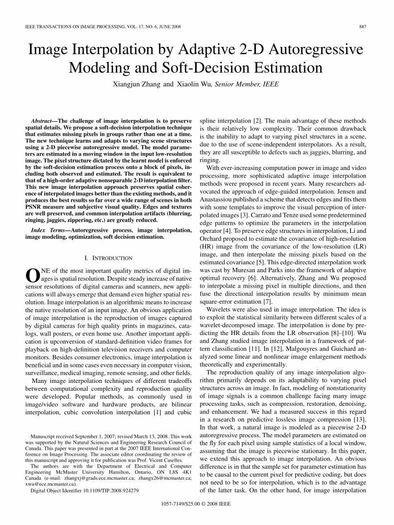
Fig. 1. Formation of a LR image from a HR image by down-sampling. Thesolid dots are the LR image pixels and the circles are the missing HR pixels.Interpolation is done in two passes. The first pass interpolates the missingpixels marked by shaded circles, and the second pass interpolates the remainingmissing pixels marked by empty circles.

is the one that yields the minimum description length. Thus, wehave strong empirical evidence to support the appropriatenessand usefulness of the PAR model for natural images.

In Section III, we will integrate the PAR model into a soft-de-cision estimation framework for the purpose of image interpo-lation, and develop the SAI algorithm.

III. ADAPTIVE INTERPOLATION WITH SOFT DECISION

First we introduce some notations that are necessary for thedescription of the SAI algorithm. Let be the HR image tobe estimated by interpolating the LR image observed. TheLR image is a down sampled version of the HR imageby a factor of two as illustrated by Fig. 1. Let and

be the pixels of images and , respectively. Wewrite the neighbors of pixel location in the HR image as ,

. Since implies , we also write anHR pixel as (likewise, as ) when it is in theLR image, , as well.

The SAI algorithm interpolates the missing pixels in intwo passes in a coarse to fine progression. The work of the twopasses is shown by Fig. 1, in which the solid dots are knownLR pixels, the shaded dots are those missing pixels to be inter-polated in the first pass, and the empty dots are the remainingmissing pixels to be interpolated in the second pass. The pixelsgenerated by the first pass and the known LR pixels form a quin-cunx sublattice of the HR image (the union of solid and shadeddots). The second pass completes the reconstruction of the HRimage by interpolating the other quincunx sublattice of emptydots.

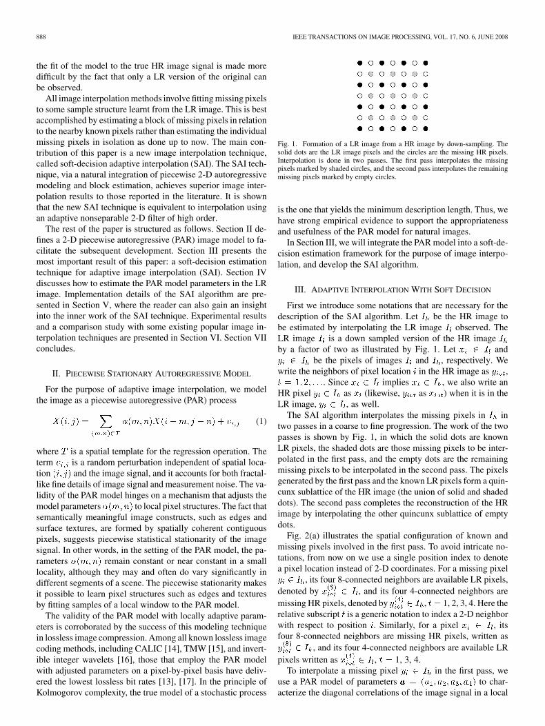
Fig. 2(a) illustrates the spatial configuration of known andmissing pixels involved in the first pass. To avoid intricate no-tations, from now on we use a single position index to denotea pixel location instead of 2-D coordinates. For a missing pixel

, its four 8-connected neighbors are available LR pixels,denoted by , and its four 4-connected neighbors aremissing HR pixels, denoted by , 1, 2, 3, 4. Here therelative subscript is a generic notation to index a 2-D neighborwith respect to position . Similarly, for a pixel , itsfour 8-connected neighbors are missing HR pixels, written as

, and its four 4-connected neighbors are available LRpixels written as , 1, 3, 4.

To interpolate a missing pixel in the first pass, weuse a PAR model of parameters to char-acterize the diagonal correlations of the image signal in a local

ZHANG AND WU: IMAGE INTERPOLATION BY ADAPTIVE 2-D AUTOREGRESSIVE MODELING AND SOFT-DECISION ESTIMATION 889

Fig. 2. (a) Spatial configuration in the first pass. (b) PAR model parameters�� and �� in relationship to spatial correlationsof pixels.

window [see Fig. 2(b)]. Using the simplified notations to re-place , we rewrite (1) as

(2)

With the PAR model, we interpolate missing pixelsin window by a least-squares block

estimation

(3)

The above image interpolation approach has an importantdistinction from its predecessors (e.g., [2] and [5]). Existingimage interpolation methods estimate each missing pixel inde-pendently from others, which we characterize as hard-decisionestimation. In contrast, we adopt a strategy of soft-decisionestimation in resemblance to block decoding of error correctioncodes. Rather than estimating one sample at a time in isolation,the objective function of (3) requires all missing pixels in a localwindow to be estimated jointly. Moreover, the soft-decision

estimation approach brings in a new feedback mechanism thatis the second term in (3). This additional term requires theestimates of the missing HR pixels to fit the known LRpixels with the very same PAR model that fitsto . Aided by the feedback mechanism that accounts formutual influences between the estimates of the missing pixelsin a local window , the SAI algorithm can mitigate errors ofhard-decision estimation by preventing the PAR model, whenapplied to estimated HR pixels , from being violated onneighboring known LR pixels .

To include horizontal and vertical correlations into the SAI al-gorithm, we introduce four more parameterswhose geometric meanings are shown in Fig. 2(b). These pa-rameters are used to impose the same directional correlationbetween LR pixels and on between HR pixels and

, namely

(4)

The soft-decision estimation technique can incorporate (4) into(3). However, one should practice caution since the pixelsand in (4) are all unknown. By using a Lagrangian multi-plier to regulate the contribution of (4), we extend (3) to thefollowing constrained optimal block estimation problem [see(5), shown at the bottom of the page]. In minimizing , the

value of is chosen such that

. The SAI algorithm iterates onuntil the constraint is satisfactorily met, by decreasing if theleft side of the constraint is less than the right side and vise versa.This constraint holds if the sample statistics is shift invariant inthe window . We observe that the value of is in the rangeof when meeting the constraint. For most natural im-ages, one can simply choose with no material loss ofperformance compared with the iteratively computed .

Compared to existing autoregressive methods that use param-eters only [5], [7], the SAI algorithm expands the model pa-rameter space by using two sets of parameters and . Theexpanded PAR model has the potential of representing the HRimage more accurately than in [5], [7]. However, to circumventthe risk of data overfitting, we do not directly use an autoregres-sive model of order 8, but rather split model parameters and

in two separate terms of the objective function (5). In fact, inseparation from , the parameters can be better estimated thanparameters using samples in the LR image, as we will see inSection IV.

subject to (5)


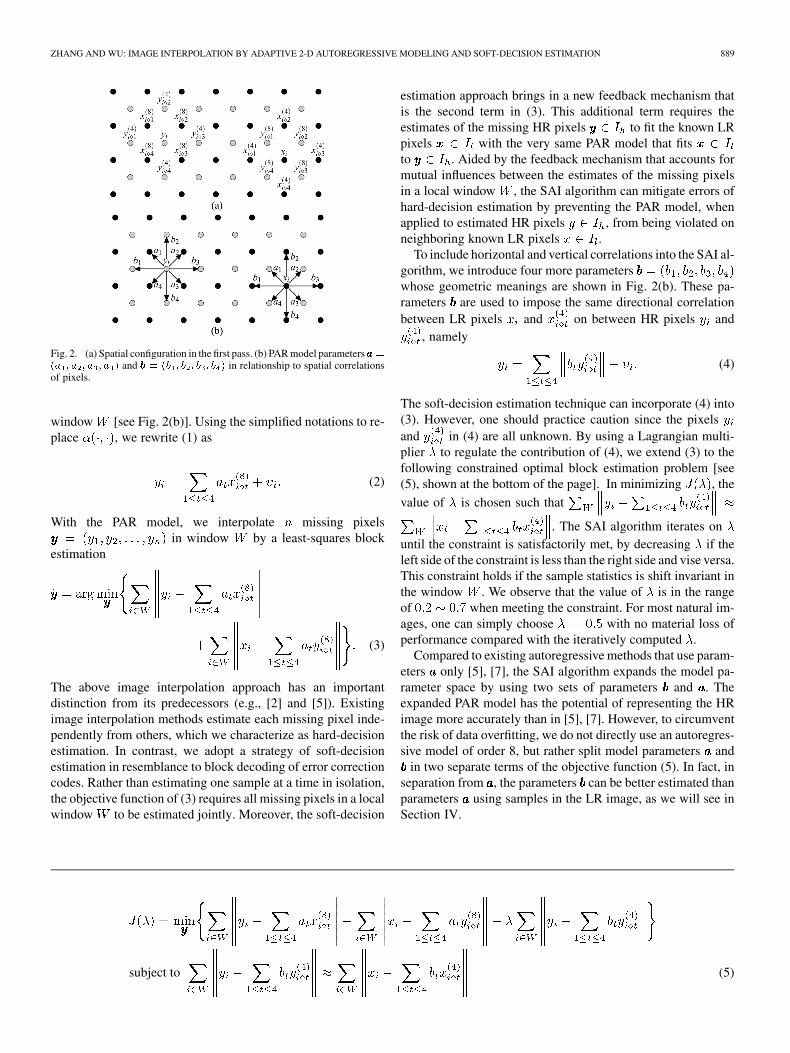
Fig. 3. Spatial configuration in the second pass of interpolation.

With the block-based soft-decision estimation and the in-creased order in piecewise autoregressive modeling, the newSAI algorithm achieves unprecedented interpolation accuracy.More importantly, it performs consistently well over a widerange of images, and the performance is far less sensitiveto feature scales than existing techniques. We will return tothese points in Section VI when the experimental results arepresented and discussed.

Up to now, we have only described the interpolation processof the first pass. Once the missing HR pixels in the first passare interpolated as described above, half of the HR pixels areobtained. The remaining half of the missing HR pixels are tobe interpolated in the second pass. The interpolation problemin the second pass is essentially the same as in the first pass.The only difference is that the SAI algorithm now interpolatesthe missing HR pixels using their four 4-connectedneighbors, which are either known in or estimated in the firstpass. The problem has the same formulation as in (5), if wesimply rotate the spatial configuration of Fig. 2(a) by 45 (seeFig. 3).

IV. MODEL PARAMETER ESTIMATION

A key to the success of the SAI algorithm is how well themodel parameters and in (5) can be estimated using LRimage samples. Referring to the spatial relation between thesamples in Fig. 4(b), one gets a linear least-square estimator ofthe model parameter vector

(6)

where are the four 4-connected neighbors of the locationin as labeled in Fig. 4(b). Note that the estimates of in (6)are made using the LR pixels that have the same spatialorientation and the same scale as the way the HR pixelsare related by in (5) [this is also clear in Fig. 2(b)]. Hence, theresulting estimates are optimal in the least-square sense underthe assumption that the sample covariances do not change in thelocal window , which is generally true for natural images.

However, the estimation of the model parameters is moreproblematic. One can simply, as proposed by Li and Orchard[5], compute via the following linear least-square estimation

(7)

Fig. 4. Sample relations in estimating model parameters. (a) Parameter ��,(b) parameter ��.

Fig. 5. Possible configuration used in the soft-decision interpolation algorithm.

where are the four 8-connected neighbors of the locationin as labeled in Fig. 4(a). The accuracy of (7) relies on a

stronger assumption that the correlation between pixels is un-changed in different scales. This is because the distance between

and in (7) is twice the distance between and in(5).

As argued in [5], the above assumption holds if the windowin question has edge(s) of a fixed orientation and of suffi-ciently large scale. However, experiments show (see results inSection VI) that previous edge-based interpolation methodsare prone to artifacts on small-scale spatial features of highcurvature, for which the second order statistics may differ fromLR to HR images. In such cases, the soft-decision estimationstrategy of (5) can moderate the effects of estimation errorsof (7), making the proposed SAI approach considerably morerobust.

V. ALGORITHM DETAILS

To perform soft-decision estimation, the SAI algorithm needsto operate on blocks of pixels. The neighboring blocks shouldhave some overlaps to prevent possible block visual artifacts.Many spatial configurations of the overlapped blocks can beused. To be concrete let us consider a particular configurationas illustrated in Fig. 5. As shown in the figure, a block of 12 un-known pixels , arranged in an octagonal window(bounded by the solid line in Fig. 5), are jointly estimated, con-strained by the 21 available LR pixels . Solvingthe least-squares problem of (5) in the octagonal window willyield a group of 12 estimated missing pixels. However, the SAI


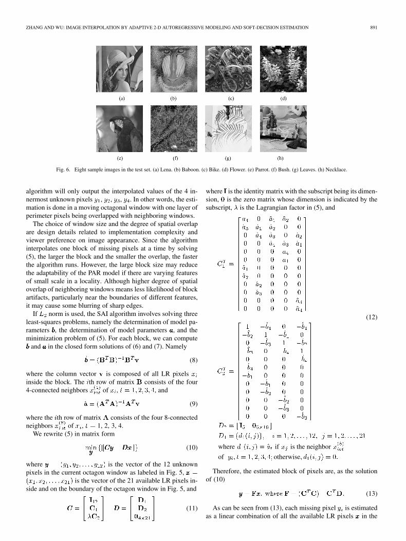
Fig. 6. Eight sample images in the test set. (a) Lena. (b) Baboon. (c) Bike. (d) Flower. (e) Parrot. (f) Bush. (g) Leaves. (h) Necklace.

algorithm will only output the interpolated values of the 4 in-nermost unknown pixels , , , . In other words, the esti-mation is done in a moving octagonal window with one layer ofperimeter pixels being overlapped with neighboring windows.

The choice of window size and the degree of spatial overlapare design details related to implementation complexity andviewer preference on image appearance. Since the algorithminterpolates one block of missing pixels at a time by solving(5), the larger the block and the smaller the overlap, the fasterthe algorithm runs. However, the large block size may reducethe adaptability of the PAR model if there are varying featuresof small scale in a locality. Although higher degree of spatialoverlap of neighboring windows means less likelihood of blockartifacts, particularly near the boundaries of different features,it may cause some blurring of sharp edges.

If norm is used, the SAI algorithm involves solving threeleast-squares problems, namely the determination of model pa-rameters , the determination of model parameters , and theminimization problem of (5). For each block, we can compute

and in the closed form solutions of (6) and (7). Namely

(8)

where the column vector is composed of all LR pixelsinside the block. The th row of matrix consists of the four4-connected neighbors of , , and

(9)

where the th row of matrix consists of the four 8-connectedneighbors of , 1, 2, 3, 4.

We rewrite (5) in matrix form

(10)

where is the vector of the 12 unknownpixels in the current octagon window as labeled in Fig. 5,

is the vector of the 21 available LR pixels in-side and on the boundary of the octagon window in Fig. 5, and

(11)

where is the identity matrix with the subscript being its dimen-sion, is the zero matrix whose dimension is indicated by thesubscript, is the Lagrangian factor in (5), and

(12)

where if is the neighbor

of otherwise

Therefore, the estimated block of pixels are, as the solutionof (10)

(13)

As can be seen from (13), each missing pixel is estimatedas a linear combination of all the available LR pixels in the


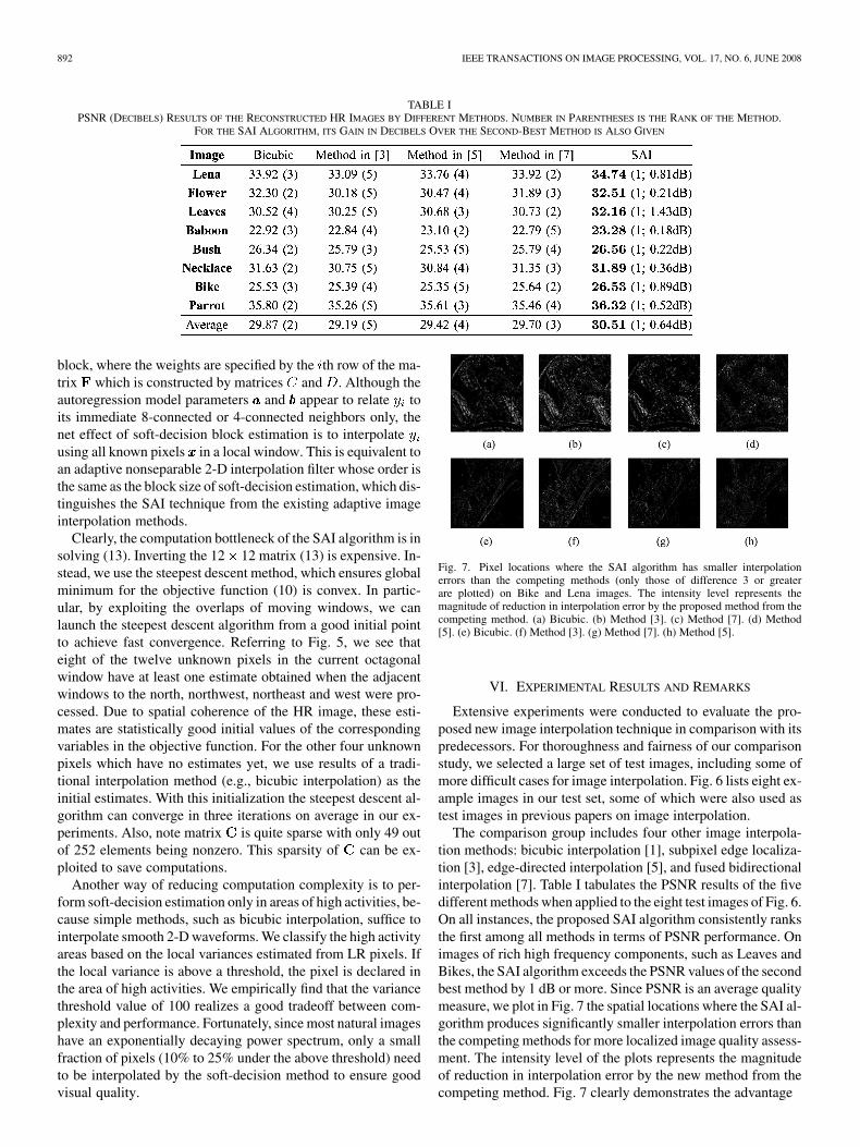
TABLE IPSNR (DECIBELS) RESULTS OF THE RECONSTRUCTED HR IMAGES BY DIFFERENT METHODS. NUMBER IN PARENTHESES IS THE RANK OF THE METHOD.

FOR THE SAI ALGORITHM, ITS GAIN IN DECIBELS OVER THE SECOND-BEST METHOD IS ALSO GIVEN

block, where the weights are specified by the th row of the ma-trix which is constructed by matrices and . Although theautoregression model parameters and appear to relate toits immediate 8-connected or 4-connected neighbors only, thenet effect of soft-decision block estimation is to interpolateusing all known pixels in a local window. This is equivalent toan adaptive nonseparable 2-D interpolation filter whose order isthe same as the block size of soft-decision estimation, which dis-tinguishes the SAI technique from the existing adaptive imageinterpolation methods.

Clearly, the computation bottleneck of the SAI algorithm is insolving (13). Inverting the 12 12 matrix (13) is expensive. In-stead, we use the steepest descent method, which ensures globalminimum for the objective function (10) is convex. In partic-ular, by exploiting the overlaps of moving windows, we canlaunch the steepest descent algorithm from a good initial pointto achieve fast convergence. Referring to Fig. 5, we see thateight of the twelve unknown pixels in the current octagonalwindow have at least one estimate obtained when the adjacentwindows to the north, northwest, northeast and west were pro-cessed. Due to spatial coherence of the HR image, these esti-mates are statistically good initial values of the correspondingvariables in the objective function. For the other four unknownpixels which have no estimates yet, we use results of a tradi-tional interpolation method (e.g., bicubic interpolation) as theinitial estimates. With this initialization the steepest descent al-gorithm can converge in three iterations on average in our ex-periments. Also, note matrix is quite sparse with only 49 outof 252 elements being nonzero. This sparsity of can be ex-ploited to save computations.

Another way of reducing computation complexity is to per-form soft-decision estimation only in areas of high activities, be-cause simple methods, such as bicubic interpolation, suffice tointerpolate smooth 2-D waveforms. We classify the high activityareas based on the local variances estimated from LR pixels. Ifthe local variance is above a threshold, the pixel is declared inthe area of high activities. We empirically find that the variancethreshold value of 100 realizes a good tradeoff between com-plexity and performance. Fortunately, since most natural imageshave an exponentially decaying power spectrum, only a smallfraction of pixels (10% to 25% under the above threshold) needto be interpolated by the soft-decision method to ensure goodvisual quality.

Fig. 7. Pixel locations where the SAI algorithm has smaller interpolationerrors than the competing methods (only those of difference 3 or greaterare plotted) on Bike and Lena images. The intensity level represents themagnitude of reduction in interpolation error by the proposed method from thecompeting method. (a) Bicubic. (b) Method [3]. (c) Method [7]. (d) Method[5]. (e) Bicubic. (f) Method [3]. (g) Method [7]. (h) Method [5].

VI. EXPERIMENTAL RESULTS AND REMARKS

Extensive experiments were conducted to evaluate the pro-posed new image interpolation technique in comparison with itspredecessors. For thoroughness and fairness of our comparisonstudy, we selected a large set of test images, including some ofmore difficult cases for image interpolation. Fig. 6 lists eight ex-ample images in our test set, some of which were also used astest images in previous papers on image interpolation.

The comparison group includes four other image interpola-tion methods: bicubic interpolation [1], subpixel edge localiza-tion [3], edge-directed interpolation [5], and fused bidirectionalinterpolation [7]. Table I tabulates the PSNR results of the fivedifferent methods when applied to the eight test images of Fig. 6.On all instances, the proposed SAI algorithm consistently ranksthe first among all methods in terms of PSNR performance. Onimages of rich high frequency components, such as Leaves andBikes, the SAI algorithm exceeds the PSNR values of the secondbest method by 1 dB or more. Since PSNR is an average qualitymeasure, we plot in Fig. 7 the spatial locations where the SAI al-gorithm produces significantly smaller interpolation errors thanthe competing methods for more localized image quality assess-ment. The intensity level of the plots represents the magnitudeof reduction in interpolation error by the new method from thecompeting method. Fig. 7 clearly demonstrates the advantage


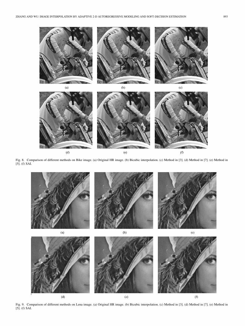
Fig. 8. Comparison of different methods on Bike image. (a) Original HR image. (b) Bicubic interpolation. (c) Method in [3]. (d) Method in [7]. (e) Method in[5]. (f) SAI.

Fig. 9. Comparison of different methods on Lena image. (a) Original HR image. (b) Bicubic interpolation. (c) Method in [3]. (d) Method in [7]. (e) Method in[5]. (f) SAI.


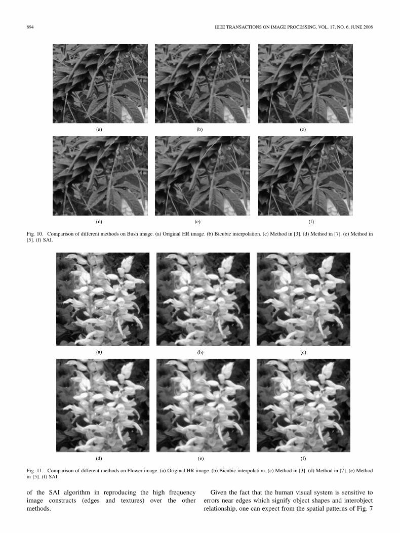
Fig. 10. Comparison of different methods on Bush image. (a) Original HR image. (b) Bicubic interpolation. (c) Method in [3]. (d) Method in [7]. (e) Method in[5]. (f) SAI.

Fig. 11. Comparison of different methods on Flower image. (a) Original HR image. (b) Bicubic interpolation. (c) Method in [3]. (d) Method in [7]. (e) Methodin [5]. (f) SAI.

of the SAI algorithm in reproducing the high frequencyimage constructs (edges and textures) over the othermethods.

Given the fact that the human visual system is sensitive toerrors near edges which signify object shapes and interobjectrelationship, one can expect from the spatial patterns of Fig. 7


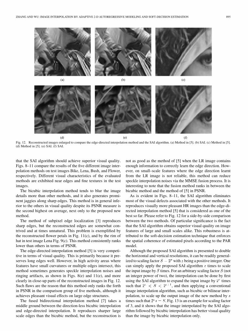
Fig. 12. Reconstructed images enlarged to compare the edge-directed interpolation method and the SAI algorithm. (a) Method in [5]. (b) SAI. (c) Method in [5].(d) Method in [5]. (e) SAI. (f) SAI.

that the SAI algorithm should achieve superior visual quality.Figs. 8–11 compare the results of the five different image inter-polation methods on test images Bike, Lena, Bush, and Flower,respectively. Different visual characteristics of the evaluatedmethods are exhibited near edges and fine textures in the testimages.

The bicubic interpolation method tends to blur the imagedetails more than other methods, and it also generates promi-nent jaggies along sharp edges. This method is in general infe-rior to the others in visual quality despite its PSNR measure isthe second highest on average, next only to the proposed newmethod.

The method of subpixel edge localization [3] reproducessharp edges, but the reconstructed edges are somewhat con-trived and at times unnatural. This problem is exemplified bythe reconstructed flower petals in Fig. 11(c), and by the rim ofhat in test image Lena Fig. 9(c). This method consistently rankslower than others in terms of PSNR.

The edge-directed interpolation method [5] is very competi-tive in terms of visual quality. This is primarily because it pre-serves long edges well. However, in high activity areas wherefeatures have small curvatures or multiple edges intersect, thismethod sometimes generates speckle interpolation noises andringing artifacts, as shown in Figs. 8(e) and 11(e), and moreclearly in close-up parts of the reconstructed images in Fig. 12.Such flaws are the reason that this method only ranks the forthin PSNR in the comparison group of five methods, although itachieves pleasant visual effects on large edge structures.

The fused bidirectional interpolation method [7] takes amiddle ground between the direction-less bicubic interpolationand edge-directed interpolation. It reproduces sharper largescale edges than the bicubic method, but the reconstruction is

not as good as the method of [5] when the LR image containsenough information to correctly learn the edge direction. How-ever, on small–scale features where the edge direction learntfrom the LR image is not reliable, this method can reducespeckle interpolation noises via the MMSE fusion process. It isinteresting to note that the fusion method ranks in between thebicubic method and the method of [5] in PSNR.

As is evident in Figs. 8–11, the SAI algorithm eliminatesmost of the visual defects associated with the other methods. Itreproduces visually more pleasant HR images than the edge-di-rected interpolation method [5] that is considered as one of thebest so far. Please refer to Fig. 12 for a side-by-side comparisonbetween the two methods. Of particular significance is the factthat the SAI algorithm obtains superior visual quality on imagefeatures of large and small scales alike. This robustness is at-tributed to the soft-decision estimation technique that enforcesthe spatial coherence of estimated pixels according to the PARmodel.

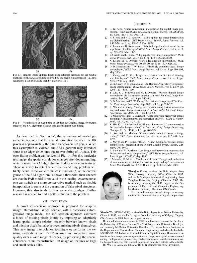
Although the proposed SAI algorithm is presented to doublethe horizontal and vertical resolutions, it can be readily general-ized to scaling factor with being a positive integer. Onecan simply apply the proposed SAI algorithm times to scalethe input image by times. For an arbitrary scaling factor (notan integer power of two), the interpolation can be done by firstusing the SAI algorithm to expand the input image by timessuch that , and then applying a conventionalimage interpolation algorithm, such as bicubic or bilinear inter-polation, to scale up the output image of the new method bytimes such that . Fig. 13 is an example for scaling factorof 3, and it shows that the image interpolated by the SAI algo-rithm followed by bicubic interpolation has better visual qualitythan the image by bicubic interpolation only.


Fig. 13. Images scaled up three times using different methods: (a) the bicubicmethod; (b) the SAI algorithm followed by the bicubic interpolation (i.e., firstscaling by a factor of 2 and then by a factor of 1.5).

Fig. 14. Visual effects of over-fitting of LR data. (a) Original image. (b) Outputimage of the SAI algorithm without safe guard against over-fitting.

As described in Section IV, the estimation of model pa-rameters assumes that the spatial correlation between the HRpixels is approximately the same as between LR pixels. Whenthis assumption is violated, the SAI algorithm may introducesome false edges or textures due to over-fitting of LR data. Thisover-fitting problem can be seen in Fig. 14. For this particulartest image, the spatial correlation changes after down sampling,which causes the SAI algorithm to produce erroneous textures.There is a way to detect where the over-fitting problem willlikely occur. If the value of the cost function (5) at the conver-gence of the SAI algorithm is above a threshold, then chancesare that the PAR model is not valid in the locality. As a recourse,one can switch to a more conservative method such as bicubicinterpolation to prevent the generation of false pixel structures.However, this also tends to blur some sharp edges. Furtherresearch is needed to find a better solution to the problem.

VII. CONCLUSION

A novel soft-decision approach is proposed for adaptiveimage interpolation. When coupled with a piecewise autore-gressive image model, the soft-decision approach estimatesa block of missing pixels jointly by imposing an adaptivelylearnt spatial sample relation not only between known pixelsand missing pixels but also between missing pixels themselves.This new image interpolation technique outperforms the ex-isting methods in both PSNR measure and subjective visualquality over a wide range of scenes, by preserving the spacialcoherence of the reconstructed HR image on features of largeand small scales alike.

REFERENCES

[1] R. G. Keys, “Cubic convolution interpolation for digital image pro-cessing,” IEEE TranS. Acoust., Speech, Signal Process., vol. ASSP-29,no. 6, pp. 1153–1160, Dec. 1981.

[2] H. S. Hou and H. C. Andrews, “Cubic splines for image interpolationand digital filtering,” IEEE Trans. Acoust., Speech, Signal Process., vol.ASSP-26, no. 6, pp. 508–517, Dec. 1978.

[3] K. Jensen and D. Anastassiou, “Subpixel edge localization and the in-terpolation of still images,” IEEE Trans. Image Process., vol. 4, no. 3,pp. 285–295, Mar. 1995.

[4] S. Carrato and L. Tenze, “A high quality 2� image interpolator,” IEEESignal Process. Lett., vol. 7, no. 6, pp. 132–135, Jun. 2000.

[5] X. Li and M. T. Orchard, “New edge-directed interpolation,” IEEETrans. Image Process., vol. 10, no. 10, pp. 1521–1527, Oct. 2001.

[6] D. D. Muresan and T. W. Parks, “Adaptively quadratic (aqua) imageinterpolation,” IEEE Trans. Image Process., vol. 13, no. 5, pp. 690–698,May 2004.

[7] L. Zhang and X. Wu, “Image interpolation via directional filteringand data fusion,” IEEE Trans. Image Process., vol. 15, no. 8, pp.2226–2238, Aug. 2006.

[8] W. K. Carey, D. B. Chuang, and S. S. Hemami, “Regularity-preservingimage interpolation,” IEEE Trans. Image Process., vol. 8, no. 9, pp.1293–1297, Sep. 1999.

[9] Y. Zhu, S. C. Schwartz, and M. T. Orchard, “Wavelet domain imageinterpolation via statistical estimation,” in Proc. Int. Conf. Image Pro-cessing, Sep. 2001, vol. 3, pp. 840–843.

[10] D. D. Muresan and T. W. Parks, “Prediction of image detail,” in Proc.Int. Conf. Image Processing, Sep. 2000, vol. 2, pp. 323–326.

[11] X. Wu and X. Zhang, “Image interpolation using texture orientationmap and kernel fisher discriminant,” in Proc. IEEE Int. Conf. ImageProcessing, Sep. 2005, vol. 1, pp. I–49–52.

[12] F. Malgouyres and F. Guichard, “Edge direction preserving imagezooming: A mathematical and numerical analysis,” SIAM J. Numer.Anal., vol. 39, pp. 1–37, 2001.

[13] X. Wu, K. U. Barthel, and W. Zhang, “Piecewise 2-D autoregressionfor predictive image coding,” in Proc. Int. Conf. Image Processing,Chicago, IL, Oct. 1998, vol. 3, pp. 901–904.

[14] X. Wu and N. Memon, “Context-based adaptive lossless imagecoding,” IEEE Trans. Commun., vol. 45, no. 4, pp. 437–444, Apr.1997.

[15] B. Meyer and P. Tischer, “TMW—A new method for lossless imagecompression,” presented at the Picture Coding Symp., Berlin, Ger-many, Oct. 1997.

[16] A. Said and W. Pearlman, “An image multiresolution representationfor lossless and lossy compression,” IEEE Trans. Image Process., vol.5, no. 9, pp. 1303–1330, Sep. 1996.

[17] I. Matsuda, H. Mori, J. Maeda, and S. Itoh, “Design and evaluationof minimum-rate predictors for lossless image coding,” (in Japanese)Trans. IEICE (DII), vol. J85-D-II, no. 3, pp. 448–456, Mar. 2002.

Xiangjun Zhang received the B.Sc. degree fromXi’an Jiaotong University, Xi’an, China, in 1997,and the M.S. degree in electrical engineering fromTsinghua University, Beijing, China, in 2002. Sheis currently pursuing the Ph.D. degree at the De-partment of Electrical and Computer Engineering,McMaster University, Hamilton, ON, Canada.

Her research interests include image processing,multimedia communication, and signal compression.

Xiaolin Wu (M’88–SM’96) received the B.Sc. degree from Wuhan University,China, in 1982, and the Ph.D. degree from the University of Calgary, Calgary,ON, Canada, in 1988, both in computer science.

He started his academic career in 1988, and has since been on the faculty atthe University of Western Ontario, New York Polytechnic University, Brooklyn,and currently McMaster University, Hamilton, ON, where he is a Professor inthe Department of Electrical and Computer Engineering, and where he holds theNSERC-DALSA Industrial Research Chair in Digital Cinema. His research in-terests include image processing, multimedia compression, joint source-channelcoding, multiple description coding, and network-aware visual communication.He has published over 180 research papers and holds two patents in these fields.

Dr. Wu is an Associate Editor of IEEE TRANSACTIONS ON MULTIMEDIA.

ieee transactions on image processing, …projectmagma.net/~melekor/tmp/image interpolation...

Documents