identifying politically connected … politically connected firms: a machine learning approach deni...
TRANSCRIPT

IDENTIFYING POLITICALLY
CONNECTED FIRMS: A MACHINE LEARNING
APPROACH
DENI MAZREKAJ, FRITZ SCHILTZ, VITEZSLAV TITL
KU LEUVEN, BELGIUM
Key words: Political Connections, Machine Learning, Random Forest, Boosting
Abstract
This article introduces machine learning techniques to identify politically connected firms. We use a
unique dataset of all contracting firms from the Czech Republic. In this dataset, various forms of
political connections can be determined from publicly available sources. The results indicate that
over 75% of firms with political connections can be accurately identified. The model obtains this high
accuracy by using only firm-level financial and industry indicators that are widely available in most
countries. Compared to the logistic regression model that is commonly used to predict binary
outcome variables, the proposed technique can increase the accuracy of predictions by up to 36%
using the same set of variables and the same data.

The opinions expressed and arguments employed herein are solely those of the authors and do not necessarily reflect the official views of the OECD or of its member countries. This document and any map included herein are without prejudice to the status of or sovereignty over any territory, to the delimitation of international frontiers and boundaries and to the name of any territory, city or area. This paper was submitted as part of a competitive call for papers on integrity and anti-corruption in the context of the 2019 OECD Global Anti-Corruption & Integrity Forum.

1
1. Introduction
Politically connected firms1 may generate substantial economic and welfare costs for the society. These
costs include higher product prices, poorly executed public works, and erosion in employment standards
(Fisman, Schulz, & Vikrant, 2014; Fisman & Wang, 2015). Moreover, political connections may have
macro-level implications on government efficiency as they induce misallocation of public funds (Cingano
& Pinotti, 2013; Goldman, Rocholl, & So, 2013; Titl & Geys, 2019). As a result, political connections
may impede economic growth (Olson, Sarna, & Swamy, 2000). Despite these negative implications of
political connections, both firms and politicians have an incentive to become politically connected
(Faccio, 2006; Sukhtankar, 2012). Firms may benefit from politically channelled loans and contracts,
regulatory benefits and soft budget constraints (Faccio, 2006). Likewise, politicians themselves also
benefit from firm connections as firms may garner votes and extract resources for political campaigns
(Sukhtankar, 2012).
Tackling the negative implications of political connections has proven to be difficult. For instance, one
way of establishing political connections may be through corporate donations. Therefore, many
developed countries such as France, Portugal, Poland, Canada, and the United States2 have introduced
a ban on corporate donations to political parties. However, one of the consequences of such a ban
could be lower transparency as firms that would have donated to political parties in the absence of a
ban may opt to establish political connections differently. They can obtain the connections by having
their top officers (CEO, president, chairperson) affiliated with politicians or by politicians having equity
in the firm (Faccio, 2006). These political connections are often even more difficult to track than
corporate donations. Nonetheless, for transparency and accountability as well as correct assessment
of welfare implications, it is critical to identify which firms are politically connected.
In this article, we introduce machine learning (ML) to predict which firms are politically connected. We
propose two methods that are implemented by iteratively constructing regression trees. These methods
add flexibility by capturing nonlinearities and complex interactions (Breiman, 2001). Recently, machine
learning has been used to improve predictions in many applications. Schiltz et al. (2018) use Monte
Carlo simulations to show how school rankings can be improved by machine learning predictions
relative to conventional regressions. Blumenstock (2016) and Jean et al. (2016) use satellite data to
identify areas with high poverty rates. Similarly, Antweiler & Frank (2004) predict stock prices using text
data from financial message boards. Ward (2017) illustrates that, compared to existing prediction
models, financial crises could have been more accurately predicted using classification trees and
ensembles – the same models used in this paper. Chalfin et al. (2016) provide examples on how these
same tools can be used to promote teachers or predict personnel productivity. Kleinberg et al. (2017)
show how machine predictions outperform human judgement with respect to jail-or-release decisions.
Thus, it is clear that machine learning has been used in many recent applications to predict various
outcomes. This recent surge in ML applications across several fields is driven by the ability of these
1 Political connections can be defined broadly as any link between politicians and private-sector firms. This includes personal ties, board memberships, ownership stakes and donations (Blau, 2017; Faccio, 2006; Fisman & Wang, 2015). 2 Regardless, U.S. companies may donate through so-called political action committees (PACs).

2
methods to improve predictions, as they allow for more effective ways to model complex relationships
(Mullainathan & Spiess, 2017; Varian, 2014).
We illustrate the added value of machine learning models in political science applications using a unique
dataset of all Czech contracting firms. The Czech Republic is a particularly interesting country to study,
as various forms of political connections can be determined from publicly available sources. We find
that over 75% of firms with political connections can be identified with publicly available financial and
industry indicators such as capital, financial and operational profits, or number of employees. Compared
to the logistic regression model used to predict binary outcome variables, the proposed technique can
increase the prediction accuracy by up to 36%.
The remainder of this article is structured as follows. Section II explains the machine learning technique
called extreme gradient boosting. In Section III, we construct the sample and define political connections
as well as variables used for prediction. Section IV shows how our proposed technique predicts political
connections with a much higher accuracy than the logistic regression model. Section V discusses how
public institutions and Nongovernmental Organizations (NGOs) can apply the proposed technique.
2. Methodology
As illustrated in the introduction, machine learning (ML) models are increasingly gaining popularity,
especially for prediction purposes (Mullainathan & Spiess, 2017). The motivation behind this surge is
that ML models more naturally accommodate discontinuous and nonlinear interactions (e.g. Varian,
2014). This is particularly useful for the prediction of political connections from firm characteristics as
we are able to capture complex patterns in firm and industry data.
We apply three different models to predict whether a firm is politically connected. We start from a logistic
regression, which is widely used to predict binary outcomes. Then, we improve the accuracy of
predictions using the same set of variables and the same data by introducing two classification tree
ensemble methods.3 The main advantage of tree-based methods is that interactions or nonlinearities
(e.g. higher degree polynomials) do not need to be modelled explicitly. The classification tree algorithm
considers all possible splits of all variables and chooses the one the maximizes the reduction in the
sum of squared residuals (SSR). The most predictive split (which reduces SSR the most) is placed on
the top of the tree. Repeating this process from top to bottom results in the construction of a
classification tree. This way, both continuous and categorical variables can be accommodated
simultaneously, while interactions and nonlinearities are included in the algorithm by construction.
To illustrate the flexibility of classification trees, consider a fictitious example in which we classify 100
firms as being politically connected or non-connected using only three variables: the number of
employees, the operational result, and registered capital. The tree displayed in Figure 1 depicts a
potential set of rules learned by the algorithm when classifying the 100 firms. Once this tree is
constructed, it suffices to follow the learned rule to obtain the predicted outcome of a new observation.
For example, a relatively large firm (more than 10,000 employees), with a strong operational result
3 See Online Appendix A for a technical description of both methodologies.

3
(more than 150 million euros), and less than 1 billion euros in registered capital has a higher probability
to be non-connected (8/15). Therefore, this firm will be classified as “non-connected”.
The accuracy of predictions can be improved considerably when combining information from several
classification trees into ensemble methods such as “random forest” or “boosting” (Breiman, 2001;
James et al., 2013; Varian, 2014).4 Intuitively, this can be seen as building a set of trees, and applying
the set of learned rules when making predictions. That is, each classification tree derives a set of rules
from the data to classify observations, as illustrated in Figure 1. By constructing a large number of trees,
and corresponding rules, the classification is based on several individual classifications, one for each
tree. Aggregating all these classifications into one is done by using the mean predicted probability. An
alternative aggregation method is to give each tree one vote and classify observations by a majority
vote.
To evaluate the relative performance of each model, predictions are made using the exact same set of
variables and the same data for all three methods (logistic regression, random forest, and boosting). To
overcome potential overfitting, models are evaluated on a subset of the data that is not used when
building the model. In our empirical application, 70% of the data is used to build the model (“train”)5 and
30% is used to validate the model (“test”). This 70/30 division is conventional (James et al., 2013),
although our findings are robust to alternative splits. Moreover, splitting the data into a training and a
test set is done repeatedly, limiting the probability that differences between models are due to mere
chance in the chosen split.6 In particular, we repeat the testing procedure 200 times with the sample
split randomly each time to assess the accuracy of the model. Hence, we are able to construct
confidence intervals on the accuracy of predictions. Comparing these intervals allows us to assess the
three methods on their ability to correctly (mean accuracy) and reliably (width of confidence interval)
4 The strength of ensemble methods in predictive applications goes beyond the identification of politically connected firms. We encourage the use of the methods introduced here and provide a complete R code in Online Appendix B. 5 See Online Appendix A for a detailed description of how models are trained using cross-validation to prevent overfitting. 6 This process is described in detail in Online Appendix A (in words) and in Online Appendix B (in R code).
Note: See text for interpretation.
Figure 1: An example of a classification tree for firms’ political connections.

4
classify firms based on new data – i.e. a subset of the data that was not used to build the model. This
“out-of-sample” performance has considerable policy relevance, as it indicates to what extent a model
is able to predict future political connections when no data is available.
3. Data
3.1 Sample Construction
Our administrative data include all firms registered in the Czech Republic supplying public procurement
contracts to all levels of government7 in 2011. Using unique company identifiers, we match these firms
with financial and industry indicators from Magnus database compiled by Bisnode (www.bisnode.cz).
This database provides standardised annual accounts (consolidated and unconsolidated), financial
ratios, sectoral activities, and ownership data. According to the Czech law, all firms should submit their
annual reports and yearly financial accounts to the company registry collected by Bisnode.
The information on political connections is compiled from three sources. Data on political donations
come from the annual reports of political parties provided by EconLab (accessible at
www.politickefinance.cz). Using company identifiers, we can match all donations to political parties
made by firms as well as the exact amounts. To also obtain information on donating board members,
we match the list of individual persons who donated with the lists of board members of all Czech
companies. These lists are available from the Czech company registry (accessible at portal.justice.cz8),
and we perform exact matching based on full name, date of birth, place of residence and academic title.
Finally, the data on (supervisory) board members that ran for political offices is created by matching
elections’ candidate lists (accessible at www.volby.cz) and the lists of board members of all Czech
companies mentioned above. The final dataset includes 83,125 firms, with each record containing
financial and industry information as well as whether the firm was politically connected in 2011.
3.2 Variable Construction
3.2.1 Outcome Variable
This article aims to predict political connections. We define political connections as an indicator given
value of 1 if the firm was politically connected and 0 otherwise. Firms are considered politically
connected when they either have donated to a political party, have members of managerial boards who
donated to a political party, or have members of (supervisory) boards who ran for office in the Czech
parliament, the Senate, a regional council or a municipal council. We count 2,865 politically connected
firms in 2011, comprising 3.45% of the overall sample. The low prevalence of connected firms leads to
a very imbalanced sample. Considering the severe imbalance between politically connected firms and
non-connected firms, any algorithm can achieve high accuracy levels by always predicting the
overrepresented group. In this case, when 3.45% of firms are politically connected, 96.55% of firms will
be correctly identified when firms are always predicted not to be politically connected. Therefore, a new
dataset needs to be constructed by rebalancing the groups (i.e. politically connected and non-connected
7 This includes the central government, regions, municipalities and companies owned by the aforementioned institutions. 8 The complete company registry was download by a web scraper.

5
firms). 9 This process is described in Online Appendix A, and Figure A1.
3.2.2 Outcome Variable
We use all the variables included in the Magnus database. This accounts for eight variables. First, we
use proxies for firm size, namely number of employees (in Full Time Equivalent - FTE), registered capital
(initial contributions paid by shareholders), assets, operating assets (essential for ongoing operations
e.g. cash). Second, we use proxies for firm performance, namely operating profit (profit earned from
ongoing operations), financial profit (total revenue minus total expenses), and equity (total assets minus
total liabilities). Third, we calculate age of the firm as the number of years from first registration until
2011. Descriptive statistics for continuous predictor variables are presented in Table 1. Lastly, we
include categorical variables containing information on the type of industry (two digits code from
“Nomenclature statistique des Activités économiques dans la Communauté Européenne – NACE”), and
the region of the firms’ headquarters.
Although current literature provides no guidance on which firm characteristics can predict political
connections, we can rely on a documented link between political connections and corruption (Lehne,
Shapiro, & Vanden Eynde, 2018). Therefore, as most of these predictors have been found to predict
firm corruption activities (Campos & Giovannoni, 2007), they are also likely to be associated with
political connections of firms. Moreover, all the variables used in our analyses are publicly available in
many countries, extending the applicability of the framework proposed in this paper.
TABLE 1 - DESCRIPTIVE STATISTICS
Predictor Variable Mean S.D. Min. Max.
Number of employees (FTE) 28.65 225.05 1 31742 Registered capital (million euros) 22.21 598.84 0 120909 Assets (million euros) 140.48 5463.483 -68.49 825497 Operating assets (million euros) 85.07 4816.30 -68.49 780238 Operating profit (million euros) 5.73 198.40 -15983.32 36850 Financial profit (million euros) 6.09 227.57 -16280.51 36850 Equity (million euros) 47.93 1110.65 -20871.61 192600 Age of the firm (years) 16.21 6.34 0.11 78.07
Note: This table presents summary statistics for the set of continuous variables used in all three models to predict political connections. All financial and industry indicators are publicly available.
A possible concern could be that we base our predictions on only eight variables. Given that we
calculate the accuracy based on out-of-sample performance, the model would likely perform better with
more information about firms. However, we show that even with our choice the boosting approach
significantly outperforms the logistic regression and is able to predict more than 75% of political
connections correctly (see further). Moreover, we repeat the testing procedure 200 times with the
sample split randomly each time to assess the accuracy of the model. This allows us to construct
confidence intervals around the mean accuracy and makes a comparison of the methods possible.
9 Note that all reported results are equivalent when an unbalanced test set is used to compare the out-of-sample performance of different methods. Balancing is required to make machine learning algorithms “sensitive” to patterns in the data, i.e. in the training step. Once these patterns have been identified, the accuracy is very high, irrespective of the imbalance in the sample used for evaluation, i.e. in the test step.
6
4. Results
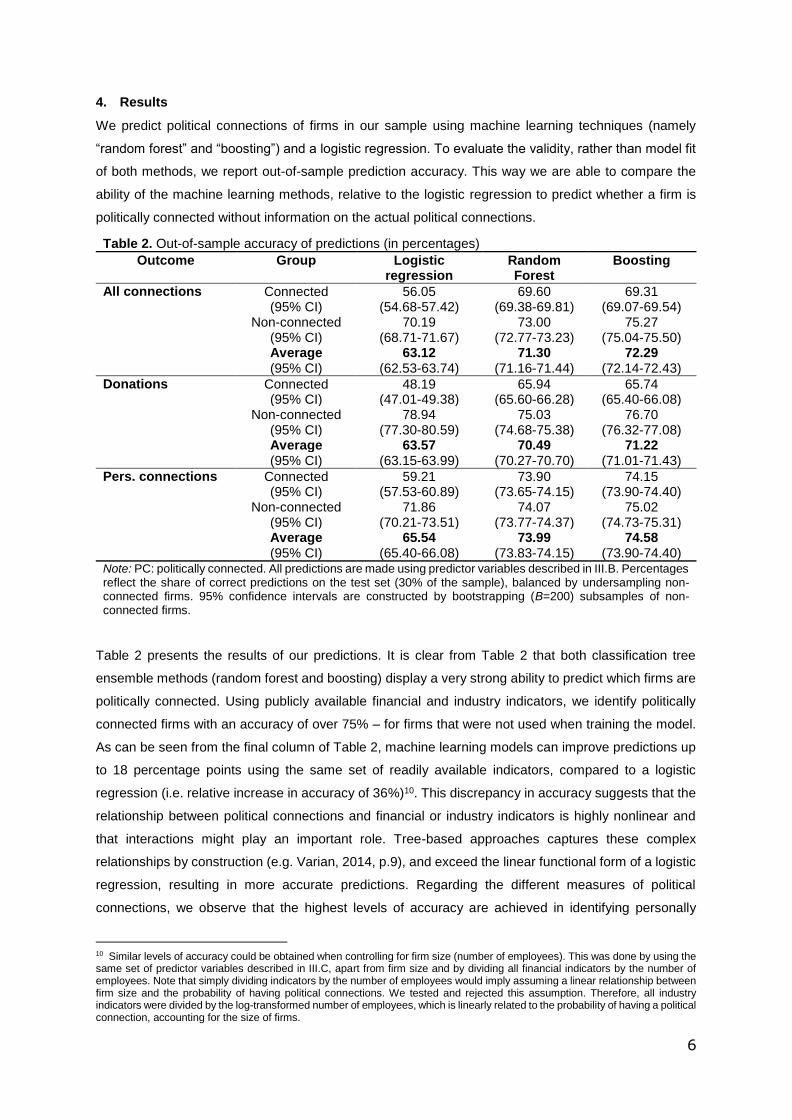
We predict political connections of firms in our sample using machine learning techniques (namely
“random forest” and “boosting”) and a logistic regression. To evaluate the validity, rather than model fit
of both methods, we report out-of-sample prediction accuracy. This way we are able to compare the
ability of the machine learning methods, relative to the logistic regression to predict whether a firm is
politically connected without information on the actual political connections.
Table 2 presents the results of our predictions. It is clear from Table 2 that both classification tree
ensemble methods (random forest and boosting) display a very strong ability to predict which firms are
politically connected. Using publicly available financial and industry indicators, we identify politically
connected firms with an accuracy of over 75% – for firms that were not used when training the model.
As can be seen from the final column of Table 2, machine learning models can improve predictions up
to 18 percentage points using the same set of readily available indicators, compared to a logistic
regression (i.e. relative increase in accuracy of 36%)10. This discrepancy in accuracy suggests that the
relationship between political connections and financial or industry indicators is highly nonlinear and
that interactions might play an important role. Tree-based approaches captures these complex
relationships by construction (e.g. Varian, 2014, p.9), and exceed the linear functional form of a logistic
regression, resulting in more accurate predictions. Regarding the different measures of political
connections, we observe that the highest levels of accuracy are achieved in identifying personally
10 Similar levels of accuracy could be obtained when controlling for firm size (number of employees). This was done by using the same set of predictor variables described in III.C, apart from firm size and by dividing all financial indicators by the number of employees. Note that simply dividing indicators by the number of employees would imply assuming a linear relationship between firm size and the probability of having political connections. We tested and rejected this assumption. Therefore, all industry indicators were divided by the log-transformed number of employees, which is linearly related to the probability of having a political connection, accounting for the size of firms.
Table 2. Out-of-sample accuracy of predictions (in percentages)
Outcome Group Logistic regression
Random Forest
Boosting
All connections Connected 56.05 69.60 69.31 (95% CI) (54.68-57.42) (69.38-69.81) (69.07-69.54) Non-connected 70.19 73.00 75.27 (95% CI) (68.71-71.67) (72.77-73.23) (75.04-75.50) Average 63.12 71.30 72.29 (95% CI) (62.53-63.74) (71.16-71.44) (72.14-72.43)
Donations Connected 48.19 65.94 65.74 (95% CI) (47.01-49.38) (65.60-66.28) (65.40-66.08) Non-connected 78.94 75.03 76.70 (95% CI) (77.30-80.59) (74.68-75.38) (76.32-77.08) Average 63.57 70.49 71.22 (95% CI) (63.15-63.99) (70.27-70.70) (71.01-71.43)
Pers. connections Connected 59.21 73.90 74.15 (95% CI) (57.53-60.89) (73.65-74.15) (73.90-74.40) Non-connected 71.86 74.07 75.02 (95% CI) (70.21-73.51) (73.77-74.37) (74.73-75.31) Average 65.54 73.99 74.58 (95% CI) (65.40-66.08) (73.83-74.15) (73.90-74.40) Note: PC: politically connected. All predictions are made using predictor variables described in III.B. Percentages reflect the share of correct predictions on the test set (30% of the sample), balanced by undersampling non-connected firms. 95% confidence intervals are constructed by bootstrapping (B=200) subsamples of non-connected firms.

7
connected firms and they tend to be the lowest for donating firms. In the worst case, the logistic
regression does not outperform random guess (where the chances would be 50/50). The two machine
learning techniques appear to be 10% more accurate which represents a 35% increase compared to
the logistic regression. Furthermore, the machine learning techniques also exhibit lower variance in the
prediction accuracy. Thus, using the same data, we can obtain better predictions of political connections
by using machine learning techniques rather than a logistic regression.
5. Results
This article introduced a machine learning approach to identify politically connected firms from firm
characteristics. Using a unique dataset of contractors from the Czech Republic, we find that publicly
available financial and industry indicators accurately predict over 75% of the political connections. This
level of accuracy is 36% higher compared to the accuracy of the logistic regression model used to
predict binary outcome variables. The reason for the discrepancy between a logistic regression model
and our machine learning approach can likely be attributed to the complex relationship between
connections and financial results, which is not properly modelled by the former technique.
Overall, we observe that the logistic regression is outperformed by both random forests and the boosting
method, using the same data and the same set of variables. By contrast, if we compare random forests
to boosting, the difference between the two machine learning techniques is not always statistically
significant. Lastly, we observe that the machine learning techniques exhibit lower variation in accuracy
levels than logistic regression, which makes them more reliable when applied to a new dataset (such
as in a different country).
We propose that our approach could be used by public institutions to identify firms whose political
connections could represent major conflicts of interests. A clear advantage of our approach is that it
can be used in other countries provided that there is a training dataset of connected firms available11.
The identified firms can be then audited by public authorities or nongovernmental organizations. Our
simulations suggest that boosting could identify political connections with about 75% accuracy. As such,
this approach would allow for more targeted inspection of companies with conflicts of interests.
11 For instance, Fisman (2001) or Baranek and Titl (2018) provide manually collected subsets of politically connected firms in Indonesia and the Czech Republic, respectively.

8
6. References
Antweiler, W., & Frank, M. Z. (2004). Is All That Talk Just Noise? The Information Content of Internet
Stock Message Boards. Journal of Finance, 59(3), 1259-1294.
Baranek, B., & Titl, V. (2018). Political Connections and Competition on Public Procurement Markets.
Unpublished Manuscript.
Blau, B. M. (2017). Lobbying, political connections and emergency lending by the Federal Reserve.
Public Choice, 172, 333-358.
Blumenstock, J. E. (2016). Fighting poverty with data: Machine learning algorithms measure and
target poverty. Science, 353(6301), 753-754.
Breiman, L. (2001). Random Forests. Machine Learning, 45(1), 5-32.
Breiman, L., Friedman, J. H., Stone, C. J., & Olshen, R. A. (1984). Classification and regression trees.
Monterey: Brooks/Cole Publishing.
Campos, N. F., & Giovannoni, F. (2007). Lobbying, corruption and political influence. Public Choice,
131(1-2), 1-21.
Chalfin, A., Danieli, O., Hillis, A., Jelveh, Z., Luca, M., Ludwig, J., & Mullainathan, S. (2016).
Productivity and Selection of Human Capital with Machine Learning. American Economic
Review, 106(5), 124-127.
Cingano, F., & Pinotti, P. (2013). Politicians at work: the private returns and social costs of political
connections. Journal of the European Economic Association, 11(2), 433-465.
Faccio, M. (2006). Politically Connected Firms. American Economic Review, 96(1), 369-386.
Fisman, R., & Wang, Y. (2015). The Mortality Cost of Political Connections. Review of Economic
Studies, 82(4), 1346-1382.
Fisman, R., Schulz, F., & Vikrant, V. (2014). The private returns to public office. Journal of Political
Economy, 122(4), 806-862.
Goldman, E., Rocholl, J., & So, J. (2013). Politically Connected Boards of Directors and The
Allocation of Procurement Contracts. Review of Finance, 17(5), 1617-1648.
James, G., Witten, D., Hastie, T., & Tibshirani, R. (2013). An Introduction to Statistical Learning. New
York: Springer.
Jean, N., Burke, M., Xie, M., Davis, M. W., Lobell, D. B., & Ermon, S. (2016). Combining satellite
imagery and machine learning to predict poverty. Science, 353(6301), 790-794.

9
Kleinberg, J., Lakkaraju, H., Leskovec, J., Ludwig, J., & Mullainathan, S. (2018). Human Decisions
and Machine Predictions. Quarterly Journal of Economics, 133(1), 237-293.
Lehne, J., Shapiro, J. N., & Vanden Eynde, O. (2018). Building connections: Political corruption and
road construction in India. Journal of Development Economics, 131, 62-78.
Mullainathan, S., & Spiess, J. (2017). Machine Learning: An Applied Econometric Approach. Journal
of Economic Perspectives, 31(2), 87-106.
Olson, M. J., Sarna, N., & Swamy, A. V. (2000). Governance and Growth: A Simple Hypothesis
Explaining Cross-Country Differences in Productivity Growth. Public Choice, 102(3-4), 341-
364.
Schiltz, F., Sestito, P., Agasisti, T., & De Witte, K. (2018). The added value of more accurate
predictions for school rankings. Economics of Education Review, 67, 207-215.
Sukhtankar, S. (2012). Sweetening the Deal? Political Connections and Sugar Mills in India. American
Economic Journal: Applied Economics, 4(3), 43-63.
Titl, V., & Geys, B. (2019). Political Donations and the Allocation of Public Procurement Contracts.
European Economic Review, 111, p. 443-458.
Varian, H. R. (2014). Big Data: New Tricks for Econometrics. Journal of Economic Perspectives,
28(2), 3-28.
Ward, F. (2017). Spotting the Danger Zone: Forecasting Financial Crises with Classification Tree
Ensembles and Many Predictors. Journal of Applied Econometrics, 32(2), 359-378.

10
Online Appendix A: Machine learning algorithms
This section provides more background on the models introduced in the paper. Online Appendix B
outlines the complete R code needed to apply these models. For a more comprehensive overview of
both technicalities and coding requirements, see James et al. (2013).
Regression tree
Estimating a single classification tree (Breiman, Friedman, Stone, & Olshen, 1984) with p predictors
boils down to implementing the pseudocode below on the predictor space, consisting of possible values
for components 𝑋1, 𝑋2, …, 𝑋𝑝:
1. Divide the predictor space into J distinct regions 𝑅1, 𝑅2,…, 𝑅𝐽 using recursive partitioning.
a. 𝑅𝑖 ∩ 𝑅𝑗 = ∅, ∀ 𝑖, 𝑗
b. Regions are chosen to minimize the RSS: ∑ ∑ (𝑟𝑖)²𝑖∈𝑅𝐽
𝐽𝑗=1 , with 𝑟𝑖 = 𝑦𝑖𝑗 − �̂�𝑅𝑗
2. Predict �̂�𝑅𝑗 for every observation that ends up in 𝑅𝑗.
Random Forest
The accuracy of predictions can be improved considerably by a bootstrap-based approach known as
“bagging”. This involves constructing several regression trees on subsamples of the dataset. Going one
step further, one can also subsample the number of variables considered at each split. This approach
is called a “random forest” and essentially de-correlates the trees, which improves the accuracy of
predictions even further (Breiman, 2001).
Boosting
The inverse of the random forest approach is to grow a tree sequentially, by fitting it to the residuals
and hence giving increasing weight to misclassified observations at each iteration. This approach is
coined boosting, and can be described by the following pseudocode:
1. Set 𝑓(𝑥) = 0, 𝑟𝑖 = 𝑦𝑖 , ∀𝑖
a. Use training data to fit a regression tree (𝑓𝑏(𝑥)) with s splits.
b. Add a shrunken version of the new tree to update 𝑓: 𝑓 ← 𝑓(𝑥) + 𝜆𝑓𝑏(𝑥)
c. Update residuals 𝑟𝑖 ← 𝑟𝑖 − 𝜆𝑓𝑏(𝑥𝑖)
2. Repeat steps 1.a-c. for each bootstrap iteration b,…, B
3. Output the boosted model: 𝑓(𝑥) = ∑ 𝜆𝐵𝑏=1 𝑓𝑏(𝑥)
Parameter Tuning and Model Validation
Classification trees and ensemble methods such as random forest and boosting can improve
predictive accuracy considerably, compared to conventional approaches (e.g. section V). The price to
pay for this improved accuracy is an increase in the number of parameters that needs to be chosen
when using a more advanced algorithm. For a single classification tree, the number of end nodes needs
to be chosen, or alternately, the minimal number of observations at each end node. Both parameters
capture the depth of the tree. When running a random forest, one also needs to set the number of trees,

11
the size of the subsample (percentage of the total dataset) used to build a tree at each iteration, as well
as the number of variables randomly drawn at each split for consideration (percentage of all variables
included in the model). For boosting, one needs to set the learning rate 𝜆 and the depth of the tree. In
the application at hand, we tuned parameters using k-fold cross-validation (k=10).
Figure A1 displays the procedure behind parameter tuning. It depicts how parameters were obtained
by cross-validation and model validation using a test set. For the sake of clarity, we illustrate this by
predicting firms’ political connections. In total, 2,865 firms were politically connected in the Czech
Republic in 2011. Considering the severe imbalance between politically connected firms and non-
connected firms, any algorithm can achieve high accuracy levels by always predicting the
overrepresented class. For example, in our case, when 3.45% of firms are politically connected, 96.55%
of firms will be correctly identified when firms are always predicted not to be politically connected.
Therefore, a new dataset needs to be constructed by rebalancing the class (i.e. connected and non-
connected firms). This is done in Step 1. At each iteration, a random sample is drawn from the sample
of non-connected firms. Hence, the sample used to build (train and test) the model (steps 2-4) will be
of size 5,730 in which half the firms are politically connected and half are not connected. Since this
random draw is repeated at each iteration, the results are not dependent one the composition of a single
sample (see below). Note also that all reported results are equivalent when an unbalanced test set is
used to compare the out-of-sample performance of different methods (see Footnote 9).
Once the data is balanced, the new dataset is split into a training and test set (Step 2). A conventional
split rule is to assign 70% to the training set, and 30% to the test set. As a result, 4,011 (0.7*5,730)
politically connected firms will be used to learn the relationships between firm and industry indicators
and political connections when building the classification trees (Step 3). The training set is first split into
10 folds of the dataset. Using 9 folds, the model is built and predictions are made on the 10th fold. This
process is repeated for every fold (10 times) and the cross-validation error (CVE) is computed as the
mean squared error on these 10th folds. This is done for a multitude of parameter combinations
(increasing computation time) and the final model is chosen as the one which minimizes CVE. Finally,
in Step 4, this final model is used to predict political connections for the remaining 1,719 firms
(0.3*5,730) by applying the learned rules. The resulting error rate is the out-of-sample error, since the
data used to validate the model was not used when constructing the classification trees.
Repeating steps 1-4 yields confidence intervals (CIs) for the out-of-sample errors, which allows us to
assess whether machine learning models are significantly better at identifying politically connected firms
when confronted with new data. We do this iteration 200 times, limited by computational power, as it
enables us to construct CIs at the 95% level.

12
Figure A1 : Model construction and validation, using training and test set.
Note: See text for interpretation.

13
Online Appendix B: Programming code in R # Change path to dataset setwd("C:/...") # Load packages library(haven) library(xgboost) library(ranger) library(data.table) library(caTools) library(caret) library(randomForest) set.seed(123) # Load data data<- < read dataset here > outcomes<-data.frame( < choose outcome variables to be predicted here >) predictors<-data.frame( < choose predictor variables here > ) output<-outcomes[ < j > ] # predict outcome j [1,2 or 3] model1<-data.frame(predictors, output) colnames(model1)[length(model1)]<-"output" model1_0<-subset(model1,model1$output==0) model1_1<-subset(model1,model1$output==1) ### Create matrix to save bootstrapped results (N = B) B=200 number_of_models=3 results<-matrix(data=NA, nrow = B, ncol = number_of_models*3) ### Start loop for (i in (1:B)) { # Repeatedly (B) draw subsamples model1_0sub<-model1_0[sample(nrow(model1_0), nrow(model1_1)),] model1_full<-rbind(model1_0sub,model1_1) # split into training and test sample = sample.split(model1_full$output, SplitRatio = .7) train1=subset(model1_full, sample==TRUE) test1 = subset(model1_full, sample==FALSE) #LOGISTIC results[i,1:3]<-logistic(train1,test1, output) #RANDOM FOREST results[i,4:6]<-rf(train1,test1,output) # XGBOOST results[i,7:9]<-boost(train1, test1,output) } summary(results) ### Define functions logistic <- function(train1, test1, output) { log = glm(formula = output ~ ., family = binomial, data = train1) prob_pred = predict(log, type = 'response', newdata = test1[-length(test1)]) prediction <- as.numeric(prob_pred > 0.5)

14
cmlog=table(test1$output,prediction) res_all<-(cmlog[1,1]+cmlog[2,2])/(length(prediction)) res_1<-cmlog[2,2]/(cmlog[2,1]+cmlog[2,2]) res_0<-cmlog[1,1]/(cmlog[1,1]+cmlog[1,2]) res<-cbind(res_all,res_1,res_0) return(res) } rf <- function(train1, test1, output) { x<-as.matrix(train1[,-length(train1)]) y<-as.matrix(train1[,length(train1)]) bestmtry <- tuneRF(x, y, stepFactor=1, improve=0.000001, ntreeTry=500) bestm<-bestmtry[which.min(bestmtry[,2])] RF = ranger(output ~ . , data= train1, mtry=bestm, num.trees=500, classification=TRUE, write.forest=TRUE) predict<-predict(RF, test1) prediction <- as.numeric(predict$predictions > 0.5) cmRF=table(test1$output,prediction) res_all<-(cmRF[1,1]+cmRF[2,2])/(length(prediction)) res_1<-cmRF[2,2]/(cmRF[2,1]+cmRF[2,2]) res_0<-cmRF[1,1]/(cmRF[1,1]+cmRF[1,2]) res<-cbind(res_all,res_1,res_0) return(res) } boost <- function(train1, test1, output) { label=as.numeric(train1[[length(train1)]]) table(label) dat=as.matrix(train1[-length(train1)]) xgmat=xgb.DMatrix(dat,label=label) best_param = list() best_seednumber = 123 best_auc=0 best_auc_index = 0 for (iter in 1:200) { param <- list(objective = "binary:logistic", eval_metric = "auc", max_depth = sample(6:10, 1), eta = runif(1, .01, .3), gamma = runif(1, 0.0, 0.2), subsample = runif(1, .6, .9), colsample_bytree = runif(1, .5, .8) ) cv.nround = 100 cv.nfold = 10 seed.number = sample.int(10000, 1)[[1]] set.seed(seed.number) mdcv <- xgb.cv(data=xgmat, params = param, nthread=6, nfold=cv.nfold, nrounds=cv.nround, verbose = T, early_stopping_rounds=10, maximize = TRUE, finalize=TRUE) max_auc = max(mdcv$evaluation_log$test_auc_mean) max_auc_index = which.max(mdcv$evaluation_log$test_auc_mean) if (max_auc > best_auc) { best_auc = max_auc best_auc_index = max_auc_index best_seednumber = seed.number best_param = param } }

15
nround = best_auc_index set.seed(best_seednumber) xgmat=xgb.DMatrix(dat,label=label) xgb <- xgb.train(data=xgmat, params=best_param, nrounds=nround, nthread=6) dat=as.matrix(test1[-length(test1)]) pred=predict(xgb, dat) prediction <- as.numeric(pred > 0.5) print(head(prediction)) cmXGB=table(test1$output,prediction) res_all<-(cmXGB[1,1]+cmXGB[2,2])/(length(prediction)) res_1<-cmXGB[2,2]/(cmXGB[2,1]+cmXGB[2,2]) res_0<-cmXGB[1,1]/(cmXGB[1,1]+cmXGB[1,2]) res<-cbind(res_all,res_1,res_0) return(res) }