identification of critical key performance indicators … · identification of critical key...

_________________________________________________________________________

Identification of Critical Key Performance Indicators for

Anglo Coal Underground Mining Operations

by

Madinoge Jeanette Maserumule s25310454

Submitted in partial fulfilment of the requirements for the degree of

BACHELOR OF INDUSTRIAL AND SYSYTEMS ENGINEERING

in the

FACULTY OF ENGINEERING, BUILT ENVIRONMENT AND INFORMATION

TECHNOLOGY

UNIVERSITY OF PRETORIA

October 2009 _________________________________________________________________________

ii

Executive summary�

The most essential task of any production company is to be able to manage production with

reliable methods developed using realistic data, thus creating a platform for continuous

improvement using forecasting methods that can predict the future given past data. The

objective of this paper is to study key performance indicators using statistical tools and

develop a model that can be used to identify a combination of key performance indicators

that are critical in terms of reaching production targets. Literature review was done to

highlight relevant tools, techniques and methods that can be used to develop an analysis

model that will reach the objectives of the project. This should aid Anglo Coal South Africa in

accelerated decision making capabilities utilising proposed solution strategies to achieve

stated business objectives.

iii

Acknowledgements

I wish to express my gratitude to people who through their contribution made this project

possible.

Thank you Mr. Derek Laing from Anglo Coal South Africa, Mr. Zaais Van Zyl, Mr. Gary Smith

and Mrs. Lauren Theron from Mining Consulting Services.

Additionally I would like to acknowledge the contribution of the following people:

Mr Olufemi Adentunji, for the reviews and provision of theoretical guidance. Andile Ndiweni

and Takalani Mudau for guidance and support.

iv

Contents

1. Introduction ..................................................................................................................... 1�

1.1Mining Process ............................................................................................................. 2�

1.2 Pick Six ....................................................................................................................... 3�

1.3 Problem Statement...................................................................................................... 6�

1.4 Research design and methodology ............................................................................. 7�

�

2. Literature review ............................................................................................................. 8�

2.1 Problem formulation .................................................................................................... 8�

2.2 Time series analysis .................................................................................................... 8�

2.2.1 Smoothing ............................................................................................................ 9�

2.3 Multiple regression analysis ........................................................................................ 9�

2.3.1 Least squares estimation .................................................................................... 10�

2.3.2 Partial ordinary least squares analysis................................................................ 10�

2.3.3 Sequential ordinary least square analysis ........................................................... 11�

2.4 Principal component analysis .................................................................................... 12�

2.5 Linear programming .................................................................................................. 12�

2.6 Excel model............................................................................................................... 13�

2.7 Conclusion ................................................................................................................ 14�

�

3. Multiple regression analysis ........................................................................................ 15�

3.1 Terminology .............................................................................................................. 16�

3.2 General structure ...................................................................................................... 16�

3.3 Statistical significance ............................................................................................... 21�

�

v

4. Computational Results ................................................................................................. 24�

4.1 Model outputs ............................................................................................................ 24�

4.2 Solution quality .......................................................................................................... 26�

�

5. Recommendations ........................................................................................................ 27�

5.1 Future work ............................................................................................................... 27

vi

List of figure

1.1: Shift breakdown…………...…………………………………………………………...……..…2

1.2: Components of a shift time………………………………………………………………..…...2

1.3: Mining process, cutting cycle flow chart……………………………………….….…….........3

1.4: KPI tree………………………………………………………………………..………………….4

1.5: Production process……………………………………………………………………………...5

2.1: Least squares estimation………………………………………………………….…….…....10

3.1: Studentised residual graph of the final model: Vlaaklagte-Simunye Section…...….…...23

vii

List of table

3.1: Regression terminology..................................................................................................16

3.2: ‘Pick six’ model symbols……………………………………………………………….......…17

4.1: Significant parameter estimates.................................................................................... 25

viii

Acronyms

ACSA Anglo Coal South Africa

CM Continuous miner

KPI Key performance indicator

SAS Statistical Analysis Software

Definitions

Continuous miner: remote-controlled machine with a large rotating steel drum equipped

with tungsten carbide teeth that scrapes coal from the seam.

Production time: production unit of a mine, where coal is mined

Shuttle car: electric powered vehicle with a capacity of 20 tons used to transport

coal from a mined seam to a section conveyor belt.

Sump: primary cutting motion of moving cutter head of CM into the coal face.

Tram: the movement process that a CM undergoes to cut coal

1

Part I

Introduction

Business organisations make use of key performance indicators (KPI’s) to measure the

success of production management and to define a suitable set of performance indicators for

monitoring ongoing performance. KPI’s are quantifiable measurements that reflect the

critical success factors of an organisation thus Anglo Coal South Africa (ACSA) has

identified and defined six key performance indicators referred to as the ‘Pick Six’ to manage

underground coal mining operations.

ACSA is a division of Anglo American and one of South Africa’s largest coal producers. It

operates four underground and five open cut mines in Mpumalanga, Witbank Coalfield. It is

well known for producing thermal and metallurgical coal to customers in the inland domestic

markets as well as the export market. ACSA’s coal demand has grown tremendously

inducing a need to improve production managing methods that can help with managing coal

operations, budgeting processes and forecasting tools to predict and lessen the risk of not

meeting coal demand.

A standard model has been built to assist in managing coal production using the ‘Pick Six’

and fixed mine parameters. With the aid of a third-party data capturing and management

company, Mining Consulting Services, data used to manage coal production is captured

daily using data cards that are attached to each operating Continuous miner during a

scheduled shift. A face shift report document is prepared daily using the mining data from

the previous day illustrating actual key performance indicators relative to the benchmarked

KPI’s, required production tonnes, production time etc.

The reports are used as

• a check tool to measure actual coal against budgeted coal targets and

• illustrate graphically the actual coal tonnes per day against the ‘Pick Six’ values

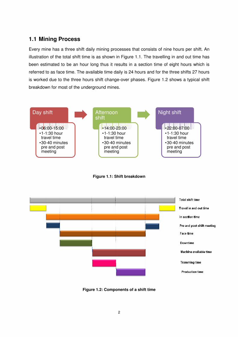
1.1 Mining Process

Every mine has a three shift daily mining

illustration of the total shift time is a

been estimated to be an hour long thus it results in a section

referred to as face time. The available

is worked due to the three hours shift change

breakdown for most of the underground mines.

Figure 1.

Day shift

•06:00-15:00•1-1:30 hour travel time

•30-40 minutes pre and post meeting

2

has a three shift daily mining processes that consists of nine

illustration of the total shift time is as shown in Figure 1.1. The travelling in and out time has

been estimated to be an hour long thus it results in a section time of eight

The available time daily is 24 hours and for the three shifts 27 hours

to the three hours shift change-over phases. Figure 1.2 shows a typical shift

breakdown for most of the underground mines.

Figure 1.1: Shift breakdown

Figure 1.2: Components of a shift time

Afternoon shift

•14:00-23:00•1-1:30 hour travel time

•30-40 minutes pre and post meeting

Night shift

•22:00•1-1:30 hour travel time

•30-pre and post meeting

hours per shift. An

in and out time has

time of eight hours which is

and for the three shifts 27 hours

Figure 1.2 shows a typical shift

Night shift

22:00-07:001:30 hour

travel time-40 minutes

pre and post meeting

3

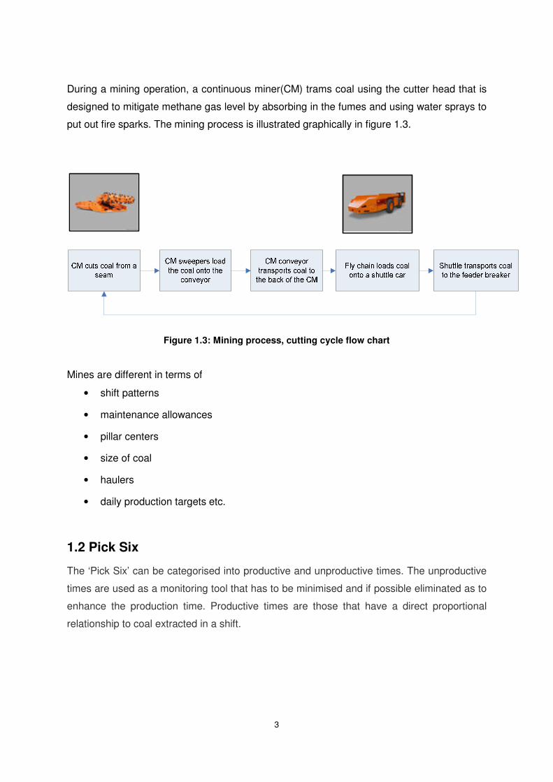
During a mining operation, a continuous miner(CM) trams coal using the cutter head that is

designed to mitigate methane gas level by absorbing in the fumes and using water sprays to

put out fire sparks. The mining process is illustrated graphically in figure 1.3.

Figure 1.3: Mining process, cutting cycle flow chart

Mines are different in terms of

• shift patterns

• maintenance allowances

• pillar centers

• size of coal

• haulers

• daily production targets etc.

1.2 Pick Six

The ‘Pick Six’ can be categorised into productive and unproductive times. The unproductive

times are used as a monitoring tool that has to be minimised and if possible eliminated as to

enhance the production time. Productive times are those that have a direct proportional

relationship to coal extracted in a shift.

4

Figure 1.4: KPI tree

Operational critical success factors for Anglo Coal for underground operations are to;

• achieve planned coal production targets in order to meet customer demand

• operate mining equipments efficiently by reducing the machine idle time

Critical factors are only achievable if the KPI’s benchmarked values are reliable and their

effect on the coal production tonnes is well understood. The three past projects defined and

reviewed the KPI’s to ensure that Anglo Coal has a coal managing standard that can be

deployed in all the underground mines. [3][6][11] The KPI’s are explained as follows;

First sump late

It is the time difference between the scheduled start of a shift and the first sump that

the CM makes. It decreases the face time available during a shift by the same

amount of minutes the shift started late.

*Measurement unit: Minutes

Load time

The total time a CM takes to fill up a shuttle car or battery loader with coal. It makes

up the production process together with the away time as depicted in figure 1.5. It is

calculated by the following formula per shift;

��

Load timeProductive times

Away time

Tram time per meter cut

Pick Six

First sump lateUnproductive times

Last sump early

Downtime

5

*Measurement unit: seconds

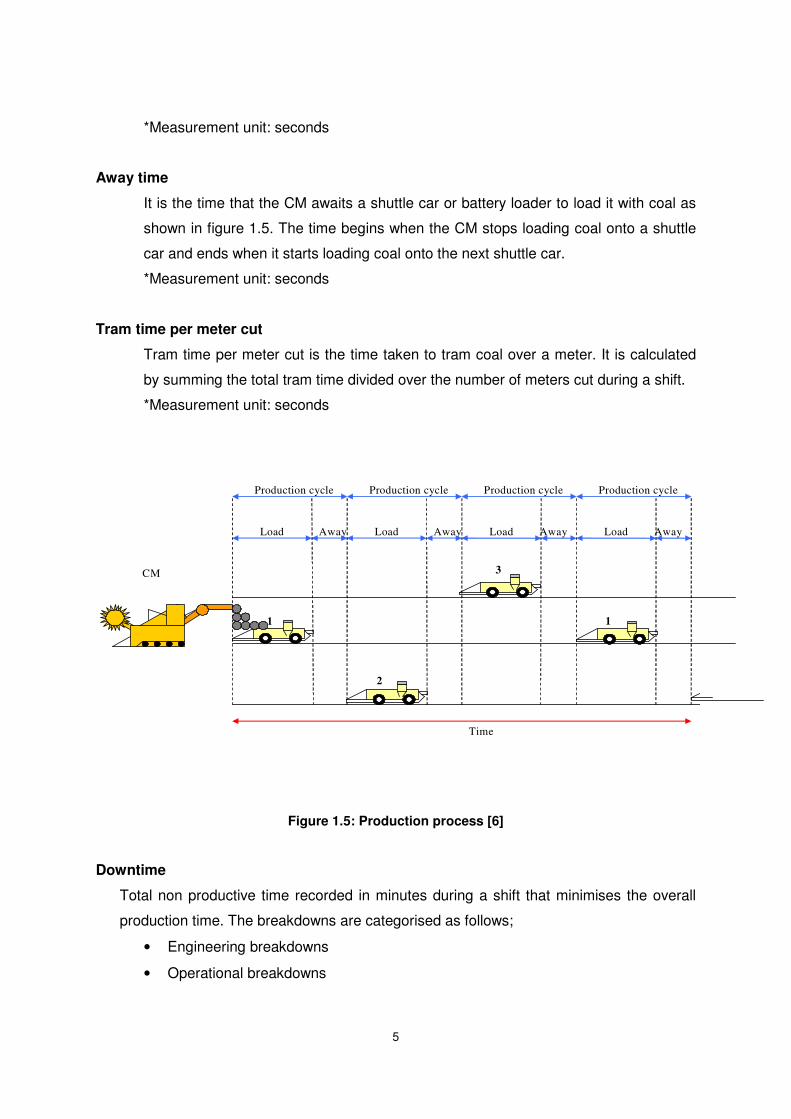
Away time

It is the time that the CM awaits a shuttle car or battery loader to load it with coal as

shown in figure 1.5. The time begins when the CM stops loading coal onto a shuttle

car and ends when it starts loading coal onto the next shuttle car.


Tram time per meter cut

Tram time per meter cut is the time taken to tram coal over a meter. It is calculated

by summing the total tram time divided over the number of meters cut during a shift.


Figure 1.5: Production process [6]

Downtime

Total non productive time recorded in minutes during a shift that minimises the overall

production time. The breakdowns are categorised as follows;

• Engineering breakdowns

• Operational breakdowns

Production cycle Production cycle

Away Away Away Away Load Load Load Load

Production cycle Production cycle

2

1

3

1

Time

CM

6

• Sectional conveyor breakdowns

• Trunk conveyor breakdowns

• Other


Last sump early

The time difference between the planned end of a shift and the last sump the CM

makes. The KPI time decreases the face time available during a shift.


The ‘Pick Six’ is used to calculated figures such as the following that can be used to

calculate the actual coal production per shift.

• production time

�� !�� "�� !#��

• Average production rate

$%&&'��( � �)��( �"�� *�"��"��+�, -.+��'��"��*��)

1.3 Problem Statement

Each KPI is evaluated individually without any comparison to the other KPI’s as to which

one(s) has the highest impact on coal production target. This gives minute results as to how

the KPI’s can be collectively utilised to the maximum in order to make better operational

decisions. ACSA requires a combination of KPI’s that are significant for reaching coal

production targets.

7

1.4 Research design and methodology

Past and present similar projects were studied as to adapt the methodology and obtain the

solution strategy using such methods. Such projects have been performed mostly in the

financial, biological, medical environments and all had a common solution strategy which is

to predict the response variable using KPI’s, in this instance the coal production tonnes per

shift/day.

The first phase focused on identifying a solution strategy technique that can be used to

identify a set of KPI’s. Using KPI information obtained from the Mining Consulting Services,

the best technique was selected for the identification process of critical KPI’s.

The second phase focused on the solution strategy formulation based on the selected

technique to determine the KPI combination. Data was extracted from excel and all the

necessary computations were performed as to achieve the desired end goals. The model

was inputted with all the different mines data.

For the third phase, computational results for each mine were studied and compared to the

other mines. In the case of uncertainties, the model outputs were reviewed as to get an in-

depth understanding of the uncertainties. This was mostly due to the fact that some of the

mines characteristics differed.

8

Part II

Literature review

The problem should be defined in such a way that each KPI can be analysed both

individually and collectively with the other KPI’s. As mentioned before, each KPI is used to

calculate the production time and thus there exists a relationship between the KPI’s and the

actual coal tonnes mined. These relationships will not be considered imperative for

technique selection, however they will only be considered where applicable.

2.1 Problem formulation

Looking at the objectives of the study, the problem can be formulated in such a way that the

KPI’s will be used or tested as to yield maximum coal production tonnages. The ‘Pick Six’

will be classified as independent variables where X={X1,...,X6} denotes the KPI set. The coal

production tonnages will be classified as the dependent variable.

2.2 Time series analysis

Time series analysis entails analysis of a sequence of measurements made at specified time

intervals. The two main goals of time series analysis [14]:

• Identifying the nature of the phenomenon represented by the sequence of

observations,

• forecasting i.e. predicting future values of the time series variable

Both of these goals require that the pattern of the observed time series data be

identified and more or less formally described. Interpretation and integration can be made

once a pattern has been identified with the other data i.e., use it in the theory of the

investigated phenomenon, e.g., seasonal death rates. Extrapolation of the identified pattern

can be made as to predict future events.

9

2.2.1 Smoothing

Smoothing method uses the averaging methods and exponential smoothing methods to

reveal clearly the underlying trend, seasonal and cyclic components from data sets. The

methodology behind smoothing methods is taking the averages of the data sets and

analyzing the data using the following;

• the mean squared errors

• sum of the squared errors

• mean of the squared errors

The above mentioned can be derived from a built forecasting model that when analysed, the

‘Flaw of averages’ is sometimes checked for in the model. What the ‘Flaw of averages’

states is that plans based on the assumption that average conditions will occur are usually

wrong.

2.3 Multiple regression analysis

The basic purpose of a statistical investigation is to make predictions and optimise by

determining what values of the independent variable/s is the dependent value a maximum or

minimum. [5] Multiple regression analysis is a flexible method of data analysis that is

appropriate whenever a quantitative (response) variable is to be examined in relationship to

any predictor variable and regression analysis is most widely used for such functions. The

basic regression formula is as follows;

) /0�� ( /1��21 (3( /�4��24 ( 5��6789:

Where

y = dependent variable

x = independent variable

E(y) = deterministic component

� = random error component

�0 = y-intercept of the line, i.e. point at which the line cuts through the y-axis

�1 = slope of the line, i.e. amount of increase in the mean of y for every 1-unit

increase in x.

2.3.1 Least squares estimation

The regression coefficients,

squares of which the coefficients minimises the error sum of squares

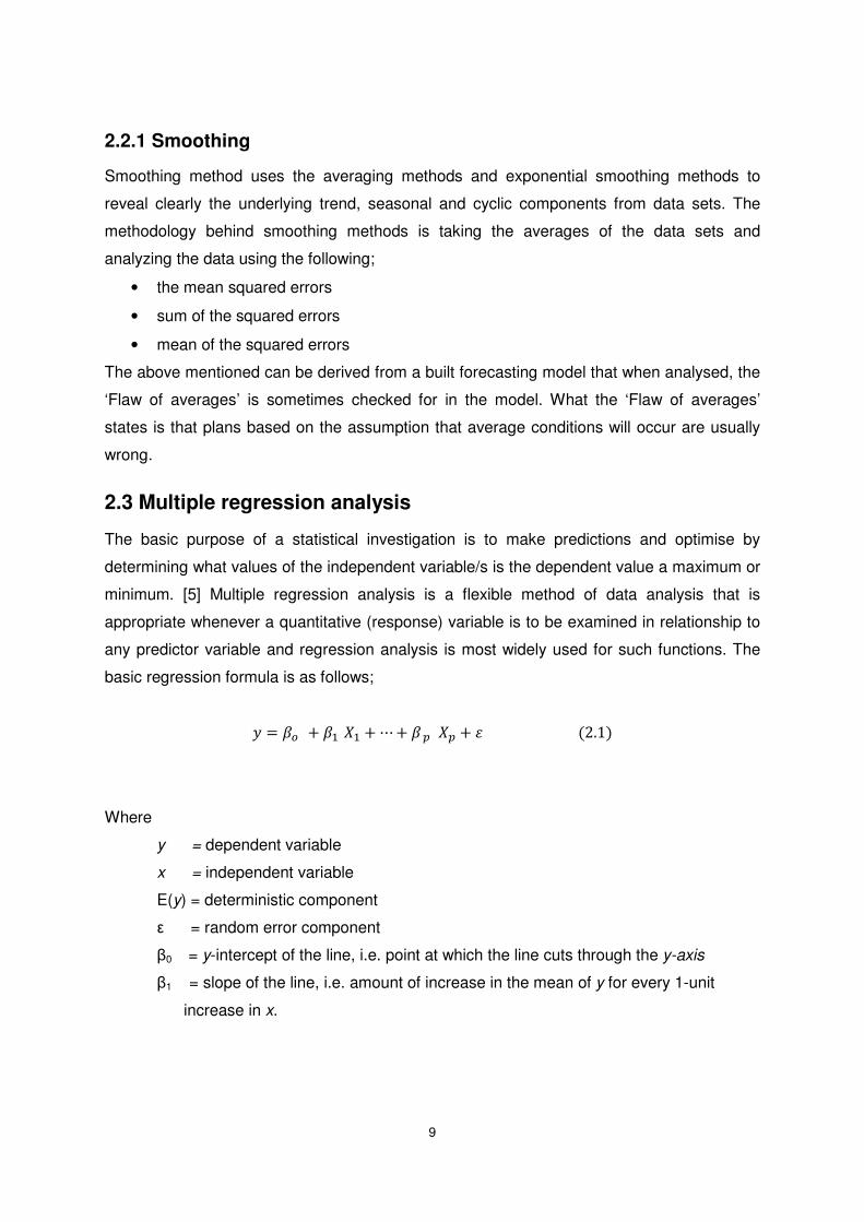
This means the distance between the

the actual Y values denoted by

referred to as the residual or prediction error

For a test to be accurate, certain assumptions have to

• data is sampled randomly and independently from the population

• and the deviations of the

distributed with equal variance for all predicted values of

Figure 2.

2.3.2 Partial ordinary least square

Randall D. Tobias [12] defines partial least square as a method for constructing predictive

models when the factors are many and highly collinear.

does is show how much a predictor improves

all the predictors, ‘Pick six’, it

squares. The regression sum of squares is a variati

of Y predicted by the predictor variable/s.

10

Least squares estimation

,. . . , are estimated using the method of

squares of which the coefficients minimises the error sum of squares

This means the distance between the fitted line which consists of the predicted

actual Y values denoted by asterisks in figure 2.1 is being minimised. This

residual or prediction error.

For a test to be accurate, certain assumptions have to be satisfied [1]

data is sampled randomly and independently from the population

the predicted values from the actual Y values are normally

distributed with equal variance for all predicted values of

Figure 2.1: Least squares estimation

least squares analysis

defines partial least square as a method for constructing predictive

s are many and highly collinear. Essentially what partial least square

predictor improves over all the other predictors. If it is added

, it will be defined as the increase in the regression sum of

squares. The regression sum of squares is a variation analysis of Y that show

of Y predicted by the predictor variable/s.

ordinary least

consists of the predicted values and

is being minimised. This distance is

from the actual Y values are normally

defines partial least square as a method for constructing predictive

Essentially what partial least square

over all the other predictors. If it is added over

defined as the increase in the regression sum of

shows the variation

11

The total variation is measured by the following formula;

;��'�-+� ��-<+�"�- =6>? ( >@:A��678$:B

?

And the variation that can be predicted is measured as follows;

C�#"�--��!�-+� ��-<+�"�- �=6>DE ( >@:AB

?��678F:

The residual sum of squares is measured as follows;

C�-��+�'��""�"�-+� ��-<+�"�- �=6>? � >DE:AB

?��678G:

Emphasis is put on the fact that the predictive models are used for predicting the responses

and also on trying to understand the underlying relationship between the explanatory

variables.

2.3.3 Sequential ordinary least square analysis

Sequential least square analysis shows how parameter predictions are improved as more

predictor variables are added in a defined order. The same concept of the increase in sum of

squares as explained under partial least square analysis is the same for sequential least

square analysis and equations 2.3, 2.4 and 2.5 were used. It is beneficial to use sequential

least square analysis if there is a natural order of the predictor variables.

From figure 1.3, the only order that can be distinguished is that the load time has to occur

before the away time. For the sumps KPI’s, the first sump late has to occur before the last

sump early and all the other KPI’s occur in between the two. This will not have any effect on

the integrity of the model if not followed as the KPI measurements are deemed independent.

Downtime can occur without any of the KPI’s could occur such as the loading of coal onto a

shuttle car.

12

2.4 Principal component analysis

Principal component analysis (PCA) is a widely used multivariate method that is seen and

described as a “complementary statistical’ method used to run rough preliminary

investigations, to sort out ideas, to put a new light on problem, or to point out aspects which

would not come out in a classical approach.”[9] The main objectives of PCA that are in line

with the problem at hand are; dimensionality reduction, feature selection i.e. the selection of

the most useful variables, identification of underlying variables. [9]

In terms of analysing large data subsets, PCA is a great tool due to its condensing of

information. If all mines KPI’s are to be analysed for trends, it will aid in enhancing the

chances of producing useful results.

2.5 Linear programming

A mathematical model can serve a number of purposes. The first function is that a

mathematical model can serve in regards to production as a tool for prediction. The types of

models that can be used are the descriptive mathematical models and simulation models. A

descriptive model can be used to predict the consequences of increasing a KPI value, that

is, the effect on coal production tones. With a simulation model, it can be used to predict the

outcome of prescribed set of strategies so as to provide needed input-output information to

solve a decision problem.

Secondly, it can be used as a tool for control or decision-making purposes. Decision

problems regarding controllable aspects of a process influence the operation of the process

by changing or controlling the value of some decision variable. The type of decision models

are modeled as to find the values of the decision variables that

• satisfy all constraints simultaneously

• achieve the stated objective

The methodology followed in generating a mathematical model fits perfectly with the

methodology planned for developing the solution strategy for the KPI identification process.

However, problems arise when generating the algorithm as known KPI production tonnes

relationships will be used thus the productive KPI’s that have a direct relationship to the

production tones will be favored.

13

For an example, the first sump late, last sump early and downtime KPI’s are merely

subtracted from the face time unlike the other KPI’s that are included in the production time

calculations used to calculate the actual coal produced in a shift/day.

2.6 Excel model

The modern trend in programming applications is graphical interfaces. This means that the

user interacts with a program through a graphical interface e.g. values are entered in text

boxes, options are selected from graphical menus and answers are presented graphically.

Excel macros are an option in terms of their ability to create options that can be selected

from a button etc. The macros are stored as VBA code that uses an ActiveX interface to

cause excel’s applications to perform actions such as change formulas, create charts etc.

The type of action that the application supports are defined by what is called an object

model.

The model was built by excel designers to provide an interface so that the programming

language can cause the application to do what a user normally would do interactively with a

mouse and keyboard. It includes the following:

• list of application objects that can be managed

• properties of these objects that can be examined or altered; in the coal production

model the value of the KPI’s can be altered.

• methods that can be performed on the object

An excel model can be embedded with calculations and measured values to output the

desired end goals. Using this tool all the requirements can be met using defined formulations

with the use of macros to show each KPI effect on the total coal tonnes. Each KPI factor can

be calculated which can easily be viewed on the excel spreadsheet. Further formulation can

be made using the KPI factors to select a combination of KPI that are critical in order to

reach budgeted coal production tones.

14

2.7 Conclusion

From the different techniques studied, it was deemed multiple regression analysis is the

most appropriate as it can yield the accurate required solution; however multiple regression

has been extensively used in medical fields than engineering fields when dealing with

variable selection studies. The other methods give rise to more problems as the solution

formulation gets complicated due to extensive computations that defeats the purpose of the

study. Due to the availability of software’s that can perform statistical computations,

Statistical Analysis Software (SAS) was the prominent in terms of usage and simplicity

understanding. The partial ordinary least square regression analysis methods will be used as

it is considered to yield accurate solution outcomes.

15

Part III

Multiple regression analysis

Multiple regression analysis is widely used in the psychology, dietary, population and

financial fields for prediction purposes. The relationship between the predictor variables and

response variable will be analysed as to determine which predictor variable/s has the most

impact on the response variable.

The following are the model assumptions as explained by Mendenhall for a regression

model [7]

Assumption 1: The mean of the probability distribution of � is 0 i.e. the average of the errors

over an infinitely long series of experiments is 0 for each setting of the

independent variable x.

Assumption 2: The variance of the probability distribution of � is constant for all settings of

the independent variable x.

Assumption 3: The probability of � is normal

Assumption 4: The errors associated with any two different observations are independent i.e.

the error associated with one y has no effect on the errors associated with

other y values.

A test for residual normality is crucial before any inferences can be made from the model.

The p-value [table 3.1] can only be used if the residual normality test is satisfied, if not

transformations are made and explained before using the p-value for parameter selection.

Test for normality

H0 : Residual come from a normal distribution

H1 : Residual deviate from a normal distribution

Shapiro-Wilk test

n� 50

Reject H0 if W Is small

p-value = p(w)< 0,05 : deviate from normal

>0,05: H0 is not rejected

16

A Shapiro-Wilk test is used only when the number of observation is less or equal to 50. The

rule of thumb is used for the confidence level i.e. � = 0,05 unless stated otherwise due to

failure to comply with normality tests. Data transformations are performed on the y values as

to make them nearly satisfy the assumptions, and for the latter reason, to achieve a model

that provides a better approximation to E(y).

3.1 Terminology

The basic terminology presented in part II; section 2.2 will be used with the additional

terminology explained in table 3.1 throughout the rest of the document.

Table 3.1: Regression terminology

Least square: Squared distance between the data points and the model.

The aim is to minimise the distance as to get a best fit

linear graph.

R-square: It measures how much of y, response variable is explained

by x, predictor variable

P –value: In statistical hypothesis testing, the p-value is the

probability of obtaining a test statistic at least as extreme

as the one that was actually observed, assuming that the

null hypothesis is true. The fact that p-values are based on

this assumption is crucial to their correct interpretation.

3.2 General structure

The steps applicable for developing a regression model are as listed below. Collection of

data and variable classification was done in Step 1 and 2. From the code written for the

model with the required output formulation for step 3, 4 and 5, the computations were done

simultaneously. Step 6 calculations are for validation. The model was stopped when the t-

test was not violated i.e. the p-value was less than 0.005.

17

Regression Analysis steps

Step 1: Collection of data for each experimental unit in the sample

Step 2: Variable classification

Step 3: Estimation of the unknown parameters, �0 , �1 , . . ., �6.

Step 4: Estimation of the probability distribution of the random error component � and its

variance

Step 5: Evaluation of the utility of the model

Step 6: Validation of assumptions on � and make model modifications if necessary

Step 7: If the model is deemed adequate, estimate the mean value of Y , identify the critical

KPI and make other inferences.

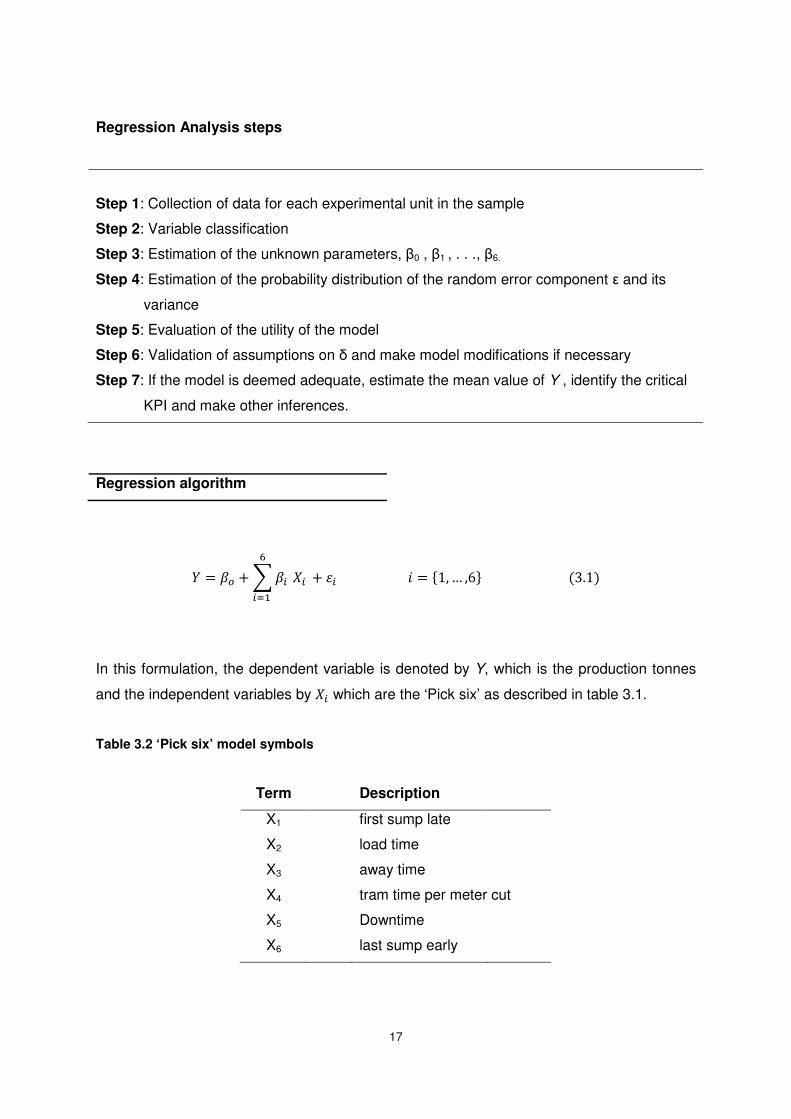
Regression algorithm

> /0 (=/?��2?�H

?I1�( 5? �� J9KL K%M��6$89:

In this formulation, the dependent variable is denoted by Y, which is the production tonnes

and the independent variables by 2? which are the ‘Pick six’ as described in table 3.1.

Table 3.2 ‘Pick six’ model symbols

Term Description

X1 first sump late

X2 load time

X3 away time

X4 tram time per meter cut

X5 Downtime

X6 last sump early

18

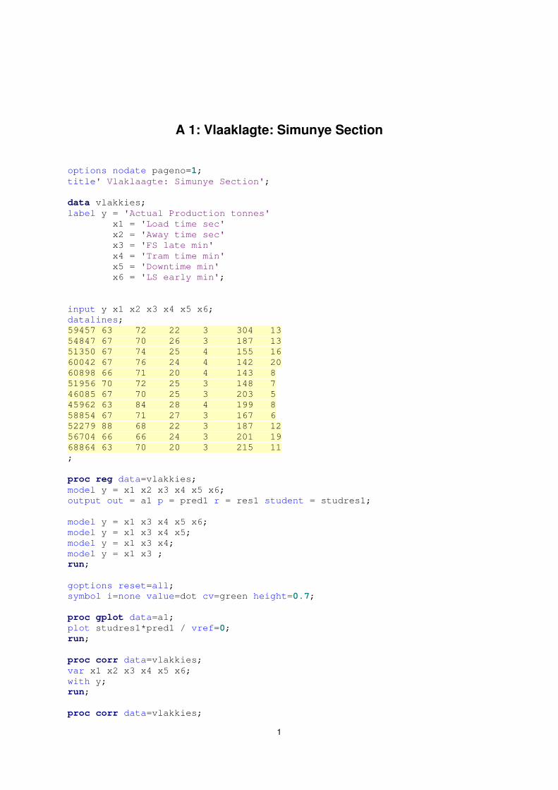
SAS algorithm

The model explained here is for one mine section, a couple of other models were run as to

accomplish a general KPI combination that can be used for all Anglo Coal underground

mining processes.(Addendum A and B)

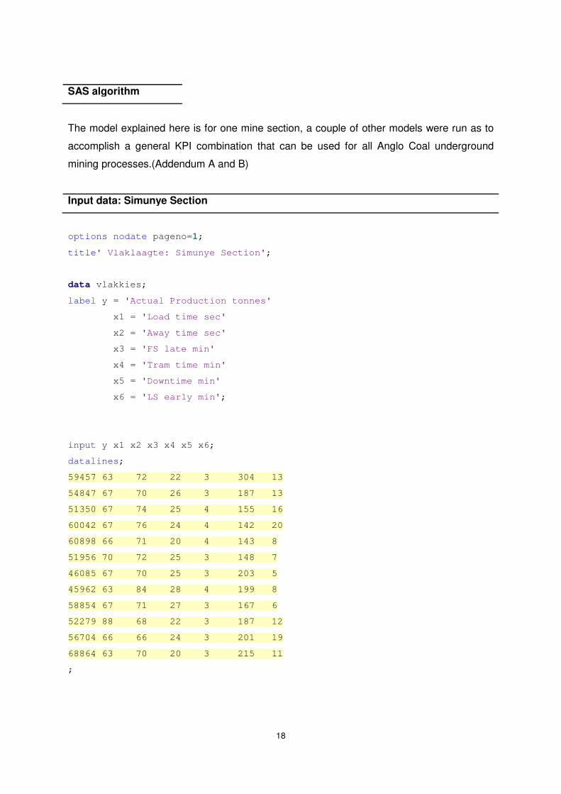
Input data: Simunye Section

options nodate pageno=1;

title' Vlaklaagte: Simunye Section';

data vlakkies;

label y = 'Actual Production tonnes'

x1 = 'Load time sec'

x2 = 'Away time sec'

x3 = 'FS late min'

x4 = 'Tram time min'

x5 = 'Downtime min'

x6 = 'LS early min';

input y x1 x2 x3 x4 x5 x6;

datalines;

59457 63 72 22 3 304 13

54847 67 70 26 3 187 13

51350 67 74 25 4 155 16

60042 67 76 24 4 142 20

60898 66 71 20 4 143 8

51956 70 72 25 3 148 7

46085 67 70 25 3 203 5

45962 63 84 28 4 199 8

58854 67 71 27 3 167 6

52279 88 68 22 3 187 12

56704 66 66 24 3 201 19

68864 63 70 20 3 215 11

;

19

Data points for each mine section were extracted from an excel spreadsheet and defined as

variables as in line 4(input) of the model algorithm. For this algorithm Simunye’s data was

tested using 12 data points.

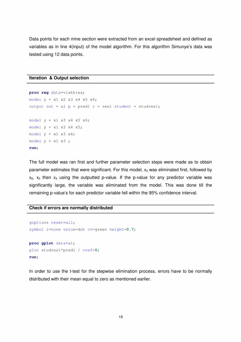
Iteration & Output selection

proc reg data=vlakkies;

model y = x1 x2 x3 x4 x5 x6;

output out = a1 p = pred1 r = res1 student = studres1;

model y = x1 x3 x4 x5 x6;

model y = x1 x3 x4 x5;

model y = x1 x3 x4;

model y = x1 x3 ;

run;

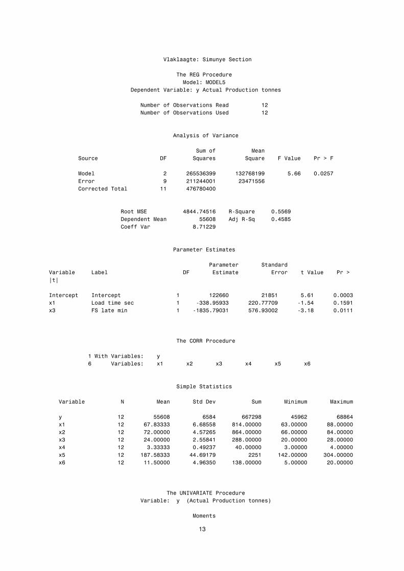
The full model was ran first and further parameter selection steps were made as to obtain

parameter estimates that were significant. For this model, x2 was eliminated first, followed by

x6, x5 then x4 using the outputted p-value. If the p-value for any predictor variable was

significantly large, the variable was eliminated from the model. This was done till the

remaining p-value’s for each predictor variable fell within the 95% confidence interval.

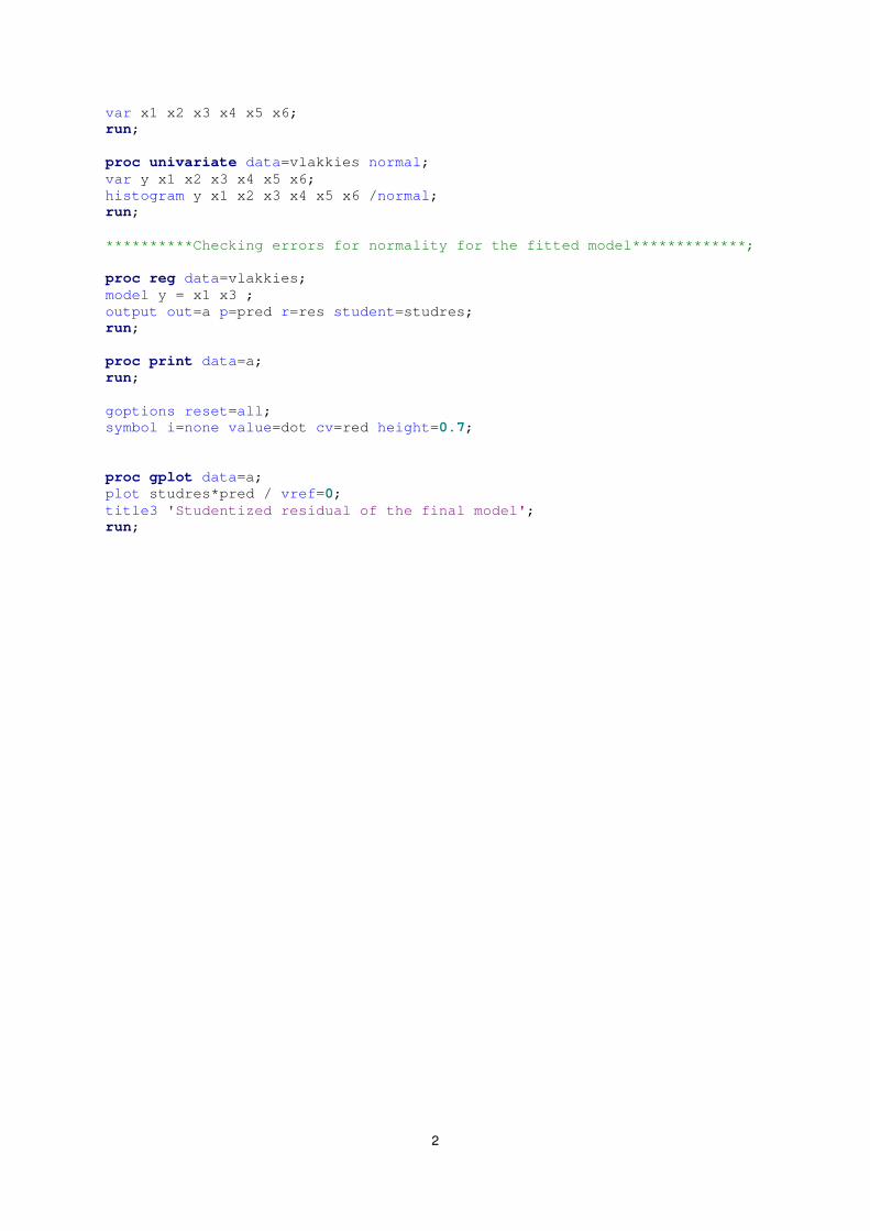
Check if errors are normally distributed

goptions reset=all;

symbol i=none value=dot cv=green height=0.7;

proc gplot data=a1;

plot studres1*pred1 / vref=0;

run;

In order to use the t-test for the stepwise elimination process, errors have to be normally

distributed with their mean equal to zero as mentioned earlier.

20

Check for correlation between the x variables and y

proc corr data=vlakkies;

var x1 x2 x3 x4 x5 x6;

with y;

run;

This checks for how y and x’s are related i.e. for example if there is a negative relationship

between y and one of the x values, take for instance the away time, the expected actual

production tonnes will decrease as the away time increases.

Check for correlation between the x variables

proc corr data=vlakkies;

var x1 x2 x3 x4 x5 x6;

run;

This was used to check for relationships between the x’s themselves. If highly correlated

predictor variables are present in the model, the results may be confusing. In some cases

the t test on the individual parameter estimates may be non-significant even though the F-

test for the overall model adequacy is significant and the parameter estimates may have

signs opposite from what is expected. Variation inflation factors aid in determining whether a

serious multicollinearity problem exists.

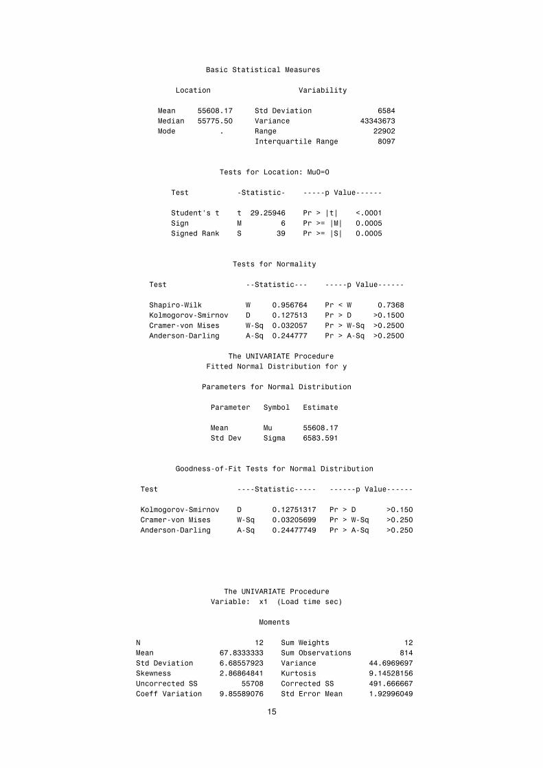
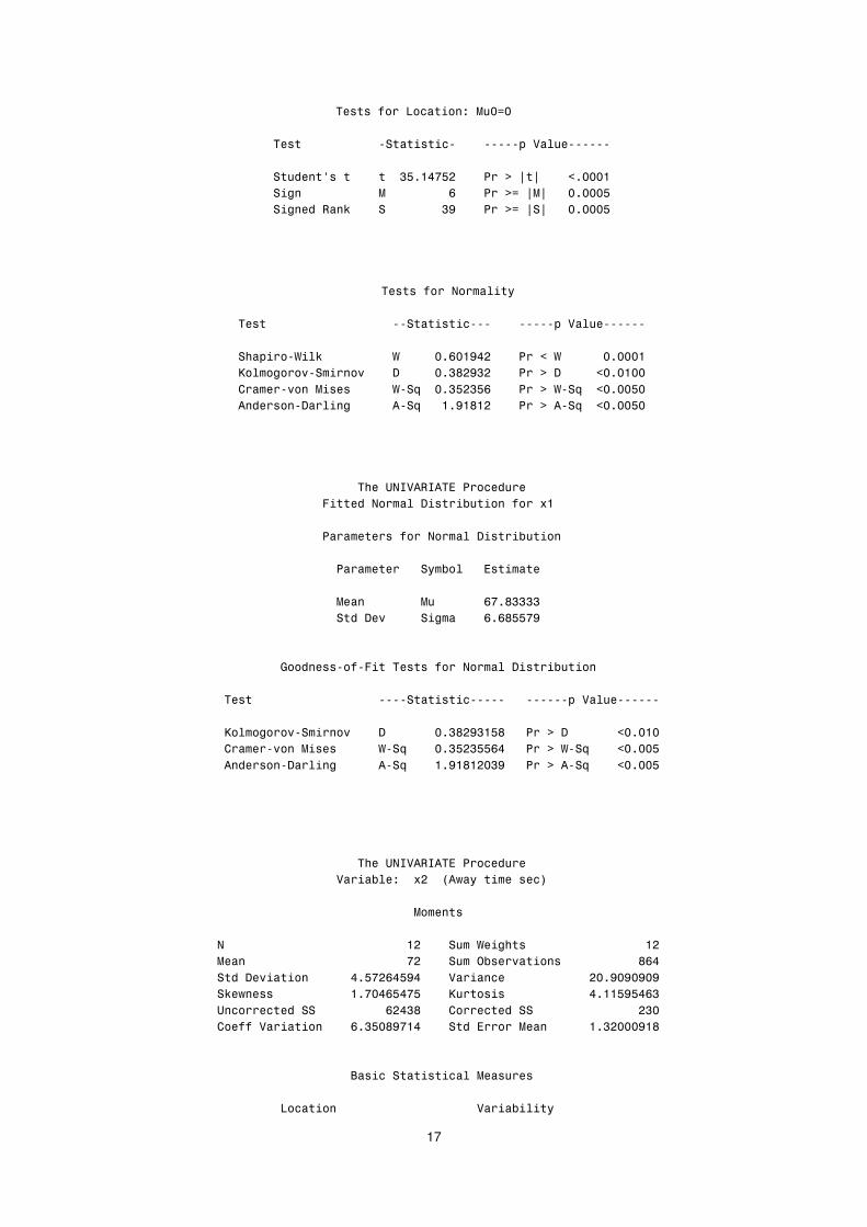
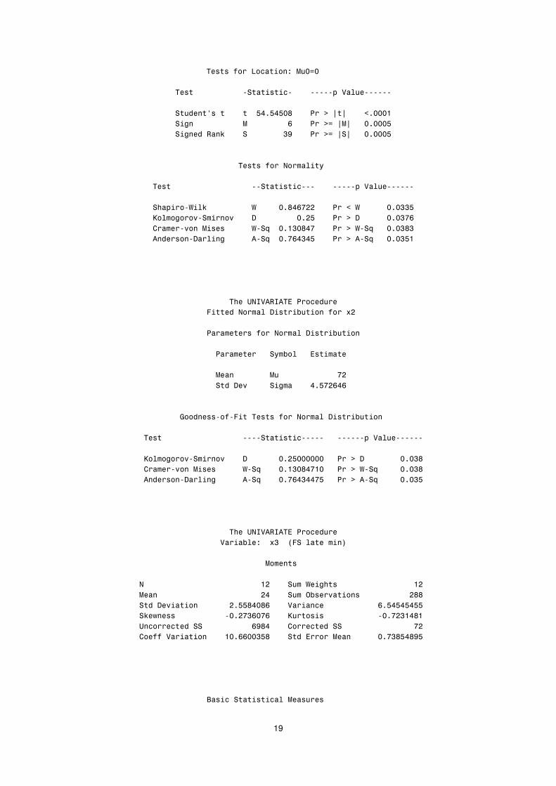
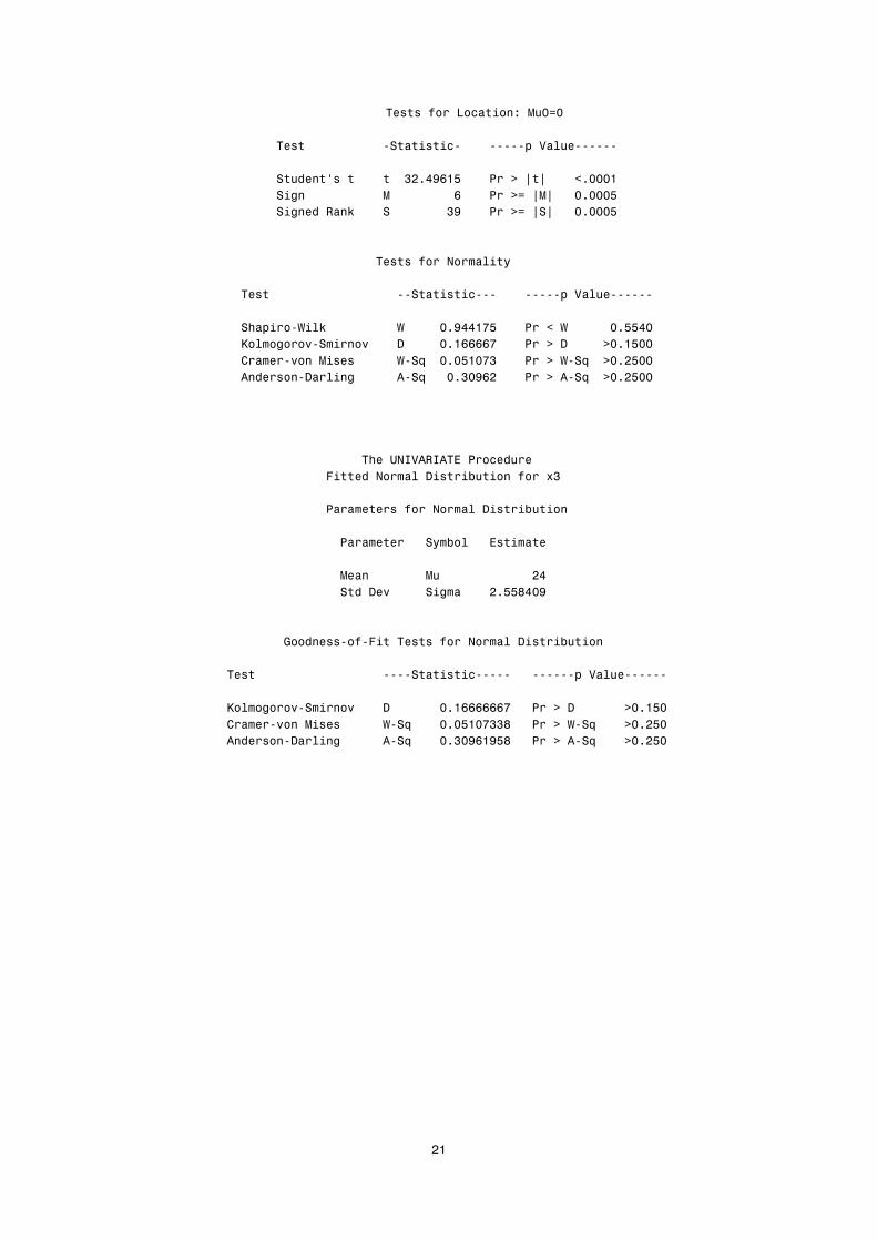
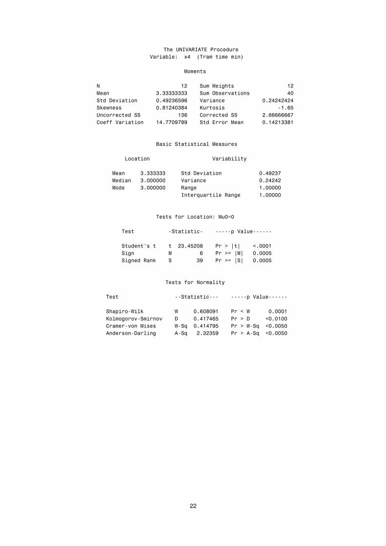
Data Normality Test

proc univariate data=vlakkies normal;

var y x1 x2 x3 x4 x5 x6;

histogram y x1 x2 x3 x4 x5 x6 /normal;

run;

The data normality test was to check if some KPI’s data were normally distributed. The

sample size was too small, i.e. less than 50 datasets thus it was infrequent for normality to

be observed in the datasets.

21

Fitted model for significant KPI’s

proc reg data=vlakkies;

model y = x1 x3 ;

output out=a p=pred r=res student=studres;

run;

proc print data=a;

run;

goptions reset=all;

symbol i=none value=dot cv=red height=0.7;

proc gplot data=a;

plot studres*pred / vref=0;

title3 'Studentized residual of the final model';

run;

This ensures that the errors are normally distributed as to satisfy the error normality

assumptions mentioned before. From the graph it can be seen that some of the errors do

come from a normal distribution or are normally distributed. (Refer to figure 3.1)

3.3 Statistical significance

A number of the models output will answer and show how reliable the solution strategy is.

The following are some of the important outputs that were studied;

R2: It provides a measure of how well Y can be predicted from the set of x scores i.e. the

amount of the total variation in Y that can be explained by x.

Adjusted R2: Is the same as the R 2 however it takes into account the number of

parameters being modeled, x. A high R2 portrays the reliability of a model in terms of

how much of the dependent variable is explained by the independent variables

Hypothesis testing: This aid in testing the validity of the estimated value of a parameter

and the utility of the model. By the rule of thumb, the significance level was defined to

be 5% but for the Vlaaklagte, Simunye Section, 20% was used only for testing the

22

parameters. If parameter estimates fell within the significance level, the null

hypothesis was rejected, stating that the parameters were significant from zero and if

not, stepwise regression was used to eliminate the parameters that were not

significant. The model was run until we had only significant parameters in the model.

This can be viewed in the iteration and output step of the SAS algorithm. X6 was

eliminated first followed by x5 and x4 consecutively.

F-test: The test is done on the full model using the F test for all the predictor variables

except for the intercept values as they have no significance on the solution strategy.

The null hypothesis can be rejected if the p-value is less than the � value.

Test for overall model significance

H0 : Model not significant

H1 : Model significant

� =0.05

Reject H0 if p-value is less than 0.05

T-test: Same test as the F-test but only done for parameter estimates.

Test for parameter significance

H0 : �i =0(Not significantly different from zero)

H1 : �i �0 (significantly different from zero)

� =0.05*

Reject H0 if p-value is less than 0.05

* Only 20% significance level was used for one (Vlaaklagte: Simunye Section) model as to

accommodate the actuality of not having sufficient data points.

The model has to be run in such a way that all the regression analysis assumptions are not

violated using the normality tests for errors. In order to use the p and f-test, normality for

errors must not be violated as the tests can only be used if the assumptions are met. If

normality is violated, then the model did not pass to merit for further considerations.

23

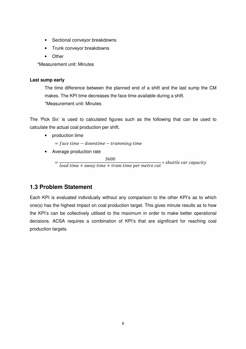
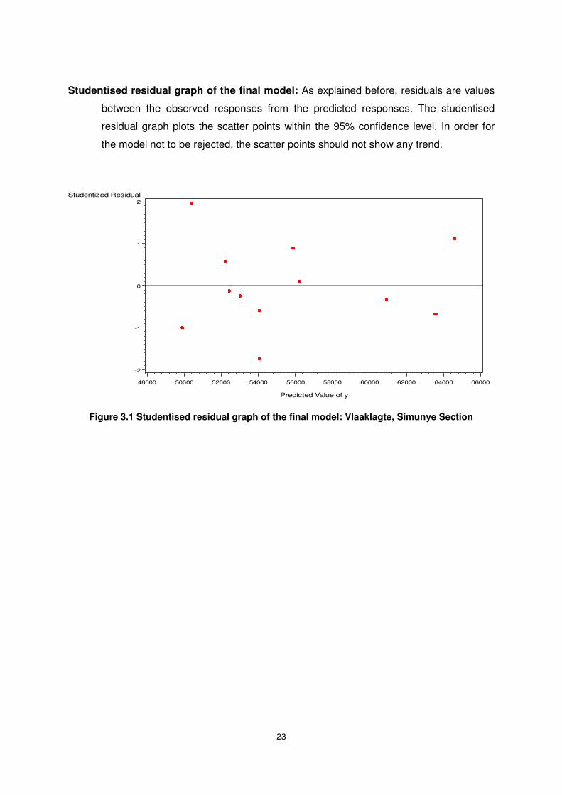
Studentised residual graph of the final model: As explained before, residuals are values

between the observed responses from the predicted responses. The studentised

residual graph plots the scatter points within the 95% confidence level. In order for

the model not to be rejected, the scatter points should not show any trend.

Figure 3.1 Studentised residual graph of the final model: Vlaaklagte, Simunye Section

Studentized Residual

-2

-1

0

1

2

Predicted Value of y

48000 50000 52000 54000 56000 58000 60000 62000 64000 66000

Studentized residual of the final model

24

Part IV

Computational Results

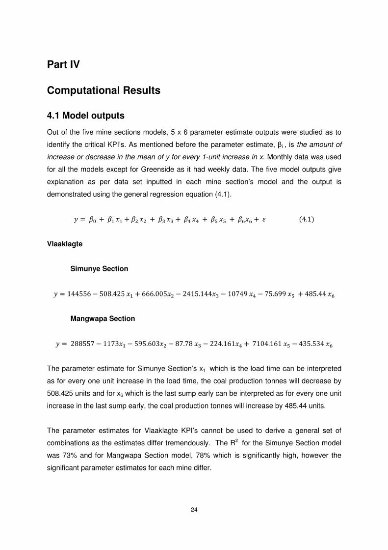
4.1 Model outputs

Out of the five mine sections models, 5 x 6 parameter estimate outputs were studied as to

identify the critical KPI’s. As mentioned before the parameter estimate, �i , is the amount of

increase or decrease in the mean of y for every 1-unit increase in x. Monthly data was used

for all the models except for Greenside as it had weekly data. The five model outputs give

explanation as per data set inputted in each mine section’s model and the output is

demonstrated using the general regression equation (4.1).

) �/N� (�/1�O1 ( /A�OA �( �/P�OP (�/Q�OQ �( �/R�OR �( �/HOH ( �5��6F89:

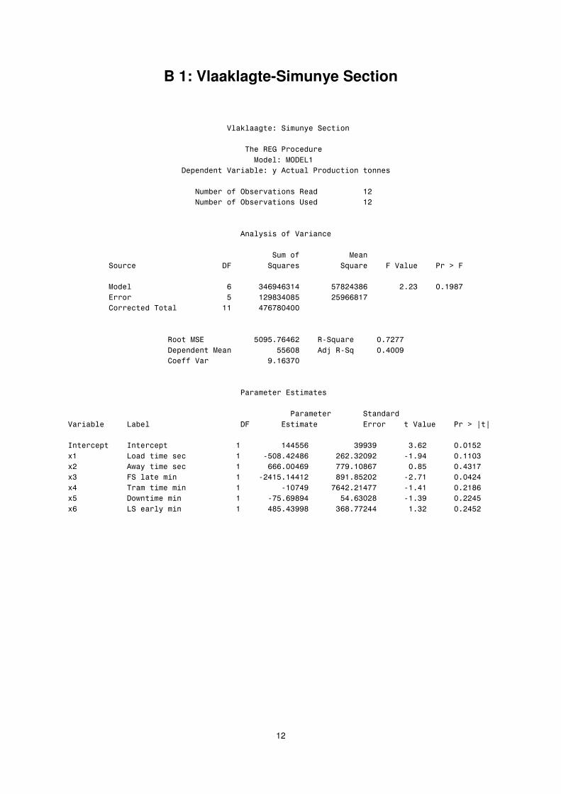
Vlaaklagte

Simunye Section

) 9FFGG% � G&S8F7G�O1 ( %%%8&&GOA � 7F9G89FFOP � 9&TFU�OQ � TG8%UU�OR �( FSG8FF�OH

Mangwapa Section

) �7SSGGT� 99T$O1 � GUG8%&$OA � ST8TS�OP � 77F89%9OQ ( �T9&F89%9�OR � F$G8G$F�OH

The parameter estimate for Simunye Section’s x1 which is the load time can be interpreted

as for every one unit increase in the load time, the coal production tonnes will decrease by

508.425 units and for x6 which is the last sump early can be interpreted as for every one unit

increase in the last sump early, the coal production tonnes will increase by 485.44 units.

The parameter estimates for Vlaaklagte KPI’s cannot be used to derive a general set of

combinations as the estimates differ tremendously. The R2 for the Simunye Section model

was 73% and for Mangwapa Section model, 78% which is significantly high, however the

significant parameter estimates for each mine differ.

25

Greenside

George Section

) �7$%T8%$S � 98G7%O1 � S8$$%OA �( �9F8S$TOP � 9%$8T7TOQ � 78F%7OR � %8%&&OH Vumangara Section

) �GUFS8FU7 ( �G8%9&O1 � $%8%FFOA � 9G877$OP � 77S8&GF�OQ � &8FGF�OR � $8S$%OH

The parameter estimates for Greenside differ slightly as compared to the Vlaaklagte

parameter estimates, however the R2 for both models were significantly low, 45% and 48%

for George and Vumagara respectively. If the model is not good enough, no KPI combination

can be derived from such a model.

New Denmard Central

Simunye Section

) TFG79 � 9&$8$�O1 � U8S$TOA � $9S8GF%OP � GSS%8SF�OQ ( F98G7S�OR � $%G89&T�OH

The R2 for the New Denmark section was 55% and the adjusted R2 has a negative value

which shows that the model contains terms that do not help in predicting the response.

All the parameter estimates where tested for significance and the significant parameter

estimates are as shown in the table 4.1.

Table 4.1: Significant parameter estimates

Section Name �1 �2 �3 �4 �5 �6

1 Greenside: Vumagara 1 1 1

2 NDC_Central :Simunye 1 1

3 Vlaaklagte: Simunye 1 1

4 Greenside: George 1

5 Vlaaklgate: Mangwapa 1

26

From the table, no parameter estimate(s) dominate the others. This can be due to the reality

that all the mines differ due to the following;

• shift patterns

• maintenance allowances

• pillar centers

• size of coal

• haulers

• daily mine’s section production targets etc.

From the five models, only three KPI’s dominated and this cannot be deemed legitimate as

the sample size of the models is minute. It should not be ignored that the five models did not

yield favorable outputs thus impeding further investigation due to the sample size being too

small &/other unknown factors.

4.2 Solution quality

Test for Model and parameter significance

As mentioned before, the t-test and F-test were used for checking model and parameter

significance. The p- value had to be below 20% were measurable changes were made, and

5% for all the other models using the rule of thumb.

27

Part IV

Recommendations

The model outputs did not show any trend that could be used to select a general KPI

combination. The data samples when tested using the normality test did not yield favorable

results thus suggesting the small sample size might be a problem. The parameter estimates

told a different story for each mine section even though some of the models were significant

and had more or less the same data points as the others.

However the model outputs gave ample information on the effect they have on the actual

production tonnes. As mentioned under future work, further regression analysis

methodologies can be carried out as to improve the solution integrity with the addition of a

bigger sample size.

5.1 Future work

One area that was not explored was the combination of some KPI’s by having a product of

two KPI’s as to check if the KPI’s combined will have an impact on the actual production

tonnes. What this would do is to increase the order of the regression model to two or three

degrees but the model would still be categorised as a linear model. The same goes for

having reciprocals or dividing some of the KPI’s.

It would be valuable to gather more data as to develop precise and bettered underground

mining KPI regression models that can be used for KPI combination selection and coal

production tonnes forecasting.

Data transformations can also aid in giving a better model fit and smaller prediction errors,

but also give a more reasonable bias structure as to how the KPI combination output would

fit a real life mining scenario. The type of transformation will depend on the theoretical

relationships between the response variable and the predictor variables.

One important lesson learnt is that one should not trust global measures of prediction

quality too much since they may be misleading. The values for all the models developed are

very reasonable, but the general interpretation of the individual output seemed bias.

28

Bibliography

[1] Berger, D.E. (2003). Introduction to Multiple Regression. Claremont Graduate

University. Pages1-6.

[2] Bise, C.J., and Albert, E.K. Comparison of model and simulation techniques for

production analysis in underground coal mines-document summary. Available online

from http://www.onemine.org/(Retrived 23 May 2009)

[3] Denkhaus, M. Eardley, M. Mufamadi, C. and Raphulu, R.(2007).Review of the

Current Approach to Measurement and Reporting of Continuous Miner Relocation

Time as a Key Performance Indicator. Presentation.

[4] Giltow, H.S., Oppenheim, A.J, and Levine, D.M.(2005). Quality management,3rd

edition. Singapore: McGraw Hill.

[5] Johnson, R.A,(2005).Probability and statistics for engineers.7TH edition. Pages 101-

146 and 226-281. United States of America: Prentice Hall.

[6] Khumalo, S. (2008). Determining the Suitability of the Current Functional Production

KPI’s at Greenside Colliery in Managing Production Section Downtime and To

Identify Critical Areas of Lost Time.

[7] Mendenhall, W, Sincich, T. A Second course in Statistics: Regression Analysis. 6th

edition, pages 90-741. New Jersey: Prentice-Hall.

[8] Montgomery, D.C, Peck, E.A, Vinig, G.G. Introduction to linear regression analysis.

Pages 169-217.

[9] Nass, P. (1999). Multivariate analysis methods. Available online from

www.eso.org/projects/esomidas/doc/user/.../node210.html (Retrieved on 19 August

2009)

29

[10] Nielsen, B. R, Stapelfeldt, H, Skibsted, L.F.(1997) Early Prediction of the Shelf-life

of Medium-heat Whole Milk Powders Using Stepwise Multiple Regression and

Principal Component Analysis. Royal Veterinary and University.

[11] Prinsloo, B, Steyn, P, and Ndiweni, A.(2006). Defining the standard Anglo Coal front

line performance measurements for Underground CM sections.

[12] Randall, D.T. An introduction to partial least square regression. SAS Institute Inc,

Cary, NC. Pages 1-4.

[13] Savage, L.S. (2003).Decision making with Insight, 1st edition, pages 17-50.Canada:

Thomson Brooks/Cole.

[14] Statsoft Website.(2009) Time Series Analysis. Available online from

www.statsoft.com/TEXTBOOK/sttimser.html.(Retrieved 10 October 2009)

[15] Tomerat, J.F, Harakal, C. (1996). Multiple Linear Regression Analysis of Blood

Pressure, Hypertrophy, Calcium and Cadmium in Hypertensive and Non-

hypertensive States. Temple University School of Medicine.

[16] Winston, L.W, Ventekataraman, M. Introduction to Mathematical Programming, 4th

edition, volume one of Operations Research, pages 49-111. California: Duxbury.

30

Addendum

Addendum A: Sections SAS models

A 1: Vlaaklagte: Mangwapa section

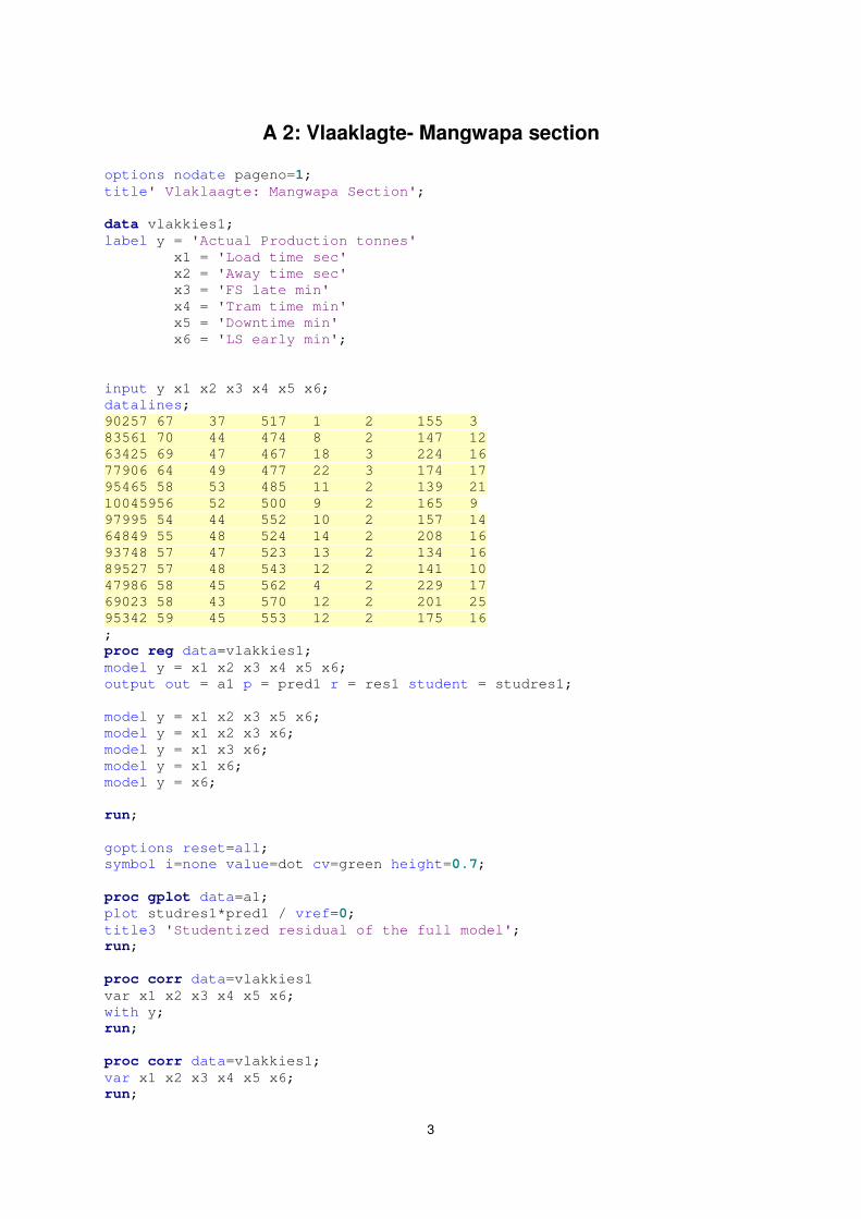
A 2: Vlaaklagte: Mangwapa Section

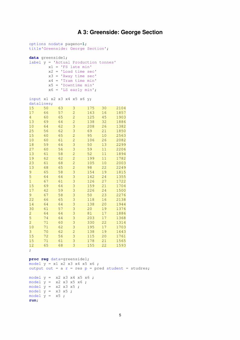
A 3: Greenside: George Section

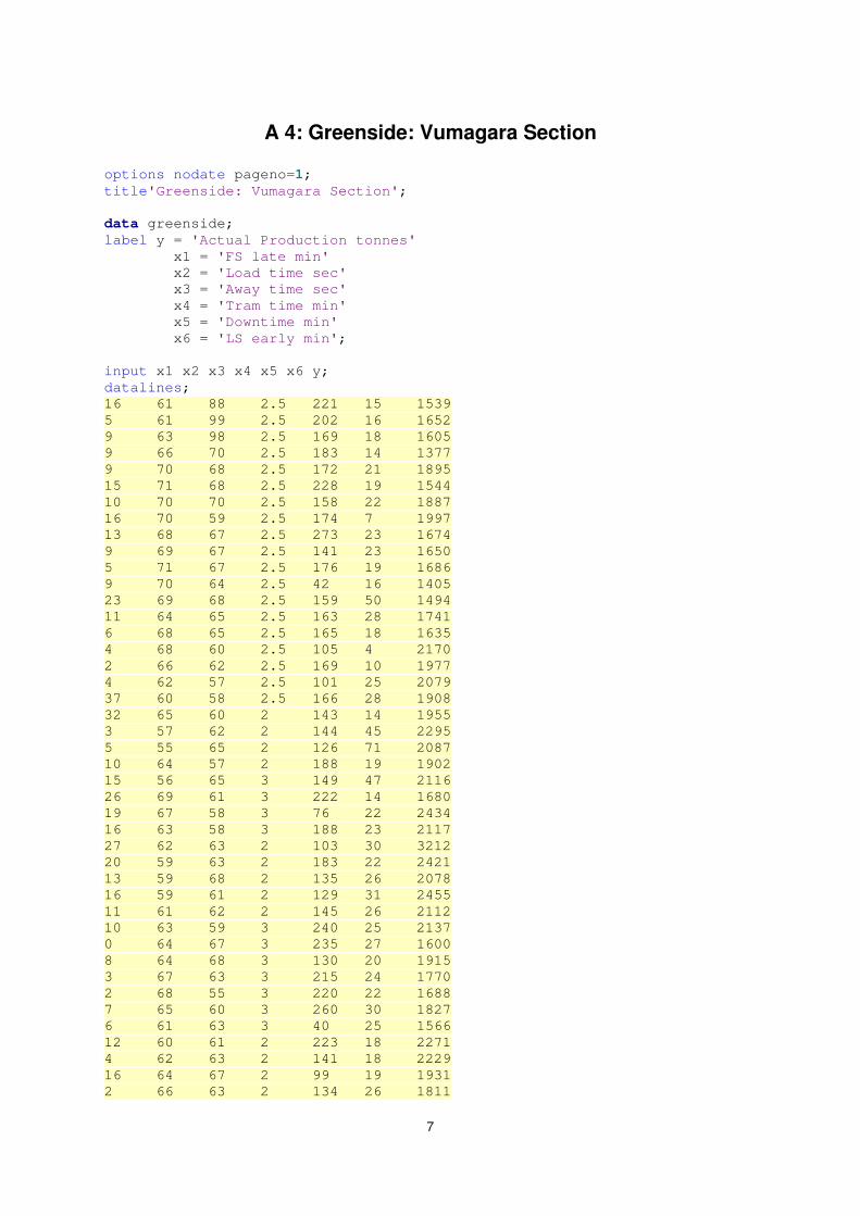
A 4: Greenside: Vumagara Section

A 5: New Denmark Colliery: Simunye Section

Addendum B: SAS sections model outputs

B 1: Vlaaklagte: Simunye Section

B 2: Vlaaklagte: Mangwapa Section

B 3: Greenside: George Section

B 4: Greenside: Vumagara Section

B 5: New Denmark Colliery: Simunye Section

Addendum A: Sections SAS models

1

A 1: Vlaaklagte: Simunye Section

options nodate pageno=1; title' Vlaklaagte: Simunye Section'; data vlakkies; label y = 'Actual Production tonnes' x1 = 'Load time sec' x2 = 'Away time sec' x3 = 'FS late min' x4 = 'Tram time min' x5 = 'Downtime min' x6 = 'LS early min'; input y x1 x2 x3 x4 x5 x6; datalines; 59457 63 72 22 3 304 13 54847 67 70 26 3 187 13 51350 67 74 25 4 155 16 60042 67 76 24 4 142 20 60898 66 71 20 4 143 8 51956 70 72 25 3 148 7 46085 67 70 25 3 203 5 45962 63 84 28 4 199 8 58854 67 71 27 3 167 6 52279 88 68 22 3 187 12 56704 66 66 24 3 201 19 68864 63 70 20 3 215 11 ; proc reg data=vlakkies; model y = x1 x2 x3 x4 x5 x6; output out = a1 p = pred1 r = res1 student = studres1; model y = x1 x3 x4 x5 x6; model y = x1 x3 x4 x5; model y = x1 x3 x4; model y = x1 x3 ; run; goptions reset=all; symbol i=none value=dot cv=green height=0.7; proc gplot data=a1; plot studres1*pred1 / vref=0; run; proc corr data=vlakkies; var x1 x2 x3 x4 x5 x6; with y; run; proc corr data=vlakkies;

2

var x1 x2 x3 x4 x5 x6; run; proc univariate data=vlakkies normal; var y x1 x2 x3 x4 x5 x6; histogram y x1 x2 x3 x4 x5 x6 /normal; run; **********Checking errors for normality for the fitted model*************; proc reg data=vlakkies; model y = x1 x3 ; output out=a p=pred r=res student=studres; run; proc print data=a; run; goptions reset=all; symbol i=none value=dot cv=red height=0.7; proc gplot data=a; plot studres*pred / vref=0; title3 'Studentized residual of the final model'; run;

3

A 2: Vlaaklagte- Mangwapa section options nodate pageno=1; title' Vlaklaagte: Mangwapa Section'; data vlakkies1; label y = 'Actual Production tonnes' x1 = 'Load time sec' x2 = 'Away time sec' x3 = 'FS late min' x4 = 'Tram time min' x5 = 'Downtime min' x6 = 'LS early min'; input y x1 x2 x3 x4 x5 x6; datalines; 90257 67 37 517 1 2 155 3 83561 70 44 474 8 2 147 12 63425 69 47 467 18 3 224 16 77906 64 49 477 22 3 174 17 95465 58 53 485 11 2 139 21 10045956 52 500 9 2 165 9 97995 54 44 552 10 2 157 14 64849 55 48 524 14 2 208 16 93748 57 47 523 13 2 134 16 89527 57 48 543 12 2 141 10 47986 58 45 562 4 2 229 17 69023 58 43 570 12 2 201 25 95342 59 45 553 12 2 175 16 ; proc reg data=vlakkies1; model y = x1 x2 x3 x4 x5 x6; output out = a1 p = pred1 r = res1 student = studres1; model y = x1 x2 x3 x5 x6; model y = x1 x2 x3 x6; model y = x1 x3 x6; model y = x1 x6; model y = x6; run; goptions reset=all; symbol i=none value=dot cv=green height=0.7; proc gplot data=a1; plot studres1*pred1 / vref=0; title3 'Studentized residual of the full model'; run; proc corr data=vlakkies1 var x1 x2 x3 x4 x5 x6; with y; run; proc corr data=vlakkies1; var x1 x2 x3 x4 x5 x6; run;

4

proc univariate data=vlakkies1 normal; var y x1 x2 x3 x4 x5 x6; histogram y x1 x2 x3 x4 x5 x6 /normal; run; **********Checking errors for normality for the fitted model*************; proc reg data=vlakkies1; model y = x6 ; output out=a p=pred r=res student=studres; run; proc print data=a; run; goptions reset=all; symbol i=none value=dot cv=red height=0.7; proc gplot data=a; plot studres*pred / vref=0; title3 'Studentized residual of the final model'; run;

5

A 3: Greenside: George Section options nodate pageno=1; title'Greenside: George Section'; data greenside1; label y = 'Actual Production tonnes' x1 = 'FS late min' x2 = 'Load time sec' x3 = 'Away time sec' x4 = 'Tram time min' x5 = 'Downtime min' x6 = 'LS early min'; input x1 x2 x3 x4 x5 x6 y; datalines; 15 50 63 3 175 30 2104 17 66 57 2 163 16 1857 4 60 65 2 125 45 1903 13 69 64 2 138 32 1886 10 64 62 3 208 26 1382 25 56 62 3 69 21 1850 15 60 65 2 95 10 2563 10 60 61 2 106 26 2082 18 59 64 3 50 13 2299 27 60 56 3 59 11 2206 13 61 58 2 52 11 1894 19 62 62 2 199 11 1782 23 61 68 2 105 10 2003 13 68 65 2 98 22 2249 9 65 58 3 154 19 1815 5 64 64 3 142 24 1355 1 67 61 3 126 27 1722 15 69 64 3 159 21 1704 17 42 59 3 226 24 1500 9 67 58 3 50 23 2276 22 66 65 3 118 16 2138 14 64 64 3 138 20 1944 30 61 57 3 20 19 1376 2 64 64 3 81 17 1886 5 74 64 3 203 17 1368 2 71 60 3 330 22 1314 10 71 62 3 195 17 1703 3 70 62 2 138 19 1643 15 72 56 3 115 20 1761 15 71 61 3 178 21 1565 12 65 68 3 155 22 1593 ; proc reg data=greenside1; model y = x1 x2 x3 x4 x5 x6 ; output out = a r = res p = pred student = studres; model y = x2 x3 x4 x5 x6 ; model y = x2 x3 x5 x6 ; model y = x2 x3 x5 ; model y = x3 x5 ; model y = x5 ; run;

6

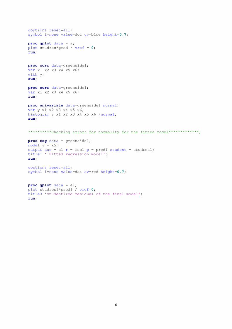
goptions reset=all; symbol i=none value=dot cv=blue height=0.7; proc gplot data = a; plot studres*pred / vref = 0; run; proc corr data=greenside1; var x1 x2 x3 x4 x5 x6; with y; run; proc corr data=greenside1; var x1 x2 x3 x4 x5 x6; run; proc univariate data=greenside1 normal; var y x1 x2 x3 x4 x5 x6; histogram y x1 x2 x3 x4 x5 x6 /normal; run; **********Checking errors for normality for the fitted model*************; proc reg data = greenside1; model y = x5; output out = a1 r = res1 p = pred1 student = studres1; title1 ' Fitted regression model'; run; goptions reset=all; symbol i=none value=dot cv=red height=0.7; proc gplot data = a1; plot studres1*pred1 / vref=0; title3 'Studentized residual of the final model'; run;

7

A 4: Greenside: Vumagara Section options nodate pageno=1; title'Greenside: Vumagara Section'; data greenside; label y = 'Actual Production tonnes' x1 = 'FS late min' x2 = 'Load time sec' x3 = 'Away time sec' x4 = 'Tram time min' x5 = 'Downtime min' x6 = 'LS early min'; input x1 x2 x3 x4 x5 x6 y; datalines; 16 61 88 2.5 221 15 1539 5 61 99 2.5 202 16 1652 9 63 98 2.5 169 18 1605 9 66 70 2.5 183 14 1377 9 70 68 2.5 172 21 1895 15 71 68 2.5 228 19 1544 10 70 70 2.5 158 22 1887 16 70 59 2.5 174 7 1997 13 68 67 2.5 273 23 1674 9 69 67 2.5 141 23 1650 5 71 67 2.5 176 19 1686 9 70 64 2.5 42 16 1405 23 69 68 2.5 159 50 1494 11 64 65 2.5 163 28 1741 6 68 65 2.5 165 18 1635 4 68 60 2.5 105 4 2170 2 66 62 2.5 169 10 1977 4 62 57 2.5 101 25 2079 37 60 58 2.5 166 28 1908 32 65 60 2 143 14 1955 3 57 62 2 144 45 2295 5 55 65 2 126 71 2087 10 64 57 2 188 19 1902 15 56 65 3 149 47 2116 26 69 61 3 222 14 1680 19 67 58 3 76 22 2434 16 63 58 3 188 23 2117 27 62 63 2 103 30 3212 20 59 63 2 183 22 2421 13 59 68 2 135 26 2078 16 59 61 2 129 31 2455 11 61 62 2 145 26 2112 10 63 59 3 240 25 2137 0 64 67 3 235 27 1600 8 64 68 3 130 20 1915 3 67 63 3 215 24 1770 2 68 55 3 220 22 1688 7 65 60 3 260 30 1827 6 61 63 3 40 25 1566 12 60 61 2 223 18 2271 4 62 63 2 141 18 2229 16 64 67 2 99 19 1931 2 66 63 2 134 26 1811

8

6 69 69 2 138 18 1844 6 66 64 2 183 23 2171 26 67 60 3 153 11 1898 3 64 57 2 173 19 2169 9 61 58 3 134 19 2012 15 64 60 2 214 20 2290 14 64 60 3 131 20 2068 ; proc reg data=greenside; model y = x1 x2 x3 x4 x5 x6 ; output out = a r = res p = pred student = studres; model y = x1 x2 x3 x4 x6 ; model y = x1 x2 x3 x4 ; model y = x2 x3 x4; run; goptions reset=all; symbol i=none value=dot cv=green height=0.7; proc gplot data = a; plot studres*pred / vref = 0; run; proc corr data=greenside; var x1 x2 x3 x4 x5 x6; with y; run; proc corr data=greenside; var x1 x2 x3 x4 x5 x6; run; proc univariate data=greenside normal; var y x1 x2 x3 x4 x5 x6; histogram y x1 x2 x3 x4 x5 x6 /normal; run; **********Checking errors for normality for the fitted model*************; proc reg data = greenside; model y = x2 x3 x4; output out = a1 r = res1 p = pred1 student = studres1; title1 ' Fitted regression model'; run; goptions reset=all; symbol i=none value=dot cv=red height=0.7; proc gplot data = a1; plot studres1*pred1 / vref=0; title3 'Studentized residual of the final model'; run;

9

A 5: New Denmark Colliery - Simunye Section options nodate pageno=1; title' NDC_Central: Simunye Section'; data ndc; label y = 'Actual Production tonnes' x1 = 'Load time sec' x2 = 'Away time sec' x3 = 'FS late min' x4 = 'Tram time min' x5 = 'Downtime min' x6 = 'LS early min'; input y x1 x2 x3 x4 x5 x6; datalines; 25628 96 90 26 5 267 26 25873 93 89 24 6 222 21 24785 88 95 13 7 236 8 24747 111 75 8 7 215 8 26208 114 76 21 5 232 24 28506 113 81 26 4 214 21 27930 115 79 21 6 260 9 22736 138 93 15 7 243 4 20597 116 85 14 6 159 5 36238 113 84 15 5 200 6 35034 113 84 18 5 173 13 ; proc reg data=ndc; model y = x1 x2 x3 x4 x5 x6; output out = a r = res p = pred student = studres; model y = x1 x3 x4 x5 x6; model y = x1 x4 x5 x6 ; model y = x1 x4 x6; model y = x4 x6 ; run; goptions reset=all; symbol i=none value=dot cv=green height=0.7; proc gplot data = a; plot studres*pred / vref = 0; run; proc corr data=ndc; var x1 x2 x3 x4 x5 x6; with y; run; proc corr data=ndc; var x1 x2 x3 x4 x5 x6; run;

10

proc univariate data=ndc normal; var y x1 x2 x3 x4 x5 x6; histogram y x1 x2 x3 x4 x5 x6 /normal; run; **********Checking errors for normality for the fitted model*************; proc reg data=ndc; model y = x4 x6; output out = a1 p = pred1 r = res1 student = studres1; run; proc print data = a1; run; goptions reset=all; symbol i=none value=dot cv=red height=0.7; proc gplot data = a1; plot studres1*pred1 / vref=0; title3 'Studentized residual of the final model'; run;

11

Addendum B: SAS sections model outputs

*Only one model output is included under this section, the rest of the output models are saved in the attached disc

12

B 1: Vlaaklagte-Simunye Section

��

�

��

��

�� !�� "�

�

��# � ��$�� "��%��"��&�

��# � ��$�� "��%��"�'"��&�

�

�

��!��"�"��$��

�

�� $��

�� (��) ��"��) ��(�� *�(�

�

��+��,-+.-+,�-��/01&-,1+��&2&,��32�.10�

��/��&.1,-31/��&/.++1�0�

��4��-0+013-33�

�

�

��/3./20+-+&��5) ��320&00�

��//+31��!�6��5)��32-33.�

��4��$$��.2�+,03�

�

�

��"��"�

�

��

�� (��"�� *�7�7�

�

8��8��--//+��,..,.��,2+&��323�/&�

9��"��5/312-&-1+��&+&2,&3.&��5�2.-��32��3,�

9&��!:��"��+++233-+.��00.2�31+0��321/��32-,�0�

9,��(��5&-�/2�--�&��1.�21/&3&��5&20��323-&-�

9-��5�30-.��0+-&2&�-00��5�2-��32&�1+�

9/��:��50/2+.1.-��/-2+,3&1��5�2,.��32&&-/�

9+��-1/2-,..1��,+1200&--��2,&��32&-/&�

� �

13

��

��

�

��

��/�

�� !�� "�

�

��# � ��$�� "��%��"��&�

��# � ��$�� "��%��"�'"��&�

�

�

��!��"�"��$��

�

�� $��

�� (��) ��"��) ��(�� *�(�

�

��&��&+//,+,..��,&0+1�..��/2++��323&/0�

��.��&��&--33��&,-0�//+�

��4��-0+013-33�

�

�

��-1--20-/�+��5) ��32//+.�

��//+31��!�6��5)��32-/1/�

��4��$$��120�&&.�

�

�

��"��"�

�

��

�� (��"�� *�

7�7�

�

8��8��&&++3��&�1/��/2+��32333,�

9��"��5,,12./.,,��&&320003.��5�2/-��32�/.��

9,��(��5�1,/20.3,��/0+2.,33&��5,2�1��323��

�

�

��

��4��

�

��;�� "��

��+�� "��9��9&��9,��9-��9/��9+�

�

�

��"��"�

�

�� #��%�� 9��

�

��&��//+31��+/1-��++0&.1��-/.+&��+11+-�

��9��&��+021,,,,��+2+1//1��1�-233333��+,233333��11233333�

��9&��&��0&233333��-2/0&+/��1+-233333��++233333��1-233333�

��9,��&��&-233333��&2//1-��&11233333��&3233333��&1233333�

��9-��&��,2,,,,,��32-.&,0��-3233333��,233333��-233333�

��9/��&��102/1,,,��--2+.�0.��&&/��-&233333��,3-233333�

��9+��&��2/3333��-2.+,/3��,1233333��/233333��&3233333�

�

��

�

��'#8�!�8!��

�� <!�� "=�

�

��"�

14

�

��#��&�� ;��"��&�

��//+312�++0�� "��%��"��++0&.1�

��%��+/1,2/.��0��-,,-,+0&20�

��:��""��32&133,,&.��> ��"�"��32�/�&1.-1�

��'��,20/1-��3��4��-0+013-33�

��4��$$��21,.&/&,��.332/�.30�

�

�

��

� �

15

� � � � ��?�"��"��" ��"�

�

��

�

��//+312�0��%��+/1-�

��//00/2/3��-,,-,+0,�

��2��&&.3&�

��8��) ��13.0�

�

�

��"�"�$�� 3@3�

�

��"��5��"��5��55555�� 555555�

�

�� A"��&.2&/.-+��*�7�7��B2333��

��+��*@�7�7��32333/�

��,.��*@�77��32333/�

�

�

��"�"�$��#��

�

��"��55��"��555��55555�� 555555�

�

��5;��;��32./+0+-��B�;��320,+1�

��>��%5��%��32�&0/�,��*��*32�/33�

��4��5%��"�"��;5)��323,&3/0��*�;5)��*32&/33�

��!��"��5��!5)��32&--000��*�!5)��*32&/33�

�

��'#8�!�8!��

��(��#��"�� $��

�

��"�$��#��"��

�

�� "��

�

�� //+312�0�

��%��+/1,2/.��

�

�

��""5�$5(��"�"�$��#��"��

�

��"��5555��"��55555��555555�� 555555�

�

��>��%5��%��32�&0/�,�0��*��*32�/3�

��4��5%��"�"��;5)��323,&3/+..��*�;5)��*32&/3�

��!��"��5��!5)��32&--000-.��*�!5)��*32&/3�

�

�

��

��

�

��'#8�!�8!��

�� 9��<��"��=�

�

��"�

�

��#��&�� ;��"��&�

��+021,,,,,,�� "��%��"��1�-�

��%��+2+1//0.&,��--2+.+.+.0�

��:��""��&21+1+-1-��> ��"�"��.2�-/&1�/+�

��'��//031��4��-.�2+++++0�

��4��$$��.21//1.30+��2.&..+3-.�

16

�

�

��?�"��"��" ��"�

�

��

�

��+021,,,,��%��+2+1//1�

��+0233333��--2+.+.0�

��+0233333��&/233333�

��8��) ��&2/3333�

�

�

��

� �

17

� � � � ��"�"�$�� 3@3�

�

��"��5��"��5��55555�� 555555�

�

�� A"��,/2�-0/&��*�7�7��B2333��

��+��*@�7�7��32333/�

��,.��*@�77��32333/�

�

��

�

�

��"�"�$��#��

�

��"��55��"��555��55555�� 555555�

�

��5;��;��32+3�.-&��B�;��32333��

��>��%5��%��32,1&.,&��*��B323�33�

��4��5%��"�"��;5)��32,/&,/+��*�;5)��B3233/3�

��!��"��5��!5)��2.�1�&��*�!5)��B3233/3�

�

�

��

�

��'#8�!�8!��

��(��#��"�� $��9��

�

��"�$��#��"��

�

�� "��

�

�� +021,,,,�

��%��+2+1//0.�

�

�

��""5�$5(��"�"�$��#��"��

�

��"��5555��"��55555��555555�� 555555�

�

��>��%5��%��32,1&.,�/1��*��B323�3�

��4��5%��"�"��;5)��32,/&,//+-��*�;5)��B3233/�

��!��"��5��!5)��2.�1�&3,.��*�!5)��B3233/�

�

�

��

��

�

��'#8�!�8!��

�� 9&��<!:��"��=�

�

��"�

�

��#��&�� ;��"��&�

��0&�� "��%��"��1+-�

��%��-2/0&+-/.-��&32.3.3.3.�

��:��""��203-+/-0/��> ��"�"��-2��/./-+,�

��'��+&-,1��4��&,3�

��4��$$��+2,/31.0�-��2,&333.�1�

�

�

��?�"��"��" ��"�

�

��

18

�

��0&233333��%��-2/0&+/�

��0�233333��&32.3.3.�

��03233333��1233333�

��8��) ��,233333�

�

�

�

�

��

� �

19

� � � � ��"�"�$�� 3@3�

�

��"��5��"��5��55555�� 555555�

�

�� A"��/-2/-/31��*�7�7��B2333��

��+��*@�7�7��32333/�

��,.��*@�77��32333/�

�

�

��"�"�$��#��

�

��"��55��"��555��55555�� 555555�

�

��5;��;��321-+0&&��B�;��323,,/�

��>��%5��%��32&/��*��323,0+�

��4��5%��"�"��;5)��32�,31-0��*�;5)��323,1,�

��!��"��5��!5)��320+-,-/��*�!5)��323,/��

�

�

��

��

�

��'#8�!�8!��

��(��#��"�� $��9&�

�

��"�$��#��"��

�

�� "��

�

�� 0&�

��%��-2/0&+-+�

�

�

��""5�$5(��"�"�$��#��"��

�

��"��5555��"��55555��555555�� 555555�

�

��>��%5��%��32&/333333��*��323,1�

��4��5%��"�"��;5)��32�,31-0�3��*�;5)��323,1�

��!��"��5��!5)��320+-,--0/��*�!5)��323,/�

�

�

��

�

��'#8�!�8!��

�� 9,��<(��=�

�

��"�

�

��#��&�� ;��"��&�

��&-�� "��%��"��&11�

��%��&2//1-31+��+2/-/-/-//�

��:��""��532&0,+30+��> ��"�"��5320&,�-1��

��'��+.1-��4��0&�

��4��$$��32++33,/1��320,1/-1./�

�

�

��

�

�

��?�"��"��" ��"�

�

20

��

�

��&-233333��%��&2//1-��

��&-2/3333��+2/-/-/�

��&/233333��1233333�

��8��) ��,2/3333�

�

�

��

� �

21

� � � � � ��"�"�$�� 3@3�

�

��"��5��"��5��55555�� 555555�

�

�� A"��,&2-.+�/��*�7�7��B2333��

��+��*@�7�7��32333/�

��,.��*@�77��32333/�

�

�

��"�"�$��#��

�

��"��55��"��555��55555�� 555555�

�

��5;��;��32.--�0/��B�;��32//-3�

��>��%5��%��32�++++0��*��*32�/33�

��4��5%��"�"��;5)��323/�30,��*�;5)��*32&/33�

��!��"��5��!5)��32,3.+&��*�!5)��*32&/33�

�

�

��

�

��'#8�!�8!��

��(��#��"�� $��9,�

�

��"�$��#��"��

�

�� "��

�

�� &-�

��%��&2//1-3.�

�

�

��""5�$5(��"�"�$��#��"��

�

��"��5555��"��55555��555555�� 555555�

�

��>��%5��%��32�++++++0��*��*32�/3�

��4��5%��"�"��;5)��323/�30,,1��*�;5)��*32&/3�

��!��"��5��!5)��32,3.+�./1��*�!5)��*32&/3�

�

�

��

��

�

��

� �

22

��'#8�!�8!��

�� 9-��<��=�

�

��"�

�

��#��&�� ;��"��&�

��,2,,,,,,,,�� "��%��"��-3�

��%��32-.&,+/.+��32&-&-&-&-�

��:��""��321�&-3,1-��> ��"�"��5�2+/�

��'��,+��4��&2+++++++0�

��4��$$��-2003.01.��32�-&�,,1��

�

�

��?�"��"��" ��"�

�

��

�

��,2,,,,,,��%��32-.&,0�

��,2333333��32&-&-&�

��,2333333��233333�

��8��) ��233333�

�

�

��"�"�$�� 3@3�

�

��"��5��"��5��55555�� 555555�

�

�� A"��&,2-/&31��*�7�7��B2333��

��+��*@�7�7��32333/�

��,.��*@�77��32333/�

�

�

��"�"�$��#��

�

��"��55��"��555��55555�� 555555�

�

��5;��;��32+313.��B�;��32333��

��>��%5��%��32-�0-+/��*��B323�33�

��4��5%��"�"��;5)��32-�-0./��*�;5)��B3233/3�

��!��"��5��!5)��&2,&,/.��*�!5)��B3233/3�

�

�

��

��

�

��

� �

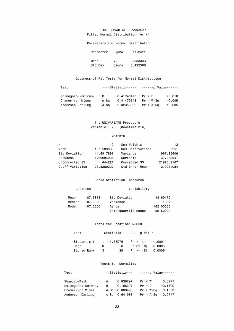
23

��'#8�!�8!��

��(��#��"�� $��9-�

�

��"�$��#��"��

�

�� "��

�

�� ,2,,,,,,�

��%��32-.&,++�

�

�

��""5�$5(��"�"�$��#��"��

�

��"��5555��"��55555��555555�� 555555�

�

��>��%5��%��32-�0-+-03��*��B323�3�

��4��5%��"�"��;5)��32-�-0./-1��*�;5)��B3233/�

��!��"��5��!5)��&2,&,/1..1��*�!5)��B3233/�

��

��

��

��'#8�!�8!��

�� 9/��<��:��=�

�

��"�

�

��#��&�� ;��"��&�

��102/1,,,,�� "��%��"��&&/��

��%��--2+.�01.+��..02,/+3+�

��:��""��2+3.1-.,+��> ��"�"��,20&,,/-��

��'��---&&��4��&�.032.�+0�

��4��$$��&,21&/3,&&��&2.3�-31-�

�

�

��?�"��"��" ��"�

�

��

�

��102/1,,��%��--2+.�0.�

��1023333��..0�

��1023333��+&233333�

��8��) ��/32/3333�

�

�

��"�"�$�� 3@3�

�

��"��5��"��5��55555�� 555555�

�

�� A"��-2/,.0+��*�7�7��B2333��

��+��*@�7�7��32333/�

��,.��*@�77��32333/�

�

�

��"�"�$��#��

�

��"��55��"��555��55555�� 555555�

�

��5;��;��321,.&.0��B�;��323&0��

��>��%5��%��32�.1,.0��*��*32�/33�

��4��5%��"�"��;5)��3231+-.+��*�;5)��32�//,�

��!��"��5��!5)��32+-�.+1��*�!5)��3230-0�

��

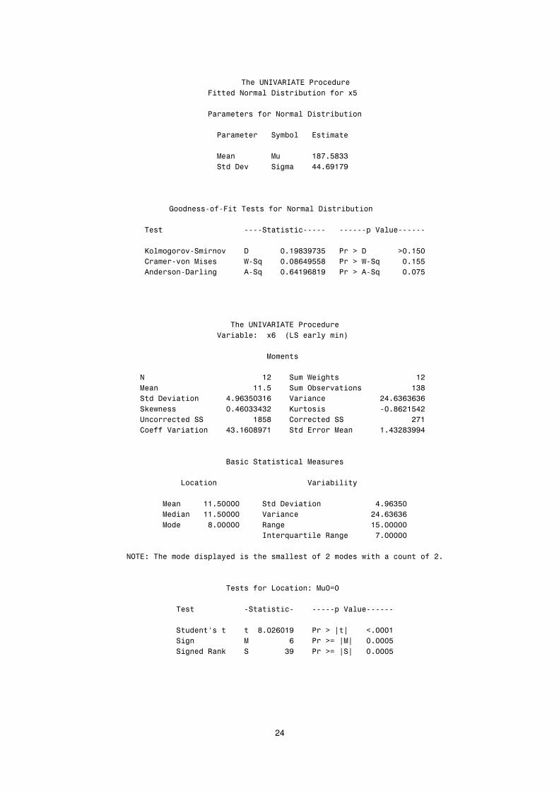
24

�

�� '#8�!�8!��

��(��#��"�� $��9/�

�

��"�$��#��"��

�

�� "��

�

�� 102/1,,�

��%��--2+.�0.�

�

�

��

� � � ��""5�$5(��"�"�$��#��"��

�

��"��5555��"��55555��555555�� 555555�

�

��>��%5��%��32�.1,.0,/��*��*32�/3�

��4��5%��"�"��;5)��3231+-.//1��*�;5)��32�//�

��!��"��5��!5)��32+-�.+1�.��*�!5)��3230/�

�

�

��

�

��'#8�!�8!��

�� 9+��<��=�

�

��"�

�

��#��&�� ;��"��&�

��2/�� "��%��"��,1�

��%��-2.+,/3,�+��&-2+,+,+,+�

��:��""��32-+3,,-,&��> ��"�"��5321+&�/-&�

��'��1/1��4��&0��

��4��$$��-,2�+31.0��2-,&1,..-�

�

�

��?�"��"��" ��"�

�

��

�

��2/3333��%��-2.+,/3�

��2/3333��&-2+,+,+�

��1233333��/233333�

��8��) ��0233333�

�

��#��"��"��"��"��$�&��"�:�� $�&2�

�

�

��"�"�$�� 3@3�

�

��"��5��"��5��55555�� 555555�

�

�� A"��123&+3�.��*�7�7��B2333��

��+��*@�7�7��32333/�

��,.��*@�77��32333/�

�

�

��

� �

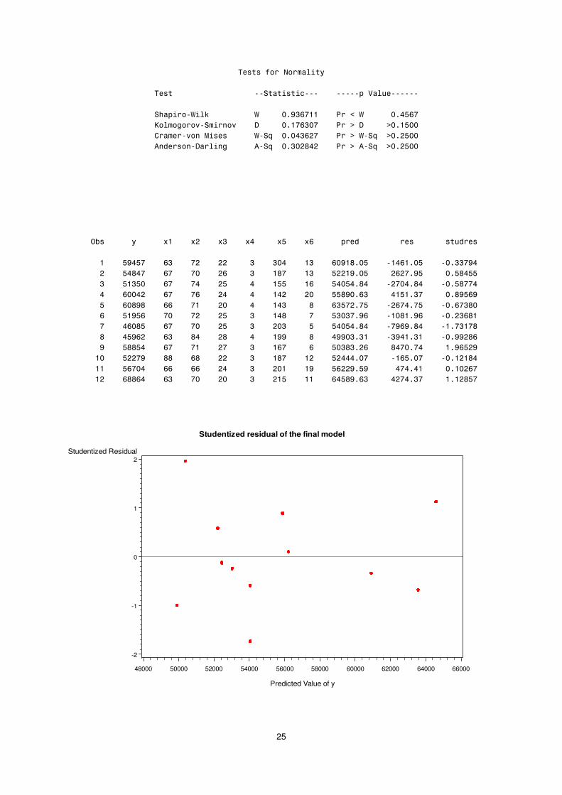
25

��"�"�$��#��

�

��"��55��"��555��55555�� 555555�

�

��5;��;��32.,+0��B�;��32-/+0�

��>��%5��%��32�0+,30��*��*32�/33�

��4��5%��"�"��;5)��323-,+&0��*�;5)��*32&/33�

��!��"��5��!5)��32,3&1-&��*�!5)��*32&/33�

�

�

�

��

��

�

��

�

�� "��9��9&��9,��9-��9/��9+��"��"� ��"�

�

��/.-/0��+,��0&��&&��,��,3-��,��+3.�123/��5�-+�23/��532,,0.-�

��&��/-1-0��+0��03��&+��,��10��,��/&&�.23/��&+&02./��32/1-//�

��,��/�,/3��+0��0-��&/��-��//��+��/-3/-21-��5&03-21-��532/100-�

��-��+33-&��+0��0+��&-��-��-&��&3��//1.32+,��-�/�2,0��321./+.�

��/��+31.1��++��0��&3��-��-,��1��+,/0&20/��5&+0-20/��532+0,13�

��+��/�./+��03��0&��&/��,��-1��0��/,3,02.+��5�31�2.+��532&,+1��

��0��-+31/��+0��03��&/��,��&3,��/��/-3/-21-��50.+.21-��5�20,�01�

��1��-/.+&��+,��1-��&1��-��..��1��-..3,2,��5,.-�2,��532..&1+�

��.��/11/-��+0��0��&0��,��+0��+��/3,1,2&+��1-0320-��2.+/&.�

��3��/&&0.��11��+1��&&��,��10��&��/&---230��5�+/230��532�&�1-�

��/+03-��++��++��&-��,��&3��.��/+&&.2/.��-0-2-��32�3&+0�

��&��+11+-��+,��03��&3��,��&�/��+-/1.2+,��-&0-2,0��2�&1/0�

�

�

Studentized Residual

-2

-1

0

1

2

Predicted Value of y

48000 50000 52000 54000 56000 58000 60000 62000 64000 66000

Studentized residual of the final model

identification of critical key performance indicators … · identification of critical key...

Documents