identification of anomalous movements of thunderstorms...
TRANSCRIPT
____________ * Electronic address: [email protected]
Identification of anomalous movements of thunderstorms using radar and satellite data
Author: Anna del Moral Méndez Supervisors: Mª del Carme Llasat Botija, [email protected]
Tomeu Rigo Ribas, [email protected] Facultat de Física, Universitat de Barcelona, Diagonal 645, 08028 Barcelona, Spain*.
Abstract: One of the most adverse weather phenomena in Catalonia are thunderstorms producing severe weather
phenomenon like heavy rainfalls, hail storms, or tornadoes. Sometimes, these thunderstorms seem to have marked paths although in some cases these trajectories vary sharply, changing completely the movement directions that have previously followed, either breaking into several cells, or joining into a bigger one. In order to identify the main features of the developing process of thunderstorms and the anomalous movements that these may in some cases follow, this paper presents a methodology that follows 3 main steps; previous classification of the events, cell identification, and finally, tracking of the cells identified. The methodology combines radar and satellite images.
I. INTRODUCTION
Thunderstorms produce most of the severe weather phenomena in the western Mediterranean region (strong winds, heavy rains, lightning, hail and tornadoes). In the case of Catalonia they occur mainly in summer and autumn seasons (Llasat, 2001; Rigo et al., 2008), and in some occasions they may produce floods and/or significant material damages with partial or complete destruction of some infrastructure or buildings, important losses on agriculture, farming, and human lives (Llasat et al., 2005).
We can highlight several cases that affected Catalonia in just the last fifteen years. This is the case of the tornado event in Ivars d'Urgell the 21st March 2012, causing damages on roofs and covers of buildings and farm warehouses (Bech et al., 2015). Among other tornado episodes, the outbreak in Barcelona the 7th September 2005 will be remembered by having affected a densely populated and urbanized area and, specially, the Barcelona International Airport (Bech et al., 2007). On the other hand, an important flood event occurred in Montserrat the 10th June 2000, causing the partial destruction of the Montserrat Monastery where about 500 people had to be evacuated, the material damage was estimated around 65 000 000 € and there were five fatalities (Llasat et al., 2003). Another relevant flood event took place in Vall d'Aran the 18th June 2013 that affected roads, electricity pylons and wastewater treatment plants and other infrastructures (IGC, 2013). Finally, we cannot forget the hail storm that occurred in Pla d'Urgell the 17th September 2007, affecting 889 ha of fruit tree fields (Farnell et al., 2009).
II. BACKGROUND
A. Thunderstorm lifecycle
A thunderstorm is the result of a deep convection region with strong updrafts (larger than 10 m/s), covering most of the troposphere. The horizontal section usually spans between 10 and 100 km² (Martín et al., 2007). The thunderstorm can last from 20 minutes to several hours, and three stages are identified during life cycle. The main differences between stages are the direction of vertical flows and the effects on the surface. Firstly, the development stage
presents a predominant updraft, making the small particles included into the cloud to grow. The growth lasts until the particles have the weight needed to cancel the upward force, coinciding with the beginning of the mature phase, and the precipitation of the particles. Precipitation creates a downdraft that counteracts the updraft, triggering an evaporation process and producing a cooling of the air temperature that accelerates the downward movement. Once the downdraft reaches the surface, a relatively small mass of cold air and a gust front, are generated. Finally, in the dissipating stage the downdraft predominates, which concludes when these disappears (Martín et al., 2007; Doswell, 2001 and Wilhemson, 1974).
B. Thunderstorm identification and classification
Three main types of thunderstorms can be identified using radar, based on the internal dynamics and organization (the height of the first echo sign in the radar, and how it evolves horizontally and vertically): simple, multicellular, and supercellular (Doswell et al., 1996). However, some more accurate classifications can be found in the bibliography. For instance, Rigo and Llasat (2004) took into account other previous characterizations, and developed a new classification, based on the type of precipitation, the size of each part of the rainfall structure (stratiform and convective), and the duration of the system. This classification is based on the identification of precipitation structures for each image, using a 2-D algorithm method. Following this last one, precipitation structures can be classified as:
§ Mesoscale Convective System: it is a type of
multicell (see below) in which the major axis has a length equal or larger than 100 km during 3 h or more. It is also required that at least of a 30% of the area can be associated with convective rainfall. § Multicell: presents some grouped convective areas,
but does not meet the conditions of time and size for being a Mesoscale Convective System. § Isolated convection: small scale areas with
independent and separate convective areas (the stratiform area is less than 30% during most of the life cycle).
Màster de Meteorologia 2 Universitat de Barcelona, Curs 2014-2015
§ Convection embedded in stratiform rainfall: a
stratiform region with some convective nucleus (with an area fewer than the 30% of the total echo region). § Stratiform: the convective rainfall does not exceed
3% of the total area. Other ways to identify and classify convection are based
on rain gauge data, like intensity or accumulation of precipitation. An example of this methodology can be found in Llasat (2001) that classifies an episode as convective if the intensity of 1 min-precipitation exceeds the value of 50mm/h, allowing to define the β parameter, related with the magnitude of the convective character of the event. Furthermore, following the recommendation made in the framework of the MEDEX project (a part of the WMO-World Weather Research Programme: (http://medex.aemet.uib.es) (Jansa et al., 2014), we can consider an event to be a High Precipitation Event if the accumulated precipitation exceeds the value of 60 mm/24 h. However, in this research, a reduced threshold has been used based on the interest in identifying very intense episodes.
Although rain gauges measure rainfall accurately, this information is localised and needs interpolation to obtain rainfall maps of our region of interest. Furthermore, high variability of convective precipitation makes the interpolations unrealistic in most of cases (Goodrich et al., 1995; Tapia et al., 1998). For that reason, weather radar combined with rain gauge information is the best option when spatial variability gains importance, like in regions where convection is usual and important (Velasco-Forero et al., 2009). Merging radar and rain gauge data, it is possible to obtain accurate methodologies that provide more information about convection. For example, Rigo and Llasat (2007) identify convective cells from a 2-D and a 3-D algorithm requiring that a convective cell must present reflectivity echoes grater than 43 dBZ (2-D algorithm), a high variability, a large gradient of reflectivity values between adjacent pixels and, finally, searching for the reflectivity core in each radar volume (3-D algorithm). Taking a step forward, Barnolas et al. (2010) suggest that, once the previous identification is done, those convective cells with an area greater than 32 km2 are geometrically characterized, approaching their shape to an ellipse, as proposed in Northop (1998) and Feral et al. (2000). Finally, it is possible to make a statistical description of the convection in a region of study, by means of the geometrical characterisation and the convective indicators computed from the rain gauge data.
C. Thunderstorm nowcasting
Nowadays, there are different ways to characterize and nowcast convective cells. Furthermore, it is possible to get some indicators that can provide a forecast of severe phenomena associated to them. However, the forecasting is still a challenge in some complex cases, which are those that cause the greatest problems to the society, and that are influenced by factors that have been studied only in isolated events. For instance, the Meteorological Service of Catalonia issues hazard warnings for high intensities precipitation
events only about fifteen minutes before the episode. However no warnings for other severe weather phenomena like downbursts, tornadoes or hail storms are issued
The cell motion, often erratic, constitutes one of the phenomena that complicates most the nowcasting of convective cells. Theoretically, studying the motion associated to the convective echoes referred to a certain reflectivity threshold, it is possible to obtain the displacement of the thunderstorm, which has two main factors: the translation and the propagation. The last one is divided in forced propagation and auto-propagation. Most of thunderstorms are just a system whose motion is controlled by the mean wind at the layer where they are (translation predominance). This occurs when the winds are very intense in deeper atmospheric layers and hence motion is easy to predict. However, there are some convective structures that move to the opposite direction to the main advective flow does (propagation predominance), when the tropospheric winds at medium and high levels are weaker, and therefore, it is more difficult to predict (Martín et al., 2007; Parker and Johnson, 2000). Furthermore, some convective structures may be influenced by the orography, the cold pool of the thunderstorm, the shear interactions, or the interaction with close cells, what may produce phenomena like merging, splitting, and stationary cells, among others anomalous motion.
Taking the mean wind as reference, the motion of a convective system can be classified by the following labels: forward moving systems, retrograde systems, quasi-steady systems and “convective trains” (Doswell, 2001). In the first case, the cells regenerate in a flank downstream of the main flow, with only few cells generating intense and short lasting precipitation. The second class has cells forming in a flank upstream of the main flow. Sometimes, these may seem to be stationary or moving counter-current, generating intense and long lasted precipitation and floods. Finally, quasy-steady systems are those whose propagation and translation movements cancel each other and, therefore, generate structures that remain fixed at the same region. Sometimes a place is affected by several cells that go through it in a stage of elevated rainfall efficiency (known as convective train effect). These convective systems produce the highest accumulations of precipitation at surface. Anomalous motion is detectable with the nowcasting algorithm of the SMC (Rigo and Llasat, 2002), based on the identifications of radar structures, the tracking of these and the extrapolation of the centroid position up to one hour. We can detect when a cell has anomalous motion because the thunderstorm core path forecasted and the real one are different, indicating that the speed and/or propagation direction differ. There are also other nowcasting algorithms similar to this, like the Thunderstorm Interactive Forecast System (TIFS), developed by the Australian Bureau of Meteorology in order to interactively produce severe weather warnings and other forecasts from thunderstorm tracks derived from radar data (Bally, 2004).
Other methodologies developed used to forecast a cell motion (especially supercells, which are the ones associated with anomalous motion and most severe weather) can be found in Bunkers et al. (2000), and Fujita and Grandoso (1968). The first one is based on the vertical wind shear profiles (hodograph). It makes the assumption that supercell
Màster de Meteorologia 3 Universitat de Barcelona, Curs 2014-2015
motion is the vector sum of two components: the advection represented by the mean wind vector and the shear-induced propagation to the direction of the wind shear vector towards which the storm is moving. Therefore, the position of the hodograph in some specific quadrants and its typology allow us to establish whether the cell is moving faster than the
mean wind and which its rotation direction would be. The second methodology is based on the different orientations that a thunderstorm anvil seen from satellite can have depending on its movement. It identifies the supercell motions by the anvil.
orientation, making the assumption that this does not depend just on the mean anvil-level winds, but also on the storm’s own motion, so that the combination of both gives the differences in between the anvil orientations, identified by using geostationary satellite images. Convection can be studied from MSG satellite imagery IR and VIS channels radiances. The EUMETSAT Convection Working Group (www.essl.org/cwg/) summarises the tools and algorithms to identify and nowcast convection by four categories, corresponding to a particular phase in the development of convective systems: the pre-convective environment, the convective initiation, the mature convective system and, finally, the monitoring and nowcasting of the resulting storms. In the first category it can be found the Global Instability index (GII), a MSG meteorological product that describes the instability of the clear atmosphere by a number of air-mass parameters. This product includes two instability indices (Lifted Index and K-Index), plus the Total Precipitable Water Content (TPW), that allows indicate the potential for convection, few hours prior to the onset of this (Koenig and de Coning, 2009). In the second category, it can be found a product called Convective Initiation (CI), which identifies cumulus-type clouds and uses temporal evolution of the related MSG observations, with the purpose of identifying rapidly growing cumulus as candidates to becoming potentially strong convective storms in the next hour. In this product, VIS and IR data are processed to obtain eight predictors for describing the character, growth and evolution of convective clouds (Mecikalski and Bedka, 2006). These predictors include IR cloud-top brightness temperature, which has been used in our research as an indicator of convection. Besides this, it also exist a product called RDT (Rapid Development Thunderstorm) developed by Météo-France within the framework of EUMETSAT SAF in support to Nowcasting, that provides cloud information in order to forecast future movement of convective cells (Morel et al. 2002). The RDT product uses stationary satellite data to detect rapid development of convective cells. However, this algorithm is just able to identify, monitor and track intensive convective system clouds, much larger than simple cells. In the third category, it can be found different products related to the mature phase of a thunderstorm. These include products to obtain information about the precipitation formation process, an algorithm to assess the presence of thunderstorms and their intensity, and, furthermore, the one used in this research: a product to obtain the Overshooting Top of a cloud, which gives the cumulonimbus anvil information, representing the intrusion of an updraft through its equilibrium level, that it is widely explained in the methodology section (Bedka, 2010). Finally, in the fourth category it can be found different tools to visualize and analyze data from MSG, like the IR Cold Cloud Tops, used in this research, that enables to identify better convection by colouring the cloud tops between 200 and 240 K from a MSG IR10.8 (channel 9) image using a fixed coloured scheme from blue to turquoise to yellow and red.
The main goal of this paper is the development of a technique for the identification and tracking of convective cells by means of volumetric radar data, in order to identify and forecast their anomalous motion. In addition, it has been introduced satellite product images as a completely new routine in the SMC nowcasting algorithm. This has shown promising results for improving the identification and nowcasting of the convective cells in the most complicated situations. The presented methodology is applicable to the region of Catalonia, and is capable of demonstrating that when additional data sources as satellite data or wind profiles from radiosounding are ingested the short-term forecasting of severe weather is more reliable.
The work presented is structured as follows: first, Section 3 describes the region and dataset used in the study; Section 4 presents the methodology to identify and track convective cells based on radar and satellite data; Section 5 summarizes the results obtained in this research, presents study case examples and the finally the conclusions synthesize the work and propose possible further studies.
III. STUDY REGION AND DATA
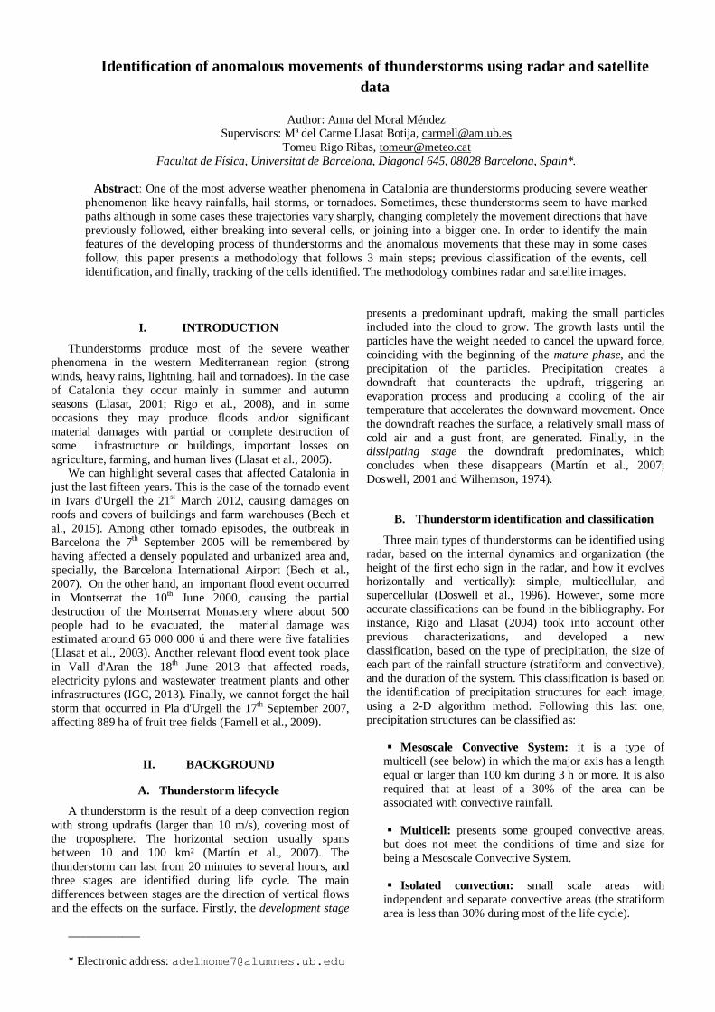
Catalonia is a region at the northeast of the Iberian Peninsula covering an area of near 35000 km2 (Fig.1). The location of the region, near the Mediterranean Sea, and its complex orography (with the Pyrenees at the north exceeding the 3000 m of altitude) are conditions that favour the generation, triggering and development of all kind of thunderstorms. These usually bring on the generation of heavy rainfall events, producing flash-floods or tornadoes on the steep coastal basins, mainly during late summer and autumn (Barnolas and Llasat, 2007; Gayà et al., 2011). Moreover during these seasons, the large Central Depression and Pla d'Urgell (Fig.1), are often the scenario for the development of severe thunderstorms associated with associated important damage causing phenomena like tornadoes, downburst or hail storms. For this study, volumetric radar data from the Meteorological Radar Network of the SMC (Fig. 2) has been used hence forward the XRAD Xarxa de Radars Meteorològics. The XRAD is composed by four Doppler radars operating in C band; Puig Bernat (Vallirana, near Barcelona) installed in 1996 by the University of Barcelona, Puig d’Arques, installed in 2002, Creu del Vent, installed in 2003, which are described in Bech et al. (2004), and La Miranda, installed in 2008, Their specific location is listed in Table I.
Table I: Details of the radar locations.
Code Location Latitude Longitude Altitude PBE Puig Bernat 41.37º N 1.88º E 610 m PDA Puig d’Arques 41.89º N 2.99º E 535 m CDV Creu del Vent 41.60º N 1.40 º E 825 m LMI La Miranda 41.09º N 0.86º E 925 m
Màster de Meteorologia 4 Universitat de Barcelona, Curs 2014-2015
Figure 1: Region of study .Catalonia with its main orographic features.
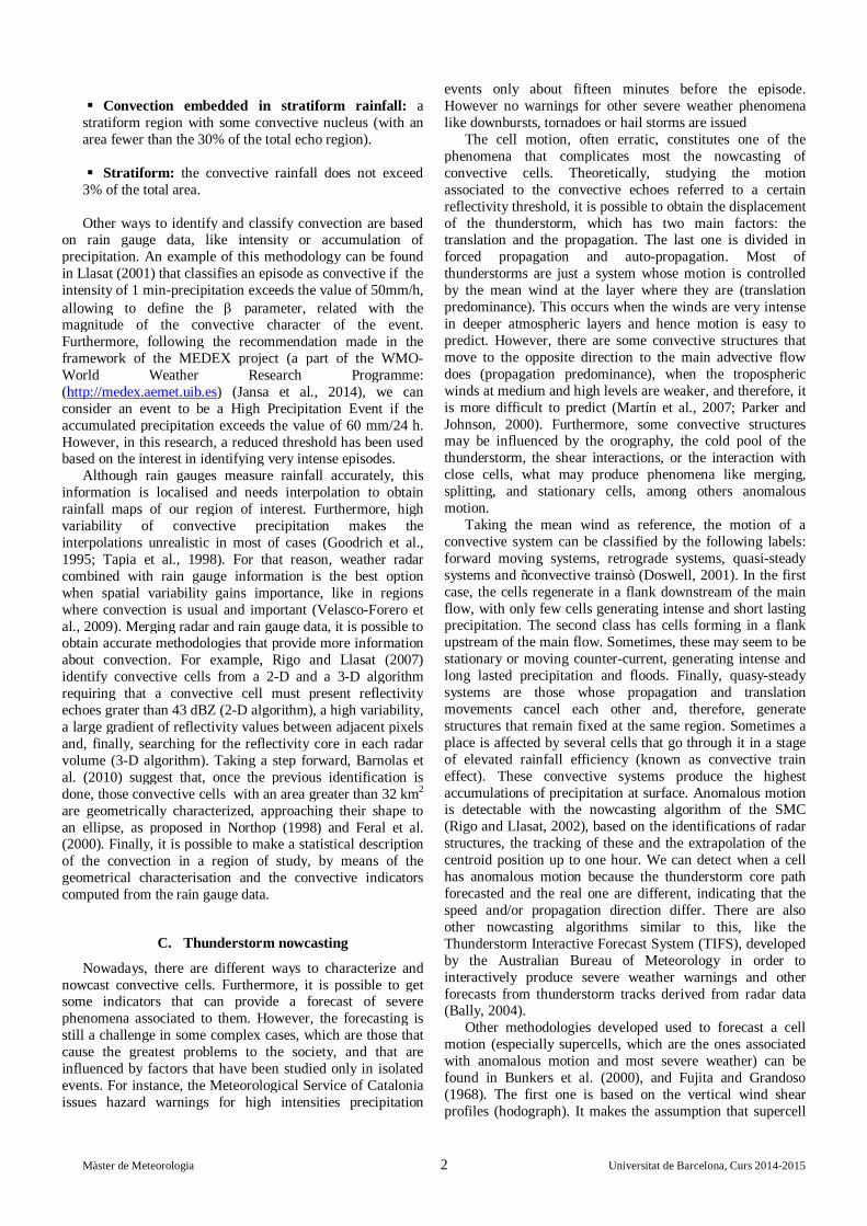
One of the most important radar products are the CAPPI levels (Constant Altitude Plan Position Indicator). These are horizontal cuts of interpolated data at a fixed altitude, obtained from a set of PPI (Plan Position Indicator), that refer to reflectivity data at a constant elevation angle. The product used in this work is a composite of 10 (from 1 to 10 km) short-range CAPPI (150 km) generated combining the volumes obtained from each radar with a spatial resolution of 2x2 km² and a temporal resolution of six minutes (Rigo et al., 2008). Fig. (2) shows the situation and the coverage of the XRAD network in short volumetric product and long range scans. The latter is a single PPI scan at 0.6º elevation and reaching 250 km range that is used.
Figure 2: Radar coverage of the SMC network, showing long and short range coverage.
The daily rainfall chart resulting from a compound
product of radar and rain gauge data have also been used as additional data source in the present study. This product is computed every day by means of the algorithms developed
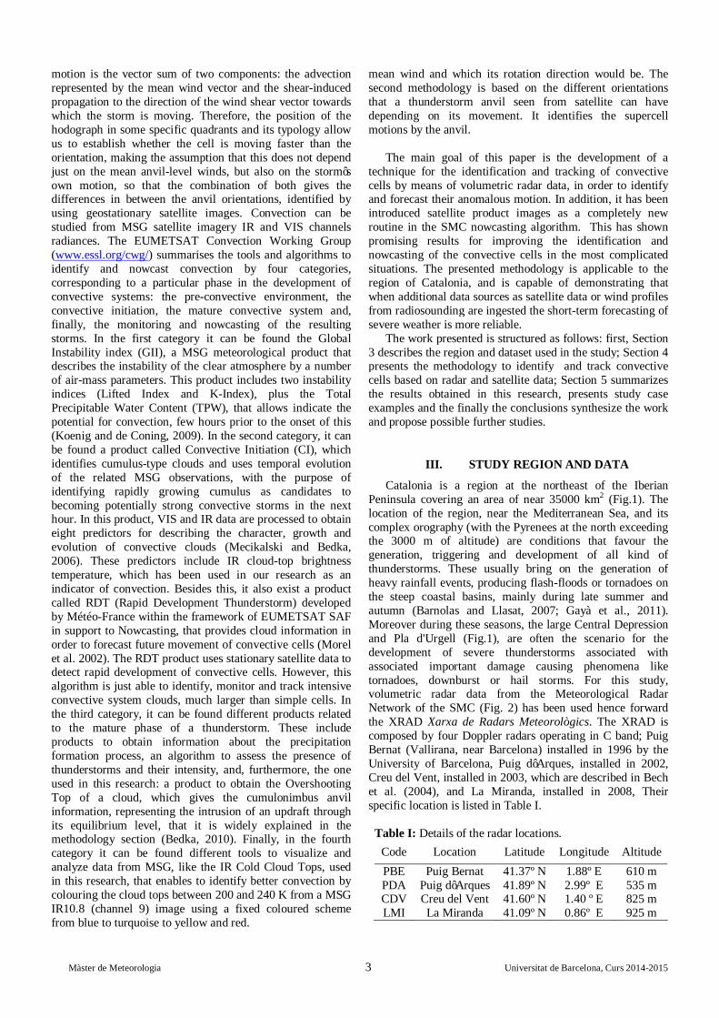
by the SMC, using the XRAD and XEMA (Xarxa d’Estacions Meteorològiques Automàtiques) data. The rain gauge network of the SMC is integrated into the 180 automatic meteorological stations, distributed by the entire region, how it is shown in Fig. (3). The rain gauges have a minimum threshold of detection of 0.1 mm. Data collected is recorded each 30 minutes and send to the SMC every half an hour by using GPRS (General Packet Radio Service) communications.
Figure 3: Automatic Meteorological Stations Network, XEMA (Xarxa d’Estacions Meteorològiques Automàtiques) of the SMC.
MSG (Meteosat Second Generation) satellite data has
also been processed for this research. This data is stored at the SMC since 2005, and has been used to test the proposed methodology. The MSG-10 is the main mission of the Meteosat Second Generation satellites and comprises High
Màster de Meteorologia 5 Universitat de Barcelona, Curs 2014-2015
Rate SEVIRI image data of the satellite’s field of view in 12 spectral bands. These image data sets consist of geographical arrays of image pixels of various sizes. Each pixel contains 10 data bits, representing the received radiation from the Earth and its atmosphere in the 12 spectral channels; 11 of these provide measurements with a resolution of 3 km at the sub-satellite point and an extra one, the High Resolution Visible (HRV) channel, which provides measurements with a resolution of 1 km. Table II lists the 12 spectral channels of the MSG-10 satellite and the main observational application of each channel (Schmetz et al., 2002).
Table II: List of the spectral channels of the MSG-10.
Channel number
Spectral Band (μm)
Main observational application
1 VIS 0.6 Surface, clouds, wind fields
2 VIS 0.8 Surface, clouds, wind fields
3 NIR 1.6 Surface, cloud phase
4 IR 3.9 Surface, clouds, wind fields
5 WV 6.2 Water vapour, high
level clouds, atmospheric instability
6 WV 7.3 Water vapour, atmospheric instability
7 IR 8.7 Surface, clouds, atmospheric instability
8 IR 9.7 Ozone
9 IR 10.8 Surface, clouds, wind
fields, atmospheric instability
10 IR 12.0 Surface, clouds, atmospheric instability
11 IR 13.4 Cirrus cloud height, atmospheric instability
12 HRV broadband ( 0.4 -1.1 ) Surface, clouds
Currently the SMC receives MSG-10 (nominal satellite)
encrypted images every 15 minutes and MSG-9 (rapid scan satellite) every 5 minutes. The MSG-10 and MSG-9 satellites are geostationary orbiting at 36000 km height above the equator and placed 0º and 9.5 º East respectively from the Greenwich meridian. Both satellites scan Europe, Africa and adjacent seas. RSS scans a third part of the Earth disc and therefore the scan repetition time is a third of that of the MSG-10 satellite providing images with more frequency (every 5 minutes). At the SMC only channels 5 and 9 from RSS service are recorded and together with the 0º MSG-10 images go through a calibration process. This process converts counts (binary pixel values) into radiances, radiances into brightness temperature, and finally projects the image to a georeference system of coordinates. This process will be widely explained in the next section. In this study satellite images of channels there 9 (IR) and 5 (WV) have been processed in order to extract images of the
overshooting tops of the clouds, their brightness temperature and their height.
Finally to calculate the cloud height from satellite images the Barcelona atmospheric sounding from the SMC has been used. The atmospheric sounding is automatically launched every day at 00 and 12 UTC from the Physics Faculty building roof of the University of Barcelona and is integrated into the WMO atmospheric sounding network (08190). In particular case that will be described in the results section a virtual atmospheric sounding based on an ICAO Standard Atmosphere has also been used (Cavcar, 2000).
This study is focused on the years 2013 and 2014. In this period an average of about 40 thunderstorms days per year have been recorded in Catalonia (Pineda et al., 2011).
IV. METHODOLOGY
All the algorithms developed in the present study have been developed using the programming environment R-Cran (R-Cran Team, 2013), for data and image processing. R is a free software environment for statistical computing and graphics that compiles and runs on a wide variety of platforms. It is an official part of the Free Software Foundation’ GNU.
The steps followed to analyse and identify the anomalous motion of storms have been classified by according to the type of data analyzed (rain gauge, radar and satellite), and, also, by the processes used in any case.
A. Previous classification from accumulated precipitation data
In order to obtain a fast classification of the 24 hours accumulated precipitation data base of 2013 and 2014, a series of filters have been applied to classify daily rainfall charts in days with no rain, with non-convective rain and with convective rain. This has been a very quick way to identify possible cases of convection, taking into account that there is a lot of imagery to analyze, and the procedures of identification of convection require some time. It has been a good way to exclude days without precipitation or with little precipitation, even more, to identify cases of convection, unless, in this study, it has been done a more exhaustive identification for convection. Those days with both kinds of precipitation have been classified as “potentially convective” because it is the one with the highest intensity. All the techniques used in this paper has been applied only in those cases catalogued as “potentially convective”.
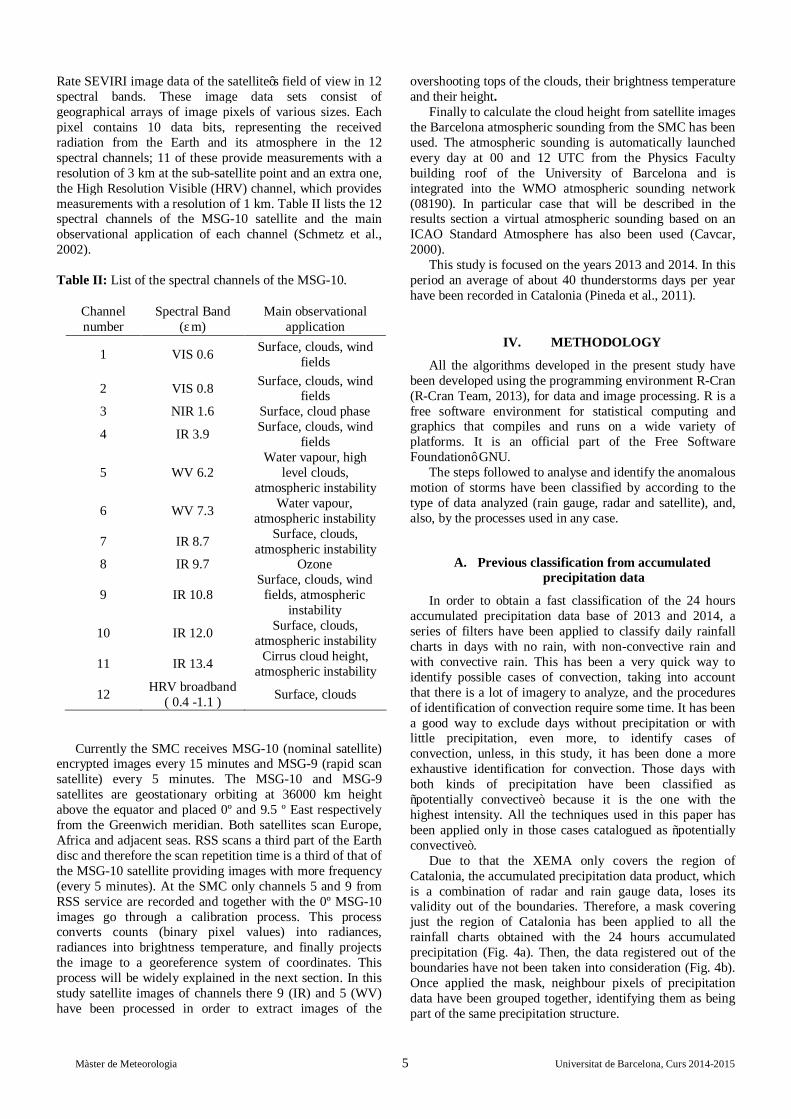
Due to that the XEMA only covers the region of Catalonia, the accumulated precipitation data product, which is a combination of radar and rain gauge data, loses its validity out of the boundaries. Therefore, a mask covering just the region of Catalonia has been applied to all the rainfall charts obtained with the 24 hours accumulated precipitation (Fig. 4a). Then, the data registered out of the boundaries have not been taken into consideration (Fig. 4b). Once applied the mask, neighbour pixels of precipitation data have been grouped together, identifying them as being part of the same precipitation structure.
Màster de Meteorologia 6 Universitat de Barcelona, Curs 2014-2015
Figure 4: 24 hours accumulated rainfall chart for the 17th August 2013: (a) area covered by the XRAD; (b) rainfall chart only for the region of Catalonia.
A preliminary classification has been applied to each daily precipitation chart following the criteria showed in Table III.
Table III: Precipitation and extension thresholds imposed to the daily rainfall charts.
p = 0 (mm)
0 ≤ p <1 (mm)
1≤ p <15 (mm)
p ≥ 15 (mm)
A<20 km2 No rain No rain Non-conv. Conv.
A≥20 km2 No rain Non-conv. Non-conv. Conv.
First, those days that have not presented any structure in
24 hours, have been catalogued as “no rain” days. Secondly, those days that have presented some kind of precipitation structure but with accumulated precipitation smaller or equal than 1 mm and a continuous extension of 20 pixels (20 km2) or less, have been also catalogued as “no rain”. This extension restriction has been done in order to distinguish those days that have presented some kind of precipitation due to fog or dew, but that can’t be considered precipitation from clouds. Thirdly, those days that have presented structures with 24 hours accumulated precipitation greater than 1 mm and less or equal than 15 mm, with an extension greater than 20 km 2 have been catalogued as “non-convective”. Finally, those days that have presented a maximum of accumulated precipitation greater than 15 mm, have been catalogued as “potentially convective”.
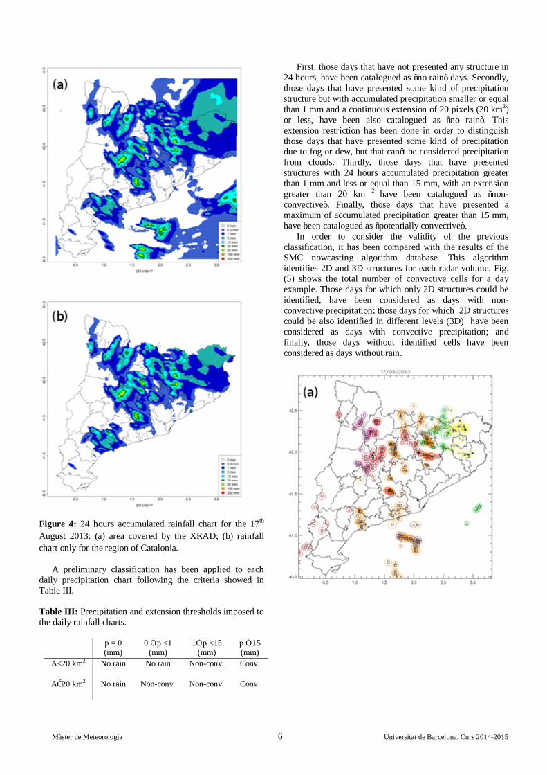
In order to consider the validity of the previous classification, it has been compared with the results of the SMC nowcasting algorithm database. This algorithm identifies 2D and 3D structures for each radar volume. Fig. (5) shows the total number of convective cells for a day example. Those days for which only 2D structures could be identified, have been considered as days with non-convective precipitation; those days for which 2D structures could be also identified in different levels (3D) have been considered as days with convective precipitation; and finally, those days without identified cells have been considered as days without rain.
Màster de Meteorologia 7 Universitat de Barcelona, Curs 2014-2015
Figure 5: Convective cells identified by the nowcasting algorithm of the SMC for the 17th August 2013: (a) area covered by the XRAD; (b) convective cells only for the region of Catalonia.
Once it has been made the previous classification of all
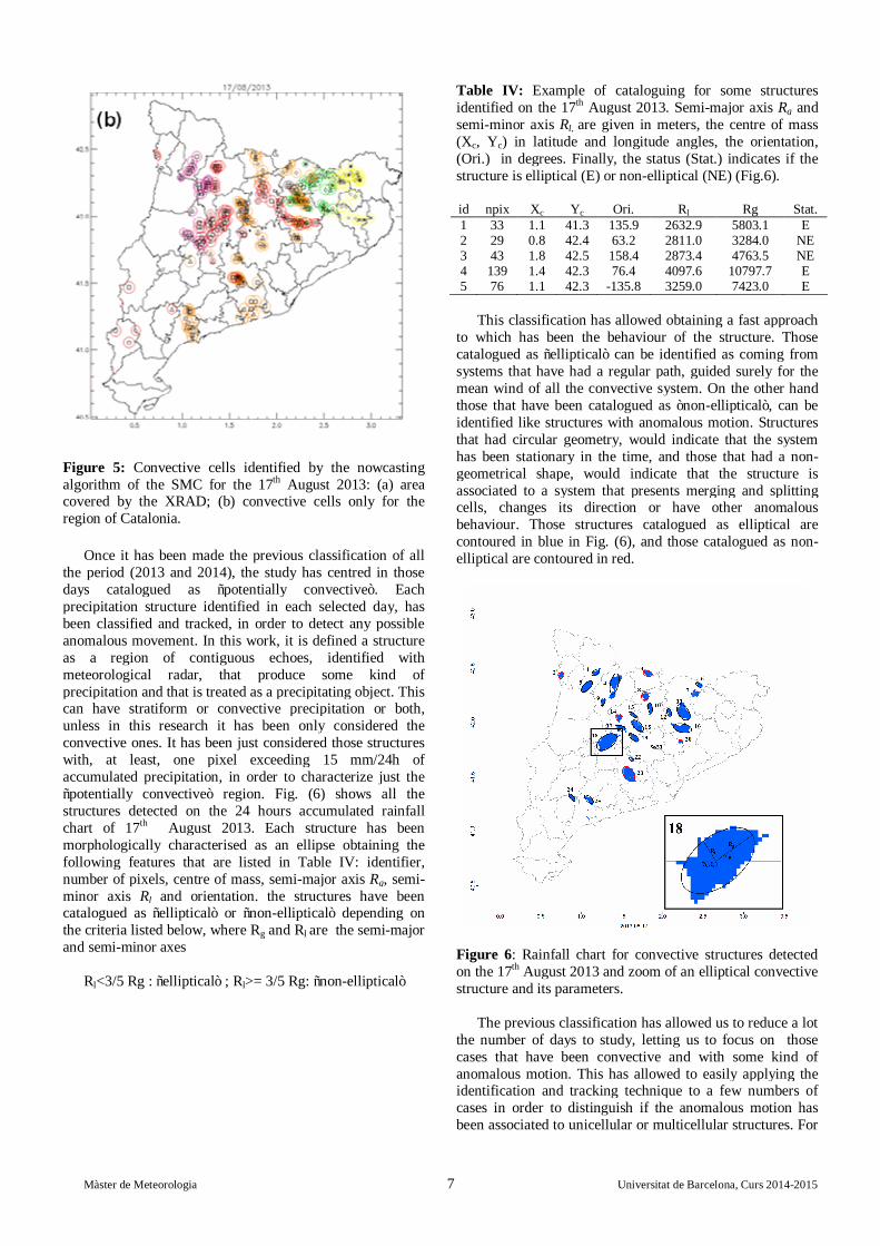
the period (2013 and 2014), the study has centred in those days catalogued as “potentially convective”. Each precipitation structure identified in each selected day, has been classified and tracked, in order to detect any possible anomalous movement. In this work, it is defined a structure as a region of contiguous echoes, identified with meteorological radar, that produce some kind of precipitation and that is treated as a precipitating object. This can have stratiform or convective precipitation or both, unless in this research it has been only considered the convective ones. It has been just considered those structures with, at least, one pixel exceeding 15 mm/24h of accumulated precipitation, in order to characterize just the “potentially convective” region. Fig. (6) shows all the structures detected on the 24 hours accumulated rainfall chart of 17th August 2013. Each structure has been morphologically characterised as an ellipse obtaining the following features that are listed in Table IV: identifier, number of pixels, centre of mass, semi-major axis Rg, semi-minor axis Rl and orientation. the structures have been catalogued as “elliptical” or “non-elliptical” depending on the criteria listed below, where Rg and Rl are the semi-major and semi-minor axes
Rl<3/5 Rg : “elliptical” ; Rl>= 3/5 Rg: “non-elliptical”
Table IV: Example of cataloguing for some structures identified on the 17th August 2013. Semi-major axis Rg and semi-minor axis Rl, are given in meters, the centre of mass (Xc, Yc) in latitude and longitude angles, the orientation, (Ori.) in degrees. Finally, the status (Stat.) indicates if the structure is elliptical (E) or non-elliptical (NE) (Fig.6). id npix Xc Yc Ori. Rl Rg Stat. 1 33 1.1 41.3 135.9 2632.9 5803.1 E 2 29 0.8 42.4 63.2 2811.0 3284.0 NE 3 43 1.8 42.5 158.4 2873.4 4763.5 NE 4 139 1.4 42.3 76.4 4097.6 10797.7 E 5 76 1.1 42.3 -135.8 3259.0 7423.0 E
This classification has allowed obtaining a fast approach
to which has been the behaviour of the structure. Those catalogued as “elliptical” can be identified as coming from systems that have had a regular path, guided surely for the mean wind of all the convective system. On the other hand those that have been catalogued as ”non-elliptical”, can be identified like structures with anomalous motion. Structures that had circular geometry, would indicate that the system has been stationary in the time, and those that had a non- geometrical shape, would indicate that the structure is associated to a system that presents merging and splitting cells, changes its direction or have other anomalous behaviour. Those structures catalogued as elliptical are contoured in blue in Fig. (6), and those catalogued as non-elliptical are contoured in red.
Figure 6: Rainfall chart for convective structures detected on the 17th August 2013 and zoom of an elliptical convective structure and its parameters.
The previous classification has allowed us to reduce a lot the number of days to study, letting us to focus on those cases that have been convective and with some kind of anomalous motion. This has allowed to easily applying the identification and tracking technique to a few numbers of cases in order to distinguish if the anomalous motion has been associated to unicellular or multicellular structures. For
Màster de Meteorologia 8 Universitat de Barcelona, Curs 2014-2015
those paths that have been considered as normal, it has been tried to consider if they are really described by one single cell or are different cells that have appeared separately in time.
Once this methodology has been applied to the whole database, a 3-D identification of radar structures has been applied to the selected sample.
B. 3-D identification of radar structures and tracking
In order to identify convective structures and track its path, it has been used an algorithm developed by Johnson et al. (1998) to detect 3-D radar structures, known as SCIT (Storm Cell Identification and Tracking). This algorithm was adapted to the Spanish area by Carretero et al. (2001), and also to the Catalan region by Rigo and Llasat (2002). In this paper, the algorithm has been slightly modified, in order to make some improvements.
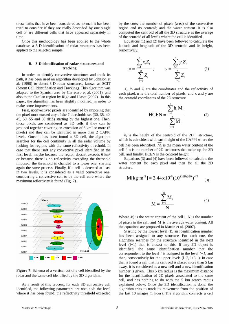
First, “convective” pixels are identified by imposing that the pixel must exceed any of the 7 thresholds set (30, 35, 40, 45, 50, 55 and 60 dBZ) starting by the highest one. Then, those pixels are considered as 3D cells if they can be grouped together covering an extension of 6 km² or more (6 pixels) and they can be identified in more than 2 CAPPI levels. Once it has been found a 3D cell, the algorithm searches for the cell continuity in all the radar volume by looking for regions with the same reflectivity threshold. In case that there isn’t any convective pixel identified in the first level, maybe because the region doesn't exceeds 6 km² or because there is no reflectivity exceeding the threshold imposed, the threshold is changed to a lower one, starting again the same process. Finally, if a cell is detected at least in two levels, it is considered as a valid convective one, considering a convective cell to be the cell core where the maximum reflectivity is found (Fig. 7).
Figure 7: Schema of a vertical cut of a cell identified by the radar and the same cell identified by the 3D algorithm.
As a result of this process, for each 3D convective cell identified, the following parameters are obtained: the level where it has been found; the reflectivity threshold exceeded
by the core; the number of pixels (area) of the convective region and its centroid; and the water content. It is also computed the centroid of all the 3D structure as the average of the centroid of all levels where the cell is identified.
Equations (1) and (2) have been followed to calculate the latitude and longitude of the 3D centroid and its height, respectively.
Xi, Yi and Zi are the coordinates and the reflectivity of
each pixel, n is the total number of pixels, and x and y are the centroid coordinates of the 2D structure.
hi is the height of the centroid of the 2D i structure,
which is coincident with each height of the CAPPI where the cell has been identified. iM is the mean water content of the cell i, n is the number of 2D structures that make up the 3D cell, and finally, HCEN is the centroid height.
Equations (3) and (4) have been followed to calculate the water content for each pixel and then for all the 2D structure:
-3 -6 Z[dBz]/10 4/7M[kg·m ] = 3.44x10 (10 ) (3)
N
ii 1
MM
N==∑ (4)
Where Mi is the water content of the cell i, N is the number of pixels in the cell, and M is the average water content. All the equations are proposed in Martin et al. (2007).
Starting by the lowest level (l), an identification number has been assigned to any structure. For each one, the algorithm searches for the structure identified in the next level (l+1) that is closest to this. If any 2D object is identified, the same identification number that the correspondent to the level l is assigned to the level l+1, and then, consecutively for the upper levels (l+2, l+3,..). In case that is found a cell that its centroid is placed more than 5 km away, it is considered as a new cell and a new identification number is given. This 5 km radius is the maximum distance for the identification of 2D pixels associated to the same cell, and has nothing to do with the 5 km search radius explained below. Once the 3D identification is done, the algorithm tries to track its movement from the position of the last 10 images (1 hour). The algorithm connects a cell
1
1
=
=
=∑
∑
n
i ii
n
ii
x Zx
Z ; 1
1
=
=
=∑
∑
n
i ii
n
ii
y Zy
Z (1)
n
iii 1
n
ii 1
h MHCEN
M
=
=
=∑
∑ (2)
Màster de Meteorologia 9 Universitat de Barcelona, Curs 2014-2015
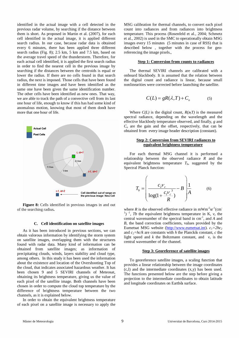
identified in the actual image with a cell detected in the previous radar volume, by searching if the distance between them is short. As proposed in Martin et al. (2007), for each cell identified in the actual image, it is applied different search radius. In our case, because radar data is obtained every 6 minutes, there has been applied three different search radius (Fig. 8); 2.5 km, 5 km and 7.5 km, based on the average travel speed of the thunderstorm. Therefore, for each actual cell identified, it is applied the first search radius in order to find the nearest cell in the previous image by searching if the distances between the centroids is equal or lower the radius. If there are no cells found in that search radius, the next is imposed. Those cells that have been found in different time images and have been identified as the same one have been given the same identification number. The other cells have been identified as new ones. That way, we are able to track the path of a convective cell from its last one hour of life, enough to know if this has had some kind of anomalous motion, knowing that most of them don’t have more that one hour of life.
Figure 8: Cells identified in previous images in and out
of the searching radius.
C. Cell identification on satellite images
As it has been introduced in previous sections, we can obtain valorous information by identifying the storm system on satellite images, overlapping them with the structures found with radar data. Many kind of information can be obtained from satellite images; as information of precipitating clouds, winds, layers stability and cloud type, among others. In this study it has been used the information about the existence and location of the Overshooting Top of the cloud, that indicates associated hazardous weather. It has been chosen 9 and 5 SEVIRI channels of Meteosat, obtaining its brightness temperature, giving us the value of each pixel of the satellite image. Both channels have been chosen in order to compute the cloud top temperature by the difference of brightness temperature between the two channels, as it is explained below.
In order to obtain the equivalent brightness temperature of each pixel on a satellite image is necessary to apply the
MSG calibration for thermal channels, to convert each pixel count into radiances and from radiances into brightness temperature. This process (Rosenfeld et al., 2004; Schmetz et al., 2002) is used in the SMC to operationally obtain MSG images every 15 minutes (5 minutes in case of RSS) that is described below , together with the process for geo-referencing the image pixels.,
Step 1: Conversion from counts to radiances
The thermal SEVIRI channels are calibrated with a
onboard blackbody. It is assumed that the relation between the digital count and radiance is linear, because small nonlinearities were corrected before launching the satellite.
( ) ( , ) oC L gR T Cλ= + (5)
Where C(L) is the digital count, R(λ,T) is the measured
spectral radiance, depending on the wavelength and the effective blackbody temperature observed, and finally, g and Co are the gain and the offset, respectively, that can be obtained from every image header description (constant).
Step 2: Conversion from SEVIRI radiances to
equivalent brightness temperature For each thermal MSG channel it is performed a
relationship between the observed radiance R and the equivalent brightness temperature Tb, suggested by the Spectral Planck function:
23
1
1
log(1 )
cb
c
cT Bc A
R
νν
= − +
(6)
where R is the observed effective radiance in mWm-2sr-1(cm-
1) -1, Tb the equivalent brightness temperature in K, vc the central wavenumber of the spectral band in cm-1, and A and B, the band correction coefficients, values provided by the Eumetsat MSG website (http://www.eumetsat.int). c1=2hc2 and c2=hc/k are constants with h the Planck’s constant, c the light speed and k the Boltzmann constant, and vc is the central wavenumber of the channel.
Step 3: Georeference of satellite images
To georeference satellite images, a scaling function that
provides a linear relationship between the image coordinates (c,l) and the intermediate coordinates (x,y) has been used. The functions presented below are the step before giving a projection to the intermediate coordinates to obtain latitude and longitude coordinates on Earth’s surface.
Màster de Meteorologia 10 Universitat de Barcelona, Curs 2014-2015
16
16
nint( 2 )nint( 2 )
c COFF x CFACl LOFF y LFAC
−
−
= +
= + (7)
Here, COFF, CFAC, LFAC and LOFF are scaling
coefficients provided by the image navigation record, and “nint” denotes “the nearest integer”. Once obtained the intermediate coordinates it is possible to obtain the longitude and latitude coordinates by applying some projection functions detailed in the LRIT/HRIT Global Specifications document of the Coordination Group for Meteorological Satellites (Wolf and Just, 1999). These functions depend on the projection desired, in our case, the Normalized Geostationary Projection.
a. Overshooting The Overshooting Top of a cloud is the appearance of
the existence of deep convective updraft cores that are able to rise above the storms' equilibrium level in the tropopause and penetrate into the stratosphere (Bedka, 2010). If a thunderstorm has an Overshooting Top, it is an indication of associated severe weather at the Earth's surface (Bedka, 2010; Brunner et al., 2007; Reynols, 1980), turbulence and Cloud to Ground lightning in the thunderstorm (Machado et al., 2009).
In this study the methodology of the SMC for computing the Overshooting Tops combining the infrared channel 9 (IR: 10.5 μm) and the water vapour absorption channel 5 (WV: 5.7 μm) brightness temperature has been applied. It is based on this one proposed by Schmetz et al. (1997), computing the cloud top temperature by the difference of brightness temperature between the two channels. Simultaneous observations of cloudy pixels in both channels of Meteosat shows that the equivalent brightness temperature in WV channel can be, as much as 6-8 K larger than IR channel due to the stratospheric water vapour absorbing radiation from the cold cloud top, emitting at higher stratospheric temperatures. This brightness temperature difference depends on the amount of water vapour, the temperature lapse rate in the stratosphere, and it is bigger when the cloud top is in the region of temperature inversion in the troposphere (Schmetz et al., 1997). The temperature of the Overshooting Top of the cloud, Tb, is then computed as the difference between the WV channel 5 and the IR channel 9 equivalent brightness temperatures as shown below:
WV IRb b bT T T= − (8)
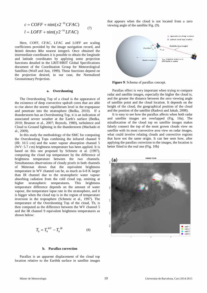
b. Parallax correction Parallax is an apparent displacement of the cloud top
location relative to the Earth’s surface in satellite images
that appears when the cloud is not located from a zero viewing angle of the satellite Fig. (9).
Figure 9: Schema of parallax concept. Parallax effect is very important when trying to compare
radar and satellite images, especially the higher the cloud is, and the greater the distance between the zero viewing angle of satellite point and the cloud location. It depends on the height of the cloud, the geographical position of the cloud and the position of the satellite (Radová and Jakub, 2008).
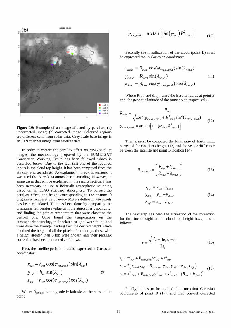
It is easy to see how the parallax affects when both radar and satellite images are overlapped (Fig. 10a). The misallocation of the cloud top on satellite images makes falsely connect the top of the most grown clouds view on satellite with its most convective area view on radar images, what could involve relating clouds and convective regions that have not the same origin. It can bee seen how, after applying the parallax correction to the images, the location is better fitted to the real one (Fig. 10b)
Màster de Meteorologia 11 Universitat de Barcelona, Curs 2014-2015
Figure 10: Example of an image affected by parallax; (a) uncorrected image; (b) corrected image. Coloured regions are different cells from radar data. Grey scale base image is an IR 9 channel image from satellite data.
In order to correct the parallax effect on MSG satellite
images, the methodology proposed by the EUMETSAT Convection Working Group has been followed which is described below. Due to the fact that one of the required inputs is the cloud top height, it has been computed from the atmospheric soundings. As explained in previous sections, it was used the Barcelona atmospheric sounding. However, in some cases that will be explained in the results section, it has been necessary to use a “virtual” atmospheric sounding based on an ICAO standard atmosphere. To correct the parallax effect, the height corresponding to the channel 9 brightness temperature of every MSG satellite image pixels has been calculated. This has been done by comparing the brightness temperature value with the atmospheric sounding, and finding the pair of temperature that were closer to the desired one. Once found the temperatures on the atmospheric sounding, their related heights were found and were done the average, finding then the desired height. Once obtained the height of all the pixels of the image, those with a height greater than 5 km were chosen and their parallax correction has been computed as follows.
First, the satellite position must be expressed in Cartesian
coordinates:
,
,
cos( )sin( )
sin( )cos( )cos( )
sat sat sat geod sat
sat sat sat
sat sat sat geod sat
x h
y hz h
ϕ λ
λϕ λ
=
=
=
(9)
Where φsat,geod is the geodetic latitude of the subsatellite
point:
( ) 2, arctan tansat geod sat ratioRϕ ϕ =
(10)
Secondly the misallocation of the cloud (point B) must
be expressed too in Cartesian coordinates:
,
,
cos( )sin( )sin( )cos( )cos( )
cloud local cloud geod cloud
cloud local cloud
cloud local cloud geod cloud
x Ry Rz R
ϕ λ
λϕ λ
=
=
=
(11)
Where Rlocal and φsat,cloud are the Earth’s radius at point B
and the geodetic latitude of the same point, respectively :
2 2 2, ,
2,
cos ( ) sin ( )
arctan tan( )
eqlocal
cloud geod ratio cloud geod
cloud geod cloud ratio
RR
R
R
ϕ ϕ
ϕ ϕ
=+
=
(12)
Then it must be computed the local ratio of Earth radii,
corrected for cloud top height (13) and the vector difference between the satellite and point B location (14).
2
,equ cloud
ratio localpole cloud
R hR
R h +
= + (13)
diff sat cloud
diff sat cloud
diff sat cloud
x x x
y y y
z z z
= −
= −
= −
(14)
The next step has been the estimation of the correction
for the line of sight at the cloud top height hcloud, as it follows:
22 1 3 2
1
42
e e e ec
e− −
= (15)
( )2 2 2
1 ,
2 ,
2 2 2 23 ,
2
( )
diff ratio local diff diff
cloud diff ratio local cloud diff cloud diff
cloud ratio local cloud cloud equ cloud
e x R y z
e x x R y y z z
e x R y z R h
= + +
= + +
= + + − +(16)
Finally, it has to be applied the correction Cartesian
coordinates of point B (17), and then convert corrected

Màster de Meteorologia 12 Universitat de Barcelona, Curs 2014-2015
Cartesian coordinates back to latitude and longitude to find the corrected cloud sight (point A) (18, 19 and 20).
corr cloud diff
corr cloud diff
corr cloud diff
x x cx
y y cy
z z cz
= −
= −
= −
(17)
2 2
, 2
,
tan arctan
arctan
tan( )
corr
corr corrcloud corr
ratio
corrcloud corr
corr
yx z
R
xz
ϕ
λ
+ =
=
(18) (19)
, 2( )cloud corr corr corrATAN x yλ = (20)
ATAN2 is the arctangent function with two arguments, gathering information on the signs of the inputs to return the appropriate quadrant of the computed angle.
V. RESULTS
The following section has been structured in two main
parts. The first one shows climatology of the daily accumulated precipitation fields of 2013 and 2014, in which a total of 730 daily accumulated rainfall data has been analysed. The second one analyses the anomalous movement from the volumetric radar data and MSG imagery, with images every 6 minutes of the study cases.
A. Precipitation patterns
As it has been explained in the previous section, the classification has been done with the goal of better selecting the convective days to study, and getting a fast idea of the typology of the precipitation chart and the morphology of the structures found. The classification, developed in the present work and explained in the Methodology, has been compared with the SMC convective cell data base identified with the nowcasting algorithm. Table IV shows the verification scores, where it has been considered that the observed events are the results obtained with the SMC nowcasting algorithm and the forecasted events are the results obtained with our classification nowcasting algorithm and the forecasted events are the results obtained with our classification.
Table IV: Verification scores for the classification proposed here method.
Accuracy POD FAR 0.71 0.83 0.33
As it can be seen, the accuracy and the POD (Probablity
Of Detection) scores are close to 1 (perfect), which means that most of the observed “convective rain days”, “not convective rain days” and “no rain days” with the SMC nowcasting algorithm, where correctly forecasted by our methodology, based on accumulated precipitation data. One of the facts which caused not having a perfect forecasting is that the SMC nowcasting algorithm considers all the radar coverage while in our methodology it is just considered the region of Catalonia. Then some of the days that we have been considered as “no rain days” or “not convective rain days”, could be considered as convective ones by the SMC algorithm due to the presence of a convective core at the sea or out of the Catalonia boundaries. On the other hand we are not strictly comparing with “observed” data, but with the results from another algorithm that uses other inputs.
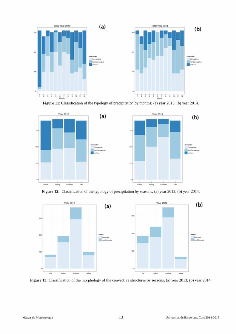
Once accepted the methodology to classify daily rainfall patterns, the main features of the precipitation structures has been analysed at monthly and seasonal scale. Fig. (11a) and Fig. (11b) show the typology of the precipitation by months for the year 2013 and 2014. Fig. (12a) and Fig. (12b) show the typology of the precipitation by seasons for the same years studied. Fig. (13a) and Fig. (13b) show a classification of the morphology of the convective structures by seasons, to identify which pattern is the most common followed by thunderstorms in the region of Catalonia, and finally, Fig.(14a) and Fig.(14b) show the convective rainfall distribution for the Catalonia region, in order to identify which areas are more affected by convective rain. All figures are discussed below.
Màster de Meteorologia 13 Universitat de Barcelona, Curs 2014-2015
Figure 11: Classification of the typology of precipitation by months; (a) year 2013; (b) year 2014.
Figure 12: Classification of the typology of precipitation by seasons; (a) year 2013; (b) year 2014.
Figure 13: Classification of the morphology of the convective structures by seasons; (a) year 2013; (b) year 2014.
Màster de Meteorologia 14 Universitat de Barcelona, Curs 2014-2015
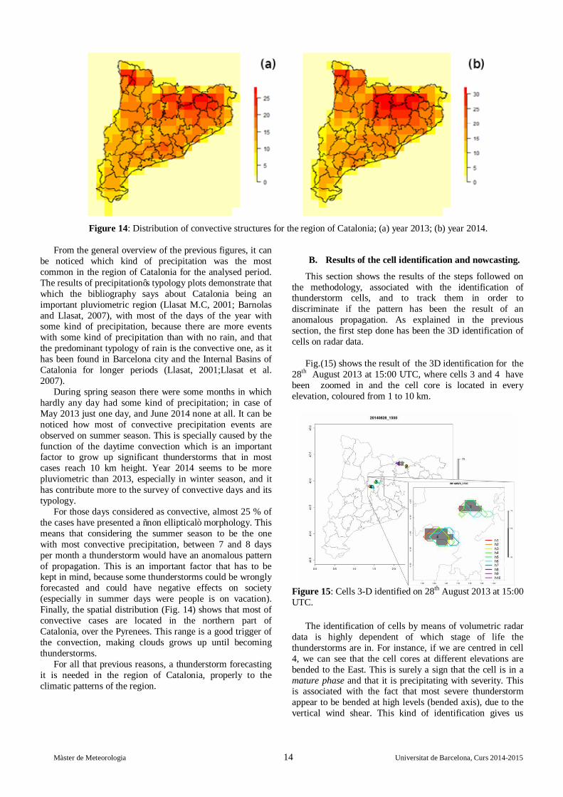
Figure 14: Distribution of convective structures for the region of Catalonia; (a) year 2013; (b) year 2014.
From the general overview of the previous figures, it can
be noticed which kind of precipitation was the most common in the region of Catalonia for the analysed period. The results of precipitation’s typology plots demonstrate that which the bibliography says about Catalonia being an important pluviometric region (Llasat M.C, 2001; Barnolas and Llasat, 2007), with most of the days of the year with some kind of precipitation, because there are more events with some kind of precipitation than with no rain, and that the predominant typology of rain is the convective one, as it has been found in Barcelona city and the Internal Basins of Catalonia for longer periods (Llasat, 2001;Llasat et al. 2007).
During spring season there were some months in which hardly any day had some kind of precipitation; in case of May 2013 just one day, and June 2014 none at all. It can be noticed how most of convective precipitation events are observed on summer season. This is specially caused by the function of the daytime convection which is an important factor to grow up significant thunderstorms that in most cases reach 10 km height. Year 2014 seems to be more pluviometric than 2013, especially in winter season, and it has contribute more to the survey of convective days and its typology.
For those days considered as convective, almost 25 % of the cases have presented a “non elliptical” morphology. This means that considering the summer season to be the one with most convective precipitation, between 7 and 8 days per month a thunderstorm would have an anomalous pattern of propagation. This is an important factor that has to be kept in mind, because some thunderstorms could be wrongly forecasted and could have negative effects on society (especially in summer days were people is on vacation). Finally, the spatial distribution (Fig. 14) shows that most of convective cases are located in the northern part of Catalonia, over the Pyrenees. This range is a good trigger of the convection, making clouds grows up until becoming thunderstorms.
For all that previous reasons, a thunderstorm forecasting it is needed in the region of Catalonia, properly to the climatic patterns of the region.
B. Results of the cell identification and nowcasting.
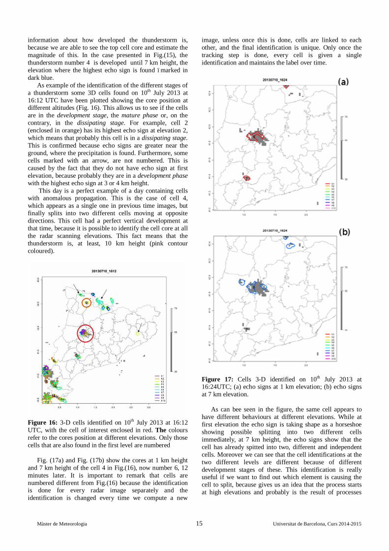
This section shows the results of the steps followed on the methodology, associated with the identification of thunderstorm cells, and to track them in order to discriminate if the pattern has been the result of an anomalous propagation. As explained in the previous section, the first step done has been the 3D identification of cells on radar data.
Fig.(15) shows the result of the 3D identification for the
28th August 2013 at 15:00 UTC, where cells 3 and 4 have been zoomed in and the cell core is located in every elevation, coloured from 1 to 10 km.
Figure 15: Cells 3-D identified on 28th August 2013 at 15:00 UTC.
The identification of cells by means of volumetric radar
data is highly dependent of which stage of life the thunderstorms are in. For instance, if we are centred in cell 4, we can see that the cell cores at different elevations are bended to the East. This is surely a sign that the cell is in a mature phase and that it is precipitating with severity. This is associated with the fact that most severe thunderstorm appear to be bended at high levels (bended axis), due to the vertical wind shear. This kind of identification gives us
Màster de Meteorologia 15 Universitat de Barcelona, Curs 2014-2015
information about how developed the thunderstorm is, because we are able to see the top cell core and estimate the magnitude of this. In the case presented in Fig.(15), the thunderstorm number 4 is developed until 7 km height, the elevation where the highest echo sign is found –marked in dark blue.
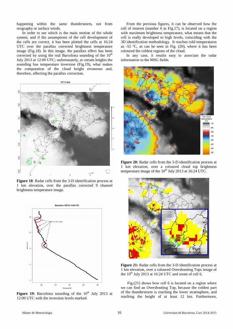
As example of the identification of the different stages of a thunderstorm some 3D cells found on 10th July 2013 at 16:12 UTC have been plotted showing the core position at different altitudes (Fig. 16). This allows us to see if the cells are in the development stage, the mature phase or, on the contrary, in the dissipating stage. For example, cell 2 (enclosed in orange) has its highest echo sign at elevation 2, which means that probably this cell is in a dissipating stage. This is confirmed because echo signs are greater near the ground, where the precipitation is found. Furthermore, some cells marked with an arrow, are not numbered. This is caused by the fact that they do not have echo sign at first elevation, because probably they are in a development phase with the highest echo sign at 3 or 4 km height.
This day is a perfect example of a day containing cells with anomalous propagation. This is the case of cell 4, which appears as a single one in previous time images, but finally splits into two different cells moving at opposite directions. This cell had a perfect vertical development at that time, because it is possible to identify the cell core at all the radar scanning elevations. This fact means that the thunderstorm is, at least, 10 km height (pink contour coloured).
Figure 16: 3-D cells identified on 10th July 2013 at 16:12 UTC, with the cell of interest enclosed in red. The colours refer to the cores position at different elevations. Only those cells that are also found in the first level are numbered
Fig. (17a) and Fig. (17b) show the cores at 1 km height
and 7 km height of the cell 4 in Fig.(16), now number 6, 12 minutes later. It is important to remark that cells are numbered different from Fig.(16) because the identification is done for every radar image separately and the identification is changed every time we compute a new
image, unless once this is done, cells are linked to each other, and the final identification is unique. Only once the tracking step is done, every cell is given a single identification and maintains the label over time.
Figure 17: Cells 3-D identified on 10th July 2013 at 16:24UTC; (a) echo signs at 1 km elevation; (b) echo signs at 7 km elevation.
As can bee seen in the figure, the same cell appears to
have different behaviours at different elevations. While at first elevation the echo sign is taking shape as a horseshoe showing possible splitting into two different cells immediately, at 7 km height, the echo signs show that the cell has already spitted into two, different and independent cells. Moreover we can see that the cell identifications at the two different levels are different because of different development stages of these. This identification is really useful if we want to find out which element is causing the cell to split, because gives us an idea that the process starts at high elevations and probably is the result of processes
Màster de Meteorologia 16 Universitat de Barcelona, Curs 2014-2015
happening within the same thunderstorm, not from orography or surface winds.
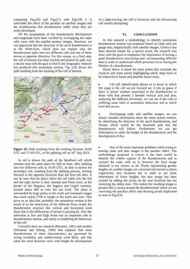
In order to see which is the main motion of the whole system, and if the assumptions of the cell development of the cells are correct, it has been plotted the cells at 16:24 UTC over the parallax corrected brightness temperature image (Fig.18). In this image, the parallax effect has been corrected by using the real Barcelona sounding of the 10th July 2013 at 12:00 UTC; unfortunately, at certain heights the sounding has temperature inversion (Fig.19), what makes the computation of the cloud height erroneous and, therefore, affecting the parallax correction.
Figure 18: Radar cells from the 3-D identification process at 1 km elevation, over the parallax corrected 9 channel brightness temperature image.
Figure 19: Barcelona sounding of the 10th July 2013 at 12:00 UTC with the inversion levels marked.
From the previous figures, it can be observed how the cell of interest (number 6 in Fig.17), is located on a region with maximum brightness temperature, what means that the cell is really developed to high levels, coinciding with the 3D identification methodology. It reaches cold temperatures as -55 ºC, as can be seen in Fig. (20), where it has been coloured the coldest regions of the cloud.
In any case, it results easy to associate the radar information to the MSG fields.
Figure 20: Radar cells from the 3-D identification process at 1 km elevation, over a coloured cloud top brightness temperature image of the 10th July 2013 at 16:24 UTC.
Figure 21: Radar cells from the 3-D identification process at 1 km elevation, over a coloured Overshooting Tops image of the 10th July 2013 at 16:24 UTC and zoom of cell 6.
Fig.(21) shows how cell 6 is located on a region where
we can find an Overshooting Top, because the coldest part of the thunderstorm is reaching the lower stratosphere, and reaching the height of at least 12 km. Furthermore,
Màster de Meteorologia 17 Universitat de Barcelona, Curs 2014-2015
comparing Fig.(20) and Fig.(21) with Fig.(18) it is noticeable the effect of the parallax on satellite images and the misallocation that thunderstorm suffer when they are really developed.
All the assumptions of the thunderstorm development and magnitude have been verified by overlapping the radar cells cores with the satellite product images. However, we can appreciate that the direction of the anvil thunderstorm is to the North-East, which does not explain why the thunderstorm splits into two different cells and one of these moves at opposite direction. For this reason, as a final step, the cell of interest has been tracked and plotted its path over a terrain map with the goal to find if any orographic obstacle has produced this anomalous motion. Fig. (22) shows the path resulting from the tracking of the cell of interest.
Figure 22: Path resulting from the tracking between 16:00 UTC and 17:30 UTC, of the splitting cell on 10th July 2013.
In red is shown the path of the “mother” cell which remains near the same place for half an hour, after splitting into two different cells at 16:30 UTC. In blue is shown the secondary cell, resulting from the splitting process, moving forward to the opposite direction than the first cell does. It can be seen that the place where the cell splits into the left and the right mover is near Sanaüja and Ponts town, at the border of the Noguera, the Segarra and Urgell counties, located about 400 m over the sea level. The place is surrounded by huge plains to the south and mountain ranges that reach nearly 1700 m height to the north and west. This gives us an idea that, probably, the anomalous motion is the result of an the interaction of the different flows inside the thunderstorm structure like vertical and horizontal wind shear due to the differences of terrain is passing by. Also the advection at low and high levels has an important role in thunderstorms motion, and surely is modelling the behaviour of the cell.
Currently there are research (Rotunno, 1981) and models (Weisman and Klemp, 1984) that explains that most thunderstorms of these characteristics are governed by strong instability and unidirectional wind shear, and that when the wind direction veers with height the development
of a right-moving, the cell is favoured with the left-moving cell usually dissipating.
VI. CONCLUSIONS
In this research a methodology to identify anomalous thunderstorm motion was proposed based on radar and rain gauge data, helped finally with satellite images. Unless it has been showed results for a special event, the research was done with the goal to emphasize the importance of having a good thunderstorm nowcasting tool, encompassing different data in order to understand which processes occur during the lifetime of a thunderstorm.
Down below is listed the main points that conclude the research and some points highlighting which steps have to be improved in future and possible future work.
• 3-D cell identification allows us to know in which life stage is the cell we are focused on; it lets us guess if there is severe weather associated to the thunderstorm in those cells that present a bended vertical axis and also, analysing the different elevations, we can see if the cells is suffering some kind of anomalous behaviour and at which level this occurs. • Overlapping radar and satellite images, we can obtain valuable information about the mean system motion, by identifying the direction of the anvil thunderstorm, and foresee which would be the “normal” path that the thunderstorm will follow. Furthermore we can get information to ratify the height of the thunderstorm and the development of this.
• One of the most important problems while trying to overlap radar and data images is the parallax effect. The methodology proposed to correct it has been useful to identify the coldest regions of the thunderstorms and to connect the radar cells on it, however the final image obtained is not correct at all. Pixels representing greater heights on satellite images are corrected and moved to theirs respectively new locations but in order to not loose information of lower heights, the new image has been created by adding the pixels on the new locations but not removing the oldest ones. This makes the resulting image to present like a corona around the thunderstorms which we are correcting the parallax effect and showing pixels duplicated as seen in Fig.(23).
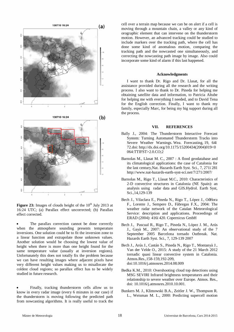
Màster de Meteorologia 18 Universitat de Barcelona, Curs 2014-2015
Figure 23: Images of clouds height of the 10th July 2013 at 16:24 UTC; (a) Parallax effect uncorrected; (b) Parallax effect corrected. • The parallax correction cannot be done correctly when the atmosphere sounding presents temperature inversions. One solution could be to fit the inversion zone to a linear function and extrapolate those unknown values. Another solution would be choosing the lowest value of height when there is more than one height found for the same temperature value (usually at inversion regions). Unfortunately this does not totally fix the problem because we can have resulting images where adjacent pixels have very different height values making us to misallocate the coldest cloud regions; so parallax effect has to be widely studied in future research.
• Finally, tracking thunderstorm cells allow us to know in every radar image (every 6 minutes in our case) if the thunderstorm is moving following the predicted path from nowcasting algorithms. It is really useful to track the
cell over a terrain map because we can be on alert if a cell is moving through a mountain chain, a valley or any kind of orographic element that can intervene on the thunderstorm motion. However, an advanced tracking could be studied to include markers over the tracking path, where the cell has done some kind of anomalous motion, comparing the tracking path and the nowcasted one simultaneously, and correcting the nowcasting path image by image. Also could incorporate some kind of alarm if this last happened.
Acknowledgments
I want to thank Dr. Rigo and Dr. Llasat, for all the assistance provided during all the research and the writing process. I also want to thank to Dr. Pineda for helping me obtaining satellite data and information, to Patricia Altube for helping me with everything I needed, and to David Tena for the English correction. Finally, I want to thank my family, especially Marc, for being my big support during all the process.
VII. REFERENCES
Bally J., 2004: The Thunderstorm Interactive Forecast System: Turning Automated Thunderstorm Tracks into Severe Weather Warnings. Wea. Forecasting, 19, 64–72.doi: http://dx.doi.org/10.1175/15200434(2004)019<0064:TTIFST>2.0.CO;2
Barnolas M., Llasat M. C., 2007 : A flood geodatabase and its climatological applications: the case of Catalonia for the last century,Nat. Hazards Earth Syst. Sci., 7, 271–281 http://www.nat-hazards-earth-syst-sci.net/7/271/2007/
Barnolas M., Rigo T., Llasat M.C., 2010: Characteristics of 2-D convective structures in Catalonia (NE Spain): an analysis using radar data and GIS.Hydrol. Earth Syst, Sci.,14,129-139
Bech J., Vilaclara E., Pineda N., Rigo T., López J., O’Hora F., Lorente J., Sempere D., Fàbregas F.X., 2004: The weather radar network of the Catalan Meteorological Service: description and applications. Proceedings of ERAD (2004): 416–420. Copernicus GmbH
Bech J., Pascual R., Rigo T., Pineda N., López J. M., Arús J., Gayà M., 2007: An observational study of the 7 September 2005 Barcelona tornado Outbreak. Nat. Hazards Earth Syst. Sci., 7, 129-139 2007
Bech J., Arús J., Castán S., Pineda N., Rigo T., Montanyà J., Van der Velde O., 2015: A study of the 21 March 2012 tornadic quasi linear convective system in Catalonia. Atmos.Res.,158-159,192-209, doi:10.1016/j.atmosres.2014.08.009
Bedka K.M., 2010: Overshooting cloud top detections using MSG SEVIRI Infrared brightness temperatures and their relationship to severe weather over Europe. Atmos. Res., doi: 10.1016/j.atmosres.2010.10.001.
Bunkers M. J., Klimowski B.A., Zeitler J. W., Thompson R. L., Weisman M. L., 2000: Predicting supercell motion
Màster de Meteorologia 19 Universitat de Barcelona, Curs 2014-2015
using a new hodograph technique. Wea. Forecasting, 15, 61–79.
Brunner J.C., Ackerman S.A., Bachmeier A.S., Rabin R.M., 2007:A quantitative analysis of the enhanced-V feature in relation to severe weather. Wea. Forecasting 22, 853–872.
Carretero O., Martín F., Elizaga F., 2001: Radar-based perspective of different convection episodes in the western Mediterranean areas. Mediterranean Storms, Proceedings of the 3rd EGS Plinius Conference held at Baja Sardinia, Italy, October 2001
Cavcar, M., 2000: The International Standard Atmosphere (ISA). Anadolu University, 26470.
Doswell C.A. III., Brooks H.E., Maddox R-A., 1996: Flash Flood Forecasting: An Ingredients-Based Methodology Wea. Forecasting, 11, 560-581
Doswell C.A. III, 2001: Severe convective storms – An overview. Severe Convective Storms, Meteor. Monogr., 28, n. 50, Amer. Meteor. Soc., 1-26
Farnell C., Busto M., Aran M., Andres M., Pineda N., Torà M., 2009: Estudi de la pedregada del 17 de setembre de 2007 al Pla d’Urgell. Primera part: treball de camp i anàlisi dels granímetres (in Catalan). Tethys, 6, 69–81 doi:10.3369/tethys.2009.6.05
Feral L., Mesnard F., Sauvageot H., Castanet L., Lemorton J., 2000: Rain cells shape and orientation distribution in South-West of France, Phys. Chem. Earth Pt. B, 25(10–12), 1073–1078
Fujita T., Grandoso H., 1968: Split of a thunderstorm into anticyclonic and cyclonic storms and their motion as determined from numerical model experiments. J. Atmos. Sci., 25, 416–439.
Gayà M., Llasat Botija M. D. C., Arús Dumenjó J., 2011: Tornadoes and waterspouts in Catalonia (1950-2009). Natural Hazards and Earth System Sciences, 2011, Vol. 11, p. 1875-1883.
Goodrich D.C., Faurès J.M., Woolhiser D.A., Lane L.J. Sorooshian S., 1995. Measurement and analysis of small-scale convective storm rainfall variability. Journal of Hydrology, 173 (1–4), 283–308. doi: 10.1016/0022-1694(95)02703-R
IGC, 2013: Informe preliminar dels efectes dels aiguats i riuada del 18 de juny de 2013 a la conca de la Garona. Institut Geològic de Catalunya, Generalitat de Catalunya, 81 pp.
Jansa A., Alpert P., Arbogast P., Buzzi A., Ivancan-Picek B., Kotroni V., Llasat M.C., Ramis C., Richard E., Romero R., Speranza A., 2014: MEDEX: a general overview Nat. Hazards Earth Syst. Sci., 14, 1965–1984 http://www.nat-hazards-earth-syst-sci.net/14/1965/2014/
Johnson J.T., MacKeen P.L., Witt A., Mitchell E.D., Stumpf G.J., Eilts M-D., Thomas K.W., 1998: The storm Cell Identification and Tracking (SCIT) Algorithm: An Enhanced WSR-88D Algorithm. Weather and Forecasting. June1998, vol. 13, pp 263-276
Koenig, M., de Coning, E., 2009: The MSG global instability indices product and its use as a nowcasting tool. Weather and forecasting, 24(1), 272-285
Llasat M.C., 2001: An objective classification of rainfall events on the basis of their convective features. Application to rainfall intensity in the NE of Spain. Int. J. Climatol., 21, 1385-1400.
Llasat M.D.C., Rigo T., Barriendos M., 2003: The ‘Montserrat‐2000’ flash‐flood event: a comparison with the floods that have occurred in the northeastern Iberian Peninsula since the 14th century. International Journal of Climatology, 23(4), 453-469.
Llasat M.C., Barriendos M., Barrera A., Rigo T., 2005: Floods in Catalonia (NE Spain) since the 14th century. Climatological and meteorological aspects from historical documentary sources and old instrumental records. Journal of Hydrology, 313(1), 32-47.
Llasat M.C., Ceperuelo M., Rigo T., 2007: Rainfall regionalization on the basis of the precipitation convective features using a raingauge network and weather radar observations. Atmospheric research 83.2 :415-426.
Machado L.A.T., Lima W.F.A., Pinto O., Morales C.A., 2009: Relationship between cloud-to-ground discharge and penetrative clouds: a multi-channel satellite application. Atmos. Res. 93, 304–309.
Martín F., Elizaga F., Carretero O., San Ambrosio I., 2007: Diagnóstico y predicción de la convección profunda (in Spanish). Technical Note n. 35 of the Analysis and Forecasting Technical Service of the Spanish Weather Service, 174 pp.
Mecikalski, J. R., Bedka, K. M., 2006: Forecasting convective initiation by monitoring the evolution of moving cumulus in daytime GOES imagery. Monthly Weather Review, 134(1), 49-78.
Morel, C., Sénési, S., Autones, F., 2002 : Building upon SAF-NWC products: Use of the Rapid Developing Thunderstorms (RDT) product in Météo-France nowcasting tools. In Proc. The (pp. 248-255).
Northrop P.J., 1998: A clustered spatial-temporal model of rainfall, P. Roy. Soc. Lond., A454, 1875–1888
Parker M.D., Johnson R.H., 2000: Organizational modes of midlatitude mesoscale convective systems. Monthly weather review 128, 10, 3413-3436
Pineda N., Soler X., Vilaclara E., 2011: Aproximació a la climatologia de llamps a Catalunya: anàlisi de les dades de l’SMC per al període 2004-2008 (in Catalan). Tech. Note n. 73 of the SMC, 71 pp
R Core Team, 2013: R: A Language and Environment for Statistical. R Foundation for Statistical Computing. Vienna, Austria
Radová M., Jakub S., 2008: Parallax applications when comparing radar and satellite data. The 2008 EUMETSAT Meteorological Satellite Conference.(this conference proceedings).
Màster de Meteorologia 20 Universitat de Barcelona, Curs 2014-2015
Reynolds, D.W., 1980. Observations of damaging hailstorms from geosyn-chronous satellite digital data. Mon. Wea. Rev. 108, 337–348.
Rigo T., Llasat M.C., 2002: Analysis of convection in events
with high amounts of precipitation using the meteorological RADAR. In: Proceedings of the 4th EGS Plinius Conference on Mediterranean Storms, edited by: Jansa, A. and Romero, R., Mallorca, Spain. p. 2-4.
Rigo T., Llasat M.C., 2004: A methodology for the
classification of convective structures using meteorological radar: Application to heavy rainfall events on the Mediterranean coast of the Iberian Peninsula. Nat. Hazards Earth Syst. Sci., 4 (1), 59-68
Rigo T., Llasat M. C., 2007: Analysis of mesoscale
convective systems in Catalonia using meteorological radar for the period 1996–2000, Atmos. Res., 83, 458–472
Rigo T., Pineda N., Bech J., 2008: Estudi i modelització del
cicle de vida de les tempestes amb tècniques de teledetecció (in Catalan). Tech. Note n. 72 of the SMC, 58 pp
Rigo T., Serra A., Berenguer Ferrer M., 2013: Integració de
dades de radar i pluviòmetre per a la predicció meteorològica d'avingudes.
Rosenfeld D.,Lensky I., Kerkmann J., Tjemkes S., Govaerts
Y., Roesli HP., 2004: Conversion from counts to radiances and from radiances to brightness temperature and reflectances. Oral presentation in “Applications of Meteosat Second Generation (MSG). A MSG Interpretation Guide”. EUTMETSAT, 2004
Rotunno, Richard, 1981: On the evolution of thunderstorm
rotation. Monthly Weather Review 109. 577-586.
Schmetz J., Tjemkes S. A., Gube M., Van de Berg L., 1997: Monitoring deep convection and convective overshooting with METEOSAT. Advances in Space Research, 19(3), 433-441.
Schmetz J., Pili P., Tjemkes S., Just D., Kerkmann J., Rota S., Ratier A., 2002: An introduction to Meteosat second generation (MSG). Bulletin of the American Meteorological Society, 83(7), 977-992.
Schmetz J., Pili P., Tjemkes S., Just D., Kerkmann J., Rota S., Ratier A., 2002: SEVIRI calibration. Bull. Am. Meteorol. Soc, 83.
Tapia A., Smith J.A., Dixon M., 1998. Estimation of convective rainfall from lightning observations, J. Appl. Meteorol. 37(11), 1497 – 1509.
Velasco-Forero C. A., Sempere-Torres D., Cassiraga E. F., Gómez-Hernández J. J., 2009: A non-parametric automatic blending methodology to estimate rainfall fields from rain gauge and radar data. Advances in Water Resources, 32(7), 986-1002.
Weisman, Morris L., Klemp, Joseph B., 1984: The structure and classification of numerically simulated convective storms in directionally varying wind shears. Monthly Weather Review 112.12: 479-2498.
Wilhemson R.B., 1974: The life cicle of a thunderstorm in three dimensions. J. Atmos. Sci., 31,1629-1651
Wolf R., Just D., 1999: LRIT/HRIT global specification. Coordination Group for Meteorological Satellites, (2.6).