icl technical journal volume 2 issue 3 - may 1981 board welcomes mr. davies with this issue of the...

TechnicalJournal

Volume 2 Issue 3 May 1981

ICL TechnicalJournal

ContentsVolume 2 Issue 3

A dynamic database for econometric modellingT.J. Walters 223

Personnel on CAFS: a case studyJ. W.S. Carmichael 244

Giving the computer a voiceM.J. Underwood 253

Data integrity and the implications for back-upK. H.Macdonald 271

Applications of the ICL Distributed Array Processor in econometric computations

J.D.Sylwestrowicz 280A high level logic design system

M.J. Y. Williams and R. W.McGuffin 287Measures of programming complexity

Barbara A.Kitchenham 298

Editorial Board

Professor Wilkes retired from his Chair at Cambridge in the autumn of 1980 and is now living in America; he has decided to resign from the Editorial Board, on grounds of practicality. The Board and the management of ICL take this opportunity to record their very warm appreciation of the great amount he has done for the Technical Journal. His wisdom and his advice, based on his unrivalled experience as one of the pioneers of the computer age, and his insistence as a scientist and a scholar on high but realistic standards have been invaluable. The Board sends its thanks and good wishes to a colleague who is greatly respected and whose company has always been enjoyed.

It is the Board’s good fortune that Mr. Donald Davies of the National Physical Laboratory has accepted the Company’s invitation to become a member. He too has experience going back to the earliest days of the digital computer, for whilst Professor Wilkes was building one classic machine, EDSAC, at Cambridge, he was one of the team which was building another, ACE, at NPL. The Board welcomes Mr. Davies with this issue of the Journal.

ICL TECHNICAL JOURNAL MAY 1981 221

ICL TechnicalJournal

The ICL Technical Journal is published twice a year by Peter Peregrinus Limited on behalf of International Computers Limited

EditorJ.HowlettICL House, Putney, London SW15 1SW, England

Editorial Board J. Howlett (Editor)D.W.Davies(National Physical Laboratory)D.P Jenkins(Royal Signals & Radar Establishment) C.H.Devonald

D. W. Kilby K.H. Macdonald B.M. Murphy J.M. PinkertonE. C.P. Portman

All correspondence and papers to be considered for publication should be addressed to the Editor

Annual subscription rate: £10 (cheques should be made out to ‘Peter Peregrinus Ltd.’, and sent to Peter Peregrinus Ltd., Station House, Nightingale Road, Hitchin, Herts, SG5 1RJ, England. Telephone: Hitchin 53331 (s.t.d. 0462 53331).

The views expressed in the papers are those of the authors and do not necessarily represent ICL policy

PublisherPeter Peregrinus LimitedPO Box 8 , Southgate House, Stevenage, Herts SGI 1HQ, England

This publication is copyright under the Berne Convention and the International Copyright Convention. All rights reserved. Apart from any copying under the UK Copyright Act 1956, part 1, section 7, whereby a single copy of an article may be supplied, under certain conditions, for the purposes of research or private study, by a library of a class prescribed by the UK Board of Trade Regulations (Statutory Instruments 1957, No. 868), no part of this publication may be reproduced, stored in a retrieval system or transmitted in any form or by any means without the prior permission of the copyright owners. Permission is however, not required to copy abstracts of papers or articles on condition that a full reference to the source is shown. Multiple copying of the contents of the publication without permission is always illegal.

©1981 International Computers Ltd

Printed by A.McLay & Co. Ltd., London and Cardiff ISSN 0142-1557

222 ICL TECHNICAL JOURNAL MAY 1981

Adynamic database for econometric modelling

T.J.WaltersICL European Division, Putney, London

Abstract

Many countries, especially those in the Third World and COMECON groups, have government agencies responsible for macro-economic planning. These agencies maintain large econometric databases covering national and international economic statistics. The paper describes an integrated system which has been designed to enable such organisations, who may not have any specialist computer knowledge, to construct, evaluate and tune econometric models. Particular attention is paid to the needs for storage, cataloguing, identification and retrieval of data and the facilities provided are based on the ICL Data Dictionary System. Examples are given of typical dialogues which might take place between a user and the system.

1 Introduction

The system which forms the subject of this paper is the result of a feasibility study made on behalf of a State Planning Committee for a new system to be implemented in 1982-83; it looks forward also to the likely development of the system beyond that date. The bulk of the work of the Committee is the formulation of national macro-economic plans with time-frames of 1, 5 and 15 years which, when they have been agreed, must be monitored in operation to enable corrective measures to be taken if economic performance starts to deviate from the plan. Plans are based on models of national and international economies and optimisation is done by Linear Programming (LP) techniques: indeed, LP was developed specifically in the USSR in the 1920s for this purpose and a wealth of experience in such modelling has been amassed by mathematicians and economists world-wide over the years.1

The impact on this work of the ‘information explosion’ has only recently begun to be felt. In the organisation on which this study was based there is at present a library of economic statistics containing about 3x l09 bytes of data, largely organised into about 60 000 ad hoc matrices which have been built up over the last 15 years. In spite of a decision to discard data relating to periods of over 20 years in the past, this library is expected to exceed 1010 bytes within the next 10 years. This growth comes mainly from two sources: externally in the form of new (‘raw’) data provided by various outside bodies such as the country’s Department of Trade or the Census Bureau, internally through the generation of new statistics and analyses as a by-product of users’ processing of existing data. Merely to maintain the catalogue of such a volume of data is itself a major task and in this case the problem is


compounded because different users may take radically different views of the same aspect of the economy and of the data relating to it, and there is a need for the catalogue to reflect these varying points of view. At present the catalogue is held manually in the computer centre, whose staff are involved in assisting the econometricians in constructing their models. It is felt that as the demands grow this will place too great a burden on the computer centre staff and that a new method of procedure must be found, taking advantage of the developments in decentralised computing. The outcome of the study has been that a new system has been proposed, aimed at enabling econometricians to interact directly with the computer through a terminal, the system providing them with the guidance previously provided by the computer centre staff on what data is available, what suitable processing techniques there are and how to use these.

Since users of the system will, as a by-product of their work, be generating data which may be relevant to other users at some later date, and since it is not feasible to impose a discipline on this when it is actually happening, we must design a self- documenting database which will assume many of the functions traditionally performed manually by the Data Administrator. This type of requirement arises in other contexts than econometric modelling and the problems which it presents are being tackled as a logical extension o f recent work on data dictionaries.2

Typically an econometrician takes several weeks to construct and tune a model, running and refining it repeatedly until it is well behaved and he is satisfied that it is a satisfactory representation of reality. During this process he will make regular use of a MAC terminal to tune and try out his model, just as any programmer might when developing a program. In the new system he has two distinct methods of identifying the data he wishes to process. If he has used this recently, as will often be the case because he will tend to develop one model over several months, he may be able to identify it by a previously-allocated name and so enable the system to retrieve it directly. But when he starts to construct a model he may not know of any identity for the data he wants; indeed he may not know what relevant data there is or whether any exists at all. He then needs to locate any data related to his problem, with enough descriptive information to enable him to decide whether any is suitable, or can be made suitable, for his purposes. The system must allow him to express his needs in terms which are familiar to him.

The system which has been developed does provide such a service, and also enables a user to specify directly the processing he wishes to perform, if he knows this, and how to specify it. Otherwise the system enters into a dialogue with him and discusses his requirements interactively until it has established what processing is to be done; it then tells the user the direct way of specifying these processes and performs them. This is illustrated in Appendix 1. In many cases only the requirements for data and processing are established interactively, the system then setting up a batch job to extract and process the data. This is so if the data is not on-line or if the processing is mill-intensive. Only about 10% of data is held on-line at any time, although this is expected to represent over 80% of data accesses.


2 How the user sees his data

As mentioned above, there is considerable disparity between the ways different econometricians, modelling different areas of the economy, see the same data. However, most see their data as occupying positions within a space which can be conceived of as having several dimensions or ‘axes’. There is considerable agreement between different econometricians’ concepts about what the main axes are, the four most generally visible being:

TimeGeography Product/product type Economic unit/grouping.

This does not mean that all users use all of these, nor that they use only these, nor even that where they use the same axis they agree about its structure. But these four standard axes do form a lowest common denominator to which all users can relate easily even when disagreeing about details. Another point of agreement is that the axes are organised hierarchically; for example, some users considering foreign trade will see the geography axis as

the world made up of continents made up of countries.

metastructure

world

Acontinent

Acountry

structure

Fig. 1 Hierarchical structures

This view may be represented schematically as in Fig. 1. The left-hand diagram represents the metastructure, with the crow’s-foot symbol showing a one-to-many relationship between the elements. The right-hand diagram, which for space reasons


is obviously incomplete, shows the actual structure. Other users may group countries by trading block and see the following structure

the world made up of trading blocks made up of countries.

These two classifications overlap and, as in many cases, have elements in common at the lowest level; here because both users mean the same thing by ‘country’. The relationship between the two structures is shown in Fig. 2. The overlap and commonality have important benefits in that they make it possible for data structured to one user’s view to be accessed meaningfully by another user. In this example the ‘raw’ data would be by country and the system would summarise it by continent or by trading block as appropriate.

metastructure

structure

Fig. 2 Overlapping structures


Other users group countries in yet further ways, for example by GNP per head of population, or according to major imports or exports, and all these alternative structures can be superimposed. In the example above there is also commonality at the highest level since ‘the world’ in both cases covers all countries. This however is not always the case since some users wish to consider only certain countries and ignore the rest: someone studying energy production may wish to consider only countries which export coal, gas and petroleum for example. In this case there is still commonality at the lowest level, although one user sees only a subset of the other’s countries, but none at the top.

Still other users see a very different geographical axis, especially if they are modelling the internal economy. They see the country at the highest level, divided into counties, towns etc, with various alternative groupings of the same lowest level units. It is conceivable that some econometricians analysing imports or exports by county will want actually to have two geographic axes, one domestic and one international. A case can be made for regarding these as two distinct standard axes and it is possible that this maybe done in the future. The system is deliberately designed to be evolutionary and thus allows changes to the standard axes.

Other axes may have similar hierarchical structures; for example, in the case studied here the time axis is divided into 5 year, 1 year, quarter and month periods. There is no 15-year unit because the 15-year plan is a ‘rolling’ one, meaning that at any instant the current 15-year plan is composed of the current 5-year plan followed by its two successors. At the other end of the scale, whilst the shortest term plan is for 1 year, modelling for this is done on a finer time scale and much raw data is on a quarterly or monthly basis. The time axis is not expected to have alternative hierarchies, although some users will use only a subset of the standard; but in the interests of homogeneity the system treats all axes identically, so the potential for alternatives exists.

Alternative structures are particularly prevalent on the remaining standard axes, Product and Economic Unit. There are many different ways of grouping products together and since the construction of economic models involves considerable skill and judgement there could be as many structures as models. However in practice human nature comes to the rescue: defining these structures is laborious and boring, so there is a tendency for a worker to use the same structure as for his last model or to ‘borrow’ a structure from a colleague. It could be argued that the system, in the interests of facilitating the construction of accurate models, should make it easy for users to define new structures but in practice there are good reasons for not doing so. First, there is no simple way of providing an effortless means for defining structures; second, minor deviations from the ideal do not have any significant effect on the accuracy of the model; and third, an undue proliferation of alternative structures will produce an unnecessary overhead, particularly of disc storage.

Similarly there are many ways of grouping firms, for example by type of business, by location, by size (number of employees, turnover etc.) or by economic sector, e.g. public or private.


Apart from standard axes, users can also see other structures. For example, a user modelling economic performance in some industry is interested in the income, expenditure, profits, labour costs, capital investment etc. of firms and may see this as having a structure. Fig. 3 illustrates this. In this example the structure reflects mathematical relationships as well as logical ones. In other cases only the logical relationship may be present; thus if ‘number of employees’ is added to the above example there is the non-mathematical relationship between number of employees and labour costs.

Fig. 3 Possible financial structure for an industry

2.1 Representing user-seen structures

The ICL Data Dictionary System (DDS)3 provides a suitable vehicle for representing these structures. The Data Dictionary is partitioned into four main areas or quadrants, as shown in Fig. 4. The user-seen structures are recorded in the ‘Conceptual Data’ quadrant which records entities, attributes and relations between entities as shown in Fig. 5 . As we shall see later, the actual data can be represented in the ‘Computer Data’ quadrant and the conceptual data mapped on to it.

The standard approach is to use the ‘Conceptual Data’ quadrant of the DDS to record metastructures and to hold the actual hierarchies elsewhere, for example in an IDMS database, and this is well suited to a conventional data-processing environment where the metastructure can be defined in a (relatively) static schema4 In such an environment, where changes to the schema are infrequent and are controlled by the data administrator4 , this causes no difficulty; but in the present system where users can create new hierarchies at will it imposes an unacceptable restriction. The DDS,on the other hand, is designed to be dynamic and it allows new elements and structures to be defined at any time and is therefore a much more suitable vehicle for defining the user-seen hierarchies.


Fig. 4 Data Dictionary Quadrants

In defining these hierarchies we must decide whether the elements are entities or attributes — a question frequently debated by data lexicographers with the same fervour as in mediaeval theologians’ disputations over the Trinity or as physicists once argued over particles and waves. The distinction between an entity and an attribute becomes very difficult to maintain in an environment where users often take radically different views of the same data, so we have embraced the precedents of the theologians and the physicists and fudged the issue by adopting the convention that every element is simultaneously an entity and an attribute.

3 How data is held

The most common structures are tables, matrices and data matrices; others such as arrays, scalars and lists are also required. For the present purposes we shall consider only the first three; they are the most interesting and once they have been dealt with the representation of the others is a trivial problem.


Fig. 5 Conceptual Data Quadrant

3.1 Data matrix

This is a rectangular array of data in rows and columns in which the rows are called cases and the columns variates. It normally contains raw data such as is obtained from a survey or a census. For a census a case would represent a person and a variate the answers by all persons to one question. One important characteristic of a data matrix is the fact that variates can be of different types: real and integer are most common but other types such as character, logical and name are often required. Most statistical systems treat the data matrix as a serial file with one record for each case, reflecting the normal means of processing case by case. It is rare for it to be either necessary or possible to hold the complete matrix in main store; data matrices can usually be stored as serial files.

In computer terms, data matrices are held as a sequence of data records, each corresponding to one row or case and containing a series of items which are the variates


for this case. In addition each matrix has three header records which act as identifiers: one for the data matrix as a whole, a column header record containing a series of column headers or variate identifiers and a row header record containing a series of row headers or case identifiers. These case and variate identifiers correspond to entities/attributes at the conceputal level. For example, a data matrix of company results would have column headers corresponding to the elements of the structure shown in Fig. 3 and the row headers would be the case identifiers relating to individual firms represented on the hierarchy of the Economic Unit axis. We shall examine later how we record these correspondences, as well as other relationships between the data matrix and the user’s view such as the year to which the data relates (time axis) and the fact that it relates to all products and the whole country (product and geography axis).

3.2 Table

This may have any number of dimensions although two is the most common. Tables of more than two dimensions can be treated as a sequence of two-dimensional tables. The entries must be all of the same type; they are often frequencies and therefore of type integer but they could be of other types, for example the numerical values of a variate. Most statistical systems which recognise the table as a data structure retain as part of the table some descriptive information on how the cells were formed: that is, the boundaries, ranges, levels etc. which define the cells are retained for each dimension. Tables with just two dimensions are frequently held in main store, particularly when access to individual entries is required; thus there is usually a main-store form as well as an external backing-store form for a table.

Tables are held externally in backing store in a way similar to data matrices, that is, as a sequence of data records corresponding to individual rows; and in main store as an n-dimensional matrix. In addition, as with data matrices, each table has a series of header records: a table header record followed by an axis header record for each dimension, where each axis header contains a series of vector header items identifying that row or column. The vector headers may correspond to entities/attributes at the conceptual level, but not necessarily so; for example, if a table contains frequency distributions the vector headers for one or more axes will contain boundaries, limits of ranges which do not correspond to user-seen entities.

3.3 Matrix

This is the usual rectangular arrangement of values, all of the same type. Values are usually o f type real or integer but again other types such as boolean are possible. The matrix may frequently be held in main store with operations on individual elements allowed. The internal representation is usually as a normal computing- language array with two dimensions, and a number of arrangements on external magnetic media is possible. The matrix is often formed from a data matrix, a table or other matrices and does not often contain raw data. Among many possibilities it may contain frequencies obtained from one or more tables or values such as correlations derived from a data matrix.


Matrices are held as a special case of tables, with only two dimensions.

3.4 Recording data structures

We can generalise these data structures as shown in Fig. 6 where ‘Matrix’ is used as a general term for Table, Matrix or Data matrix. Some of the relations are many-to- many because the same vector may occur in different axes (of different matrices) and it is even possible for different matrices to have a complete axis in common — as, for example, when one matrix is a by-product of processing another.

Fig. 6 Metastructure of data

The ICL DDS does not recognise Matrix, Axis or Vector as element types but does recognise File, Record and Item which have the required relationships and which we can use in their place. These are shown in Fig. 7. This use of the elements is unorthodox but not unreasonable, since in fact each matrix is held in the VME/B filestore as a file and, as explained above, we wish to hold a record for each axis containing an item for each vector. What is more unconventional is that the Record element is meant to refer to a record type, whereas we have one for each axis although the axis records are, strictly speaking, all of the same type. Similarly we have an Item element for each vector although they are repeated items of the same type. In fact, just as in the Conceptual Data quadrant, we are using the Data Dictionary to hold the data of these axes records and not just their description. The reason we do this is that the data, in particular the vector identifiers, relate to elements in the Conceptual Data quadrant and we can use the DDS’s mapping mechanisms to record these links, as shown in Fig. 8. Because we are holding the axis data in the Data Dictionary we do not need to hold it again in the data file, so this latter is reduced to holding only the data records.


4 How the user processes the data

4.1 Finding the data

Now that we have described the structures of the Conceptual Data and Computer Data quadrants of the data file we can trace the paths used by the system in helping the user to identify his data and to locate this for him.

To start with, a user will name a variable which he wishes to process and the system will search for an entity with this name. If it cannot find one it will ask him for alternative names or names of related variables until it has found the variable he wants. It will confirm this by displaying the structure of which this entity is part ; if this structure is too large to display conveniently it will display the other entities most closely related to the one in question. If no suitable entity can be found this phase is abandoned and the system proceeds to the next stage.

Fig. 7 Computer Data Quadrant


Fig. 8 DDS mapping of Conceptual and Computer Data

Next the system asks how the user wants to analyse his variable, offering analyses by each of the standard axes. If the user asks for any of these he is asked what structure he wants to use, being prompted with standard structures for this axis plus any special ones he may have defined in the past. If none of these is suitable he is asked to define the structure he requires. Once the system has located these structures in the Conceptual Data quadrant it uses the links to the Computer Data quadrant to find any matrices, tables etc. linked to the structures he wishes to use as analysis criteria, and to the variables he is interested in. If the system cannot find any suitable data it identifies data linked to related entities and offers this, suggesting ways it can be manipulated to make it fit the user’s specification. Finally the system enquires what other variables the user is interested in and whether he wants these classified in the same way, and locates suitable data. When the user has identified all his data the system tells him the quick way to specify it for him to use the next time he wants it and goes on to enquire what processing he requires.


An example of such an interactive session is given in Appendix 1.

This navigation of the Data Dictionary is possible because

(a) all elements have, in IDMS terms, CALC keys containing two sub-keys, element type and element name

(b) the linkages shown in Fig. 8 are all recorded.

Furthermore, all elements have an ‘owner’ who is the user who created them; this does not necessarily preclude others from accessing them but it does enable the system to distinguish one user’s axis structures from another’s.

The processing requirements also can be determined interactively if the user is not sure how to specify them; this is done with the aid of a development of the ICL Package-X statistical system.5

4.2 Specifying the processing requirements

Package X enables the planner to approach the system from three positions.

He may know - the program he requires— the analysis he requires but not the program— neither the analysis nor the program.

The information necessary to identify the program for the planner from these starting positions can be organised in an IDMS database with the structure shown in Fig. 9. We consider the three possibilities.

(i) If the planner knows the name of the program this can be CALC computation on the PROGRAM record type.

(ii) If he knows the analysis but not the program, the appropriate ANALYSIS record may be located by CALC computation. From this the program or programs that provide the analysis can be located via the ANALYSIS IN PROGRAM record or records.

(iii) If he wishes to explore what is available for a particular problem he will enter an appropriate economic term which if necessary will be converted by the system into a standard term. Access can then be gained to a description of the term in the TERM DESCRIBE and to the appropriate analyses. Since many analyses may be appropriate, and one analysis may be relevant to many standard terms, access to ANALYSIS records can be made via the TERM IN ANALYSIS records. Having located the required program, the user may choose to select the dialogue which will allow him to specify what he wants the program to do for him. For this, the control program must first determine from the user which of the three starting positions applies. If (i), then access to the appropriate dialogue is direct. If(ii), the control must identify a possible program or programs. If there is


only one then access is again direct; if there are several then the user must be asked to choose which one he wants and this may require display of information about each of the possible programs.

These possibilities, and the way in which the system deals with them, are illustrated in the example given in Appendix 1. 5

Fig. 9

5 Setting up and maintaining the dictionary

One of the major attractions of the structure described is the ease of both creation and maintenance of the dictionary. Once standard structures have been defined for each of the standard axes — a relatively trivial task — work can begin on inputting the matrices contained in the present library. This involves only a small amount of human intervention for each one, giving the matrix identity, input format (the present system uses half-a-dozen standard formats corresponding to various application packages in use) and the user to whom the data belongs. This last is not to restrict access but to assist in linking the vectors to any user-defined structure in the Conceptual Data quadrant. If a matrix has vectors which do not correspond to any previously defined entity/attribute in the conceptual data then an attempt to create a link will not fail; instead the DDS will create a skeleton entry for the missing element and continue processing. This will normally occur when a user’s


data is input before he has defined the appropriate non-standard structures. Subsequently the DDS can output for each user a prompt list of all such unsatisfied cross-references, inviting him to define the missing elements.

Matrices generated during processing can be accommodated even more easily because the format is standard and the user is known, so all that remains to be done is to supply an identifier, which the user must do for the relevant application package anyway.

6 Implementation

The full implementation of such a system is likely to take many years; this paper has described only the direction of the first phase. The final specification — if an evolutionary system can be said to have a final specification — will emerge from the experience gained with the earlier stages, but the broad aim is clear: to make the user more self-sufficient and to lessen his dependence on other staff. Meanwhile, to enable a basic package to be developed quickly so that users may start to reap benefits before the development costs have risen too high, we have chosen to use as many existing products as possible, in particular Package-X and the DDS. The architecture of Package-X is such that it can be readily extended to encompass further processing routines, and even data retrieval routines, by expanding its database of programs and dialogues. The DDS provides a proven package for building and maintaining a data dictionary with facilities for amending and interrogating this and for ensuring integrity, security and resilience.

6.1 Adapting the DDS

There are some 15 standard interrogations supported by the DDS, of which the most common are:

(a) to find a particular instance of an element type: e.g. FIND ENTITY GROSS-PROFIT

(b) to find all elements of a given type linked directly to a named element: FOR RECORD SETTLEMENT AXIS FIND ALL ITEMS*

(c) to find all elements of a given type which are indirectly linked to a named element, the type of indirection being indicated:FOR ENTITY GROSS-PROFIT VIA ATTRIBUTES VIA ITEMS VIA RECORDS FIND ALL FILES

(d) to find all elements of all types which refer to a given element:FIND USAGE OF ATTRIBUTE GROSS-PROFIT.

*The term SETTLEMENT, here and later, is used to denote some geographical entity such as a town, a district etc.


More refinements of these interrogations are possible by further qualifying the elements to be searched. For example, as mentioned in Section 4, each element is ‘owned’ by a user and searching can be restricted to elements belonging to a particular user, not necessarily the current one. Elements can also be assigned to user-defined classes and only elements of particular classes retrieved. Any element can belong to several classes, up to a maximum of five, so that overlapping classifications are possible. These facilities are used, for example, in user-defined hierarchies where the ‘owner’ is the user who defined the hierarchy and the entities belong to classes which indicate whether they represent a metastructure or a structure, whether or not they are the root of this structure (or metastructure) and which axis they describe. This makes it easy to retrieve, say, all the geographical structures for a particular user in order to ask him which one he wishes to use.

Fig. 10 Metastructure of a tailor-made dictionary

While these interrogations provide some useful functions they do not operate on the terms or on the level which the user sees; it is therefore necessary to package them to present a more suitable user interface. There are two main ways of doing this.


The first is for the routines supporting the extended Package-X interface to call some of the routines from the standard enquiry program; this will be adopted in the first instance as it is a way of providing the interaction which is cheap and simple even though not always the most efficient. The second, which will be done later, is to write a purpose-designed program to support the required interrogations, using the formal DDS interface which enables COBOL programs to read the Data Dictionary. It would of course be possible to incorporate some of the routines from the standard enquiry program into this purpose-built software, to reduce the work involved, either as a temporary or a permanent measure.

6.2 Subsequent developments

As the data volumes and numbers of users increase it may become desirable to structure the dictionary differently so as to reduce the number of elements needed to describe the data and the user’s view and to reduce the number of linkages used to connect them. In that case a totally purpose-built system could be constructed using IDMS, analogous to the standard DDS but employing the elements and relations which are particular to the data in question. An example of how such a tailored dictionary might look is given in Fig. 10. This has four sections instead of the two in the standard DDS, representing conceptual metastructure, conceptual structure, actual metastructure and actual structure. As can be seen, this arrangement has no many-to-many relationships and therefore can be implemented in IDMS. An order of magnitude estimate for implementing such a tailor-made system, including archiving, recovery, maintenance and interrogation facilities is 20 man- years. In view of the steadily rising cost of custom-built software and the falling cost of hardware it is the author’s belief that it will always be more cost-effective to provide a more powerful hardware engine than to embark on a software project of this magnitude.

Acknowledgments

The author wishes to thank the following for their contributions to and comments on the system described in the paper: C.Clayman and B.E.Cooper, ICL Dataskil; AJones, ICL Sweden, and J.Watters, ICL European Division, Putney.

References

1 AUGUSZTINOVICS, M.: Application o f mathematical models and computers in longterm planning - a methodological summary, NPD, Budapest, 1977.

2 JONES, M.T. and SANKEY, T.: The MIAS oceanographic database: an integrated database/Data Dictionary in Database achievements, British Computer Society, London, 1979.

3 BOURNE, T.J.: The data dictionary system in analysis and design, ICL Tech. J. 1979, 1(3), 292.

4 IDMS technical overview, ICL Publication P1307, 1980.5 COOPER, B.E.: Statistical and related systems, ICL Tech. J. 1979, 1(3), 229.


Appendix 1

Example of dialogue between a user and the system

A .l Dialogue to identify data

System: What variable are you interested in?

User: PROFIT

What is profit an aspect of?

HELP

Do not recognise the variable profit Do you sometimes use another term for it?

GROSS PROFIT

I have a group of variables called COMPANY ACCOUNT: it is:

Total income Gross Profit

Net Profit Taxes

Total Expenditure Capital Expenditure Running Expenditure

Material Costs Wages Costs Overheads

Is this the GROSS PROFIT you mean?

YES

How do you want to analyse GROSS PROFIT?

HELP

Do you want to analyse by time?

NO

Do you want any particular time?

1978

Do you want to analyse by geography?

YES

The standard geographical analysis is:

Country containing:County containing:

District containing:Settlement

The last geographical analysis you used was ECONGEOG:

Country containing:Region containing:

Settlement size group containing: Settlement

Is one of these suitable?

ECONGEOG

By which units of ECONGEOG do you want to analyse?

SETTLEMENT SIZE GROUP

Do you want to analyse by industry?

NO

Do you want any particular industry?

NO

Do you want all industries?

YES

All industry is called “TOTAL ECONOMY” Do you want to analyse by product?

TOTAL PRODUCTS

I do not have a product structure called “TOTAL PRODUCTS”Do you want to analyse by product?

YES

Do you want any particular product(s)?

TOTAL PRODUCTS

Do you want to analyse by any othercriteria?

NO

I have no analysis of GROSS PROFIT by SETTLEMENT SIZE GROUP for 1978 for TOTAL ECONOMY for TOTAL PRODUCTS.I have an analysis of GROSS PROFIT by SETTLEMENT for 1978 for TOTAL


ECONOMY for TOTAL PRODUCTS. This is called 1978 COMPANY RESULTS BY

ALGORITHM = AGGREGATE)

SETTLEMENT. Can 1 use it?

YES

How should I derive the SETTLEMENT SIZE GROUP figure from the SETTLE

EXTRACT (VAR = WORKFORCE, SOURCE = 1978 COMPANY STATISTICS BY ENTERPRISE,ALGORITHM = AGGREGATE,EXECUTE = YES)

MENT figures? How would you like to process the variables?

HELP

I have standard algorithms called AGGREA.2 Dialogue to introduce new data

GATE, MEAN, MEDIAN, MAXIMUM, MINIMUM, ALGEBRAIC MEAN. Will one

User: INPUT MATRIX

of these derive SETTLEMENT SIZE GROUP figures from SETTLEMENT figures?

System: What is the matrix name?

AGGREGATE1978 COMPANY RESULTS BY SETTLEMENT

Are you interested in any other variables? How may dimensions does it have?

WORKFORCE 2

Do you want to analyse by the same criteria? What is the first dimension called?

YES SETTLEMENT

I do not have an analysis of WORKFORCE by SETTLEMENT SIZE GROUP for 1978

Is this a geographic grouping?

for TOTAL ECONOMY for TOTAL PRODUCTS.

YES

I have an analysis of WORKFORCE byWhat is the second dimension called?

SETTLEMENT by ENTERPRISE for 1978 for TOTAL PRODUCTS. This is called 1978

COMPANY DATA

COMPANY STATISTICS BY ENTERPRISE. Can I use this?

Is COMPANY DATA a time grouping?

YESNO

How can I derive the figure by SETTLEMENT SIZE GROUP for TOTAL

Does the data refer to a particular time? (Replies: No particular time)

ECONOMY? from the figures by SETTLEMENT by ENTERPRISE?

YEAR 1978

AGGREGATEIs COMPANY DATA an economic grouping?

Are you interested in any other variables? NO

NO

I will extract the variables you want.

Does the data refer to a particular economic unit? (Replies: No particular unit)

I will call them GROSS PROFIT AND WORKFORCE.

TOTAL ECONOMY

The quick way to do this is: Is COMPANY DATA a product grouping?

EXTRACT (VAR = GROSS PROFIT SOURCE = 1978 COMPANY RESULTS BY

NO

SETTLEMENT, Does the data refer to a particular grouping?


TOTAL PRODUCTS

Since the second dimension does not correspond to a standard axis may I assume the structure of this dimension is a simple list of variables as named with the matrix?

YES

Where is the matrix now? (Reply: file name)

CORESLTSET7 8

The quick way to specify this using the system control language is:

INMAT (NAME = 1978 COMPANYRESULTS BY SETTLEMENT

SOURCE = CORESLTSET78DIM = 2AXIS = SETTLEMENT &

DATAGEOG = SETTLEMENTTIME = YEAR 1978ECON = ALLPROD = ALL)

Thank you, I have input the matrix.

A.3 Dialogue to identify and initiate process

System: What is your area of interest?

User: INPUT-OUTPUT MODELS

I know INPUT-OUTPUT MODELS as Leontief Models. Would you like a definition of Leontief Models?

YES

Leontief ModelsAlso known as input-output Models. Leontief Models represent the interrelationships between different sectors of a country’s economy. Output from an industry or sector is often used as:

1. immediate consumption2. input to other industries

Leontief Models are based on input-output matrices giving the values of industry and primary goods to produce unit of industries output.The models are used to find best ways of satisfying a bill of goods each year from the economy.Leontief Models are solved using linear

242

programming via the Leontief Model Generator.Would you like a brief description of this?

YES

Leontief Model Generator This application system produces Linear programming data for a Leontief Model from a number of input-output matrices. Would you like a brief description of Linear Programming?

YES

Linear Programming (LP)LP is the mathematical statement of optimising (minimising of maximising) a linear function of a number of variables whilst satisfying a number of linear equality or inequality constraints.

For example given C(J)B(J)A(I,J) 1=1, M;J = 1,N L(J) >-INF U (J)<IN F

Find X(J) that minimises sum (J): C(J)*X(J) such that sum

(J): A (I,J) X ( J ) < B(I); I = 1,M L(J) < X(J) < U(J) ; J = 1,N

Do you require more details about Linear Programming?

NO

Leontief models may be solved using the Leontief Model Generator.Do you wish to use this?

YES

Control has now passed to the Leontief Model Generator.How many industries or sectors?

3

How many primary goods?

HELP

Primary Goods are limited resources such as labour or productive capacity. You are required to give a number greater than or equal to 1.

How many primary goods?

ICL TECHNICAL JOURNAL MAY 1981

1

How many time periods?

5

Please give names of industries

COAL STEEL

Only two names. Please give 1 more.

TRANSPORT

Please give name of primary goods

LABOUR

Name the 1-0 production matrix. Should be 4 x 3 .

PRODIO

What is time delay in periods?

1

Name the 1-0 productive capacity. Should be 4 x 3.

PRODCAP

What is the time delay in periods?

2

Name the initial stocks matrix. Should be6 by 1.

STOCKO

Name the initial productive capacity matrix. Should be 3 by 1.

PRODCAPO

What is periodic primary goods capacity for LABOUR?

470

What is objective:Max total capacity, at year 5 (cap)Max total production in year 4+5 (prod) Max total manpower over period (Man)?

CAP

What is exogenous consumption each year

coal?

60 60

steel?

30

transport?

70

Do you wish to see the results at the terminal?

YES

I am now 1. Generating the LP model2. Solving the LP model3. Producing the results


Personnel on CAFS: a case study

J.W.S. CarmichaelICL Corporate Information Systems, Putney, London

Abstract

Over the past two years the entire body of personnel files for ICL’s staff in the UK, covering over 25 000 people, has been transferred to a system based on the Content Addressable Files Store, CAFS. This has resulted in considerable benefits to all the personnel services which can be summarised by saying that the new system gives greatly increased flexibility and better services at lower cost. The paper describes in outline the system and the process of transfer to CAFS and indicates the effort involved in the transfer and the scale of the benefits obtained. The success of the CAFS system has been so great that a ‘packaged’ personnel system has been produced and is available as an ICL product.

1 Background: the environment and the problem

1.1 Corporate Information Systems

Corporate Information Systems (CIS), in the ICL Finance Group, is the name given to that part of ICL’s central organisation which is responsible for the internal administrative dataprocessing and statistical services. It has Data Centres at Hitchin, Letchworth and Stevenage, all in Hertfordshire, equipped with a variety of machines in the 2900 range and running under the VME/B and DME operating systems. There is a CAFS system at Hitchin. About 500 terminals are linked to these centres and at peak periods the traffic flow exceeds 100000 message pairs per day.

CIS’s responsibilities cover system design, programming and providing and running the machines to provide operational services. The compiling, holding and processing of the data used in any of these services is the responsibility of the Division requesting the service.

1.2 Personnel

The Personnel Division has sole responsibility for the essential staff records. It maintains a database of personnel records of all staff in the United Kingdom, the corresponding information for overseas staff being held in the relevant country headquarters. The database is a set of records, one for each employee and each


consisting of about 200 data elements; some details of a typical record are given in Appendix 1. The total number of records held at any one time always exceeds the number of staff on the payroll at that time, because it is always necessary to allow for possibilities o f actions or enquiries for some time after an employee has left the company. In the period under discussion here this number has varied around 25 000.

The database had been built up on conventional lines and was held as a set of serial files, the master files being on magnetic tape and up-dated weekly in batch-mode machine runs. There has been from the start a requirement for regular and predictable processing, typically for payroll and for the repeated printing of periodical reports and statistical analyses. The system was designed with this in mind and gave a satisfactory service. But as so often happens, information recorded for one set of purposes soon proved to be valuable in other contexts and a rapidly increasing demand built up for ad hoc enquiries of the database and for accompanying reports — an obvious example being the need to look for staff with unusual combinations of qualifications in order to meet the needs of new and unusual projects. The standard ICL FIND-2 information retrieval package was available for work of this kind and served well enough in the early days, but as the needs for such enquiries grew the demands on the computers and, more important, on the time and effort of the senior personnel officers, who had to plan such enquiries in detail, began to become unacceptable. In early 1979 when it became clear that the system would have to be redesigned the amount of machine time used by the personnel services was excessive and there was a strong feeling that what one may call the tactical work was encroaching seriously on the time the senior personnel officers could give to more important strategic studies. It was clear also that the amount of effort required by CIS to deal with the ad hoc workload would prevent any fundamental improvement of the personnel information systems by conventional means.

1.3 Decision to develop a CAFS system

The essential problem is the classical file-searching one: to find a means, first, of formulating possibly very complex criteria for the searching of a very large file of records and, second, of extracting quickly and effectively the possibly very small number of records which satisfied those criteria. Or, to put it more informally, to be able, with as little effort as possible, to ask any kind of question of this large body of information and to get quick and meaningful answers. This is exactly the situation to which the Content Addressable File Store, CAFS, is so well adapted. To have attempted to improve the performance of the existing personnel system simply by providing more machines and more people would have been too costly; CAFS offered the possibility of an intrinsically better system with better performance and lower costs. Therefore the CIS and Personnel managements decided jointly in early 1979 that a new system should be developed,based on CAFS. 2

2 Development of the CAFS system

2.1 About CAFS

CAFS was developed in ICL’s Research and Advanced Development Centre (RADC)


at Stevenage and was launched as an ICL product in October 1979. No detailed knowledge of the device is necessary for an understanding of this paper. In fact, it is enough to know that it is a very fast hardware character-matching device capable of reading information from a standard disc store at three megabytes per second and making character comparisons at a rate of 48 million per second; together with mainframe software which allows one to formulate search criteria of almost unlimited complexity. There is a description of the device and its method of working in a paper by Mailer1 and more operational information in the ICL Manual, CAFS General Enquiry Package.2

The development of the CAFS personnel system was a joint undertaking between CIS and RADC, for good symbiotic reasons: RADC had the expertise from which CIS could learn and gain and CIS had a large, serious, real-life problem, the tackling of which would give RADC valuable experience of the scope and power of CAFS. The CAFS personnel service started on the RADC machine and was transferred later, first to a machine at Bracknell and finally to CIS’s own machine at Hitchin.

2.2 Tasks to be performed

Let us first recall that the body of information with which we are concerned is a large number (over 25 000) of records, each of which relates to an individual employee and is made up of some 200 fields, that is, separate pieces of information about that inidividual. These pieces of information can be of any length and in any mode - for example, numerical for age or pay, literal string for languages spoken and boolean for answers to questions like ‘drives a car?’. An enquiry may be directed at any of the separate items or at any logical combination. In the original system the records were held in the format required by the 1900-DME operating system. For the transfer to CAFS the following tasks had to be performed:

(i) Create a formal description of the data, to identify and describe the structure of each record to the CAFS basic software. This had to include field identifiers which would be used not only by the CAFS software but also by the personnel officers making enquiries and were therefore, so far as possible, to be in plain English and easily comprehensible - for example, PAY, JOINDATE.

(ii) Define a format for the records in the new system, also for the use of the CAFS basic software.

(iii) Write a program to convert the records from the original format to the new, and load on to CAFS discs.

(iv) In this particular case there was a further need because, for historical reasons, the original database was held as two master files with somewhat different structures. It was therefore necessary to write a program to combine the two, making data conversions as necessary, into a single file with one structure.

(v) Because of the sensitive nature of the information being handled, build in the most rigorous checks on privacy and barriers to misuse.

This last point will be dealt with specially, in Section 4.


Appendix 2 gives details of the data description and of the record format which was produced.

2.3 Effort involved in the transfer

The whole exercise was completed with quite a small effort. The work started in February 1979 and the enquiry service from terminals communicating with the RADC machine first became available to users in May 1979. The total manpower used was about two man-months by CIS and about one man-month by RADC. In the light of first experience, modifications were made to the system to improve performance at a cost of about £2 000. A note on these is given in Section 3.2. The total implementation cost was therefore less than £10000.

3 Experience with the CAFS service

3.1 Preliminary training

One of the important benefits expected of the CAFS system was that it would enable the users, whose speciality was personnel work rather than computer techniques, to become self-sufficient. A User Guide was therefore written which, in about 30 pages, gave a basic account of CAFS, described the structure of the personnel file and gave the names of the data fields in the records, the ways in which enquiries could be formulated and the forms in which responses could be displayed, whether on a VDU screen or as printed output. The Guide included all the information which a user would need in order to use a terminal, including how to browse through retrieved information. After some study of the Guide, members of the personnel staff were given training in the actual use of the system under the guidance of an experienced member of CIS. But in the event, training proved remarkably simple: the potential users took to the system quickly and easily and essentially trained themselves. This has been one of the most gratifying features of the whole project and emphasises the fact that the use of a CAFS enquiry service is natural and easy for non-technical people. This point is returned to in Section 3.2 below.

3.2 The system in use

CIS has now had nearly two years operational experience of the CAFS service, building up from the initial limited use on the RADC machine to the present fulltime availability on its own equipment. From the first the results were exciting. Perhaps the most dramatic effect was the almost immediate disappearance of demands for ad hoc reports, for the simple reason that the personnel staff found that, for the first time, they could formulate their own questions and get their own answers, without the aid of data-processing specialists. For the same reason they found that they no longer needed to ask for comprehensive general reports from which to abstract particular pieces of information, but instead could ask the questions directly and get accurate and relevant answers immediately. All expressed pleasure in being able to work in this way.


The benefits are due to two fundamental properties of CAFS acting together: the scope for asking questions of almost any degree of complexity, including that for putting rather indefinite questions such as when one is not certain of the spelling of a name; and the very high speed with which information is retrieved. In this application it takes only 14 s to scan the whole file and, as will be explained later, the system has now been organised so that a full scan is needed in only a minority of enquiries. Further, the basic software has powerful diagnostic facilities which give simple and self-explanatory error messages if a mistake is made in input such as mistyping an identifier, or if a logically inadmissable question has been asked; thus error correction is quick and easy. Of course, many enquiry languages have these desirable properties and can provide as much; what is unique about CAFS is the combination with such high speed, so that mistakes scarcely matter — certainly they cannot lead to any disastrous waste of mainframe time. This has the important consequence that use of the system becomes very relaxed. The personnel officers soon found that they could start an enquiry with a simple question, see what it produced and refine it in stages by adding more qualifications successively. This was in striking contrast to the approach which was necessary with the original conventional system, where the whole enquiry had to be planned and specified in full detail, and the values for all the parameters given, before the search could be initiated.

In the light of experience gained in real-life use, various changes have been made to the system to improve its performance by tuning it more accurately to users’ requirements. Most of these have been changes to the grouping and location of the fields and the records. For example, the file was loaded initially in simple order of personnel number and almost every enquiry entailed a full file scan. ICLin the UK is organised into five major Groups — Manufacturing, Product Development, Marketing, Services and Finance & Administration; it was soon seen that the majority of enquiries were restricted to the user’s own Group. The file is now held in sequence of salary scale code within Administration Centre. This has reduced the average search time considerably; a senior officer accessing the file at Group level seldom needs to scan more than one-quarter to one-third of the file, involving at most 4 to 5 seconds; whilst a user accessing at Administration Centre level can scan all the records with which he is concerned in at most 1 second. The changes, together with the necessary changes to the loading and search programs referred to in Section 2.2, took very little effort and in fact it was practical to experiment with several different arrangements of the material before settling for the one now in use.

An indication of the gain in performance is given by the fact that with the previous system, using FIND-2, a scan of the whole file took about 25 minutes; the absolute maximum for a scan is now 14 seconds - a speed increase of over 100 - whilst, as has just been said, many enquiries now take not more than 1 second and so have become tasks of almost negligible magnitude.

A few examples of typical questions are given in Appendix 2.


4 Privacy and security

No-one needs to be told that information so sensitive as personnel records has to be handled with the utmost care and protected with the most comprehensive security mechanisms. This of course was done in the original system. CAFS allows several levels of protection to be implemented which will now be indicated.

First, of course, a potential user must be authorised by being given a user number and told the password which goes with that number — this is common form. Users have not needed to be told that passwords are to be carefully guarded.

Each Group’s data can be treated as a logical subfile, so that a user can be restricted to a single Group’s data and prevented from accessing records in any other Group. The principle can be carried to finer subdivisions, for example to Administrative Centre. Thus a user can be confined to the records of the one specified body of staff with which he is authorised to deal.

The data description facilities include what is called the subschema method of protecting specified areas of data. For example, salary information can be designated as one area and any user can be prevented, by an entry in the code associated with his authorisation, from any form of access to this — users thus restricted can neither enquire of it, count it, display it nor change it in any way.

A problem is presented by the need of certain users for restricted access to particular records across the whole file or some large area. This is dealt with by setting up ‘predicate locks’, which in effect deny such a user certain logical combinations of enquiry. For example, a user may be authorised to scan the whole file for all but certain items for which he is restricted to a specified area. He might seek to fmd a total for the forbidden area by getting this for the permitted area and for the whole file, and subtracting. The predicate lock method can be used to prevent this and in fact to prevent a user so restricted from asking any question of the whole file which concerns information to which he does not have explicit right of access. This method of control operates by incorporating into any enquiry additional selection terms which impose the desired restrictions; all this is invisible to the user and is invoked automatically without any degradation in performance.

5 Conclusions

(i) There is no doubt of the service’s popularity with users. Not only has there been a continual series of comments on how successful and helpful it is, but it is used directly by many senior personnel officers who now prefer to use the terminals themselves where previously they would have delegated the tasks. They find they are able to think at the terminal and develop enquiries in a manner they find logically and intellectually natural and stimulating.

(ii) From the point of view of CIS the results are also uniformly successful. For the first time a means has been found of reducing the burden of tactical work and of freeing resources foT strategic developments: the tactical, ad hoc work has simply disappeared, being completely absorbed into the enquiries made by the users them


selves. It is as though the department had doubled its resources without any increase in numbers of staff or in salary costs.

(iii) Operationally there have been considerable savings. Apart from the elimination of the ad hoc work, many of the regular reporting suites have been suspended from normal operation or their frequency of use reduced: the information which used to be found by extraction from a comprehensive print-out is now obtained directly in response to specific questions. This has given a worthwhile reduction of the batchprocessing load on the machines and helped in realising the aim of reducing the amount of work needed to be done in unsocial hours and transferring this to prime shift.

(iv) The experience of this project has shown that CAFS is a powerful and valuable tool not only in dealing with such massive and highly-structured bodies of information as telephone directory enquiries - which was its first application - but also in tackling quite general information retrieval problems.

(v) Based on this experience, ICL is now studying the application of CAFS to all of its internal data processing.

(vi) The success of the Personnel project has led to the system being made available as an ICL software product.

Appendix 1

Structure of the records

The personnel file consists of a set of records, one for each employee. Each record is divided into fields, each of which gives a precise item of information about the employee; the intention is that the complete record for any employee shall contain all the information that is relevant to his or her position and activities in the company. As now constituted, each record has about 200 fields and a total length of about 700 characters. An enquiry can be directed at any record or any logical combination of records, and within a record can be directed at any field or any logical combination of fields.

The following list gives a small selection of the fields, together with the names (in capitals) which are used to access them in an enquiry; with explanatory notes where necessary.

Administration centre Basic annual salary Building code Date joined Company Foreign languages GSS code Initials Job title Notes

ADCENTRESALARYBUILDING where working: site and buildingJOINDATELANGGSS Company grading, salary scaleINITIALSJOBTTLNOTES allows up to 100 characters of

text to be included

2S0 ICL TECHNICAL JOURNAL MAY 1981

Quart ile Surname Tour date started

Tour date ended

QUARTILE location within salary scaleSURNAMETOUR-ST refers to tour of duty away from

usual location, such as to an TOUR-END ICL centre overseas

Appendix 2

Examples o f enquiries

The following examples illustrate the kinds of enquiry that can be made of the system. The questions are given in the exact form in which they would be entered at a terminal.

(i) To find the salary, grading, age and date of joining the Company for a stated individual, identified by personnel number:

PERSNO 999999 TABLIST SALARY GSS AGE JOINDATE

Here, TABLIST displays the information on the enquirer’s VDU screen. There is, of course, no personnel number 999999.

(ii) To list all the individuals who joined the Company after 30th September 1980 with surname, administrative centre, job title, grade, location, date of joining:

JOINDATE AFTER 300980 TABLIST SURNAME ADCENTRE JOBTTL GSS BUILDING JOINDATE

(ii) How many staff were there at 31st December 1979?

JOINDATE BEFORE 010180

How many of these left in 1980?

LEAVER JOINDATE BEFORE 010180 LEAVEDATE AFTER 311279 LEAVEDATE BEFORE 010181

How many of these were retirements?

(as above, followed by) LREASON 50

(iv) To find the number of staff in GSS 110 (NB — the first digit is a location, the others giving the grading), the total salary for the group, and the average, maximum and minimum :

CURRENT GSS 110 TOTAL SALARY

ICL TECHNICAL JOURNAL MAY 1981 2S1

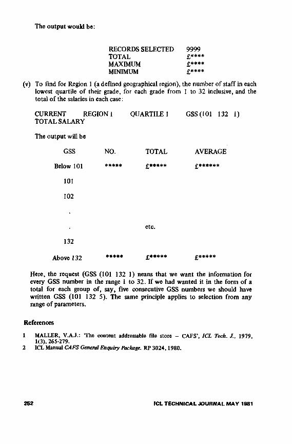
The output would be:

RECORDS SELECTED 9999TOTAL £##)01(MAXIMUM £****MINIMUM £***:(:

(v) To find for Region 1 (a defined geographical region), the number of staff in each lowest quartile of their grade, for each grade from 1 to 32 inclusive, and the total of the salaries in each case:

CURRENT REGION 1 QUARTILE 1 GSS(101 132 1)TOTAL SALARY

The output will be

GSS NO. TOTAL AVERAGE

Below 101 £*>11*** £******

101

102

etc.

132

Above 132 ***** £***** £*****

Here, the request (GSS (101 132 1) neans that we want the information for every GSS number in the range 1 to 32. If we had wanted it in the form of a total for each group of, say, five consecutive GSS numbers we should have written GSS (101 132 5). The same principle applies to selection from any range of parameters.

References

1 MALLER, V.A.J.: The content addressable file store - CAFS\ ICL Tech. /., 1979, 1(3), 265-279.

2 ICL Manual CAFS General Enquiry Package. RP 3024,1980.


Giving the computer avoice

M.J. UnderwoodICL Research and Advanced Development Centre, Stevenage, Herts

Abstract

Recent developments in semiconductor technology, together with advances in digital signal processing, have led to silicon chips that talk. Important though the techniques for speech generation are, their successful and widespread use in commercial computing systems will depend upon their careful incorporation into the overall systems design. This paper describes a systems approach to giving the computer a voice that will enable the end- user to obtain information easily and accurately. The first part of the paper is concerned with an analysis of requirements, with particular emphasis on the needs of the end-users. The concept of a speech subsystem as a modular component is described, together with some details of its prototype implementation. Some indication is given of the current and future applications for a computer with a voice. Spoken output from computers is likely to play a more important role in the future as the pattern of computer usage moves towards more human-oriented information processing.

1 Introduction

Speech has evolved as man’s most natural and important means of communication. Spoken communication developed much earlier than the written form, yet when it comes to the communication between man and his information-processing artefact, the newer written form is dominant. Why should this be? The answer probably lies in the different nature of the two means of communication. The evolution of speech is deeply interconnected with the evolution of human behaviour as we know it to-day. Organised human life without speech is inconceivable. Because it is so much a part of us it may be very difficult for us to be introspective about it and to understand it fully. As a means of communication it is informationally much richer than writing. Writing can be be regarded as a sub-set of natural human communication and this has led to it being mechanised much earlier. The ability to generate speech, as opposed to transmitting or recording it, has had to await the arrival of the information processing age.

There are two aspects to spoken communication, its generation and its understanding. Eventually the techniques for the automatic execution of both of these processes will have been developed to the point where people will be able to communicate naturally with computers; it is likely to be many years before this is achieved. Indeed, it could be argued that such a situation is unnecessary and undesirable, since the reason for designing information processing systems is to complement


man rather than copy him. Nevertheless, as more people come into contact with computers in their everyday lives there is a need to improve the means of man- machine communication. This paper is concerned with the requirements for giving the computer a voice and with the solution that has been developed in the ICL Research and Advanced Development Centre (RADC). The aim has been to design an intelligent speech controller that provides the necessary facilities for speech output in the commercial computing environment. The recently announced semiconductor ‘speaking chips’ have been designed for different purposes to meet mass- market requirements.

2 Speech as a communication medium

As a means of communication, speech has both advantages and limitations and it is important to understand these before attempting to design speech output equipment.

First, the advantages, as these will play an important part in determining how speech output is used. Speech is an excellent medium to use for attracting a person’s attention, even though their eyes are occupied with another task: it is very difficult to block the auditory channels. It is excellent also for broadcasting information simultaneously to many people as it does not require direct line of sight. It can also be a very private means of communication if played via a headset directly into the listener’s ear. Finally there are very extensive speech communication networks in existence — the national and international telephone networks — and it would be very attractive to be able to use these for computer-to-man communication without the need for equipment such as modems. Every telephone would then become a computer terminal.

An important limitation is imposed by the fact that the rate of speech output is controlled primarily by the speaker and not by the listener, which means that, unlike printed output, speech output cannot be scanned. Therefore computers, like people, should talk to the point. Another arises from an interesting property of the human processing system, the restricted capacity of the short-term memory, typically seven items.1 This places a limit on the amount of information that can be presented to a listener at any one time if he is to remember it well enough to do something useful with it, such as write it down. A further characteristic is that speech leaves no visible record and therefore is best suited to information which is rapidly changing or ephemeral.

The main conclusion to be drawn from this is that speech should not be regarded as a replacement for existing means of machine-to-man communication but as a complementary channel, best suited to the transmission of certain types of information.

3 Requirements

The requirements of three groups of people have to be considered: the user (i.e. the listener), the programmer and the equipment supplier. The primary objective of the user is to obtain information easily and accurately, whilst the programmer is


concerned with what the machine is going to say and how. The objective of the equipment manufacturer is to supply and support the requirements of the listener in a cost-effective manner. The requirements of these three groups affect not only the choice of speech output technique but also the way any speech subsystem is interfaced and controlled. In addition, the use of speech may have implications for the design of the system which uses it. For example, the information held on a file may need to be different to allow spoken output as opposed to printing.

3.1 Listener’s requirements

The way in which the information is presented is as important for the listener as is the method of speech production. Traditional methods of testing speech communication systems such as telephones or radio have relied extensively on articulation tests. In order to strip speech of the important contextual clues that enable a listener to infer what was said even though he did not hear it properly, articulation testing consists of using isolated words spoken in an arbitrary, linguistically nonsignificant order. This approach falls a long way short of assessing the usefulness of the communcation channel for genuine human conversation. So it is with computergenerated speech also. A system that can produce individually highly intelligible words, for example some random-access method of wave-form storage, will not necessarily produce easily understood speech when the individual words are assembled to make a sentence. Context plays an important role in speech perception: we are all familiar with the anticipation of football results from the way the newsreader reads them, giving different emphasis to teams with significant results, like a scoring draw.

In English, emphasis is signalled largely by changes in the prosodic features of speech, namely rhythm (rate of speaking) and intonation (voice pitch). Moreover, these changes are used to signal the meaning of a sentence. Thus a rising pitch at the end of a sentence often denotes a question. Consequently the prosodic aspects of spoken messages from computers should conform to normal human usage, otherwise there is the possibility that the listener may infer the wrong meaning.

It could be argued that it will be some time before we need true conversational output from computers, as they largely contain information of a highly structured and often numerical nature and consequently control over prosodic aspects is not important. However, a series of comparative experiments at Bell Laboratories2 showed that people’s ability to write down correctly a string of computer-generated telephone numbers was significantly improved if the correct rhythm and intonation were applied. Telephone numbers that were made from randomised recordings of isolated spoken digits were judged by the listeners to sound more natural but produced more transcription errors.

This raises the question of what the voice should sound like. There are several aspects to describing speech quality and these can be factored into two main headings: those that contribute to the understanding of the message and those that do not. In commercial systems the prime requirement is for good quality speech that is easy to listen to and does not cause fatigue on the part of the listener. This means that it must be clear and intelligible and possess the correct prosodic features that


facilitate understanding. The non-message related factors include such things as the fidelity of the voice — does it sound as though it was produced by a real vocal tract as opposed to an artificial one? — and the assumed personality of the character behind the voice. This arises from the fact that there is much more information conveyed by the voice than the text of the message being transmitted: for example, mood, character, dialect and so on. Whilst the message-related factors determine the understanding of the message, the non-message related factors are likely to determine human reaction. There is much to be said for providing a computer voice which is understandable but which possesses a distinctly non-human characteristic to remind the listener that it is not another person speaking. The balance of importance between the message-related and non-message related factors may well depend on the application, yet again indicating the need for a flexible voice output technique.

Another relevant aspect is the way that words are used to form messages. On a VDU screen the interpretation of a string of numerical characters is determined by the context or the position of the characters in a table of values. Thus 1933 could be a telephone number, a quantity or a year (or even a rather aged line-printer) and there might be no distinction between these representations on the screen. For this to be readily assimilated in a spoken form, however, the style of presentation should match the nature of the number, thus:

telephone number one nine three threequantity one thousand nine hundred and thirty threedate nineteen thirty three.

A speech sub-system which provides control over the prosodic aspects goes a long way towards providing a sufficient degree of flexibility to generate different numerical forms easily.

Other timing considerations have an effect on the listener and imply constraints in the way that any speech subsystem is controlled. Once started, speech output must be continuous with pauses only at semantically significant points like phrase and sentence boundaries. These pauses probably help the listener get the messages into and out of his short-term memory and, as every actor knows, the timing of these pauses has to be accurately controlled. The insertion of pauses at random is likely to have a disturbing effect on the listener and too long a pause may mislead him into thinking that the speech output has finished.

Another timing consideration is the speed of response to a listener’s reaction. Because of the transitory nature of speech, together with the limitations of the human short-term memory, the listener must have the ability to cause the system to repeat the last message. As the use of speech is likely to be in interactive communication, delays of several seconds which are common and are acceptable in VDU- based systems will be quite unacceptable; the response to requests like ‘repeat’ or ‘next please’ must be short, of the order of 0-5 seconds. The implication of all these considerations and constraints is that computer output of speech must be controlled by an autonomous subsystem and not by a general time-sharing operating system which has to satisfy many competing demands for processing power.


3.2 Programmer’s requirements

The listener’s requirement for spoken output that is easily understood and remembered implies a controllable means of speech output. The programmer’s task is to control this from the information and data available to him. The detailed control of flexible speech output is complex and requires a good knowledge of speech science and related topics. The programmer should be shielded from the details of how rhythm and intonation are controlled, but he should have available the means to control them. This principle can be extended to providing a means of specifying different types of numerical output and leaving the speech subsystem to work out how they should be done. The kind of interface envisaged therefore is similar to and an extension of the kind provided for the control of VDUs, where the programmer has the options of choosing lower case, italics, colour, flashing characters and so on. If the programmer is provided with an easy-to-use interface it is much more likely that he will be able to play his part in satisfying the listener’s requirements.

The ideal in speech production would be the ability of the system to say anything that could be printed, which would imply the ability to generate speech from text. Techniques for doing this are being developed3 but until they have matured to the level of commercial acceptability, any speech subsystem is going to be working with a restricted vocabulary of words and phrases. If the subsystem is to be responsive to changes in a user’s business which lead to changes in the vocabulary, for example the introduction of a new product with a new proprietary name, there must be provision for changing the vocabulary easily.

3.3 Manufacturer’s requirements

The equipment manufacturer has some requirements to satisfy in addition to the commercial ones of meeting his customers’ requirements in the most cost-effective manner. One of the most important is the connectability of the equipment. Ideally it needs to be connectable to existing systems with the minimum amount of disruption, preferably using an existing channel.

The requirement to be able to supply new vocabularies to meet changing customer requirements means that vocabulary up-dates should be supplied on conventional computer media so that they can be loaded like new software. Moreover, a support service has to be provided with suitably trained staff that can carry out this vocabulary preparation. An important requirement here is that if the vocabulary is derived from real human speech, then access to the original speaker must be maintained and facilities provided to match new utterances to ones that have been provided some time previously: it is well known that speakers’ voice characteristics change with the passage of time.

Although initial systems will use data derived from real speech, the long term requirement of synthesis from text, to handle name and address files for example, must be considered. Thus it is important for the manufacturer to choose a speech output technique that can be enhanced to meet this future requirement.

ICL TECHNICAL JOURNAL MAY 1981 2S7

4 RADC speech output project

4.1 Speech generation technique: general considerations

In summary, a good speech output system must have the following properties:

(i) it must be capable of producing intelligible speech(ii) the rhythm and intonation must be under programmer control

(iii) the storage requirements for the vocabulary must be reasonable(iv) the technique used for the speech generation must be capable of

enhancement to meet later expanded needs such as synthesis from text.

The simplest of all methods of speech generation is the use of prerecorded words and phrases which can be called in the appropriate order from storage. This has been used for small-vocabulary applications quite successfully but it does not meet the above requirements very well. The rhythm and intonation cannot be controlled without repeating the items in different forms; the storage demands are large, a minimum of 20000 bits being needed for one second of speech; and the technique cannot be expanded to meet the needs for large vocabularies like names and addresses.

A satisfactory technique should use some method of synthesising spoken words and phrases from more basic material and should be modelled on the human speech production process. The best method seems to be that of formant synthesis4 ; this is the one chosen for the RADC project and will now be described.

4.2 Formant synthesis

The formant description of speech models the acoustic behaviour of the vocal tract in terms that are related to what the speaker does with his vocal apparatus when speaking, rather than to capture the detailed wave form of the spoken sound. The primary energy in speech comes from the flow of air from the lungs. In voiced speech (e.g. vowel sounds) the flow of air through the vocal cords causes them to vibrate at a rate determined by the air flow and the muscular tension applied to the cords. The resulting puffs of air excite the resonances of the air in the vocal tract, the frequencies of which are determined by the positions of the articulators, i.e. tongue, lips, jaw. In unvoiced speech (e.g. s, sh) the flow of air through a narrow gap in the vocal tract produces a noise-like sound whose frequency content is determined by the position of the articulators. The formant description of speech is a way of describing the frequency spectra of speech sounds in terms of the positions and amplitudes of the dominant peaks in the spectrum (Fig. 1). As the articulators move from one position to another, the formant peaks move accordingly, but because the articulators move much more slowly than the vibrating air molecules, a formant description of speech is much more compact than that of the acoustic waveform. A formant synthesiser takes as its input a formant description of speech (Figs. 2 and 3) and computes the values of a waveform according to the mathematics of the model incorporated within it.


frequency, kHz

frequency, kHz

frequency, kHz

Fig 1 The formant description of speech describes the transfer function of the vocal tract in terms of the positions of the peaks in its frequency spectrum. The positions of these peaks depend upon the positions of the articulators (tongue, lips, etc.). The spectrum of a speech sound is the product of the spectrum of the source and the transfer function.

a Frequency spectrum of vocal cords during voiced speech b Transfer function of the vocal tract for a typical voiced sound c Frequency spectrum of the resultant speech sound

Formant synthesisers have been studied and used extensively by speech scientists.5Typically four formants (the four lowest resonant frequencies) have been found tobe sufficient to produce highly intelligible speech. Three formants are sufficient for


telephone use with its restricted bandwidth. The formant description of speech is only an approximation to what happens in real speech, but if sufficient care is taken in deriving the formant parameters from real speech it is almost impossible to distinguish resynthesised speech from the real speech from which it was derived.6 This more than meets the need to produce highly intelligible speech. Moreover the formant description of speech is a very compact one and good quality synthesised speech can be produced from a data rate as low as 1000 bits/second.

Time(ms)

ST F0 F1 F2 F3 A1 A2 A3 F AF

10 0 140 0 0 6 -48 -4 8 0 -4820 138 234 2530 125 2840 119 156 1638 2691 31 -30 -3050 103 195 1599 265260 102 234 1560 2730 34 -42 -2470 2769 37 -2480 101 1521 -3090 1482

100110 100 546 1638 2808 40 -12 -12120 101 585 - 6130 102 624 1560 43 -12140 103 1521 - 6 -18150 104160 663 1404170 702 1326 2847180190 1287 2886 -24200210220 105230240 104250 103 1326 -12260 100 663 1404 2647270 1521 40 - 6 -18280 99290 100 1560 2808300 624 1638 2769310 1716 -12320 101 546 1872 2691 37 - 6 -12330 1950 -12 -18340 507 2028350 2067 -18360 468 2184 2652 34370 429 2223 -24380 100 390 2262 -24

Fig. 2 continued on facing page


Time ST (ms)

F0 F1 F2 F3 A1 A2 A3

390 101 2691400 102 2301 -18 -30410 103 351 2106 -24420 104430 105 312 1443 2652 -30440450 1521 2769 -36 -24460 106 1482 31 -24 -18470480 1443 -24490500 120 0 0 0 6 -48 -48

Fig. 2 Synthesiser parameters for the word 'NINE'Each line represents 10 ms of speech. Blanks indicate that the parameter value remains unchangedST: Sound type 0 = voiced, 2 = voiced fricative, 3 = unvoicedF0: pitch of the voice in HzFI, F2, F3: first three formant frequencies in HzA1: overall amplitude in dBA2, A3: relative amplitudes of F2, F3 in dBF: unvoiced sound typeAF: relative amplitude of unvoiced sound.

The use of formant synthesis also meets the requirement of being able to control prosodic aspects. The parameters that are used to control a formant synthesiser (Fig. 2) can be manipulated independently of one another, and these include the voice pitch. Thus in order to modify the pitch of the synthesised voice it is necessary to change only the values corresponding to this parameter. The speed of talking can be varied by altering the rate at which parameters are fed to the synthesiser. A typical up-date rate of parameters is 100 times a second. If the same parameters are sent at twice that rate, the synthesiser model is driven more quickly and the resulting speech is twice as fast but with none of the ‘Donald Duck’ kind of distortion associated with speeding up a tape recorder. In practice, the control of speaking rate is more complex than the simple overall alteration of the rate at which parameters are supplied to the synthesiser. The perception of some speech sounds is influenced strongly by dynamic effects, that is by how rapidly the articulators move from one position to another, whilst the perception of steady-state sounds like vowels is largely independent of changes in the rate of speaking. The need to control carefully the way speed changes are carried out is a very good reason for shielding the programmer from this kind of complexity.

It is not only the synthesiser design that determines the quality of the speech produced, but also the values of the parameters that drive it. There are three main sources of data from which these values can be derived. The first is by analysis of real speech. This has been studied extensively and has been found to be difficult to


automate completely.7 With careful manual intervention and editing, excellent quality speech can be produced but it is an expensive process. The RADC approach, to be described later, is to employ a combination of computer and manual methods and has proved more cost-effective.

52-

O OO Ooo_ _ o o o o o o o o o u w O O O O . -

. 0 0 0 0 0 00

Dn□□ 0 Do□ □□ O 0 r

x x x x x x X x X x x x x x x x x x x x x x x

0 0 0 0 0 0 0 00 0 0 0 0 0

□ □ o

0 0 0 0 3rd formant

00_o o □□

* X X s

Do d o ° q □ 2nd formant

xx xx x x xx x1st formant_j______1______1______1______L-

0 50 100 150 200 250 300 350 400 450 500time, ms

Fig. 3 Formant representation for the word 'NINE'

Another method is what is called synthesis-by-rule.8 This is based on the linguistic premise that a spoken utterance can be described in terms of discrete sounds, in the same way that a written message can be constructed from the letters of the alphabet. Every speech sound can be described in terms of a set of synthesiser parameters, together with rules that determine how the parameters are modified by the context of the preceding and succeeding sounds: the dynamics of the articulators are such that these cannot be moved instantaneously from one position to another. The input to a synthesis-by-rule system is a string of phonetic elements specifying what has to be said, together with some parameters that specify rhythm and intonation. Thus synthesis-by-rule is a completely generative method, but the present state of the art is such that it requires trained and experienced operators to produce good quality speech.

The third method is synthesis from text. Synthesis-by-rule enables the programmer to specify any speech output but requires control at the phonetic level. Synthesis from text takes the method a stage further by providing a mechanism for converting the orthographic representation into a phonetic one. The difficulty here is that English in particular is a mix of rules and exceptions — a classic example is ‘- ough’, for which there are several pronunciations depending on the context. Synthesis from text will provide the ultimate means of speech output, enabling material to be printed or spoken from essentially the same data. But because of the vagaries of pronunciation it is unlikely that any automatic system will be capable of producing the correct one for all names and addresses, for example. It is likely that an intelligent speech subsystem would deal automatically with the common names but that


some additional pronunciation guide would be included with other items. This would be phonetic in character and would occupy no more than an amount of file space equivalent to that of the orthographic representation. At present, synthesis from text has not matured sufficiently to be commercially acceptable or economically viable, significant amounts of computation being needed to convert from text to speech, along with the rules necessary to impart the correct emphasis.

The requirement for commercial systems is not to be able to read English prose but to speak aloud information of a much more restricted kind and content, such as ‘the customer’s name is . . . and the address is . . . ’.

Until the completely generative approaches of speech synthesis have developed to the point of commercial quality and viability, speech output based upon formant synthesis will use parameters derived from real speech, giving good quality speech at modest storage costs with the desired degree of control and flexibility. When the time comes to use the generative approaches it will still be possible to use formant synthesis, but controlled in a different manner. Thus the use of formant synthesis provides an open-ended development path for customer and supplier alike.

4.3 Hardware implementation

Analogue techniques were used in the early synthesisers.8 Bandpass filters whose centre frequency could be controlled were used to simulate the formant resonances and these were excited by either a controllable periodic source or a nosie source, corresponding to voiced and unvoiced speech, respectively. Analogue circuitry made from discrete elements is prone to drift and needs careful setting up and subsequent adjustment. The RADC decision, taken in the early 1970s, was to build a synthesiser using wholly digital techniques. At that time an economical design could be produced only by using a multiplexed technique whereby the synthesiser could be shared among a number of channels, because of the stringent need to compute a new wave-form sample every 100 jus. A design was produced that enabled 32 independent output channels to be supported simultaneously.9 Subsequent developments in semiconductor technology have made it possible to build a synthesiser using a standard microprocessor and this has formed the basis of the current implementation. It is now possible to put a formant or other synthesiser on a single chip and several semiconductor manufacturers have developed such chip sets for mass-market applications including electronic toys. However it is the control aspects that are important for the commercial market and consideration of these was a leading factor in the design of the RADC system.

Fig. 4 shows the prototype synthesiser controller which has been developed to provide the degree of flexibility and control required in a high-quality system. The aim has been to design modular low-cost equipment that could be readily attached to existing computer systems and easily enhanced to provide a multichannel capability. The three main components are an 8-bit microprocessor with store and I/O ports, a synthesiser and Touch-Tone signalling detector and a line unit to interface to telephone lines.

The controller uses an 8-bit industry-standard microprocessor with 64 kbytes of RAM storage and serial and parallel interface ports. The serial port is used


for the mainframe link and the parallel ports for controlling the synthesisers, signalling detectors and line units. Although two independent speaking channels are shown, only one has been implemented in the prototype. The storage is used for both code and vocabulary data, there being room in the prototype for approximately 100 seconds of speech, or 200 words of half-a-second duration. As this is considered to be adequate for many applications, no particular effort has been made to produce a more compact representation of the data although there is scope for reducing the data rate further.

P0 lines PO lines

Fig. 4 Block diagram showing the main hardware units of the prototype speech output subsystem


The synthesiser uses another microprocessor with associated support circuitry in an implementation of the technique used by Underwood and Martin.9 In many applications it will be necessary for the end-user to have some means of communication with the speech subsystem. In the long term, speech recognition techniques10 will have matured sufficiently to make two-way speech communication possible. Until then the input will be by means of a limited function keyboard, similar in concept and lay-out to that used with Prestel. However, the signalling method normally used in voice response systems (MF4) employs the selective use of two tones out of eight, as used in Touch-Tone telephone dialling in America. Until that signalling method or some other becomes an integral part of every telephone, the keypad will be a separate portable unit that acoustically couples to the microphone of a standard telephone handset. The synthesiser board incorporates circuitry to decode the pairs of tones that are transmitted down the line by such a terminal.

The line units provide the necessary interfacing protection between the speech subsystem and the telephone network. The unit has provision for both receiving and making telephone calls under program control.

4.4 Synthesiser control

The code in the controller performs three types of function:

(i) detailed control of all the I/O: maintaining data flow to the synthesiser, receiving data from the Touch-Tone detector, controlling the line unit and servicing the communications protocol

(ii) provides the high-level interface for control of speech output(iii) provides the interaction management, independent of the mainframe.

The most interesting of these is concerned with the control of the speech output. Given that the synthesiser approach enables the style of output to be controlled, the question arises as to how this should be done. It is envisaged that different levels of control are appropriate to different application, so a number of levels have been implemented.

At the lowest level, each vocabulary item can be called by item number; these items can be of any length and any one can be a phrase, a word or a part word. This is a most flexible arrangement and enables the best compromise to be made between naturalness and efficient use of the store. If all the words in a particular phrase appear nowhere else in the vocabulary, the most natural utterance results from storing it as a complete phrase. If a word or part word occurs in several contexts, more efficient use can be made of memory by storing the item once only and concatenating it with different vocabulary elements to form complete words.

It is likely that when a vocabulary item is used in different contexts it needs to be emphasised differently. For example, the ‘six’ in the word ‘six’ is shorter than the ‘six’ in ‘sixteen’. To accommodate changes in emphasis two optional control characters can be used to control the pitch and speed of each item independently. As noted earlier, changes in the rate of speaking cannot be applied uniformly to the


speech, so the vocabulary data contain information that allows speed changes to be carried out in an appropriate manner.

Whilst this level of control provides the programmer with a powerful way of changing the speech and at the same time shelters him from the details of how it is done, there is a need for some commonly-used strings of vocabulary items to be handled more easily. One example is the different forms of numerical output which are likely to form a part of most application vocabularies. To save the programmer from having to remember and to use explicitly the rules for generating quantities — the machine should say ‘thirty three’, not ‘threety three’ — these rules are coded in the controller and enable the different types of output to be generated automatically. Thus:

N(digit string) causes the digits to be output with suitablepauses and prosodic changes to make them easily understood

0(digit string) gives the ordinal form: first, second . . twenty-fifth . .

Q(digit string) causes the digit to be spoken as a quantity e.g.one hundred and seventy two

Another feature is the message facility, whereby a string of user-defined vocabulary items can be referred to by a message number. Moreover, this facility is parametrised so that variable information can be included.

A particularly important requirement for a speaking system is that the listener must be able to cause the last message to be repeated. It is a natural human reaction, when asked to repeat something, for the speaker to say it again more slowly and deliberately, so that the listener will have a better chance of understanding it the second time. The controller is provided with a facility which mimics this aspect of human behaviour.

The controller also provides a means for requesting and handling Touch-Tone data and for controlling the line unit. In order that the controller can react quickly to events such as the input of data or detection of ringing current on the line it must do so autonomously without reference to the mainframe. The prototype enables sequences of instructions, using all the facilities which it controls, to be stored and actioned. This enables the listener and the controller to interact independently of the mainframe until a point is reached at which mainframe action is required, like the retrieval of some stored information. This is analogous to the filling in of a form on a VDU screen, which goes on under local control until the ‘send’ key is depressed.

4.5 Vocabulary preparation

Until the truly generative approaches to speech synthesis are mature enough to produce the high quality speech required for commercial systems, thereby enabling the computer user to develop his own vocabularies, vocabulary preparation will be a specialised bureau-type service that will have to be provided by the supplier of the


speech subsystem. Vocabulary preparation is the crucial factor in using a formant synthesiser, as it largely determines the quality of the synthesised speech. The major requirements here are:

(i) it must be capable of producing good quality speech;(ii) the service must not be costly to operate, either in terms of the equip

ment it uses or the time it takes;(iii) the level of skill required to operate it must not be great;(iv) it should contain facilities to enable vocabulary up-dates to be closely

matched to earlier vocabulary items as a customer’s requirements change.

The analysis of real speech to provide parameters for a formant synthesiser is a complex process and is only one stage in preparing a vocabulary for a particular application. The major stages are as follows.

The first stage is to list and analyse the utterances that have to be made and to prepare a script for recording purposes. Although the formant synthesis approach enables synthetic speech to be massaged to suit the context, experience in vocabulary preparation shows that the best results are produced if the words are recorded in a context which is identical or as similar as possible to the context in which they are to be used. The next stage is to produce a studio-quality recording of the script, using a speaker with good voice control. Information that is lost at this stage cannot be recovered, so it is worth taking care with this part of the process.

Once the recording has been checked for correct pronunciation, signal level etc., it is transferred to a conventional disc file via an analogue-to-digital converter. The resulting digital recording is listened to and then split up for subsequent processing. A suite of analysis programs has been developed at RADC to produce files of synth- siser parameters, which then require manual editing. The editing process uses an interactive program that enables the parameters to be modified and the resulting synthetic speech to be listened to. The need for this editing arises because the analysis programs do not handle all speech sounds equally well, so that mistakes have to be corrected and omissions repaired. More importantly, such processes as defining the boundaries of vocabulary items and adjusting the balance (loudness, pitch etc.) between them require human skill and judgement. The balance of mantime and machine-time in vocabulary preparation is such, however, that further automation of the process in its current form would not be cost-effective.

The final stage of the vocabulary preparation is the encoding of the synthesiser data into its compact form and the preparation of files suitable for loading into the synthesiser controller.

4.6 Current status

The project has reached the stage where the design principles of all the required software and hardware components have been verified with the prototype implementation. A number of trial applications have been modelled using simulated data


bases. The next stage is to mount realistic field trials in order to gain first-hand experience in applying the techniques to practical computing tasks.

S Applications

The kinds of situation in which speech output could be valuable have been indicated earlier in the paper and are summarised in Table 1. Several systems have been produced commercially, particularly in the USA, within the following fields of application:

order entry by mobile salesmenstatus reporting, for example for work in progressbanking enquiries and transactionscredit authorisationspares locationticket enquiry and reservation direct mail order.

Most of these systems have been remote data entry or database enquiry, where voice has been the sole means of communication with the user. So far, speech output has not been integrated into existing terminal facilities. Once this happens there are likely to be many instances where the use of voice provides a valuable adjunct to those facilities. Some initial applications might be to the following tasks:

(i) to provide verbal feedback of data that has just been entered, allowing complementary use of eyes and ears for checking;

(ii) to provide instructions to operators in large computer installations;(iii) where a screen is already full of information and a simple message is required

to guide the user, for example, Computer Aided Design (CAD) or Computer Aided Instrumentation (CAI)

Table I. Situations where speech output could be valuable

The end-user is mobile, so that any telephone could become a terminal using a highly- portable acoustically-coupled keypad.There is a requirement for a large number of widely distributed users, particularly if the access by any one user is relatively infrequent and does not justify the use of an expensive terminal.The volume of data to be input or output as part of any transaction is small and relatively simple in nature.The information to be disseminated is constantly changing (hard copy would be out of date).There is a need for a database to reflect an up-to-the-minute situation. This includes order entry systems for products with a short shelf-life, as well as stock control systems. A service has to be provided on a round-the-clock basis.In announcements or alarms where the attention of one or more individuals must be drawn to a message.Where a message needs to be communicated privately to a user.


It is inconceivable that such an important and powerful means of communication as speech should not play a significant role in the man-computer communication of the future. Ultimately speech output and input are likely to be an integral part of every computer, just as VDUs are today. However, from our current viewpoint where we are only just becoming accustomed to the speech technology that is now available it is very difficult to predict just how widespread its use is going to be.

Two main factors are likely to affect the use of speech in the long term. The first is what computers will have to talk about. Developments such as CAFS11 mean that it is now possible to design information systems that are able to answer requests quickly enough to make conversational working a real possibility. Speech output needs the change in emphasis from data processing (computer-oriented facts) towards information processing (human-oriented facts) that is now taking place.

The second factor is the human reaction to the idea of computers that talk. Consider the likely effect on a computer operator for example when the computer booms out in an authoritative voice ‘load tape three six seven five’. Such a message may well be acceptable when displayed on a screen, but the wrong tone of voice from the computer may have an effect which is entirely contrary to the user-friendly one we are trying to create. Although we cannot predict what the human reactions to computer speech will be, we are now in a position to use the technology in real- life situations in order to assess them. The next step forward is to start to apply speech output to practical use.

6. Conclusion

This paper has attempted to show that there are a number of aspects other than the purely technological ones that have to be considered when designing equipment to give a computer a voice. Good design is a compromise between ends and means, goals and constraints.12 When designing machines that will use speech, with all its linguistic, cultural and psychological implications, it is clear that consideration of human requirements must play an important role. Requirements can often be met without regard for cost; but the solution described in this paper not only satisfies these human requirements but does so in a highly flexible, modular and cost- effective manner that provides a development path for the future.

Acknowledgments

The work described in this paper is the result of a team effort in RADC over a number of years and the author acknowledges with gratitude the contributions of all those who have participated. Particular mention should be made of M.J. Martin who has been responsible for the design and implementation of the equipment, and of the late Roy Mitchell for his insight and guidance; and of Gordon Scarrott, Manager of RADC, for creating and sustaining the environment in which the work was done. Grateful acknowledgments are due also to the Department of Industry which, through the ACTP scheme, gave valuable support in the early stages of the project.


References

1 MILLER, G.A.: The magical number 7, plus or minus two. Psychological Rev., 1956,63, 81-97.

2 RABINER, L.R., SCHAFER, R.W. and FLANAGAN, J.L.: Computer synthesis of speech by concatenation of formant-coded words, Bell System Tech. J. 1971,50,1541- 1588.

3 ALLEN, J.: Synthesis of speech from unrestricted text, Proc. IEEE 1976,64 (4), 433- 442.

4 FLANAGAN; J.L., COKER, C.H., RABINER, L.R., SCHAFER, R.W. and UMEDA, N. Synthetic voices for computers, IEEE Spectrum 1970, 22-45.

5 FLANAGAN, J.L. and RABINER, L.R. (Eds), Speech synthesis, Dowden, Hutchinson and Ross, 1973.

6 HOLMES, J.N.: The influence of glottal waveform on the naturalness of speech from a parallel formant synthesiser, IEEE Trans. Audio & Electroacoust. 1973, 21, 298-305.

7 SCHROEDER, M.R.: Parameter estimation in speech: a lesson in unorthodoxy, Proc. IEEE 1970,58 (5), 707-712.

8 HOLMES, J.N., MATTINGLEY, I.G. and SHEARNE, J.N.: Speech synthesis by rule, Language & Speech 1964,7(3),127-143.

9 UNDERWOOD, M.J. and MARTIN, M.J.: A multi-channel formant synthesiser for computer voice response, Proc. Inst. Acoust. 1976, 2 - 1 9 - 1 .

10 UNDERWOOD, M.J.: Machines that understand speech, Radio & Electron. Eng. 1977, 47 (8/9), 368-378.

11 MALLER, V.A.J.: The content-addressable file store CAFS, ICL Tech. J. 1979, 1(3), 265-279.

12 SCARROT, G.G.: From computing slave to knowledgable servant, Proc. R. Soc. London Ser. A . 1979, 369,1-30.


Data integrity and the implications for back-up

K.H. MacdonaldICL Product Planning Division, Putney, London

Abstract

The paper considers the ways in which errors can occur in the recording of information on magnetic tapes and discs, the methods available for detecting such errors and the possibilities for protecting the user of the information against possible ill effects. From a consideration of the high standard of reliability of modern equipment the conclusion is reached that the best policy for back-up of data held on a magnetic disc is to hold a second copy on a second disc.

1 Introduction

The term ‘data integrity’ means many things to many people. To engineers it is an expression of the incidence of transient or permanent errors on magnetic media. To a user it implies quite simply that his data has not been lost or abused by others and that it retains its accuracy. Generally it is assumed that data will maintain these characteristics irrespective of who else may have raked over the data since the user last consulted it.

The term is also applied to many other aspects of computing and of information distribution, for example to indicate that data despatched has not been corrupted during transmission. The essence of the problem of maintaining data integrity is the corruption of stored data and the causes and cures for this.

The vagueness of the definition leads to parallel vagueness about the fundamental problem and in turn to confusion about the ownership of this problem. The complete spectrum of those involved in computing are blamed for perceived failures in data integrity. As with the equally obscure problems of security and privacy, responsibilities are dispersed throughout the data processing community. There are contributions to the problem at every stage in the development of a computer system and application.

2 Why is there a problem?

Computers started as computing machines. Without delving too deeply into the history or philosophy of computing, it is clear that modem computers are mostly used for storing, maintaining, manipulating and providing access to data or informa-


tion. Examination of the work done by a typical ‘mill’ clearly shows that most of the time is not spent on computation. Rather the manipulation of information dominates, including in this the multitude of operations needed to provide access to information to an authorised enquirer, changing information and protecting the information from abuse. Computers are ‘inventory systems’ in which data is the commodity kept in the inventory. They are thus essentially record keeping machines.

It is commonly thought that, besides the investment in the computing equipment itself, a customer’s or user’s main investment is in the programs that he has developed. This often undervalues the investment that has been made in the creation of the data, and the human endeavour and computing time that have been spent on getting the data into the system, getting it right and keeping it right. There are many situations where what is contained within the store of a computing system is essentially an expression of the affairs of the enterprise. The commercial operation of the enterprise may not only be aided by the computer, but may be dependent upon it and upon the data contained within it.

What is increasingly evident from new product announcements and from the literature of the industry is that a shift has occurred away from the conceptual attachment of files to processors, towards the attachment of processors to files. Specialised processors now exist solely for the purpose of managing information storage, ranging from conceptually simple though intrinsically complex controller devices to functional subsystems such as, for example, the Content Addressable File Store.

To develop the inventory analogy further, the fundamental disciplines of managing an inventory apply equally to data. Stopping unauthorised persons from putting bad material into inventory or stealing material from inventory corresponds to the security and privacy functions. Knowing where the commodity is in the inventory is one of the main tasks of the data management system. Physical changes can occur, such as print-through on magnetic tape, random landing of heads on a spinning disc, deterioration of the storage medium, and prevention of this intrinsic decay is one of the most common interpretations of the term, data integrity. Taking account of corruption when it occurs, as it inevitably will, is data recovery. Just as it is necessary to take stock of a physical inventory from time to time, so it is necessary to review the contents of files, to reorganise them, preserving and simplifying their structure while eliminating those obsolete items that can be written off. This data management operation can serve to identify ‘rogue’ records and to allow their elimination or correction, and by this ‘refreshment’ of the files reduces the probability of intrinsic failure.

3 Data corruption and intrinsic integrity

There are three main contributors to the corruption of data within a storage system, namely:

(i) users’ programs and operating errors(ii) failures in the system such as hardware, supervisory software or data

management software(iii) intrinsic failures in the storage devices themselves.


Recovery is needed for all these circumstances and is a common problem. The solution to any one is equally applicable to the others. However, some consideration of the incidence of corruption suggests that the solution can be biased to provide a better service to the end user.

Data storage products are dominated by magnetic tapes and discs. Optical storage systems are beginning to appear but widely available and economical optical devices will not be with us for some time yet. If we concentrate on magnetic tapes and discs it is evident that the growth of computing is bringing conflicting demands for increased capacity, increased transfer rates, shorter access times to support higher performance or shorter response times, lowers costs, increased reliability and all the other virtuous attributes.

4 Magnetic tapes

Magnetic tape is the oldest really large-scale storage medium. All the usual curves can be drawn showing developments in the favourable direction over time of all the attributes. At a simple level, the basic cost is determined primarily by the maximum speed of stable motion of the tape itself; the difficulties of other problems such as that of starting and stopping the tape, and therefore the cost of overcoming these difficulties, increase as the tape speed increases. The total cost is made up of that of providing the tape speed, the acceleration and deceleration, the vacuum control, the resolution of the recording and the power needed to drive the whole system and increases almost linearly as the tape speed increases. Whilst the achievement of higher tape speeds has contributed to increased throughput, parallel increases in the density of information recording on the tape have enabled higher rates of information transfer to be achieved with lower tape speed than would otherwise have been the case. The cost of data transfer rate has in fact declined because the increase in packing density has allowed lower cost mechanisms to be used.

A basic problem that remains is the medium itself. This is long, flexible and flawed and the control of its movement at the required transport speed is the basic contributor to cost. The flexibility contributes to the complexity of maintaining a steady rate of movement; it also means that physical shocks, applied for example by the capstan, can easily migrate to other parts of the system such as over the heads. All the vices and virtues combine to give a sub-system which we tend to take for granted and frequently scorn but which is actually very complex and probably very long lived. The history of magnetic tape is littered with confident predictions of their early total replacement, all premature.

Early tape units recorded information at very low density. I can remember the impressive demonstrations of magnetic recording that we gave by laying a strip of recorded tape under a thin piece of paper and sprinkling iron filings (‘Visimag’) over it. The individual bits could be clearly seen.

Such a demonstration would be difficult today because of the high packing densities, and the very small magnetic fields that are recorded. These early units depended for the reliability of their information recording on the massive signals that


could be generated at relatively low transport speeds. Each recorded bit was relatively large in comparison with the contamination or the flaws in the medium.

As information density had to be increased as a means of improving transfer rates and device utilisation, so in parallel it was necessary to ensure accuracy of information being recorded at the time that it was recorded. Reading-after-writing and parity are now taken for granted. Reading by a second head after recording allows comparison of the recorded data with what was to be recorded. If the data coding includes parity, then the need for such a comparison is avoided and the validity of the recording can be tested by a parity check. Parity, by including redundant information, allows the detection of either a ‘drop-out’ or a spurious bit. By increasing the amount of redundant information, possibly both laterally across the tape and longitudinally along its length, the sensitivity of the detection system can be increased to allow for double and even triple errors. Likewise the redundant information can be used to calculate what incorrect signals have been read, usually to a lower degree of resolution than the error detection system. These techniques are well documented.1

The essential integrity elements of the storage system were:

(i) Ensuring that information was correctly recorded before continuing.(ii) If information could not be correctly recorded in a particular place on the

tape, then that area of tape could be erased and the information recorded a little further down the tape.

(iii) On reading, the accuracy of the reading could be checked and if an error was detected, the tape could be backspaced and further attempts made.

(iv) If after several attempts the data still could not be recovered, the system at least knew that the data was faulty and had not attempted to process faulty information.

(v) Systems techniques such as the grandfather-father-son approach for file maintenance provided a simple, although time consuming, method of retrieving the situation.

(vi) Combinations of prelude and postlude information surrounding data blocks, in some cases with software recorded block numbers also, provided protection against the loss of a block.

As recording densities increased, so the likelihood of a transient error on reading the data also increased. The information recorded on the tape could well be correct, but the time taken to backspace and re-read could seriously reduce the productivity of the system. Thus, when phase encoded tape at 1600 bytes per inch was introduced, a coding system was provided which allowed the controller, if it detected a single bit error, to correct that error without the need to re-read. In providing this capability, the tape unit also acquired the ability to detect drop-outs of more than one bit in a data frame. The concept has been further enhanced in the Group Code Recording scheme, in which data appears to have been recorded at 6250 bits per inch. This is in fact an average apparent recording rate since the density of flux changes is about 50% greater. A coding scheme is used which allows error correction on the fly for any single or double combination of tracks simultaneously. Errors may be corrected in all 9 tracks of a single block, provided that they occur in combinations limited to 2 tracks at a time.


This tape system includes the automatic recording of synchronisation bursts of data at the beginning of each reel. This allows automatic adjustment of the reading circuitry when that tape is subsequently read, to allow for any small maladjustments of the recording mechanism. Within long blocks, bursts of synchronisation data are inserted to reset the error correction logic and thereby maintain maximum error correction capability. Because of the scope of the error correction facilities on reading, it is possible even to tolerate some errors during the writing of tape, thus minimising the backspace - re-write occurrences. At least one major manufacturer does this.

S Magnetic discs

Disc developments have been even more dramatic. Here the density of information recording has been increased not only in respect of the number of concentric tracks recorded on the disc surface, but also the density of the information recorded within a track. The majority of current disc drives today contain 300 to 600 information tracks per inch (compared with 9 tracks across half an inch of magnetic tape). Information within a track is recorded at densities that are typically 6000 bits per inch. Some recently announced disc units probably record close to 1000 tracks per inch, with information at densities close to 12,000 bits per inch around each track. Developments in new disc coating techniques as well as new head technology suggests that 2000 tracks per inch and 20,000 bits per inch are achievable in the medium term.

These data densities bring inevitable problems in their train. Increasing track density requires very close alignment of the head to the track and the need for very accurate positioning. The reasonable tolerances of mechanical positioners have been exceeded, with fine adjustment of the head position now being controlled by servo techniques. The high recording density leads to the requirement for the recording head to fly very close to the surface. Several specialist disc manufacturers illustrate this low flying height by suggesting that the engineering task is similar to flying a 747 around the world only an inch above the ground. The rate of revolution of the disc must be sufficient that readable signals are obtained. At high recording density this results in very high transfer speeds for the information flowing from the disc, or required to flow to the disc. Instantaneous transfer rates in excess of a million bytes per second are common, with some very large capacity units transferring at 3 million bytes per second and higher rates envisaged. These high rates of information transfer can cause indigestion in even large computer systems.

At the same time, the problems of manufacturing the disc media themselves have needed to be addressed. It has not been, for some time, practical to provide discs that are totally free of flaws. Manufacturers have overcome this problem by testing the assembled stack of discs, identifying flaws and, provided that the number of these is reasonable, assigning spare tracks to maintain the overall capacity of the unit. As densities have increased, so the problem of flaws has also increased to the point where it is prudent to assume that every track has a flaw. Assigning spare tracks thus becomes no longer adequate. Instead, spare sectors may be needed with


each track, with spare tracks used to cover those situations where flaw occurrences are such that the spare capacity of a track cannot handle the situation because several sectors must be re-assigned.

Error detection and correction coding systems have needed to be developed in parallel. Practical engineering considerations limit the feasibility of using a pair of writing and reading heads to give a “read-after-write” check. Instead a complete additional revolution of the disc may be needed, with the information read on the second revolution to check that the recording has been correct. ‘Defect skipping’ and ‘defect swallowing’ techniques hide the flaws from the user.

As the density of both tracks and data has increased, but particularly that of the tracks, it has been necessary to preserve a fixed relationship between heads, media and recorded information. A similar situation has been recognised for many years in the case of magnetic tape: even setting aside the intrinsic quality of the tape, it has long been known that particular formulations and head profiles are satisfactory in combination while others generate problems such as tape wear, head wear, “stiction” and so on. Reading and writing on the same transport usually gives best results. In the case of discs, the disc pack and the heads used to record and read the data on the pack need to be kept together.

Mechanical considerations limit the track density and information recording density that can be achieved on exchangeable units. The capacity of an individual drive in which the pack is exchangeable is limited in comparison with what can be achieved if the heads are permanently associated as in a “fixed” disc. Even at relatively modest track and bit densities the cost of units with the same capacity will be greater in the case of an exchangeable unit because of the mechanical linkages which must be provided, as well as the provision of a ‘cleaning’ system to minimise the build up of environmental contamination within the pack. An intermediate solution, in which the heads were contained within a closed exchangeable pack was introduced by one major manufacturer some years ago. This approach has not survived. Today, virtually all high density and high capacity disc storage devices use fixed media, in which the heads and discs are contained within a sealed environment. Exchangeable discs are thus limited to medium capacity devices or cartridges.

6 Reliability

To avoid withdrawing the heads and thereby reducing the access ‘stroke’, the heads must be able to land on the disc without causing a ‘head crash’. Having solved this problem and having adopted a fixed disc, with the heads permanently associated with the recording surfaces, additional mechanical simplifications can be applied which reduce cost and increase reliability. The systems advantages of exchangeable disc units are lost, although it is noted that many large organisations with large ‘disc farms’ have, for some time, been using exchangeable discs essentially as if they were fixed. Reliability improvements are noticeable when this is done.

The usual measures of intrinsic reliability are the Mean Time Between Failures, and the commonly quoted Data Integrity Parameters of the number of errors encountered during the reading of a large volume of data.


MTBF is a misleading statistic considered in isolation. It is affected by environment, usage and the other factors. In general, medium capacity exchangeable disc units demonstrate MTBF in the range of 3000 to 4000 hours. A typical medium capacity fixed disc unit, with double the capacity of the same sized exchangeable units, demonstrates MTBF of 8000 hours or more. The actual head and disc assembly itself, excluding the electronics and other support functions in the transport/drive, may have an MTBF between 15,000 and 20,000 hours. The reliability of the disc drive itself now exceeds the reliability of the electronic components of a small system. The most unreliable component in a medium sized fixed disc could well be the local disc drive control electronics.

Data integrity is normally specified for transient and irrecoverable (or hard) read errors. Transient errors are normally considered as those that are not repeated if an attempt is made to read the data again. The definitions are sometimes confused by the quotation of transient error rates that take account of data recovery through the use of a sophisticated error correction coding scheme. Typical data integrity parameters for discs are in the range of 1 error in 1011 or 1012 bits or bytes read, with transient errors normally an order of magnitude worse than hard errors.

The engineering approach to disc drive design usually first ensures that good data recording can be achieved and confirmed through a system of error detection. From the user’s standpoint, the priority is probably the detection of the error. The other priority is to provide a mechanism for correcting as many of the errors during reading as possible, in order to minimise the necessity for a further revolution and repeated reading and reduce the probability of unreadable data.

The big bogey for both discs and tapes remains the undetected error. I have been involved in many arguments where the inclusion in a specification of an Undetected Error Rate has been demanded. A theoretical analysis of the error detecting code and the recovery algorithms may suggest the irrelevant and trivial probability of a situation in which an error may not be detected or may be corrected incorrectly. This does not take account of the physical considerations. In any event, there seems little point in providing a specification parameter that cannot be measured. A fundamental characteristic of a undetected error is that it has not been detected and therefore cannot be counted. The circumstances are so remote that enhancing current detection codes is not very significant. In the context of actual data corruption the problem does not deserve consideration.

7 Occurrence o f corruption

The combination of MTBF and data integrity parameters implies very high standards of intrinsic reliability for fixed discs. The logical conclusion is that' failures of the device itself are unlikely to be a large proportion of the total population of incidents concerning data-recovery failures. Computer manufacturers are still addressing the intrinsic reliability issues and improvement in these can be expected. What is now clear is that in terms of ensuring access to data, the preservation of information paths and subsystem control functions is probably far more significant than the intrinsic reliability and data integrity of the disc drives themselves.


Unfortunately very little information is available covering the total range of system errors that relate to data, and the causes of those errors. What information is available suggests that the data integrity problem is swamped by corruptions of data caused by program faults or system faults. Thus even if the data storage devices themselves are made infinitely reliable, enormous progress has still to be made in the general field of preventing or containing system errors and preventing these from contaminating information on a disc. The conclusion therefore is that data recovery procedures should be biased towards recovery from program deficiencies and application system failures rather than recovery from failures in the disc devices themselves. We can rely on the discs - we cannot rely so much on the systems and programs that use them.

8 The tradition of back-up

When discs first appeared, like any new device they were suspect and procedures evolved to compensate for both actual and imagined problems. Installation practices have developed in which all the information on a disc is regularly copied either to another disc or to tape. In parallel, practical operating considerations and the difficulties of mapping required combinations of files on to discs in an economical manner has led to the widespread practice of treating the exchangeable discs as if they were fixed. This involves storing the files on removable media (either some disc packs or more commonly on magnetic tape) and then loading ‘working discs’ with these files prior to processing. After processing, the files are ‘taken down’ by being copied either to other discs or, more frequently, to magnetic tape. Traditional practices of transferring copies of files to archival storage has preserved particular techniques of providing data recovery in the event of a failure of the file as recorded on a disc.

These techniques have been relatively satisfactory for batch processing systems. Special system recovery techniques have needed to be developed for transaction processing and multi-access services. Nevertheless, the problem of back-up and recovery from corruption of the data is all too often considered at the level of the complete storage capacity of the disc concerned, rather than in terms of the files or even the records which may have been corrupted. After all it is the records and presumably only a few of these, that have probably been destroyed, rather than the entire recording.

If account is taken of the high intrinsic reliability and data integrity of the fixed disc itself, what emerges is that fixed disc storage is itself excellent back-up to fixed disc storage. This is clearly true if a file on one disc can be backed up with a copy on another disc. The reliability is such that the use of another mechanism may only be demanded by considerations of total capacity and the provision of alternative data paths to ensure accessibility of data.

There are of course considerations of protection of data against the hazards of fire, flood and other pestilences. These clearly demand explicit system solutions. However, the most common cause of data loss arises in normal operation and it is the provision of recovery from this that can be achieved most reliably and rapidly by backing up data held on a disc with a second disc.


9 Advantages of fixed disc back-up

If copies of active files are taken and preserved on fixed discs then, in the event that a prime working file is found to contain corrupt data, the offending records can be recovered from the copy, without resorting to external media. Appropriate systems management procedures are required to ensure that application programs only address files in a working area and only system functions are used in connection with the copies, thus protecting the copies from deficiencies in the application programs.

By the appropriate management of transaction journals (which themselves might well be contained on fixed discs) and including the use of ‘before-and-after-looks’, on-the-fly record recovery systems can be constructed at a record or subfile level. Thus a service could be maintained even though corrupt records have been identified. Transactions related to the corrupted record can be processed after a simple record recovery procedure. In the event that this recovery procedure leads to a repetition of the corruption, then the user is in the satisfactory state of having not only the applications-program modules but the specific data that leads to corruption isolated for subsequent analysis and correction procedures. The evidence has been assembled, which is usually the critical step in establishing a case.

Such systems could not only be rapid, but they can also be logically simple. In a transaction processing system, if a corrupt record is detected, the terminal user may notice a delay while a record recovery procedure is invoked. Nevertheless the transactions will be applied or a well defined set of error conditions established for that record.

External recovery media are thus required only in those cases where massive data volumes arise, where archiving is required or where legal or other considerations demand the preservation of major historical records. This may in some circumstances mean that traditional recovery devices will not be required, or that slower, more economical or alternative devices can be used, since they are required to provide for the hard residue of a data removal function, rather than an intrinsic data recovery function.

This means that in future the total storage capacity must no longer be considered only in terms of active file storage but also in terms of the duplication, or even triplication, of files on fixed disc. This may still be more economical than the additional types of devices with their attendant controllers that may be required. This approach has the prospective desirable characteristic that the customer’s data storage will be concentrated on devices of high intrinsic reliability. This must be an advantageous direction of systems development for the future.

Reference

1 HAMMING, R.W., ‘Coding and Information Theory’ Prentice Hall, Hemel Hempstead,1980


Applications of the ICL Distributed Array Processor

in econometric computationsJ.D.Sylwestrowicz

DAP Support Unit, Queen Mary College, University of London

Abstract

Two approaches to econometric modelling lead to complicated multidimensional integrals and large sets of nonlinear algebraic equations, respectively. Both require very heavy computation. The application of methods of parallel processing, as provided by DAP, to these situations is discussed.

1 Computational problems in econometrics

Most of the practical large-scale econometric studies involve very heavy calculations on large amounts of data. There are two particularly important types of computational problem. First, the frequently-used Bayesian approach to econometric modelling leads to complicated multidimensional integrals, accurate evaluation of which is well beyond the capabilities of current sequential computing techniques. Secondly, models are often expressed as sets of nonlinear algebraic equations in possibly large numbers of variables, which also are intractable by conventional methods. In this second case, the equations are often linearised to bring them within the limits of available computer time and space, and estimates are made by using conventional least-squares techniques. This is often inappropriate and may give misleading results.

There is a considerable need for computer hardware and software that will allow the present restrictions to be relaxed. The Monte Carlo method provides a computational technique that promises to be valuable in the first case, and the use of parallel processing offers a means for enlarging the scope and applicability of both methods of attacking econometric modelling. The paper discusses the application of the ICL distributed-array processor (DAP). This has been described in several published papers;1’2 to summarise, the present production model consists of a 64 x 64 matrix of parallel processing elements (PEs), each with a local store of 4096 bits, equivalent to about 120 32-bit floating-point numbers. Each PE has access to the four neighbouring elements and to their stores. All the PEs obey simultaneously a single instruction stream broadcast by a Master Control Unit (MCU). A high-level language DAP Fortran3 has been provided by ICL; this is a derivative of Fortran with additional features that enable parallel algorithms to be


expressed naturally and efficiently. The work described here is in progress in the DAP Support Unit at Queen Mary College, University of London, where the first production DAP was installed in May 1980.

2 Monte Carlo method

This was developed originally for the study of systems consisting of large numbers of discrete particles in random motion, such as gas molecules or the neutrons in a nuclear reactor. It was so called because, in these original applications, it depended on simulating the behaviour of samples of the particle population by choosing random numbers and processing these in appropriate ways — in effect, by playing theoretical games of chance. Later work showed that the principle of the method was not at all restricted to discrete-particle systems but could be used to attack quite different types of problem in which chance played no part; and that it could often have great advantages over conventional numerical methods. There is a useful account in the book of Hammersley and Handscomb 4

Monte Carlo is particularly well suited to the computation of difficult integrals, especially to multiple integrals; and the type of computation to which it leads can exploit the possibilities of parallel processing very fully.

2.1 Parallelism in Mon te Carlo methods

There are two stages in solving a problem by Monte Carlo methods. First, a probabilistic model has to be constructed, such that the required solution is given by a statistical parameter of the model. Then the parameter, and therefore the solution, is estimated by repeated random sampling. In general, convergence of Monte Carlo methods is rather slow and a large number of trials must be made to get accurate results.

Parallel processing has a major advantage in Monte Carlo methods because the individual computations of the trials are independent and can be performed simultaneously. Also, the total number of trials can be adjusted to the number of processors so that the full capacity of the parallel computer is used.

To illustrate the method, consider the evaluation of the integral

l/ = f f ( x ) d x (1)

o

For simplicity, a one-dimensional integral over the interval [0,1] is used; the principle and the method remain the same for general multidimensional integrals.

The probabilistic model is that this integral is the expected value F of the random variable

F = f ( X )


where X is uniformly distributed in [0 ,1]. To estimate this we can compute the mean F of F:

- l N

i~l

where the x t are random numbers uniformly distributed in [0,1] and N is the sample size.

A

An estimate of the variance of / is s2 given by

, 1 N S2 = ------- , V [f(Xi) - I ]2N(N-\) A 1

i = i

and clearly this decreases, that is the accuracy of the estimate I increases, as the sample size N increases.

We can now define an elementary Monte Carlo integration algorithm:

Step 1 Generate N random numbers uniformly distributed in [0,1 ]

Step 2 Compute f ( x 1) , f ( x2), . . . f ( x N)

A 1 NStep 3 Compute / = — y f ( x t)

N ' i= 1A

which gives the required approximation I to I.

An indication of the precision of this approximation can be found by computing the variance s2 , as above.

On the DAP the random numbers needed in Step 1 can be generated simultaneously. A parallel random number generator which produces 4096 numbers simultaneously has been developed in the DAP support unit; it employs the same algorithm as the NAG Library* sequential generator. Then in Step 2 all the function values can be computed simultaneously if N does not exceed 4096, otherwise in A/4096 steps or the next integer above if this is not an integer. Usually the sample size N can be equal to the size of the DAP matrix or to a multiple of this, to take full advantage of the computational power.

♦Numerical Algorithm Group: a standard library of numerical routines available for almost all the principal makes of computer.


This algorithm was used to estimate the integral (1) for the Gaussian or Normal Error function

/(* ) = 1 - i * 2~ i= e\/2n

taking a sample size N = 8192. This was done both on the DAP and, in a sequential version, on the ICL 2980. The DAP run was approximately 90 times faster than the 2980, which is generally rated a 2 to 3 MIPS (millions of instructions per second) machine.

There are three main reasons for this very high performance ratio. First, the bit nature of the DAP processing permits the random number generator essentially to be microcoded, which itself gives a high performance relative to the serial NAG routine used on the 2980; secondly, the DAP uses very fast exponential and squaring routines — these are described in Gostick’s paper;3 and thirdly, the fact that DAP performs 4096 operations simultaneously means that there are virtually no overheads due to loop control, which probably account for up to 50% of the time on a serial computer.

This elementary integration algorithm was chosen as a good example of the Monte Carlo approach. There are more complicated algorithms which are more efficient statistically, some of which are described in Ref. 4. Adaptation to parallel processing should improve their performance similarly. In general, it can be expected that the timing of any Monte Carlo experiment will be greatly improved by exploiting parallel processing techniques.

3 Nonlinear econometric models

Many quite general econometric models can be written as a system of nonlinear equations in economic variables (y's and z's) and unknown parameters (d's):

fu(yit>y2t> • • ■ ynt>zit>z2t’ • • ■ z mt> ® i » ■ ®p) ~ u i t

f 2 t ( y i t> y 2 t > • • • ynt'>z it>z 2t>■ • ■ z mt>&u&2>--- ®p) = u 2t

f n t i y i t ’ y2t> • • • y n t ’ z lt<z 2t> ■ ■ • z m t >91 > 0 2 > - - - 6 p ) - u n t

which can be written in vector form

f t ( y t , zt ,0) = ut

Here y t is a vector of n endogenous (unknown, dependent) variables

z t . . . m exogenous (known, given) variables

(2)


9 p unknown parameters

ut . . . n random disturbances, assumed to independent and normally distributed

The variables y t , z t can relate to any observable quantities of economic interest, such as employment, production or national income; the suffix t takes integer values 1, 2 , . . . T (say), each referring to a set of simultaneous observations of the values of these variables. The problem is: given these sets of values, to estimate the unknown parameters so that the equations can be used for prediction.

Several methods for this estimation have been developed: surveys of these and discussions of some special cases are given by Hendrys and by Sargan and Sylwestrowicz.6 The method considered here is the maximisation of the concentrated log-likelihood function. For the model represented by the system (2) the function to be maximised with respect to the parameters 6 can be written

TL(0) = c+ Y logldet/ , 1- 0-5 Tlog I det ( f f /T ) \ (3)

r=i

where c is a constant, / without a subscript denotes the matrix of elements / „ / ' i s the transpose of / and / , is the Jacobian of the system (2), [3 /,/3y ,J. As usual, det denotes the determinant of the matrix and tr (below) the sum of the leading diagonal elements.

The gradient of L can be written in the form

31« — 3 , , 3 —— = log Idet/ ,1 - 0 - 5 ^ - logldet £ / , / ,1 (4)

t t

An interesting algorithm for maximisation of L was proposed by Berndt et al.1 Following their approach we define

3Jthr] (5)

It can be shown that

bL —

t

(6)

(7)


and that the matrix of the second derivatives of L can be approximated by

1G= m e ' ^ = T ^ (Pt~ qt)(Pt~ qt)' (8)

t

The search for the maximum then follows the Newton-type iteration

ei+i=0i + \ i G - 1 g

where g and G are, respectively, the gradient and the matrix of second derivatives of the objective function evaluated at the current point. X, is chosen at each iteration to maximise /(0 1 + \G ~ 1g) with respect to X. Here g = 9 //90 and the above approximation G is used instead of the exact G.

It was realised that the amount of matrix manipulation involved in the use of this algorithm, and the amount of parallel computation with respect to the suffix t, make the procedure suitable for implementation on DAP.

In most econometric applications the sample size T varies between SO and several thousands. Computing the vectors p t , q t simultaneously for all t will be of great advantage, and the computation of the cumulative formulae 7 and 8 will be very efficient on DAP. The DAP will be efficient also for the matrix operations in 3 ,5 and 6 - inversion, multiplication and evaluation of determinants. Its efficiency relative to serial processing will depend on the values of n (number of equations) and p (number of parameters), because / , and / ' / a r e n x n matrices and 9/,/90 is a p x n matrix.

The procedure is being implemented on the DAP; the implementation is based partly on the serial version recently written for the CDC 7600. An interesting feature of the program is the inclusion of a subroutine for automatic differentiation of a set of functions, due to Sargan and Sim.8 With this, the user need only specify the functions / , (as Fortran expressions) and the program calculates the necessary derivatives.

4 Conclusions

Although the work described above is still in its early stages, the advantages of using DAP are quite clear. Monte Carlo experiments can be considerably speeded up and nonlinear models of greater complexity can be estimated.

In both cases the development work is being done in the context of econometric computing. However, the problems discussed are of quite general nature and the outcome should be of interest to research workers in many other fields. Monte Carlo methods are used in many disciplines involving computing; and the nonlinear estimation algorithm can be applied to most of the problems where unknown parameters of a nonlinear system have to be determined.


Acknowledgment

The author is grateful to Professor D. Parkinson for his helpful comments and suggestions.

References

1 FLANDERS, P.M., HUNT, D.J., REDDAWAY, S.F. and PARKINSON, D.: Efficient high speed computing with the Distributed Array Processor in 'High speed computer algorithm organisation’ Academic Press, London, 1977 pp.113-128.

2 PARKINSON, D.: ‘The Distributed Array Processor - DAP’ IUCC Bulletin, 1980, 2, 119-121.

3 GOSTICK, R.W.: ‘Software and algorithms for the Distributed Array Processor’ ICL Tech. J. 1979,1(2),116-135.

4 HAMMERSLEY, J.M. and HANDSCOMB, D.C.: Monte Carlo Methods Methuen, 1964.5 HENDRY, D.F.: ‘The structure of simultaneous equation estimators’, / , o f Econometrics,

1976,4 51-88.6 SARGAN, J.D. and SYLWESTROWICZ, J.D.: ‘A comparison of alternative methods of

numerical optimisation in estimating simultaneous equation econometric models’, London School of Economics, Econometrics Discussion Paper No. A3.

7 BERNDT, E.K., HALL, B.H., HALL, R.E. and HAUSMAN, J.A.: ‘Estimation and interference in non-linear structural models’, An. Economic Social Meas., 1974, 3/5, 653-665.

8 SARGAN, J.D. and SIM, Y.Y.: ‘A general differentiation program, with particular application to the estimation of econometric models’, London School of Economics, Working Paper 1981 (in preparation).


A high level logic design system

M.J.Y. Williams and R.W. McGuffinICL Product Development Group, Technology Division, Manchester

Abstract

The paper describes a system for the early detection and correction of errors in the logical design of large computer systems. The system being designed may be described at successive levels of detail as the design proceeds in a top-down fashion. A novel method of describing simulated time permits the results of simulations of alternative descriptions to be compared to verify that a design gives the same response as its specification. The system has been in use for two years in the design of a mainframe computer.

1 Introduction

The development of computer-aided design, especially in the computer industry has kept pace with the complexity of the problems being solved. However, in the past, more attention has been paid to design translation (placement, routing, production etc) than to aiding the process of design capture and its natural development.

The design of modern mainframe computers presents a wide range of problems. Briefly, these may be summarised as follows:

Specification

Structure

Formalism

Communication

This is often done informally (English narrative) and leads to incompleteness, ambiguities and inconsistencies.Many projects, at inception, are well defined in terms of the hierarchies required to implement the design. However, as design progresses, it is often apparent that the design team loses sight of the original goal and undisciplined changes can cause the original goal to become unrecognisable.Due to a lack of formalism many unsafe design decisions may be made.or the lack of it, is possibly one of the principal reasons why major logical errors are propagated through to commissioning.

The trend towards LSI-derived machines increases the penalty for errors which are not detected until the chips are fabricated. Modifications, of whatever derivation, are fatal to cost-effective manufacture and these, combined with LSI, are leading to design paralysis.


These problems have been recognised and many attempts have been made to overcome them by capturing and recording design in the form of a high-level logic design or hardware description language. However, there is quite often a confusion between structure and behaviour. For example, register transfer languages show structure of memory elements but not explicit control or data flow. Structure is concerned with the interconnection of subsystems to form a whole, while behaviour is concerned with the behaviour of the whole, not with its realisation. Further, a high-level logic desgn system must be able to move design forward from concept through to implementation.

This paper describes a high-level logic design system which is being applied to the design of mainframe computers. The system comprises:

a language - SIMBOL 2 which describes subsystem behaviour such that it can be simulated.

a simulator - this simulates networks of subsystems described in SIMBOL 2.a comparator - this compares the simulated outputs of alternative descriptions

of a subsystem

The syntax of the language and the novel features of the simulation and comparison functions are described.

2 Design environment

In many respects, the ‘shape’ of a mainframe computer is determined by market forces and not by what can be achieved with contemporary technology. In other words, design is constrained by:

Existing order codes Existing softwarePredefined partition of hardware and microprogram determined by cost - performance aspects

and other important considerations concerned with manufacture and testing. Consequently, although from an academic standpoint it would be advantageous to develop a computer design from its primitive order code, many decisions have already been made.

The current ICL design automation system is called DA4, i.e. it is the fourth generation of a CAD system. As the title implies, the primary concern is with design automation (translation) since, when it was conceived, it was considered that this provided the most cost-effective solution to ICL’s design problems. The overall structure is shown in Fig. 1, and as may be seen, DA4 provides a ‘total technology’ outlook:

(i) Compressed logic data capture and automatic expansion to the level of detail required for implementation. When the systems level description, described in this paper, has reached a level low enough to be translated into detailed logic diagrams, engineers sketch the design on gridded paper. These rough diagrams are coded by technicians and entered into the design database. This task is tedious and


error prone. Techniques such as multistrings (highways etc) and multisymbols reduce the drawing and data entry problems and hence, at the same time, reduce errors and show better logic flow.

Fig. 1 ICL's integrated CAD system

(ii) Microprogram assembly — where the output of the microprogram assembler is often being burnt into PROMS and used to produce flow diagrams going to the service engineer, microprogram assembly is a vital part of the total technology. Further microprograms provide a useful source of test patterns for simulation.

(iii) Logic simulation — As distinct from high-level simulation, this is concerned with complex logic elements, nominal and worst-case delays, timing race and hazard analysis etc.


(iv) Logic data file — the logic content of the computer is stored as ‘pages’ of logic. Conceptually, the whole machine can be thought of as an enormous logic diagram. This diagram is cut into manageable portions (say 1000-3000 gates) and called a page. The page is also a convenient drawing unit and contains all the necessary design information for design and service engineer alike.

(v) Assembly extract and production output — in common with other DA systems, a wide variety of output is produced.

It is into this environment that the high-level logic design system fits.

3 High level logical description and simulation

The high-level logic simulator plays a central part in the system, as the facilities for design verification depend on comparison of the results of simulating alternative descriptions of a logical subsystem. The alternative descriptions are usually a behavioural description, in the procedural description language SIMBOL 2 which is described later, and a structural description. The structural description is a description of the network which describes the subsystem at the next lower level of detail. This description is read by the simulator from a file which is in the standard format used throughout the design automation system to describe logical networks and logic drawings.

The simulator is conventional in the following respects:

It is event-drivenIt uses three values, 0,1 and X (i.e. unknown or changing)It is table-driven in that the networks being simulated are represented internally

as data structures linked by pointers.Input patterns are read from a file as a sequence of state changes on primary

inputs interspersed with time intervals.The sequence of states occurring at any specified points in the simulated net

work may be printed.

However, the simulator has the following, more unusual, features:

Networks within networks are simulated without first being expanded.A special type of event is used to cause restarting of subsidiary paths within

elements being simulated.Simulation may use ‘no-time’ mode, a novel way of representing time by means

of delays of different orders.Complex connections may be represented compactly as highways or bundles.

Each of these more unusual features will now be described in further detail.

The simulated system may consist of a network of interconnected logical elements each of which is described to the simulator in SIMBOL 2, the procedural descrip


tion language. Alternatively, each element may be described as a further network of elements. Networks within networks are simulated without first expanding them to give a single-level network. Instead, the nested networks are simulated like procedure calls, which are followed during simulation.

This reduces the amount of space needed in the host computer to hold the data structures representing the networks when there is more than one call to the same network. This is because the representation of the called network is stored only once. The penalty for using this technique is increased cpu usage, which arises from housekeeping on a variable length list associated with each event to indicate the nested elements that the event refers to.

The simulator uses events to represent predicted changes of state of connections in a simulated network, as is conventional in logic network simulators. The events are held in singly-linked lists which are accessed through a hierarchy of circular indices, of the type described by Ulrich.1 At high levels of description, it is sometimes convenient to describe a system as several interacting processes, or paths, which proceed concurrently. The paths may suspend themselves, either awaiting other events or waiting for a specified interval of simulated time. This last facility is implemented by means of a second kind of event, which consists of a pointer to the path and the simulated time when the path is to be resumed. Both kinds of events are mixed in the same lists of events.

The simulator provides an alternative option, called ‘no-time’ mode, in which delays are represented by a hierarchy of delays of different orders. A delay order is an integer, and a delay of higher order is considered large compared with any combination of delays of lower orders. The delay order of a signal propagation path which passes through two delays is equal to the delay order of whichever delay has the higher delay order. This is illustrated in Fig. 2. This method of modelling time is intended to provide a means for the system designer to specify the relative orders of magnitude of delays in his system without having to consider relative values and the tolerances on each one.

Logical connections between elements in a simulated network are classed as wires, highways and bundles. The simplest connection is a wire', its state may be 0,1 or X representing an unknown or changing state; and its shape is denoted by W. A highway state is a fixed length string of bit states; each bit state is 0, 1 or all bit states are X. Highway connections are used mainly for representing parallel data paths. The fact that the simulator does not account for individual X bits in a highway greatly simplifies the simulation of arithmetic operations on highway states. The shape of a highway is denoted by H(ri), where n is the number of bits in the highway. The simulator processes state changes on entire highways.

A bundle consists of a number of members, where each member is a wire, a highway or another bundle. For example, a bundle might consist of two wires and four further bundles, each consisting of a 32-bit highway and a wire. The shape of this bundle would be denoted by B(2*W+4*B{H(32)+W)), where + separates member specifications and * indicates replication. Bundles provide a means for


representing complex structured connections compactly. The simulator processes state changes on wire or highway members of bundles, but not on bundles as entities.

A indicates the delay order of each box

path delay orderorder of arrival of state change at D, propagating from input I

ABC 20 1 2 ,3 (relative order is indeterminate)E 20 J

FG 15 1H 35 A

Fig. 2 Rule for compounding delay orders

4 Procedural description language: SIMBOL 2

Each SIMBOL 2 description specifies how to simulate the external behaviour of an element. Unlike a register transfer language description, it does not give any indication of how the element will function internally. SIMBOL 2 descriptions are preprocessed into ALGOL 68, which is compiled with a standard compiler and incorporated in the simulator for the run.

To give a flavour of the language, some of the features will be briefly described in relation to the example of Fig. 3. Each SIMBOL 2 description includes two main


parts, a specification part and an element simulation routine. The specification part commences with ‘SPEC’ at line 1. The next line indicates that the element has four inputs. Input 1 is a wire, input 2 is a 4-bit highway, and inputs 3 and 4 are each 32-bit highways. The outputs and internal memories are specified similarly in lines 3 and 4. The next line gives the name MILL by which the element may be called.

1 'SPEC'2 'INPUTS' (W, H(4), H(32), H(32»;3 'OUTPUTS’ (W, H(32));4 'MEMORIES' (W);5 'ELTYPE' "MILL"6 'ESR'7 'D E L A Y 'D = (2, 5);8 'IF' 'BOOLVAL' ('INPUT' 1 'AND' 'NOT' 'MEMORY' 1) 'THEN'9 'CASE' 1 + 'ABS' 'INPUT' 2 'IN'

10 'C '0 0 0 0 'C '11 'OUTPUT' 1 'BECOMES' W 0 'AFTER' D:12 'OUTPUT' 2 'BECOMES' 'INPUT' 3 'AND' 'INPUT' 4 'AFTER' D,13 'C '0 0 0 1 'C '14 'NAME' T = 'INPUT' 3 'B+' 'INPUT' 4;15 'OUTPUT' 1 ‘BECOMES’ T 7 0 'AFTER' D;16 'OUTPUT' 2 'BECOMES' T ? (32, 1) 'AFTER' D,

(etc.)17 'ESAC'18 'FI';19 MEMORY' 1 'BECOMES' 'INPUT' 120 'FINISH'

Fig. 3. Example of SIMBOL 2 language

The element simulation routine commences with ‘ESR’ at line 6 and continues to ‘FINISH’ at the end of the description (*). D is declared to represent a delay order 2 if the simulation is in ‘no-time’ mode, or a delay of 5 units if the simulation is in ‘time’ mode. The ‘IF’ - ‘FI’ construction of lines 8 to 18 detects a rising edge on input 1, since memory 1 holds the previous state of input 1, by virtue of line 19. The operator ‘BOOLVAL’ (line 8) takes the wire state resulting from the ‘AND’ opertion, checks that it is not X , and converts the 0 or 1, to a boolean ‘FALSE’ or ‘TRUE’ as required for ‘IF’. Similarly, the ‘ABS’ operator in line 9 causes the state of the highway input 2 to be treated as an unsigned integer, so that the ‘CASE’ - ‘ESAC’ construction selects a function according to the state of input 2. In this example, output 2 is a result highway, and output 1 is a carry-out signal. A binary value of 0000 on input 2 selects a bitwise AND function (lines 11 and 12; line 10 is a comment) which never produces a carry-out. A value o f0001 in input 2 causes the element to perform an unsigned binary addition (lines 14 to 16). The addition is performed by the operator ‘B+\ which treats the two highway states of its operands as unsigned binary integers. It produces as a result a highway state which is one bit

* It is called whenever any of the inputs to the element changes state.


wider than the wider of its operands. In the example, this result has shape //(33), and it is given the temporary name T. Bit 0 of T is output as the carry bit (line 15), while in line 16, the construction T? (32, 1) selects 32 bits of T, starting at bit 1 the second bit), for the data output.

The operator ‘BECOMES’, in line 11, places an event in a queue which is associated with the first output of the element. Any events, which are already in this queue, for a simulated time or delay order greater than or equal to that of the event being scheduled, will be removed from the queue. This is in order to give correct results when simulating delays which have different values or orders for rising and falling signals.

Delays on the outputs of elements are normally simulated as ‘lossy’ delays, in which the output only takes on a known state when the input to the delay has been unchanging in a known state for as long as the delay value or order. This facility is used for modelling delays which might not transmit short pulses, and it provides some measure of detection of significant spikes. Lossy delays are implemented as follows: Each event with a lossy delay has a flag set to indicate that it is ‘lossy’. When the event is processed, the event queue for the output is examined, and if there are any later changes of state in the queue, the output is set to X instead of the state indicated in the event. If required, a pure delay may be simulated by declaring the delay value as ‘PURE-DELAY’ instead of ‘DELAY’.

5 The comparison of simulation results

The comparison of simulation results is used to determine whether two simulated systems give the same response when they are supplied with equivalent input sequences. The relations between files and programs in the system are depicted in Fig. 4. At some stage in the design process, the design of all or part of the system will be described as a network of interconnected high-level elements, in which each element has a behavioural description in SIMBOL 2. A sequence of input patterns to drive a simulation of this network is also needed. From this simulation, the sequence of patterns occurring on the inputs and outputs of one (or more) of the elements in the network may be captured, that is, recorded in a file. At some later stage in the design process, the element will have been specified by the designer to be a network of simpler, lower-level elements. The DRIVER program may be used to read the file of captured patterns, and extract from it the sequence of input state changes in a format suitable for use as input to a simulation of the lower-level network. The sequence of patterns on the inputs and outputs of this entire network may be captured from the simulation, and compared with the patterns captured from the higher-level simulation, by means of the program COMPARATOR. The same process may be continued for each of the elements in the network, down through successive levels of design, until, eventually, a level is reached where the elements correspond to circuits within ICs, or to standard cells or gates in an LSI chip.

When two files of captured patterns from simulations in ‘time’ mode are compared, COMPARATOR checks that the sequences of patterns in the files match. The time


intervals between the patterns are ignored, because it is unreasonable to expect a designer, when writing his behavioural description in SIMBOL 2, to predict the exact timing properties of the network realisation which is not yet designed. However, the advantage of simulating in ‘no-time’ mode is that comparison will check that the delay orders between corresponding patterns in the two files are equal. This is, in fact, the reason for providing ‘no-time’ mode in the system.

comparison error reports

Fig. 4 Top down design with comparison


If the COMPARATOR program detects a difference in delay orders between the two files of patterns, it simply reports a ‘delay order error’, and continues comparing the files. If the files are found to differ in any other way, that is, if a difference in the sequences of patterns is encountered, the program reports a ‘sequence error’. It then attempts to resynchronise the files, by skipping a few pattern changes on either file, to find a point at which the pattern changes correspond, so that comparison may continue. If this heuristic fails, comparison is abandoned.

At high levels of design description, the comparison procedure just described may be too restrictive. An element representing a subsystem may have several interfaces to other elements. It is possible that what is of significance is the sequence of patterns on each interface, independently of how these patterns interleave in time with the patterns on other interfaces. For example, if a processor is sending records to a line printer and a tape punch, what matters are the sequence of records to the printer and the sequence of records to the punch, not the overall sequence of transfers. To accommodate this type of situation, the user may specify that the inputs and outputs, of the element whose simulation results are being compared, are divided into ‘ordered groups’. Comparison is then performed as an independent logical process on each ordered group of inputs and outputs.

The ordered groups are specified by the user in a text file in a form known as the Brick Interface Specification Language (BISL). An example of a BISL specification is shown in Fig. 5, where ordered groups called SCU and PCU are declared. In SCU, 0 to 1 changes on input 3, all changes on output 3, and 1 to 0 changes on output 4 are considered significant, that is, they are used in the comparison. In the ordered group PCU, output 9 is specified to be a data connection associated with 0 to 1 changes on output 7. The effect of this is that whenever output 7 goes significant, the status of output 9 from the two files are compared. However, changes in the state of output 9 have no significance, as it is not a member of any ordered group.

SCU:'UP' 'INPUT' 3, 'OUTPUT' 3, 'DOWN' 'OUTPUT' 4;

PCU: 'INPUT' 1'DATA' ('INPUT' 7, 'INPUT' 8, 'INPUT' 10),

'DOWN' 'OUTPUT' 6,'UP' 'OUTPUT' 7 'DATA' 'OUTPUT' 9

Fig. 5 Example of the Brick Interface Specification language.

The effect of supplying a BISL specification COMPARATOR is to reduce the requirements for equivalence between the two files which are being compared. A means is therefore needed for verifying that the operation of an element is indeed independent of the relative ordering between input state changes in different ordered groups. A means is provided by the SHUFFLER program, which may be used to process the file of captured patterns before the file is supplied to DRIVER to provide the inputs to the lower-level simulation (see Fig. 4). This program alters the sequence of pattern changes in the file in a pseudo-random fashion, subject to


the constraint that both the sequence and the delay orders are preserved for changes on inputs and outputs within each ordered group. The expectation is that, if the ordered groups are not completely independent, the shuffling should cause some comparison errors to be reported.

6 Discussion

The high level logic design system has been used in the design of a new mainframe computer for approximately two years. It is worthwhile examining the benefits which the design project team claims it has derived.

Specification by using the design language, ambiguities, etc, in the English narrative were uncovered.

Documentation - The SIMBOL 2 descriptions, combined with the structure diagrams, provided a necessary part of an adequate ongoing design documentation system.

Simulation/ This provided some evidence of safe design decisions. Further,Comparison by extending the procedural descriptions to the detailed logic

level and by incorporating the microprogram, sets of test patterns were derived for a technology-independent description which will be subsequently applied to different implementations.

Management These benefits provided some of the evidence with which the project could be adequately monitored and controlled.

However, problems have been encountered:

SIMBOL 2

AdditionalFeatures

‘No-time’Simulation

The design language is slightly clumsy and this provides an additional reason for non-use for engineers who do not wish to program.

Since the system is being used as it is developed, there are regular requirements for new operators etc.

This feature has not been extensively used at present.

However, despite these the system is gaining wider acceptance within the computer design projects.

Reference

1 ULRICH, E.G.: ‘Exclusive simulation of activity in digital networks’, Communications o f the ACMVoL 12, no. 2, February 1969.


Measures ofprogramming complexity

Barbara A. Kitchenham

ICL Product Development Group, Northern Development Division, Kidsgrove, Staffs

Abstract

The increasing cost of software development and maintenance has revealed the need to identify methods that encourage the production of high quality software. This in turn has highlighted the need to be able to quantify factors influencing the amount of effort needed to produce such software, such as program complexity.

Two approaches to the problem of identifying complexity metrics have attracted interest in America; the theoretical treatment of software science by Halstead of Purdue University and the graph-theoretical concept developed by McCabe of the US Department of Defense. This paper reports an attempt to assess the ability of the measures of complexity proposed by these authors to provide objective indicators of the effort involved in software production, when applied to selected subsystems of the ICL operating system VME/B. The proposed metrics were computed for each of the modules comprising these subsystems, also counts of the numbers of machine- level instructions (Primitive Level Instructions, PLI) and measures of the effort involved in bringing the modules to an acceptable standard for field release. It was found that all the complexity metrics were correlated positively with the measure of effort, those modules which had proved more difficult having large values for all these metrics. However, neither Halstead’s nor McCabe’s metrics offered any substantial improvement over the simple PLI count as predictors of effort.

1 Introduction

1.1 Background to the investigation

In recent years there has been an increasing interest in obtaining objective and quantifiable measures of software quality and complexity. These differ from previous attempts to define good programming or design practices1-3 in that they attempt to make quantifiable predictions about the behaviour of programs, where behaviour is meant in the widest sense to refer to bug rates, size, reliability, complexity etc.

Several different approaches have been made to the problem of quantifying software quality. Lehman4 has investigated the behaviour of whole systems, Kolence5 has


looked at the problems of capacity management, of relating hardware to workload, while Halstead6 and McCabe7 have looked for software metrics that can be used to describe individual programs.

This paper reports an attempt to evaluate the results of applying the work of Halstead and McCabe to VME/B software. The method used was to obtain the Halstead and McCabe metrics for all the modules comprising two VME/B subsystems. The purpose of the evaluation was to investigate the possibility both of ranking VME/B subsystems as a whole and identifying well-behaved and badly-behaved modules within subsystems.

1.2 Halstead metrics

Halstead’s theory of software science is based on the definition of an algorithm (or program or module) as a combination of operators and operands. He defines four basic metrics:

n , = the number of distinct operators appearing in a program

n2 = the number of distinct operands appearing in a program

N i = the total number of occurrences of operators in a program

N 2 = the total number of occurrences of operands in a program

He defines the vocabulary of a program to be

n = «! + « 2 (1)

and the length of a program to be

N = N t +N2 (2)

Halstead then postulates a relationship between the vocabulary and length of a program such that:

N = n 2 log2n i + n2 log2/i2 (3)

where N is used to indicate a calculated estimator of N the observed length.Halstead defines the volume of a program to be

F=A rlog2/i (4)

He points out that the volume of a program is the number of bits required to specify the program.

Halstead next considers thelevel o f abstraction of the implementation of a program. He argues that since a high level language requires fewer operators and operands to implement a program than a low level language, it follows that volume is inversely


proportional to level of abstraction (L ). He therefore proposes the following conservation law:

L V = Vp (5)

where Vp is the constant of proportionality and is designated the potential volume of the program.

He proposes the following estimator for L :

L = (2 /n j) * (n2IN2) (6)

Using the concept of language level and potential volume he attempts to identify a metric that could be used to distinguish between different languages. He identifies the language level X to be

X = VpL (7)

or X = VL2 (8)

where the value of X is high for high level languages and low for low level languages.

The final metric considered in this study refers to the mental effort (E) required to create a program. Halstead argues that the difficulty of programming is directly proportional to program volume and inversely proportional to program level. He therefore proposes the following definition of mental effort:

E = V/L (9)

To summarise, the vocabulary (n), length (TV or TV) and volume ( V) of a program may be considered as fairly gross complexity metrics, with a large value of any of these metrics indicating a complex program. The metric E provides a very specific measure of complexity since it purports to measure the actual level of mental effort required to create the program. Using this measure Halstead has predicted the time needed to write programs and other workers8’9 have investigated the effort needed to understand programs. Thus, the metric E could provide a very sensitive method of determining the complexity of programs.

The level of abstraction (/,) should not be expected to behave like the other metrics. If we assume that a high level implementation of a program is less complex than a low level implementation, it implies that simple programs will have higher values of L than more complex programs.

The language level (X) is not a complexity metric at all. The value obtained for a particular program is an estimate of the language level of the particular language in which the program is written. Thus, it is not directly related to the complexity of an individual program.


1.3 McCabe’s metric V(G)

This is usually referred to as a measure of cyclomatic complexity since it is based on the cyclomatic number obtained by treating a program as a mathematical graph. It is related to the number of basic paths through the program.

In graph theory the cyclomatic number V{G) of a graph G is defined as

V(G) = e - n + p (10)

where e is the number of edges, n the number of vertices and p the number of connected components.

Fig. 1 An example of a program control graph (G) of a structured program with cyclomatic complexity IA G ) = 5.

In this application a program is considered as a directed graph with an unique entry node and an unique exit node. Each node in the program is represented by a vertex of the graph and corresponds to a sequential block of code; the edges of the graph


are the arcs joining the nodes and correspond to branches in the program. A component of the graph corresponds to a complete unit such as a subroutine. Such a graph is called a program control graph. It is assumed that each node can be reached from the entry node and that each can reach the exit node; in his treatment McCabe adds a hypothetical arc linking the exit node to the entry, giving what is called a strongly connected graph for which the number of connected components p is always 1. An example is given in Fig. 1, inspection of which reveals 10 nodesand 14 arcs; so for this graph (or program)

V(G) = 14 - 10+ 1 = 5

McCabe gives a simpler formula applicable to structured programs, which are defined as programs in which the following are prohibited

branching (a) out of a loop (b) into a loop branching (c) out of a decision (d) into a decision.

His simpler equation is

V(G)= n +1 (11)

where n is the number of predicate nodes, which in turn is the number of decision points in the program. For example, IF Cl THEN is treated as one predicate and IF Cl AND C2 THEN as two. To estimate the cyclomatic complexity of Fig. 1 it is only necessary to identify and count the branching points. These are only nodes b, c,d and h so we have

V(G) = 4 + 1 = 5, as before.

VME/B coding does in fact obey the rules of structured programming, so the simpler eqn. 11 can be used to obtain V(G).

1.4 Software production procedures

The production of VME/B software has been described previously.10 However, several aspects of the process are necessary to an understanding of this paper and are therefore explicitly described here. Fig. 2 shows the process diagrammatically and may be summarised as follows:

(i) Software production teams write holons (a general term used for entities such as subroutines) in the System Definition Language (SDL).

(ii) Once coded the SDL holon is transferred to computer files controlled by a CADES service unit (which is a group of people and programming tools).

(iii) Using information about holon-holon, holon-data interactions held by the CADES database, a group of one or more holons may be processed (by an Environmental Processor) into S3 code, where S3 is an ALGOL 68-like language.


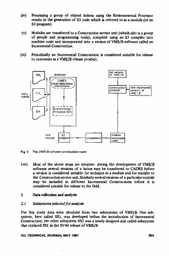
(iv) Processing a group of related holons using the Environmental Processor results in the generation of S3 code which is referred to as a module (or an S3 program).

(v) Modules are transferred to a Construction service unit (which also is a group of people and programming took), compiled using an S3 compiler into machine code and incorporated into a version of VME/B software called an Incremental Construction.

(vi) Periodically an Incremental Construction is considered suitable for release to customers as a VME/B release product.

Fig. 2 The VME/B software production route

(vii) Most of the above steps are iterative: during the development of VME/B software several versions of a holon may be transferred to CADES before a version is considered suitable for inclusion in a module and for transfer to the Construction service unit. Similarly several versions of a particular module may be included in different Incremental Constructions before it is considered suitable for release to the field.

2 Data collection and analysis

2.1 Subsystems selected for analysis

For this study data were obtained from two subsystems of VME/B. One subsystem, here called SSI, was developed before the introduction of Incremental Construction; the other subsystem SS2 was a newly designed and coded subsystem that replaced SSI in the SV40 release of VME/B.


The selection of SSI and SS2 for analysis hinged on several factors. First, they were both fairly small subsystems and therefore it was possible to analyse them without too much effort. Second, they represented extremes of VME/B code in terms of age and the availability of software development aids. Last, since the subsystems had the same basic function, differences between them could not be attributed to different functional requirements.

SSI is composed of 27 modules compiled from a total of 47 holons; some modules were a composite of several different holons. SS2 is composed of 41 modules compiled from a total of 45 holons. Both sets of modules also contained expanded code from other VME/B subsystems obtained by the facility of macro expansion. Three holons of SS2 were macros, none of the SSI holons were macros. One of the SS2 modules was a ‘data-only’ module used to hold information about all the global data required by the subsystem. The data-only module contained no S3 code and was therefore excluded from all analyses. From now on the SS2 subsystem will be considered to be composed of 40 modules compiled from 44 holons. This procedure will not influence the analysis because Halstead excludes declarations from his operator and operand counts.

2.2 Information obtained

The S3 compilation listings, provided by the S3 compiler, were obtained for the 27 modules in SSI and for the 40 code modules in SS2. From these the following metrics were obtained for each module:

(i) — (iv) Halstead’s metrics n i , n 2, N lt N 2 as defined in Section 1.2.

(v) McCabe’s cyclomatic complexity measure V(G) as defined in Section 1.3.

(vi) Number of machine code instructions (Primitive Level Instructions, PLI) in the compiled code.

In order to investigate the efficiency of the various metrics, some observable indicator of program behaviour which could be related to complexity was required. A measure such as the number of bugs per module would have been ideal but suitable records were not available. What was readily available was information collected during the automated stages of holon and module development. Thus it was possible to obtain a count of the number of different versions of each holon processed by CADES during the development of both SSI and SS2 and also of the number of different versions of each module processed by Construction for SS2. Versions of modules and holons are changed for a variety of reasons including error clearance, enhancement, design change and so on. However, on the assumption that a complex program (module or holon) would require more attempts before it was acceptable than a simple program, measures of behaviour based on observed numbers of changes were constructed.

Two measures of module behaviour were obtained, one based on the observed changes to the constituent holons and the other related to the observed changes to each module during Incremental development, thus:


(vii) Number of transfers to CADES (TC). This was derived from the observed changes to the constituent holons of a module. In order to avoid biasing the results because of the different numbers of holons in different modules, the following procedure was adopted: the initial transfer of all the holons comprising a module gave a TC count of one and thereafter the count was increased by one every time a new version of a holon was transferred. Thus a module of five holons, none of which was changed after the initial transfer, would have a TC value of one, whereas a module of two holons, one of which was altered four times after the initial transfer, would have a TC value of five. Any effects of macros were ignored in this procedure.

(viii) Number of transfers to Construction. This was a simple count of the number of different versions of the module that existed in Incremental versions of VME/B during module development. It was available for the modules comprising SS2 but not for SSI which was written before the introduction of Incremental development.

2.3 Statistical analyses

The data were analysed using the 2900 Statistics System11. The additional Halstead metrics described in Section 1.2 were calculated for each module. The statistical analyses were performed on each subsystem separately to provide the following information:

(i) The mean and standard deviation for each metric.

(ii) The frequency histogram of each metric.

(iii) The correlations between the measures of module complexity and the measures of module behaviour defined in Section 2.2.

(iv) The partial correlations between the measures of complexity and the measures of module behaviour using the PLI count as the partial control variate.

(v) The percentage of variation accounted for by fitting each of two linear regression models relating complexity metrics to module behaviour measurements.

a(vi) The program length N plotted against its estimator N.

The limitations of any exploratory study12 apply to this investigation. Two particular points require consideration. First, there is a bias towards finding a general difference between the two subsystems because they were written and coded by different people at different times. Second, although statistical techniques are used to present the information in concise form, reliance on statistical tests of significance is not appropriate because these rely heavily on the Gaussian (Normal) distribution and, as the following Tables will show, the metrics used here are not distributed in this way. However, it was believed that the investigation would provide useful information concerning gross trends and suitable background information in the event of a more rigorous investigation being required.


3 Results

3.1 A verage values o f the metrics

The mean values for each metric together with their standard deviations are shown in Table 1 for SSI and Table 2 for SS2. The striking feature of these two Tables is the similarity observed between complexity metrics for the two subsystems.

Table 1 shows two values for the SSI subsystem. One value includes all 27 SSI modules, the other excludes one module that had extremely large values for all complexity metrics except program vocabulary. This module was considered atypical not simply because of its large values but because the large values were obtained as a result of a large number of macro expansions of a different subsystem. Thus, the complexity measures for that module were inflated as a result of the complexity and method of implementation (macros as opposed to procedures) of an unrelated subsystem.

Table 1. Mean and standard deviation o f measurements obtained from the 27 modules in the SSI subsystem

Measurement Mean* Standard deviation*

Halstead’s metrics

n 80-9 (79-6) 50-4 (50-8)N 426-5 (340-3) 554-9 (334-3)V 2909-4 (2316-5) 3970-6 (2554-8)E 390840-9 (202818-6) 1031224-6 (336551-4)L 0.059 (0-061) 0.115 (0-117)X 1-23 (1-27) 1-00 (1-00)N 459-3 (450-2) 349-5 (351-1)

McCabe’s metric

V(G) 21-4 (19-3) 21-6 (18-9)

Size

Number of PLI 334-7 (295-5) 381-2 (328-6)

Behaviouralmeasurements

Transfers to CADES 5-2 5-1

* The measurements in brackets indicate the values obtained by excluding an atypical module.

Once the atypical module is removed from the analysis, it is apparent that not only are the mean values of the metrics similar but the variability, as demonstrated by the standard deviation, is very similar for each metric within each subsystem.


The individual operator and operand counts are not shown in the Tables because they are treated by Halstead merely as building blocks for his other metrics.

Table 2. Mean and standard deviation of measurements obtained from 40 modules in the SS2 subsystem

Measurement Mean Standard deviation

Halstead’s metrics

n 81-5 48-8N 355-3 326-3V 2417-5 2436-3E 225840-3 392994-6i 0-067 0-130\ 1-20 1-18N 461-5 337-0

McCabe’s metric

V(G) 20-1 19-1

Size

Number of PLI 263-0 236-4

Behaviouralmeasurements

Transfers to CADES 3-05 2-31

Transfers to Construction 2-05 1-08

3.2 Distribution o f the metrics

Examination of the frequency histograms for each complexity metric revealed two points. First, the distributions of the metrics were not normal. Second, the distributions again showed a high degree of similarity between the two subsystems.

To illustrate these two features Fig. 3a, b and c show the frequency histograms for program vocabulary, n, the cyclomatic complexity, V(GJ, and the PLI count for SSI. Fig. 3d, e and / show the equivalent histograms for SS2. (These particular histograms were chosen simply because they provide a representative set of the results.) The class boundaries for each histogram were calculated from the mean and standard deviation of each metric and therefore differ between the two subsystems.

3.3 Correlations between the complexity metrics and the module behaviour

Table 3 shows the correlations between the measures of module behaviour and the complexity metrics for each subsystem.


It is clear that all the complexity metrics, except those related to the language used (i.e. L and X), show consistently large positive correlations with the measures of behaviour, although the correlations observed for SSI are dependent upon the exclusion of the atypical module.

class boundaries

class boundaries

Fig. 3 a Frequency histogram for program vocabulary n of modules in SS1b Frequency histogram for cyclomatic complexity V(G) o f modules in SSI c Frequency histogram for PLI count of modules in SSId Frequency histogram for program vocabulary n of modules in SS2e Frequency histogram for cyclomatic complexity l/ (G) of modules in SS2 f Frequency histogram for PLI count of modules in SS2

The results, therefore, indicate that the most frequently modified modules (which may be considered the badly-behaved modules) are those which exhibit the larger values of the complexity metrics. There is also a weak indication that modules with a high level of abstraction are less frequently amended (well-behaved).

The complexity metrics were highly correlated among themselves as can be seen in Tables 4 and 5 for SSI and SS2 subsystems, respectively. (The results for SSI, shown in Table 4, are given for the 26 normal modules only.) The correlations are


extremely consistent in pattern between the two subsystems. All the straightforward complexity metrics are highly positively correlated, while the two different metrics, language level (X) and level o f abstraction (£,), are only moderately and negatively correlated with the other metrics although highly correlated with each other.

Table 3. Correlations between the complexity metrics and module behaviour measurements for SSI and SS2

Transfers toComplexity metrics Transfer to CADES Construction

SSI modules* SS2 modules S2 modules

(a) Halstead's

n 0-74 (0-75) 0-72 0-64X 0-45 (0-77) 0-70 0-51N 0-76 (0-77) 0-73 0-64V 0-48 (0-78) 0-70 0-51E 0-26 (0-83) 0-53 0-32L -0-28 (-0-28) -0-34 -0-36X -0-40 (-0-41) -0-38 -0-39

(b) McCabe’s

V(GJ 0-68 (0-79) 0-70 0-46

(c) Size

PLI 0-66 (0-80) 0-72 0-51

*The bracketed values are those obtained when the atypical module is excluded from the analysis.

N.B. For pairs of bivariate normal random variables, a value of the correlation coefficient significant at the 0-01 level is 0-50 for 26 observations and 0-40 for 40 observations.

The high positive correlations between the complexity measures indicate a potential problem, in that they may all be measuring the same thing. For this reason, the partial correlations between the complexity measures and the behavioural measures were investigated. The PLI count was chosen to be the control variable for two reasons: the simplest hypothesis is to suggest that all the complexity metrics are related to size and, for future use, the PLI count is the simplest metric to obtain, since it is provided by the S3 compiler.

The partial correlations between the complexity metrics and the module behaviour measurements using PLI as the partial control variable are shown in Table 6. The partial correlations indicate the relationships between the complexity metrics and module behaviour for fixed module size.

It can be seen that the correlations are no longer consistent between the two subsystems nor do they show any consistent trends within the subsystems. Most of the correlations are now negligible, and the few that remain moderately large are not confined to one subsystem or one metric.


Table 4 . Correlations between the compexity metrics for the SSI subsystem*

Halstead’s metrics McCabe’s

V(G)

Size

PLIn NA

N V EAL A

n _N 0-94 -

N 100 0-96 _

V 0-94 1-00 0-96 —

E 0-88 0-97 0-91 0-98 _

L -0-52 -0-39 -0-46 -0-36 -0-27 —

X -0-59 -0-48 -0-55 -0-47 -0-41 0-75 _

V(G) 0-85 0-84 0-86 0-83 0-82 -0-38 -0-51 —

PLI 0-91 0-99 0-93 0-99 0-92 -0-35 -0-47 0-93 —

4The correlations in this Table are based on the 26 normal modules

Table 5. Correlations between the complexity metrics for the SS2 subsystem

Halstead’s metrics McCabe’s

V(G)

Size

PLIn NA

N V EAL X

n _

N 0-91 —

N 1-00 0-92 _

V 0-92 0-93 0-93 —

E 0-73 0-74 0-74 0-73 -L -0-57 -0-51 -0-40 -0-57 -0-25 _X -0-61 -0-56 -0-56 -0-61 -0-34 0-83 -

V(G) 0-83 0-92 0-94 0-93 0-86 -0-40 -0-45 -

PLI 0-93 0-93 0-93 0-99 0-89 -0-44 -0-51 0-94 -

Because partial correlations are not guaranteed robust to the effects of non-normality, these results were verified Jpy investigating the effects of fitting a number of regression models. The metrics L and X were excluded from this analysis since they are measures of language rather than program complexity. Two types of regression model were used, as follows:

y = b0 + b lXl (Model 1)

y = bo + b\X\ + Z?2*X2 (Model 2)

For the first model, each complexity metric was used in turn as the independent variable, xj, and the module behaviour measurements (transfers to CADES and transfers to Construction) were taken in turn as the dependent variable y. The subsystems SSI and SS2 were analysed separately. Each model was summarised by the percentage of variance of the dependent variable y accounted for by fitting the


regression model, where the higher the percentage of variance accounted for the better model.

For the second model, a similar analysis was performed except that the first independent variable, x 2, was always taken to be the number of PLI while the other complexity measures were taken in turn as the second independent variable, x 2. Each model was, again, summarised by the percentage of variance accounted for by fitting the regression model.

Table 6. Partial correlations between the complexity metrics and module behaviour measurements using PLI as the partial control variable

Transfers to CADES Transfers toComplexity metrics ------------------------------------------------- Construction

SSI modules* SS2 modules SS2 modules

(a) Halstead’s

n 0-46 (0-14) 0-18 0-51% -0-57 (-0-10) -0-17 -0-01N 0-49 (0-15) 0-21 0-52V -0-56 (-0-04) -0-15 -0-01E -0-08 (0-51) -0-37 -0-37L -0-56 (0-00) -0-04 -0-12\ -0-11 (-0-07) -0-02 -0-12

(b) McCabe’s

V(G) 0-28 (0-42) 006 -0-08

♦The bracketed values are those obtained when the atypical module is excluded from the analysis.

The results of applying both models to the two subsystems when using transfers to CADES as the dependent variable (y) are shown in Table 7. The results of applying both to SS2 when using transfers to Construction as the dependent variable are shown in Table 8.

It is apparent from Table 7 that when transfers to CADES is used as the measure of module behaviour, the results for Model 1 suggest that using PLI as independent variable is usually as good as using any other metric; and that no other is consistently better. Inspection of the results for Model 2 shows that in general only a very modest improvement over the Model 1 results for PLI alone can be expected from introducing a combination of PLI and another metric.

When transfers to Construction is used as the measure of module behaviour, the results shown in Table 8 indicate that Halstead’s vocabulary metric n and estimated size metric N appear to be better predictors of module behaviour than PLI, using Model 1. However, the results for PLI are similar to those for most of the other metrics and are substantially better than Halstead’s ‘mental effort’ metric E. The


results of using Model 2 show that, apart from the combination of PLI and E, combining PLI with any other metric does not provide a substantial improvement over Model 1.

Considering the correlation and regression analyses together, it appears that PLI is a fairly good and consistent indicator of module behaviour although other metrics may be better for specific cases. In general therefore most of the complexity metrics cannot be shown to provide information in excess of that provided by the PLI count.

Table 7. Percentage o f variation accounted for by regression models using transfers to CADES as the dependent variable

Independent variates SSI SS2

Complexity Model 1* Model 2* Model 1 Model 2metrics

(a) Halstead’s

n 51-7 541 56-6 62-8N 48-4 53-7 59-4 62-3A

N 53-0 54-6 58-5 63-0V 48-8 53-5 60-5 62-0E 28-2 59-0 69-6 72-0

(b) McCabe’s

V(G) 48-5 52-6 62-9 68-8

(c) Size

PLI 52-4 - 62-0 -

* Model 1 isy = bo + b tx t

Model 2 is y - bo + 6 1*1 + b2x2 where x l is PLI.

3.4 Relationship between N and N

As mentioned in Section 1.2, Halstead proposed an estimator of program length based only on the number of distinct operators and operands (eqn. 3). The correlations in Tables 4 and 5 indicate that N and N are very closely related to one another (0-96 for SSI, 0-92 for SS2). However, it is not clear from correlations whether or not an identity relationship holds.

Figs. 4 and 5 demonstrate the nature of the relationship between N and N observed in this investigation. It is clear that the relationship N = N is not a good fit to the observed data for either subsystem. Both subsystems show the same trend which is for N to over-estimate N.


Table 8. Percentage of variation accounted for by regression models using transfers to Construction as the dependent variable

Independent variates SS2

Complexity metrics Model 1* Model 2*

(a) Halstead’sn 41-2 45-8H 25-6 26-5N 40-9 46-1V 25-8 26-5E 1 0 0 36-7

(b) McCabe’sF(G) 21-6 26-9

(c) SizePLI 26-5 -

♦Model 1 is y = bo + bix l Model 2 isy = b0 + b lx 1 + 62*2 where is PLI.

4 Discussion

4.1 Distributions o f the complexity metrics

The most striking feature of the distributions of the complexity metrics is the similarity observed between the two subsystems. The similarity exists not only for average values but also for standard deviation and frequency histograms.

The similarity is surprising for two reasons. First, there was almost certainly a bias in favour of finding a difference (see Section 2.3). Second, the subjective opinion of programmers responsible for maintaining the subsystems is that SSI is more complex than SS2.

Fig. 4 a Relationship between length N of a module and proposed estimator N, for modules in SS1

b Relationship between length N of a module and proposed estimator N, for modules in SS2


A possible explanation is that this phenomenon is another example of the influence of program size. One feature of the software design, common to the development of both subsystems, was the requirement to constrain holon size. Now, the average PLI count is similar for each subsystem, indicating that the size constraint has influenced module size as well as holon size. It is therefore possible that the similar distributions of the Halstead and McCabe metrics have occurred because the metrics themselves are highly correlated with PLI count.

4.2 McCabe’s complexity metric

This measure of complexity has a good deal of intuitive appeal, when viewed in terms of a measure of the number of paths through a program. Although it is obvious that there must be a gross relationship between the size of a program and the number of paths through it, it is surprising that this measure of complexity offered little or no additional information to the ranking of programs.

McCabe7 applied his work to application programs written in FORTRAN and concluded that a cyclomatic complexity number of 10 should be considered as a practical upper limit for software modules. The average value obtained from both subsystems investigated in this study was 20. It may be that above a certain level of complexity McCabe’s metric is unable to discriminate between programs, and that the only conclusion to be drawn is that VME/B software written in S3 is extremely complex.

4.3 Halstead’s metrics

Halstead’s metrics have less intuitive appeal than McCabe’s metric because they are derived metrics. However, Halstead6 has provided a detailed justification of them and the reported results have usually confirmed their usefulness.

Two features concerning the internal consistency of Halstead’s metrics can be found in this study. First, the language level for S3 was estimated as 1-23 for SSI and 1-20 for SS2. In view of the high level of S3, and compared with the values of 1-21 for Algol 58, 1-14 for FORTRAN and 1-53 for PL/1 which have been reported,4’13 a language level of approximately 1 -2 seems rather low.

Second, the relationship between the observed program length N and the estimated program lengtji N predicted by Halstead does not appear to hold for the modules studied here. A is highly correlated with N but overestimates N. Halstead has indicated a number of reasons why N should fail to estimate N accurately. However, there is no suggestion in his work of a systematic deviation from the proposed relationship which could explain the results observed in this study.

4.4 Relationship between complexity metrics and measures o f module behaviour

McCabe’s metric, all Halstead’s metrics (with the exception of Language Level and Level of Abstraction) and PLI count show moderate to high correlation with the measures of module behaviour (transfers to CADES and transfers to Construction).


However, the metrics themselves and the relationships were very susceptible to the values obtained for one atypical module.

The partial correlation and regression analyses suggest that in most cases neither McCabe’s nor Halstead’s metrics offer much additional information over and above that to be obtained from the F LI count. It was found that Halstead’s vocabulary metric n and estimator of size N were better than PIT as estimators of the numbers of transfers to Constructions of SS2 modules. However, the good results for these two metrics are unexpected in terms of Halstead’s own theories: he does not regard vocabulary as a basic complexity measure, but as more of a building block for other metrics. The result for N is even more unlikely, since this is supposed to be an estimator for program size N and is therefore expected to behave in a similar way to N; but in this case N is apparently a better predictor of module behaviour than N itself.

5 Conclusions

This investigation has confirmed that module size is a good measure of program complexity and a reasonable indicator of subsequent module behaviour for VME/B modules.

It also seems clear that McCabe’s and Halstead’s metrics offer little assistance to the evaluation of VME/B modules or subsystems beyond that obtained by considering module size. In addition, it is worth noting that McCabe’s and Halstead’s metrics are extremely arduous to obtain compared with PLI count, which restricts their usefulness in practice.

The results of this study also cast some doubts on the generality of Halstead’s and McCabe’s metrics. This is in contrast to much of the previously published work summarised by Fitzsimmons and Love13 , but is similar to the results of Curtis et al8, which also observed strong correlations between program size and McCabe’s and Halstead’s metrics. Now, the research — both theoretical and empirical — relating to the McCabe and Halstead metrics is of far too comprehensive a nature to be ignored. The results of this study would therefore seem to suggest that more research is required to identify the particular conditions under which these metrics are of practical use.

Acknowledgments

The author would like to thank Dr. R.A. Snowdon and Mr. B.C. Pearson for their constructive comments concerning the presentation of the material in this paper. She is also extremely grateful to Mrs. C. Lodge for her help with the preparation of the manuscript.

References

1 DUKSTRA, E.W.: ‘The Structure of the “THE” - Multiprogramming System’, Commun. ACM, 1968,11(5), 341-346.

2 PARNAS, D.L.: ‘On the criteria to be used in decomposing systems into modules’, Commun. ACM, 1972,15(12), 1053-1058.


3 WIRTH.N.: ‘Program development by stepwise refinement’, Commun. ACM, 1971, 14(4), 221-227.

4 LEHMAN, M.M.: ‘Laws of program evolution - rules and tools for programming management’, in Why software projects fail, Infotech State of the Art Conference, 1978, 11/3- 11/25.

5 KOLENCE, K.W.: ‘Software physics’, Datamation, 1975, June, 48-51.6 HALSTEAD, M.H.: Elements o f software science, Elsevier North-Holland Inc. N.Y., 1977.7 McCABE, T.J.: ‘A complexity measure’, IEEE Trans. Software Eng., 1976, SE-2(4),

308-320.8 CURTIS, B., SHEPPARD, S.B., MILL1MAN, P., BORST, M.A. and LOVE, T.: ‘Measuring

the psychological complexity of software maintenance tasks with the Halstead and McCabe metrics’, IEEE Trans. Software Eng., 1979, SE-5(2), 96-104.

9 GORDON, R.: ‘Measuring improvements in program clarity’, IEEE Trans. Software Eng., 1979, SE-5(2), 79-90.

10 McGUFFIN, R.W., ELLISTON, A.E., TRANTOR, B.R. and WESTMACOTT, P.N.: ‘CADES - software engineering in practice’, ICL Tech. /., 1980 2(1), 13-28.

11 COOPER, B.E.: ‘Statistical and related systems’, ICL Tech. /., 1979, 1(3), 229-246.12 CAMPBELL, D.T. and STANLEY, J.C.: Experimental and quasi-experimental designs for

research, Rand McNally College Publishing Co., Chicago, 1966.13 FITZSIMMONS, A. and LOVE.T.: ‘A review and evaluation of software science’, Comput.

Surv., 1978, 10(1), 3-18.


icl technical journal volume 2 issue 3 - may 1981 board welcomes mr. davies with this issue of the...

Documents