i 11111 1llllll1111 lllll 11111 11111 11111 ill11 11111 ... 11111 1llllll1111 lllll 11111 11111...

I 11111 1llllll1111 lllll 11111 11111 11111 Ill11 11111 11111 Ill11 llllll111 Ill11 Ill1 US0054287 10A

United States Patent [I91 [11] Patent Number: 5,428,718 Toomarian et al. [45] Date of Patent: Jun. 27, 31995

FAST TEMPORAL NEURAL LEARNING USING TEACHER FORCING

Inventors: Nikzad Toomarian, Encino; Jacob

Assignee:

Barhen, La Crescenta, both of Calif.

The United States of America as represented by the Administrator of the National Aeronautics and Space Administration, Washington, D.C.

Appl. No.: 908,677

Filed: Jun. 29,1992

Int. C1.6 .............................................. G06F 15/18 U.S. C1. ........................................ 395/23; 395/20;

395/21 Field of Search ....................... 395/21, 22, 23, 11,

395/27; 382/15

References Cited U.S. PATENT DOCUMENTS

4,804,250 2/1989 4,912,652 3/1990 4,918,618 4/1990 4,926,064 5/1990 4,951,239 8/1990 4,953,099 8/1990 4,967,369 10/1990 4,990,838 2/1991 5,014,219 5/1991 5,046,019 9/1991 5,046,020 9/1991 5,050,095 9/1991 5,052,043 9/1991 5,056,037 10/1991 5,058,034 10/1991 5,075,868 12/1991 5,086,479 2/1992 5,093,899 3/1992 5,146,602 9/1992 5,253,329 10/1993 5,313,558 5/1994

Johnson .......................... 330/162.12 Wood .................................. 364/513 Tomlinson, Jr. .................... 364/513

Jourjine ............................... 364/513 Jourjine ............................... 364/513 Kawato et al. ................ 318/568.10

.......................... 395/23 Basehore ............................. 364/513

Samad ................................. 364/513 Gaborski ............................... 382/14 Eberhardt ............................. 395/23 Murphy et al. ....................... 395/23 Andes et al. .......................... 395/23 Takenaga et al. .................... 382/14 Hiraiwa ................................. 395/23 Holler et al. .......................... 395/23 Villarreal et al. ..................... 395/23 Adams .................................. 395/22

OTHER PUBLICATIONS Michail Zak, “Terminal Attractors in Neural Net- works,” Neural Networks, vol. 2, pp. 259-274, 1989. J. Barhen, et al., “Application of Adjoint Operators to

~)an(tyPen(t)Pmnu.

Neural Learning”, Aool. Math. Lett., vol. 3 No. 3, pp. 13-18, 1990 Printed in Great Britain. J. Barhen, et al., “Adjoint Operator Algorithms for Faster Learning Dynamical Neural Networks”, Center for Space Micro-electronics Technology, Jet Propul- sion Laboratory, California Institute of Technology,

R. J. Williams et al., “A Learning Algorithm for continually running fully recurrent neural networks,” Neural Computation, vol. 1, No. 2 pp. 270-280.

(List continued on next page.)

pp. 498-508.

Primary Examiner-Robert W. Downs Assistant Examiner-Tariq R. Nafiz Attorney, Agent, or Firm-John H. Kusmiss; Thomas H. Jones; Guy M. Miller

[571 ABSTRACT A neural network is trained to output a time dependent target vector defined over a predetermined time interval in response to a time dependent input vector defined over the same time interval by applying corresponding elements of the error vector, or difference between the target vector and the actual neuron output vector, to the inputs of corresponding output neurons of the network corrective feedback. This feedback decreases the error and quickens the learning process, so that a much smaller number of training cycles are required to complete the learning process. A conventional gradient descent algorithm is employed to update the neural network parameters at the end of the predetermined time interval. The foregoing process is repeated in repetitive cycles until the actual output vector corresponds to the target vector. In the preferred embodiment, as the overall error of the neutral network output decreases during successive training cycles, the portion of the error fed back to the output neurons is decreased accordingly, allowing the network to learn with greater freedom from teacher forcing as the network parame-

’ ters converge to their optimum values. The invention may also be used to train a neural network with station- ary training and target vectors.

-

39 Claims, 10 Drawing Sheets

https://ntrs.nasa.gov/search.jsp?R=19960009260 2018-06-25T19:36:17+00:00Z

5,428,710

OTHER PUBLICATIONS

R. J. Williams et al., “A Learning Algorithm for continually running fully recurrent neural networks,” Techni- cal Report ICs Report 8805, UCSD, La Jolla, Califor- nia 92093. Kumpati S . Narendra fellow, IEE and Kannan Par- thasarathy, “Identification and Control of Dynamical Systems Using Neural Networks”, vol. 1 No. 1, Mar. 1990. Masa-aki Sato, “A Learning Algorithm to Teach Spa- tiotemporal Patterns to Recurrent Neural Networks”, Biological Cybernetics, (1990) pp. 259-263. Masa-aki Sato, “A Real Time Learning Algorithm for Recurrent Analog Neural Networks”, Biological Cy- bernetics, (1990) pp. 237-241. Fernando J. Pineda, “Time Dependent Adaptive Neu- ral Networks”, Center for Microelectronics Technol-

ogy, Jet Propulsion Laboratory, California Institute of Technology, pp. 710-718. N. Toomarian and J. Barhen, “Adjoint-Operators and Non-Adiabatic Learning Algorithms in Neural Net- works”, Appl. Math. Lett., vol. 4 No. 2, pp. 69-73, 1991, printed in Great Britain. Barak A. Pearlmutter, “Dynamic Recurrent Neural Networks”, School of Computer Science, Carnegie Mellon University, Pittsburgh, Pa. 15213. This research was sponsored in part by The Defense Advanced Re- search Projects Agency, Information Science and Technology Office, under the title Research on Parral- le1 Computing, ARPA Order No. 7330 issued by DAR- PA/CMO. Barak A. Pearlmutter, “Learning State Space Trajecto- ries in Recurrent Neural Networks”, Neural Computa- tion 1, pp. 263-269 (1989) Massachusetts Institute of Technology.

U.S. Patent

I- -

June 27, 1995 Sheet 1 of 10

4

- 4 - I I cn

0

0

0

0

I 0

U.S. Patent June 27, 1995 Sheet 2 of 10

6

FIG. 2 (PRIOR ART)

“t 4- I 1

FIG. 4

US. Patent June 27, 1995

AMPLITUDE

AMPLITUDE

Sheet 3 of 10

c

FIG. 3

U'n ( t+dt )

FIG.

US. Patent June 27, 1995 Sheet 4 of IO 5,42

U.S. Patent June 27, 1995 Sheet 5 of 98 5,428,71

DEFINE NEURON TEMPORAL LEARNING BEHAMOR FOR M NRWORK PARAMRERS T & , p K j , Y i 30

il

32

INPUT anw TO INPUT NEURONS

f- 38 OBSERVE ERRORS e&)

c PERFORM GRADIENT DESCERT ALGORITHM

FOR EACH OF THE M NETWORK PERAMETERS

40 J

US. Patent June 27, 1995 Sheet 6 of 1Q


DEFINE NEURON TEMPORAL LEARNING BEHAVIOR FOR M NETWORK PARAMETERS ~ ~ , p K j l ” Y ~

~

DEflNE TRAINING SET:

an(t) FOR n IN O :OUTPUT PAITEXN FOR n IN I ANPUT PATERN

FOR TIME INTERVAL t o T

FIG. 9a


FROM THE TEMPORAL LEARNING BEHAVIOR

~ r r , r + & ~ n , m ~ r n , p = ~ n . g

SOLVE THE FORWARD SENSITIWIY EQUATIONS M TIMES , ONCE FOR EACH OF THE M NRWORK

PARAMEl'ERS FOR -pp

40 c

42

FIG. 9 b

U.S, Patent June 27, 1995 Sheet 9 of 10

0.6 I

-0.6 0.0 0.6

FIG. 10

0.6 1 f

0.0

-0.6 -0.6 0.0 0.6

FIG. 12

0.0

-0.6

e

4

3 z g 2 w

1

0

LEARN I N G BTERATIO NS

US. Patent June 27, 1995 Sheet 10 of 18

0.6 1

1 0.0

-0.6 I I

-0.6 0.0 0.6

FIG. 14

0.0

-0.6 -0.6 0.0 0.6

FIG. 16

5

4

u 3 0 K

5 2

1

0

0.6

0.0

-0.6 -0.6 .o

0 200 400 600 800 100 LEARNING ITERAVIONS

5,428,710 1

FAST TEMPORAL NEURAL LEARNING USING TEACHER FORCING

BACKGROUND OF THE INVENTION 5

Origin of the Invention The invention described herein was made in the per-

formance of work under a NASA contract, and is sub- ject to the provisions of Public Law 96-517 (35 USC 10 202) in which the contractor has elected not to retain title.

Technical Field

with time dependent phenomena and to the problems associated therewith, including reducing the number of computations required and increasing the quality or fidelity of the neural network output.

Background Art

The invention relates to training neural networks 15

20

Recently, there has been a tremendous interest in developing learning algorithms capable of modeling time-dependent phenomena. In particular, considerable attention has been devoted to capturing the dynamics embedded in observed temporal sequences.

In general, the neural architectures under consider- ation may be classified into two categories:

* Feedforward networks, in which back propagation through time can be implemented. This architecture has been extensively analyzed, and is widely used in simple applications due, in particular, to the straightforward nature of its formalism.

* Recurrent networks, also referred to as feedback or fully connected networks, which are currently receiving increased attention. A key advantage of recurrent networks lies in their ability to use information about past events for current computations. Thus, they can provide time-dependent outputs for both time-dependent as well as time-independent inputs.

One may argue that, for many real world applications, the feedforward networks suffice. Furthermore, a recurrent network can, in principle, be unfolded into a multilayer feedforward network. A detailed analysis of the merits and demerits of these two architectures is beyond the scope of this specification. Here, we will focus only on recurrent networks.

The problem of temporal learning can typically be formulated as a minimization, over an arbitrary but finite time interval, of an appropriate error functional. The gradients of the functional with respect to the various parameters of the neural architecture, e.g., synaptic weights, neural gains, etc. are essential elements of the minimization process and, in the past, major efforts have been devoted to the efficacy of their computation. Calculating the gradients of a system’s output with respect to different parameters of the system is, in general, of relevance to several disciplines. Hence, a variety of methods have been proposed in the literature for computing such gradients. A recent survey of techniques which have been considered specifically for temporal learning can be found in Pearlmutter, B. A. (1990) “Dynamic recurrent neural networks,” Techni- cal Report CMU-CS-90-196, School of Computer Sci- ence, Carnegie Mellon University, Pittsburgh, Pa. We will briefly mention only those which are relevant to the oresent invention.

25

30

35

40

45

50

55

60

65

Sat0 proposed, at the conceptual level, an algorithm based upon Lagrange multipliers. However, his algorithm has not yet been validated by numerical simulations, nor has its computational complexity been analyzed. Williams and Zipset [Williams, R. J., and Zipser, D. (1989) “A learning algorithm for continually running fully recurrent neural networks”, Neural Computation, Vol. 1, No. 2, pp. 270-2801 presented a scheme in which the gradients of an error functional with respect to network parameters are calculated by direct differentia- tion of the neural activation dynamics. This approach is computationally very expensive and scales poorly to large systems. The inherent advantage of the scheme is the small storage capacity required, which scales as O(N3), where N denotes the size of the network.

Pearlmutter, on the other hand, described a varia- tional method which yields a set of linear ordinary differential equations for backpropagating the error through the system. These equations, however, need to be solved backwards in time, and require temporal storage of variables from the network activation dynamics, thereby reducing the attractiveness of the algorithm. Recently, the inventors herein [Toomarian, N. and Bar- hen, J. (199 1) “Adjoint operators and non-adiabatic algorithms in neural networks,” Applied Mathematical Letters, Vol. 4, No. 2, pp. 69-73] suggested a framework formalism which enables the error propagation system of equations to be solved forward in time, con- comitantly with the neural activation dynamics. A drawback of this novel approach came from the fact that their equations had to be analyzed in terms of distri- butions, which precluded straightforward numerical implementation. Finally, Pineda proposed combining the existence of disparate time scales with a heuristic gradient computation. The underlying adiabatic as- sumptions and highly approximate gradient evaluation technique, however, placed severe limits on the applica- bility of his method.

Analogy to real-life behavior motivates the learning paradigm of the present invention described below. Suppose that a parent wants to teach his child to ride a bicycle. Clearly, the parent will not stay home, let his child ride the bicycle and, from time to time, tell him how good or bad he is performing (just as it happens in classical supervised learning). The best way to train the child would be for the parent to accompany him during the riding sessions. This suggests that different dynamical systems should be considered for the two basic stages of learning and recall (or generalization). How- ever, the functional form of the neural dynamics used during the learning stage should smoothly evolve toward the functional form of the neural dynamics to be used during recall, after training is completed. In this context, the network dynamics during the learning stage should include an instantaneous signal from the teacher on its performance. This necessitates a mechanism for incorporating information regarding the desired output directly into the activation dynamics. Such a mechanism has been referred to as teacher forcing. Williams and Zipset [williams, R. J., and Zipset, D. (1988) “A learning algorithm for continually running fully recurrent neural networks,” Technical Report ICs Report 8805, UCSD, La Jolla, Calif. 920931, to the best of our knowledge, have been the primary users of teacher forcing. They limited their algorithm to a discrete- time problem, replacing the output of the network with desired output values at each time step.

3 5,428,7 10

4 SUMMARY O F THE INVENTION FIGS. 10, 11 12 illustrate different simulation results

of a neural network learning a circular motion using the The present invention is a new continuous form of invention.

teacher forcing, and appropriately modifies the activa- FIG. 13 is a graph of the error as a function of the tion dynamics of a simple additive neural network dur- 5 number of learning iterations for each of the cases illus- ing its learning stage. The temporal modulation of trated in FIGS. 10-12. teacher forcing is analyzed as learning proceeds, so that FIGS. 14, 15 ad 16 illustrate different simulation re- the activation dynamics of the learning stage can m u - sults of a neural network learning a figure-eight motion ally be reduced to the activation dynamics of the recall using the invention. stage. FIG. 17 is a graph of the error as a function of the

In accordance with the invention, a neural network is number of learning iterations for each of the cases illus- trained to output a time dependent target vector defined trated in FIGS. 1&16. over a predetermined time interval in response to a time dependent input vector defined over the same time interval by applying corresponding elements of the l5 error vector, or difference between the target vector and the actual neuron output vector, to the inputs of corresponding output neurons of the network as correc- We formalize a neural network as an adaptive dynam-

quickens the learning process, so that a much smaller 20 the following set of coupled nonlinear differential equa- number of training cycles are required to complete the learning process. The learning process employs a conventional gradient descent algorithm to update the neural network parameters (e.g., synapse weights and/or neuron gains) at the end of the time interval. The foregoing process is repeated in repetitive cycles until the actual output vector corresponds to the target vector. It has been found that not only is the number of required where U n represents the output of the nth neuron (u, (0) training cycles decreased but that the quality or fidelity being the initial state), and Trim, denotes the strength of of the neural network output is significantly increased 30 the synaptic coupling from the m-th to the n-th neuron. by the invention. In the preferred embodiment, as the The constants K n characterize the decay of neuron ac- overall error of the neural network output decreases tivities. The sigmoidal functions &(*) modulate the neu- during successive training cycles, the portion of the ral responses, With gain given by Yn; typically, error fed back to the output neurons is decreased ac- 35 g d Y n x ) = ~ ( P n x ) . In order to implement a ~ ~ n l i n e a r cordingly, allowing the network to learn with greater functional mapping from an NI-dimensional input space freedom from teacher forcing as the network parame- to an Nodimensional output space, the neural network ters converge to their optimum values. is topographically partitioned into three mutually exclu-

sive regions. As shown in FIG. la, the partition refers BRIEF DESCRIPTION OF THE DRAWINGS 4o to a set of input neurons SI, a set of output neurons SO, FIG. l a is a diagram of a neural network of the prior and a set of “hidden” neurons SH. Note that this archi-

tecture i s not formulated in terms of “layers” and that FIG. 16 a diagram of a neural network training archi- each neuron may be connected to all others including

itself. FIG. 2 is a diagram of a neural network numerical 45 Let $t) (the overhead bar denotes a vector) be an N-

dimensional vector of target temporal patterns, with non zero elements, an(t), in the input and output sets only. When trajectories, rather than mappings, are considered, components in the input set may also vanish.

50 Hence, the time- dependent external input term in Eq. (l), i.e., I,(t), encodes component-contribution of the target temporal pattern via the expression

lo

DETAILED DESCRIPTION OF THE INVENTION

Temporal Learning Framework

tive feedback. This feedback decreases the error and ical system whose temporal is governed by

tions:

(1)

i n i- Kn Un = gn [ Yn (: Tnm Urn + I n 25

art.

tecture of the prior art.

training architecture of the prior art including error feedback which nulls the error at each numerical step.

FIG. 3 is a time domain diagram illustrating the behavior of the neural network training architecture of FIG. 2.

FIG. 4 is a simplified diagram of a neural network training architecture embodying the present, invention.

FIG. 5 is a time domain diagram illustrating the behavior of the neural network training architecture of FIG. 4. 55

FIG. 6 is a system diagram corresponding to the neural network training architecture of FIG. 4.

FIG. 7 is a flow diagram illustrating the operation of the neural network training architecture of FIG. 4 using To proceed formally with the development of a tem- a generic gradient descent algorithm for computing the 60 poral learning algorithm, we consider an approach neural network parameter changes during training. based upon the minimization of an error functional, E,

FIG. 8 is a system diagram illustrating a preferred defined over the time interval [to,td by the following embodiment of the system of FIG. 5. expression

FIGS. 9a and 96 together constitute a flow diagram illustrating the operation of the neural network training 65 architecture of FIG. 4 for an embodiment employing a

rithm.

(2) a&) if n PSI

= o i f n e SH u SO

(3) E ( Z 3 = ‘t Z: en2 dt = Fdt J Y particular type of conventional gradient descent algo- to

5,428,710 5

where the error component, en(t), represents the difference between the desired and actual value of the output neurons, i.e.,

(4) an(t) - un(t) if n E So

i f n a S I U SH e&) =

In our model, the internal dynamical parameters of interest are the strengths of the synaptic interconnections, Trim, the characteristic decay constants, un, and the gain parameters, yn, They can be represented as a vector of M [where: M=N*+2N] components

F=)Tii.. . . , TNN, KI,. . . KN, yi . . . . ,YN} (5)

We will assume that the elements of 5 are statistically independent. Furthermore, we will also assume that, for a specific choice of parameters and set of initial conditions, a unique solution of Eq. (1) exists. Hence, the stag variables u are an implicit function of the parameters p. In the rest of this paper, we will denote the pth element of the vector p by pp ( p = 1, . . . , M).

Traditionally, learning algorithms are constructed by invoking Lyapunov stability arguments, i.e., by requir- ing that the error functional be monotonically decreasing during learning time, T. This translates into

One can always choose, with 77 > 0

5

10

15

20

25

30

which implements learning in terms of an inherently local minimization procedure. Attention should be paid to the fact that Eqs. (1) and (7) may operate on different time scales, with parameter adaptation occurring at a slower pace. Integrating the dynamical system, Eq.(7), over the interval [T, ?-+AT], one obtains,

40

Equation (8) implies that, in order to update a system parameter pp, one must evaluate the “sensitivity” (Le., 50 the gradient) of E, Eq. (3), with respect to ppin the interval [T, T + ~ T ] . Furthermore, using Eq. (3) and observing that the time integral and derivative with respect to pp, commute, one can write

55

This sensitivity expression has two parts. The first term 60 in the Right Hand Side (RHS) of Eq.(9) is called the “direct effect”, and corresponds to the explicit depen- dence of the error functional on the system parameters. The second term in the RHS of Eq. (9) is referred to as the “indirect effect”, and corresponds to the implicit 65 relationship between the error functional and the system parameters via u. In our learning formalism, the error functional, as defined by Eq. (3), does not depend

6 explicitly on the system parameters; therefore, the “direct effect” vanishes, i.e.,

Since F is known analytically (viz. Eqs. (3) and (4)), computation of J F h u is straightforward. Indeed

Thus, to enable evaluation of the error gradient using Eq. (9), the “indirect effect” matrix should, in principle, be computed.

TEACHER FORCING The neural activation dynamics specified by Eqs. (1)

and (2) does not include explicit information regarding the desired network output. If these equations are used in conjunction with the learning formalism described in the previous section, the network parameters (Le., the elements of i) will be modified at the end of a trajectory, i.e., at time t j as shown schematically in FIG. lb . Such a parameter adaptation is based upon the total error between the desired and the actual output of the network, accumulated over the interval [to,tf3. Refer- ring to FIG. lb, a neural network 2 is stimulated by a time-varying training vector I(t) to produce a time- varying output vector u(t). A subtractor 4 subtracts the output vector u(t) from a time-varying target vector a(t) to produce a time-varying error vector e(t). An integrator 6 integrates the error vector e(t) over the time period of the time-varying training vector I(t). At the end of the time period, the result of this integration is used by a gradient descent algorithm to change the parameters (e.g., the synapse weights) of the neural network in such a manner as to reduce the output of the integrator 6 in the next time period. In our earlier analogy to real- life behavior, this would correspond to a parent staying home, letting his child ride a bicycle and, after each trial, telling him all the errors he made. “Conventional” supervised learning operates in this fashion, and usually takes a great deal of iterations to produce the desired results.

In order to overcome this difficulty, we consider the concept of teacher forcing, Le., driving the output neurons to desired values in finite time. Williams and Zipser williams, R. J., and Zipser,’D. (1988) “A learning algorithm for continually running fully recurrent neural networks,” Technical Report ICs Report 8805, UCSD, La Jolla, Calif. 920931 disclose forcing in a similar context. Their focus, however, is on discrete time problems. To highlight the differences between the two ap- proaches we make the following observations. By defi- nition, the conventional output of a network at time step (t+l), without teacher forcing, is a function of the external inputs to the network and of the networks’- states at time step (t), i.e., in our notation, M+ 1)=gn[W,u~4,Pl

where n&o, ieSI and JcSIUSHUSo. T o introduce teacher forcing, Williams and Zipser replace the output of the network with the desired output values at time step (t). This means that

un(t+ ~ ) = g n [ ~ ~ ~ r ) , ~ ~ r ) . ~ n C r ) m

5,428,710 7 8

N. and Gulati, S. (1990) “Adjoint operator algorithms where ncSo, icSI and j c S N SH. The network parame- for faster learning in dynamical neural networks,” in ters can be updated either at the end of each time step, David S . Touretzky (Ed.), Advances in Neural Informa- or at the end of the trajectory, i.e., at time tr. A sche- tion Processing Systems, Vol. 2, pp. 498-508, San Mateo, matic block diagram of this model, in which the param- 5 calif. (Morgan Kaufmm); and, Barhen, J., Toomanan, eters are updated at the end of the trajectory, is given in N. and Gulati, S. (1990) ‘‘Application of adjoint opera- FIG. 2. Referring to FIG. 2, at time t the neural net- tors to neural learning,” AppZied Mathematical Letters, work is “forced” to an Output Vector equal to the CUT- Val. 3, No. 3, PP. 13-18] have considered terminal at- rent target vector a( )- The neural network then re- tractor dynamics induced from the input set, rather than sponds to the current training vector to produce an 10 the output set, SO. They have observed that such a output vector u(t+l) at the time step t+l. The subtractor 4 subtracts the output vector u(t+ l) from the target vector a(t+ ‘1 Of the next time step t+ to produce an vector e(t+ l). the Opera-

dynamics enables to learn time-independent mappings much faster than backpropagation. This provided the motivation for choosing p=7/9 for the numerical simulations described below in this specification. Simula- tion of the model of FIG. 2 is analogous to that of FIG. 15 tions with other positive constants, such as p= 1, have

16. The temporal behavior of this model is illustrated in qualitatively, similar albeit Over a FIG. 3, in which the neuron outputs are forced to the longer training period. A study of the sensitivity of the training target (zero-error) values at the end of each results to the choice of p is beyond the scope of this time step. Since the network outputs, u,(t+ l), neSo, are specification. dependent upon the desired values a,(t) of the network 20 outputs at time step t, the algorithm can be interpreted as training the network to capture the velocity of given

When learning is successfully %(t)=o], teacher forcing will and the network

points on the trajectory, rather than the trajectory itself. given by Rs. In our earlier analogy, each time interval may be (1) and (2). However, there might be instances where viewed as a learning session at the end of which the 25 !he error functional can not be reduced to zero, imply- parent, is correcting the child‘s performance. ing that the teacher forcing term will not vanish as

The teacher forcing paradigm of the present inven- learning Proceeds- Thus, a discrepancy in results be- tion, on the other hand, stems from feedback control. In tween the learning and recall mode of the network such a scheme, with continuous network dynamics, the Should be expected. In an attempt to Ove~cOme this error between the actual and the desired outputs is fed 30 problem, we recall another lesson from life. When a back, as inputs to the network output set neurons. A parent teaches his child to ride a bicycle, at early stages schematic block diagram of the invention is presented in he keeps his hands on the bicycle, accompanying the FIG. 4. Referring to FIG. 4, on a simplistic level the child. However, as soon as the child shows some operation of the invention is analogous to the model of learned skills in controlling himself, the parent will take FIG. 16 discussed above. However, the invention modi- 35 his hands off more and more often, to let the child ride fies the error vector e(t) by a function A(t) and feeds the independently. In this vein, the teacher’s intervention in modified error vector back to the neural network 2 in the learning process preferably decreases as learning real t h e . Preferably, this feedback is applied directly to progresses. Specifically, in Equation (1) A may be mod- the inputs of the array of output neurons of the neural ulated in time as function of the error functional, ac- network 2. As can be seen, the parameters of the net- cording to work are updated based upon the error accumulated over the length of the trajectory, i.e., over the interval (12) [tortfj. Again, by analogy, this scheme corresponds to a parent accompanying his child and holding the bicycle The above expression should be understood as indi- during the trajectory, to keep him on the right track as 45 cating that, while A varies on the learning time scale, it much as possible. At the end of the trajectory the parent remains at essentially constant levels during the itera- would explain to his child what went wrong and where, tive passes Over the interval [t,,,tfj. SO that corrective action Can be taken for the next The behavior in a time continuum of the neural net- round. In order to incorporate this teacher forcing into work in the training architecture ofFIG. 4 is illustrated

revert to the conventional

A(+ 1 -e-E(T)

the neural learning formalism presented earlier, the 5o in FIG. 5, in accordance with the temporal evolution- the-dependent input to the neural activation dynamics, ary behavior defined by equation (1). At a given the t,

target value for that neuron is a(t), which differs from the actual neuron output by an error e(t). The feedback

(11) 55 of the error e(t), illustrated in FIG. 4, reduces the error at the next time differential, t+dt, by an amount fie(t)]- which is a function of the error e(t). Thus, without the invention, the neuron output at the next time differential t +dt would have been u’(t +dt), but with the invention

60 the error at t+dt is reduced by qe(t)] to produce a At this stage, A and p are assumed to be positive con- neuron output u(t+dt) which is closer to the target stants. The purpose of the term [an(t)]l-Pis to insure output a(t+dt). The overall result is that the total error that I,(t) has the same dimension as a,(t) and u,(t). It E(T) of equation (3) is reduced. In accordance with (1989) has been demonstrated that in general, for equation (12), the amount of correction, namely the p=(2i+ 1)/(2j+ l), i< j and i and j strictly positive 65 proportion of the error e(t) fed back to the output neu- integers, an expression of the form [a,-u,]Pinduces a ron, is reduced as the total error E(7) of equation (3) is terminal attractor phenomenon for the dynamics de- reduced at the end of each learning cycle of time dura- scribed be Eq. (1). Barhen et al. [Barhen, J., Toomarian, tion Ar=[b,tA.

i.e-, as given by Eq. (2), is modified to read the output of a given output neuron is u(t) while the

i f n e S I

i f n e S H

A [o,,(r)]l-P[a,,(r) - un(t)]P if n e SO

5,428,710 9 10

A significant advantage of the invention is that it being applied as feedback to the neural network 10. works in the time continuum of the differential equation First, the error e(t) is raised to a selected exponential of Equation (3), while the technique of FIGS. 2 and 3 is power fi by a processor 50, while the target output a(t) a numerical simulation not realizable using analog neu- is raised to a complementary exponential power 1 - f i rons. 5 by a processor 52. The results are combined by a multi-

FIG. 6 illustrates a very tutorial example correspond- plier 54 and the product is input to the multiplier 24. ing to the architecture of FIG. 4, in which the error The gradient descent, algorithm 26 transmits neural nduced by a factor of I-exP[E(T)l is directly fed back to gain adjustments to the neurons 12,14,16 and transmits the inputs of the output neurons. As shown in FIG. 6, synaptic weight adjustments to the synapses 53 in order the neural network 10 includes a Set Of input neurons 2, 10 to adjust the neuron gains and synapse weights at the a set of hidden neurons 14 and a set of output neurons end of each time interval. The gradient descent algo- 16. The neurons 12, 14, 16 are Selectively intercon- rithm computes these adjustments based upon the out- netted through weighted synapses (not shown in FIG. put of the integrator 20 in a well-known manner. The 6) whose weights are determined, along with the gains skilled worker may devise various alternative tech-

During this exercise, a training set of time-dependent plication of the invention. neuron inputs are applied during a predetermined time interval to the inputs of the input neurons 12 which

of the neurons, during a Preliminary training exercise. 15 niques for scaling e(t) depending upon the specific ap-

GRADIENT DESCENT ALGORITHMS Produces a set of nelJrOn Outputs UO)* An The efficient computation of system response sensi- e(t> is determined by a subtractor I s subtracting the 2o tivities (e.g., error functional gradients) with respect to vector of outputs u(t) from the vector Of target all parameters of a network’s architecture plays a criti-

Of the error vector e(t> tally important role in neural learning. As mentioned are squared and summed and integrated Over the prede- previously herein, the gradient descent, algorithm 26 termined time interval by the integrator 2o to produce may be any suitable gradient descent algorithm of the the total error E(T) Of Equation at the end Of the 25 prior art. The following describes how one of the best

vector

outputs a(t).

current training cycle, which is stored in a register 22. A multiplier 24 multiplies each component of the error vector e(t) by the factor l-exp[E(~)], and the product is applied as feedback to the input, of the corresponding output neuron 16. A conventional gradient, descent, 30 algorithm 26y the Output Of the integrator 2o and the current values of the neuron gains and synaptic weights of the neural network 10, computes the desired

determined time interval, which are then implemented 35 equations in the neural network 10. The process is then repeated in successive cycles with a cyclic period equal to the predetermined time interval, until the total error E(T) reaches zero.

FIG. 7. Preliminarily, the neuron temporal behavior during the evolutionary leaming process is defined by

FIG. 7) and a training set is defined for the inputs to the

neurons 16 (block 32 of FIG. 7). The training set neuron inputs are time dependent functions over the predetermined time interval. Next., the training set neuron inputs are applied to the inputs of the input neurons 12 for the predetermined time interval AT= [to,g (block 34 of 50 FIG. 7) while the errors e(t) between the outputs of the output neurons 16 and the desired target outputs are In the above expressions, gn* represents the derivative Of monitored (block 36). The squares of the errors are g n with respect to its arguments, 6 denotes the G O - summed and integrated over the predetermined time necker symbol and S , p is defined as a nonhomogeneous period (block 38) to produce the total error E(7) for the 55 “source”. The source term contains d l explicit deriva- current learning cycle. The gradient descent algorithm tives of the neural activation dynamics, Eq. (11, with is then performed (block 40) to compute the changes to respect to the system parameters, pp. Hence, it is pa- each of the neural network parameters (e.g., neural rameter dependent and its size is (NXM). The initial gains and synaptic weights), and these changes are then conditions of the activation dynamics, Eq.(l), are ex- added to the corresponding neural network parameters 60 cluded from the vector of system parameters 5. Thus, @lock 42). If the total error E(T) of the current learning the initial conditions of the FSEs will be taken as zero. cycle is zero (or below some predetermined threshold), Their solution will provide the matrix aii/ap needed for then the training session is finished CyES branch of computing the “indirect effect” contribution to the block 44). Otherwise (NO branch of block 44), the sys- sensitivity of the error functional, as specified by Eq. tem proceeds to the next learning cycle (block 46) and 65 (9). This gradient descent algorithm is, essentially, simi- the process is repeated starting at block 34 of FIG. 7. lar to the scheme proposed in the above-referenced

The preferred embodiment of the invention is illus- publication by Williams and Zipset (1989). Computation trated in FIG. 8. In FIG. 8, the error e(t) is scaled before of the gradients using the forward sensitivity formalism

gradient descent algorithms is employed in the invention.

Direct Approach Gradient Descent Algorithm

including the teacher forcing, Eq. (ll), with respect to pp We observe that the time derivative and partial

Let us differentiate the activation dynamics, Eq. (1),

derivative with respect to pp

tions,, (FSEs):

Using the changes to the gains and weights at the end Of the pre- hand notation a(. . . )/appL=(. . .),p we a set of to as Sensitivity Equa-

un,p + Lm Anm um,p = Sn,p > 0

un,p = 0 t = O The operation of the system of FIG. 6 is illustrated in 40

the differential equation of Equation (1) (block 30 of in which

input neurons 12 and for target outputs of the output 45 = (ICn - Y n g n a1n’aun)6nm - Yn g’n Trim (14)

(15) sn,p =

-unSpp,rcn + Y n d n 2 Umspp,Tnm + g’n m

11 5,428,710

requires solving Eq. (1 3) M times, since the source term, Sn,,, explicitly depends on pp This system has N equations, each of which requires multiplication and summa- tion over N neurons. Hence, the computational complexity, measured in terms of multiply-accumulates, scales like N2 per system parameter, per time step. Let us assume, furthermore, that the interval [to,tjj is discre- tized into L time steps. Then, the total number of multiply-accumulate operations scales like N4L. Clearly, such a scheme exhibits expensive scaling properties, and would not be very practical for large networks. On the other hand, since the FSEs are solved forward in time, along with the neural dynamics, the method also has inherent advantages. In particular, there is no need for a large amount of memory. Since un,, has N3+2N2 components, the storage requirement scales as O(N3).

If the foregoing is employed for the gradient descent algorithm 26 of FIG. 6, then the step of performing a gradient descent algorithm of FIG. 7 (block 40 of FIG. 7) may be broken into steps Mu, 406 and 40c as illustrated in FIG. 9b. Specifically, the first step (block 4Ouof FIG. 9b) of the gradient descent algorithm 26 is to derive the forward sensitivity equations ( Equations 13-15) from the neural learning behavior (Equation 1). The next step is to solve the forward sensitivity equations once for each of the M neural network parameters (block 406 of FIG. 9b). The third step (block 4Oc of FIG. 9b) is to compute the partial derivative of each neuron output u(t) with respect to each of the M network parameters. Finally, the computation step of block 42’ of FIG. 9b employs the integral of this derivative to compute the change to the corresponding network parameter at the end of the current learning cycle.

NUMERICAL SIMULATIONS The embodiment of FIG. 8 has been applied to the

problem of learning two trajectories: a circle and-a figure eight in computer simulations. Results of applying prior art techniques to these problems can be found in the literature, and they offer sufficient complexity for illustrating the computational efficiency of our proposed formalism.

In the following computer simulations, the network that was trained to produce these trajectories using the present invention involved 6 fully connected neurons, with no input, 4 hidden and 2 output units. An addi- tional “bias” neuron was also included. In these simulations, the dynamical systems were integrated using a first order finite difference approximation. The neuron sigmoidal nonlinearity was modeled by a hyperbolic tangent. Throughout, the decay constants Kn, the neural gains Yn, and A were set to one. Furthermore, fi was selected to be 7/9. For the learning dynamics, AT was set to 6.3 and 7 to 0.015873. The two output units were required to oscillate according to

ag(t)=A sin ot (W

ag(t)=A COS ot (16b)

for the circular trajectory, and, according to

a5(t)=A sin ot (17a)

ag(t)=A sin 2ot (1%)

for the figure eight trajectory. Furthermore, we took A=0.5 and o=l. Initial conditions were defined at to=O. Plotting a5 versus a 6 produces the “desired”

5

10

15

20

25

30

35

40

45

50

55

60

65

. _ _ 12

trajectory. Since the period of the above oscillations is 27~, tf=2p time units are needed to cover one cycle. We selected At =O. 1, to cover one cycle in approximately 63 time steps.

Circular Trajectory

In order to determine the capability and effectiveness of the algorithm, three cases were examined. As initial conditions, the values of Un were assumed to be uniform random numbers between -0.01 and 0.01 for the simulation studies referred in the sequel as “Case-1’’ and “Case-2”. For Case-3, we set un equal to zero, except U6 which was set to 0.5. The synaptic interconnections were initialized to uniform random values between -0.1 and +0.1 for all three experiments.

CASE-I

The training was performed over t ~ 6 . 5 time units( i.e., 65 time intervals). A maximum number of 500 iterations was allowed. The results shown in FIG. 10 were obtained by starting the network with the same initial conditions, un(0), as used for training, the learned values of the synaptic interconnections, Trim, and with no teacher forcing (A=O). As we can see, it takes about 2 cycles until the network reaches a consistent trajectory. Despite the fact that the system’s output was plotted for more than 15 cycles, only the first 2 cycles can be distinguished. FIG. 13 demonstrates that most of the learning occurred during the first 300 iterations.

CASE-2

Here, we decided to increase the length of the trajectory gradually. A maximum number of 800 learning iterations was now allowed. The length of the training trajectory was 65 time intervals for the first 100 iterations, and increased every 100 iterations by 10 time intervals. Therefore, it was expected that the error functional would increase whenever the length of the trajectory was increased. This was indeed observed, as may be seen from the learning graph, shown in FIG. 13. The output of the trained network is illustrated in FIG. 11. Here again, from 15 recall cycles, only the first two (needed to reach the steady orbit) are distinguishable and the rest overlap. Training using greater trajectory lengths yielded a recall circle much closer to the desired one than in the previous case. From FIG. 13, one can see that the last 500 iterations did not enhance dramati- cally the performance of the network. Thus, for practical purposes, one may stop the training after the first 300 iterations.

CASE-3 The selection of appropriate initial conditions for U n

plays an important role in the effectiveness of the learning. Here, all initial values of Un were selected to be exactly zero except the last unit, where u6=0.5 was chosen. This corresponds to an initial point on the circle. The length of the trajectory was increased succes- sively, as in the previous case. In spite of the fact that we allowed the system to perform up to 800 iterations, the learning was essentially completed in about 200 iterations, as shown in FIG. 13. The results of the network‘s recall are presented in FIG. 12, which shows an excellent match.

5,428,710 13

Figure Eight Trajectory For this problem, the synaptic interconnections were

initialized to uniform random values between -1 and + 1. As initial conditions, the values of un were assumed to be uniform random numbers between -0.01 and 0.01. The following three situations were examined.

C A S E 4 The training was performed over tf-6.5 time units(

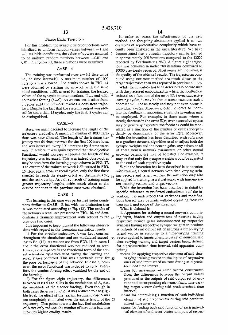
i.e., 65 time intervals). A maximum number of lo00 iterations was allowed. The results shown in FIG. 14 were obtained by starting the network with the same initial conditions, un(0), as used for training, the learned values of the synaptic interconnections, Trim, and with no teacher forcing (A=O). As we can see, it takes about 3 cycles until the network reaches a consistent trajectory. Despite the fact that the system’s output was plotted for more than 15 cycles, only the first. 3 cycles can be distinguished.

CASE-5 Here, we again decided to increase the length of the

trajectory gradually. A maximum number of lo00 iterations was now allowed. The length of the training trajectory was 65 time intervals for the first 100 iterations, and was increased every 100 iterations by 5 time intervals. Therefore, it was again expected that the objective functional would increase whenever the length of the trajectory was increased. This was indeed observed, as may be seen from the learning graph, shown in FIG. 17. The output of the trained network is illustrated in FIG. 15. Here again, from 15 recall cycles, only the first three (needed to reach the steady orbit) are distinguishable, and the rest overlap. As a direct result of training using greater trajectory lengths, orbits much closer to the desired one than in the previous case were obtained.

CASE-6 The learning in this case was performed under condi-

tions similar to CASE-5. but with the distinction that A was modulated according to Eq. (12). The results of the network’s recall are presented in FIG. 16, and dem- onstrate a dramatic improvement with respect to the previous two cases.

It is important to keep in mind the following observations with regard to the foregoing simulation results:

1) For the circular trajectory, A was kept constant throughout the simulations and not modulated according to Eq. (12). As we can see from FIG. 13, in cases 1 and 2 the error functional was not reduced to zero. Hence, a discrepancy in the functional form of the neural activation dynamics used during the learning and recall stages occurred. This was a probable cause for the poor performance of the network. In case 3, however, the error functional was reduced to zero. There- fore, the teacher forcing effect vanished by the end of

5

10

15

20

25

30

35

40

45

14 In order to assess the effectiveness of the new

method, the foregoing simulations applied it to two examples of representative complexity which have recently been analyzed in the open literature. We have demonstrated that a circular trajectory can be learned in approximately 200 iterations compared to the 12000 reported by Pearlmutter (1989). A figure eight trajectory was achieved in under 500 iterations compared to 2oooO previously required. Most important, however, is the quality of the obtained results. The trajectories computed using our new method are much closer to the target trajectories than was reported in previous studies.

While the invention has been described in accordance with the preferred embodiment in which the feedback is reduced as a function of the error E(T) over successive learning cycles, it may be that in some instances such a decrease will not be steady and may not even occur in individual cycles. Moreover, other schemes to modulate the feedback in accordance with the invention may be employed. For example, in those cases where a stead); decrease in the error E(T) over successive cycles may be generally expected, the feedback could be modulated as a function of the number of cycles independently or dependently of the error E(T). Moreover: while the invention has been described with reference to a gradient descent, algorithm used to adjust both the synapse weights and the neuron gains, any subset or all of these neural network parameters or other neural network parameters may be adjusted. For example, it may be that only the synapse weights would be adjusted at the end of each repetitive cycle.

While the invention has been described in connection with training a neural network with time-varying training vectors and target vectors, the invention may also be applied in training neural networks with time-invari- ant training vectors and target vectors.

While the invention has been described in detail by specific reference to preferred embodiments of the invention, it is understood that variations and modifica- tions thereof may be made without departing from the true spirit and scope of the invention.

What is claimed is: 1. Apparatus for training a neural network compris-

ing input, hidden and output sets of neurons having respective neuron gains interconnected by respective synapses having respective synapse weights to produce at outputs of said output set of neurons a time-varying target vector in response to a time-varying training

the learning.

between cases 5 and 6 lies in the modulation of A, @e., the amplitude of the teacher forcing). Even though in both cases the error functional was reduced to a negligi- ble level, the effect of the teacher forcing in case 5 was not completely eliminated over the entire length of the 65 trajectory. This points toward the fact that modulation of A not only reduces the number of iterations but, also provides higher quality results.

2) For the figure eight trajectory, the differences 60

- 50 vector applied to inputs of said input set of neurons, said

time-varying training and target vectors being defmed for a predetermined time interval, said apparatus com-

means for applying respective elements of said time- varying training vector to the inputs of respective ones of said input set of neurons during said predetermined time interval;

prising:

55

means for measuring an error vector constructed from the differences between the output values produced at the outputs of said output set of neurons and corresponding elements of said time-varying target vector during said predetermined time interval,

means for determining a function of each individual element of said error vector during said predetermined time interval;

means for feeding back said function of each individual element of said error vector to inputs of respec-

5,428,7 10 15 16

tive ones of said set of output neurons during said 8. The apparatus of claim 1 further comprising: predetermined time interval; means for progressively decreasing said function in

means responsive to said error vector and to current values of said neuron gains and synapse weights for 9. The apparatus of claim 8 wherein said means for changing at least one of (a) said neuron gains and 5 progressively decreasing said function decreases said (b) said synapse weights in accordance with a gra- function as a function of a decrease in a functional of dient descent algorithm at the end of said predeter- said error vector over said successive ones of said repet- mined time interval to decrease the magnitude of itive cycles. the said error vector; and wherein, 10. The apparatus of claim 9 wherein said functional

said means for applying, said means for measuring, 10 comprises an integral of a function of each element of said means for determining, said means for feeding said error vector measured during a previous one of said back and said means for changing all operate to- repetitive cycles. gether in repetitive cycles, each of said cycles hav- 11. A method for training a neural network comprising a time duration equal to-said predetermined ing input, hidden and output sets of neurons having time interval; and, 15 respective neuron gains interconnected by respective

said means for determining a function of each individ- synapses having respective synapse weights to produce ual element of said error vector comprises means at outputs of said output set of neurons a time-varying for modulating said function in accordance with target vector in response to a time-varying training measurements of said error vector by said means vector applied to inputs of said input set of neurons, said for measuring during a previous one of said repeti- 20 time-varying training and target vectors being defined tive cycles. for a predetermined time interval, said method compris-

inrr:

successive ones of said repetitive cycles.

2. The amaratus of claim 1 wherein said means for I I

modulating said function comprises means for multiplying said function by a factor that depends upon the measurements of all elements of said error vector mea- 25 sured by said means for measuring during an immediately preceding one of said repetitive cycles. 3. The apparatus of claim 2 wherein said factor is 1-

exp, wherein E(7) is an integral over said predetermined time interval of a sum of squares of all elements of the 30 error vector measured during said immediately preceding one of said repetitive cycles. 4. The apparatus of claim 1 wherein said means for

determining a function of each element of said error

5. The apparatus of claim 4 wherein said means for scaling comprise means fox raising each element of said error vector to an exponential power of p , raising the corresponding element of said time-varying target vector to an exponential power of 1-p, and multiplying 40 them together, wherein p is a rational number less than one. 6. The apparatus of claim 5 wherein p is on the order

of approximately 7/9. 7. The apparatus of claim 1 wherein the outputs of 45

each of said neurons obey a set of differential equations during said predetermined time interval, said differential equation being a function of said neuron gains, said synapse weights and said time-varying training and target vectors, and wherein said means for computing 50 said changes by performing a gradient descent algorithm comprise:

means for deriving a set of sensitivity equations from said set of differential equations;

means for solving said set of sensitivity equations 55 once for each one of a set of parameters of said

vector comprises means for scaling said function. 35

I

applying respective elements of said time-varying training vector to the inputs of respective ones of said input set of neurons during said predetermined time interval;

measuring an error vector constructed from the differences between the output values produced at the outputs of said output set of neurons and corresponding elements of said time-varying target vector during said predetermined time interval;

determining a function of each individual element of said error vector during said predetermined time interval;

feeding back said function of each individual element of said error vector to inputs of respective ones of said set of output neurons during said predetermined time interval;

changing at least one of (a) said neuron gains and (b) said synapse weights in response to said error vector and to current values of said neuron gains and synapse weights in accordance with a gradient descent algorithm at the end of said predetermined time interval to decrease the magnitude of the said error vector; and wherein,

said applying, said measuring, said determining, said feeding back and said changing is performed in repetitive cycles, each of said cycles having a time duration equal to said predetermined time interval;

said determining a function of each individual element of said error vector comprises modulating said function in accordance with measurements of said error vector by said measuring during a previous one of said repetitive cycles.

12. The method of claim 11 wherein said modulating

and,

neural network, said parameterscomprising at least one of (a) said neuron gains and (b) said synapse weights;

of each neuron with respect to corresponding ones of said parameters; and

means for computing a change to be made to each one of said parameters at the end of said predetermined time interval by integrating over said prede- 65 preceding one of said repetitive cycles. termined time interval the product of said differential and a corresponding element of said error vector. prises scaling said function.

said function comprises multiplying said function by a factor that depends upon the measurements of all elements of said error vector measured during an immedi-

13. The method of claim 12 wherein said factor is 1-exp wherein E(7) is an integral over said predetermined time interval of a sum of squares of all elements of the error vector measured during said immediately

14. The method of claim 11 wherein said determining a function of each element of said error vector com-

means for computing a differential of the output value 60 ately preceding one of said repetitive cycles.

5428,710 17

15. The method of claim 14 wherein said scaling comprise raising each element of said error vector to an exponential power of p, raising the corresponding element of said time-varying target vector to an exponential power of l-,& and multiplying them together, wherein /3 is a rational number less than one.

16. The method of claim 15 wherein /3 is on the order of approximately 7/9.

17. The method of claim 11 wherein the outputs of each of said neurons obey a set of differential equations during said predetermined time interval, said differential equations depending upon said neuron gains, said synapse weights and said time-varying training and target vectors, and wherein said computing said changes comprises:

deriving a set of sensitivity equations from said set of differential equations;

solving said set of sensitivity equations once for each one of a set of parameters of said neural network, said parameters comprising at least, one of (a) said neuron gains and (b) said synapse weights;

computing a differential of the output value of each neuron with respect to corresponding ones of said parameters; and

computing a change to be made to each one of said parameters at the end of said predetermined time interval by integrating over said predetermined time interval the product of said differential and a corresponding element of said error vector.

18. The method of claim 11 further comprising: progressively decreasing said function in successive

19. The method of claim 18 wherein said progressively decreasing said function comprises decreasing said function in accordance with a decrease in a func-

ones of said repetitive cycles.

18 rons and corresponding elements of said target vector;

means for determining a function of each individual element of said error vector;

means for feeding back said function of each individual element of said error vector to inputs of respective ones of said set of output neurons;

means responsive to said error vector and to current values of said neuron gains and synapse weights for changing at least one of (a) said neuron gains and @) said synapse weights in accordance with a gradient descent algorithm to decrease the magnitude of the said error vector; and wherein,

said means for applying, said means for measuring, said means for determining, said meins for feeding back and said means for changing all operate together in repetitive cycles, each of said cycles having a time duration equal to a predetermined time interval; and,

said means for determining a function of each individual element of said error vector comprises means for modulating said function in accordance with measurements of said error vector by said means for measuring during a previous one of said repeti-

22. The apparatus of claim 21 wherein said means for modulating said function comprises means for multiplying said function by a factor that depends upon the measurements of all elements of said error vector mea-

30 sured by said means for measuring during an immediately preceding one of said repetitive cycles.

23. The apparatus of claim 22 wherein said factor is 1-exp, wherein E(T) is an integral over said predetermined time interval of a sum of squares of all elements

35 of the error vector measured during said immediately

5

10

15

20

25 tive cycles.

tional of said error vector over said successive ones of preceding one of said repetitive cycies. said repetitive cycles. 24. The apparatus of claim 21 wherein said means for

20. A method of training a neural network to output determining a function of each element of said error a target vector in response to a training vector, said vector comprises means for scaling said function. method comprising: 25. The apparatus of claim 24 wherein said means for

feeding back to neuron inputs of said neural network scaling comprise means for raising each element of said a function of an error vector corresponding to a error vector to an exponential power of /3, raising the difference between said target vector and a current corresponding element of said target vector to an expo- output vector of said neural network; and, nential power of l-D, and multiplying them together,

vector while feeding back said function of the error 26. The apparatus of claim 25 wherein p is on the vector; order of approximately 7/9.

modulating said function in accordance with a factor 27. The apparatus of claim 21, wherein the outputs of dependent upon elements of said error vector; each of said neurons obey a set of differential equations

said feeding back is performed in repetitive cycles of 50 during said predetermined time interval, said differen- a cyclic period and cyclically adjusting parameters tial equation being a function of said neuron gains, said of said neural network, and wherein said adjusting synapse weights and said training and target vectors, is performed in accordance with a measurement of and wherein said means for computing said changes by said error vector during a previous one of said performing a gradient descent, algorithm comprise: repetitive cycles. means for deriving a set of sensitivity equations from

21. Apparatus for training a neural network compris- said set of differential equations: ing input, hidden and output sets of neurons having means for solving said set of sensitivity equations respective neuron gains interconnected by respective once for each one of a set of parameters of said synapses having respective synapse weights to produce neural network, said parameters comprising at at outputs of said output set of neurons a target vector 60 least, one of (a) said neuron gains and (b) said syn-

40

stimulating said neural network with said training 45 wherein ,8 is a rational number less than one.

55

in response to a training vector applied to inputs of said input set of neurons, said apparatus comprising:

means for applying respective elements of said training vector to the inputs of respective ones of said input set of neurons; 65

means for measuring an error vector constructed from the differences between the output values produced at the outputs of said output set of neu-

apse weights; means for computing a differential of the output value

of each neuron with respect to corresponding ones of said parameters; and

means for computing a change to be made to each one of said parameters at the end of said predetermined time interval by integrating over said predetermined time interval the product of said differen-

5.428.710 19

tial and a corresponding element of said error vec- t0.r.

28. The apparatus of claim 21 further comprising: means for progressively decreasing said function in

29. The apparatus of claim 28 wherein said means for progressively decreasing said function decreases said function as a function of a decrease in a functional of said error vector over said successive ones of said repetitive cycles.

30. The apparatus of claim 29 wherein said functional comprises an integral of a function of each element of said error vector measured during a previous one of said repetitive cycles.

31. A method for training a neural network comprising input, hidden and output sets of neurons having respective neuron gains interconnected by respective synapses having respective synapse weights to produce at outputs of said output set of neurons a target vector

successive ones of said repetitive cycles.

20 32. The method of claim 31 wherein said modulating

said function comprises multiplying said function by a factor that depends upon the measurements of all elements of said error vector measured during an immedi-

5 ately preceding one of said repetitive cycles. 33. The method of claim 32 wherein said factor is

1-exp, wherein E(T) is an integral over said predetermined time interval of a sum of squares of all elements of the error vector measured during said immediately

34. The method of claim 31 wherein said determining a function of each element of said error vector comprises scaling said function.

35. The method of claim 34 wherein said scaling 15 comprise raising each element of said error vector to an

exponential prover of p, raising the corresponding element of said target vector to an exponential power of 1-p, and multiplying them together, wherein /3 is a rational number less than one.

10 preceding one of said repetitive cycles.

20 36. The method of claim 35 wherein p is on the order of approximately 7/9.

37. The method of claim 31 wherein the outputs of each of said neurons obey a set of differential equations, during said predetermined time interval, said differen-

25 tial equations depending upon said neuron gains, said synapse weights and said training and target vectors, and wherein said computing said changes comprises:

deriving a set, of sensitivity equations from said set, of differential equations;

solving said Set of sensitivity equations Once for each one of a set of parameters of said neural network, said parameters comprising at least one of (a) said neuron gains and (b) said synapse weights;

computing a differential of the output value of each neuron with respect to corresponding ones-of said parameters; and

one of said parameters at the end of said predetermined time interval by integrating over said predetermined time interval the product of said differential and a corresponding element of said error vector.

38. The method of claim 31 further comprising: progressively decreasing said function in successive

39. The method of claim 38 wherein said progressively decreasing said function comprises decreasing said function in accordance with a decrease in a functional of said error vector over said successive ones of said repetitive cycles.

in response to a training vector applied to inputs of said input set of neurons, said method comprising:

applying respective elements of said training vector to the inputs of respective ones of said input set of neurons;

measuring an error vector constructed from the differences between the output values produced at the

and ‘Orre- sponding elements of said target vector;

determining a function of each individual element of 3o said error vector;

feeding back said function of each individual element of said error vector to inputs of respective ones of said set of output neurons;

changing at least One Of (a) said neuron gains and @) 35 said synapse weights in response to said error vector and to current values of said neuron gains and synapse weights in accordance with a gradient descent algorithm to decrease the magnitude of the said error vector; and wherein,

said applying, said measuring, said determining, said feeding back and said changing is performed in repetitive cycles, each of said cycles having a time duration equal to a predetermined time interval; and,

said determining a function of each individual element of said error vector comprises modulating said function in accordance with measurements of said error vector by said measuring during a previous one of said repetitive cycles.

Of said Output set Of

computing a change to be made to

40

ones of said repetitive cycles. 45

* * * * * 50

55

60

65

i 11111 1llllll1111 lllll 11111 11111 11111 ill11 11111 ... 11111 1llllll1111 lllll 11111 11111...

Documents