HYDRAULIC FRACTURE INITIATION IN LIMESTONE

by

Qiao Lu

B.S. Petroleum Engineering, University of Wyoming, 2014

Submitted to the Graduate Faculty of

Swanson School of Engineering in partial fulfillment

of the requirements for the degree of

Master of Science

University of Pittsburgh

2016

ii

UNIVERSITY OF PITTSBURGH

SWANSON SCHOOL OF ENGINEERING

This thesis was presented

by

Qiao Lu

It was defended on

June 10, 2016

and approved by

Andrew P. Bunger, PhD, Assistant Professor, Department of Civil and Environmental Engineering

Eric J. Beckman, PhD, Professor, Department of Chemical and Petroleum Engineering

Robert M. Enick, PhD, Professor, Department of Chemical and Petroleum Engineering

Thesis Adviser: Andrew P. Bunger, PhD, Assistant Professor

iii

Copyright © by Qiao Lu

2016

iv

HYDRAULIC FRACTURE INITIATION IN LIMESTONE

Qiao Lu, M.S.

University of Pittsburgh, 2016

Carbonate-rich rocks such as limestone comprise commonly encountered reservoir rocks in the oil

and gas industry. This thesis is aimed at showing the impact of acidic fluid on hydraulic fracture

initiation through laboratory experimentation. The results show that, compared to water injection,

acid injection results in more rapid initiation of the hydraulic fractures under so-called static fatigue

or pressure-delay conditions wherein a certain pressure, insufficient to instantaneously generate a

hydraulic fracture, is maintained until a hydraulic fracture grows. Acid injection also is shown to

generate a dissolution cavity in the vicinity of the wellbore. The breakdown of the specimen is also

explosive in the case of acid injection, probably due to generate of carbon dioxide as a part of the

dissolution reaction. Finally, the time to breakdown, or specimen lifetime, is shown to be related

not only to the magnitude of the wellbore pressure but also, to the apparent permeability of the

specimen. Taken together, the results indicate firstly that acid injection can be expected to improve

initiation of multiple hydraulic fractures within multistage hydraulic fracturing of horizontal wells

by decreasing the time required for initiation at subcritical wellbore pressures. The results also

show that the current theoretical framework can capture the overall negative exponential

v

relationship between the time to breakdown and the wellbore pressure, but it is insufficient to

account for the secondary dependence on rock permeability.

vi

TABLE OF CONTENTS

TABLE OF CONTENTS ............................................................................................................... vi

LIST OF TABLES ....................................................................................................................... viii

LIST OF FIGURES ....................................................................................................................... ix

ACKNOWLEDGMENTS ............................................................................................................. xi

1.0 INTRODUCTION ......................................................................................................... 1

1.1 OVERVIEW..................................................................................................................... 1

1.2 MOTIVATION ................................................................................................................ 4

1.3 OBJECTIVES ................................................................................................................ 10

2.0 BACKGROUND INFORMATION ............................................................................ 11

2.1 THE CRITERIA OF INSTANTANENOUS BREAKDOWN ...................................... 11

2.2 STATIC FATIGUE ........................................................................................................ 14

2.3 THE INTERRACTION BETWEEN HCL AND CARBONATE ROCK ..................... 15

3.0 EXPERIMENTAL PROCEDURES ............................................................................ 17

3.1 SPECIMEN TYPE ......................................................................................................... 17

3.2 SPECIMEN PREPARATION........................................................................................ 18

3.3 ACID DILUTION .......................................................................................................... 20

3.4 ACID EXPERIMENT FACILITIES ............................................................................. 21

3.4.1 Injection System .......................................................................................... 22

vii

3.4.2 Measurements .............................................................................................. 25

3.5 EXPERIMENTAL PROCEDURES .............................................................................. 26

4.0 RESULT AND DISCUSSION .................................................................................... 28

4.1 WATER EXPERIMENTAL GROUP ........................................................................... 28

4.2 ACID EXPERIMENTAL GROUP ................................................................................ 34

4.3 COMPARISON DISCUSSION ..................................................................................... 40

5.0 CONCLUSIONS .......................................................................................................... 48

REFERENCES ............................................................................................................................. 50

viii

LIST OF TABLES

Table 3-1. Acid use guidelines: carbonate acidizing (from McLeod 1984) ................................. 21

Table 4-1. Water experimental group data ................................................................................... 31

Table 4-2. Acid experimental group data ..................................................................................... 36

ix

LIST OF FIGURES

Figure 1-1. Map of U.S. shale gas and shale oil plays (as of May 9, 2011, from EIA) ................. 3

Figure 1-2. The horizontal well drilled into a shale layer with multiple hydraulic fracture treatment (Modified from KCC 2011) ..................................................................................................... 4

Figure 1-3. Typical decline curve for an unconventional tight and shale gas well (Ali & Sheng 2015) ........................................................................................................................................ 5

Figure 1-4. a) Example of uneven performance of perforation cluster (Cipolla et al. 2011) b) Production log results for gas production normalized by max cluster production rate (Bunger & Cardella 2015) ..................................................................................................................... 6

Figure 1-5. Perforation clusters at horizontal wellbore. A) Initial pressurization, B) After well shut-in (after Bunger and Lu 2015) ......................................................................................... 8

Figure 1-6. Wellbore pressure change during the fracture process ................................................ 9

Figure 2-1. 2-D wellbore stress plane view ................................................................................. 12

Figure 2-2. Wormholes created by acid dissolution of limestone (Fredd and Fogler 1998a) ...... 16

Figure 3-1. Specimen sectional view ........................................................................................... 19

Figure 3-2. Specimen sample ....................................................................................................... 20

Figure 3-3. Plumbing draft for the water acid experiments ......................................................... 22

Figure 3-4. Picture of the acid experimental apparatus ............................................................... 23

Figure 3-5. O-Ring separate pump fluid and HCl ........................................................................ 24

Figure 3-6. Acid reservoir. ........................................................................................................... 25

Figure 4-1. The flow rate and pressure data for water instantaneous breakdown test ................. 29

Figure 4-2. The flow rate and pressure data for water test-1260 psi ........................................... 30

Figure 4-3. The flow rate and pressure data for water test-760 psi ............................................. 30

x

Figure 4-4. Lifetime vs. Pressure for water experiments ............................................................. 31

Figure 4-5. #W3 (2000psi) after breakdown ................................................................................ 32

Figure 4-6. #W6 (1200psi) after breakdown ................................................................................ 33

Figure 4-7. #W13 (660psi) after breakdown ................................................................................ 33

Figure 4-8. The flow rate and pressure data for acid instantaneous breakdown test ................... 35

Figure 4-9. The flow rate and pressure data for acid test-1100 psi .............................................. 35

Figure 4-10. The flow rate and pressure data for acid test- 400 psi ............................................. 36

Figure 4-11. Lifetime vs. Pressure for acid experiments ............................................................. 37

Figure 4-12. #A6 (2050psi) after breakdown ............................................................................... 38

Figure 4-13. #A2 (1000psi) after breakdown ............................................................................... 39

Figure 4-14. The wormhole created at 500 psi (left) and 1100 psi (right) ................................... 39

Figure 4-15. Pressure versus Lifetime for both experimental groups .......................................... 41

Figure 4-16. Pressure versus Flow Rate for both experimental groups ....................................... 42

Figure 4-17. Pressure and Flow Rate versus time for W10 ......................................................... 44

Figure 4-18. Pressure and Flow Rate versus Lifetime for W11 ................................................... 44

Figure 4-19. Lifetime and Flow Rate versus Pressure for water experiments ............................. 45

Figure 4-20. Lifetime and Flow Rate versus Pressure for acid experiments ............................... 46

xi

ACKNOWLEDGMENTS

First of all, I want to thank all the committee members, Dr. Andrew Bunger, Dr. Eric Beckman

and Dr. Robert Enick and other audiences for taking time to participate my MS defense.

Here, I emphasize to thank Dr. Andrew Bunger, my research advisor, who inspires me as an

instructor and trusts me as a friend. I am grateful that he gave me an opportunity to work in his lab

and showed me the way to achieve my goal.

Then I want to thank all my friends and colleagues, as well as the staff from the Department of

Civil Environmental Engineering and the Department of Chemical and Petroleum Engineering.

They gave me endless support. Here, I want to special mention Guanyi, Garrett, scooter and

Hannah. All your efforts are indispensable to my thesis.

Last, I feel grateful to my family and the people who love me. I can’t make it today without

your support and approval.

Special thanks for the support of Schlumberger and the review and discussions from Romain

Prioul, Gallyam Aidagulov, and Elizaveta Gordeliy.

1

1.0 INTRODUCTION

1.1 OVERVIEW

Hydraulic Fracturing has been widely applied in the petroleum industry for over six decades

(Montgomery and Smith 2010). Initially, the hydraulic fracturing treatments were carried out

aiming at eliminating the skin effect around the wellbore in conventional reservoir by increasing

the productivity and injectivity index of production and injection wells respectively (Economides

& Nolte 2000, Chapter 5A). The skin effect is mainly caused by the formation damage during the

drilling process and the residue of mud circulation, which commonly led to a decrease of

permeability. The early treatments demonstrated that by creating hydraulic fractures in the specific

depth and direction, bypassing the near wellbore damaged zone, the skin effect could be greatly

reduced.

In the 1970s and 1980s the attention turned towards use of hydraulic fracturing to enable

economical production of oil and gas from low permeability, so-called “unconventional”

reservoirs, which is defined as the ones that does not meet the criteria for applying conventional

methods. Over the past 15 years this goal has been realized for the vast but challenging resources

associated with source-rock organic-rich shale formations. To illustrate, Figure 1-1 shows that

unconventional reservoir development is expanding all over the United States, providing many

challenges and opportunities for the oil and gas industry (Palisch 2012).

2

Unconventional reservoir features can vary widely meaning different types of treatments can

be applied to optimize the eventual production rate. As one of the most common unconventional

reservoirs, carbonate (e.g. limestone) reservoirs are strongly prone to dissolution in the presence

of hydrochloric acid (HCl). They are also of significant economic importance, not only due to the

famously carbonate-rich reservoirs of the Middle East, but also because several major

unconventional plays in the U.S. which have been branded as “shale” plays, actually entail

stimulation of formations which have very little clay content and very large carbonate content.

These include the major oil-rich Eagle Ford, Bakken, and Niobrara formations (Gamero-Diaz et

al. 2013).

The most common approach to stimulation of horizontal wells is multistage hydraulic fracturing

from horizontal wells, and the least expensive and therefore most popular method is the so-called

plug and perforate method, which is illustrated by Figure 1-2. In this approach, the target

formation is divided into several stages along the horizontal well based on the logging data. For

each stage, there are 3 to 6 clusters, each around 2 feet in length, with 30-100 feet interval between

them. Each cluster is comprised typically of 12-36 perforation holes with about 10 mm diameter

and 100 mm length. These perforation holes, or “tunnels”, are formed by detonating shaped

charges deployed on a so-called “perforating gun”. After the first stage is perforated, the

perforation gun is pulled back to the next stage and fluid is pumped into the first stage through the

tubing. Next, the borehole is cleaned after fracturing, a composite plug is set in order to isolate

prior stage(s), and the perforation gun is used to generate the clusters comprising the next stage.

Stimulation of a 5000-10000 foot long horizontal well typically consists of repetition of this

process 10-30 times (Economides et al. 2012, Chapter 18).

3

Figure 1-1. Map of U.S. shale gas and shale oil plays (as of May 9, 2011, from EIA)

4

Figure 1-2. The horizontal well drilled into a shale layer with multiple hydraulic fracture treatment (Modified from KCC 2011)

1.2 MOTIVATION

Field evidence indicates that treatments are significantly non-optimal, particularly for stimulation

of horizontal wells. A typical decline curve for an unconventional tight and shale gas well is shown

in Figure 1-3. In fact, rapid production decline for horizontal wells in unconventional reservoirs

is widely agreed to be one of their most problematic behaviors. One of the probable root causes of

rapid production decline is non-uniformity of stimulation of the horizontal wells. The result is that

production can be highly non-uniform, presumably leading to rapid depletion of some portions of

5

the reservoir with unproduced hydrocarbons in others. The non-uniformity of production can be

seen in production logs, which are obtained by pulling a spinner-type flow rate measurement

device on a wireline through a producing well. These logs, though run on only a few percent of

wells at most, indicate that 40% of perforation clusters in a typical well produce no hydrocarbons

and, in extreme cases such as the one illustrated in Figure 1-4a, only a few perforation clusters

account for the vast majority of productivity of an entire horizontal well. As a result of these

observations, there is a shared objective in the petroleum industry to improve the uniformity of

stimulation in order to improve overall well performance including reducing the rate of production

decline.

Figure 1-3. Typical decline curve for an unconventional tight and shale gas well (Ali & Sheng 2015)

6

Figure 1-4. a) Example of uneven performance of perforation cluster (Cipolla et al. 2011) b) Production log results for gas production normalized by max cluster production rate (Bunger & Cardella 2015)

The objective of improving the uniformity of stimulation from horizontal wells has motivated

many recent contributions (e.g. Olson and Dahi-Taleghani 2009, Nagel et al. 2011, Peirce and

Bunger 2014). Typically, these focus on mechanisms of multiple fracture growth and interaction.

The initiation of multiple fractures, as the prerequisite condition of multiply fracture growth, is

only beginning to be studied (Bunger & Lu 2015, Lu et al. 2015).

a

b

7

In fact, several classical contributions address the issue of initiation of a single hydraulic

fracture (Hubbert & Wills 1957, Haimson & Fairhurtst 1967). While these theoretical studies can

maybe successfully explain single hydraulic fracture initiation, initiating multiple hydraulic

fractures has its own unique challenges. To see this, consider the hydraulic fracture initiation that

takes place in the adjacent perforation clusters within a single isolated section of wellbore shown

in Figure 1-5 (following Bunger & Lu 2015). Here, Figure 1-5a illustrates four perforation cluster

positions where the hydraulic fractures are intended to initiate during pumping. Here the varying

length of the notch is illustrative of the variability of the reservoir leading to easier fracture

initiation at some clusters compared to others. In this illustration, cluster 3 illustrates the point that

will initiate the hydraulic fracture at the lowest pressure. When pumping commences, the pressure

will increase and firstly approach the initiation pressure at position 3 (Figure 1-6a). Once this

initiation occurs, the pressure is expected to decrease or remain relatively constant, noting that in

applications the pumping rate is controlled, not the pressure. However, based on classical hydraulic

fracture initiation theory, the only way to initiate another hydraulic fracture, i.e. at perforation

cluster number 2, is to increase the pump pressure to reach the new criteria. Because this increase

in pressure while maintaining a constant rate is not expected nor typically observed in pumping

records, one could argue that it is nearly impossible to initiate any additional fractures. If this were

the case, then the expected observation would be that only one perforation cluster would be

stimulated in each stage. However, production logs show that, while results are clearly non-ideal

(e.g. Figure 1-6a), there is ample evidence that multiple hydraulic fracture do often initiate within

a single stage (Figure 1-5b). Therefore, the real situation must be that the hydraulic fracture can

still initiate sometime later with lower pressure than would be required to obtain instantaneous

fracture initiation (e.g. the illustration in Figure 1-6b). We call this delayed hydraulic fracture

8

initiation or pressure-delay initiation phenomenon. The initiation of cluster number 2 seems like

breaking the rules of classical hydraulic fracture initiation theory. The question that comes to us is

this: If the mechanism behind the pressure-delay phenomenon can have a better explanation to the

multiple hydraulic fracture initiation than the classic theory?

The key factor is if this delayed initiation will happen before stopping pumping (Figure 1-6c),

which is a requirement for its practical relevance. Hence, any modifications to the fluid-rock

chemistry that would decrease the time required for delayed initiation at a given pressure are

considered to be advantageous. Indeed, throughout this thesis decreasing the delay time will be

considered synonomous with promoting conditions that are more likely to initiate multiple

hydraulic fractures within a single pumping stage.

Figure 1-5. Perforation clusters at horizontal wellbore. A) Initial pressurization, B) After well shut-in (after Bunger and Lu 2015)

9

Figure 1-6. Wellbore pressure change during the fracture process

Delayed initiation of hydraulic fractures was proposed based on theory by Bunger and Lu (2015).

It has since been verified in the laboratory (Lu et al. 2015, Uwaifo 2015). While these recent

experiments have confirmed the existence of time-dependent hydraulic fracture initiation in

sandstone and granite (Lu et al. 2015). At the same time, there are still some issues to resolve.

Primarily, even lifetime, referring to the time between pressurization and loss of specimen integrity

due to hydraulic fracturing, is dependent on wellbore pressure with an exponential relationship in

general, as predicted by theory, the scatter of the data set indicates that pressure is probably not

the only critical characteristic to the initiation. Secondly, all experiments were conducted under

conditions where no chemical reaction is expected between the rock and fluid. However, it is still

unclear how the pressure-delay phenomenon could also occur in acidic environment. If so, will it

follow the same law like the previous experiments? Besides, many experimental analyses (e.g. Hill

et al. 2007, Wu & Sharma 2015) show that the erosion of acid can weaken the structure strength

10

of rock matrix and make rock easier to break. That idea inspires us to hypothesize that the acidic

fluid injection will reduce the breakdown period and accelerate the speed of delayed initiation. The

use of HCl for this purpose in hydraulic fracturing is proposed for the first time in this thesis and

experimentally evaluating the potential for HCl to reduce the delayed initiation time for hydraulic

fractures is thus motivated.

1.3 OBJECTIVES

In summary of the problems that we mentioned above, the goal of the thesis is to determine:

1) If the pressure-delay phenomenon could also occur in acidic environment in carbonate

rock and compare results with the previous experiments.

2) If acidizing fluid injection can reduce the breakdown period and accelerate the speed of

delayed initiation, thereby bringing the potential to improve horizontal well stimulation in

carbonates by promoting multiple hydraulic fracture initiation during the time period of

the pumping.

3) The critical characteristics to the pressure-delay initiation other than wellbore pressure.

In order to achieve those goals, rock pressure-delay simulation experiments were conducted in lab

scale on limestone by injecting hydrochloric acid (HCl). Before that, water injection pressure-

delay experiments were applied as control group in order to further validate the pressure-delay

breakdown theory and provide a relatively chemically-neutral comparison case for the HCl

experiments.

11

2.0 BACKGROUND INFORMATION

In this chapter, background information that can help to interpret the pressure-delay theory will be

introduced. These include the criteria of instantaneous breakdown, static fatigue theory and the

interaction between hydrochloric acid and carbonate rock. These three sections will successively

explain: 1) the stress distribution near the wellbore, and how these stresses lead to an instantaneous

breakdown, 2) what is the limitation of instantaneous breakdown theory and why static fatigue

theory is a good candidate to make up shortages, and, 3) what are some characteristics of

dissolution of carbonates by HCl that will be relevant to the interpretation of experiments.

2.1 THE CRITERIA OF INSTANTANENOUS BREAKDOWN

Classical theory of hydraulic fracture initiation begins with a 2-D, plane strain analysis of a

pressurized hole in a pre-stressed elastic medium, which is shown in Figure 2-1. Here the

quantities σh, σH, pw, and po are the minimum and maximum components of the horizontal in-situ

stress, wellbore pressure and pore pressure in the reservoir respectively. The in-situ stress here

can be simply understood as the compressive stress applied by the formation far away from the

wellbore. In the 2-D model, a fracture will initiate in the direction of σH and open against σh

direction.

12

Figure 2-1. 2-D wellbore stress plane view

According to the theory which was put forward by Hubbert and Willis (“H-W” 1957) and Haimson

and Fairhurst (“H-F” 1967) and systemized by Detournay and Carbonell (Detournay & Carbonell

1997), the maximum tangential normal stress 𝜎𝜎𝜃𝜃𝜃𝜃𝑚𝑚𝑚𝑚𝑚𝑚 (rock mechanics) is given by

𝜎𝜎𝜃𝜃𝜃𝜃𝑚𝑚𝑚𝑚𝑚𝑚 = β𝑝𝑝𝑤𝑤 − 𝜎𝜎� (3-1)

Where,

𝜎𝜎� = 3𝜎𝜎ℎ − 𝜎𝜎𝐻𝐻 − 2𝜂𝜂𝑝𝑝𝑜𝑜 (3-2)

β = �1, 𝐻𝐻 −𝑊𝑊 (𝑓𝑓𝑓𝑓𝑓𝑓𝑓𝑓)

2(1 − 𝜂𝜂), 𝐻𝐻 − 𝐹𝐹 (𝑓𝑓𝑠𝑠𝑠𝑠𝑠𝑠) (3-3)

Here, the “fast” means the case that pump fluid hardly penetrates the pore spaces and flaws

adjacent to the wellbore and “slow” refers to the case where it does. Also, η is a poreoelastic

constant that is normally in the range from 0 to 0.5, defined by

𝜂𝜂 = 𝑏𝑏(1−2𝜈𝜈)2(1−𝜈𝜈)

where 𝜈𝜈 is the Poisson’s ratio (typically ranging from 0.15 to 0.3 for sedimentary rocks) and b is

the Biot coefficient. The Biot coefficient is typically ranging from 0.6-0.8 for sandstone and

13

limestone (e.g. Detournay & Cheng 2014) and is typically close to 1 for soft, clay-rich shales (e.g.

Sarout and Detournay 2011). The criteria for the rock breakdown, which in these theories is taken

as synonymous with hydraulic fracture initiation, is

𝜎𝜎𝜃𝜃𝜃𝜃𝑚𝑚𝑚𝑚𝑚𝑚 = 𝜎𝜎𝑇𝑇 (3-4)

Where the 𝜎𝜎𝑇𝑇 is the tensile strength of the rock which is a positive number. The wellbore pressure

pw required to achieve this criterion is called the breakdown pressure pb.

If we singly apply the theory above to explain the pressure-delay phenomenon, then the

procedure will be as follows. First, the wellbore pressure will keep increasing to the instantaneous

breakdown pressure corresponding the lowest tangential normal stress. Next the wellbore pressure

will drop after the first hydraulic fracture initiation. Because of the pressure drop, there is no way

to initiate additional fractures since the lower 𝑝𝑝𝑤𝑤 no longer satisfy the criteria. In fact, both plane

strain model developed by Bunger et al. (2010) and radial case by Abbas and Lecampion (2013)

show that the initiation of hydraulic fracture can occur prior to the system reaching the peak

pressure. However, the duration and magnitude of this continued pressure increase after the first

initiation is almost certainly insufficient to explain the relative commonality with which additional

hydraulic fractures appear to initiate within each stage. On the other hand, the successive initiation

of multiple fractures are associating with different time interval, which means the lifetime is also

a characteristic that need to be considered.

In summary, the near wellbore stress concentration mechanism can be valid only in the context

of single hydraulic fracture initiation and hardly explains the pressure-delay mechanism

completely. It is therefore important to pursue a theoretical framework in which hydraulic fractures

can initiate in a delayed manner at pressures below the breakdown pressure. The approach will

14

follow Bunger and Lu (2015), described in Chapter 3, which first requires discussing so-called

static fatigue behavior of rocks.

2.2 STATIC FATIGUE

The phenomenon which materials have been shown to fail after some period of time when they

are exerted by the loading that cannot induce instantaneous failure, is called “static fatigue”. It is

classically defined in the form of a kinetic equation (Zhurkov 1984)

τ = 𝜏𝜏0𝑒𝑒(𝑈𝑈0−𝛾𝛾𝛾𝛾𝑘𝑘𝑘𝑘 ) (3-5)

Here the product of Boltzmann’s constant k and absolute temperature T represents the active level

and the potential kinetic energy stored in all matrix atoms, which makes contribution to break the

interatomic bonds. Thus, the failure stress could be lower by increasing the temperature during a

constant time range. Here U0 is interpreted as the magnitude of the initial energy barrier

determining the probability of breakage of the bonds responsible for strength, which is very close

in magnitude to the binding energy of atoms in material (Zhurkov 1984). By applying the load on

the sample, the energy barrier will decrease linearly with the tensile stress. In our case, it is the

tangential stress which was mentioned in section 3.1. The characteristic time τo was found by

Zhurkov (1984) to be independent of the structure and chemical nature, with magnitude of 10-13

seconds. This is on the order of the period of atomic-scale thermal oscillations. It also represents

the minimum time required to rock failure when 𝑈𝑈0 − 𝛾𝛾𝜎𝜎 =0, also known as instantaneous

breakdown. However, it is quite inconvenient to approach and measure a time period with 10-13

seconds magnitude in reality. In fact, this limit corresponds, according to Zhurkov (1984), to the

limit of dynamic propagation bounded by the wave speed of the material. In our test, we define 1

15

second as instantaneous breakdown time, which is more reasonable and applicable to our cases of

quasi-static crack growth (i.e. with a finite velocity but negligible importance of inertia in the

equations of motion). Here we can see the advantage of static fatigue theory is that it brings time

element into consideration. At the same time, it also indicates the relationship between the lifetime

and stresses, which makes it very likely to be the starting point we are looking for.

2.3 THE INTERRACTION BETWEEN HCL AND CARBONATE ROCK

Hydrochloric acid, as a relatively low price reactant, is usually selected for carbonate acidizing

(Economides & Nolte 2000, Chapter 17). The reaction of interest is a dissolution reaction given

by

𝐶𝐶𝐶𝐶32− + 2𝐻𝐻+ ↔ 𝐻𝐻2𝐶𝐶 + 𝐶𝐶𝐶𝐶2

In practice, injection of HCl into carbonate rocks does not typically generate a steadily moving

dissolution front, but instead creates a so-called wormhole structures. The morphology of the

wormhole structures has been found to relate to a dimensionless number relating the rate of

propagation of the dissolution front to the rate of supply of fluid. This number is known as the

Damkohler number and it is given by

𝐷𝐷𝑓𝑓 = 𝜋𝜋𝜋𝜋𝜋𝜋𝜋𝜋𝑞𝑞

(3-6)

Where d and l are the diameter and length of the flow channel (i.e. pore in the rock matrix)

respectively. Additionally q is the flow rate and κ is the parameter that depend on the dissolution

rate model. More detail can be found in, for example, Fredd and Fogler (1998b).

Experimental examples are shown in Figure 2-2, which we can see the small Damkohler numbers

corresponds to a more complete dissolution at inlet flow face and barely form wormholes. In

16

contrast, intermediate values of Damkohler number corresponds to an obvious wormhole flow

channel, and large Damkohler numbers make the channels more branched. Note, however, that

while it is useful to picture the possibility of wormhole formation and to understand the parameters

controlling wormhole geometry, it is difficult to define Damkohler number in the context of the

present experiments since there are no relevant facilities that can measure the accurate dimensions

of pore-scale flow channels, which are required as inputs to quantify the Damkohler number. That

being said, it remains useful to consider that the higher pressure experiments are expected to result

in higher fluid velocity and therefore smaller Damkohler number than the lower pressure

experiments, meaning that it is possible that different morphologies of the dissolution structure

could occur.

Figure 2-2. Wormholes created by acid dissolution of limestone (Fredd and Fogler 1998a)

17

3.0 EXPERIMENTAL PROCEDURES

This chapter contains the details of the experimental processes used for reaching the research goals.

In addition, the related experimental specimen and facilities information will be introduced. The

process described in detail below includes the following: 1) Preparation of specimens by cutting

to size and drilling the injection hole, 2) Diluting the HCl solution into the desired concentration,

3) Connecting the specimen to the injection system, 4) Performing the experiment, and 5)

Inspecting the specimen and analyzing the data.

3.1 SPECIMEN TYPE

Limestone, which is predominantly composed of calcite and minor amounts of dolomite, is one of

the most common carbonate sedimentary rock that is widely distributed all over the world. It is

also one of the most significant gas and oil-bearing reservoir formations. The current laboratory

experiments use Kasota Valley Limestone, which was quarried from the Minnesota River Valley.

Although it is clearly not a reservoir limestone, it is chosen because it is available with reasonable

uniformity and cost from a commercial quarry (Coldspring quarry, Minnesota).

18

3.2 SPECIMEN PREPARATION

All original rock samples came with saw-cut smooth surfaces and with 6” ×6” ×6” dimensions.

Because our primary work was focusing on the initiation, which took place around the wellbore,

the full size of the specimen was not necessary. Hence the specimens were cut as 3” ×3” ×6” pieces

where the long sides are orthogonal to the bedding layers. By subdividing the 6” cubes more

experiments could be performed and potential errors associated with spuriously varying the

orientation of the wellbore relative to bedding were mitigated.

For consistency with previous experiments in sandstone and granite (Uwaifo 2015, Lu et al.

2015), the injection hole was chosen to be ½” in diameter. It was drilled at the center point of 3”

×3” plane along the 6-inch side, through the entire thickness of the specimen. Next, an 8.5 inch

long by 3/8” outer diameter stainless tubing with 4 perforation holes distributing at symmetrical

positions was put into the wellbore, working as wellbore casing. Based on the American Petroleum

Institute (API) standard grade, the diameter ratio of wellbore to pipe is typically ranging from 1.25

to 1.35; hence the ratio of hole to casing diameter is similar (although it is doubtful this detail is

important). In practice the tube diameter was chosen to allow for a small annulus to accommodate

epoxy that cement the tube in place.

The completion of the analog well is designed to generate a section of pressured wellbore. In

order to do this, two rubber seal O-rings were placed between the wellbore surface and tubing, as

shown in Figure 3-1. These work not only as centralizers but also to isolate the pressurized region.

The tube has holes drilled in it to allow the injected fluid to invade the region between the O-rings

once injection commences. Epoxy adhesive (in this case Sikadur 32) was then placed from both

the top and bottom of the specimen, allowing the adhesive to fill the open collar space from the O-

ring to the surface on both sides. This epoxy holds the tube in place and supports the O-rings

19

holding high pressure. The epoxy adhesive is then allowed at least 12 hours to cure so as to attain

the maximum strength. Finally, a stainless fitting and cap then was fixed on one side of the tubing,

while connecting the other side to the pumping facilities (Figure 3-2). In general, the specimen

would then be placed under triaxial confining stress. However, in this case we wish to make sure

the influence of the wellbore pressure is examined clearly without influence from the confining

pressure, as shown from the H-W and H-F equations. Hence we take here the simplest, cleanest

experiments and explore behavior without confining pressure.

Figure 3-1. Specimen sectional view

20

Figure 3-2. Specimen sample

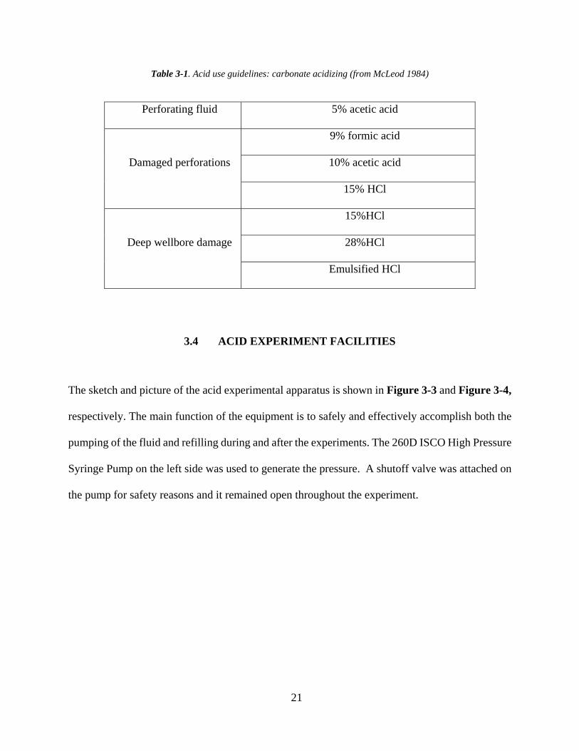
3.3 ACID DILUTION

The hydrochloric acid used in the acid tests is Fisher Chemical Hydrochloric Acid with

manufactural 38% weight percent. Table 3-1 shows suggested acid and concentration for different

treatment purposes. Since we are going to initiate the fracture, 15% weight percent HCl is

recommended. The 15% HCl solution is colorless and transparent liquid, also accompanied with

sharp smell, which is due to the volatility of HCl gas. Thus, to ensure the accuracy of experiments,

the acid needs to be diluted accurately before each test set to minimize the concentration varying

effect. The viscosity of the 15% HCl solution at room temperature is about 1.25~1.31 cp (E.

Nishikata 1981), which will be an important factor that influences the leak off rate during wellbore

pressurization and hydraulic fracture initiation and growth.

21

Table 3-1. Acid use guidelines: carbonate acidizing (from McLeod 1984)

Perforating fluid 5% acetic acid

Damaged perforations

9% formic acid

10% acetic acid

15% HCl

Deep wellbore damage

15%HCl

28%HCl

Emulsified HCl

3.4 ACID EXPERIMENT FACILITIES

The sketch and picture of the acid experimental apparatus is shown in Figure 3-3 and Figure 3-4,

respectively. The main function of the equipment is to safely and effectively accomplish both the

pumping of the fluid and refilling during and after the experiments. The 260D ISCO High Pressure

Syringe Pump on the left side was used to generate the pressure. A shutoff valve was attached on

the pump for safety reasons and it remained open throughout the experiment.

22

3.4.1 Injection System

Figure 3-3. Plumbing draft for the water acid experiments

23

Figure 3-4. Picture of the acid experimental apparatus

In order to prevent the corrosion of the tubing and pump by the HCl, the stainless tubing, indicated

in blue, was replaced by the anti-acid alloy material Monel on the right side, which was marked in

purple (Figure 3-3). Then a mechanical separation was created so that the pump could inject non-

corrosive fluid and the HCl fluid could be delivered to the specimen. To do this, a six-foot-long

by half inch diameter Monel tubing, henceforth referred to as the interface container, was installed

to serve as the acid container during the injection procedure. A PVC plug wrapped by an O-ring

was placed in the tubing to separate the pump fluid and acid (Figure 3-5).

24

Figure 3-5. O-Ring separate pump fluid and HCl

The interface container required refilling immediately before and after each experiment. To

facilitate the filling in a safe and timely manner, another PVC material reservoir (Figure 3-6) was

installed as acid refill tank between interface container and sample. A Monel ball was fixed

underneath to shield the low-pressure reservoir from the high pressures during injection. The

reservoir was wrapped in high-pressure hose sleeve as a secondary containment in case of rupture

from accidental pressurization. As a final safety measure, the sample was enclosed by a 12” ×12”

×12” transparent PVC box, which prevented the acid and rock pieces splashing at breakdown.

25

Figure 3-6. Acid reservoir.

3.4.2 Measurements

The key measurements for these experiments are the fluid pressure and the fluid flow rate. These

were monitored using built-in transducers on the syringe pump. The outputs of these transducers

were connected to a computer via a data acquisition card so the pressure and injection rate could

be recorded throughout the experiment.

26

3.5 EXPERIMENTAL PROCEDURES

An acid pressure-delay initiation test consists of three main steps: 1) acid refill, 2) pressurization,

and 3) clean up. The prepared specimen was connected to the system with all valves closed. These

steps are described in greater detail, below.

Step 1: Acid Refill

At the beginning point, the PVC plug should be at the specimen end of the interface container and

all valves should be shut off. At this time, the interface container will be filled with pump fluid.

The acid refill entails forcing diluted HCl into the interface container, driving the plug back to the

pump end and in doing this, providing an interface container that is filled with dilute HCl and

ready for experimentation.

To begin the refilling, the diluted HCl was poured into the acid reservoir from the top opening.

Then the PVC cap was screwed on the top to isolate the reservoir from air. The next step was to

open the air pump valve, reservoir gate valve and vacuum valve consecutively. The air pressure,

which is regulated down to 40 psi to ensure it will not cause the low-pressure reservoir to rupture,

pushes the HCl back into the interface container until the plug hit the pump-side end. Finally, shut

off all valves and prepared the pressurization process.

Step 2: Pressurization

Prior to commencing pressurization, the first step was to activate the data acquisition card program

which would start to record the pressure and displacement (i.e. volume) reading on the pump.

Subsequently, the pump gate valve and sample gate valve were turned on. Next, the system was

pressurized to 50-100 psi under constant pressure control in order to make sure that all tubing was

27

full filled with HCl and there is no leak-off. Once the pressure reading on the pump was steady,

the goal pressure was applied and held constant until the hydraulic fracture was initiated. Note that

initiation was typically apparent visually as the specimen was observed, and it also was evident

due to a sudden increase in the pumping rate. After the initiation occurred, the pump was stopped

as soon as possible and all valves were turned off again.

Step 3: Clean up

After the experiment was finished, the neutralizer (Na2CO3 solution) was spread by the spray bottle

to neutralize the hydrochloric acid attached on the surface of specimen and PVC box. After that,

the specimen could be removed from the system carefully. Goggles and facemask were worn

throughout the whole experiment for personal protection. All the acid remaining in the interface

container and acid reservoir were then flushed out by opening the pump gate valve and sample

gate valve. Then started the pump with tiny pressure (e.g. 10 psi) to push all the residual acid in

the interface container out. After that, pump gate valve was closed and reservoir gate was turned

on. Pour the water from the top of the reservoir and let it wash through three times to make sure

the reservoir was totally clean.

Note that for the water tests, the process was much easier than the acid tests. The pump was

used directly to inject water into the sample without need for the interfacing apparatus described

above.

28

4.0 RESULT AND DISCUSSION

The data for both experimental groups will be collected and presented respectively in this chapter.

In addition, all observed phenomena during the tests will also be described. The definition of

lifetime and flow rate will be explained in later section. The data for same group will be analyzed

first and then comparison will be made between two different groups. Some unresolved issues will

then be raised and more discussion will be made focusing on that part.

4.1 WATER EXPERIMENTAL GROUP

We have conducted 11 water experiments to study the relationship between lifetime and

breakdown pressure on limestone. Cases that are representative of very fast (“instantaneous”)

breakdown, slow (~600 seconds) breakdown, and intermediate (~100 seconds) breakdown are

portrayed in Figures 4-1 to Figure 4-3. Here, the lifetime of the experiment is defined as the time

to breakdown, i.e. the time between the moment the pressure reaches its nominal constant value

and when the injection rate shoots up with its associated pressure drop. In addition, the flow rate

is recorded when it comes to a steady value, which is essentially the leakoff rate. As we can see,

after the pressurization starts, the flow rate will bump up in order to make pressure reaching the

goal faster.

29

From Figure 4-4, we can see that the pressure-delay phenomenon did occur and the lifetime

showed roughly an exponential relationship with the breakdown pressure. This confirms that

Zhurkov’s theory as adapted for hydraulic fracturing by Bunger and Lu (2015) can provide the

fundamental framework for the pressure-delay phenomenon. Table 4-1 presents the experimental

data. As we can see, the breakdown pressure varies from 2050 psi to 660 psi, corresponding to the

lifetime extending from 1 second to 580 seconds. Here, 2050 psi is found to correspond to the

instantaneous breakdown pressure. However, as mentioned in section 2.2, the strict instantaneous

breakdown takes time in magnitude of 10-13 second, while 1 second is more reasonable for

application to quasi-static fracture growth. A few tests run lower than 650 psi and did not show

any breaks before the pump empty. Thus in our case, 650 psi is considered as the approximate

limit for water pressure delay initiation.

Figure 4-1. The flow rate and pressure data for water instantaneous breakdown test

-50

0

50

100

150

200

250

-500

0

500

1000

1500

2000

2500

0 5 10 15 20 25

Flow

Rat

e (m

l/m

in)

Pres

sure

(psi

)

Time (s)

pump pressure Flow Rate

30

Figure 4-2. The flow rate and pressure data for water test-1260 psi

Figure 4-3. The flow rate and pressure data for water test-760 psi

0

5

10

15

20

25

30

35

40

45

50

-200

0

200

400

600

800

1000

1200

1400

0 20 40 60 80 100 120

Flow

Rat

e (m

l/m

in)

Pres

sure

(psi

)

Time (s)

pump pressure Flow Rate

0

50

100

150

200

250

0

100

200

300

400

500

600

700

800

900

0 50 100 150 200 250 300 350

Flow

Rat

e (m

l/m

in)

Pres

sure

(psi

)

Time (s)

pump pressure Flow Rate

31

Table 4-1. Water experimental group data

Water Test Number

Load Pressure

(psi)

Lifetime (s)

Flow rate (ml/min)

W3 2170 1 185

*W4 1500 5 38

*W6 1340 21 16.5

W19 1260 70 10.5

*W12 1150 20 30

W15 1060 105 12.2

W17 900 200 8

W11 820 840 2.4

W10 810 9 17.5

W20 760 280 6.8

W13 660 580 7.1

Figure 4-4. Lifetime vs. Pressure for water experiments

1

10

100

1000

0 500 1000 1500 2000 2500

Life

time

(s)

Pressure (psi)

32

For each of the water experiments, the fractures propagated approximately parallel to the wellbore,

while the height growth was along the pipe. It is also observed that the dimensions of the fractures

were influenced by the breakdown pressure. Both height and width increased with higher load

pressure (Figure 4-5 to Figure 4-7).

Figure 4-5. #W3 (2000psi) after breakdown

33

Figure 4-6. #W6 (1200psi) after breakdown

Figure 4-7. #W13 (660psi) after breakdown

34

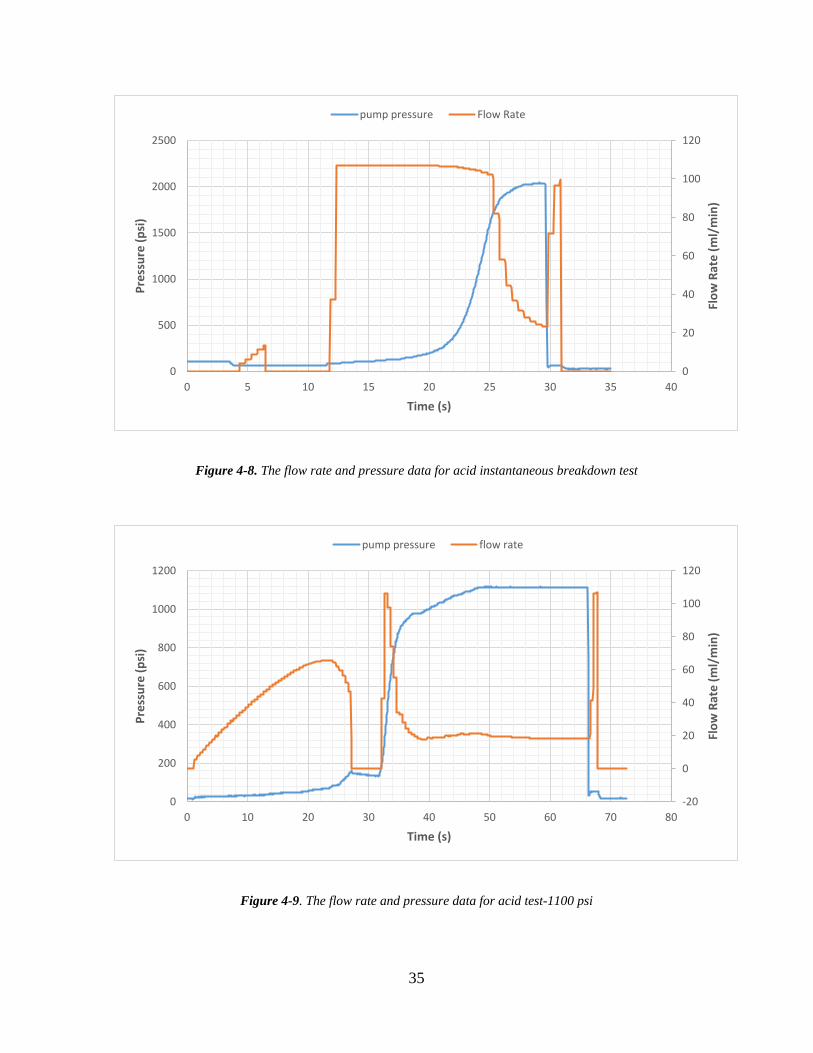
4.2 ACID EXPERIMENTAL GROUP

There were in total 10 acid experiments. These are shown in Table 4-2. Again, representatives of

Figure 4-8 to Figure 4-10, which generally show the same pump pressure curve shape to the water

cases for fast, slow and intermediate lifetimes.

However, there are also some important differences. As we can see from Figure 4-11, in

comparison with the water experimental group, the lifetime of acid group tests shows a tighter

clustering around an exponential relationship with loading pressure. Furthermore, the ability to

attain failure at 400 psi wellbore pressure indicates the reduction of a possible lower limit to the

pressure required for hydraulic fracture initiation. Moreover, the instantaneous breakdown

pressure for the acid is almost the same with the water one. Taken together, it appears that the HCl

does not make a big difference when breakdown is rapid and hence the diffusion of the fluid into

the rock and/or dissolution of the rock does not have time to take place. In this rapid breakdown

limit, the acidic fluid cases appear to work just like normal water. However, at lower pressures and

hence larger times to breakdown, the fluid would appear able to diffuse into the rock and to

generate significant dissolution, which would account for the breakdown occurring at pressures

that did not lead to breakdown with normal water.

35

Figure 4-8. The flow rate and pressure data for acid instantaneous breakdown test

Figure 4-9. The flow rate and pressure data for acid test-1100 psi

0

20

40

60

80

100

120

0

500

1000

1500

2000

2500

0 5 10 15 20 25 30 35 40

Flow

Rat

e (m

l/m

in)

Pres

sure

(psi

)

Time (s)

pump pressure Flow Rate

-20

0

20

40

60

80

100

120

0

200

400

600

800

1000

1200

0 10 20 30 40 50 60 70 80

Flow

Rat

e (m

l/m

in)

Pres

sure

(psi

)

Time (s)

pump pressure flow rate

36

Figure 4-10. The flow rate and pressure data for acid test- 400 psi

Table 4-2. Acid experimental group data

HCl Test

Number

Load Pressure

(psi)

Lifetime (s)

Flow rate (ml/min)

*A6 2040 1 23

*A3 1500 18 9.5

*A10 1350 8 43

*A8 1200 60 7

*A9 1100 22 18.5

A2 1016 100 2.1

A4 800 88 3.6

A5 600 256 4.5

A7 500 314 4

A11 400 1380 1.1

0

2

4

6

8

10

12

14

16

18

20

0

50

100

150

200

250

300

350

400

450

500

0 200 400 600 800 1000 1200 1400 1600

Flow

Rat

e (m

l/m

in)

Pres

sure

(psi

)

Time (s)

pump prerssure Flow Rate

37

Figure 4-11. Lifetime vs. Pressure for acid experiments

Besides the differences in the time to breakdown, or lifetime, in the longer lifetime (lower pressure)

cases, the fracture process observed in the acid experiments appears to be profoundly different

from the water cases. The first striking observation is that the specimens exploded upon breakdown

in the acid cases. In contrast, for the water cases, the breakdown and subsequent fracture growth

led to just a small spurting of fluid when the fracture reached the edge of the specimen. The

resulting blocks were fragmented in the acid cases (Figure 4-12 and Figure 4-13). One possible

explanation for the explosive behavior in the acid cases only is that the dissolution reaction

generates CO2. This produced CO2 would comprise a highly compressible phase, the expansion of

which could be the reason for the explosive behavior.

The second main difference between the acid and water cases is the development of a cavity in

the region of the pressurized section of wellbore in the acid cases. In the water cases there was no

evidence of dissolution. The size of this cavity was typically about several cubic centimeters. There

is evidence that it was created through wormhole formation. This evidence includes pock-marked

1

10

100

1000

10000

0 500 1000 1500 2000 2500

Life

time

(s)

Pressure (psi)

38

morphology and in some cases larger diameter (but still relatively short length) tunnels on the

surface of the fractures. There was also a preponderance of fragmented material after the explosion,

some of which could have been the intact skeleton between the wormholes (Figure 4-14).

Figure 4-12. #A6 (2050psi) after breakdown

39

Figure 4-13. #A2 (1000psi) after breakdown

Figure 4-14. The wormhole created at 500 psi (left) and 1100 psi (right)

40

4.3 COMPARISON DISCUSSION

Since it is still not clear if the acid will reduce the time for initiation, a further group comparison

is made in this section. Figure 4-15 shows us the semi-log plot of lifetime versus pump pressure

for both experimental groups. Under the condition that both trend lines follow an exponential law,

we can see that the acid experiment trend line is shifted down a little bit underneath the water one.

The shift is noticeable at larger times to breakdown, that is, at lower pressures. Note that the

downward shift for lower pressures is understated by the logarithmic scale on the plot. For lifetimes

in the range of 100-1000 seconds, the time to breakdown for the acid cases is 0.1-0.5 times the

time to breakdown for comparable water cases. That is to say, for the same loading wellbore

pressure, the acid treatment can reduce the time to initiation by a factor of 2-10. This reduction

takes place over the practically relevant range as well. In field applications the treatments are

thousands of seconds in duration, so delayed initiation in the order of hundreds of seconds would

occur still relatively early in a hydraulic fracturing treatment.

41

Figure 4-15. Pressure versus Lifetime for both experimental groups

Another observation is that the interception of acid trend line with y-axis is smaller than the water

one. We proposed it indicates a decrease of the energy barrier Uo. This can also explain why the

acid experiments can have a lower pressure criterion to break the rock in a given period of time.

To see this, recall the equation 3-1, which, for zero confining stress (as in these experiments) can

be simplified as

𝜎𝜎𝜃𝜃𝜃𝜃𝑚𝑚𝑚𝑚𝑚𝑚 = β𝑝𝑝𝑤𝑤 (5-1)

Then substitute 5-1 into equation 3-5, leading to

τ = 𝜏𝜏0𝑒𝑒(𝑈𝑈0−𝛾𝛾β𝑝𝑝𝑤𝑤𝑘𝑘𝑘𝑘 ) (5-2)

This shows that 𝑈𝑈𝑜𝑜 − 𝛾𝛾𝛾𝛾𝑝𝑝𝑤𝑤 is proportional to the log of the lifetime τ. If γ and β keep constant,

the decrease of 𝑈𝑈𝑜𝑜will also reduce the requirement of load pressure 𝑝𝑝𝑤𝑤 to approach the specific

lifetime.

The comparison of the flow rates between the acid and water cases also gives rise to some

interesting observations. From Figure 4-16, we can tell that the water experimental group performs

1

10

100

1000

10000

0 500 1000 1500 2000 2500

Life

time

(s)

Pressure (psi)

Water HCl

42

higher flow rate than the acid group in general. On the one hand, this is unexpected under the

premise that dissolution is expected to enhance permeability. However, it is likely that the

decreased flow rate for the acid group is mainly due to the higher viscosity of the acidic fluid. To

see this, consider Darcy’s law

v =𝑘𝑘𝜇𝜇𝛻𝛻 𝑝𝑝

wherein the flow velocity v is proportional to pressure gradient (𝛻𝛻 p) and rock permeability, while

it is inversely proportional to the fluid viscosity if other features keep constant. As mentioned in

section 3.3, the viscosity of 15% HCl solution is about 20-30% higher than the water at room

temperature, which matches the 20-30% lower injection rate for the acidic fluid evidenced in

Figure 4-16.

Figure 4-16. Pressure versus Flow Rate for both experimental groups

05

101520253035404550

400 600 800 1000 1200 1400 1600

Flow

Rat

e (m

l/s)

Pressure (psi)

Water HCl

43

Behind the overall trend, there are still a few unresolved issues. First of all, due to the power

limitation of the pump, it will always take a few second to reach the goal pressure. This period can

be ignored in the long time experiments. However, as for the pressure close to instantaneous

breakdown pressure, the effect of this issue is not negligible anymore. On the one hand, the pump

will pressurize very fast initially in order to reduce injection period. On the order hand, it will slow

down when approaching the goal pressure to avoid over-pumping (e.g. Figure 4-2 and Figure 4-

9). There is another case which the specimen breaks even before reaching the setting pressure (e.g.

Figure 4-8). For both cases, the pressure curve then come out will have smooth slope change which

makes it difficult to define the steady period. Thus, the data whose number is marked with star in

Table 4-1 and Table 4-2 are not completely accurate.

Secondly, W10 and W11, whose data points located far disperse to the trend line, are

questionable. By contrasting the results of water experiments number 10 and 11 (Figure 4-17 and

Figure 4-18), we can see there is a big variation of specimens’ lifetime, even though the load

pressure is pretty much the same. Then we should be aware that, excluding the possible

experimental and human error, there must have some additional phenomena, which led to the huge

difference. The most intuitive variable is the flow rate, which should be proportional to the applied

wellbore pressure. However, the observation indicates that the flow rate of test W10 bumps up

even though the pressure drops, while W11 turned out just the opposite. Therefore, the implicit

assumption of uniformity between samples is not satisfied on these specific samples. That is to

say, the permeability of W10 must be much larger than W11.

44

Figure 4-17. Pressure and Flow Rate versus time for W10

Figure 4-18. Pressure and Flow Rate versus Lifetime for W11

-10

-5

0

5

10

15

20

25

30

35

40

-200

-100

0

100

200

300

400

500

600

700

800

60 65 70 75 80 85 90 95

Flow

Rat

e (m

l/m

in)

Pres

sure

(psi

)

Time (s)

pump pressure Flow Rate

0

1

2

3

4

5

6

7

8

9

10

0

100

200

300

400

500

600

700

800

900

0 200 400 600 800 1000

Flow

Rat

e(m

l/m

in)

Pres

sure

(psi

)

Time (s)

Pump Pressure Flow Rate

45

Based on the phenomenon explained above, we can put forward a hypothesis that besides the load

pressure, the lifetime of the specimen may also depend on the permeability or some other inherent

physical qualities associated with it. Specifically, the higher permeability specimens will lead to a

shorter lifetime at the same pressure when compared to the lower permeability specimens.

Figure 4-19. Lifetime and Flow Rate versus Pressure for water experiments

0

5

10

15

20

25

30

35

40

1

10

100

1000

400 600 800 1000 1200 1400 1600

Flow

Rat

e (m

l/min

)

Life

time

(s)

Pressure (psi)

Lifetime Flow Rate

46

Figure 4-20. Lifetime and Flow Rate versus Pressure for acid experiments

To test this hypothesis, the variation of lifetime and flowrate with respect to pressure are shown in

Figure 4-19 for the water experiments and Figure 4-20 for the acid experiments. Careful

inspection confirms the likely impact of the permeability. The dashed lines in the both figures

illustrate the approximate mean value of lifetime and flow rate at different load pressure, which

means

τ = 𝜏𝜏𝑚𝑚𝑚𝑚𝑚𝑚𝑚𝑚 |𝑝𝑝 𝑖𝑖𝑓𝑓 𝑄𝑄 = 𝑄𝑄𝑚𝑚𝑚𝑚𝑚𝑚𝑚𝑚|𝑝𝑝 (5-3)

Here we can define the flow rate as a linear function of permeability at specific pressure.

Q = 𝛼𝛼𝑘𝑘|𝑃𝑃

Then we can transfer equation 5-3 into

τ = 𝜏𝜏𝑚𝑚𝑚𝑚𝑚𝑚𝑚𝑚 |𝑝𝑝 𝑖𝑖𝑓𝑓 𝑘𝑘 = 𝑘𝑘𝑚𝑚𝑚𝑚𝑚𝑚𝑚𝑚|𝑝𝑝 (5-4)

We can observe the fact that the lifetime τ will be smaller than the 𝜏𝜏𝑚𝑚𝑚𝑚𝑚𝑚𝑚𝑚 if the flow rate k exceeds

then mean value 𝑘𝑘𝑚𝑚𝑚𝑚𝑚𝑚𝑚𝑚 and vice versa.

05101520253035404550

1

10

100

1000

10000

400 600 800 1000 1200 1400 1600 1800 2000

Flow

Rat

e (m

l/min

)

Life

time

(s)

Pressure (psi)

Lifetime Flow Rate

47

All of this is to say, that when the permeability is lower than average, evidenced by the flow

rate plotting below the trendline, then the lifetime is observed to be larger than average, evidenced

by the lifetime plotting above the trendline. The opposite is also true for higher than average

permeability cases – they lead to lower than average lifetime. It is striking that this tendency is

found to hold in all but 2 of the 21 cases presented in the combined water and acid experiments.

The impact of permeability, which is currently not considered in the theoretically-based model,

clearly must be accounted for as a part of future research.

48

5.0 CONCLUSIONS

This thesis describes an experimental research campaign motivated by the potential for the recently

discovered pressure-delay initiation phenomenon in hydraulic fracturing to be impacted by acidic

environments. The mechanism of pressure-delay was investigated experimentally by conducting

rock pressure-delay simulation experiments. In total 21 experiments were performed, 11 with

water and 10 with 15% HCl. Based on the analysis and discussion illustrated above, we can

conclude against the questions proposed in the “Objectives” section:

1. The pressure-delay phenomenon did occur in limestone for both water and acid cases. In

both group experiments, the lifetime of the specimen follows the exponential relationship

with load pressure as a whole, which indicates Zhurkov’s (1984) theory, as adapted for

hydraulic fracture initiation by Bunger and Lu (2015), can basically provide the

fundamental for the pressure-delay phenomenon.

2. The hydrochloric acid treatment can reduce the time needed for the delayed initiation.

when considering the shortening of the initiation period, the performance of acid treatment

is more dramatic for large lifetime (small pressure), since the acid will have more time in

contact with rock matrix.

3. The load pressure is not the only variable that impacts the specimen lifetime. The

permeability or the characteristics that related to it are also likely decisive to the final result.

Besides the conclusions above, some extra conclusions that can be confirmed:

49

4. The instantaneous breakdown pressure for the Kasota Valley Limestone is around 2050 psi,

regardless of the injection fluid. However, the acid experiments have a lower pressure

boundary than the water experiments in the lab scale, which is speculated to be due to the

reduction of the energy barrier. Due to the viscosity increase of the HCl solution, the flow

rate of the acid fluid at steady state is also smaller than the water one.

5. The performance of the hydraulic breakdown in acid experimental group was more violent,

which was in form of severe explosion. The cavity formation was generated on the wellbore

inlet surface, which indicates the successful dissolution of rock matrix.

In the future, based on the conclusions shown above, we can keep investigating the effort of

wormhole structures to the pressure-delayed phenomenon and the method to quantify the

relationship between permeability and lifetime. Besides, in the light of the confining stress applied

in these experiments was zero, more test could be done with varying confining stress to see if the

same results hold under in situ conditions.

50

REFERENCES

Abbas, S., & Lecampion, B. (2013, May 20). Initiation and Breakdown of an Axisymmetric Hydraulic Fracture Transverse to a Horizontal Wellbore. International Society for Rock Mechanics.

Ali, T. A., & Sheng, J. J. (2015, October 13). Production Decline Models: A Comparison Study. Society of Petroleum Engineers. doi:10.2118/177300-MS

Bunger, A. P., & Cardella, D. J. (2015). Spatial distribution of production in a Marcellus Shale well: Evidence for hydraulic fracture stress interaction. Journal of Petroleum Science and Engineering, 133, 162–166. http://doi.org/10.1016/j.petrol.2015.05.021

Bunger, A. P., Lakirouhani, A., & Detournay, E. (2010, August 25). Modelling the Effect of Injection System Compressibility and Viscous Fluid Flow on Hydraulic Fracture Breakdown Pressure. International Society for Rock Mechanics

Bunger, A. P., & Lu, G. (2015, December 1). Time-Dependent Initiation of Multiple Hydraulic Fractures in a Formation with Varying Stresses and Strength. Society of Petroleum Engineers. doi:10.2118/171030-PA

Cipolla, C. L., Weng, X., Onda, H., Nadaraja, T., Ganguly, U., & Malpani, R. (2011, January 1). New Algorithms and Integrated Workflow for Tight Gas and Shale Completions. Society of Petroleum Engineers. doi:10.2118/146872-MS

Detournay, E., & Carbonell, R. (1997). Fracture-mechanics analysis of the breakdown process in Minifracture or Leakoff test. SPE Production & Facilities, 12(03), 195–199. doi:10.2118/28076-pa

Detournay, E., & CHENG, A. H.-D. (2014). Fundamentals of poroelasticity. Analysis and Design Methods: Comprehensive Rock Engineering: Principles, Practice and Projects, II, 113. http://doi.org/10.1016/0148-9062(94)90606-8

Economides, M. J., Hill, D. A., & Ehlig-Economides, C. (2012). Petroleum production systems (2nd ed.). Prentice Hall. Retrieved from http://www.osti.gov/scitech/biblio/274112

51

Economides, M. J., & Nolte, K. G. (2000). Reservoir stimulation. Chichester: J. Wiley.

Fredd, C. N., & Fogler, H. S. (1998, March 1). Alternative Stimulation Fluids and Their Impact on Carbonate Acidizing. Society of Petroleum Engineers. doi:10.2118/31074-PA

Fredd, Christopher N.; Fogler, H. Scott (1998)."Influence of transport and reaction on wormhole formation in porous media." AIChE Journal 44(9): 1933-1949. <http://hdl.handle.net/2027.42/34235>

Gamero-Diaz, H., Miller, C. K., & Lewis, R. (2013, September 30). sCore: A Mineralogy Based Classification Scheme for Organic Mudstones. Society of Petroleum Engineers. doi:10.2118/166284-MS

Haimson, B., & Fairhurst, C. (1967, September 1). Initiation and Extension of Hydraulic Fractures in Rocks. Society of Petroleum Engineers. doi:10.2118/1710-PA

Hill, A. D., Pournik, M., Zou, C., Malagon Nieto, C., Melendez, M. G., Zhu, D., & Weng, X. (2007, January 1). Small-Scale Fracture Conductivity Created by Modern Acid Fracture Fluids. Society of Petroleum Engineers. doi:10.2118/106272-MS

Hoefner, M. L., & Fogler, H. S. (1985). EFFECTIVE MATRIX ACIDIZING IN CARBONATES USING MICROEMULSIONS.Chemical Engineering Progress, 81(5), 40-44.

Hubbert, M. K., & Willis, D. G. (1957, January 1). Mechanics of Hydraulic Fracturing. Society of Petroleum Engineers.

J. Kear, A. P. Bunger, "Dependence of Static Fatigue Tests on Experimental Configuration for a Crystalline Rock", Advanced Materials Research, Vols. 891-892, pp. 863-871, 2014

Lu, G., Uwaifo, E. C., Ames, B. C., Ufondu, A., Bunger, A. P., Prioul, R., & Aidagulov, G. (2015, November 13). Experimental Demonstration of Delayed Initiation of Hydraulic Fractures below Breakdown Pressure in Granite. American Rock Mechanics Association.

McLeod, H. O. (1984, December 1). Matrix Acidizing. Society of Petroleum Engineers. doi:10.2118/13752-PA

Montgomery, C. T., & Smith, M. B. (2010, December 1). Hydraulic Fracturing: History Of An Enduring Technology. Society of Petroleum Engineers. doi:10.2118/1210-0026-JPT

Nagel, N. B., Gil, I., Sanchez-nagel, M., & Damjanac, B. (2011, January 1). Simulating Hydraulic Fracturing in Real Fractured Rocks - Overcoming the Limits of Pseudo3D Models. Society of Petroleum Engineers. doi:10.2118/140480-MS

52

Nishikata, E., Ishii, T., & Ohta, T. (1981). Viscosities of aqueous hydrochloric acid solutions, and densities and viscosities of aqueous hydroiodic acid solutions. Journal of Chemical & Engineering Data, 26(3), 254–256. doi:10.1021/je00025a008

Olson, J. E., & Taleghani, A. D. (2009, January 1). Modeling simultaneous growth of multiple hydraulic fractures and their interaction with natural fractures. Society of Petroleum Engineers. doi:10.2118/119739-MS

Palisch, T. T., Chapman, M. A., & Godwin, J. W. (2012, January 1). Hydraulic Fracture Design Optimization in Unconventional Reservoirs - A Case History. Society of Petroleum Engineers. doi:10.2118/160206-MS

Peirce, A. P., & Bunger, A. P. (2014, August 18). Robustness of Interference Fractures that Promote Simultaneous Growth of Multiple Hydraulic Fractures. American Rock Mechanics Association.

Sarout, J., & Detournay, E. (2011). Chemoporoelastic analysis and experimental validation of the pore pressure transmission test for reactive shales. International Journal of Rock Mechanics and Mining Sciences, 48(5), 759-772.

KCC, (2011). Kansas Corporation Commission, Conservation Division, web page: Kansas Corporation Commission, http://www.kcc.state.ks.us/conservation/index.htm (accessed May 2011)

Uwaifo, E. C. (2015). Time Dependent Initiation of Multiple Hydraulic Facture in Rock. M.S. Thesis. University of Pittsburgh.

Wu, W., & Sharma, M. M. (2015, February 3). Acid Fracturing Shales: Effect of Dilute Acid on Properties and Pore Structure of Shale. Society of Petroleum Engineers. doi:10.2118/173390-MS

Zhurkov, S. N. (1984). Kinetic concept of the strength of solids. International Journal of Fracture,26(4), 295–307. doi:10.1007/bf00962961