how urban planners caused the housing bubble with the deflation of the housing bubble. but what...

Everyone agrees that the recent financial crisisstarted with the deflation of the housing bubble.But what caused the bubble? Answering thisquestion is important both for identifying thebest short-term policies and for fixing the creditcrisis, as well as for developing long-term policiesaimed at preventing another crisis in the future.

Some people blame the Federal Reserve forkeeping interest rates low; some blame theCommunity Reinvestment Act for encouraginglenders to offer loans to marginal homebuyers;others blame Wall Street for failing to properlyassess the risks of subprime mortgages. But all ofthese explanations apply equally nationwide, whilea close look reveals that only some communitiessuffered from housing bubbles.

Between 2000 and the bubble’s peak, infla-tion-adjusted housing prices in California andFlorida more than doubled, and since the peakthey have fallen by 20 to 30 percent. In contrast,housing prices in Georgia and Texas grew byonly about 20 to 25 percent, and they haven’t sig-nificantly declined.

In other words, California and Florida hous-ing bubbled, but Georgia and Texas housing didnot. This is hardly because people don’t want tolive in Georgia and Texas: since 2000, Atlanta,Dallas–Ft. Worth, and Houston have been thenation’s fastest-growing urban areas, each grow-ing by more than 120,000 people per year.

This suggests that local factors, not nationalpolicies, were a necessary condition for the hous-ing bubbles where they took place. The mostimportant factor that distinguishes states likeCalifornia and Florida from states like Georgiaand Texas is the amount of regulation imposed onlandowners and developers, and in particular aregulatory system known as growth management.

In short, restrictive growth management wasa necessary condition for the housing bubble.States that use some form of growth manage-ment should repeal laws that mandate or allowsuch planning, and other states and urban areasshould avoid passing such laws or implementingsuch plans; otherwise, the next housing bubblecould be even more devastating than this one.

How Urban Planners Causedthe Housing Bubble

by Randal O’Toole

_____________________________________________________________________________________________________

Randal O’Toole is a senior fellow with the Cato Institute and author of The Best-Laid Plans: How GovernmentPlanning Harms Your Quality of Life, Your Pocketbook, and Your Future.

Executive Summary

No. 646 October 1, 2009

366545_PA646_1stClass:366545_PA646_1stClass 9/15/2009 12:55 PM

Misconceptions aboutthe Housing Bubble

In 2005, both Alan Greenspan and BenBernanke argued that there was “no housingbubble” and that people need not fear that sucha bubble would burst. Greenspan admittedthere was “froth” in local housing markets butno national bubble. Bernanke argued thatgrowing housing prices “largely reflected strongeconomic fundamentals” such as growth injobs, incomes, and new household formation.1

How could they have gone so wrong?“Bubble deniers point to average prices for thecountry as a whole, which look worrisome butnot totally crazy,” Princeton economist PaulKrugman wrote in a 2005 newspaper column.“When it comes to housing, however, theUnited States is really two countries, Flatlandand the Zoned Zone.” Flatland, he said, hadlittle land-use regulation and no bubble, whilethe Zoned Zone was heavily regulated and was“prone to housing bubbles.”2

Krugman’s choice of terms is unfortunatebecause most of “Flatland” is in fact zoned.What makes the Zoned Zone different is notzoning but growth-management planning, a broadterm that includes such policies as urban-growth boundaries, greenbelts, annual limitson the number of building permits that can beissued, and a variety of other practices.

Growth control, which limits a city’s growth toa specific annual rate, is a form of growth-man-agement planning that was popular in the 1970s.Smart growth, which discourages rural develop-ment and encourages higher-density develop-ment of already developed areas, is another formthat is more popular today. No matter what theform, by interfering with markets for land andhousing, growth-management planning almostinevitably drives up housing prices and is closelyassociated with housing bubbles.

Harvard professor Harvey Mansfield criti-cizes economists for failing to foresee the hous-ing bubble.3 But, in fact, many economists didsee the bubble as it was growing and predictedthat its collapse would lead to severe hardships.

For example, as early as 2003 The Economist

observed, “The stock-market bubble has beenreplaced by a property-price bubble,” and point-ed out that “sooner or later it will burst.”4 By2005, it estimated that housing had become“the biggest bubble in history.” Because of theeffects of the bubble on consumer spending,The Economist warned, the inevitable deflationwould lead to serious problems. “The wholeworld economy is at risk,” the newspaper point-ed out,5 adding, “It is not going to be pretty.”6

Although The Economist did not predict thecomplete collapse of credit markets, it was cor-rect that the bubble’s deflation was not pretty.

After home-price deflation led to the creditcrisis, it became “conventional wisdom thatAlan Greenspan’s Federal Reserve was respon-sible for the housing crisis,” notes HooverInstitution economist David Henderson in acolumn in the Wall Street Journal.7 AlthoughHenderson disagreed with this view, severalother economists writing in the same issueagree that by boosting demand for housing,the Federal Reserve Bank’s low interest ratescaused the housing bubble. “The Fed ownsthis crisis,” charges Judy Shelton, the author ofMoney Meltdown.8

Other people blame the crisis on theCommunity Reinvestment Act and other fed-eral efforts to extend homeownership to low-income families.9 Those policies, along withunscrupulous lenders, fraudulent homebuy-ers, and greedy homebuilders—all of whomhave also been blamed for the housing cri-sis—have two things in common. First, theyfocus on changes in the demand for housing.Second, they are all nationwide phenomena.

National changes in demand should havehad about the same effect on home prices inHouston as in Los Angeles. But they did not.As this paper will show, just as prices rosemuch more dramatically in Krugman’s ZonedZone than in Flatland, prices later fell steeplyin most of the Zoned Zone but—except forstates where home prices declined because ofthe collapse of the auto industry—prices hard-ly fell at all in Flatland. As late as the fourthquarter of 2008, home prices remained stablein many non-bubbling parts of the country.This suggests that the real source of the bub-

2

As late as thefourth quarter of2008, home pricesremained stablein many parts of

the country.


ble was limits on supply that exist in someparts of the country but not in others.

In response to the crisis, some have sug-gested that the federal government shouldbuy surplus homes and tear them down orrent them to low-income families. This mis-reads the crisis, which is not due to a surplusof homes but to an artificial shortage createdby land-use regulation. This shortage pushedup home prices to unsustainable levels, butthat doesn’t mean that there is no demandfor housing at more reasonable prices.

Related to this are increased claims thatthis crisis signals the last hurrah for suburbansingle-family homes. “The American suburbas we know it is dying,” proclaims Timemaga-zine.10 The Atlantic Monthly frets that suburbswill become “the next slums.” Both articlesquote a demographic study that claims that“by 2025 there will be a surplus of 22 millionlarge-lot homes (on one-sixth of an acre ormore) in the U.S.”11 Ironically, articles such asthese promote an intensification of the kindof land-use regulation that created the hous-ing bubbles.

A Theory of theHousing Bubble

Bubbles have characterized recent econom-ic history, as institutional and other majorinvestors have sought high-return, low-riskinvestments. These investments have turnedinto speculative manias that eventually comecrashing down. The last decade alone has seenthe telecom bubble, the nearly simultaneousdot-com bubble, the housing bubble, andmost recently, the oil bubble—all of which ledthe satirical newspaper, The Onion, to report,“Nation Demands New Bubble to Invest In.”12

Of these, the housing bubble is the mostsignificant. On one hand, consumer spendingfed by people borrowing against the temporar-ily increased equity in their homes kept theworld economy going after the high-tech andtelecom bubbles burst in 2001. On the otherhand, the eventual deflation of the housingbubble caused far more severe economic prob-

lems than the deflation of the telecom andhigh-tech bubbles would have caused if thehousing bubble had not disguised them.

A bubble has been defined as “trade in highvolumes at prices that are considerably at vari-ance with intrinsic values.”13 Bubbles are essen-tially irrational, so they are difficult to describewith a rational economic model. However, thepreliminaries to the housing bubble can beexplained using simple supply-and-demandcurves.

Charles Kindleberger’s classic book Manias,Panics, and Crashes describes six stages of a typi-cal bubble. First, a displacementor outside shockto the economy leads to a change in the valueof some good. Second, new credit instrumentsaredeveloped to allow investors to take advantageof that change. This leads to the third stage, aperiod of euphoria, in which investors come tobelieve that prices will never fall. This oftenresults in a period of fraud, the fourth stage, inwhich increasing numbers of people try to takeadvantage of apparently ever-rising prices.Soon, however, prices do fall, and, in the fifthstage, the market crashes. In the sixth and finalstage, government officials try to impose newregulation to prevent such bubbles from tak-ing place in the future.14 All of these stages areapparent in the recent housing bubble. The keypoint of this paper is that because growth con-trols did not allow heightened demand forhousing to dissipate through new supply, theresult was an immense price bubble in stateshousing nearly half of the nation’s population.

Housing markets include both new andused housing. New housing accommodatespopulation growth and replaces both worn-out older housing and housing in areas thatare being converted to other uses. The price ofused housing is set by the cost of new housing.If the price of new housing rises, sellers ofexisting homes will respond by adjusting theirasking prices. Thus, to understand the price ofhousing, we must focus on the supply anddemand curves for new housing.

The steepness of those curves—whicheconomists call elasticity—describes the sensi-tivity of prices to changes in demand or sup-ply. A flat or elastic supply curve, for example,

3

Claims that thesuburbs are dyingare made to support the policies that created the housing bubblesin the first place.


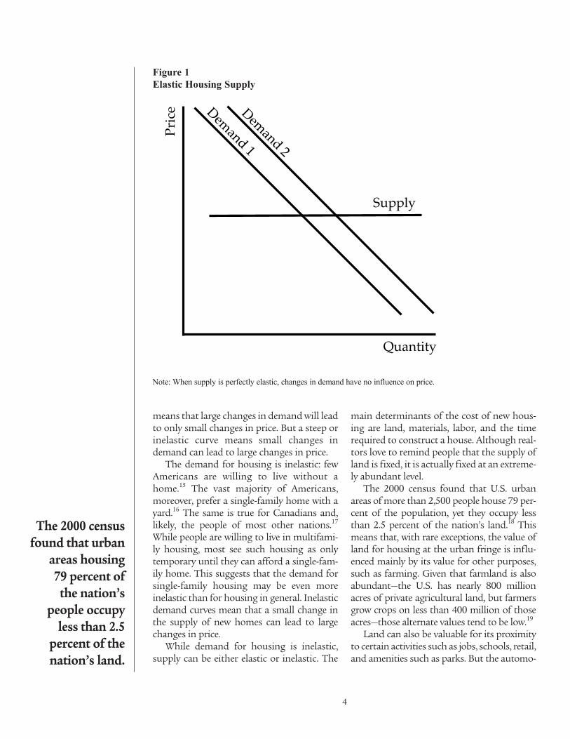
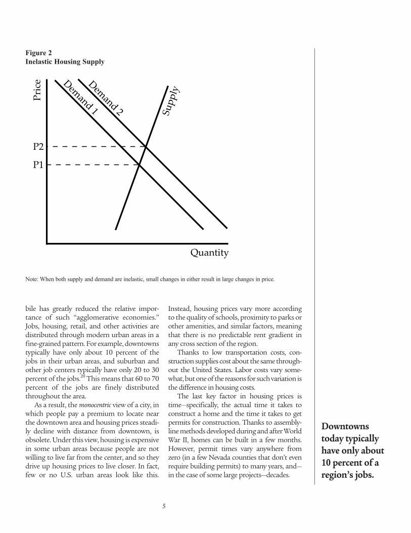
means that large changes in demand will leadto only small changes in price. But a steep orinelastic curve means small changes indemand can lead to large changes in price.

The demand for housing is inelastic: fewAmericans are willing to live without ahome.15 The vast majority of Americans,moreover, prefer a single-family home with ayard.16 The same is true for Canadians and,likely, the people of most other nations.17

While people are willing to live in multifami-ly housing, most see such housing as onlytemporary until they can afford a single-fam-ily home. This suggests that the demand forsingle-family housing may be even moreinelastic than for housing in general. Inelasticdemand curves mean that a small change inthe supply of new homes can lead to largechanges in price.

While demand for housing is inelastic,supply can be either elastic or inelastic. The

main determinants of the cost of new hous-ing are land, materials, labor, and the timerequired to construct a house. Although real-tors love to remind people that the supply ofland is fixed, it is actually fixed at an extreme-ly abundant level.

The 2000 census found that U.S. urbanareas of more than 2,500 people house 79 per-cent of the population, yet they occupy lessthan 2.5 percent of the nation’s land.18 Thismeans that, with rare exceptions, the value ofland for housing at the urban fringe is influ-enced mainly by its value for other purposes,such as farming. Given that farmland is alsoabundant—the U.S. has nearly 800 millionacres of private agricultural land, but farmersgrow crops on less than 400 million of thoseacres—those alternate values tend to be low.19

Land can also be valuable for its proximityto certain activities such as jobs, schools, retail,and amenities such as parks. But the automo-

4

The 2000 censusfound that urbanareas housing 79 percent ofthe nation’s

people occupyless than 2.5 percent of thenation’s land.

Pric

e

Quantity

Demand 1

Demand 2

Supply

Figure 1

Elastic Housing Supply

Note: When supply is perfectly elastic, changes in demand have no influence on price.


bile has greatly reduced the relative impor-tance of such “agglomerative economies.”Jobs, housing, retail, and other activities aredistributed through modern urban areas in afine-grained pattern. For example, downtownstypically have only about 10 percent of thejobs in their urban areas, and suburban andother job centers typically have only 20 to 30percent of the jobs.20 This means that 60 to 70percent of the jobs are finely distributedthroughout the area.

As a result, the monocentric view of a city, inwhich people pay a premium to locate nearthe downtown area and housing prices steadi-ly decline with distance from downtown, isobsolete. Under this view, housing is expensivein some urban areas because people are notwilling to live far from the center, and so theydrive up housing prices to live closer. In fact,few or no U.S. urban areas look like this.

Instead, housing prices vary more accordingto the quality of schools, proximity to parks orother amenities, and similar factors, meaningthat there is no predictable rent gradient inany cross section of the region.

Thanks to low transportation costs, con-struction supplies cost about the same through-out the United States. Labor costs vary some-what, but one of the reasons for such variation isthe difference in housing costs.

The last key factor in housing prices istime—specifically, the actual time it takes toconstruct a home and the time it takes to getpermits for construction. Thanks to assembly-line methods developed during and after WorldWar II, homes can be built in a few months.However, permit times vary anywhere fromzero (in a few Nevada counties that don’t evenrequire building permits) to many years, and—in the case of some large projects—decades.

5

Downtownstoday typicallyhave only about10 percent of aregion’s jobs.

Pric

e

Quantity

Demand 1

Demand 2 Supp

ly

P2

P1

Figure 2

Inelastic Housing Supply

Note: When both supply and demand are inelastic, small changes in either result in large changes in price.


A Normal Housing Market

In a recent attempt to prop up sales, theNational Association of Realtors produced atelevision ad claiming that “on average, homevalues nearly double every 10 years,” which is agrowth rate of about 7 percent per year.21 Thisis true only when areas with restrictive land-use regulations are included in the average.

Prior to 1970, median home prices in thevast majority of the United States were 1.5 to 2.5times median family incomes.22 The mainexception was Hawaii, which, not coincidental-ly, had passed the nation’s first growth-man-agement law in 1961.23 Home-value to incomeratios remain in that range today in most placesthat do not have growth-management plan-ning. In other words, in the absence of govern-ment regulation, median housing prices aver-age about two times median family incomes.

Without supply restrictions, housingprices grow only if median family incomesgrow. Even then, most of the growth in medi-an housing prices is due to people buildinglarger or higher-quality homes, thus increas-ing the value of the median home. The actu-al value of any given home will not growmuch faster than inflation.

In a normal housing market, then, homevalues keep up with inflation and medianhome values keep up with median familyincomes. Markets become abnormal whenthere is some limit on the supply of newhomes—and most such limits result from gov-ernment regulation. The National Associationof Realtors’ claim may be correct when regu-lated housing markets are averaged withunregulated ones, but it is incorrect if it isapplied to unregulated markets alone.

The Extremes:Houston vs. San FranciscoHouston is an example of a place where,

with minimal government regulation, thesupply curve for housing is almost perfectlyelastic. Houston and surrounding areas have

no zoning, so developers face minimal regula-tion when building on vacant land. Oncebuilt, most developers add deed restrictions totheir properties in order to enhance their val-ue for buyers who want assurance that theneighborhood will maintain a positive charac-ter. But these deed restrictions do not impedefurther growth, as there is plenty of land in theregion without such restrictions.24

In the suburbs of Houston, developersoften assemble parcels of 5,000 to 10,000 acres,subdivide them into lots for houses, apart-ments, shops, offices, schools, parks, and otheruses, and then sell the lots to builders. Thedevelopers provide the roads, water, sewer, andother infrastructure using municipal utility dis-tricts, which allow homebuyers to repay theirshare of the costs over 30 years. At any givenmoment, hundreds of thousands of home sitesmight be available, allowing builders to quick-ly respond to changing demand by buildingboth on speculation and for custom buyers.

Between 2000 and 2008, the Houston met-ropolitan area grew by nearly 125,000 peopleper year. This is 10 times faster than popula-tion growth in 85 percent of American metro-politan areas.25 Yet brand-new homes are avail-able in Houston-area developments for lessthan $120,000, and four-bedroom, two-and-a-half bath homes on a quarter-acre lot averageunder $160,000.26 When supply is this elastic,the inelasticity of demand is irrelevant.

In contrast, land-use regulations steepenthe supply curve, making supply as well asdemand inelastic. While the exact nature ofsuch regulations varies from state to state,typically they involve the use of urban-growth boundaries outside of which develop-ment is limited to homes on lots as large as80 acres; a lengthy and uncertain permittingprocess; high impact fees; and frequent pas-sage of new regulations that make subdivi-sion and construction increasingly costly anddifficult.

The eight counties in the San Francisco BayArea, for example, have collectively drawnurban-growth boundaries that exclude 63 per-cent of the region from development. Regionaland local park districts have purchased more

6

Houston’s minimal

government regulation allowshomebuilders to provide for125,000 new

residents a yearwhile keeping theprice of a 2,200-

square-foot homewell under$200,000.


than half of the land inside the boundaries foropen space purposes. Virtually all of theremaining 17 percent has been urbanized,making it nearly impossible for developers toassemble more than a few small parcels of landfor new housing or other purposes.27

Urban-growth boundaries and greenbeltsnot only drive up the cost of new homes, theymake each additional new housing unit moreexpensive than the last. In other words, theysteepen the supply curve.

Once growth boundaries are in place, citiesno longer need to fear that developers will sim-ply build somewhere else. This gives the citiescarte blanche to pass increasingly restrictiverules on new construction. In places likeHouston, such rules would drive developers tounregulated land in the suburbs. In the SanFrancisco Bay Area, the nearest relatively (withemphasis on “relatively”) unregulated land isin the Central Valley, 60 to 80 miles away.

An onerous permitting process can signif-icantly delay developments both large andsmall. Scott Adams, the creator of the Dilbertcomic strip, reports that it took him morethan four years to gain approval to build onehome in the San Francisco Bay Area.28

Approval of larger developments can takeeven longer and is highly uncertain. When SanJose drew its urban-growth boundary in 1974,it set aside a 7,000-acre area known as CoyoteValley as an “urban reserve” that supposedlywould be brought into the boundary whenneeded. Nearly 30 years later, after inflation-adjusted housing prices had more thanquadrupled, the city finally offered developersan opportunity to propose a plan for buildingin Coyote Valley. After spending $17 millionand five years on planning, however, develop-ers announced in 2008 that they were givingup because there was “simply too much uncer-tainty surrounding the plan and the market tocontinue as is.” Developers doubted the citywould have approved the plan, and even ifapproval were given, environmental groupswere likely to delay development even furtherthrough legal challenges.29

A lengthy permitting process makes itimpossible for developers and homebuilders

to quickly respond to changes in demand.California developers responding to theincrease in housing demand in 2000 wereunlikely to have increased the amount ofproduct they would have brought to marketbefore the prices collapsed in 2006. Emptyhomes in states with growth-managementplanning are symptoms of planning delays,not of any actual housing surplus.

Legal challenges can add to both delays anduncertainties in home construction. Growth-management planners believe almost anyoneshould have the right to challenge developmentof private land on the grounds that property isreally a “collective institution,” says Eric Frey-fogle in his book, The Land We Share. “Whenproperty rights trump conservation laws, theycurtail the positive liberties of the majority.”30

In other words, if the majority of people decidethat your land should be preserved as their“scenic viewshed,” you can effectively lose theright to use it yourself.

In Oregon, for example, the courts grantstanding to anyone trying to stop a develop-ment as long as they say they have someinterest, however slight, in the property. Inone case, a challenger was granted standingbecause she “pass[ed] by the property regu-larly” (it was on a major highway) and usednearby areas “for passive recreation, includ-ing the viewing of wildfowl.”31

These challenges have a major effect on thetype of housing built in a region. Homeownersare more likely to object to new homes thatcost less than their own homes, which are per-ceived as “bringing down the neighborhood.”They also tend to oppose higher-density devel-opments because of the potential effects ontraffic and other issues. At lower densities,homes must cost more to cover the costs ofland and permitting.

For example, a developer once proposed tobuild 2,200 homes on 685 acres in Oakland,California. After eight years, the developerfinally received a permit to build 150 homes,each of which ended up selling for six times asmuch as the homes in the original plans.32

Regions that use growth management arealso more likely to charge stiff developer fees to

7

Oregon courtsgrant standing to anyone whowants to challenge a proposed development,even if their onlyinterest in theproperty is forbirdwatching.


cover infrastructure costs. Whereas Houstondevelopers allow homebuyers to pay off infra-structure costs over 30 years, impact fees ordevelopment charges require up-front pay-ments often totaling tens of thousands of dol-lars. The difference is crucial for housingaffordability: since development charges in-crease the cost of new housing, sellers of exist-ing homes can get a windfall by raising theprice of their houses by an amount equal tothose charges, thus reducing the general levelof housing affordability.

Increasing land and housing costs makeother things more expensive as well. Whenhousing is more expensive, for example, busi-nesses must pay their employees more so thatworkers can afford to live in the region.

A 2002 study broke down the difference inthe costs of a new home in San Jose, which hashad an urban-growth boundary since 1974,and Dallas, which has zoning but whose sub-urbs remain, like Houston’s, almost complete-ly unregulated. Some of the key findings wereas follows:

• The biggest difference was in land costs:A 7,000-square-foot lot in Dallas costonly $29,000, while a 2,400-square-footlot in San Jose cost $232,000.• San Jose’s lengthy permitting process(and the high risk that a permit will neverbe issued) added $100,000 to the cost of ahome in San Jose, while permitting costless than $10,000 per home in Dallas.• To help pay for roads, schools, and oth-

er services, San Jose charged impact feesof $29,000 per new residence, whereasDallas charged only $5,000.•Due mainly to high housing prices forworkers, San Jose construction laborcosts are higher: $143,000 for a three-bed-room house compared with $100,000 inDallas.33

When planners make housing unafford-able, their first response is to impose “afford-ability mandates” on builders. Typically, suchregulations require builders to sell 15 to 20percent of their homes below cost to low-

income buyers. Far from making housingmore affordable, such mandates make it lessaffordable as builders build fewer homes andpass the costs on to the buyers of the other 80to 85 percent of homes. This in turn raises thegeneral price of housing in the region. Oneeconometric analysis found that such afford-ability mandates increased housing prices by20 percent.34

Land-use regulation can affect prices inother ways as well. A wide range of home-builders compete for business in relativelyunregulated markets, ranging from smallcompanies that produce only a few homeseach year, to medium-sized companies thatproduce a few hundred homes per year, togiant national companies that build thou-sands of homes in many different states.Excessive regulation tends to put the smallcompanies out of business and discourage thenational companies as well. The resulting lossof competition helps keep home prices high.Portland, Oregon’s, “urban-growth boundaryhas really been our friend,” says one mid-sizedPortland homebuilder. “It has kept the majorbuilders out of the market.”35

Given that both demand and supply inregulated regions are inelastic, small changesin either one can result in large changes inprice. If lower interest rates increase demandfor housing, Houston-area homebuildersrespond by building more homes; SanFrancisco-area builders respond by filingmore applications, which may wait severalyears for approval. If government purchase ofa large block of land for a park or open spacerestricts supply, Houston-area builders cansimply go somewhere else nearby; in the SanFrancisco area, the nearest alternative build-ing location is more than 50 miles away.

Notice that inelastic supply not onlymakes housing prices rapidly increase withsmall increases in demand; it also makeshousing prices rapidly fall with smalldecreases in demand. This is exacerbated bylengthy permitting periods that can puthomebuilders out of phase with the market.Thus, land-use restrictions create conditionsripe for housing bubbles.

8

When plannersmake housingunaffordable,

their firstresponse is to

require developers to sell

some of theirhomes to low-

income families.


Supply and demand charts only go so farin explaining bubbles. The recent bubble wasprobably exacerbated as much by money flee-ing the post–dot-com bubble stock marketthan by loose credit. Investors looking forsafe places to put their money quickly notedthat housing prices were increasing at dou-ble-digit rates in California, Florida, and oth-er places with growth management policies.At this point, home sales were driven by spec-ulation as much as by the need for shelter.

For example, because of the dot-com crash,San Jose lost 17 percent of its jobs between2001 and 2004. In the same period, officevacancy rates increased from 3 to 30 percent.36

Yet, between the beginning of 2001 and theend of 2004, home prices increased by morethan 20 percent.

This rise in prices in the face of decliningdemand can be attributed to speculation—that is, people buying homes as sources ofincome rather than for shelter. Even thosewho are buying for shelter will pay more for ahouse than its fundamental value (as mea-sured by rents) if they believe, as the NationalAssociation of Realtors claims, that it is a safeinvestment. So the sharp rises in price causedby growth management turn into sharper ris-es caused by people seeing housing as aninvestment.

Houston and the San Francisco Bay Areaare at the extremes of a continuum betweenalmost no regulation and highly intrusiveland-use regulation. Within that continuum,there appear to be five ways in which growthmanagement can influence housing prices:

First, as of 2000, when housing prices werebeginning to bubble, 12 states had passedgrowth-management or smart-growth laws,including Arizona, California, Connecticut,Florida, Hawaii, Maryland, New Jersey, Oregon,Rhode Island, Tennessee, Vermont, and Wash-ington.37 Those laws generally require allmunicipalities to write and follow growth-man-agement plans. In a few cases, the plans are writ-ten by the state itself.

Second, most New England states havelargely abandoned the county level of govern-ment. This effectively gives cities growth-

management authority over the countrysidearound them.

Third, Nevada is a unique case where near-ly all of the land in the state is owned by thefederal government. The rapid growth of LasVegas and Reno have been enabled by federalland sales, but concerns over environmentalissues slowed such sales after 2000 and led torising prices. Moreover, under the SouthernNevada Public Land Management Act of1998, most of the revenue from land sales inClark County (Las Vegas) is dedicated to buy-ing open space and other amenities.38 Sincethen, nearly half the revenues from land saleshave been used to buy parklands, effectivelyrequiring developers to buy two acres from thefederal government to net one more acre ofdevelopable land.39 In effect, Nevada growthmanagement is regulated at the federal level.

Fourth, some counties or urban areas im-plemented growth-management plans with-out state mandates. Prominent examples in-clude Denver-Boulder; Minneapolis–St. Paul;Missoula, Montana; and Charleston, SouthCarolina. This can produce local bubbles thatare sometimes obscured when examiningdata at the state level.

Fifth, and finally, some major urban areasmay not have coordinated growth-manage-ment plans, yet they are hemmed in by state orlocal areas that do have such plans. Washing-ton, DC, has no growth-management plan, butMaryland has a statewide growth-manage-ment law and selected counties in northernVirginia have also begun to practice growthmanagement. New York has no state growth-management law, and prices in upstate NewYork did not bubble. But New York City pricesbubbled, partly because it is hemmed in byConnecticut and New Jersey. Table 1 showswhich form of growth management, if any,affects housing in each state.

State Housing Bubbles

A careful examination of home price datafor the 50 states and 384 metropolitan areasreveals strong correlations between growth-

9

A 1998 federallaw dedicates half the revenuesfrom federal landsales in southernNevada to landpreservation, sodevelopers haveto buy two acresto net one developable acre.


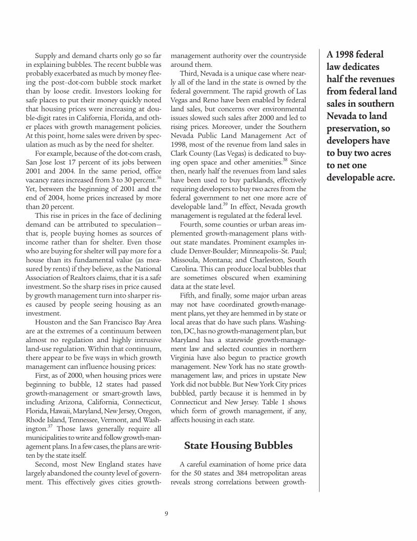
management planning and housing bubbles.The home price indices used in this and otherfigures are published by the Federal HousingFinance Agency (formerly the Office of FederalHousing Enterprise Oversight) and are basedon the Case-Schiller method of comparingchanges in prices of same-home sales overtime.40

On a state level, the biggest housing bubbleswere in six states. Five of the states—Arizona,California, Florida, Maryland, and RhodeIsland—have growth-management laws, whilethe sixth state, Nevada (Figure 3), does not.41 Inall of these states, inflation-adjusted prices roseby 80 to 125 percent after 2000 and dropped by10 to 30 percent after their peak.42 Even thoughseveral of these states are located at oppositecorners of the country, the price indices are verysimilar.

Prices in all but one of the other states withgrowth-management laws, including the NewEngland states, also increased by 50 to 100percent after 2000 and have declined since

2006, in most cases by 5 to 15 percent. Theexception is Tennessee, whose price trends arenearly identical to those in Georgia and Texas(Figure 4). Tennessee housing did not bubblebecause its law was passed in 1998 and theurban-growth boundaries drawn by the citieswere so large that they did not immediatelyconstrain homebuilders.

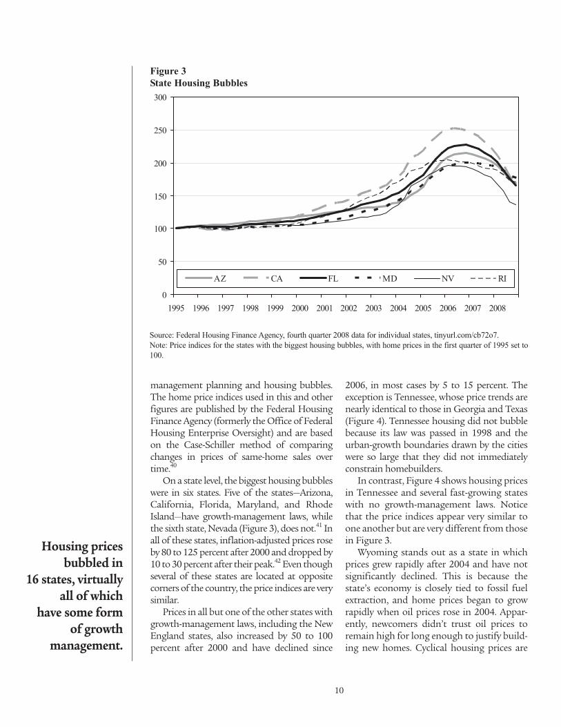
In contrast, Figure 4 shows housing pricesin Tennessee and several fast-growing stateswith no growth-management laws. Noticethat the price indices appear very similar toone another but are very different from thosein Figure 3.

Wyoming stands out as a state in whichprices grew rapidly after 2004 and have notsignificantly declined. This is because thestate’s economy is closely tied to fossil fuelextraction, and home prices began to growrapidly when oil prices rose in 2004. Appar-ently, newcomers didn’t trust oil prices toremain high for long enough to justify build-ing new homes. Cyclical housing prices are

10

Housing pricesbubbled in

16 states, virtuallyall of which

have some form of growth

management.

0

50

100

150

200

250

300

1995 1996 1997 1998 1999 2000 2001 2002 2003 2004 2005 2006 2007 2008

AZ CA FL MD NV RI

Figure 3

State Housing Bubbles

Source: Federal Housing Finance Agency, fourth quarter 2008 data for individual states, tinyurl.com/cb72o7.

Note: Price indices for the states with the biggest housing bubbles, with home prices in the first quarter of 1995 set to

100.


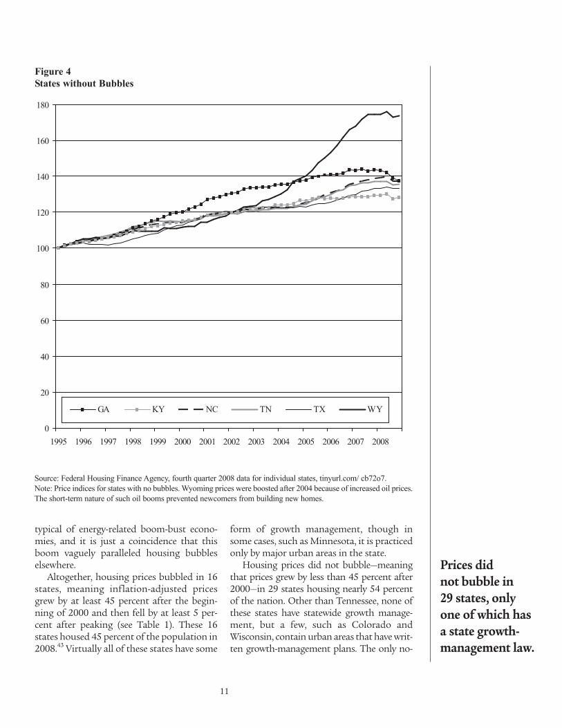
typical of energy-related boom-bust econo-mies, and it is just a coincidence that thisboom vaguely paralleled housing bubbleselsewhere.

Altogether, housing prices bubbled in 16states, meaning inflation-adjusted pricesgrew by at least 45 percent after the begin-ning of 2000 and then fell by at least 5 per-cent after peaking (see Table 1). These 16states housed 45 percent of the population in2008.43 Virtually all of these states have some

form of growth management, though insome cases, such as Minnesota, it is practicedonly by major urban areas in the state.

Housing prices did not bubble—meaningthat prices grew by less than 45 percent after2000—in 29 states housing nearly 54 percentof the nation. Other than Tennessee, none ofthese states have statewide growth manage-ment, but a few, such as Colorado andWisconsin, contain urban areas that have writ-ten growth-management plans. The only no-

11

Prices did not bubble in 29 states, onlyone of which hasa state growth-management law.

0

20

40

60

80

100

120

140

160

180

1995 1996 1997 1998 1999 2000 2001 2002 2003 2004 2005 2006 2007 2008

GA KY NC TN TX WY

Figure 4

States without Bubbles

Source: Federal Housing Finance Agency, fourth quarter 2008 data for individual states, tinyurl.com/ cb72o7.

Note: Price indices for states with no bubbles. Wyoming prices were boosted after 2004 because of increased oil prices.

The short-term nature of such oil booms prevented newcomers from building new homes.


12

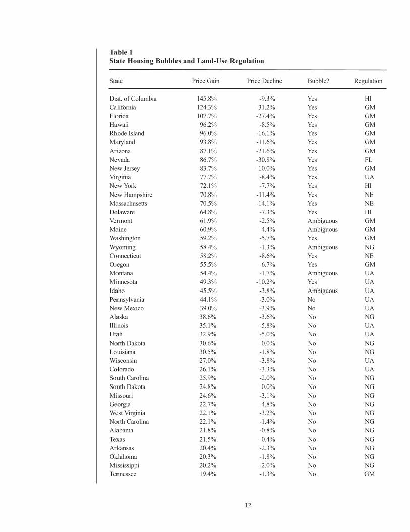
Table 1

State Housing Bubbles and Land-Use Regulation

State Price Gain Price Decline Bubble? Regulation

Dist. of Columbia 145.8% -9.3% Yes HI

California 124.3% -31.2% Yes GM

Florida 107.7% -27.4% Yes GM

Hawaii 96.2% -8.5% Yes GM

Rhode Island 96.0% -16.1% Yes GM

Maryland 93.8% -11.6% Yes GM

Arizona 87.1% -21.6% Yes GM

Nevada 86.7% -30.8% Yes FL

New Jersey 83.7% -10.0% Yes GM

Virginia 77.7% -8.4% Yes UA

New York 72.1% -7.7% Yes HI

New Hampshire 70.8% -11.4% Yes NE

Massachusetts 70.5% -14.1% Yes NE

Delaware 64.8% -7.3% Yes HI

Vermont 61.9% -2.5% Ambiguous GM

Maine 60.9% -4.4% Ambiguous GM

Washington 59.2% -5.7% Yes GM

Wyoming 58.4% -1.3% Ambiguous NG

Connecticut 58.2% -8.6% Yes NE

Oregon 55.5% -6.7% Yes GM

Montana 54.4% -1.7% Ambiguous UA

Minnesota 49.3% -10.2% Yes UA

Idaho 45.5% -3.8% Ambiguous UA

Pennsylvania 44.1% -3.0% No UA

New Mexico 39.0% -3.9% No UA

Alaska 38.6% -3.6% No NG

Illinois 35.1% -5.8% No UA

Utah 32.9% -5.0% No UA

North Dakota 30.6% 0.0% No NG

Louisiana 30.5% -1.8% No NG

Wisconsin 27.0% -3.8% No UA

Colorado 26.1% -3.3% No UA

South Carolina 25.9% -2.0% No NG

South Dakota 24.8% 0.0% No NG

Missouri 24.6% -3.1% No NG

Georgia 22.7% -4.8% No NG

West Virginia 22.1% -3.2% No NG

North Carolina 22.1% -1.4% No NG

Alabama 21.8% -0.8% No NG

Texas 21.5% -0.4% No NG

Arkansas 20.4% -2.3% No NG

Oklahoma 20.3% -1.8% No NG

Mississippi 20.2% -2.0% No NG

Tennessee 19.4% -1.3% No GM


bubble states with significant price declinesare Michigan and Ohio, and those declines aredue to contractions in manufacturing, not ahousing bubble.

The remaining five states, whose prices roseby more than 45 percent but shrank by lessthan 5 percent, are ambiguous. These stateshouse less than 2 percent of the population andinclude one with a growth-management law(Vermont), one with no growth management(Wyoming), and three with controls in a fewurban areas (Idaho, Maine, and Montana).44

There is a strong correlation between fore-closure rates and growth-management-in-duced housing bubbles. As of January 2009,one out of every 173 homes in California wasin foreclosure. The rate in Arizona was 1 in182; Florida was 1 in 214; Nevada was 1 in 76;and Oregon was 1 in 357—all of which areworse than Michigan (1 in 400), despite thelatter having the nation’s highest unemploy-ment rate. By comparison, barely 1 in 1,000Texas homes was in foreclosure. The rate inGeorgia was 1 in 400, North Carolina was 1 in1,700, and Kentucky was 1 in 2,800. The cor-relation is not perfect, but the hardest-hitstates all have some form of growth-manage-ment planning.45

Metropolitan AreaHousing Bubbles

Figure 5 shows home price trends in theSan Francisco Bay area and the Merced,Modesto, and Stockton metropolitan areasin central California. The latter areas enjoyedsome of the biggest price increases after 2000and suffered the largest price declines sincethe top of the housing bubble.46

In 1963, the California legislature passed alaw effectively (though unintentionally) autho-rizing cities and counties to do growth-man-agement planning.47 The counties in the SanFrancisco Bay Area used this law to imposeurban-growth boundaries in the mid 1970s.This made Bay Area housing some of the mostexpensive in the nation, and by the 1990s,increasing numbers of Bay Area workers werebuying homes in relatively affordable centralCalifornia, some 50 to 80 miles away.

Central California counties were lessprone to adopt strict growth-managementplans. But in 2000, the California legislatureamended the law to mandate growth-man-agement planning by all cities and counties.This new mandate, combined with the over-flow from the Bay Area, caused central

13

There is a strongcorrelationbetween foreclosure ratesand growth-management-induced housingbubbles.

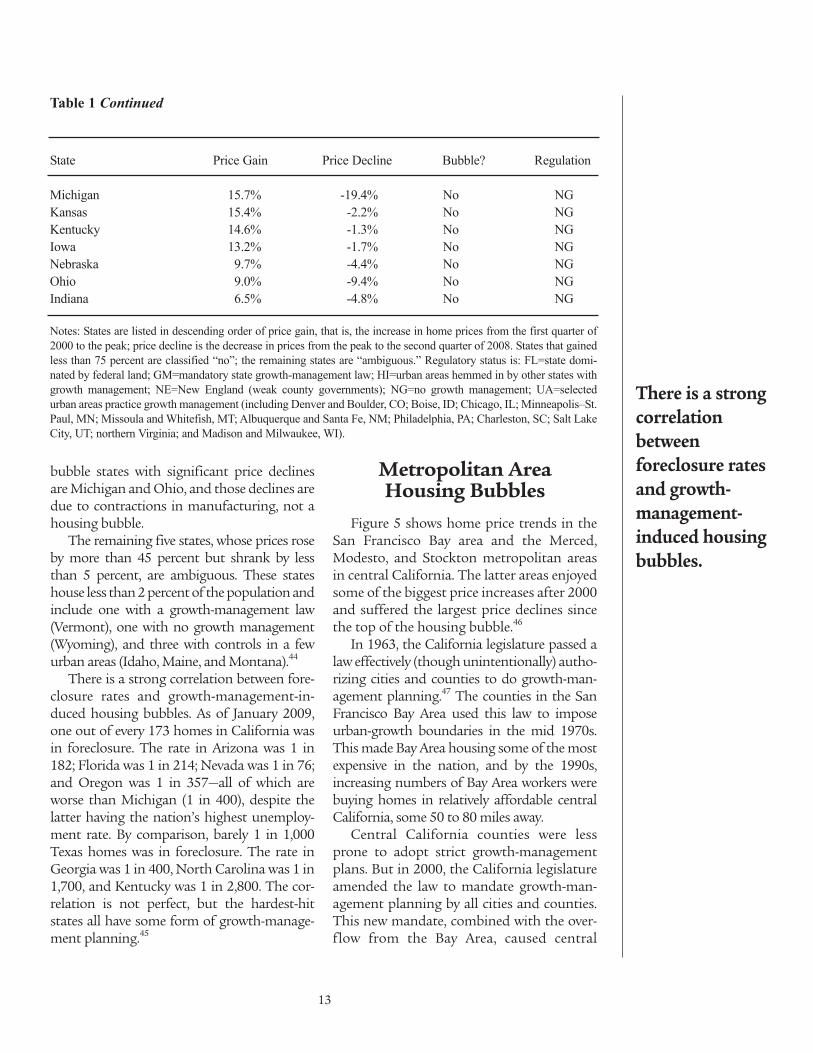
Table 1 Continued

State Price Gain Price Decline Bubble? Regulation

Michigan 15.7% -19.4% No NG

Kansas 15.4% -2.2% No NG

Kentucky 14.6% -1.3% No NG

Iowa 13.2% -1.7% No NG

Nebraska 9.7% -4.4% No NG

Ohio 9.0% -9.4% No NG

Indiana 6.5% -4.8% No NG

Notes: States are listed in descending order of price gain, that is, the increase in home prices from the first quarter of

2000 to the peak; price decline is the decrease in prices from the peak to the second quarter of 2008. States that gained

less than 75 percent are classified “no”; the remaining states are “ambiguous.” Regulatory status is: FL=state domi-

nated by federal land; GM=mandatory state growth-management law; HI=urban areas hemmed in by other states with

growth management; NE=New England (weak county governments); NG=no growth management; UA=selected

urban areas practice growth management (including Denver and Boulder, CO; Boise, ID; Chicago, IL; Minneapolis–St.

Paul, MN; Missoula and Whitefish, MT; Albuquerque and Santa Fe, NM; Philadelphia, PA; Charleston, SC; Salt Lake

City, UT; northern Virginia; and Madison and Milwaukee, WI).


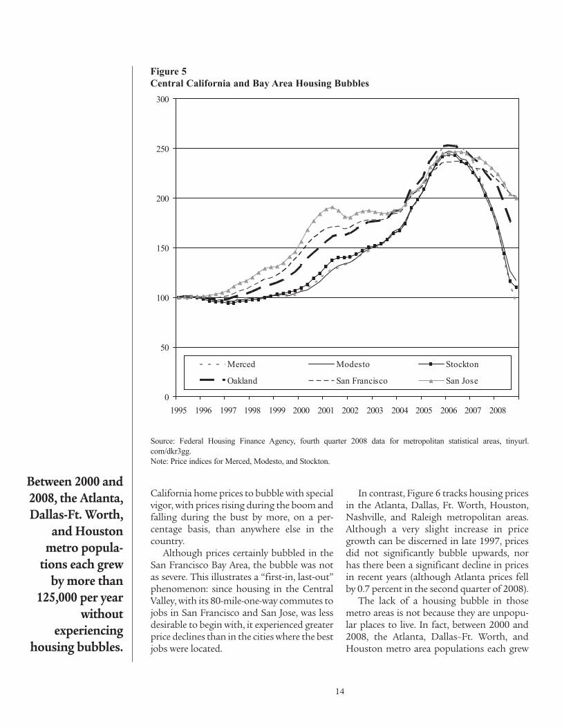
California home prices to bubble with specialvigor, with prices rising during the boom andfalling during the bust by more, on a per-centage basis, than anywhere else in thecountry.

Although prices certainly bubbled in theSan Francisco Bay Area, the bubble was notas severe. This illustrates a “first-in, last-out”phenomenon: since housing in the CentralValley, with its 80-mile-one-way commutes tojobs in San Francisco and San Jose, was lessdesirable to begin with, it experienced greaterprice declines than in the cities where the bestjobs were located.

In contrast, Figure 6 tracks housing pricesin the Atlanta, Dallas, Ft. Worth, Houston,Nashville, and Raleigh metropolitan areas.Although a very slight increase in pricegrowth can be discerned in late 1997, pricesdid not significantly bubble upwards, norhas there been a significant decline in pricesin recent years (although Atlanta prices fellby 0.7 percent in the second quarter of 2008).

The lack of a housing bubble in thosemetro areas is not because they are unpopu-lar places to live. In fact, between 2000 and2008, the Atlanta, Dallas–Ft. Worth, andHouston metro area populations each grew

14

Between 2000 and2008, the Atlanta,Dallas-Ft. Worth,

and Houstonmetro popula-tions each grewby more than

125,000 per yearwithout

experiencinghousing bubbles.

0

50

100

150

200

250

300

1995 1996 1997 1998 1999 2000 2001 2002 2003 2004 2005 2006 2007 2008

Merced Modesto Stockton

Oakland San Francisco San Jose

Figure 5

Central California and Bay Area Housing Bubbles

Source: Federal Housing Finance Agency, fourth quarter 2008 data for metropolitan statistical areas, tinyurl.

com/dkr3gg.

Note: Price indices for Merced, Modesto, and Stockton.


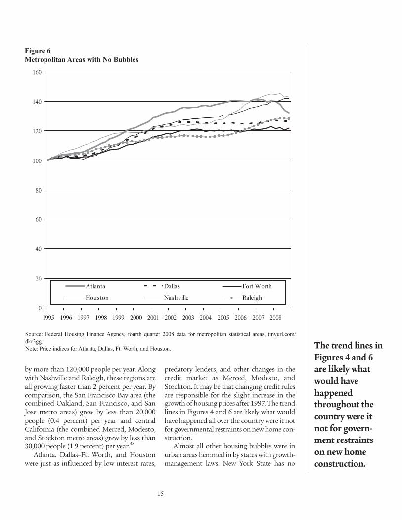
by more than 120,000 people per year. Alongwith Nashville and Raleigh, these regions areall growing faster than 2 percent per year. Bycomparison, the San Francisco Bay area (thecombined Oakland, San Francisco, and SanJose metro areas) grew by less than 20,000people (0.4 percent) per year and centralCalifornia (the combined Merced, Modesto,and Stockton metro areas) grew by less than30,000 people (1.9 percent) per year.48

Atlanta, Dallas–Ft. Worth, and Houstonwere just as influenced by low interest rates,

predatory lenders, and other changes in thecredit market as Merced, Modesto, andStockton. It may be that changing credit rulesare responsible for the slight increase in thegrowth of housing prices after 1997. The trendlines in Figures 4 and 6 are likely what wouldhave happened all over the country were it notfor governmental restraints on new home con-struction.

Almost all other housing bubbles were inurban areas hemmed in by states with growth-management laws. New York State has no

15

The trend lines inFigures 4 and 6are likely whatwould have happenedthroughout thecountry were itnot for govern-ment restraintson new homeconstruction.

0

20

40

60

80

100

120

140

160

1995 1996 1997 1998 1999 2000 2001 2002 2003 2004 2005 2006 2007 2008

Atlanta Dallas Fort Worth

Houston Nashville Raleigh

Figure 6

Metropolitan Areas with No Bubbles

Source: Federal Housing Finance Agency, fourth quarter 2008 data for metropolitan statistical areas, tinyurl.com/

dkr3gg.

Note: Price indices for Atlanta, Dallas, Ft. Worth, and Houston.


such law, and most of its urban areas did notexperience bubbles. But New York City and itsimmediate suburbs (Poughkeepsie, Nassau-Suffolk) did, as their expansion is partly con-trolled by Connecticut and New Jersey.Similarly, Washington, DC, is bordered byMaryland, which has a state growth-manage-ment law, and Virginia, whose northern coun-ties have imposed large-lot zoning to preventurban expansion into rural areas.

Bubbles—prices growing more than 45 per-cent and then declining more than 5 percent—took place in 115, or 30 percent, of the nation’s384 metro areas. Those areas house 46 percentof the metropolitan population.49 All but ahandful of these were in states that were sub-ject to some form of growth management. Thefew that were not, such as Myrtle Beach, SouthCarolina, and Wilmington, North Carolina,may have had some local growth-managementprograms.50

No-bubble metro areas numbered 245 andinclude 50 percent of metro area residents.Only a handful of these, such as Salem andCorvallis, Oregon, and Longview, Washington,were in states that had some form of growthmanagement. Most regions that saw pricesdecline by more than 10 percent are inMichigan, and this is due to the auto indus-tries’ troubles, not to a housing bubble.

The remaining 24 urban areas are in theambiguous category and include a mixture ofareas with and without growth management.Prices in growth-managed Charleston, SouthCarolina, and Missoula, Montana, for exam-ple, increased more than 50 percent but onlydeclined by a little more than 4 percent. Largerdeclines are likely in those areas before the mar-ket bottoms out. On the other hand, prices inunregulated Casper, Wyoming, and Midland,Texas, grew by around 70 percent and havehardly declined. Those cities’ economies arebased on fossil fuel production, which steppedup after 2004 with the increase in oil prices.

In short, there is a very close correlationbetween regions with growth-managementplanning and regions that have seen a majorhousing bubble. Without growth manage-ment, prices in a few parts of the country,

such as Casper and Midland, would havegrown because of local factors; and prices inother parts, such as Michigan, would havedeclined because of local factors.

In most of the country, however, priceswithout growth management would havelooked like those in Figures 4 or 6. There mighthave been some subprime mortgage defaults—particularly in Michigan—but there wouldhave been no major housing bubbles, no cred-it crisis, no need for a bank bailout, and noworldwide recession.

Housing Bubbles inOther Countries

The United States is not the only countrywhose planners use growth-management tools,and it is not the only country to have a housingbubble. “Two thirds (by economic weight) of theworld . . . has a potential housing bubble,”observed The Economist in 2004.51 Great Britainhas used growth management since 1947, and itunderwent a severe housing bubble. Much ofcontinental Europe, Australia, and New Zealandhave similar land-use policies and also have hadhousing bubbles.

Vincent Benard, of l’Institut Hayek, ob-serves that French land-use authorities writeplans every 10 to 15 years. If there is a surge indemand between the rewrites, the plans mayfail to have enough land available to accom-modate new development. A six-year permit-ting process further contributes to long lagsbetween new demand and the time home-builders can meet that demand. As a result,land-use regulations “appeared to be, by far,the main factor explaining” the French hous-ing bubble.52

Canada, like the United States, does nothave a national land-use policy. But someurban areas, notably Vancouver and Toronto,practice growth management. These tworegions have the most expensive housing inthe nation, with a typical home in Vancouvercosting four times as much as a similar homein Ottawa, the nation’s capital, and five timesas much as a similar home in Montreal.53

16

French economistVincent Benard

says that land-useregulations

“appeared to be,by far, the main

factor explaining”the housing

bubble in France.


Vancouver home prices peaked in 2007 anddeclined by 10 percent in 2008.54

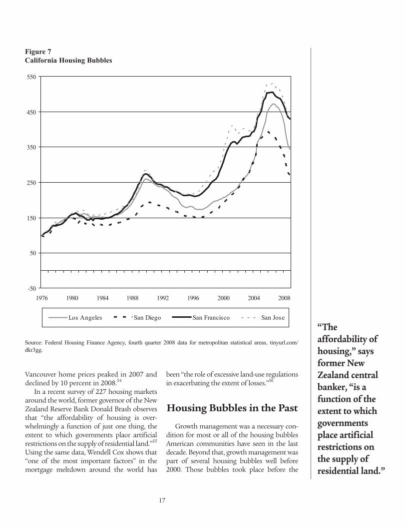
In a recent survey of 227 housing marketsaround the world, former governor of the NewZealand Reserve Bank Donald Brash observesthat “the affordability of housing is over-whelmingly a function of just one thing, theextent to which governments place artificialrestrictions on the supply of residential land.”55

Using the same data, Wendell Cox shows that“one of the most important factors” in themortgage meltdown around the world has

been “the role of excessive land-use regulationsin exacerbating the extent of losses.”56

Housing Bubbles in the Past

Growth management was a necessary con-dition for most or all of the housing bubblesAmerican communities have seen in the lastdecade. Beyond that, growth management waspart of several housing bubbles well before2000. Those bubbles took place before the

17

“The affordability ofhousing,” saysformer NewZealand centralbanker, “is afunction of theextent to whichgovernmentsplace artificialrestrictions onthe supply of residential land.”

-50

50

150

250

350

450

550

1976 1980 1984 1988 1992 1996 2000 2004 2008

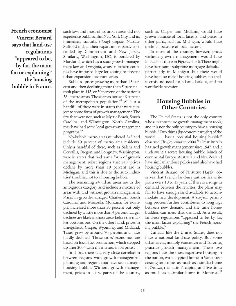
Los Angeles San Diego San Francisco San Jose

Figure 7

California Housing Bubbles

Source: Federal Housing Finance Agency, fourth quarter 2008 data for metropolitan statistical areas, tinyurl.com/

dkr3gg.


loosening of credit that many claim caused therecent bubble. The difference between earlierbubbles and the recent one is that fewer stateswere practicing growth management in earlierdecades, and so a much smaller share ofAmerican housing suffered from such bubbles.

Figure 7 shows two earlier bubbles in the LosAngeles, San Diego, San Jose, and San Franciscometropolitan areas. The first was when pricesgrew in the late 1970s in response to the origi-nal imposition of urban-growth boundaries.Prices fell in the early 1980s. Then prices bub-bled again, peaking in 1990 and crashing againthrough 1995. Silicon Valley suffered a smallbubble that peaked in 2001, but this was reallyjust a part of the most recent bubble.

Again, there is a close correlation betweenbubbles and growth management. The bubblethat peaked in 1980 took place in California,Hawaii, Oregon, and Vermont—the only statesthat were practicing growth management inthe 1970s. By the 1980s, several New Englandstates and a few urban areas, including Seattle,began practicing growth management, andthey joined in the bubble that peaked in 1990.Few, if any, states or urban areas that were notpracticing growth management had housingbubbles before 2000.

Foreign countries that practice growthmanagement have also had previous bubbles.Norway, Sweden, and Finland had propertybubbles that peaked in 1990 and were severeenough to send virtually all of the nations’banks into bankruptcy.57 Japanese policiesaimed at preventing the development of rur-al land included 150 percent capital gainstaxes on short-term property gains.58 Theresulting property bubble and inevitable col-lapse led to a decade-long recession.

Several studies have tied volatility to land-use regulation. A 2005 economic analysis ofthe housing market in Great Britain, whichhas practiced growth management since 1947,found that planning makes housing marketsmore volatile. “By ignoring the role of supplyin determining house prices,” the report says,“planners have created a system that has lednot only to higher house prices but also to ahighly volatile housing market.”59

Economists Edward Glaeser and JosephGyourko have found similar results in theUnited States. Land-use rules that restrict“housing supply lead to greater volatility inhousing prices,” they say, adding that, “if anarea has a $10,000 increase in housing pricesduring one period, relative to national andregional trends, that area will lose $3,300 inhousing value over the next five-year peri-od.”60 Both the Great Britain and the Glaeser-Gyourko studies were based on data preced-ing the current housing bubble.

Responding toUnaffordability

Because prices do not decline as much incrashes as they increase in booms, successivebubbles can make housing grotesquely unaf-fordable. In 1969, the nation’s least-afford-able metropolitan area, with a median-home-value-to-median-family-income ratio of 3.2,was Honolulu, mainly because of Hawaii’s1961 growth-management law. As previouslynoted, most other metropolitan areas hadratios of 1.5 to 2.5.

By 1979, after Oregon and California hadimplemented growth management plans, theHonolulu value-to-income ratio was 5.5, atwhich point it became virtually impossiblefor a median family to get a mortgage on amedian home given the terms typical of theday. In much of California, 1979 value-to-income ratios were between 4 and 5, whilethey had reached 3.2 (Honolulu’s 1969 ratio)in some Oregon communities.

Despite the decline in real California andHawaii home prices in the early 1980s, the late-1980s bubble pushed California value-to-in-come ratios to as high as 6.7 in San Francisco(compared with 6.2 in Honolulu) and well above4 in much of the rest of California. This bubblealso pushed prices in Boston, New York, andnearby metro areas above 4. Oregon, which suf-fered a greater recession in the early 1980s thanmost states, did not have a late-1980s bubble.

Prices in California, Hawaii, and the North-east crashed in the early 1990s, but by 1999

18

Land-use restrictions not

only make housing

unaffordable,they make pricesmore volatile.


value-to-income ratios had recovered and werepoised for another leap. By 2006, price-to-income ratios throughout California andHawaii ranged from 5 to as high as 11.5. Inresponse to growth-management plans writ-ten in the mid- to late-1990s, value-to-incomeratios in Arizona, Florida, Maryland, andWashington ranged from 3 to 5.5.

The pattern is clear: each successive bubblepushes value-to-income ratios further awayfrom the natural ratio of about 2.0. Even at thebottom of the cycle in 1995, many Californiavalue-to-income ratios were well above 5,meaning that housing was still unaffordabledespite the crash of the early 1990s.

Much media attention has focused on theCommunity Reinvestment Act of 1977 andits role in encouraging banks to make riskyloans to low-income families. Just as impor-tant is how the Department of Housing andUrban Development responded to the grow-ing housing affordability crisis by encourag-ing banks to loosen their criteria for makingloans to moderate-income families that werepriced out of housing markets by growth-management planning.

In 1992, Congress gave the Department ofHousing and Urban Development the respon-sibility for regulating Fannie Mae and FreddieMac (collectively known as government-spon-sored enterprises, or GSEs) to ensure that theydid not engage in risky behavior. But this con-flicted with HUD’s primary mission, which “isto increase homeownership, support commu-nity development, and increase access to afford-able housing free from discrimination.”61

As successive HUD secretaries becameaware of housing affordability problems inCalifornia and other parts of the country,they used their regulatory authority to orderthe GSEs to buy more loans from “low- andmoderate-income families.” Specifically, in1995, Secretary Henry Cisneros ordered thatat least 42 percent of the mortgages pur-chased by the GSEs had to be from low- andmoderate-income families. In 2000, SecretaryAndrew Cuomo increased this to 50 per-cent.62 In 2004, Secretary Alphonso Jacksonincreased it yet again to 58 percent.63

One response to these rules was an increasein Fannie Mae and Freddie Mac purchases ofsubprime loans, meaning loans made to peo-ple with poor credit histories. But anotherresponse was to relax the loan criteria forprime loans, that is, loans to people with excel-lent credit histories who nonetheless had ahard time buying houses in unaffordablestates like California. Before 1995, Fannie Maeand Freddie Mac would normally buy only 15-to 30-year mortgages with at least 10 percentdown and monthly payments (plus insuranceand property taxes) that were no more thanabout 33 percent of the homebuyer’s income.

When brand-new starter homes cost$110,000, as they do in Houston, a 10 percentdown payment is not a formidable obstacle.When starter homes cost closer to $400,000, asthey did in the San Francisco Bay Area in thelate-1990s, the obstacle is much greater. Value-to-income ratios of 5 and above require 40- to50-year payment periods and/or mortgages thatcost more than 33 percent of a family’s income.

The result was that mortgage companiesgreatly reduced the criteria required to getloans. They no longer required 10 percentdown payments. People could get loans for 40and even 50 years. And borrowers could dedi-cate well over half their incomes to their mort-gages. These changes allowed people to buyhomes that were five or six times their incomes,but they also increased the risks of defaultseven among supposedly prime borrowers.

Such regulatory actions would not havebeen necessary if growth management had notmade a substantial portion of American hous-ing unaffordable. While urban planners hadnothing to do with credit default swaps or oth-er derivatives, they are directly responsible forunaffordable housing and indirectly responsi-ble for the government’s loosening of creditstandards in response to that unaffordability.

Should GovernmentStabilize Home Prices?

When financial markets melted down inOctober 2008, several economists argued that

19

By eliminatingthe requirementthat homebuyersmake at least a 10 percent down-payment, FannieMae and FreddieMac increased therisk of defaults.


the solution was to “stabilize home prices.”64 InFebruary 2009, President Obama announced aplan that aimed to “shore up housing prices”and “arrest this downward spiral.”65 Whenpotential homeowners refuse to buy homesuntil the market bottoms out, it is easy to seewhy some people might think that the problemwith the nation’s housing markets is fallingprices.

Yet the reality is that—in terms of median-home-price-to-median-income ratios—housingremains much too expensive in virtually all ofthe bubble markets. Such expensive housingputs hardships on consumers, and as Portlandeconomist Randall Pozdena notes, those hard-ships fall hardest on poor, minority, and work-ing-class families.66 The benefits gained byhomesellers who earn windfall profits becauseof artificial housing shortages are unfair becauseexisting homeowners tend to be wealthier thanfirst-time home buyers. Moreover, those bene-fits do not entirely offset the costs, some ofwhich, such as the cost of an onerous permittingprocess, are simply deadweight losses to society.

Furthermore, housing is only one symp-tom of the problems created by growth-man-agement policies. Such policies impose thesame sorts of hardships on businesses thatneed land and structures for offices, facto-ries, stores, and other purposes.

Glaeser and Gyourko agree that an effortto stabilize housing prices is a bad idea. Theypoint out that most of the tools governmentwould use to support housing prices, such as

reduced interest rates or more favorable loans,would be extremely costly yet have only mar-ginal and uncertain effects on housing. “Thisis a bad combination,” they dryly observe.67

The biggest reason to oppose price stabi-lization is that it contradicts other governmentpolicies. “Housing affordability has long been astated goal of the federal government,” Glaeserand Gyourko point out. “Why should it nowtry to make it more difficult for people to buy,or rent, a home by supporting prices?”68 Thereal problem, they add, “is not the price declinebut the previous price explosion.”69

Of course, the reason housing prices arehigh in most areas that suffered housing bub-bles is because of explicit government policiesaimed at discouraging construction of newsingle-family homes. Rightly or wrongly, highhousing prices serve this agenda, so govern-ment efforts to promote homeownership areundermined by other government efforts todiscourage it.

As an alternative, “home prices must get backto pre-bubble levels,” suggests Harvard econo-mist Martin Feldstein. But, he adds, “Congressshould enact policies to reduce defaults thatcould drive prices down much further.”70 Yetsuch policies carry the same perils as efforts tostabilize prices—especially since pre-bubbleprices in several states and urban areas werealready well above normal value-to-incomeratios.

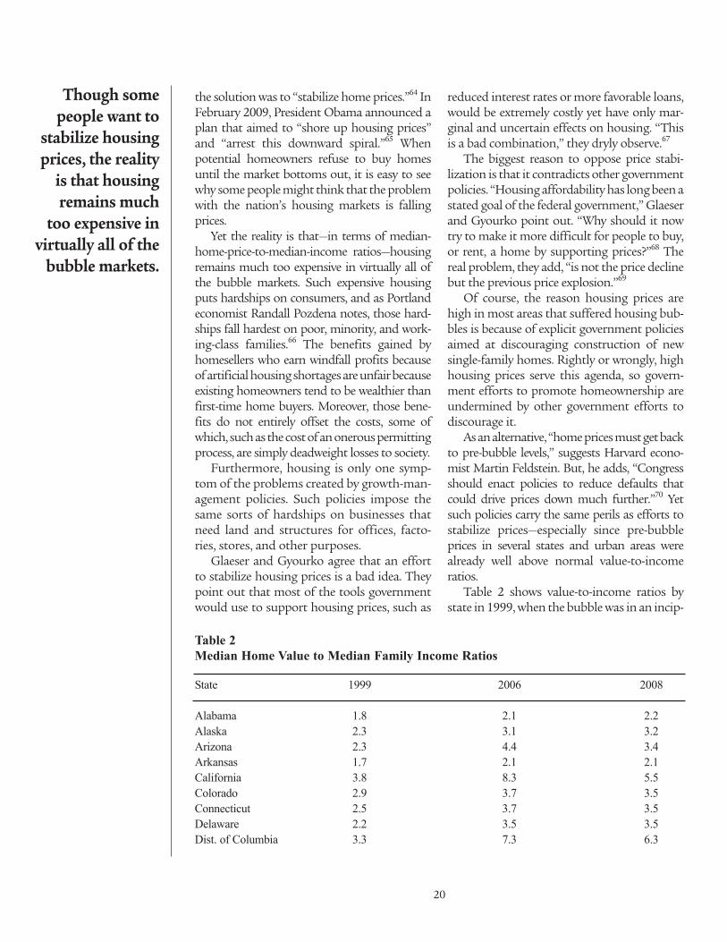
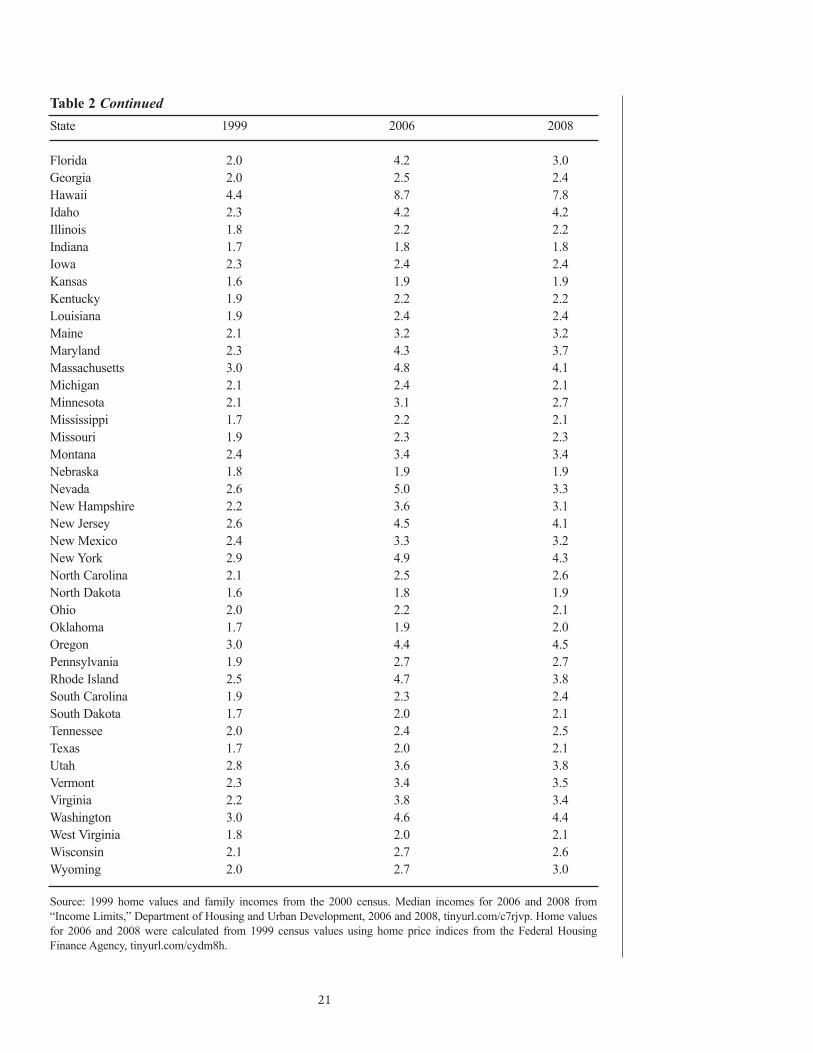
Table 2 shows value-to-income ratios bystate in 1999, when the bubble was in an incip-

20

Though somepeople want to

stabilize housingprices, the realityis that housingremains muchtoo expensive in virtually all of thebubble markets.

Table 2

Median Home Value to Median Family Income Ratios

State 1999 2006 2008

Alabama 1.8 2.1 2.2

Alaska 2.3 3.1 3.2

Arizona 2.3 4.4 3.4

Arkansas 1.7 2.1 2.1

California 3.8 8.3 5.5

Colorado 2.9 3.7 3.5

Connecticut 2.5 3.7 3.5

Delaware 2.2 3.5 3.5

Dist. of Columbia 3.3 7.3 6.3


21

Table 2 Continued

State 1999 2006 2008

Florida 2.0 4.2 3.0

Georgia 2.0 2.5 2.4

Hawaii 4.4 8.7 7.8

Idaho 2.3 4.2 4.2

Illinois 1.8 2.2 2.2

Indiana 1.7 1.8 1.8

Iowa 2.3 2.4 2.4

Kansas 1.6 1.9 1.9

Kentucky 1.9 2.2 2.2

Louisiana 1.9 2.4 2.4

Maine 2.1 3.2 3.2

Maryland 2.3 4.3 3.7

Massachusetts 3.0 4.8 4.1

Michigan 2.1 2.4 2.1

Minnesota 2.1 3.1 2.7

Mississippi 1.7 2.2 2.1

Missouri 1.9 2.3 2.3

Montana 2.4 3.4 3.4

Nebraska 1.8 1.9 1.9

Nevada 2.6 5.0 3.3

New Hampshire 2.2 3.6 3.1

New Jersey 2.6 4.5 4.1

New Mexico 2.4 3.3 3.2

New York 2.9 4.9 4.3

North Carolina 2.1 2.5 2.6

North Dakota 1.6 1.8 1.9

Ohio 2.0 2.2 2.1

Oklahoma 1.7 1.9 2.0

Oregon 3.0 4.4 4.5

Pennsylvania 1.9 2.7 2.7

Rhode Island 2.5 4.7 3.8

South Carolina 1.9 2.3 2.4

South Dakota 1.7 2.0 2.1

Tennessee 2.0 2.4 2.5

Texas 1.7 2.0 2.1

Utah 2.8 3.6 3.8

Vermont 2.3 3.4 3.5

Virginia 2.2 3.8 3.4

Washington 3.0 4.6 4.4

West Virginia 1.8 2.0 2.1

Wisconsin 2.1 2.7 2.6

Wyoming 2.0 2.7 3.0

Source: 1999 home values and family incomes from the 2000 census. Median incomes for 2006 and 2008 from

“Income Limits,” Department of Housing and Urban Development, 2006 and 2008, tinyurl.com/c7rjvp. Home values

for 2006 and 2008 were calculated from 1999 census values using home price indices from the Federal Housing

Finance Agency, tinyurl.com/cydm8h.


ient stage; 2006, when it reached its peak inmany places; and the last quarter of 2008. In1999, only 4 states had average value-to-income ratios of three or more, and only 1state was greater than four. By 2006, home val-ues in 24 states were three times incomes and13 states were greater than four. As of the lastquarter of 2008, values in 24 states were still atleast three times median incomes and eightstates were greater than four. So prices stillhave to fall to get back to 1999 levels of afford-ability, and in a few states they should fall evenfurther to value-to-income ratios lower thanthree.

Planners argue that growth managementhelps preserve open space and reduces theamount of driving people need to do. Yet theshare of U.S. land that would be protectedfrom urbanization through denser housing isminiscule—probably less than 1 percent—andthe effects of density on driving are also small.

The negative effects of growth manage-ment—on housing prices, on the costs of doingbusiness, on congestion, and on personal liber-ty—are far greater than the benefits, most ofwhich can be achieved in other ways at a far low-er cost. Rather than prop up housing prices,then, the current recession is an excellent time tostart the discussion of how housing prices inareas with growth management can be returnedto normal, affordable levels.

Planners’ Response

Many urban planners steadfastly deny thattheir growth-management policies makehousing more expensive. Instead, they claimthat higher-priced housing is solely due toincreased demand resulting from the quality-of-life improvements resulting from their poli-cies. As Paul Danish, the city council memberwhose plans made Boulder, Colorado, hous-ing less affordable than 90 percent of the oth-er urban areas in the United States, says,Boulder housing prices are high solely becauseit is “a really desirable place to live,” while any-where else with lower prices is “a really awfulplace to live.”71

In reality, housing bubbles are solely due tosupply problems. When the supply of newhomes is elastic, an increase in demand shouldnot result in a significant increase in price.There are several reasons why supply may beinelastic, but most of them relate to land-useregulation or other government policies thatkeep land unavailable for housing. Preventingfuture housing bubbles and the economicinstability they cause will require dismantlingthose growth-management policies.

Ironically, many planning advocates areusing declining home prices as an argumentin favor of more growth-management plan-ning. They observe that most of the house-holds in the high-density housing projectsfavored by smart-growth plans have no chil-dren, and that an increasing share of Americanhouseholds is childless. They therefore reasonthat the share of households that want single-family homes is about to decline drastically,and the recent drop in housing prices is asymptom of that decline.

A prime example is Arthur Nelson, an urbanplanning professor at the University of Utah,whose projection of 22 million “surplus” sub-urban homes by 2025 was cited in Time andAtlantic Monthly. That projection is based on atable in a paper by Nelson titled “Summary ofHousing Preference Survey Results.” The tablesays that 38 percent of Americans prefer multi-family housing, 37 percent prefer homes onsmall (less than one-sixth acre) lots, and 25 per-cent prefer homes on large lots. A note to thetable says it “is based on interpretations of sur-veys by Myers and Gearin (2001).”72

However, Myers and Gearin’s paper, whichreviews surveys of housing preferences, hardlysupports Nelson’s table. “Americans over-whelmingly prefer a single-family home on alarge lot,” concludes one survey they cite.Others found that “83 percent of respondentsin the 1999 National Association of HomeBuilders Smart Growth Survey prefer a single-family detached home in the suburbs”; “74 per-cent of respondents in the 1998 VermontersAttitudes on Sprawl Survey preferred a homein an outlying area with a larger lot”; and “73percent of the 1995 American Lives New

22

Housing bubblesare due solely tosupply problems,not to changes inhousing demand.


Urbanism Study respondents prefer suburbandevelopments with large lots.”73

Indeed, the main point of Myers andGearin’s article is not that most Americanswant to live on small lots or in multifamilyhomes, but only that there is a contingent ofAmericans who do prefer such housing. “Somehousing consumers actually prefer higher den-sity,” they report.74 They also speculate thatpeople are more likely to join that group asthey get older. However, their evidence for thisis sketchy: surveys showing that older peopleare “receptive to decreased auto dependence.”75

Being “receptive” is far from choosing to live inhigher densities; the same Vermont survey thatreported 74 percent of people want to live on alarge lot found that 48 percent want to be with-in walking distance of stores and services.76

These two preferences are incompatible, andmost Americans have picked the large lot overwalking distance to stores.

The information used by Nelson “may notbe terribly reliable,” comments Emil Malizia, aplanning professor at the University of NorthCarolina. “The samples are self-selected” hesays, “the responses may be heavily influencedby the data collection method,” and “peopleoften do not behave in ways that are consis-tent with the preferences or opinions theyexpress.”77

So the claim that the nation will soon havea huge surplus of large-lot homes is based on,at best, a misinterpretation of the data. Nelsonuses this misinterpretation to urge planners todesign a new “template” for future develop-ment and redevelopment that focuses onhigher densities and mixed-use develop-ments.78 In short, Nelson promotes his erro-neous data to justify growth-managementpolicies that will increase the scarcity of single-family homes despite the reality that these arethe homes most Americans prefer.

The Next Housing Bubble

The prime cause of the housing bubble thatgenerated the recent financial crisis was over-regulation of land that created artificial short-

ages of housing. Over the last decade, housingprices have bubbled in almost every state andregion that has attempted to regulate growth,while very few areas that haven’t practicedgrowth management have seen housing pricesrise and crash. Prices have also bubbled in oth-er countries with managed growth policies, aswell as in past decades in the few states thatattempted to manage growth before 1990.

Understanding that growth managementcaused the housing bubble that led to therecent economic crisis provides little help insolving the crisis. But it can help in prevent-ing future housing bubbles and economiccrises.

As previously noted, Tennessee passed agrowth-management law in 1998 but did notexperience a housing bubble. In the next eco-nomic boom, however, Tennessee is likely tojoin the bubble club. So will any other statesthat are persuaded by local chapters of theAmerican Planning Association to pass similarlaws. The APA has written “model statutes” forsuch planning as well as a guidebook to helpplanners generate “grassroots support” forlaws that give them more power to managegrowth.79

On top of this, the California legislaturerecently passed a bill mandating even strictergrowth management on the unproven (andunlikely) premise that ever-denser housingwill reduce greenhouse gas emissions.80 Thisbill is regarded as a model for other states andsome in Congress have proposed to incorpo-rate some of its concepts into federal law.

If present trends continue, then, the nexthousing bubble is likely to affect an evengreater percentage of American housing. It isalso likely to push value-to-income ratios evenhigher, with ratios reaching 14 or 15 in the SanFrancisco Bay Area, 10 in much of the rest ofCalifornia, and 6 or more in Florida and otherstates that experienced their first bubble in thelast decade.

If problems with derivatives are fixed, thenext housing bubble might not cause an inter-national financial meltdown. Yet, as EdwardChancellor observes in Devil Take the Hindmost,“speculation demands continuing govern-

23

Despite the relationshipbetween growthmanagement andhousing bubbles,the AmericanPlanningAssociation isurging morestates to passsuch laws.


ment restrictions, but inevitably it will breakany chains and run amok.”81 Even if the nextbubble does not cause an international crisis,it will impose severe hardships on homebuy-ers, turn ordinarily stable regions into boom-bust economies, increase the costs to business-es, and greatly restrict personal choice andfreedom.

It will also greatly transform urban areas,and not for the better. As Joel Kotkin has docu-mented, while low-cost housing markets main-tain a diversity of incomes, lower- and middle-income people are migrating away from SanFrancisco and other high-cost markets.82 This isturning these places, says one demographer,into “Disneylands for yuppies.”83 Some couldargue that this helps to create a diverse array ofcommunities, but the alternative view (asexpressed by Glaeser) is that it makes the affect-ed regions “less diverse” and turns them into“boutique cities catering only to a small, highlyeducated elite.”84

Conclusions

Housing bubbles triggered the financialmeltdown of 2008. Those bubbles did notresult from low interest rates, changes inmortgage requirements, or other factors influ-encing demand. Instead, a necessary conditionfor their formation was supply shortages,most of which resulted from urban plannersengaged in what they considered to be state-of-the-art growth-management planning. TheUnited States is fortunate that they were ableto practice these policies in only about 16states, else the costs of the financial crisiswould be even greater.

The best thing the government can do isallow home prices to fall to market levels. Todo this, states and urban areas with growth-management laws and plans should repealthose laws and dismantle the programs thatmade housing expensive in the first place.This will obviously be easier to do in stateslike Florida, where value-to-income ratioshave returned to affordable levels, than inCalifornia, where housing remains unafford-

able. But repealing California’s grotesqueplanning laws will probably help kick-startits economy, which in many respects is ineven worse shape than Michigan’s.

States and regions that have been consider-ing growth-management laws and plansshould firmly reject them. Both Congress andthe states should reject proposals to imposeCalifornia-style policies aimed at creatingmore compact cities, supposedly to reduce dri-ving and greenhouse gas emissions. The costsof such policies will be extremely high andtheir beneficial effects will be negligible.

Bubbles and credit crises happen too oftenas it is. Governments should not increase theirfrequencies and depths by creating artificialhousing and real estate shortages.

Notes1. Nell Henderson, “Bernanke: There’s No HousingBubble to Go Bust,” Washington Post, October 27,2005, p. D1, tinyurl.com/85v9s.

2. Paul Krugman, “That Hissing Sound,” NewYork Times, August 8, 2005, tinyurl.com/9lwmp.

3. Harvey Mansfield, “A Question for the Econo-mists: Is the Overly Predicted Life Worth Living?”Weekly Standard, April 13, 2009, tinyurl.com/dkfuhz.

4. Pam Woodall, “House of Cards,” The Economist,May 29, 2003.

5. “The Global Housing Boom,” The Economist,June 16, 2005.

6. “After the Fall,” The Economist, June 16, 2005.

7. David Henderson, “Don’t Blame Greenspan,”Wall Street Journal, March 26, 2009, tinyurl.com/ddjhvc.

8. Judy Shelton, “Loose Money and the DerivativeBubble,” Wall Street Journal, March 26, 2009, tinyurl.com/ddjhvc.

9. Peter J. Wallison, “The True Origins on theFinancial Crisis,” American Spectator, February 2009,tinyurl.com/bzh64s.

10. Bryan Walsh, “Recycling the Suburbs,” Time,March 12, 2009, tinyurl.com/b447yn.

11. Christopher B. Leinberger, “The Next Slum?”

24

While low-costhousing markets

maintain a diversity ofincomes, lower- and

middle-incomepeople are

migrating awayfrom high-cost

markets.


Atlantic Monthly, March 2008, tinyurl.com/2cmrfd.

12. “Recession-Plagued Nation Demands NewBubble to Invest In,” The Onion, July 14, 2008,tinyurl.com/5jgfha.

13. Ronald R. King, Vernon L. Smith, Arlington W.Williams, and Mark van Boening, “The Robustnessof Bubbles and Crashes in Experimental StockMarkets,” in R. H. Day and P. Chen, Nonlinear Dy-namics and Evolutionary Economics (Oxford, England:Oxford University Press, 1993).

14. Charles Kindleberger and Robert Aliber, Manias,Panics, and Crashes: A History of Financial Crises, 5th ed.(Hoboken, NJ: Wiley, 2005), pp. 25–33.

15. Eric A. Hanushek and John M. Quigley, “WhatIs the Price Elasticity of Housing Demand?” TheReview of Economics and Statistics 62, no. 3: 449–54,tinyurl.com/766wq.

16. National Family Opinion, Consumers SurveyConducted by NAR and NAHB (Washington:National Association of Realtors, 2002), p. 6.

17. Royal Bank of Canada, 2007 HomeownershipSurvey (Toronto, ON: Royal Bank of Canada, 2007),p. 13, tinyurl.com/2wu7cp.

18. “Urban/Rural and Inside/Outside Metropoli-tan Area, GCT-PH1. Population, Housing Units,Area, and Density: 2000,” Census Bureau, tinyurl.com/5b7acg.

19. National Resources Conservation Service,National Resources Inventory—2003 Annual NRI(Washington: Natural Resources ConservationService, 2006), p. 1, tinyurl.com/62fnxf.

20. William Bogart, Don’t Call It Sprawl: MetropolitanStructure in the 21st Century (New York: CambridgeUniversity Press, 2006), p. 7.

21. “Home Values,” National Association of Real-tors, 2008, tinyurl.com/5dtd2v.

22. 1970 Census of Housing, Volume 1, HousingCharacteristics for States, Cities, and Counties, Part 1,United States Summary, table 17, “Financial Char-acteristics for Areas and Places; 1970 Census of thePopulation, Volume 1, Characteristics of the Population,Part 1, United States Summary, Section 2, table 366,“Median Income in 1969 of Families by Type ofFamily and Race of Head for Standard Metropoli-tan Statistical Areas of 250,000 or More.”

23. Hawaii State Land Use Law (Hawaii RevisedStatutes, chapter 205).

24. Bernard Siegen, Land Use without Zoning

(Lanham, MD: Lexington Books, 1972), p. 33.

25. “Metropolitan and Micropolitan StatisticalArea Population and Estimated Components ofChange: April 1, 2000 to July 1, 2008,” Census Bu-reau, 2009, tinyurl.com/cs6344.

26. “Home Price Comparison Index,” ColdwellBanker, 2008, tinyurl.com/2t8smh.

27. Greenbelt Alliance, At Risk: The Bay Area Green-belt (San Francisco, CA: Greenbelt Alliance, 2006),p. 4, tinyurl.com/ys3d4n.

28. Scott Adams, “The Economy Again,” TheDilbert Blog, March 4, 2009, tinyurl.com/cg2rzu.

29. Sharon Simonson, “Developers Drop CoyoteValley Housing Plans,” San Jose Business Journal,March 18, 2008, tinyurl.com/dk45kb.

30. Eric Freyfogle, The Land We Share: Private Propertyand the Common Good (Washington: Island Press,2003), p. 219.

31. Carol N. Doty v. Coos County, Oregon Courtof Appeals, 2001-202, tinyurl.com/c37bog.

32. David E. Dowall, The Suburban Squeeze: LandConservation and Regulation in the San Francisco BayArea (Berkeley, CA: University of California Press,1984), pp. 141–42.

33. Tracey Kaplan and Sue McAllister, “Cost ofLand Drives Home Prices,” San Jose Mercury News,August 4, 2002.

34. Tom Means, Edward Stringham, and EdwardLopez, “Below-Market Housing Mandates asTakings: Measuring Their Impact,” IndependentInstitute Policy Report, November, 2007, p. 15,tinyurl.com/6rnugn.

35. Jonathan Brinckman, “Arbor Homes Dominateas Urban-Growth Limits Keep National Devel-opers at Bay,” Oregonian, September 1, 2005.

36. Joe Hurd, The Bay Area Economy: The MeltdownIsn’t Over (University of California, Los Angeles,2003), page 4.4.

37. Randal O’Toole, “The Planning Tax: The Caseagainst Regional Growth-Management Planning,”Cato Policy Analysis no. 606, December 6, 2007, p. 5.

38. “Southern Nevada Public Land ManagementAct of 1998,” Bureau of Land Management, 2009,tinyurl.com/d54txm.

39. Jesse McKinley, “Nevada Learns to Cash In on

25


Sales of Federal Land,” New York Times, December3, 2007, tinyurl.com/cwbodd.

40. Andre Leventis, “A Note on the Differencesbetween the OFHEO and S&P/Case-Shiller HousePrice Indices,” Federal Housing Finance Agency,2007.

41. All references to home prices by state are basedon “Fourth Quarter 2008 Home Price Index Datafor Individual States,” Federal Housing FinanceAgency, 2009, tinyurl.com/cb72o7.

42. All adjustments for inflation were made using“Current Dollar and ‘Real’ Gross Domestic Prod-uct,” Bureau of Economic Analysis, 2009, tinyurl.com/ad629c.

43. “Population Estimates,” Census Bureau, 2009,tinyurl.com/cnacq6.

44. A complete data set with all home price indicesand calculations made for this report for all 50states and the District of Columbia can be down-loaded from tinyurl.com/cq6mvo. A spreadsheetsummarizing these data, which is similar to table 1,can be downloaded from tinyurl.com/csqaol.

45. “Foreclosure Activity Decreases 10 Percent inJanuary,” Realtytrac.com, 2009, tinyurl.com/dhnhrr.

46. All references to home prices by metropolitanarea are based on “Fourth Quarter 2008 HomePrice Index Data for Metropolitan StatisticalAreas,” Federal Housing Finance Agency, 2009,tinyurl.com/dkr3gg.

47. For a detailed explanation of how this lawworks, see Randal O’Toole, “Do You Know the Wayto L.A.?” Cato Institute Policy Analysis no. 602,October 17, 2007, pp. 10–13.

48. “Metropolitan and Micropolitan StatisticalArea Population and Estimated Components ofChange: April 1, 2000 to July 1, 2008,” Census Bu-reau, 2009, tinyurl.com/cs6344.

49. Ibid.

50. A complete data set with all home price indicesand calculations made for this report for all 384metropolitan areas can be downloaded fromtinyurl.com/dzuab7 (this file is more than 6megabytes). A spreadsheet summarizing thesedata, showing how much prices have grown andfallen by MSA, can be downloaded from tinyurl.com/cbw4n7.

51. “The Sun Also Sets,” The Economist, September9, 2004.

52. Vincent Benard, “Land-Use Regulations, Hous-ing Unaffordability, and Other Undesirable Im-pacts,” presentation to the 2009 Preserving theAmerican Dream conference, April 18, 2009, Belle-vue, WA.

53. “2007 Home Price Comparison Index,” Cold-well Banker, 2007, tinyurl.com/5grshw.

54. “2008 Home Price Comparison Index,” Cold-well Banker, 2008, tinyurl.com/2t8smh.

55. Wendell Cox, with introduction by DonaldBrash, Fourth Annual Demographia InternationalHousing Affordability Survey: 2008 (Belleville, IL:demographia.com, 2008), p. ii.

56. Wendell Cox, How Smart Growth Exacerbated theInternational Financial Crisis (Washington: HeritageFoundation, 2008), p. 1, tinyurl.com/594mvm.

57. Kindleberger and Aliber, p. 3.

58. Edward Chancellor, Devil Take the Hindmost: AHistory of Financial Speculation (New York: Plume,2000), p. 293.

59. Alan W. Evans and Oliver Marc Hartwich, Un-affordable Housing: Fables and Myths (London, Eng-land: Policy Exchange, 2005), p. 9, tinyurl.com/a4njl.

60. Edward Glaeser, The Economic Impact of Restrict-ing Housing Supply (Cambridge, MA: Rappaport In-stitute, 2006), p. 1, tinyurl.com/6zsovh.

61. Department of Housing and Urban Develop-ment “HUD’s Mission,” Department of Housingand Urban Development, 2003, tinyurl.com/6cy3w7.

62. Wayne Barrett, “Andrew Cuomo and Fannieand Freddie,” Village Voice, August 5, 2008, tinyurl.com/3hl6zo.

63. Carol D. Leonnig, “How HUD Mortgage PolicyFed the Crisis,” Washington Post, June 10, 2008, p.A1, tinyurl.com/3m7cgd.

64. R. Glenn Hubbard and Chris Mayer, “First, Let’sStabilize Home Prices,” Wall Street Journal, Oc-tober2, 2008, tinyurl.com/43m95e; Martin Feldstein,“The Problem Is Still Falling House Prices,” WallStreet Journal, October 4, 2008, tinyurl.com/427lsr.

65. Barack Obama, “Remarks of the President onthe Mortgage Crisis” (speech at the White House,Washington, February 18, 2009), tinyurl.com/ddqsfd.

66. Randal Pozdena, Smart Growth and Its Effects onHousing Markets: The New Segregation (Washington:National Center for Public Policy Research, 2002),

26


p. 40, tinyurl.com/38ybkt.

67. Edward Glaeser and Joseph Gyourko, “TheCase against Housing Price Supports,” Economists’Voice, October, 2008, p. 1, tinyurl.com/6dv92x.

68. Ibid.

69. Ibid., p. 2.

70. Martin Feldstein, “The Stimulus Plan WeNeed Now,” Washington Post, October 30, 2008, p.A23, tinyurl.com/6n7qla.

71. Eric Schmidt, “The Price of Smart Growth,”Boulder Daily Camera, May 21, 2006.

72. Arthur C. Nelson, “Leadership in a New Era,”Journal of the American Planning Association 72, no. 4(2006): 397.

73. Dowell Myers and Elizabeth Gearin, “CurrentPreferences and Future Demand for DenserResidential Environments,” Housing Policy Debate,volume 12 (2001), no. 4, pp. 635–36.

74. Dowell Myers and Elizabeth Gearin, “CurrentPreferences and Future Demand for DenserResidential Environments,” Housing Policy Debate12, no. 4 (2001): 638.

75. Ibid., p. 642.

76. Ibid., p. 638.

77. Emil Malizia, “Comment on ‘Leadership in aNew Era,’” Journal of the American Planning Associ-ation 72, no. 4 (2006): 407.

78. Arthur C. Nelson and Robert Lang, “The Next100 Million,” American Planning Association, 2007,p. 5, tinyurl.com/cd9rn5.

79. American Planning Association, Growing SmartLegislative Guidebook (Washington: American Plan-ning Association, 2002), tinyurl.com/5kqg3n.

80. Office of the Governor, Redesigning Communitiesto Reduce Greenhouse Gases, S. 375 (Sacramento, CA,October 1, 2008), tinyurl.com/6kwmvk.

81. Chancellor, p. 349.

82. Joel Kotkin, Opportunity Urbanism: An EmergingParadigm for the 21st Century (Houston: GreaterHouston Partnership, 2007), p. 37, tinyurl.com/25wj8f.

83. James Temple, “Exodus of San Francisco’s Mid-dle Class,” San Francisco Chronicle, June 22, 2008,tinyurl.com/5ydpnp.

84. Edward Glaeser, The Economic Impact of Restrict-ing Housing Supply (Cambridge, MA: RappaportInstitute, 2006), p. 2, tinyurl.com/6zsovh.

27


STUDIES IN THE POLICY ANALYSIS SERIES

645. Vallejo Con Dios: Why Public Sector Unionism Is a Bad Deal for Taxpayers and Representative Government by Don Bellante, David Denholm, and Ivan Osorio (September 28, 2009)

644. Getting What You Paid For—Paying For What You Get Proposals for theNext Transportation Reauthorization by Randal O’Toole (September 15, 2009)

643. Halfway to Where? Answering the Key Questions of Health Care Reformby Michael Tanner (September 9, 2009)

642. Fannie Med? Why a “Public Option” Is Hazardous to Your Health by Michael F. Cannon (July 27, 2009)

641. The Poverty of Preschool Promises: Saving Children and Money with theEarly Education Tax Credit by Adam B. Schaeffer (August 3, 2009)

640. Thinking Clearly about Economic Inequality by Will Wilkinson (July 14, 2009)

639. Broadcast Localism and the Lessons of the Fairness Doctrine by John Samples (May 27, 2009)

638. Obamacare to Come: Seven Bad Ideas for Health Care Reformby Michael Tanner (May 21, 2009)

637. Bright Lines and Bailouts: To Bail or Not To Bail, That Is the Questionby Vern McKinley and Gary Gegenheimer (April 21, 2009)

636. Pakistan and the Future of U.S. Policy by Malou Innocent (April 13, 2009)

635. NATO at 60: A Hollow Alliance by Ted Galen Carpenter (March 30, 2009)

634. Financial Crisis and Public Policy by Jagadeesh Gokhale (March 23, 2009)

633. Health-Status Insurance: How Markets Can Provide Health Securityby John H. Cochrane (February 18, 2009)

632. A Better Way to Generate and Use Comparative-Effectiveness Researchby Michael F. Cannon (February 6, 2009)

366545_PA646_no indicia:366545_PA646_no indicia 9/15/2009 12:58 PM

Untitled-2 2 2/7/06 4:35:00 PM

how urban planners caused the housing bubble with the deflation of the housing bubble. but what...

Documents