how much physical complexity is needed to model flood inundation?

HYDROLOGICAL PROCESSESHydrol. Process. (2011)Published online in Wiley Online Library(wileyonlinelibrary.com) DOI: 10.1002/hyp.8339

How much physical complexity is needed to modelflood inundation?

Jeffrey Neal,1* Ignacio Villanueva,2 Nigel Wright,3 Thomas Willis,3 Timothy Fewtrell4 and Paul Bates11 School of Geographical Sciences, University of Bristol, Bristol, BS8 1SS, UK

2 Ofiteco Ltd., Avenida de Portugal, 81. 28071, Madrid, Spain3 School of Civil Engineering, University of Leeds, Leeds, LS2 9JT, UK

4 Willis Research Network, Willis Re, Willis Building, 51 Lime Street, London, EC3M 7DQ, UK

*CBriE-m

Co

Abstract:

Two-dimensional flood inundation models are widely used tools for flood hazard mapping and an essential component ofstatutory flood risk management guidelines in many countries. Yet, we still do not know how much physical complexity a floodinundation model needs for a given problem. Here, three two-dimensional explicit hydraulic models, which can be broadlydefined as simulating diffusive, inertial or shallow water waves, have been benchmarked using test cases from a recentEnvironment Agency for England and Wales study, where results from industry models are also available. To ensureconsistency, the three models were written in the same code and share subroutines for all but the momentum (flow) and time-stepping calculations. The diffusive type model required much longer simulation times than the other models, whilst the inertiamodel was the quickest. For flows that vary gradually in time, differences in simulated velocities and depths due to physicalcomplexity were within 10% of the simulations from a range of industry models. Therefore, for flows that vary gradually in time,it appears unnecessary to solve the full two-dimensional shallow water equations. As expected, however, the simpler modelswere unable to simulate supercritical flows accurately. Finally, implications of the results for future model benchmarking studiesare discussed in light of a number of subtle factors that were found to cause significant differences in simulations relative to thechoice of model. Copyright © 2011 John Wiley & Sons, Ltd.

KEY WORDS hydraulic modelling; benchmarking; flood inundation; physical complexity; simple models

Received 29 March 2011; Accepted 10 August 2011

INTRODUCTION

Two-dimensional flood inundation models are widely usedtools for flood hazardmapping and an essential component ofstatutory flood risk management guidelines in manycountries. For both industry and research applications, thereare a wide variety of shallow water codes that account forvarying degrees of physical complexity and offer subtlydifferent solutions to a given problem. Understanding thepotential differences between these codes for industryapplications was a key driver of recent two-dimensionalmodel benchmarking reports commissioned by the Environ-ment Agency (EA) for England and Wales (Crowder et al.,2004; Néelz and Pender, 2010) to aid procurement decisionsand maintain standards.Previous model benchmarking studies have usually

tracked the development of new numerical methods or theadoption of new techniques as the necessary data orcomputational resources become available. For example,the increasing use of two-dimensional models over one-dimensional models during the past decade has been partlydriven by developments in digital elevation modelling(DEM), especially from airborne LiDAR data (Cobby et al.,2001). Thus, as the capability has developed, it has been

orrespondence to: Jeffrey Neal, Geographical Sciences, University ofstolail: [email protected]

pyright © 2011 John Wiley & Sons, Ltd.

necessary to better understand the effects of moving to twodimensions given different applications. Furthermore,comparisons between one-dimensional, two-dimensionaland coupled one-two dimensional river modelling ap-proaches (e.g. Horritt and Bates (2002); Werner (2004)and Tayefi et al. (2007)) have highlighted conceptualproblems with the one-dimensional approach applied tooverbank flows when compared to the sometimes complexflow pathways simulated by two-dimensional models.Leopardi et al. (2002) include a more extensive review ofbenchmarking studies on coupled 1D and 2D codes from the1990s.Benchmarking studies will often take newly developed or

simplified models and compare them to more established orcomplex models. Such work is usually motivated by thecomputational cost which still restricts the use of hydraulicmodels within Monte Carlo frameworks, despite continuedadvances in computer hardware (Neal et al., 2010; Lambet al., 2010). The significant cost associated with eachsimulation has maintained interest in techniques that canapproximate simulations from full two-dimensional shallowwater models with less computation. Recent examplesinclude porosity-based methods for representing sub-gridscale features in coarse resolution models (Guinot andSoares-Frazao, 2006; Yu and Lane, 2006; McMillan andBrasington, 2007,) methods without momentum such asvolume spreading (Hall et al., 2003; Hall et al., 2005;Gouldby et al., 2008), models that consider inertia and

J. NEAL ET AL.

diffusion but ignore advection (Aronica et al., 1998; Bateset al., 2010), diffusive models (Apel et al., 2009; Prestininziet al., 2008), and emulators (Hall et al., 2011). Bates and DeRoo (2000) and Horritt and Bates (2001) compared a storagecell approximation of a diffusion wave with an unstructuredfinite-element model of a rural river and floodplain.Differences were noted between the models, particularlyregarding the ability of the storage cell model to predict wavespeed,whichwas later improved upon byHunter et al. (2005)through the implementation of an adaptive time-stepconstraint. However, the models considered by Bates andDe Roo (2000) and Horritt and Bates (2001) simulatedsimilar inundation extents in that differences were less thanthe expected errors in the remotely sensed data used toevaluate the models at that time. Lack of observation dataturned out to be a common problem when moving frompurely comparing model simulations to evaluating modelaccuracy for spatially distributed real world events at andabove the reach scale (e.g. Horritt, 2000;Werner et al., 2005;Mignot et al., 2006; Neal 2009a).Other studies have looked at benchmarking alternative

two-dimensional shallow water models (e.g. Horritt et al.,2007), where recent work has focused on urban settingsbecause the risks are typically greater than in rural areasand the availability of DEM data perceived as fit forpurpose has been increasing (Fewtrell, 2011). Hunter et al.(2008) compared three full shallow water codes (Syme,1991; Liang et al., 2006, Villanueva andWright, 2006) andtwo diffusive codes (Bradbrook et al., 2004; Hunter et al.,2005) for an urban test site in Glasgow, UK. They founddifferences in the depth and extent dynamics given therange of physical process representations and numericalsolvers tested, although the significance of these givenuncertainty in factors such as inflow discharges and surfacefriction is an ongoing debate within the community. Thistest case was subsequently used to evaluate meshgeneration techniques (Schubert et al., 2008), gridresolution effects (Fewtrell et al., 2008) and methods ofparallelising models (Neal et al., 2010).Néelz and Pender (2010) benchmarked the majority of

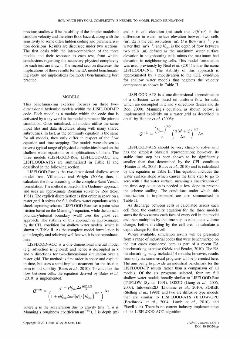
industry codes used for flood risk modelling in the UK bythe EA and commercial consultants. The industry codes(including: ISIS2D, SOBEK, TUFLOW, MIKEFLOOD,InfoWorks2D, Flowroute and JFLOW-GPU) were requiredto simulate velocity and depth dynamics across the rangetest cases listed in Table I, which were designed to cover

Table I. Summar

EA test Description

1 Flooding a disconnected water body.2 Filling of floodplain depressions.3 Momentum conservation over a smal4 Speed of flood propagation over an e5 Valley flooding following a dam fail6a and b Dam break. a) Flume scale, b) Field7 River to floodplain linking.8a and b Urban flood. a) Rainfall, b) Rainfall

Copyright © 2011 John Wiley & Sons, Ltd.

most statutory flood risk modelling requirements in the UK.In this paper, three physical process representations offloodplain flow, described in the next section, will bebenchmarked using four of the test cases from this studyidentified in Table I.One of the key issues when comparing industry codes

is the difficulty in achieving suitable consistency betweentest case implementations. Without this, there is signifi-cant uncertainty in the cause of simulation differences,meaning discrepancies between results cannot be attrib-uted to a narrow enough range of factors to allow usefulconclusions to be drawn. Differences in how modellersinterpret the same test case are the easiest to avoid byusing a single code where the state variables of each‘model’ (elevation, inflow, etc) can be taken from ashared environment. This also means model parameterswill be sourced and manipulated in a consistent manner(e.g. in the model used here, the roughness across a celledge is a linear interpolation of the roughness attributed toeach neighbouring grid cell). This degree of constancycan be assumed between models in different codes but isnot easily verified without extensive analysis of thesource code, which for commercial reasons may not beavailable. Treatment of wetting and drying, wet to dryedges, friction and source terms, inflows and normaldepth boundaries may also differ subtly between codes,both in terms of approach and parameterisation. All ofthese factors may alter simulation results before anyconsideration of numerical scheme and physical com-plexity is taken into account, adding significant uncer-tainty to any discussion.To address this issue, the models in this study were

written within a single code ensuring a level of constancybetween model state variables and parameters that was notpossible in the studies presented above. The models usedwere the full shallow water model LISFLOOD-Roe basedon the TRENT model (Villanueva and Wright, 2006), aninertial wave model LISFLOOD-ACC (Bates et al., 2010)that represents a simplified shallow water wave and adiffusion wave model LISFLOOD-ATS (Hunter et al.,2005). These all form part of the single LISFLOOD-FPcode. Results from the industry models in Néelz andPender (2010) have been used to provide context to theLISFLOOD-FP simulations, especially in regard to themagnitude of difference between the simpler and fullshallow water models. A key interest not covered by

y of test cases

Tested here

NoNo

l (0.25m) obstruction. Yesxtended floodplain. Yesure. Yes + finer resolutionscale. Yes, b only

Noand sewer surcharge. No

Hydrol. Process. (2011)DOI: 10.1002/hyp

HOW MUCH PHYSICAL COMPLEXITY IS NEEDED TO MODEL FLOOD INUNDATION?

previous studies will be the ability of the simpler models tosimulate velocity and therefore flood hazard, alongwith thesensitivity to some often hidden coding and parameterisa-tion decisions. Results are discussed under two sections.The first deals with the inter-comparison of the threemodels and their response to each test, from which,conclusions regarding the necessary physical complexityfor each test are drawn. The second section discusses theimplications of these results for the EA model benchmark-ing study and implications for model benchmarking bestpractice.

MODELS

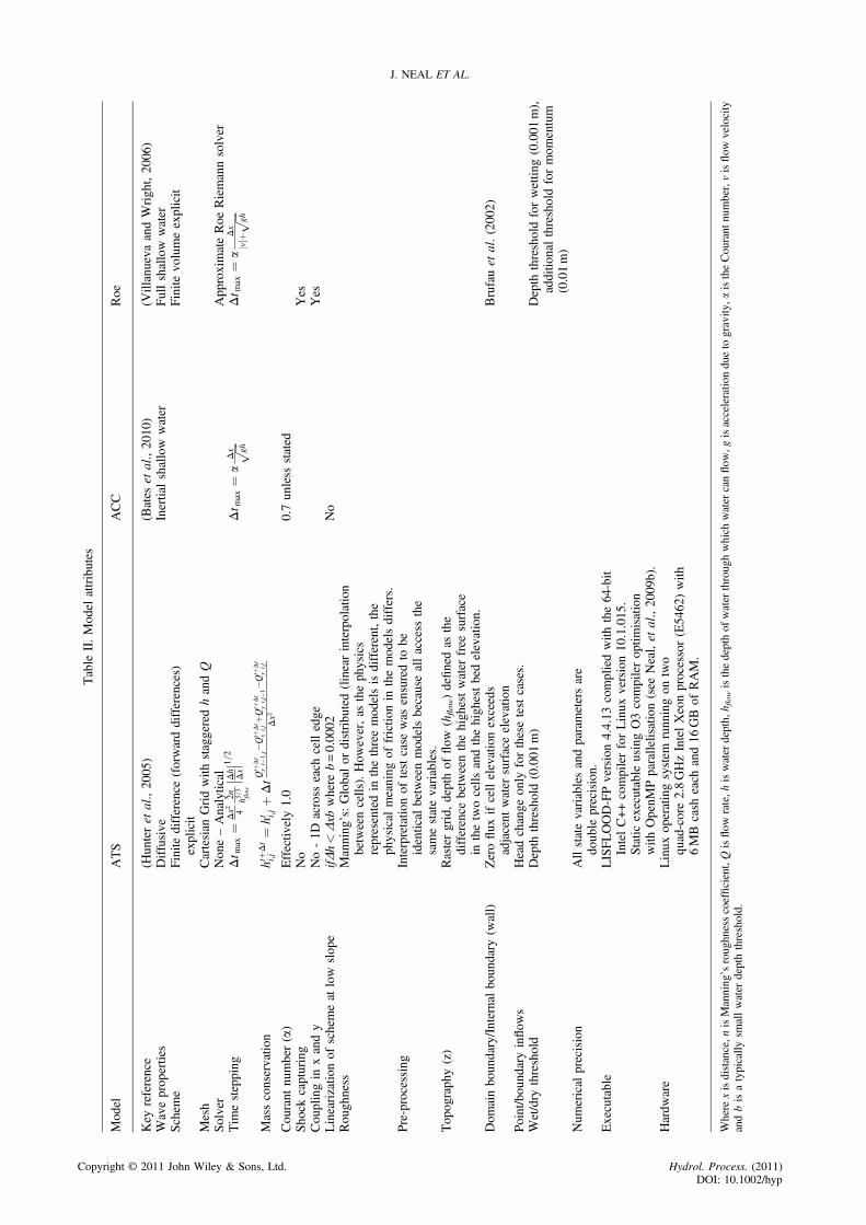
This benchmarking exercise focuses on three two-dimensional hydraulic models within the LISFLOOD-FPcode. Each model is a module within the code that isactivated by a key word in the model parameter file prior tosimulation. Once initialised, all models utilise the sameinput files and data structures, along with many sharedsubroutines. In fact, as the continuity equation is the samefor all models, they only differ in respect of the flowequation and time stepping. The models were chosen tocover a typical range of physical complexities based on theshallow water equations or simplifications of them. Thethree models (LISFLOOD-Roe, LISFLOOD-ACC andLISFLOOD-ATS) are summarised in Table II anddescribed in the following section.LISFLOOD-Roe is the two-dimensional shallow water

model from Villanueva and Wright (2006); thus, itcalculates the flow according to the complete Saint Venantformulation. Themethod is based on the Godunov approachand uses an approximate Riemann solver by Roe (Roe,1981). The explicit discretisation is first order in space on araster grid. It solves the full shallow water equations with ashock capturing scheme. LISFLOOD-Roe uses a point-wisefriction based on the Manning´s equation, while the domainboundary/internal boundary (wall) uses the ghost cellapproach. The stability of this approach is approximatedby the CFL condition for shallow water models, which isshown in Table II. As the complete model formulation isquite lengthy and relatively well known, it is not reproducedhere.LISFLOOD-ACC is a one-dimensional inertial model

(e.g. advection is ignored) and hence is decoupled in xand y directions for two-dimensional simulation over araster grid. The method is first order in space and explicitin time, but uses a semi-implicit treatment for the frictionterm to aid stability (Bates et al., 2010). To calculate theflow between cells, the equation derived by Bates et al.(2010) is implemented:

QtþΔt ¼ qt � ghtflowΔtΔ htþzð Þ

Δx

1þ ghtflowΔtn2 qtj j= htflow

� �10=3� �Δx

where g is the acceleration due to gravity (ms�1), n isManning’s roughness coefficient(sm�1/3), h is depth (m)


and z is cell elevation (m) such that Δ(ht+ z) is thedifference in water surface elevation between two cells(m), Δx is the cell resolution (m), Q is flow (m3s�1), q iswater flux (m2s�1) and htflow is the depth of flow betweentwo cells (m) defined as the maximum water surfaceelevation in neighbouring cells minus the maximum bedelevation in neighbouring cells. This model formulationwas used previously by Neal et al. (2011) under the nameLISFLOOD-INT. The stability of this approach isapproximated by a modification to the CFL conditionfor shallow water models that neglects the velocitycomponent as shown in Table II.

LISFLOOD-ATS is a one-dimensional approximationof a diffusion wave based on uniform flow formula,which are decoupled in x and y directions (Bates and deRoo, 2000). Manning’s equation, as shown below, isimplemented explicitly on a raster grid as described indetail by Hunter et al. (2005):

QtþΔt ¼htflow

� �5=3

n

Δ ht þ zð ÞΔx

� �1=2

Δx

LISFLOOD-ATS should be very cheap to solve as ithas the simplest physical representation; however, itsstable time step has been shown to be significantlysmaller than that determined by the CFL condition(Hunter et al., 2005; Bates et al., 2010) and is calculatedby the equation in Table II. This equation includes thewater surface slope which causes the time step to go tozero with a flat water surface, meaning a linearization ofthe time-step equation is needed at low slope to preventthe scheme stalling. The conditions under which thislinearization is implemented are also summarised inTable II.As discharge between cells is calculated across each

cell face, the continuity equation for the three modelssums the flows across each face of every cell in the modeland then multiplies by the time step to calculate a volumechange, before dividing by the cell area to calculate adepth change for the cell.Where available, simulation results will be presented

from a range of industrial codes that were benchmarked onthe test cases considered here as part of a recent EAbenchmarking exercise (Néelz and Pender, 2010). The EAbenchmarking study included 14 models; however, resultsfrom only six commercial programs will be presented here.The aim being to provide an industrial benchmark for theLISFLOOD-FP results rather than a comparison of allmodels. Of the six programs selected, four are fullshallow water models broadly similar to LISFLOOD-Roe(TUFLOW (Syme, 1991), ISIS2D (Liang et al., 2006,2007), Infoworks2D (Lhomme et al., 2010), SOBEK(Stelling et al., 1998)) and two are diffusive type modelsthat are similar to LISFLOOD-ATS (JFLOW-GPU(Bradbrook et al., 2004; Lamb et al., 2010) andFlowRoute). There is no current industry implementationof the LISFLOOD-ACC algorithm.


Table

II.Model

attributes

Model

ATS

ACC

Roe

Key

reference

(Hunteret

al.,2005)

(Bates

etal.,2010)

(Villanueva

andWright,2006)

Waveproperties

Diffusive

Inertialshallow

water

Fullshallow

water

Schem

eFinite

difference

(forwarddifferences)

explicit

Finite

volumeexplicit

Mesh

Cartesian

Gridwith

staggeredhandQ

Solver

None–Analytical

ApproximateRoe

Riemannsolver

Tim

estepping

Δt m

ax¼

Δx2 4

2n h5=3

flow

Δh

Δx� �� 1=2

Δt m

ax¼

aΔx ffiffiffiffi ghp

Δt m

ax¼

aΔx

v jjþ

ffiffiffiffi ghp

Massconservatio

nht

þΔt

i;j¼

ht i;jþΔtQ

tþΔt

xi�

1;j�

Qtþ

Δt

xi;jþQ

tþΔt

yi;j�

1�Q

tþΔt

yi;j

Δx2

Courant

number(a)

Effectiv

ely1.0

0.7unless

stated

Shock

capturing

No

Yes

Couplingin

xandy

No-1D

across

each

celledge

Yes

Linearizatio

nof

schemeat

low

slope

ifΔh<Δxb

where

b=0.0002

No

Roughness

Manning’s:Globalor

distributed(linearinterpolation

betweencells).How

ever,as

thephysics

representedin

thethreemodelsisdifferent,the

physical

meaning

offrictio

nin

themodelsdiffers.

Pre-processing

Interpretatio

nof

testcase

was

ensuredto

beidentical

betweenmodelsbecauseallaccess

the

samestatevariables.

Topography(z)

Rastergrid,depthof

flow

(hflow)definedas

the

difference

betweenthehighestwater

free

surface

inthetwocells

andthehighestbedelevation.

Dom

ainboundary/Internalboundary

(wall)

Zeroflux

ifcellelevationexceeds

adjacent

water

surfaceelevation

Brufauet

al.(2002)

Point/boundaryinflow

sHeadchange

only

forthesetestcases.

Wet/dry

threshold

Depth

threshold(0.001

m)

Depth

thresholdforwettin

g(0.001

m),

additio

nalthresholdformom

entum

(0.01m)

Num

erical

precision

Allstatevariablesandparametersare

double

precision.

Executable

LISFLOOD-FPversion4.4.13

compliedwith

the64-bit

IntelC++compilerforLinux

version10.1.015.

Static

executable

usingO3compileroptim

isation

with

OpenM

Pparallelisation(see

Neal,et

al.,2009b).

Hardw

are

Linux

operatingsystem

runningon

two

quad-core2.8GHzIntelXeonprocessor(E5462)with

6MBcash

each

and16

GBof

RAM.

Where

xisdistance,n

isManning’sroughnesscoefficient,Qisflow

rate,h

iswater

depth,

h flowisthedepthof

water

throughwhich

water

canflow

,gisacceleratio

ndueto

gravity

,aistheCourant

number,visflow

velocity

andbisatypically

smallwater

depththreshold.

J. NEAL ET AL.

Copyright © 2011 John Wiley & Sons, Ltd. Hydrol. Process. (2011)DOI: 10.1002/hyp


RESULTS

These results summarise findings from four of the ten EAtest cases listed in Table I. The reasons for notimplementing all tests are as follows:

• Tests 1 and 2 were ignored to save space and becauselater test were assumed to be more difficult andevaluate similar properties.

• Test 6a is a higher resolution (laboratory scale) andlower friction version of 6b. It was not practical toapply either of the simpler models to this test given theresults from test 6b.

• Tests 7, 8a and 8b were deemed outside the scope ofthis paper because they require 1D channel, rainfall andsewer models, respectively.

Before discussing the results from each test, simulationtimes are presented in Table III based on single coreimplementations of the model. Some of the simulation timedifferences between models were due to variations in theinundation dynamics between codes, particularly for testcases 3 and 6b where there was a larger variation in thenumber of wet cells. Simulated dynamics were more alikein tests 4 and 5 (see subsequent results sections) meaningthe difference in simulation time between the modelsprovides indicative data on their relative speeds. For test 4,which has the longest simulation time, LISFLOOD-Roewas 3.3 times slower than LISFLOOD-ACC and 116.2times faster than LISFLOOD-ATS. These differences werenot unexpected. For LISFLOOD-ATS, the time step isproportional to Δx2 rather than Δx as is the case with theother models, whilst the inclusion of potentially very smallwater surface slopes in the time-stepping equation (seeTable II) will further reduce the time step relative to theother codes, especially if the computational grid is alignedwith the water surface contours. Unlike LISFLOOD-ACC,LISFLOOD-Roe includes absolute velocity in the time-stepping equation because advection is included in themodel physics. Another indicator of potential computa-tional efficiency is the relative number of non-integerpower functions needed to calculate flow in each model,these are nine (LISFLOOD-Roe), one (LISFLOOD-ACC)and two (LISFLOOD-ATS). Thus, LISFLOOD-ACCrequires a similar amount of computation per time step toLISFLOOD-ATS and significantly less computation per

Table III. Summary of test c

Test 3 Test 4 Test

Simulationtime

Number oftime steps

Simulationtime

Number oftime steps

Simulatiotime

Roe 0.07 905 6.48 15291 2.55**ACC 0.03 900 1.97 10551 0.68ATS 1.52 82835 228.95 654581 161.13

*cfl number reduced to 0.5 for stability.**cfl number reduced to 0.3 for stability.+ run on two CPU cores.++ run on eight CPU cores.


time step than LISFLOOD-Roe. The relative simulationtimes vary between the test cases due to resolution,velocity, depth and slope factors, although in all but onecase, the rank order of the models in terms of simulationtime was consistent. Note that all three LISFLOOD-FPmodels are explicit in time and that implicit schemes wouldallow longer time steps to be used.Mass balance errors for each model simulation are

summarised in Table IV using the cumulative volumeerror (m3) at the end of each simulation, which is the sumof volume errors made by the model calculated at regularintervals through the simulation. Such that:

Ve ¼ VN � VO þXNi¼1

ΔtiQiin �

XNi¼1

ΔtiQiout

where the volume error Ve over a period of N time steps isthe initial domain volume V0 plus the sum of inflowvolumes ΔtQin over each of the N time steps minus thesum of outflow volumes from the domain ΔtQout minusthe domain volume at the end of the N time steps VN. Asall the test cases used here have closed boundaries at theedge of the domain, the outflow volumes were zero.LISFLOOD-ATS tended to have the smallest volumeerrors, and these were always several orders of magnitudebelow 1% of the domain volume. LISFLOOD-ACCeither had the smallest or greatest mass error dependingon the test case. Reasons for larger mass errors inLISFLOOD-ACC simulations of test case 3 and 6b andLISFLOOD-Roe simulations of tests 4 and 5 arediscussed in subsequent test case specific sections.

Momentum conservation over a bump

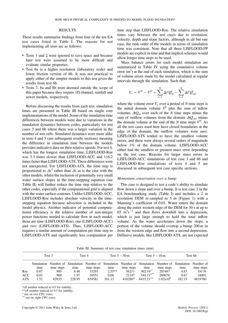
This case is designed to test a code’s ability to simulateflow down a slope and over a bump. It is test case 3 in theEA benchmarking study (Table I) and includes a 2 mresolution DEM re-sampled to 5 m (Figure 1) with aManning’s coefficient of 0.01. Water enters the domainalong the entire western edge of the DEM for 30 s at up to65 m3s�1 and then flows downhill into a depression,which is just large enough to hold the total inflowvolume. As the water accelerates down the slope, aportion of the volume should overtop a bump 200m infrom the western edge and flow into a second depression.Diffusive models, like LISFLOOD-ATS, are not expected

ase simulation times (min)

5 – 50m Test 5 – 10m Test 6b

n Number oftime steps

Simulationtime

Number oftime steps

Simulationtime

Number oftime steps

56211 302.19+* 207487 4.67 1817621147 344.11+** 260676 0.67 18001

4102887 6415.21++ 1.02x108 182.15 4819760


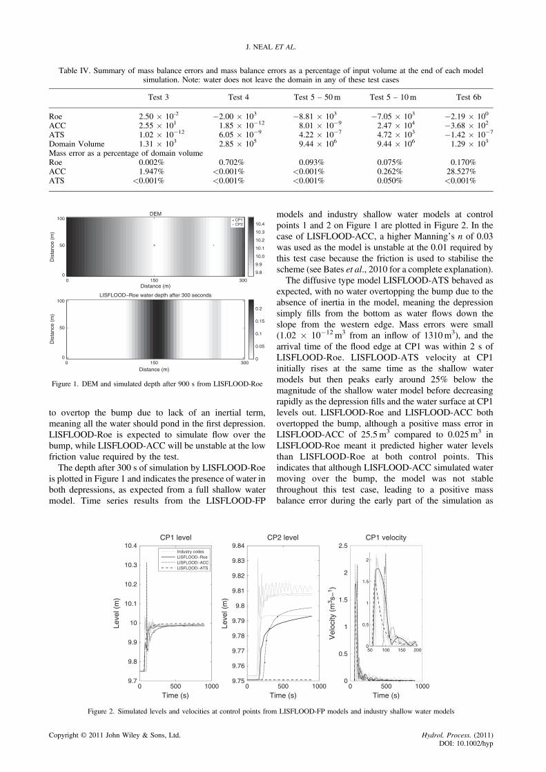
Table IV. Summary of mass balance errors and mass balance errors as a percentage of input volume at the end of each modelsimulation. Note: water does not leave the domain in any of these test cases

Test 3 Test 4 Test 5 – 50m Test 5 – 10m Test 6b

Roe 2.50 � 10-2 �2.00 � 103 �8.81 � 103 �7.05 � 103 �2.19 � 100

ACC 2.55 � 101 1.85 � 10�12 8.01 � 10�9 2.47 � 104 �3.68 � 102

ATS 1.02 � 10�12 6.05 � 10�9 4.22 � 10�7 4.72 � 103 �1.42 � 10�7

Domain Volume 1.31 � 103 2.85 � 105 9.44 � 106 9.44 � 106 1.29 � 103

Mass error as a percentage of domain volumeRoe 0.002% 0.702% 0.093% 0.075% 0.170%ACC 1.947% <0.001% <0.001% 0.262% 28.527%ATS <0.001% <0.001% <0.001% 0.050% <0.001%

DEM

0 150 300

100

50

0

100

50

0

LISFLOOD−Roe water depth after 300 seconds

0 150 300

9.8

9.9

10.0

10.1

10.2

10.3

10.4

0

0.05

0.1

0.15

0.2

Distance (m)

Distance (m)

Dis

tanc

e (m

)D

ista

nce

(m)

CP1CP2

Figure 1. DEM and simulated depth after 900 s from LISFLOOD-Roe

J. NEAL ET AL.

to overtop the bump due to lack of an inertial term,meaning all the water should pond in the first depression.LISFLOOD-Roe is expected to simulate flow over thebump, while LISFLOOD-ACC will be unstable at the lowfriction value required by the test.The depth after 300 s of simulation by LISFLOOD-Roe

is plotted in Figure 1 and indicates the presence of water inboth depressions, as expected from a full shallow watermodel. Time series results from the LISFLOOD-FP

0 500 10009.7

9.8

9.9

10

10.1

10.2

10.3

10.4CP1 level CP

Time (s)

Leve

l (m

)

09.75

9.76

9.77

9.78

9.79

9.8

9.81

9.82

9.83

9.84

T

Leve

l (m

)

Industry codesLISFLOOD−RoeLISFLOOD−ACCLISFLOOD−ATS

Figure 2. Simulated levels and velocities at control points from


models and industry shallow water models at controlpoints 1 and 2 on Figure 1 are plotted in Figure 2. In thecase of LISFLOOD-ACC, a higher Manning’s n of 0.03was used as the model is unstable at the 0.01 required bythis test case because the friction is used to stabilise thescheme (see Bates et al., 2010 for a complete explanation).The diffusive type model LISFLOOD-ATS behaved as

expected, with no water overtopping the bump due to theabsence of inertia in the model, meaning the depressionsimply fills from the bottom as water flows down theslope from the western edge. Mass errors were small(1.02 � 10�12m3 from an inflow of 1310m3), and thearrival time of the flood edge at CP1 was within 2 s ofLISFLOOD-Roe. LISFLOOD-ATS velocity at CP1initially rises at the same time as the shallow watermodels but then peaks early around 25% below themagnitude of the shallow water model before decreasingrapidly as the depression fills and the water surface at CP1levels out. LISFLOOD-Roe and LISFLOOD-ACC bothovertopped the bump, although a positive mass error inLISFLOOD-ACC of 25.5m3 compared to 0.025m3 inLISFLOOD-Roe meant it predicted higher water levelsthan LISFLOOD-Roe at both control points. Thisindicates that although LISFLOOD-ACC simulated watermoving over the bump, the model was not stablethroughout this test case, leading to a positive massbalance error during the early part of the simulation as

CP1 velocity2 level

500 1000

ime (s)0 500 1000

0

0.5

1

1.5

2

2.5

Time (s)

Vel

ocity

(m

3 s−

1 )

50 100 150 2000

0.5

1

1.5

2

LISFLOOD-FP models and industry shallow water models


0 50 100 150 200 250 300 350 4000

5

10

15

20

25

Time (minutes)

Inflow

Inflo

w (

m3 s

−1 )

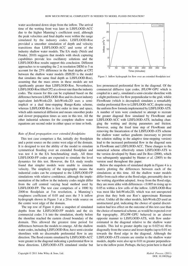
Figure 3. Inflow hydrograph for flow over an extended floodplain test


water accelerated down slope from the inflow. The arrivaltime of the wetting front was later in LISFLOOD-ACCdue to the higher Manning’s coefficient used, althoughthe peak velocities and final depths were within the rangesimulated by the industry codes. LISFLOOD-Roeprovided a smoother simulation of depth and velocitytransitions than LISFLOOD-ACC and some of theindustry shallow water models. The EA study (Néelz andPender, 2010) suggests that models with shock capturingcapabilities provide less oscillatory solutions and theLISFLOOD-Roe results support this conclusion. Differentapproaches to re-sampling the 2 m resolution DEM to 5 maccount for the 25% difference in the final depths at CP2between the shallow water models (ISIS2D is the modelthat simulates the same final depth as LISFLOOD-Roe),assuming that the mass errors in these models are notsignificantly greater than LISFLOOD-Roe. Nevertheless,LISFLOOD-Roe filled CP2 at a slower rate than the industrycodes. The reason for this can be explained based on thedifference between LISFLOOD-Roe and its closest industryequivalent InfoWorks2D. InfoWorks2D uses a semi-implicit or a dual time-stepping Runge-Kutta scheme,whereas LISFLOOD-Roe is first order in time and space,which adds numerical diffusion and means smoother peaksand slower propagation times as seen in this test. All theother industrial schemes for the complete shallow waterequations are second order in either space or time or both.

Rate of flood propagation over extended floodplains

This test case comprises a flat, initially dry floodplainand a point source on the centre west edge of the domain.It is designed to test the ability of the model to simulatesymmetrical flooding over an extended floodplain andwas test 4 in the EA benchmarking study. All threeLISFLOOD-FP codes are expected to simulate the leveldynamics for this test. However, the EA study resultsfound that simpler models were unable to simulatevelocity. The simplicity of the topography means theindustrial codes can be compared to the LISFLOOD-FPsimulations with relative confidence, although the imple-mentation of the inflow in the industry codes might differfrom the cell centred varying head method used byLISFLOOD-FP. The test case comprises of a 1000 by2000 m floodplain at 5 m resolution, a Manning’sroughness coefficient of 0.05 and uses the 5 h inflowhydrograph shown in Figure 3 at a 20m wide source onthe centre west edge of the domain.The top row of Figure 4 plots a snapshot of simulated

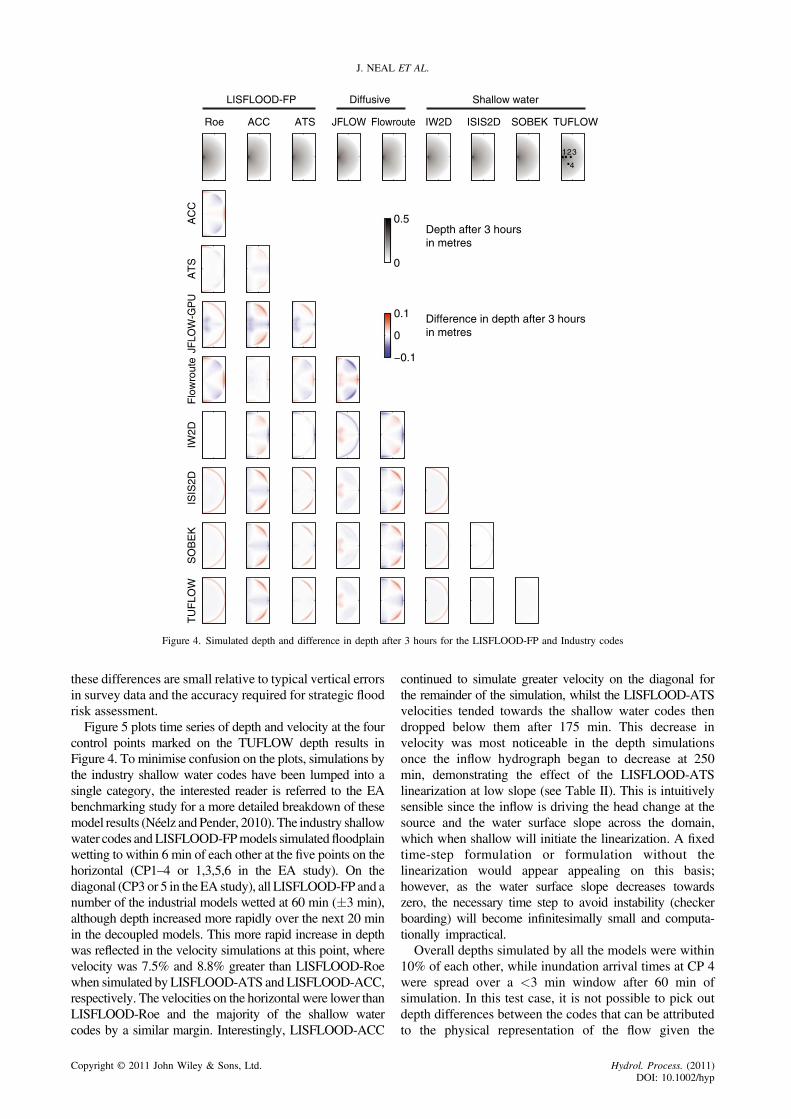
depths from the LISFLOOD-FP models and the sixcommercial codes 3 h into the simulation, shortly beforethe shoreline reached the eastern closed boundary of thedomain. This allowed the greatest time period fordifferences between the models to emerge. All the shallowwater codes, including LISFLOOD-Roe, have semi-circularshorelines with no discernable preferential flow in anydirection. The flood extents simulated by LISFLOOD-ACCwere greater in the diagonal indicating a preferential flow inthese directions. LISFLOOD-ATS simulated similar but


less pronounced preferential flow in the diagonal. Of thecommercial diffusive type codes, JFLOW-GPU which iscoupled in x and y, simulated a semi-circular shoreline witha slight preference for flow perpendicular to the grid, whilstFlowRoute (which is decoupled) simulates a remarkablysimilar preferential flow to LISFLOOD-ACC, despite usingthe uniform flow formula implemented by LISFLOOD-ATS.A number of tests were conducted to attempt to recreatethe greater diagonal flow simulated by FlowRoute andLISFLOOD-ACC with LISFLOOD-ATS, including chan-ging the wetting and drying parameters and friction.However, using the fixed time step of FlowRoute andremoving the linearization of the LISFLOOD-ATS schemefor shallow water surface gradients (necessary to preventthe solution stalling in the adaptive time-stepping version)lead to the increased preferential flow in the diagonal seenin FlowRoute and LISFLOOD-ACC. These changes to thenumerical scheme effectively return LISFLOOD-ATS tothe version developed by Bates and De Roo (2000), whichwas subsequently upgraded by Hunter et al. (2005) to theversion used throughout this paper.Below the snapshots of simulated depth in Figure 4 is a

matrix plotting the differences between each of thesimulations at this time. All the shallow water modelsdiffer from each other at the flood edge, presumably due tothe wetting algorithm adopted. Away from the flood edge,they are more alike with differences <0.005m rising up to0.05m within a few cells of the inflow. LISFLOOD-Roewas most like InfoWorks2D, which was not unexpectedgiven that they both use Roe’s approximate Riemannsolver. Unlike all the other models, InfoWorks2D used anunstructured grid, indicating the choice of spatial discret-isation had less effect on the outcome of this test case thanthe choice of numerical scheme, as would be expected overflat topography. JFLOW-GPU behaved in an almostopposite manner to LISFLOOD-ATS, with flow under-estimated in the diagonal relative to the shallow watermodels. This led to greater depths (up to 0.025m) 40mdiagonally from the source and lesser depths (up to 0.01m)towards the flood edge in the diagonal. Although theLISFLOOD-ATS extents are similar to the shallow watermodels, depths were also up to 0.01m greater perpendicu-lar to the inflow point. Perhaps, the key point here is that all


Roe

Shallow waterDiffusiveLISFLOOD-FP

ACC ATS JFLOW Flowroute IW2D ISIS2D SOBEK TUFLOW

AT

SA

CC

JFLO

W-G

PU

Flo

wro

ute

IW2D

ISIS

2DS

OB

EK

TU

FLO

W

0

0.5

−0.1

0

0.1 Difference in depth after 3 hoursin metres

Depth after 3 hoursin metres

1 2 3

4

Figure 4. Simulated depth and difference in depth after 3 hours for the LISFLOOD-FP and Industry codes

J. NEAL ET AL.

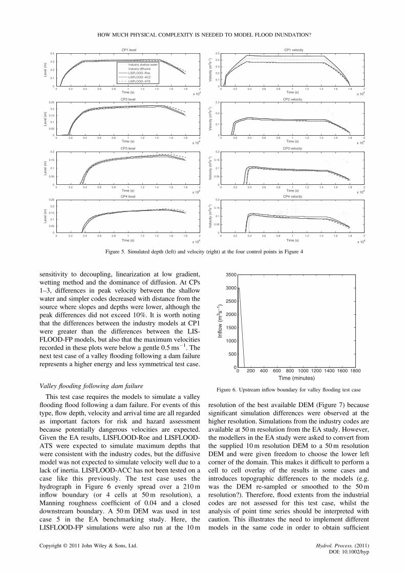
these differences are small relative to typical vertical errorsin survey data and the accuracy required for strategic floodrisk assessment.Figure 5 plots time series of depth and velocity at the four

control points marked on the TUFLOW depth results inFigure 4. To minimise confusion on the plots, simulations bythe industry shallow water codes have been lumped into asingle category, the interested reader is referred to the EAbenchmarking study for a more detailed breakdown of thesemodel results (Néelz andPender, 2010). The industry shallowwater codes andLISFLOOD-FPmodels simulatedfloodplainwetting to within 6 min of each other at the five points on thehorizontal (CP1–4 or 1,3,5,6 in the EA study). On thediagonal (CP3 or 5 in the EA study), all LISFLOOD-FP and anumber of the industrial models wetted at 60 min (�3 min),although depth increased more rapidly over the next 20 minin the decoupled models. This more rapid increase in depthwas reflected in the velocity simulations at this point, wherevelocity was 7.5% and 8.8% greater than LISFLOOD-Roewhen simulated by LISFLOOD-ATS and LISFLOOD-ACC,respectively. The velocities on the horizontal were lower thanLISFLOOD-Roe and the majority of the shallow watercodes by a similar margin. Interestingly, LISFLOOD-ACC


continued to simulate greater velocity on the diagonal forthe remainder of the simulation, whilst the LISFLOOD-ATSvelocities tended towards the shallow water codes thendropped below them after 175 min. This decrease invelocity was most noticeable in the depth simulationsonce the inflow hydrograph began to decrease at 250min, demonstrating the effect of the LISFLOOD-ATSlinearization at low slope (see Table II). This is intuitivelysensible since the inflow is driving the head change at thesource and the water surface slope across the domain,which when shallow will initiate the linearization. A fixedtime-step formulation or formulation without thelinearization would appear appealing on this basis;however, as the water surface slope decreases towardszero, the necessary time step to avoid instability (checkerboarding) will become infinitesimally small and computa-tionally impractical.Overall depths simulated by all the models were within

10% of each other, while inundation arrival times at CP 4were spread over a <3 min window after 60 min ofsimulation. In this test case, it is not possible to pick outdepth differences between the codes that can be attributedto the physical representation of the flow given the


0 0.2 0.4 0.6 0.8 1 1.2 1.4 1.6 1.8 2

x 104

0

0.1

0.2

0.3

0.4

Time (s)

Leve

l (m

)

CP1 level

Industry shallow waterIndustry diffusiveLISFLOOD−RoeLISFLOOD−ACCLISFLOOD−ATS

0 0.2 0.4 0.6 0.8 1 1.2 1.4 1.6 1.8 2

x 104

0

0.05

0.1

0.15

0.2

0.25

Time (s)

Leve

l (m

)

CP2 level

0 0.2 0.4 0.6 0.8 1 1.2 1.4 1.6 1.8 2

x 104

0

0.05

0.1

0.15

0.2

Time (s)

Leve

l (m

)

CP3 level

0 0.2 0.4 0.6 0.8 1 1.2 1.4 1.6 1.8 2

x 104

0

0.05

0.1

0.15

0.2

0.25

Time (s)

Leve

l (m

)

CP4 level

0 0.2 0.4 0.6 0.8 1 1.2 1.4 1.6 1.8 2

x 104

0

0.1

0.2

0.3

0.4

0.5

Time (s)

Vel

ocity

(m

3 s-1

)V

eloc

ity (

m3 s

-1)

CP1 velocity

0 0.2 0.4 0.6 0.8 1 1.2 1.4 1.6 1.8 20

0.1

0.2

0.3

Time (s)

CP2 velocity

0 0.2 0.4 0.6 0.8 1 1.2 1.4 1.6 1.8 20

0.05

0.1

0.15

0.2

Time (s)

CP3 velocity

0 0.2 0.4 0.6 0.8 1 1.2 1.4 1.6 1.8 20

0.05

0.1

0.15

0.2

Time (s)

CP4 velocity

Vel

ocity

(m

3 s-1

)V

eloc

ity (

m3 s

-1)

x 104

x 104

x 104

Figure 5. Simulated depth (left) and velocity (right) at the four control points in Figure 4

0

500

1000

1500

2000

2500

3000

3500

Inflo

w (

m3 s

−1 )


sensitivity to decoupling, linearization at low gradient,wetting method and the dominance of diffusion. At CPs1–3, differences in peak velocity between the shallowwater and simpler codes decreased with distance from thesource where slopes and depths were lower, although thepeak differences did not exceed 10%. It is worth notingthat the differences between the industry models at CP1were greater than the differences between the LIS-FLOOD-FP models, but also that the maximum velocitiesrecorded in these plots were below a gentle 0.5ms�1. Thenext test case of a valley flooding following a dam failurerepresents a higher energy and less symmetrical test case.

0 200 400 600 800 1000 1200 1400 1600 1800

Time (minutes)

Figure 6. Upstream inflow boundary for valley flooding test case
Valley flooding following dam failure
This test case requires the models to simulate a valleyflooding flood following a dam failure. For events of thistype, flow depth, velocity and arrival time are all regardedas important factors for risk and hazard assessmentbecause potentially dangerous velocities are expected.Given the EA results, LISFLOOD-Roe and LISFLOOD-ATS were expected to simulate maximum depths thatwere consistent with the industry codes, but the diffusivemodel was not expected to simulate velocity well due to alack of inertia. LISFLOOD-ACC has not been tested on acase like this previously. The test case uses thehydrograph in Figure 6 evenly spread over a 210minflow boundary (or 4 cells at 50m resolution), aManning roughness coefficient of 0.04 and a closeddownstream boundary. A 50m DEM was used in testcase 5 in the EA benchmarking study. Here, theLISFLOOD-FP simulations were also run at the 10m


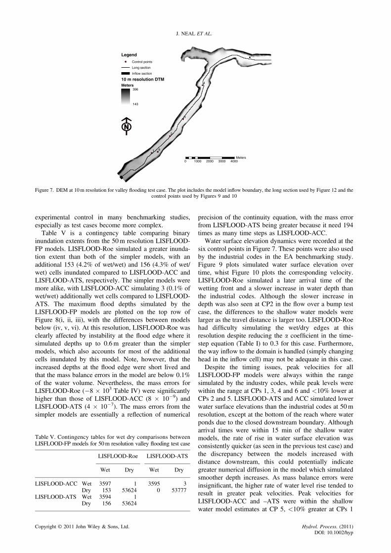
resolution of the best available DEM (Figure 7) becausesignificant simulation differences were observed at thehigher resolution. Simulations from the industry codes areavailable at 50m resolution from the EA study. However,the modellers in the EA study were asked to convert fromthe supplied 10m resolution DEM to a 50m resolutionDEM and were given freedom to choose the lower leftcorner of the domain. This makes it difficult to perform acell to cell overlay of the results in some cases andintroduces topographic differences to the models (e.g.was the DEM re-sampled or smoothed to the 50mresolution?). Therefore, flood extents from the industrialcodes are not assessed for this test case, whilst theanalysis of point time series should be interpreted withcaution. This illustrates the need to implement differentmodels in the same code in order to obtain sufficient


6

5

4

3

2

1

Legend

Control points

Long section

Inflow section

10 m resolution DTMMeters

1000 2000 30000 4000Meters

396

143

Figure 7. DEM at 10m resolution for valley flooding test case. The plot includes the model inflow boundary, the long section used by Figure 12 and thecontrol points used by Figures 9 and 10

J. NEAL ET AL.

experimental control in many benchmarking studies,especially as test cases become more complex.Table V is a contingency table comparing binary

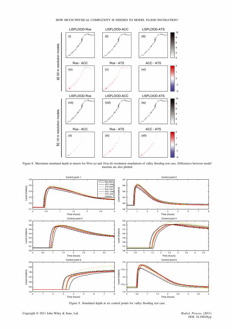
inundation extents from the 50m resolution LISFLOOD-FP models. LISFLOOD-Roe simulated a greater inunda-tion extent than both of the simpler models, with anadditional 153 (4.2% of wet/wet) and 156 (4.3% of wet/wet) cells inundated compared to LISFLOOD-ACC andLISFLOOD-ATS, respectively. The simpler models weremore alike, with LISFLOOD-ACC simulating 3 (0.1% ofwet/wet) additionally wet cells compared to LISFLOOD-ATS. The maximum flood depths simulated by theLISFLOOD-FP models are plotted on the top row ofFigure 8(i, ii, iii), with the differences between modelsbelow (iv, v, vi). At this resolution, LISFLOOD-Roe wasclearly affected by instability at the flood edge where itsimulated depths up to 0.6m greater than the simplermodels, which also accounts for most of the additionalcells inundated by this model. Note, however, that theincreased depths at the flood edge were short lived andthat the mass balance errors in the model are below 0.1%of the water volume. Nevertheless, the mass errors forLISFLOOD-Roe (�8 � 103 Table IV) were significantlyhigher than those of LISFLOOD-ACC (8 � 10�9) andLISFLOOD-ATS (4 � 10�7). The mass errors from thesimpler models are essentially a reflection of numerical

Table V. Contingency tables for wet dry comparisons betweenLISFLOOD-FP models for 50m resolution valley flooding test case

LISFLOOD-Roe LISFLOOD-ATS

Wet Dry Wet Dry

LISFLOOD-ACC Wet 3597 1 3595 3Dry 153 53624 0 53777

LISFLOOD-ATS Wet 3594 1Dry 156 53624


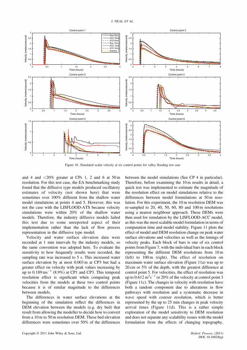
precision of the continuity equation, with the mass errorfrom LISFLOOD-ATS being greater because it need 194times as many time steps as LISFLOOD-ACC.Water surface elevation dynamics were recorded at the

six control points in Figure 7. These points were also usedby the industrial codes in the EA benchmarking study.Figure 9 plots simulated water surface elevation overtime, whist Figure 10 plots the corresponding velocity.LISFLOOD-Roe simulated a later arrival time of thewetting front and a slower increase in water depth thanthe industrial codes. Although the slower increase indepth was also seen at CP2 in the flow over a bump testcase, the differences to the shallow water models werelarger as the travel distance is larger too. LISFLOOD-Roehad difficulty simulating the wet/dry edges at thisresolution despite reducing the a coefficient in the time-step equation (Table I) to 0.3 for this case. Furthermore,the way inflow to the domain is handled (simply changinghead in the inflow cell) may not be adequate in this case.Despite the timing issues, peak velocities for all

LISFLOOD-FP models were always within the rangesimulated by the industry codes, while peak levels werewithin the range at CPs 1, 3, 4 and 6 and <10% lower atCPs 2 and 5. LISFLOOD-ATS and ACC simulated lowerwater surface elevations than the industrial codes at 50mresolution, except at the bottom of the reach where waterponds due to the closed downstream boundary. Althougharrival times were within 15 min of the shallow watermodels, the rate of rise in water surface elevation wasconsistently quicker (as seen in the previous test case) andthe discrepancy between the models increased withdistance downstream, this could potentially indicategreater numerical diffusion in the model which simulatedsmoother depth increases. As mass balance errors wereinsignificant, the higher rate of water level rise tended toresult in greater peak velocities. Peak velocities forLISFLOOD-ACC and –ATS were within the shallowwater model estimates at CP 5, <10% greater at CPs 1


−2

−1

0

1

2

0

2

4

6

8

10

−2

−1

0

1

2

LISFLOOD-Roe

LISFLOOD-ACC

LISFLOOD-ATS

0

2

4

6

8

10

b) 1

0 m

res

olut

ion

mod

els

a) 5

0 m

res

olut

ion

mod

els

Roe - ACC Roe - ATS ACC - ATS

Roe - ACC Roe - ATS ACC - ATS

LISFLOOD-Roe LISFLOOD-ACC LISFLOOD-ATS

(v) (vi)(iv)

(ii) (iii)(i)

(viii) (ix)(vii)

(xi) (xii)(x)

Figure 8. Maximum simulated depth in meters for 50m (a) and 10m (b) resolution simulations of valley flooding test case. Differences between modelmaxima are also plotted

0 0.5 1 1.5 2 2.5 3171

172

173

174

175

176Control point 1

Time (hours)

Leve

l (m

eter

s)

0 1 2 3 4 5 6 7 8162

163

164

165

166

167Control point 2

Time (hours)

Leve

l (m

eter

s)

0 0.5 1 1.5 2 2.5 3 3.5 4150

151

152

153

154

155

156

157Control point 3

Time (hours)

Leve

l (m

eter

s)

0 0.5 1 1.5 2 2.5 3 3.5 4 4.5146

147

148

149

150

151

152

153Control point 4

Time (hours)

Leve

l (m

eter

s)

0 1 2 3 4 5 6 7 8144

145

146

147

148

149

150Control point 5

Time (hours)

Leve

l (m

eter

s)

0 0.5 1 1.5 2 2.5 3 3.5 4172

172.5

173

173.5

174Control point 6

Time (hours)

Leve

l (m

eter

s)

Roe 50mACC 50mATS 50mRoe 10mACC 10mATS 10mIndustry

Figure 9. Simulated depth at six control points for valley flooding test case


Copyright © 2011 John Wiley & Sons, Ltd. Hydrol. Process. (2011)DOI: 10.1002/hyp

0 0.5 1 1.5 2 2.5 30

0.5

1

1.5

2

2.5

3Control point 1

Time (hours)

Vel

ocity

(m

eter

s/se

cond

)

0 1 2 3 4 5 6 7 80

0.5

1

1.5

2

2.5

3Control point 2

Time (hours)

Vel

ocity

(m

eter

s/se

cond

)

0 0.5 1 1.5 2 2.5 3 3.5 40

0.5

1

1.5

2

2.5Control point 3

Time (hours)

Vel

ocity

(m

eter

s/se

cond

)

0 0.5 1 1.5 2 2.5 3 3.5 4 4.50

0.5

1

1.5

2

2.5Control point 4

Time (hours)

Vel

ocity

(m

eter

s/se

cond

)

0 1 2 3 4 5 6 7 80

0.5

1

1.5Control point 5

Time (hours)

Vel

ocity

(m

eter

s/se

cond

)

0 0.5 1 1.5 2 2.5 3 3.5 40

0.5

1

1.5

2

2.5

3

3.5Control point 6

Time (hours)

Vel

ocity

(m

eter

s/se

cond

)

Roe 50mACC 50mATS 50mRoe 10mACC 10mATS 10mIndustry

Figure 10. Simulated scalar velocity at six control points for valley flooding test case

J. NEAL ET AL.

and 4 and <20% greater at CPs 1, 2 and 6 at 50mresolution. For this test case, the EA benchmarking studyfound that the diffusive type models produced oscillatoryestimates of velocity (not shown here) that weresometimes over 100% different from the shallow watermodel simulations at points 4 and 5. However, this wasnot the case with the LISFLOOD-ATS because velocitysimulations were within 20% of the shallow watermodels. Therefore, the industry diffusive models failedthis test due to some unreported aspect of theirimplementation rather than the lack of flow processrepresentation in the diffusive type model.Velocity and water surface elevation data were

recorded at 1 min intervals by the industry models, sothe same convention was adopted here. To evaluate thesensitivity to how frequently results were recorded, thesampling rate was increased to 5 s. This increased watersurface elevation by at most 0.003m at CP3 but had agreater effect on velocity with peak values increasing byup to 0.189ms�1 (8.9%) at CP1 and CP3. This temporalresolution effect is significant when comparing peakvelocities from the models at these two control pointsbecause it is of similar magnitude to the differencesbetween models.The differences in water surface elevations at the

beginning of the simulation reflect the differences inDEM elevation between the models (e.g. dry bed) thatresult from allowing the modeller to decide how to convertfrom a 10m to 50m resolution DEM. These bed elevationdifferences were sometimes over 50% of the differences


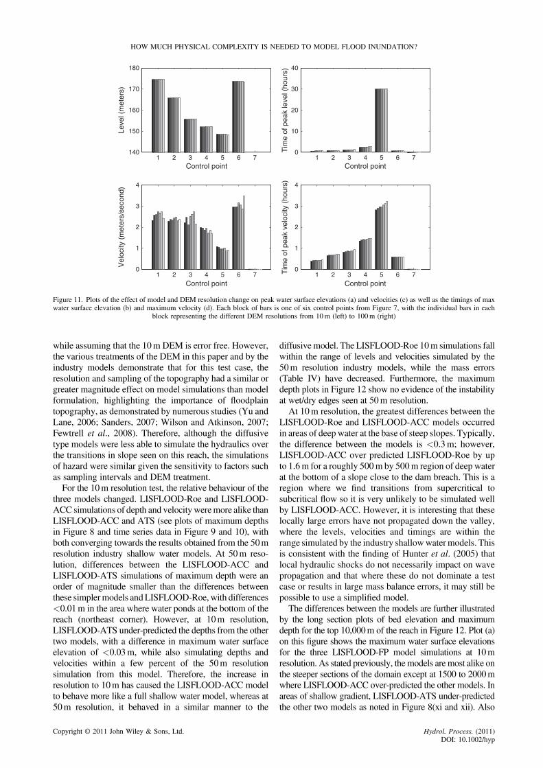
between the model simulations (See CP 4 in particular).Therefore, before examining the 10m results in detail, aquick test was implemented to estimate the magnitude ofthe resolution effect on model simulations relative to thedifferences between model formulations at 50m reso-lution. For this experiment, the 10m resolution DEM wasre-sampled to 20, 40, 50, 60, 80 and 100m resolutionsusing a nearest neighbour approach. These DEMs werethen used for simulation by the LISFLOOD-ACC model,as this was the most scalable model formulation in terms ofcomputation time and model stability. Figure 11 plots theeffect of model and DEM resolution change on peak watersurface elevations and velocities as well as the timings ofvelocity peaks. Each block of bars is one of six controlpoints from Figure 7, with the individual bars in each blockrepresenting the different DEM resolutions from 10m(left) to 100m (right). The effect of resolution onmaximum water surface elevation (Figure 11a) was up to20 cm or 5% of the depth, with the greatest difference atcontrol point 5. For velocities, the effect of resolution wasup to 0.612 m3s�1 or 20% of the velocity at control point 3(Figure 11c). The changes in velocity with resolution haveboth a random component due to alterations in flowpathways with resolution and a systematic decrease inwave speed with courser resolution, which is betterrepresented by the up to 25 min changes in peak velocityarrival times (Figure 11d). This is a rather simpleexploration of the model sensitivity to DEM resolutionand does not separate any scalability issues with the modelformulation from the effects of changing topography,


1 2 3 4 5 6 7140

150

160

170

180

Control point

Leve

l (m

eter

s)

1 2 3 4 5 6 70

10

20

30

40

Control point

Tim

e of

pea

k le

vel (

hour

s)1 2 3 4 5 6 7

0

1

2

3

4

Control point

Vel

ocity

(m

eter

s/se

cond

)

1 2 3 4 5 6 70

1

2

3

4

Control pointT

ime

of p

eak

velo

city

(ho

urs)

Figure 11. Plots of the effect of model and DEM resolution change on peak water surface elevations (a) and velocities (c) as well as the timings of maxwater surface elevation (b) and maximum velocity (d). Each block of bars is one of six control points from Figure 7, with the individual bars in each

block representing the different DEM resolutions from 10m (left) to 100m (right)


while assuming that the 10m DEM is error free. However,the various treatments of the DEM in this paper and by theindustry models demonstrate that for this test case, theresolution and sampling of the topography had a similar orgreater magnitude effect on model simulations than modelformulation, highlighting the importance of floodplaintopography, as demonstrated by numerous studies (Yu andLane, 2006; Sanders, 2007; Wilson and Atkinson, 2007;Fewtrell et al., 2008). Therefore, although the diffusivetype models were less able to simulate the hydraulics overthe transitions in slope seen on this reach, the simulationsof hazard were similar given the sensitivity to factors suchas sampling intervals and DEM treatment.For the 10m resolution test, the relative behaviour of the

three models changed. LISFLOOD-Roe and LISFLOOD-ACC simulations of depth and velocity weremore alike thanLISFLOOD-ACC and ATS (see plots of maximum depthsin Figure 8 and time series data in Figure 9 and 10), withboth converging towards the results obtained from the 50mresolution industry shallow water models. At 50m reso-lution, differences between the LISFLOOD-ACC andLISFLOOD-ATS simulations of maximum depth were anorder of magnitude smaller than the differences betweenthese simplermodels andLISFLOOD-Roe, with differences<0.01m in the area where water ponds at the bottom of thereach (northeast corner). However, at 10m resolution,LISFLOOD-ATS under-predicted the depths from the othertwo models, with a difference in maximum water surfaceelevation of <0.03m, while also simulating depths andvelocities within a few percent of the 50m resolutionsimulation from this model. Therefore, the increase inresolution to 10m has caused the LISFLOOD-ACC modelto behave more like a full shallow water model, whereas at50m resolution, it behaved in a similar manner to the


diffusive model. The LISFLOOD-Roe 10m simulations fallwithin the range of levels and velocities simulated by the50m resolution industry models, while the mass errors(Table IV) have decreased. Furthermore, the maximumdepth plots in Figure 12 show no evidence of the instabilityat wet/dry edges seen at 50m resolution.At 10m resolution, the greatest differences between the

LISFLOOD-Roe and LISFLOOD-ACC models occurredin areas of deep water at the base of steep slopes. Typically,the difference between the models is <0.3m; however,LISFLOOD-ACC over predicted LISFLOOD-Roe by upto 1.6m for a roughly 500m by 500m region of deep waterat the bottom of a slope close to the dam breach. This is aregion where we find transitions from supercritical tosubcritical flow so it is very unlikely to be simulated wellby LISFLOOD-ACC. However, it is interesting that theselocally large errors have not propagated down the valley,where the levels, velocities and timings are within therange simulated by the industry shallowwater models. Thisis consistent with the finding of Hunter et al. (2005) thatlocal hydraulic shocks do not necessarily impact on wavepropagation and that where these do not dominate a testcase or results in large mass balance errors, it may still bepossible to use a simplified model.The differences between the models are further illustrated

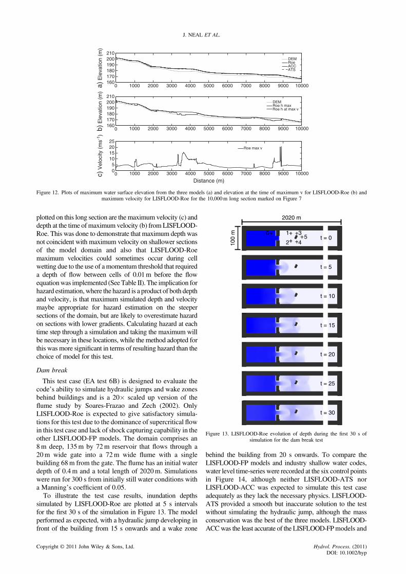
by the long section plots of bed elevation and maximumdepth for the top 10,000m of the reach in Figure 12. Plot (a)on this figure shows the maximum water surface elevationsfor the three LISFLOOD-FP model simulations at 10mresolution. As stated previously, the models are most alike onthe steeper sections of the domain except at 1500 to 2000mwhere LISFLOOD-ACC over-predicted the other models. Inareas of shallow gradient, LISFLOOD-ATS under-predictedthe other two models as noted in Figure 8(xi and xii). Also


0 1000 2000 3000 4000 5000 6000 7000 8000 9000 10000160170180190200210

a) E

leva

tion

(m)

DEMRoeACCATS

0 1000 2000 3000 4000 5000 6000 7000 8000 9000 10000160170180190200210

b) E

leva

tion

(m)

0 1000 2000 3000 4000 5000 6000 7000 8000 9000 1000005

10152025

Distance (m)

c) V

eloc

ity (

ms-1

)DEMRoe h maxRoe h at max v

Roe max v

Figure 12. Plots of maximum water surface elevation from the three models (a) and elevation at the time of maximum v for LISFLOOD-Roe (b) andmaximum velocity for LISFLOOD-Roe for the 10,000m long section marked on Figure 7

t = 30

t = 25

t = 20

t = 15

t = 10

t = 5

t = 0

2020 m

100

m 65

4

3

2

1

Figure 13. LISFLOOD-Roe evolution of depth during the first 30 s ofsimulation for the dam break test

J. NEAL ET AL.

plotted on this long section are the maximum velocity (c) anddepth at the time of maximum velocity (b) from LISFLOOD-Roe. This was done to demonstrate that maximum depth wasnot coincident with maximum velocity on shallower sectionsof the model domain and also that LISFLOOD-Roemaximum velocities could sometimes occur during cellwetting due to the use of amomentum threshold that requireda depth of flow between cells of 0.01m before the flowequationwas implemented (See Table II). The implication forhazard estimation,where the hazard is a product of both depthand velocity, is that maximum simulated depth and velocitymaybe appropriate for hazard estimation on the steepersections of the domain, but are likely to overestimate hazardon sections with lower gradients. Calculating hazard at eachtime step through a simulation and taking the maximum willbe necessary in these locations, while the method adopted forthis was more significant in terms of resulting hazard than thechoice of model for this test.

Dam break

This test case (EA test 6B) is designed to evaluate thecode’s ability to simulate hydraulic jumps and wake zonesbehind buildings and is a 20� scaled up version of theflume study by Soares-Frazao and Zech (2002). OnlyLISFLOOD-Roe is expected to give satisfactory simula-tions for this test due to the dominance of supercritical flowin this test case and lack of shock capturing capability in theother LISFLOOD-FP models. The domain comprises an8m deep, 135m by 72m reservoir that flows through a20m wide gate into a 72m wide flume with a singlebuilding 68m from the gate. The flume has an initial waterdepth of 0.4m and a total length of 2020m. Simulationswere run for 300 s from initially still water conditions witha Manning’s coefficient of 0.05.To illustrate the test case results, inundation depths

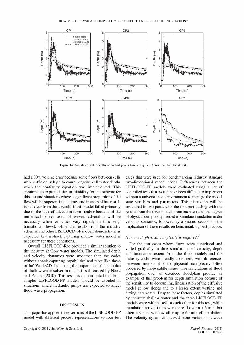
simulated by LISFLOOD-Roe are plotted at 5 s intervalsfor the first 30 s of the simulation in Figure 13. The modelperformed as expected, with a hydraulic jump developing infront of the building from 15 s onwards and a wake zone


behind the building from 20 s onwards. To compare theLISFLOOD-FP models and industry shallow water codes,water level time-series were recorded at the six control pointsin Figure 14, although neither LISFLOOD-ATS norLISFLOOD-ACC was expected to simulate this test caseadequately as they lack the necessary physics. LISFLOOD-ATS provided a smooth but inaccurate solution to the testwithout simulating the hydraulic jump, although the massconservation was the best of the three models. LISFLOOD-ACCwas the least accurate of the LISFLOOD-FPmodels and


0 100 200 3000

1

2

3

4

5

6CP1

Time (s)

Dep

th (

m)

Dep

th (

m)

Dep

th (

m)

Dep

th (

m)

Dep

th (

m)

Dep

th (

m)

0 100 200 3000

1

2

3

4

5

6CP2

Time (s)0 100 200 300

0

1

2

3

4

5

6CP3

Time (s)

Time (s) Time (s) Time (s)0 100 200 300

0

1

2

3

4

5

6CP4

0 100 200 3000

1

2

3

4

5

6CP5

0 100 200 3000

2

4

6

8

10CP6

Industry codesLISFLOOD−RoeLISFLOOD−ACCLISFLOOD−ATS

Figure 14. Simulated water depths at control points 1–6 on Figure 13 from the dam break test


had a 30% volume error because some flows between cellswere sufficiently high to cause negative cell water depthswhen the continuity equation was implemented. Thisconfirms, as expected, the unsuitability for this scheme forthis test and situations where a significant proportion of theflow will be supercritical at times and in areas of interest. Itis not clear from these results if this model failed primarilydue to the lack of advection terms and/or because of thenumerical solver used. However, advection will benecessary when velocities vary rapidly in time (e.g.transitional flows), while the results from the industryschemes and other LISFLOOD-FP models demonstrate, asexpected, that a shock capturing shallow water model isnecessary for these conditions.Overall, LISFLOOD-Roe provided a similar solution to

the industry shallow water models. The simulated depthand velocity dynamics were smoother than the codeswithout shock capturing capabilities and most like thoseof InfoWorks2D, indicating the importance of the choiceof shallow water solver in this test as discussed by Néelzand Pender (2010). This test has demonstrated that bothsimpler LISFLOOD-FP models should be avoided insituations where hydraulic jumps are expected to affectflood wave propagation.

DISCUSSION

This paper has applied three versions of the LISFLOOD-FPmodel with different process representations to four test


cases that were used for benchmarking industry standardtwo-dimensional model codes. Differences between theLISFLOOD-FP models were evaluated using a set ofcontrolled tests that would have been difficult to implementwithout a universal code environment to manage the modelstate variables and parameters. This discussion will bestructured in two parts, with the first part dealing with theresults from the three models from each test and the degreeof physical complexity needed to simulate inundation underversions scenarios, followed by a second section on theimplication of these results on benchmarking best practice.

How much physical complexity is required?

For the test cases where flows were subcritical andvaried gradually in time simulations of velocity, depthand inundation extent from the three models and theindustry codes were broadly consistent, with differencesbetween models due to physical complexity oftenobscured by more subtle issues. The simulations of floodpropagation over an extended floodplain provide anexample of this problem for depth simulation because ofthe sensitivity to decoupling, linearization of the diffusivemodel at low slopes and to a lesser extent wetting anddrying parameters. Despite these factors, depths simulatedby industry shallow water and the three LISFLOOD-FPmodels were within 10% of each other for this test, whileinundation arrival times were spread over a <6 min, butoften <3 min, window after up to 60 min of simulation.The velocity dynamics showed more variation between


J. NEAL ET AL.

the codes. The two simpler LISFLOOD-FP models,where the flow equations are decoupled in x and y,under-predicted the LISFLOOD-Roe velocity whenaligned with the grid and over-predicted on the diagonal,except when the time-step linearization takes effect inLISFLOOD-ATS. Although this is a limitation, beingunable to simulate symmetry was not an obvious problemin the real-world test cases and given the results fromJFLOW GPU not a problem that relates to physicalcomplexity. Nevertheless, if symmetry is essential thendecoupled schemes should be avoided. An ability tosimulate symmetry may thus be a theoretically interestingproperty for a hydraulic model, but one which may nothave great practical relevance.For the valley flooding following dam failure at 50m

resolution, maximum simulated depths were lower inLISFLOOD-ATS and -ACC, although the sensitivity tosubtle choices over how to sample the topography fromthe 10m DEM and the grid resolution of the model wereas important in determining local variations in depth andvelocity. LISFLOOD-Roe simulated later arrival timesand slower increases in water levels than the otherindustry shallow water models at 50m resolution,indicating the model had too much numerical diffusionat this scale, while being unable to simulate the wet/dryedges in a satisfactory manner. At 10m resolution,simulations from LISFLOOD-ACC and LISFLOOD-Roewere within the range of industry codes. Further work toimprove the scalability of the codes, particularly LISFLOOD-Roe, when applied to this test is needed. For LISFLOOD-ATS, the absence of inertia was evident around theregular transitions in slope along the reach. In percentageterms, the consistency in velocity simulation was similarto the consistency in simulation of depth, althoughvelocity was more sensitive to local DEM changes thandepth, which made this variable difficult to compare withthe industry codes due to uncertainties in topographicsampling.Simulation times varied dramatically between test cases,

although the LISFLOOD-FP model with the simplestphysical representation (LISFLOOD-ATS) required thelongest simulation time by between one and two orders ofmagnitude for all tests. The simulation times of LISFLOOD-Roe were consistent with the quicker explicit industryshallow water models in Néelz and Pender (2010), but theinertial model LISFLOOD-ACC was 3.2 times faster thanLISFLOOD-Roe for the flooding over an extended flood-plain. The flowover an extended floodplain test provides themost rigorous comparison of simulation times here becausesimulated depths and inundation extents were moreconsistent between the models in this test than the others.The simulation times for LISFLOOD-ATS are likely toseriously limit its suitability for large area, fine resolution orMonte Carlo type studies, even when the simulations areconsidered to be accurate enough for the task. Although notreported here, all the models were tested with inappropri-ately long time steps and found to be inaccurate, particularlyin terms of timings and velocities, meaning this should beavoided. This is especially relevant in the case of


LISFLOOD-ATS where a similar time step to that used inthe models with inertia will lead to inaccurate simulation.The high computational cost of LISFLOOD-ATS means itis tempting to use an adaptive time step similar to theshallow water models, whilst implementing a flow limiter toprevent the solution from oscillating. Hunter et al. (2005)provide a description of this approach; however, the flowlimiter should be avoided because it leads to a significantdeterioration in the quality of simulated wave propagation.At this point, it is useful to discuss the explicit diffusive

model results within the historical context of their use.These models were critical in highlighting the advantagesof 2D modelling of floodplain flows over 1D approaches(Horritt and Bates, 2002), while bringing flood simulationto a wider audience by being relatively easy to code,understand and visualise. Furthermore, the results hereand elsewhere (e.g. Yu and Lane, 2006; Tayefi et al.,2007; Hunter et al., 2008; Neal, 2009a) indicate that theinundation extents and depths typical of previousmapping work with these models would not changemarkedly if they were re-calculated using a more complexmethodology, at least for sites where flows vary graduallyand model time steps were appropriate. Explicit diffusivemodel also benefit from being simple; however, anyperception from previous work that this simplicity leadsto relative computational efficiency should be rejected inalmost all cases. Thus, in an operational context, theapproaches available for inundation simulation havemoved on from the LISFLOOD-ATS type formulation.The flow over a bump and dam break test cases require

the simulation of conditions that were expected tochallenge the two simpler LISFLOOD-FP formulations.Only LISFLOOD-Roe was able to simulate the flow overthe bump test case correctly. LISFLOOD-ACC could alsosimulate water overtopping the bump but only byincreasing the roughness, while LISFLOOD-ATS didnot overtop the bump as would be expected for a modelwhich lacks inertia. Thus, the diffusive and shallow watermodel results were consistent with the EA study, whilethe LISFLOOD-ACC results indicate that this model maybe suitable for similar test cases where flows aresubcritical and friction is greater than n= 0.03. Develop-ments to this scheme for urban applications should focuson methods to maintain stability at low friction withoutcompromising on speed, or the development of hybridmodels where the numerical scheme adapts to the flowconditions.LISFLOOD-Roe simulated similar dynamics to the

other shock capturing shallow water codes for the dambreak test case. LISFLOOD-ATS and LISFLOOD-ACCwere unable to simulate the hydraulic jump as expectedand should not be used if such features are essential to thesimulation, i.e. where the influence of the shocks extendsaway from their local vicinity and affects wavepropagation globally in the model. Where this occursappears easy to identify for LISFLOOD-ACC as in everysuch case examined here the mass balance errors from themodel become unacceptably large (see Table III). Hence,when applying the LISFLOOD-ACC model to test cases



where it was unable to emulate the full shallow watermodels depths and velocities to within ~10%, its massbalance error increased by many orders of magnitude. Ifwe conclude that the model is applicable to a smallerrange of scenarios than the full shallow water models,then mass balance would appear to be a good proxy fordetermining appropriateness and should thus always bereported. Furthermore, although LISFLOOD-ATS wasunable to simulate key aspects of the flow over a bumpand the dam break, the model remained stable andconserved mass for all the tests undertaken here unlike theother two models.

Implications for inundation model benchmarking

The previous discussion on model complexity highlightsthe difficulty of benchmarking complex models, whereaspects of model setup that might usually be considered asminor can obscure the headline differences between modelssuch as the type of solver used or physical complexity.Benchmarking is undoubtedly made easier by models thatshare common sub-routines and input data, such as the threeused here, but as this is not a practical solution for industrymodels. The tests conducted in the EA study established themagnitude of differences betweenmodels given a number oftest cases, which allowed model responses to be classifiedand approaches that simulated non-behavioural dynamics tobe identified. In terms of model suitability for variousapplications, the finding here support those of the EAmodelbenchmarking study (Néelz and Pender, 2010), except thatthe performance of LISFLOOD-ATS for velocity simula-tion was significantly better than the industry equivalents ofthis code and there was no industry implementation ofLISFLOOD-ACC. An important question is how significantthe choice of model is in relation to other factors, includingboth controllable model setup decisions (e.g. resolution,mesh type and the frequency with which results arerecorded) and model uncertainties (e.g. possible input flowdata and DEM errors).The valley filling test provides a convenient example of

how simple model setup decisions can have as muchimpact on hazard mapping as choosing between the threeLISFLOOD-FP models. Peak velocities at each controlpoint were short-lived to the extent that increasing the rateat which velocity was recorded from 1 min to 5 sincreased peak velocity by up to 8.9% at selected controlpoints. This has significant implications for risk assess-ment because methods that take infrequent snapshots ofmodel state variable may not capture maximum veloci-ties. Furthermore, maximum velocity and depth werebroadly coincident in time on the steeper sections of thedomain, with maximum depth occurring some time aftermaximum velocity on the shallower sections. Theimplication of this for hazard estimation is that theproduct of maximum simulated depth and maximumvelocity may overestimate hazard in particular locationsif these are determined separately. Also, since peakvelocity is short in duration, hazard will also changerapidly.


In addition to model setup issues that can be controlled,the significance of model choice in relation to the principalsources of uncertainty would be a useful addition to futurebenchmarking work. Here, it was relatively simple todemonstrate that simulations of the valley flooding eventwere as sensitive to the sampling of the 10m topography tocoarser resolutions as they were to model choice, and thatthe model had not converged on a grid-independentestimate of velocity by 10m. However, this should gofurther in future benchmarking work by evaluating thechoice of model given uncertainty in the elevation andinflow data typically used for the applications being tested.

CONCLUSIONS

Three two-dimensional hydraulic models with differentphysical representations have been benchmarked usingfour test cases. Well-known factors such as topographywere found to influence simulations, but a number of lessobvious factors also cause differences in simulations asgreat or greater than physical complexity. A number ofspecific conclusions can be made:

• Explicit diffusive type model required much longersimulation times than the models with inertia for the2–50m resolution applications considered here. Thisproblem cannot be solved by using fixed longer timesteps and a flow limiter because of the poor simulationof wave propagation with such methods.

• Decoupled schemes were unable to simulate symmetryover flat topography, although similar effects on theirregular topographies tested here were not identifiablegiven other factors. The simulation of symmetry istherefore an interesting technical test but may havelimited relevance to real world flows.

• For test cases with gradually varying flows, simulationsof velocity were surprisingly similar between the codesand usually as alike as depth in terms of % difference.This means that the simplified models may beappropriate for velocity simulation for a wider rangeof conditions than suggested by the EA study wheregradually varied subcritical flows are expected.

• For test cases where flows change gradually with time,the difference between models is only as large asdifferences caused by other modelling choices (e.g.topography sampling, recording of results, etc).

• The diffusive model LISFLOOD-ATS was the leastlike the other codes in the vicinity of slope transitionsfor the valley flooding following a dam failure test case.The momentum conservation over a bump test casedemonstrates how the diffusive model loses momentumtoo quickly when the DEM slope decreases.

• LISFLOOD-Roe as a pure first order in time and spacescheme simulated later arrival times and slowerincreases in water levels than the other shallow watermodels at the 50m resolution version of the valleyflooding test, while the CFL number had to be reducedin order to simulate the wet/dry edges in a stablemanner at 10m resolution.


J. NEAL ET AL.

• Simple decisions over often arbitrary modellingchoices, such as how frequently to record velocityand assumptions about depth velocity correlations, canhave greater impacts on hazard assessment thandecisions over model physical complexity.

• The simpler models were unable to simulate hydraulicjumps and wake zones, as expected.

• Rigorous control in benchmarking studies is difficult toachieve, especially when undertaken with multiplecodes and modellers.

• LISFLOOD-Roe was required when there weresubcritical to supercritical transitions in the flow thataffect the wave propagation, but unless contra-indicated by large mass errors LISFLOOD-ACC wasa faster alternative to a full shallow water model forgradually varied subcritical flows where domain-average friction typically exceeds n= 0.03.

LISFLOOD-Roe was applicable to the widest range offlow conditions, although it was inaccurate at the floodedge when adjacent velocity was high and grid resolutioncoarse. LISFLOOD-ACC was usually the quickest model,which would be particularly advantageous for real-timeinundation forecasting, Monte Carlo type analysis or largemodel applications. However, for conditions where thiscode was not physically suitable (e.g. low friction, Froudenumber> 1), the model became unstable and mass balanceerrors became large. For LISFLOOD-ATS, the ease of use,simplicity, stability and small mass errors may be desirablewhere the model is applied to cases where it is difficult tocheck model results, where only diffusive processrepresentation is required and where coarse resolutionmodels are needed. However, the computational cost willbe relatively high for typical strategic flood risk manage-ment applications.Through a rigorous series of benchmarks tests of 2D

hydraulic models, this paper is able to draw conclusionson the degree of physical complexity required to modelflood inundation. We show that for gradually varied flow,full shallow water models may be unnecessarily complex,and simpler, cheaper schemes, such as the inertial waveformulation in LISFLOOD-ACC, can perform just aswell, both in terms of velocity and depths. Moreover weshow that subtle modelling decisions can often have moreeffect on results than selecting a more physically complexmodel. The results of this study therefore provideadditional guidance to help 2D model users select theappropriate scheme for any given situation.

ACKNOWLEDGEMENT

Jeffrey Neal and Thomas Willis were funded by the FloodRisk Management Research Consortium, which issupported by grant number EP/F20511/1 from theEPSRC and the DEFRA/EA joint Research Program onFlood and Coastal Defence. We would like to thank thethree anonymous reviewers for their very helpfulcomments and suggestion, along with Jim Walker and


Sylvain Néelz for arranging access to the EA 2D modelbenchmarking data sets.

REFERENCES

Apel H, Aronica GT, Kreibich H, Thieken AH. 2009. Flood risk analyses-how detailed do we need to be? Natural Hazards 49: 79–98.

Aronica GT, Nasello C, Tucciarelli T. 1998. A 2D Multilevel Model forFlood Propagation in Flood Affected Areas. ASCE - Journal of WaterResources Planning and Management 124: 4.

Bates PD, De Roo APJ. 2000. A simple raster-based model for floodinundation simulation. Journal of Hydrology 236: 54–77.

Bates PD, Horritt MS, Fewtrell TJ. 2010. An simple inertial formulation ofthe shallow water equations for efficient two dimensional floodinundation modelling. Journal of Hydrology 387: 33–45.

Bradbrook KF, Lane SN, Waller SG, Bates PD. 2004. Two dimensionaldiffusion wave modelling of flood inundation using a simplified channelrepresentation. International Journal of River Basin Management 2:1–13.

Brufau P, García-Navarro P, Vázquez-Cendón ME. 2002. A numericalmodel for the flooding and drying of irregular domains. InternationalJournal for Numerical Methods in Fluids 39: 247–275.

Cobby DM, Mason DC, Davenport IJ. 2001. Image processing ofairborne scanning laser altimetry data for improved river floodmodelling. ISPRS Journal of Photogrammetry and Remote Sensing56(2): 121–138.

Crowder RA, Pepper AT, Whitlow C, Sleigh A, Wright N, Tomlin C.2004. Benchmarking of hydraulic river modelling software packages.SCHO0305BIXN-E-P. Environment Agency, Bristol.

Fewtrell TJ, Bates PD, Horritt M, Hunter NM. 2008. Evaluating the effectof scale in flood inundation modelling in urban environments.Hydrological Processes 22(26): 5107–5118.

Fewtrell TJ, Duncan A, Sampson CC, Neal JC, Bates PD. 2011.Benchmarking urban flood models of varying complexity andscale using high resolution terrestrial LiDAR data.. Physics andChemistry of the Earth 36(7–8): 281–291.

Gouldby B, Sayers P, Mulet-Marti J, Hassan MAAM, Benwell D. 2008. Amethodology for regional-scale flood risk assessment. Proceedings of theInstitution of Civil Engineers - Water Management 161: 169–182.

Guinot V, Soares-Frazao OS. 2006. Flux and source term discretization intwo-dimensional shallow water models with porosity on unstructuredgrids. International Journal for Numerical Methods in Fluids 50:309–345.

Hall JW, Dawson RJ, Sayers PB, Rosu C, Chatterton JB, Deakin R. 2003.A methodology for national-scale flood risk assessment. Proceedings ofthe Institution of Civil Engineers-Water and Maritime Engineering 156:235–247.

Hall JW, Manning LJ, Hankin RKS. 2011. Bayesian calibration of a floodinundation model using spatial data. Water Resources Research 47:W05529.

Hall JW, Sayers PB, Dawson RJ. 2005. National-scale assessment ofcurrent and future flood risk in England and Wales. Natural Hazards36: 147–164.

Horritt MS. 2000. Calibration of a two-dimensional finite element floodflow model using satellite radar imagery. Water Resources Research36(11): 3279–3291.

Horritt MS, Bates PD. 2001. Predicting floodplain inundation: raster-basedmodelling versus the finite-element approach. Hydrological Processes15(5): 825–842.

Horritt MS, Bates PD. 2002. Evaluation of 1D and 2D numerical modelsfor predicting river flood inundation. Journal of Hydrology 268(1–4):87–99.

Horritt MS, Di Baldassarre G, Bates PD, Brath A. 2007. Comparing theperformance of a 2-D finite element and a 2-D finite volume model offloodplain inundation using airborne SAR imagery. HydrologicalProcesses 21: 2745–2759.

Hunter NM, Bates PD, Neelz S, Pender G, Villanueva I, Wright NG,Liang D, Falconer RA, Lin B, Waller S, Crossley AJ, Mason DC.2008. Benchmarking 2D hydraulic models for urban flooding.Proceedings of the Institution of Civil Engineers-Water Management161(1): 13–30.

Hunter NM, Horritt MS, Bates PD, Wilson MD, Werner MGF. 2005.An adaptive time step solution for raster-based storage cellmodelling of floodplain inundation. Advances in Water Resources28: 975–991.



Lamb R, Crossley A, Waller S. 2010. A fast 2 d floodplain inundationmodel. Proceedings of the Institution of Civil Engineers - WaterManagement 162: 363–370.

Leopardi A, Oliveri E, Greco M. 2002. Two-dimensional modeling offloods to map risk-prone areas. ASCE Journal of Water ResourcesPlanning and Management 128(3): 168–178.

Lhomme J, Gutierrez-Andres J, Weisgerber A, Davison M, Mulet-Marti J,Cooper A, Gouldby B. 2010. Testing a new two-dimensional floodmodelling system: analytical tests and application to a flood event.Journal of Flood Risk Management 3(1): 33–51.

Liang D, Falconer RA, Lin BL. 2006. Comparison between tvd-maccormack and adi-type solvers of the shallow water equations.Advances in Water Resources 29: 1833–1845.

Liang D, Lin B, Falconer RA. 2007. Simulation of rapidly varying flowusing an efficient TVD- MacCormack scheme. International Journalfor Numerical Methods in Fluids 53(5): No. 3, 811–826.

McMillan HK, Brasington J. 2007. Reduced complexity strategiesfor modelling urban floodplain inundation. Geomorphology 90:226–243.

Mignot E, Paquier A, Haider S. 2006. Modeling floods in a dense urbanarea using 2 d shallow water equations. Journal of Hydrology 327:186–199.

Neal J, Bates P, Fewtrell T, Hunter NM, Wilson M, Horritt M. 2009a.Distributed whole city water level measurements from the Carlisle 2005urban flood event and comparison with hydraulic model simulations.Journal of Hydrology 368: 42–55.

Neal JC, Fewtrell TJ, Trigg MA. 2009b. Parallelisation of storage cellflood models using openmp. Environmental Modelling and Software24: 872–877.

Neal JC, Fewtrell TJ, Bates PD, Wright NG. 2010. A comparisonof three parallelisation methods for 2D flood inundation models.Environmental Modelling & Software 25(4): 398–411.

Neal J, Schumann G, Fewtrell T, Budimir M, bates P, Mason D.2011. Evaluating a new LISFLOOD-FP formulation with datafrom the summer 2007 floods in Tewkesbury, UK. Journal ofFlood Risk Management 4(2): 88–95.

Prestininzi P. 2008. Suitability of the diffusive model for dam breaksimulation: Application to a CADAM experiment. Journal of Hydrology361(1–2): 172–185:


Néelz S, Pender G. 2010. Benchmarking of 2D Hydraulic ModellingPackages. SC080035/SR2. Environment Agency, Bristol.

Roe P. 1981. Approximate Riemann Solvers, Parameter Vectors, andDifference-Schemes. Journal Of Computational Physics 43(2): 357–372.

Sanders BF. 2007. Evaluation of on-line dems for flood inundationmodeling. Advances in Water Resources 30: 1831–1843.

Schubert JE, Sanders BF, Smith MJ, Wright NG. 2008. Unstructuredmesh generation and landcover-based resistance for hydrodynamicmodeling of urban flooding. Advances in Water Resources 31(12):1603–1621.

Soares-Frazao S, Zech Y. 2002. Dam-break flow experiment: The isolatedbuilding test case. Available online at: http://www.impact-project.net/wp3_technical.htm

Stelling GS, Kernkamp HWJ, Laguzzi MM. 1998. Delft Flooding System:a powerful tool for inundation assessment based upon a positive flowsimulation. Hydroinformatics ’98, Babovic, Larsen (eds). Balkema:Rotterdam; 449–456.

Syme WJ. 1991. Dynamically linked two-dimensional/one-dimensionalhydrodynamic modelling programfor rivers estuaries and coastal waters.MEngSc thesis, University of Queensland, Australia.

Tayefi V, Lane SN, Hardy RJ, Yu D. 2007. A comparison of one- andtwo-dimensional approaches to modelling flood inundation overcomplex upland floodplains. Hydrological Processes 21(23):3190–3202.

Villanueva I, Wright NG. 2006. Linking Riemann and storage cell modelsfor flood prediction. Proceedings of the Institution of Civil Engineers,Journal of Water Management 159: 27–33.

Werner MGF. 2004. A comparison of flood extent modelling approachesthrough constraining uncertainties on gauge data. Hydrology and EarthSystem Sciences 8(6): 1141–1152.

Werner MGF, Hunter NM, Bates PD. 2005. Identifiability of distributedfloodplain roughness values in flood extent estimation. Journal ofHydrology 314(1–4): 139–157.

Wilson MD, Atkinson PM. 2007. The use of remotely sensed land coverto derive floodplain friction coefficients for flood inundation modelling.Hydrological Processes 21(26): 3576–3586.

Yu D, Lane SN. 2006. Urban fluvial flood modelling using a two-dimensional diffusion-wave treatment, part 2: Development of asub-grid-scale treatment. Hydrological Processes 20: 1567–1583.


http://www.impact-project.net/wp3_technical.htm

http://www.impact-project.net/wp3_technical.htm

how much physical complexity is needed to model flood inundation?

Documents