Paper Presented to the First International Workshop on Intelligent Finance – IWIF 13-14 December 2004, Melbourne, Australia

How Long is the Long Run? Evidence from the Foreign Exchange Market*

by

Kenneth Clements

Economics Program The University of Western Australia

Tel: (08) 6488 2898 Fax: (08) 6488 1016

Email: kclement@ecel.uwa.edu.au

and

Yihui Lan Economic Research Centre

Economics Program The University of Western Australia

Tel: (08) 6488 1368 Fax: (08) 6488 1016

Email: ylan@ecel.uwa.edu.au

Abstract

The aim of this paper is to estimate the length of the long run in the foreign exchange market. We do this by examining the link between exchange rates and relative prices, based on the implications of purchasing power parity (PPP) theory. Using a new approach, we test if the ratios of variances of exchange rates to prices are unity over all horizons, as implied by PPP. Through Monte Carlo simulations, we derive the variance ratios under the null of equal variances and examine the power and size of the test. We find evidence that PPP holds in the long run. While the long run based on the consumer prices appears to be “long”, about five years, the estimate of the long run based on the single good, Big Macs, is shorter (two years).

Keywords: foreign exchange market, purchasing power parity, long run, variance ratio.

* We would like to thank three anonymous referees of the IWIF1 for helpful comments. This research was supported by an ARC Linkage Grant with ACIL Tasman Consultancy, AngloGold Ashanti Australia Limited and the Western Australian Department of Industry and Resources as industry partners. The views expressed herein are not necessarily those of the supporting organizations.

1

1. Introduction

The concept of purchasing power parity (PPP) is deeply rooted in the minds of many economists (Dornbusch and Krugman, 1976). PPP theory states that prices across countries should be equal when converted to a common currency (absolute PPP), or less strictly, the change in the exchange rate should be equal to the difference between inflation at home and abroad (relative PPP). Empirically, however, there is much heated debated regarding whether PPP holds. Professional confidence in PPP dipped after the publication of the paper “The Collapse of Purchasing Power Parities during the 1970s” by Frenkel (1981). Over the past three decades, the research devoted to PPP has been increasing dramatically and there is now general consensus that PPP is not a theory of short-term exchange rate determination, but it does offer a long-run equilibrium relationship between relative prices and exchange rates, at least for the major currencies.

To measure the extent of professional interest in PPP, we search for the total number of

journal articles containing the phrase “purchasing power parity” in Econlit, a widely-used economic indexing database produced by the American Economic Association.1 For comparison we also search for another five terms. The search results for each term are categorized into three sub-periods and are reported in Figure 1. The left-hand axis uses a logarithmic scale, so that the change in the height of the bars indicates the exponential rate of growth. The right-hand axis gives the growth rate, on an annual basis, for each topic. It can be seen that the number of articles on PPP has grown at an average rate of 15 percent p.a., second only to foreign direct investment. This growth rate clearly reflects the strong expansion of research interest in PPP over the past three decades, so that PPP research can now be described as “exploding” rather than “collapsing”.

Financial markets are also interested in PPP as a practical approach to valuing currencies and

in making international price comparisons. However, PPP does not usually hold exactly and there are always prolonged deviations from PPP; for details, see surveys by Froot and Rogoff (1995),

FIGURE 1

THE GROWTH OF ECONOMIC RESEARCH

7.7

15.2

20.8

10.0

14.6

10.2

10

100

1,000

10,000

100,000

Infla

tion

Une

mpl

oym

ent

Inte

rest

rate

Exch

ange

rate

Fore

ign

dire

ctin

vestm

ent

Purc

hasin

gpo

wer

par

ity

Num

ber o

f Jou

rnal

Arti

cles

6

9

12

15

18

21A

nnua

l Gro

wth

Rat

e(p

erce

nt p

. a.)

1974-19831984-19931994-2003

1 The material in this paragraph updates Lan (2004).

2

Rogoff (1996), Sarno and Taylor (2002), and Taylor and Taylor (2004). The focus of recent research on PPP is on the length of time taken to establish the PPP relationship between exchange rates and prices, that is, the length of the long run. This paper proposes a new test to examine this topic, based on the ratio of the variance of exchange rates to that of relative prices. Unlike previous tests of PPP, which involve traditional methods of regression or cointegration analysis for pairs of countries, our approach deals with all countries simultaneously.2 The organisation of the paper is as follows. Section 2 provides theoretical background to the analysis. Section 3 presents the data and empirical variance ratios of exchange rates and relative prices. In Section 4, we simulate the confidence band of the variance ratios under the null hypothesis of equal variances under PPP. Section 5 examines the power and size of the new variance ratio test. We conduct a sensitivity analysis in Section 6 and compare the estimate of the length of the long run based on consumer price indexes with that based on the Big Mac Index from The Economist magazine. The final section concludes.

2. Theoretical Foundations

Let tS be the nominal exchange rate in year t, defined as the domestic currency cost of a unit of foreign exchange, and tP and *

tP be the domestic and foreign price levels. Relative PPP then provides a strong link between the exchange rate and prices:

(1) t ts r∆ = ∆ , where t t t 1s logS logS −∆ = − is the log-change in S, and * *

t t 1 t t 1r log (P / P ) log (P / P )− −∆ = − is the difference between inflation at home and abroad. In words, equation (1) states that the change in the exchange rate equals the inflation differential. Clearly equation (1) implies that

t tvar ( s ) var ( r )∆ = ∆ , so that the volatility of exchange rates and prices coincide.

Consider equation (1) applied to the transition from year t-2 to t-1, so that t 1 t 1s r− −∆ = ∆ . If we add both sides of this equation to equation (1) we obtain

* *t t 2 t t 2 t t 2log S log S log (P / P ) log (P / P )− − −− = − , which we write as (2) (2)

t ts r∆ = ∆ , where (2) 1t t t 22s (logS logS )−∆ = − is the annualised log-change in S and [(2) 1

t t t 22r log(P / P )−∆ = * *t t 2log (P / P )− − is the corresponding annualised inflation differential. A similar argument

establishes that for any horizon m, (2) (m) (m)

t ts r∆ = ∆ , where, e.g., (m) 1

t t t mms (logS logS )−∆ = − . If we define the variance ratio as (m) (m)(m) var[ s ]/ var[ r ]φ = ∆ ∆ , equation (2) then implies (m) 1φ = for any value of m.3 In

2 One exception is Manzur (1990, 1993), which also avoid taking pairs of countries in isolation. But our approach is based on the ratio of two variances, while Manzur is based on Divisia index numbers. 3 This variance ratio is to be distinguished from the variance ratio proposed by Cochrane (1988), which is used to detect a unit root in a time series. According to Cochrane, if the ratio of the variance of the kth to the first differences is greater than k, there exists a unit root.

3

other words, PPP implies that over horizons, the variance of the exchange rates is the same as that of the inflation differential.4

If PPP does not hold, then the change in the inflation-adjusted, or, real, exchange rate,

t ts r∆ − ∆ , is non-zero and equations (1) and (2) have to be modified to (3) t t ts r∆ = ∆ + ε , (m) (m) (m)

t t ts r∆ = ∆ + ε , where tε is the one-year change in the real exchange rate and

(4) m 1

(m)t t j

j 0

1m

−

−=

ε = ε∑

is the corresponding annualised change over horizon m. As an illustrative example, consider the case in which real exchange rate changes are orthogonal to inflation differentials, have a constant variance 2

εσ and are independent over time.5 Equation (4) then implies

(5) 2

(m)var[ ]mεσε = ,

and the variance ratio becomes

(6) (m)

(m)var[ ]

(m) 1var[ r ]

εφ = +

∆

2

(m)1m var[ r ]

εσ= +× ∆

.

If we make the reasonable assumption that (m)

mlim var[ r ]→∞ ∆ is finite, then equation (6) reveals that when the horizon m→∞ , (m) 1φ → , so at long horizons we are back to the original case whereby the exchange rate and relative prices have the same volatility.

3. Exchange Rates and Prices Across Time and Countries

This section investigates the behaviour of exchange rates and prices over time and over a substantial number of countries. We denote countries by a c subscript and obtain the exchange rate and Consumer Price Index (CPI) data from the International Financial Statistics for 4 We are not testing directly for PPP, which involves an examination of the comovement of logarithmic of variables tS , tP and *

tP . Rather we test it indirectly via its volatility implications. Note that while PPP implies equal variances and that (m) 1φ = is not inconsistent with PPP, we cannot conclude that (m) 1φ = always implies PPP. This is a qualification to our approach. 5 The assumption that real exchange rate changes, ε , are independent over time requires some comment. This assumption implies that the real exchange rate has a unit root: * *

t t t t 1 t 1 t 1 tlog (P / S P ) log (P / S P )− − −= + ε . While such an assumption may appear to be strong, in fact it does not do too much violence to the truth (e.g., Meese, 1990, Mussa, 1979, 1990), and can be justified on the basis of the foreign exchange market being near efficient. However, it is to be emphasised that the above is just an example and in what follows, we make no a priori assumption about the behaviour of real exchange rates.

4

c 1, ..., 50= countries and t 1974 2004= − with the US as the base country.6 Thus the maximum value of the differencing span here is maxm 2004 1974 30= − = years. For all countries and years, we plot cts∆ against ctr∆ in panel A of Figure 2. It is obvious that many of the points are of a considerable distance from the o45 line and are thus not supportive of PPP. Panel B of Figure 2 contains a scatter plot of the annualized 30-year changes, (30)

cts∆ and (30)ctr∆ .7 As the points are

now much “closer” on average to the o45 line, visually there seems to be impressive support for PPP in Panel B. As we can interpret the 30-year changes as reflecting the long run, when all adjustments are complete, it can be seen why it is that many authors have emphasised that PPP only applies over the longer term, not on a year-to-year basis.

To measure the dispersion of the points around the o45 line in a given panel of Figure 2,

we use the root-mean-squared error (RMSE), which has the property that if all points lie on the o45 line, the RMSE is zero. As can be seen from Panel A, which corresponds to annual changes, the RMSE is about 12 percent. The changes over the entire 30-year period (Panel B) give the much lower RMSE of about 2 percent. This reinforces the discussion in the previous paragraph that PPP holds better in the long run.

We have compared exchange rates and prices over one- and 30-year horizons. As can be

seen from panel A of Figure 2, for m = 1 the variance of exchange rates seems to be larger than that of relative prices with annual changes. That is, the scatter in Panel A is substantially “higher” than its “width” (the scales are the same on both axes). By contrast, in Panel B of the figure (m = 30) the two variances seems to be more or less the same. This indicates that in the short run (1) 1φ > , while for the long run (30) 1φ ≈ . This result seems to be not inconsistent with equation (6). The reason for (1) 1φ > is the existence of 2

εσ , which reflects the variability of real exchange rates, so that 2(1) 1 / var[ r] 1εφ = +σ ∆ > .

As we know the two “end points” for the function (m)φ , (1) 1φ > and (30) 1φ ≈ , it is

natural to ask, what is the nature of the transition path in going from the short run to the long run? What period of time has to elapse until the ratio effectively hits unity? One way to investigate this issue is to analyse the variance ratio (m)φ for 1 m 30< < . To do this, for a given value of m we average over all countries and years to yield an estimate of (m)φ .8 The solid line in Figure 3 6 The data we use are annual inflation rates for the 50 countries and the exchange rates in the first quarter of each year from 1974 to 2004. The countries are selected from the International Financial Statistics on the following basis: (i) CPIs are available for all years. The only exception to this rule is Cameroon whose CPI in 2004 is unavailable. We omit that country for that year. (ii) Exchange-rates data for all periods are available. The exceptions to this rule are EU member countries whose exchange rates after 1999 are unavailable and the Soloman Islands whose 2004 rate is not available. For these countries, in the computation of var[ s]∆ and

var[ r]∆ we delete the pair of (m)cts∆ and (m)

ctr∆ whenever we cannot obtain either (m)cts∆ or (m)

ctr∆ . For eaanple, there are only 38 pairs of observations when m=30 mainly because of the missing exchange rates for EU countries. (iii) The one-year changes, ts∆ and tr∆ , are less than 80 percent in absolute value. In addition, it is to be noted that in 1993, the currencies of five African countries, Burkina Faso, Cameroon, Cote d’Ivoire, Niger, and Senegal jointly depreciated by about 65 percent. This is shown as the several points at the top end near the vertical axis in Panel A of Figure 2. 7 Similar analyses are provided in Lothian (1985) and Obstfeld (1995). 8 It is to be noted that all data used in this paper involve non-overlapping observations.

5

-40

-20

0

20

40

60

80

-40 -20 0 20 40 60 80

-40

-20

0

20

40

60

80

-40 -20 0 20 40 60 80

FIGURE 2

CHANGES IN EXCHANGE RATES AND RELATIVE PRICES FOR 50 COUNTRIES, 1974-2004 (Annualised logarithmic changes)

A. Short run (all 50 countries, 30 years)

B. Long run (38 countries)

Note: There are only 38 observations in panel B due to missing observations, which are mainly

associated with EU countries.

45o line

Inflation 100r )31(

c ×∆

Exchange rate100s )31(

c ×∆

RMSE = 1.71%

Inflation 100rct ×∆

45o line

Exchange rate100sct ×∆

RMSE = 12.24%

6

FIGURE 3

VARIANCES OF EXCHANGE RATES AND RELATIVE PRICES

0.0

0.5

1.0

1.5

2.0

2.5

3.0

3.5

4.0

1 6 11 16 21 26

ObservedFitted

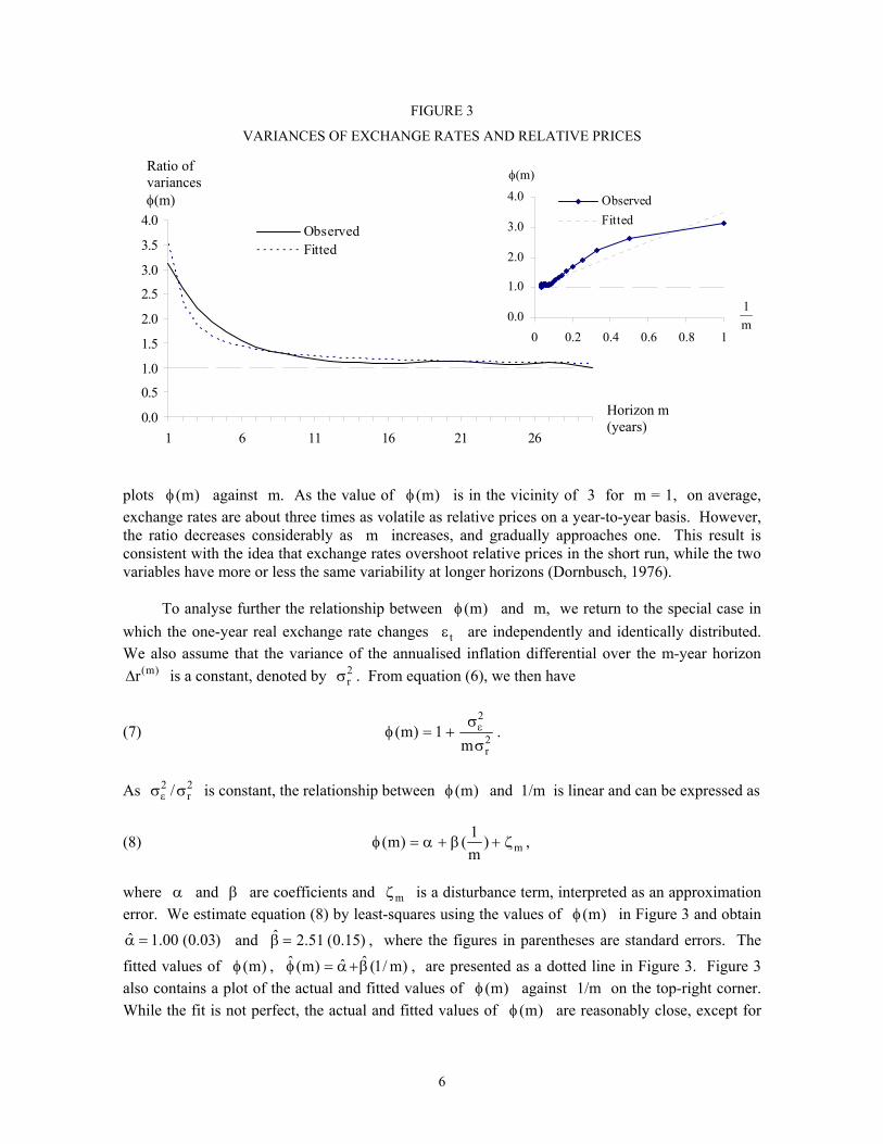
plots (m)φ against m. As the value of (m)φ is in the vicinity of 3 for m = 1, on average, exchange rates are about three times as volatile as relative prices on a year-to-year basis. However, the ratio decreases considerably as m increases, and gradually approaches one. This result is consistent with the idea that exchange rates overshoot relative prices in the short run, while the two variables have more or less the same variability at longer horizons (Dornbusch, 1976).

To analyse further the relationship between (m)φ and m, we return to the special case in

which the one-year real exchange rate changes tε are independently and identically distributed. We also assume that the variance of the annualised inflation differential over the m-year horizon

(m)r∆ is a constant, denoted by 2rσ . From equation (6), we then have

(7) 2

2r

(m) 1m

εσφ = +σ

.

As 2 2

r/εσ σ is constant, the relationship between (m)φ and 1/m is linear and can be expressed as

(8) m1(m) ( )m

φ = α + β + ζ ,

where α and β are coefficients and mζ is a disturbance term, interpreted as an approximation error. We estimate equation (8) by least-squares using the values of (m)φ in Figure 3 and obtain ˆ 1.00 (0.03)α = and ˆ 2.51 (0.15)β = , where the figures in parentheses are standard errors. The

fitted values of (m)φ , ˆ ˆˆ(m) (1/ m)φ = α+β , are presented as a dotted line in Figure 3. Figure 3 also contains a plot of the actual and fitted values of (m)φ against 1/m on the top-right corner. While the fit is not perfect, the actual and fitted values of (m)φ are reasonably close, except for

Ratio of variances φ(m)

Horizon m (years)

φ(m)

1m

0.0

1.0

2.0

3.0

4.0

0 0.2 0.4 0.6 0.8 1

ObservedFitted

7

the initial few years. Both estimated parameters are significant and the estimated value of α is not significantly different from its theoretical value of unity. When the horizon is m 1= , the predicted variance ratio is ˆ ˆˆ(1) 3.51φ = α+β = , implying that on a one-year basis exchange rates are about three and a half times as volatile as the corresponding inflation differential, which is not inconsistent with the previous discussion. For horizons greater than five years, the predicted variance ratio is very close to its actual counterpart, providing evidence that the assumption of constant variances of exchange rates changes and inflation differentials are not grossly contradicted by the data.9

Consider the effects of a one-year shock to real exchange rate t 0ε > . From equation (3), the nominal rate changes one-for-one in the same year. But as we proceed through time and if there are no subsequent shocks, the impact of this tε dies out. That is, from equation (4), for t t′> ,

(m)t tt / m′ε = ε < ε for all horizons m 1> . Let m′ be the horizon for which (m )

t 0′′ε ≈ , so that the

real exchange rate has effectively returned to its pre-shock value. We shall call m′ “the long run”. As (m )var[ ] 0′ε → , (m ) 1′φ → . Figure 3 reveals that (m)φ gradually declines to a value in the vicinity of one. The important question is, at what horizon m′ can the variance ratio be considered to be sufficiently “close” to unity so that this m′ can be regarded as the long run? We will analyse this question in the next section.

4. Measuring the Long Run

As explained in Section 2, relative PPP gives the relationship between exchange-rate changes and relative-price changes. The variance ratio being one corresponds to the idea that there is one-for-one co-movement in these two variables. We thus suppose that the data-generating process is as follows:

(9) (m) (m) (m)

0 ct ct ctH : s r∆ = ∆ + ε . To find out the length of the long run, we need to compare the data-based variance ratio plotted in Figure 3 with the distribution of the variance ratio under the null of equal variances of (m)

cts∆ and (m)ctr∆ . If for a particular value of m the empirical variance ratio falls into the 95 percent

confidence band and stays there, we can conclude that the value of m constitutes the long run of the foreign exchange market.10

We derive the distributions of (m)φ using the following Monte Carlo approach. The first

equation of (3) for country c defines the one-year residuals ct ct cts rε = ∆ − ∆ , and the corresponding m-year concept (m) (m) (m)

ct ct cts rε = ∆ − ∆ . As the sample period is 1974-2004, there are 30 annual changes, i.e., for m=1. In general for horizon m, there are 31-m observations. We apply the bootstrap approach to draw from these residuals. In simulation trial k ( k 1, ... , 1000= ), we draw 31 m− residuals for country c and denote them by ct,kε . Since the data-generating process is equation (9), the exchange rate change in trial k is given by adding the data-based 9 In fact, the constancy of β in equation (8) is implied by the weak assumption that the ratio of the variances is constant. 10 This value of m was refereed to as m′ in the previous section.

8

(m)ctr∆ to (m)

ct,kε , so that (m) (m)(m)ctct,k ct,ks r∆ = ∆ + ε . The variance ratio in trial k is thus

(m)* (m)k k(m) var[ s ]/ var[ r ]φ = ∆ ∆ . As (m) (m) (m) (m) (m)

k k kvar[ s ] var[ r ] var[ ] cov[ r , ]∆ = ∆ + ε + ∆ ε , the simulated variance ratio can be written as

(10) (m) (m) (m)

* k kk (m)

var[ ] cov[ r , ](m) 1

var[( r) ]ε + ∆ ε

φ = +∆

.

As the error terms in the above simulation, (m)

ct,kε , are bootstrapped from the data-based residuals,

which are the exchange-rate changes from equation (9), the bootstrapped exchange rates, (m)ct,ks∆ ,

are related to the observed distribution of (m)cts∆ . In addition, as in each trial k we fix the inflation

differential at its data-based values, (m)ctr∆ , the simulated variance ratios *

k (m)φ will be scattered around their observed counterparts (m)φ and thus reflect the distribution of the data-based ratio

(m)φ . But as discussed previously, if PPP holds for all horizons, real exchange rate changes are negligible, i.e., (m)

t 0ε ≈ for any m. To obtain the confidence band of the variance ratios under the null, we thus need to remove the effects of these real exchange rate changes. We do so by subtracting the second term on the right-hand side of equation (10) from *

k (m)φ to obtain the variance ratio under the null, denoted by k (m)φ . Finally, the 1,000 values of k (m)φ are sorted in the ascending order, and the 25th and 975th values, denoted by L (m)φ and U (m)φ , are the lower and upper bounds of the variance ratios under the null.

In Figure 4, we plot L (m)φ and U (m)φ for horizons m 1, ... , 30= , together with the data-based variance ratios. As can be seen, the data-based ratio falls into the confidence band under the null when m 5> . Thus after about five years, changes in exchange rates and relative prices have more or less the same variability, so that the long run of the foreign exchange market is about five years.

FIGURE 4 VARIANCE RATIOS AND THE CONFIDENCE INTERVAL

0.0

0.5

1.0

1.5

2.0

2.5

3.0

3.5

1 6 11 16 21 26

95% CI lower bound 95% CI upper bound

Data-based variance ratio

Horizon m (years)

Ratio of variances φ(m)

9

5. The Power and Size of the Variance Ratio Test

In this section we examine the reliability of our test by investigating its power -- the percentage of cases the null is rejected when the null is in fact false. In addition, the size of the test is obtained by examining the power of the test under the null.

The null hypothesis of equal variances is described in equation (9). There are two kinds of

alternative hypothesis corresponding to unequal variance when PPP does not hold. One is that the error terms (m)

ctε do not approach zero over longer horizons, so that the impact of the second term in equation (10) can not be ignored when m increases. The other kind of alternative is the slope coefficient in the data-generating process 1β ≠ , i.e.,

(11) (m) (m) (m)

1 ct ct ctH : s r∆ = β∆ + ε , where 1β ≠ . We will examine the test power in this case when the exchange rate under or over shoots inflation ( 1β < , 1β > ).

We proceed by specifying a value of β in equation (11) and in the kth ( k 1, ... , 1000= ) trial, use bootstrapped residuals from the first equation in (3), as before, denoted by ct,kε . Equation

(4) then defines (m)ct,kε , as before. As discussed in Section 3, the variance of (m)

ctε is sufficiently small only after the long run and the long estimate is about five years as shown in Section 4. Accordingly, for horizons m 5≤ the shock terms will be big as compared to those in the long run if we bootstrap them from the large data-based error terms. Thus for m 5≤ we bootstrap the error terms from the residuals according to (5)

ctε , and for m 5> the error terms are bootstrapped from the data-based residuals, (m)

ctε . Then the exchange-rate changes are generated via equation (11) as (m) (m)(m)

ctct,k ct,ks r∆ = β∆ + ε . Finally, as before we calculate the variance ratio after the removal of the error effect to obtain k (m)φ . The percentage of cases that k (m)φ falls outside the confidence band of the variance ratio under the null, [ ]L U(m), (m)φ φ , gives the power of the test.

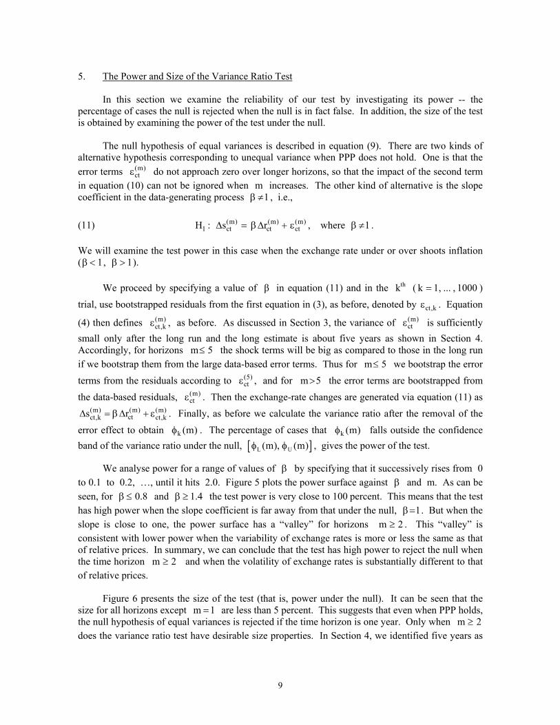
We analyse power for a range of values of β by specifying that it successively rises from 0 to 0.1 to 0.2, …, until it hits 2.0. Figure 5 plots the power surface against β and m. As can be seen, for 0.8β ≤ and 1.4β ≥ the test power is very close to 100 percent. This means that the test has high power when the slope coefficient is far away from that under the null, 1β= . But when the slope is close to one, the power surface has a “valley” for horizons m 2≥ . This “valley” is consistent with lower power when the variability of exchange rates is more or less the same as that of relative prices. In summary, we can conclude that the test has high power to reject the null when the time horizon m 2≥ and when the volatility of exchange rates is substantially different to that of relative prices.

Figure 6 presents the size of the test (that is, power under the null). It can be seen that the

size for all horizons except m 1= are less than 5 percent. This suggests that even when PPP holds, the null hypothesis of equal variances is rejected if the time horizon is one year. Only when m 2≥ does the variance ratio test have desirable size properties. In Section 4, we identified five years as

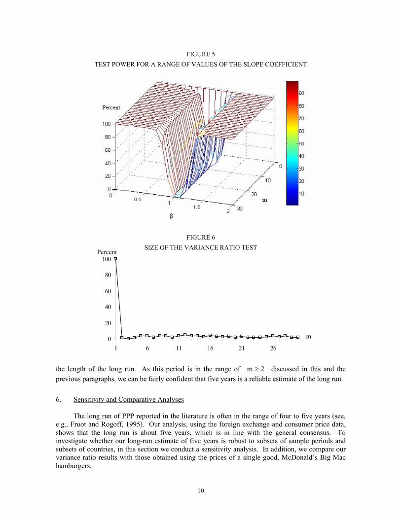
10

FIGURE 5 TEST POWER FOR A RANGE OF VALUES OF THE SLOPE COEFFICIENT

FIGURE 6 SIZE OF THE VARIANCE RATIO TEST

0

20

40

60

80

100

1 6 11 16 21 26

the length of the long run. As this period is in the range of m 2≥ discussed in this and the previous paragraphs, we can be fairly confident that five years is a reliable estimate of the long run.

6. Sensitivity and Comparative Analyses

The long run of PPP reported in the literature is often in the range of four to five years (see,

e.g., Froot and Rogoff, 1995). Our analysis, using the foreign exchange and consumer price data, shows that the long run is about five years, which is in line with the general consensus. To investigate whether our long-run estimate of five years is robust to subsets of sample periods and subsets of countries, in this section we conduct a sensitivity analysis. In addition, we compare our variance ratio results with those obtained using the prices of a single good, McDonald’s Big Mac hamburgers.

Percent

m

11

We first examine the variance ratios for a sub-set of 21 OECD countries included in our sample. Panel A of Figure 7 shows that the long run for OECD is about four years. Panel B gives an estimate of six years for the remaining 29 countries. While these results are quire similar to the previous estimate of five years, OECD exchange rates are much more volatile than those of the remaining countries. An examination shows that this is mostly caused by the high variability of the OECD rates in the mid-1980s when the US dollar considerably appreciated and then fell.

Next, we divide the whole sample period into three sub-periods, 1974-1984, 1984-1994, and

1994-2004. The estimates of long run corresponding to each of the three decades are 6, 4, and 4 years, as shown in panels A, B and C of Figure 8. A comparison of the three graphs reveals that in terms of the one-year changes (the first point in each graph), the exchange rates are more volatile in the sub-period of 1984-1994 than the other two sub-periods. It is also to be noted that exchange-rate volatility was smallest in the most recent decade.

FIGURE 7 VARIANCE RATIOS FOR SUBSETS OF COUNTRIES

A. 21 OECD countries

0

1

2

3

4

5

6

1 6 11 16 21 26

B. The rest 29 countries

0

1

2

3

4

5

6

1 6 11 16 21 26

Note: The legend is the same as in Figure 4.

FIGURE 8 VARIANCE RATIOS FOR SUB-PERIODS

A. 1974-1984 B. 1984-1994

C. 1994-2004

0

1

2

3

1 3 5 7 9

0

1

2

3

1 3 5 7 90

1

2

3

1 3 5 7 9

Note: The legend is the same as in Figure 4.

m

Percent Percent

m

Percent Percent Percent

m m m

12

The CPIs used above refer to the cost of market basket in each country. As these baskets differs from one country to another, we are not really comparing like with like. To better control for differing market baskets, we redo the analysis with an identical basket by using the famous Big Mac Index (BMI) published by The Economist magazine. This index is based on the prices of a universal good -- a McDonalds’ Big Mac hamburger, which is produced in about 180 countries in the world with almost identical ingredients. The Economist claims that the BMI is the “the world's most accurate financial indicator to be based on a fast-food item” (The Economist website). Several studies (Cumby, 1996, Lan, 2004, Parsley and Wei, 2003) find that the half-life estimates of the Big Mac PPP are shorter than those based on other price indices.

We use Big Mac prices in 24 countries and the US, and the corresponding 24 exchange rates versus the US dollar, for the period of 1994 to 2004 and Panel B of Figure 9 presents the variance ratio.11 For comparison we also reproduce Figure 4 in Panel A of Figure 9. With the BMI, the variance ratio falls into the 95 percent confidence band after about two years. This result is in agreement with the previously-mentioned studies that find, relative to CPI, a faster adjustment to PPP when Big Macs are used.

7. Concluding Remarks

According to purchasing power parity, a country’s exchange rate equals the ratio of prices at

home to those abroad, so that the proportionate change in the exchange rate equals the inflation differential. As such sharp hypotheses are rare in economics, it is not surprising that PPP has generated substantial controversy over a lengthy period. Among the contentious issues involving PPP, three can be highlighted. The first is the question of what causes what – does higher inflation at home lead to a depreciation of the exchange rate, or does causality go in the opposite direction? The second issue involves the period over which PPP can be expected to hold -- a day, a year, a decade, etc. Third, exactly what prices does the theory refer to -- consumer prices, GDP deflators, wages, or some individual commodities prices?

FIGURE 9

VARIANCE RATIOS WITH THE CPI AND THE BIG MAC DATA

A. The CPI B. The BMI

0.0

0.5

1.0

1.5

2.0

2.5

3.0

3.5

1 6 11 16 21 26

0.0

0.5

1.0

1.5

2.0

2.5

3.0

3.5

1 2 3 4 5 6 7 8 9 10

Note: The legend is the same as in Figure 4.

11 See Lan (2004) for details of the data.

φ(m) φ(m)

0.90

0.951.00

1.051.10

1 2 3

13

In this paper we have explored the meaning of the length of time required for PPP to hold. We used the idea that if exchange rates are proportional to relative prices, then the volatility of those two variables coincides. On a year-to-year basis, exchange rates are usually much more variable than prices; while as the time horizon increases to, say, a decade, the two variables tend to have a similar variance. In other words, PPP holds in the long run, but not the short run. We provided a new way of measuring exactly the length of the long run by examining the ratio of the variance of exchange rates to that of relative prices for various time horizons. This idea forms the basis of a new test of PPP, the variance ratio test. According to the test, the horizon for which the variance ratio falls close to unity and stays there, is the long run in so far as PPP is concerned.

We applied the variance ratio test to a large number of countries over the past three decades

and estimated that the long run was about five years. An investigation of the power of the new test reveals that its performance was at least satisfactory, especially for large departures from the null hypothesis. The size properties of the test were also satisfactory.

A long run of five years means that after this period has elapsed, exchange rates fully adjust

to relative prices. This result agrees with the general consensus of the long run estimate reported in the literature. We investigated the sensitivity of our result by (i) dividing countries into two groups -- OECD countries and the rest; and (ii) examining the data for three sub-periods. It is found that the results do not alter much. We also applied the methodology to the price of an individual good -- Big Mac hamburgers rather than Consumer Price Indexes -- and found that the Big Mac prices lead to a shorter long run of about two years.

Exchange rates are notoriously volatile and much research has been devoted to evaluating

approaches to forecasting exchange rates. Until recently, the consensus view was that the random walk model was an unbeatable way to predict future exchange rates (Meese and Rogoff, 1983, Frankel and Rose, 1995, Rogoff, 1999). But of course even if the random walk is the best available approach, needless to say that does not necessarily implies forecasts that are particularly accurate. More recently, however, research has shown that for medium to long horizons PPP beats the random walk (Kong, 2000, Lan, 2004, Simpson and Grossmann, 2004). Our paper in providing further evidence in favour of PPP and the length of the long run may thus contribute to further improvements of exchange rate forecasts.

References Cochrane, J. H. (1988). “How Big in the Random Walk in GNP?” Journal of Political Economy

96: 893-920. Cumby, R. E. (1996). “Forecasting Exchange Rates and Relative Prices with the Hamburger

Standard: Is What You Want What You Get with McParity? ” NBER Research Paper 5675. Dornbusch, R. (1976). “Expectations and Exchange Rate Dynamics.” Journal of Political Economy

84: 1161-76. Dornbusch, R. and P. Krugman (1976). “Flexible Exchange Rates in the Short Run.” Brookings

Papers on Economic Activity 3: 537-75. Frankel, J. A. and A. Rose (1995). “A Survey of Empirical Research on Nominal Exchange Rates.”

Chapter 33 in E. Grossman and K. Rogoff (eds) The Handbook of International Economics. Vol. 3. Amsterdam: North Holland. Pp. 1689-1729.

Frenkel, J. A. (1981). “The Collapse of Purchasing Power Parity during the 1970’s.” European Economic Review 16: 145-65.

14

Froot, K. A. and K. Rogoff (1995). “Perspectives on PPP and Long-Run Real Exchange Rates.” In G. Grossman, and K. Rogoff (eds) Handbook of International Economics. Amsterdam: North-Holland Press. Pp. 1647-88.

Kong, Q. (2000). “Predictable Movements in Yen/DM Exchange Rates.” International Monetary Fund Working Paper 00/143.

Lan, Y. (2004). “Equilibrium Exchange Rates and Currency Forecasts: A Big Mac Perspective.” Unpublished manuscript, Economics Program, The University of Western Australia.

Lothian, J. R. (1985). “Equilibrium Relationships between Money and other Economic Variables.” American Economic Review 75: 828-35.

Manzur, M. (1990). “An International Comparison of Prices and Exchange Rates: A New Test of Purchasing Power Parity”. Journal of International Money and Finance 9: 75-91.

Manzur, M. (1993). Exchange Rates, Prices and World Trade: New Methods, Evidence and Implications. London: Routledge.

Meese, R. (1990). “Currency Fluctuations in the Post-Bretton Woods Era.” Journal of Economic Perspectives 1: 117-34.

Meese, R. and K. Rogoff (1983). “Empirical Exchange Rate Models of the Seventies: Do They Fit Out of Sample?” Journal of International Economics 14: 3-24.

Mussa, M. (1979). “Empirical Regularities in the Behaviour of Exchange Rates and Theories of the Foreign Exchange Market.” Carnegie-Rochester Series on Public Policy 11: 9-58.

Mussa, M. (1990). Exchange Rates in Theory and Reality. Essays in International Finance No. 179, Princeton University.

Obstfeld, M. (1995). “International Currency Experience: New Lessons and Lessons Relearned.” Brookings Papers on Economic Activity 1: 119-220.

Parsley, D. C. and S.-J. Wei (2003). “A Prism into the PPP Puzzles: The Micro-foundations of Big Mac Real Exchange Rates.” NBER Working Paper No. w10074.

Simpson, M. R. and A. Grossmann (2004). “Can a Relative Purchasing Power Parity-based Model Outperform a Random Walk in Forecasting Shot-term Exchange Rates?” Unpublished Working paper, Department of Economics and Finance University of Texas – Pan American. Available at http://207.36.165.114/NewOrleans/Papers/7101656.pdf.

Rogoff, K. (1996). “The Purchasing Power Parity Puzzle.” Journal of Economic Literature 34: 647-68.

Rogoff, K. (1999). “Monetary Models of Dollar/Yen/Euro Nominal Exchange Rates: Dead and Undead?” The Economic Journal 109: F655-G659.

Taylor, M. P. and L. Sarno (2004). “International Real Interest Rate Differentials, Purchasing Power Parity and the Behaviour of Real Exchange Rates: The Resolution of a Conundrum." Journal of Finance and Economics 9: 15-23.

Taylor, A. and M. P. Taylor (2004). “The Purchasing Power Parity Debate.” Journal of Economic Perspectives 18: 135-58.

Xu, Z. (2003). “Purchasing Power Parity, Price Indices, and Exchange Rate Forecast,” Journal of International Money and Finance 22: 105-130.