ORIGI NAL PAPER

Household demographic change and land use/landcover change in the Brazilian Amazon

Leah K. VanWey Æ Alvaro O. D’Antona Æ Eduardo S. Brondızio

Published online: 31 May 2007

� Springer Science+Business Media, LLC 2007

Abstract Demographic interest in population and environment has grown in re-

cent decades. One of the most prominent research areas in this tradition addresses

the impact of population on land use and land cover change. Building on this

tradition, we examine the effects of household demographic composition on land

use and land cover on small farms in two study areas in the Brazilian Amazon.

Fixed effects regression models of used area and forested area show few consistent

effects of changes in household demography on land use and land cover change.

Effects are inconsistent with the household life cycle model that currently dominates

the literature on household demographic effects in frontiers. Changes in the number

of children and women, particularly young women, have the most significant effects

on land use and land cover change. We conclude by arguing that households stra-

tegically access cash for investment in agriculture and that specific strategies are

determined by economic and institutional context.

Keywords Household demography � Brazil � Amazon � Land use/land cover

change

L. K. VanWey (&)

Anthropological Center for Training and Research on Global Environmental Change,

Department of Sociology, Indiana University, Bloomington, IN, USA

e-mail: lvanwey@indiana.edu

A. O. D’Antona

Anthropological Center for Training and Research on Global Environmental Change and NEPO,

University of Campinas, Campinas, Sao Paulo, Brazil

E. S. Brondızio

Anthropological Center for Training and Research on Global Environmental Change,

Department of Anthropology, Indiana University, Bloomington, IN, USA

123

Popul Environ (2007) 28:163–185

DOI 10.1007/s11111-007-0040-y

Debates have raged for centuries on the importance of human demography in

environmental change (Bongaarts, 1992; Boserup, 1981; Carr, 2004; Ehrlich &

Holdren, 1971; Malthus, 1989 [1803]; Rindfuss, Turner, Entwisle, & Walsh, 2004;

VanWey, Ostrom, Meretsky, 2005). This issue has seemed pressing at various

points in history because of positive (and often high) population growth rates and

various negative environmental trends (e.g., increasing air and water pollution,

desertification, global climate change, and local food shortages). However, the most

influential analyses of the relationship between population change and environ-

mental change have often focused on macro-level trends and correlations and not on

the actions or characteristics of individuals and households (Dietz & Rosa, 1997;

Ehrhardt-Martinez, Crenshaw, & Jenkins, 2002; Lambin et al., 2001; O’Neill,

MacKellar, & Lutz, 2001; Pebley, 1998; Perz & Skole, 2003). More recently, theory

development and empirical research has explored the population and environment

relationship at the household level, with the strongest work done on household land

use decision-making (Entwisle & Stern, 2005; Marquette, 1998; McCracken,

Siqueira, Moran, & Brondızio, 2002; McCracken et al., 1999; Walker & Homma,

1996; Walker, Perz, Caldas, & Silva, 2002).

This paper builds on such recent research on land use and land cover change,

specifically on theories of land use and land cover change on rural, agricultural

parcels of land associated with households (Brondızio et al., 2002; McCracken

et al., 1999; Pan et al., 2004; Perz, 2001; Perz & Walker, 2002; Pichon, 1996b;

Walker et al., 2002; Walker & Homma, 1996). We draw on this work to motivate

our consideration of household demographic effects on land use and land cover. We

specifically draw on the household life cycle model, which has been influential in

arguing that households are not homogenous in their reactions to outside forces

(prices, credit, etc.), that they follow patterns of land use change over time based on

changes in the demographic composition as the household ages.

Empirical tests of this theory have tended to examine the effects of such variables as

time since arrival in the property, age of the household head, or number of adult males

on land use and land cover. In contrast, we focus on one set of mechanisms proposed by

the theory—the changes in household composition over time. The theory argues that

the changing composition of the household, in terms of both age and gender of

members, should drive changes in land use and land cover. We draw on a rich set of

retrospective data, including detailed measures of changes in household composition

and changes in land use. Using a fixed effects model to control all time-invariant

characteristics of households and study areas, we test the effects of changing household

composition using data from two rural study areas around the cities of Altamira and

Santarem in the state of Para in Brazil (see Fig. 1). These areas provide a robust test of

the household life cycle approach, as they are both frontiers (where the theory has

primarily been applied) but have different histories and biophysical characteristics.

We find little support in our models for the predictions of the household life cycle

model. Changes in the number of adult or adolescent males in the household, who

provide the bulk of the agricultural labor, have no significant effects on land use or

land cover change in either study area. In contrast, increases in the number of children

or women in various ages groups (or the entry of these groups into the household)

significantly affect changes in pasture, perennials, and forest in the two study areas.

164 Popul Environ (2007) 28:163–185

123

The consistency of the lack of support across these two different regions provides

greater confidence in our conclusion that the household life cycle model needs

rethinking. Specifically, the assumption that households are unconnected to larger

labor and capital markets and rely only on household labor for farming does not hold.

Households strategically access cash from off-farm employment, primarily of

women, and from government assistance programs, and they invest in cash crops. The

specific form of household demographic effects then depends on the economic and

institutional context, on who has most access to employment and assistance programs.

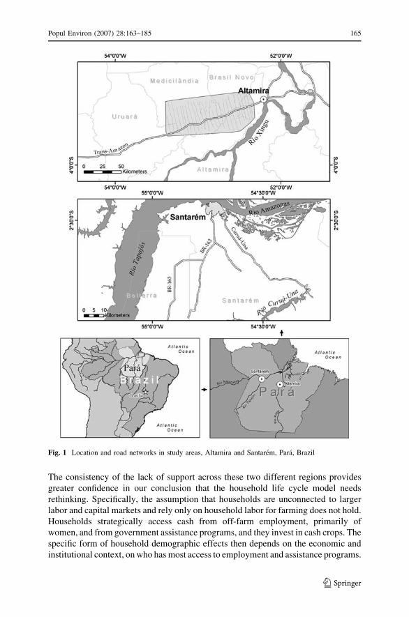
Fig. 1 Location and road networks in study areas, Altamira and Santarem, Para, Brazil

Popul Environ (2007) 28:163–185 165

123

Household demography and land use/land cover in frontiers

Research considering the effects of household demography on land use or land

cover in frontier regions, as our study areas are, has focused on the ‘‘household life

cycle.’’ The focus on the developmental cycle of the household is based in

anthropology (Goody, 1958), and arguments about the mechanisms (particularly the

demographic composition of the household) are based on the Chayanovian peasant

economy model (Chayanov, 1966; Walker et al., 2002, 2004; Walker & Homma,

1996). Walker (2003) and Walker and Homma (1996) develop the theoretical

principles underlying the modeling of household demographic and other effects by

combining the Chayanovian approach with a household production model (and

recognizing the changing institutional context of the frontier). In its basic form, this

approach assumes that households have no access to capital or to hired labor, and

that households focus on production to meet consumption needs (rather than to

accumulate capital). When households enter a frontier, in which land is abundant

and labor and capital are scarce, their land use decisions are determined by

household demography. Household demography influences the decisions in three

ways.

First, it represents the consumption needs of the household. In Chayanov’s

original formulation, peasants exist outside of a monetary or exchange economy and

therefore produce primarily to meet consumption needs. This argues for a positive

effect of children and elderly dependents, and of household size on the extent of

land used. Second, household demography determines the amount of labor available

for farming which, in the absence of capital and labor-saving technology,

determines the amount of land that can be used. This argues for a positive effect

of the number of working age members of the household, particularly males in a

setting where men do the majority of the farm work, on the extent of land used.

Third, as the owners of land and their children age and as their children move to

other properties or to urban areas, the time horizon of the owners changes.

Households with many small children have a short time horizon, seeing only the

need to feed and care for the family for the next few years. As these children

become able to help with farm work, and available labor increases beyond the

minimum necessary to support the family, households begin to make investments in

perennial crops or pasture. These are activities that require many years of

investment before generating a return, but which provide a higher return (depending

on market conditions) and/or can be managed with less labor in the long run. While

some have argued for using the age of the household head as an additional covariate

in models to test the role of aging, the theoretical basis of the changes seen over

time in empirical analyses is the changing demographic composition of the

household.

This approach has been used by many researchers studying household land use

decision-making in the Brazilian and Ecuadorian Amazon (Brondızio et al., 2002;

Futemma & Brondızio, 2003; McCracken et al., 1999, 2002; Moran, Brondızio, &

McCracken, 2002; Pan et al., 2001, 2004; Perz, 2001; Perz & Walker, 2002; Pichon,

1996b; Walker et al., 2002). Walker, Perz and colleagues have used this approach in

their study area around Uruara in the state of Para in the Brazilian Amazon (located

166 Popul Environ (2007) 28:163–185

123

between our two study areas). Based on their own analyses and on an extensive

review of the literature, they find mixed evidence for household life cycle effects

using a variety of data and methods. Walker et al. (2002) review the extensive

relevant literature, which shows mixed effects of household demographic compo-

sition on land use. Measures of age of the household head, age of the head at arrival

in the property, family size, and the numbers of adult males, females and children

have generally non-significant effects on a variety of outcomes used by other

researchers, including areas or percent of property in annuals, perennials, pasture

and forest, area deforested, and a variety of measures of production.

Walker et al. (2002) also conduct an empirical analysis of the effects of

household demographic characteristics on farm system (combination of land uses)

using survey data for a sample of farm households. Results show that the

dependency ratio (ratio of consumers to producers) and male family workers each

significantly predict only one of six farming systems. These effects are consistent

with the theoretical approach, as the number of male family members has a positive

effect on the probability of growing ‘‘annuals with perennials’’ and the dependency

ratio has a negative effect on the probability of growing ‘‘perennials with annuals.’’

However, the evidence is not overwhelming for these demographic effects. The

number of men in the household and the dependency ratio generally have non-

significant effects on farm system. The age of the household head has no significant

effect in any of their models. Using the same approach and the same data, Perz

(2001) finds that the number of adults in the household (undifferentiated by gender)

has a positive effect on the area in perennials and pasture and on cattle production.

The number of children has no significant effect in these models.

McCracken, Brondızio and colleagues have also used a household life cycle

approach in their study area in Altamira, one of the areas included in our analyses in

this paper (Brondızio et al., 2002; McCracken et al., 1999, 2002). This research used

remotely sensed measures of forest cover, and also used the time since settlement

(opening of a property) as a proxy for household life cycle. The authors find

evidence of changing deforestation rates (based on remotely sensed data) over the

household life cycle (Brondızio et al., 2002; McCracken et al., 1999), with initially

low rates of deforestation after settlement, followed by a peak in deforestation

within 3–5 years after settlement and another peak 10–15 years after settlement

(Brondızio et al., 2002). However, they use the time since settlement as a proxy for

the life cycle stage of the household. They use a cohort-based approach, examining

each settlement cohort separately and finding the same over time pattern for each

but not exploring the mechanisms underlying that pattern. They also point out that

there is more variation within cohorts than across cohorts, reflecting differences in

household characteristics (including life cycle stage and household demography at

settlement).

Bilsborrow, Pichon and colleagues have examined household demographic or

household life cycle effects on land use among farm colonist households in the

Northern Ecuadorian Amazon. They initially used their field observations to argue

for a refinement of traditional models of rural livelihoods which assumed land

scarcity and labor abundance, the reverse of what is found in Amazonian frontiers

(Pichon, 1996b). In empirical analysis using survey data from their sample of farms

Popul Environ (2007) 28:163–185 167

123

in a Northern Ecuadorian Amazon settlement area, they find that women with

children under 12 are more likely to participate in farmwork (Thapa, Bilsborrow, &

Murphy, 1996). They also find that area in perennials and pasture increases as a

function of household size but that the area in food crops in not significantly related

to household size (Pichon, 1996a). They similarly find household life cycle effects

on forest clearing (Marquette, 1998). However, they find that no measures of

household size or composition significantly predict farm income, participation in

off-farm work or income from cattle (Murphy, 2001).

In more recent work, this team has both linked remotely sensed data to their

survey data and used generalized linear mixed models to estimate household and

community effects on land use / land cover (Pan et al., 2001, 2004; Pan &

Bilsborrow, 2005). This recent work uses the percent of area in a variety of land

covers or land uses (summing to 100% of the property) as dependent variables in

statistical models that simultaneously predict all of the outcomes (dealing with the

correlations between choices about, e.g., perennials and pasture). These models do

not show strong support for the household life cycle or household production

approaches, but they do show some of the expected effects of household labor

supply and children on area in annuals, perennials, pasture and forest (with slightly

different specifications of household demographic variables in each paper). For

example, models in Pan and Bilsborrow (2005) show a positive effect of males on

perennials and a negative effect of males on forest, while showing a negative effect

of children on perennials and a positive effect of children on annuals.

In many of these articles and other work by these research teams predicting

related outcomes, the time on the property has a significant effect on the farm

system or extent of various land uses. The authors largely interpret this as a

household life cycle effect. However, this assumes that only young families settle on

new properties. We and others argue that the effects of the time since arriving on the

property reflects a different sort of cycle. Barbieri, Bilsborrow, and Pan (2005)

argue for a property life cycle, in which land is cleared at different rates depending

on the duration of residence on a property. VanWey, Brondızio, D’Antona, and

Moran (2007) argue for a learning process, where new arrivals in frontiers must

clear large areas of land to experiment with different crops and inputs. Older

residents of new frontiers and newer residents of old frontiers (where agricultural

techniques and knowledge have diffused through the population) need not

experiment in this way and instead can specialize in crops appropriate for their land.

Overall, the empirical literature on the effects of household demography on land

use or land cover is mixed. While there are strong theoretical underpinnings for the

household life cycle model and for effects of household labor and dependents, the

empirical literature shows few significant effects in a large number of models with

varying specifications of independent variables. Further, the classic work in this area

has been challenged by the introduction of the property life cycle in place of the

household life cycle. The variable results could be due to variations across study

areas (as all are based on case studies) or across measurement of dependent

variables (particularly between remotely sensed and survey data), or to inconsistent

specification of independent variables. In particular, the focus of household life

cycle and household production models on household labor and dependents has led

168 Popul Environ (2007) 28:163–185

123

many past researchers to include only measures of the number of adults or adult

males, and number of children or dependency ratio, rather than decomposing the

household into all of its constituent age-gender groups. We endeavor to make a

more rigorous, though still limited, test of these household demographic effects by

specifying identical models, with household demography decomposed into all age-

gender groups and with dependent variables measured from both survey data and

remotely sensed data, for two study areas.

Study areas

Figure 1 shows the locations of our two study areas within the state of Para in Brazil

and the basic road and river networks in each study area. Altamira is a region of

rolling topography, including frequent steep slopes that are unsuitable for many

crops. It is characterized by relatively fertile soils and plenty of available water. The

main rural economic activities are cattle ranching and cocoa production, along with

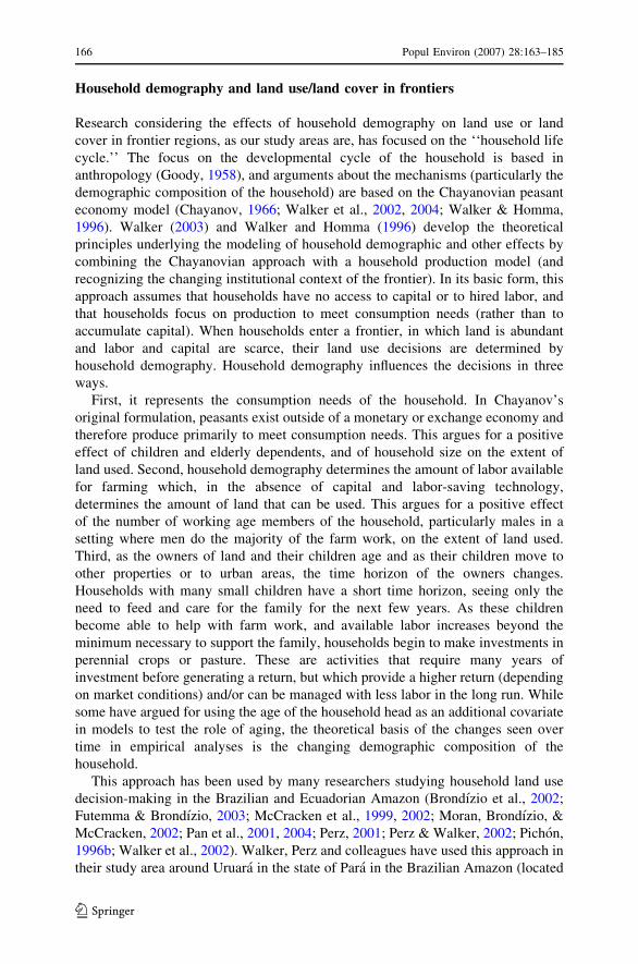
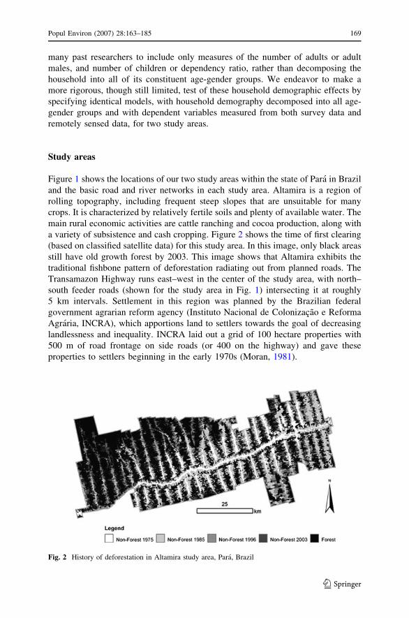
a variety of subsistence and cash cropping. Figure 2 shows the time of first clearing

(based on classified satellite data) for this study area. In this image, only black areas

still have old growth forest by 2003. This image shows that Altamira exhibits the

traditional fishbone pattern of deforestation radiating out from planned roads. The

Transamazon Highway runs east–west in the center of the study area, with north–

south feeder roads (shown for the study area in Fig. 1) intersecting it at roughly

5 km intervals. Settlement in this region was planned by the Brazilian federal

government agrarian reform agency (Instituto Nacional de Colonizacao e Reforma

Agraria, INCRA), which apportions land to settlers towards the goal of decreasing

landlessness and inequality. INCRA laid out a grid of 100 hectare properties with

500 m of road frontage on side roads (or 400 on the highway) and gave these

properties to settlers beginning in the early 1970s (Moran, 1981).

Fig. 2 History of deforestation in Altamira study area, Para, Brazil

Popul Environ (2007) 28:163–185 169

123

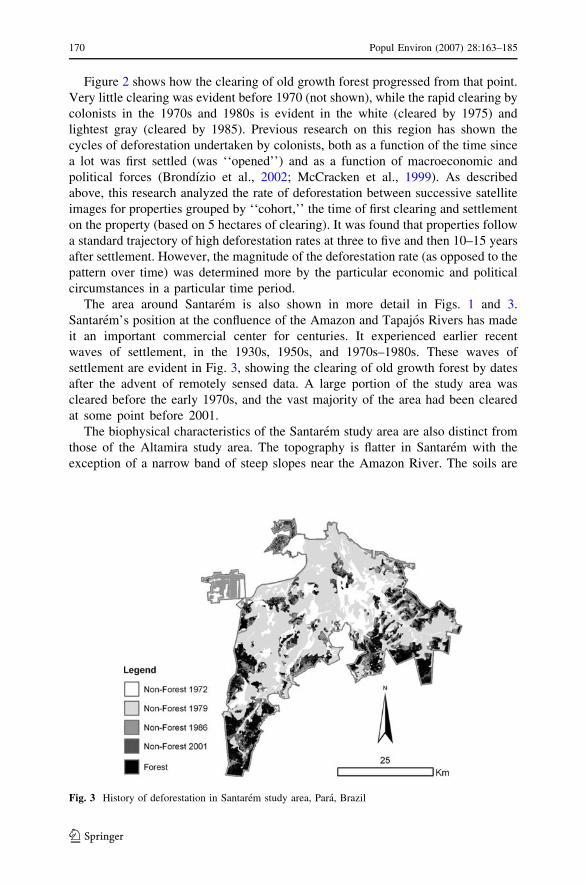
Figure 2 shows how the clearing of old growth forest progressed from that point.

Very little clearing was evident before 1970 (not shown), while the rapid clearing by

colonists in the 1970s and 1980s is evident in the white (cleared by 1975) and

lightest gray (cleared by 1985). Previous research on this region has shown the

cycles of deforestation undertaken by colonists, both as a function of the time since

a lot was first settled (was ‘‘opened’’) and as a function of macroeconomic and

political forces (Brondızio et al., 2002; McCracken et al., 1999). As described

above, this research analyzed the rate of deforestation between successive satellite

images for properties grouped by ‘‘cohort,’’ the time of first clearing and settlement

on the property (based on 5 hectares of clearing). It was found that properties follow

a standard trajectory of high deforestation rates at three to five and then 10–15 years

after settlement. However, the magnitude of the deforestation rate (as opposed to the

pattern over time) was determined more by the particular economic and political

circumstances in a particular time period.

The area around Santarem is also shown in more detail in Figs. 1 and 3.

Santarem’s position at the confluence of the Amazon and Tapajos Rivers has made

it an important commercial center for centuries. It experienced earlier recent

waves of settlement, in the 1930s, 1950s, and 1970s–1980s. These waves of

settlement are evident in Fig. 3, showing the clearing of old growth forest by dates

after the advent of remotely sensed data. A large portion of the study area was

cleared before the early 1970s, and the vast majority of the area had been cleared

at some point before 2001.

The biophysical characteristics of the Santarem study area are also distinct from

those of the Altamira study area. The topography is flatter in Santarem with the

exception of a narrow band of steep slopes near the Amazon River. The soils are

Fig. 3 History of deforestation in Santarem study area, Para, Brazil

170 Popul Environ (2007) 28:163–185

123

less fertile in Santarem, with a relative paucity of the fertile terra roxa (alfisols)

that is more common in Altamira. Santarem also experiences more frequent water

shortages. Wells must be deep and water is hard to come by. As a result, Altamira

is more suited to the raising of cattle and permits more effective production of

perennial crops. This is not to say that production of perennials is not possible in

Santarem, or that farmers cannot raise cattle, but respondent reports indicate that

both are harder. This tendency away from cattle production and perennials is

exacerbated by the recent introduction of soybeans into the Santarem area, with

the multinational Cargill constructing a deep water port on the Amazon River in

the city accompanied by land consolidation and large scale mechanized soy

production.

The differences in topography and settlement history between Altamira and

Santarem have led to more secondary growth and a more complex landscape in

Santarem. Despite the majority of the area having been cleared by the 1990s, there

is a lot more secondary growth evident in satellite images of Santarem (not shown).

This reflects the lower prevalence of pasture and the larger proportion of the area in

some sort of secondary growth (from small scrubby growth to areas that are

indistinguishable from forest in satellite imagery). The higher level of complexity in

the landscape includes clearing following both road networks and river networks

and a preponderance of small, irregularly shaped properties. This reflects the longer

and unplanned settlement history of Santarem.

Data and measures

The samples for the social survey data collection are based on INCRA property

grids for each study area. In Altamira, the grid represents the settlement plan for the

region, while in Santarem the grid is for planned settlement in a small portion of the

region and is a regularization of existing land tenure in the remainder of the region.

In Altamira, we selected a stratified random sample of properties from the property

grid. Each property in the grid was assigned to a settlement cohort, based on the

year in which a cleared area of 5 hectares was visible in a satellite image. Within

each cohort, we then selected a random sample of properties, with the goal of an

equal representation of cohorts in the final sample, despite the larger number of

properties in the earlier cohorts in the population.

We visited each of these properties in either 1997 or 1998 and interviewed the

household of the property owner, conducting interviews usually with the male and

female heads of household about land use and production and about household

demography and economy, respectively. In some cases, we substituted an alternate

property for the originally sampled property when the sampled property was vacant

or the owners were impossible to locate to interview.1 The interview with the male

head of household included information on the various land uses on the property at

the time of acquisition and at the time of the survey, and included a land use history

1 Sampled properties were not replaced with alternates because of owners refusing to participate. In this

wave of data collection we had no farmers refuse to participate in our study.

Popul Environ (2007) 28:163–185 171

123

showing the changes in area in certain land uses over the ownership of the property.

The conversations about current and past land use were facilitated by sketch maps

that the interviewers drew with the farmers and by satellite images from four dates

showing the property, which the interviewers interpreted with the farmer. This

information allows us to estimate the area in various uses in any year that the

household owned the property. The interview with the female head of household

included information about the current and past composition of the household,

allowing us to construct measures of the household size and composition in any year

since the household arrived on the property. All of the properties in this sample

(subject to some restrictions described below) are included in our analyses for this

paper.

In Santarem, we also sampled from an existing property grid with the goal of an

equal representation of properties occupied at different times. Because of the longer

settlement history, we were not able to stratify the population of properties in the

study area by time of first clearing. Instead, we stratified by region within the study

area. Each region follows a major road—from West to East, the Cuiaba-Santarem

Highway (BR-163), smaller roads to Jabutı and Mojuı dos Campos, and the Curua-

Una Highway—which was opened in a different era, leading to settlement of the

region at a different time. Within each region, we overlaid a grid of 3 km by 3 km

cells and selected a sample of these cells to achieve a spatially clustered sample to

reduce transportation costs. Within each of these cells, we selected five target

properties and four alternates (or fewer if there were fewer than nine properties in

the cell).

We visited these target properties in the summer of 2003 and attempted to

interview both the household of the owner of the property and any other households

on the property. Because of the long settlement history and a more active land

market in Santarem, we encountered three situations that made the achievement of

interviews in all sampled properties difficult. First, many properties had been

divided and the area covered by the sampled property was occupied by multiple

properties or by parts of multiple properties. In this case, we attempted to interview

all the properties that were wholly or partially in the area covered by the sampled

property. Second, many other properties had been aggregated with others into large

farms, often managed by absentee owners or used for commercial farming with no

households resident onsite. In this case, we interviewed the owning household if that

household lived on some portion of the aggregated land and managed it themselves.

If the farm owner was absent and/or the farm was managed completely as a

commercial endeavor, we collected a limited set of data about the current owner and

land use transformations on the property from neighbors and workers. Third, we

encountered areas in which the property grid bore no resemblance to the actual

division of land and no informants could remember a time in which land had been

partitioned in that way. In this case, we again attempted to conduct interviews in all

properties wholly or partially in the area covered by the sampled property. For the

analysis below, we restrict the sample to the households of property owners on the

properties that are still owned and managed as family properties (as opposed to as

commercial farms).

172 Popul Environ (2007) 28:163–185

123

In both study areas, we further restrict our sample in three ways for the analyses

for this paper. First, we include only households who have owned their properties

for approximately 10 years prior to the survey. The exact dates of ownership differ

between study areas because of different availability of remotely sensed data. We

use images from 1988, 1991, and 1996 for Altamira and from 1991 and 2001 for

Santarem. We use survey data from 1986 through 1996 for Altamira and from 1989

through 2001 for Santarem, giving us 2 years of data for measuring household

characteristics prior to the first image. We limit the sample to households who have

owned their properties in all these years. Second, we limit the sample to properties

that have less than 10% cloud or cloud shadow in each of the remotely sensed

images. This limitation reduces the error in the land use measure based on the

satellite data, as the area in forest calculated from the satellite data is based only on

the observable part of the property (i.e., the part without clouds). Third, we limit the

sample to properties that are larger than 5 hectares (a size that precludes even

subsistence farming over the long term). This is only a consideration in Santarem as

all of the properties in Altamira are substantially larger than that.

We create five dependent variables (in each study area) from the survey and

satellite data for the analyses for this paper. First, we measure the area planted in

annuals in a given year. This value is measured directly in a land use history

collected from respondents. Second, we measure the area in pasture in a given year

by beginning with the area in pasture when the property was acquired, adding

pasture area added over time (reported in the land use history), and subtracting

pasture allowed to go fallow over time (reported in the land use history). Third, we

measure perennials using the same procedure as pasture, beginning with the area in

perennials when the property was acquired and adding or subtracting areas reported

in the land use history. Fourth, we create measures of the area on the property in

forest from the survey data. The area in forest is calculated as the area in forest

when the household acquired the property minus any areas that have been cleared

between arrival and a given year. While these variables covary to a certain extent, in

the sense that a property cannot be 100% forest and 100% crops, they do not exactly

covary nor do they sum to property size as many properties have substantial areas in

fallow and all properties have some areas used for houses and yards, roads, and/or

water.

Fifth, we use one measure of land cover based on remotely sensed data. This

measures the area in a property that is in forest. The satellite images are all Landsat

images, taken in July of 1988 and 1991, and June of 1996 over the Altamira study

area and in July of 1991 and 2001 over the Santarem study area. We used a

combination of supervised and unsupervised classification techniques to classify

each pixel in these images into a specific land cover (or into cloud or cloud shadow).

These classifications produced a continuous surface of land cover for each study

area for each time point. We then partitioned the portion of the landscape associated

with each surveyed property using the boundaries of the property in the property

grid (Evans, VanWey, & Moran, 2005). These boundaries were updated during

fieldwork based on the information provided by farmers and on GPS (global

positioning system) points taken at the corners of properties.

Popul Environ (2007) 28:163–185 173

123

The classification we completed includes the following categories: forest,

secondary succession 3 (SS3), secondary succession 2 (SS2), secondary succession

1 (SS1), bare, pasture, water, cloud, and cloud shadow for Altamira (Moran et al.,

2002; Tucker, Brondızio, & Moran, 1998);2 forest (two types), forest/SS3, SS2/SS3,

SS2, SS1/SS2, SS1, bare/SS1, bare, cloud, and cloud shadow for the first Santarem

image; and bare (divided into high and low reflectance), agriculture, pasture, SS1,

SS2, forest, and water for the second image from Santarem.3 Because these

categories are based on ecological considerations, including the amount of

vegetation and the relative amounts of herbaceous and woody vegetation, making

measures that are comparable to the survey-based measures is difficult. The most

comparable measure is the measure of forest, and we include that measure here. We

use only forested area as a satellite-based dependent variable primarily as a test for

the sensitivity of our survey-based results to alternative measures. The measure of

forest cover in the analyses below uses the area classified as forest or SS3 in

Altamira and the area classified as forest or forest/SS3 in Santarem. SS3 is not old

growth forest, but it is densely vegetated area that can be considered similar to old

growth forest (evidenced by our inability to distinguish SS3 from forest in our

Santarem classification). We create a measure of the area in the property that is

forested in each year for which satellite data are available.

Our independent variables include the composition of the household and dummy

variables to capture period effects. Because we are using fixed effects models (see

below for model description), all time invariant household or property character-

istics are controlled, including such things as the area of the property, the age of the

householder when he acquired the property, the location of the property, etc. Thus,

our models examine only the effects of time varying household characteristics, in

this case household composition. We measure the household demographic

composition in two ways in any given year. We first create count variables

showing the number of household members in the following categories: children

(ages 0–11), female adolescents (ages 12–18), male adolescents (ages 12–18),

female adults (ages 19–49), male adults (ages 19–49), older females (ages 50+) and

older males (ages 50+). These numbers are created by taking the demographic

composition of the household at the time of the survey, removing any current

members who were not yet in the household in the year (for example, children who

had yet to be born), adding any past members who had left by the time of the survey

(for example, children who were in the household but had left by the time of the

survey), and then computing the number of members in each sex-age group from the

sexes and dates of birth of all of the members. To reduce the effect of errors in the

recall of the exact timing of events and to reflect the possible lag time between

household demographic change and land use change, these counts are averaged over

2 SS3 is the most advanced secondary growth, while SS1 is the least. In 1991, the classification also

included a category for sugar cane, capturing a short-lived explosion of sugar cane cultivation during the

operation of a factory for converting sugar cane to alcohol. These areas were subsequently abandoned or

converted to other uses, primarily cocoa. We do not use this category in our analyses.3 The differences among the classifications reflect both differences in the ability of the research team to

distinguish categories and differences in the initial uses of the classified imagery.

174 Popul Environ (2007) 28:163–185

123

the three years leading up to the measurement of the dependent variable (e.g., 1986,

1987, and 1988 for observations in 1988).

We tested two other measurements of household composition in our models. We

created dummy variables for groups of values for each of the groups (e.g., zero

children, 1 child, two children, etc.), based on the counts averaged over the 3 years

leading up to the target year. For example, if the value of the count of children was

1.33, we assigned that household to be 1 on a dummy measuring whether there was

1 child in the household, while if the value was 1.67 we assigned the household to

be a 1 on a dummy measuring 2 or 3 children in the household (2 or 3 because so

few households had exactly 2 or exactly 3). We then created dummy variables

indicating whether or not there was a household member in each age-gender group.

We created these measures by assigning the household a value of 1 on the dummy if

the household had any members in the age-gender group in at least 2 of the 3 years

leading up to the target year. In comparisons between models, the models using the

count measures or the dummies indicating any member in the age-gender group

outperformed the models with the dummies for different numbers of members

within each age-gender group. Thus, the models shown in Tables 2 and 3 include

some models with the count measures and some with the dummies, depending on

which performed better according to model comparisons using the Bayesian

Information Criterion (Raftery, 1995) and the Akaike Information Criterion (Judge,

Griffiths, Hill, Lutkepohl, & Lee, 1985).

These measures allow us to distinguish between the effects of dependents

(children and older members) and prime working age household members, and

allow us to examine the gendered nature of demographic effects. The household life

cycle or household production approach argues for increases in production as a

function of dependents and as a function of members who are able to contribute

labor to production. Because of the nature of farming in these regions, the majority

of the labor is supplied by men, suggesting that the number of females, children and

older members should have a positive effect on production (given their role as

consumers), but that the number of working age males should have a stronger effect

(Siqueira, McCracken, Brondızio, & Moran, 2003).

The descriptive statistics on the dependent and independent variables for the two

analysis samples (for Altamira and for Santarem) are shown in Table 1. Differences

in the areas in various uses in the average household-year in the two study areas

reflect differences in property size, history, and major economic activities. In both

areas, households plant an average of around 3 hectares of annuals each year,

reflecting the amount needed for subsistence. In Altamira, however, households also

have an average of 34 hectares of pasture and 10 hectares of perennials in the

average household-year. This reflects the economic base of the region, with most

families producing for the market and the biophysical conditions being appropriate

for cattle raising and perennials (mostly cocoa). The average areas in forest based on

the two measurements (survey and satellite) show the recent occupation of Altamira

and the smaller average property size in Santarem (34.61 hectares versus an average

of 110.64 in Altamira). Properties in Altamira were settled sometime between the

early 1970’s and the mid 1990’s, meaning that many properties still have a large

area of relatively undisturbed forest. Properties in Santarem were settled over the

Popul Environ (2007) 28:163–185 175

123

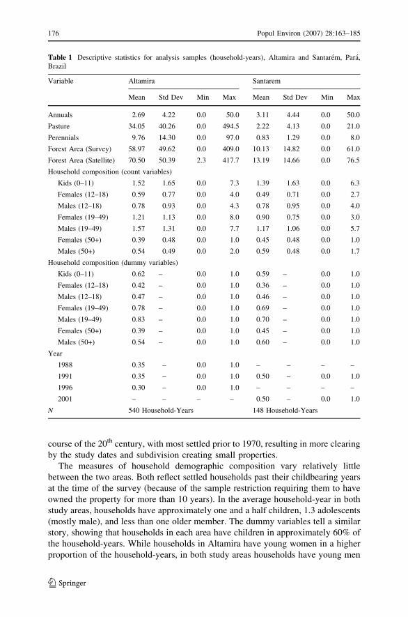
course of the 20th century, with most settled prior to 1970, resulting in more clearing

by the study dates and subdivision creating small properties.

The measures of household demographic composition vary relatively little

between the two areas. Both reflect settled households past their childbearing years

at the time of the survey (because of the sample restriction requiring them to have

owned the property for more than 10 years). In the average household-year in both

study areas, households have approximately one and a half children, 1.3 adolescents

(mostly male), and less than one older member. The dummy variables tell a similar

story, showing that households in each area have children in approximately 60% of

the household-years. While households in Altamira have young women in a higher

proportion of the household-years, in both study areas households have young men

Table 1 Descriptive statistics for analysis samples (household-years), Altamira and Santarem, Para,

Brazil

Variable Altamira Santarem

Mean Std Dev Min Max Mean Std Dev Min Max

Annuals 2.69 4.22 0.0 50.0 3.11 4.44 0.0 50.0

Pasture 34.05 40.26 0.0 494.5 2.22 4.13 0.0 21.0

Perennials 9.76 14.30 0.0 97.0 0.83 1.29 0.0 8.0

Forest Area (Survey) 58.97 49.62 0.0 409.0 10.13 14.82 0.0 61.0

Forest Area (Satellite) 70.50 50.39 2.3 417.7 13.19 14.66 0.0 76.5

Household composition (count variables)

Kids (0–11) 1.52 1.65 0.0 7.3 1.39 1.63 0.0 6.3

Females (12–18) 0.59 0.77 0.0 4.0 0.49 0.71 0.0 2.7

Males (12–18) 0.78 0.93 0.0 4.3 0.78 0.95 0.0 4.0

Females (19–49) 1.21 1.13 0.0 8.0 0.90 0.75 0.0 3.0

Males (19–49) 1.57 1.31 0.0 7.7 1.17 1.06 0.0 5.7

Females (50+) 0.39 0.48 0.0 1.0 0.45 0.48 0.0 1.0

Males (50+) 0.54 0.49 0.0 2.0 0.59 0.48 0.0 1.7

Household composition (dummy variables)

Kids (0–11) 0.62 – 0.0 1.0 0.59 – 0.0 1.0

Females (12–18) 0.42 – 0.0 1.0 0.36 – 0.0 1.0

Males (12–18) 0.47 – 0.0 1.0 0.46 – 0.0 1.0

Females (19–49) 0.78 – 0.0 1.0 0.69 – 0.0 1.0

Males (19–49) 0.83 – 0.0 1.0 0.70 – 0.0 1.0

Females (50+) 0.39 – 0.0 1.0 0.45 – 0.0 1.0

Males (50+) 0.54 – 0.0 1.0 0.60 – 0.0 1.0

Year

1988 0.35 – 0.0 1.0 – – – –

1991 0.35 – 0.0 1.0 0.50 – 0.0 1.0

1996 0.30 – 0.0 1.0 – – – –

2001 – – – – 0.50 – 0.0 1.0

N 540 Household-Years 148 Household-Years

176 Popul Environ (2007) 28:163–185

123

in more years (46–47% of years) than they have young women (36% or 42% of

years). The proportions of years with older members almost exactly match the

average number of older members, because households who have older men or

women tend to have only one of each.

Households in Altamira tend to have more prime working age members, with 1.2

such women and 1.6 such men. Households in Santarem have less than one 19–

49 year old man and 1.2 such women in the average household-year. These

tendencies are again mirrored in the dummy variables. In Altamira, households have

prime working age women in 78% of years and prime working age men in 83% of

years. In Santarem, reflecting the older settlement there (and therefore slightly

greater representation of older households), households have prime working age

women in 69% of years and prime working age men in 70% of years.

Analytic strategy

To estimate the effects of changing household composition on changes in land use,

we employ fixed effects linear regression models. These models can be estimated

using a variety of technical procedures with the same results.4 Intuitively, we can

think of a fixed effects model as estimating the effects of changes in independent

variables on changes in dependent variables, holding constant the effects of any

time-invariant (observed or unobserved) characteristics of the cases. Intuitively we

can think of the following equation for the case of two observations of each case:

Yi2 � Yi1ð Þ ¼ b02 � b01ð Þ þ b1 Xi2 � Xi1ð Þ þ b2 Zi � Zið Þ þ e2 � e1ð Þ

where the left hand side is the change in the dependent variable for case i between

time 1 and time 2. This change is a function of the change in the intercept terms, the

effect of the change in the time-varying independent variables (X) and an error term.

The third term reduces to zero because the time-invariant characteristics of the cases

(Z) are the same at time 1 and time 2. In our models we estimate the effects of

changes in household composition (the X variables) on changes in land use (the Yvariables), holding constant such time-invariant characteristics as initial conditions

on the property, time of settlement, risk aversion, past experience with various

crops, and property size (the Z variables).

In order for these models to effectively estimate the effects of changing

household composition on changes in land use, two conditions must be met. We

must include multiple observations for each household and the household

composition must vary over time within households. In each of our analysis

samples, we include at least two observations for each household (see sample

4 For ease of analysis, we use the xtreg, fe command in Stata. We replicated the results using two other

methods: using OLS regressions with dummy variables for all households and using OLS regressions of

deviations in a given dependent variable from the household mean on deviations in the independent

variables from their household means. These methods all produced the same coefficient estimates for the

effects of household composition, though the OLS using deviations method produced smaller standard

errors because it did not account for the degrees of freedom lost because of the household fixed effects.

Popul Environ (2007) 28:163–185 177

123

selection description above). In tables available upon request from the authors, we

show that there is variation in the measures of household composition over time.

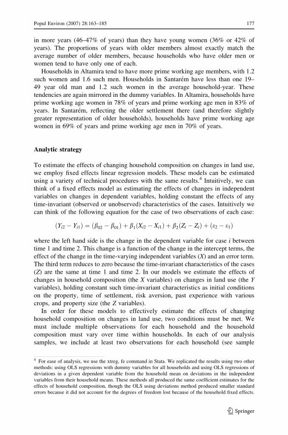
Results

Table 2 shows the fixed effects linear regression models for the Altamira sample.

Each model controls for time period, to account for secular changes in forest cover

and macro level period effects (e.g., credit programs and economic conditions).

Models of the area on the property in perennials and in forest (using satellite-based

measures) estimate the effects of change from no members to any members of each

age-gender group in the household. The models of area in annuals, pasture, and

forest (using survey-based measures) estimate the effects of changes in the number

of household members in each age-gender group.5 These models show few

significant effects of changes in household composition on land use change. Those

effects that are significant do not correspond to expectations based on household life

cycle or household production theories. Increases in the number of children (or

changes from no children to some children) increase the amount of pasture and

decrease the area in perennials, instead of increasing the area in annuals as predicted

by these theories.

Even more unexpected, the significant effects of adolescents, adults and older

household members are all effects of female household members. Adding female

adolescents (either through in-migration or children aging into adolescence)

significantly decreases forested area and has a marginally significant positive effect

on area in pasture. The household life cycle model argues that when children move

into adolescence, the household becomes able to plan for the future and therefore

will invest in land uses with a longer time until return (i.e., pasture and perennials).

However, the key adolescents for this increase in pasture and perennials should be

male adolescents, who provide much of the farm labor. Older women (50+) also

have significant effects on land use, negatively affecting both perennials and forest

(though only with the satellite-based measure of forest). Again following the

household life cycle and household production approaches, these older women

should affect only the household’s consumption needs and therefore primarily the

area in annuals. While older households are expected to be reducing their planted

area, it should be the transition of men rather than women out of prime working ages

that precipitates the change.

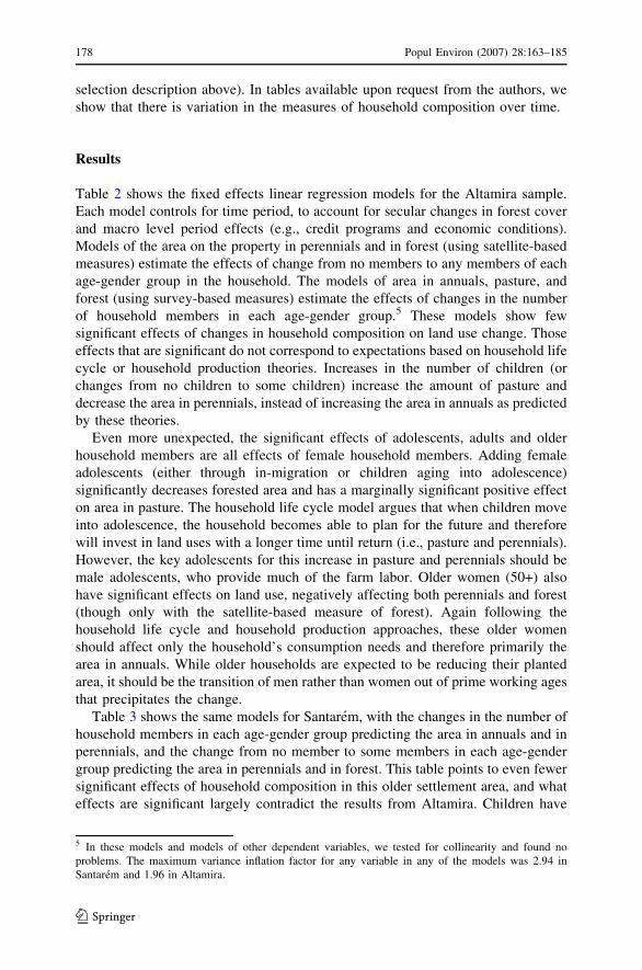
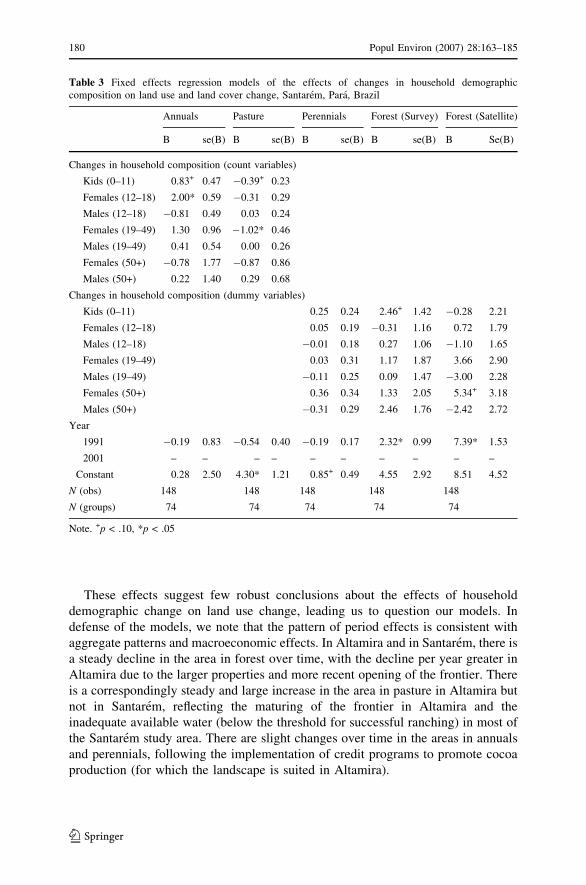
Table 3 shows the same models for Santarem, with the changes in the number of

household members in each age-gender group predicting the area in annuals and in

perennials, and the change from no member to some members in each age-gender

group predicting the area in perennials and in forest. This table points to even fewer

significant effects of household composition in this older settlement area, and what

effects are significant largely contradict the results from Altamira. Children have

5 In these models and models of other dependent variables, we tested for collinearity and found no

problems. The maximum variance inflation factor for any variable in any of the models was 2.94 in

Santarem and 1.96 in Altamira.

178 Popul Environ (2007) 28:163–185

123

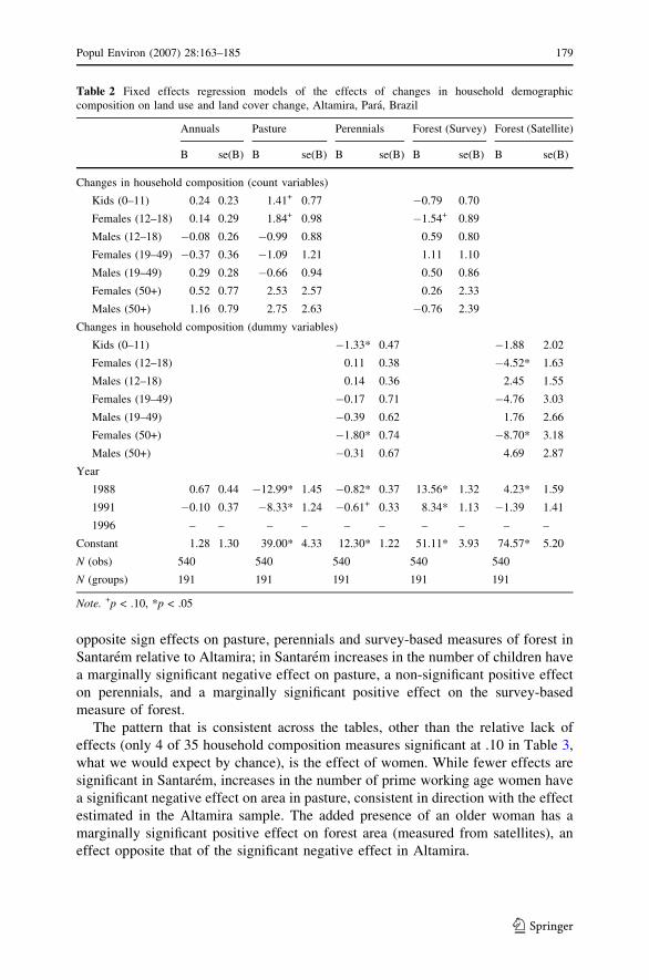
opposite sign effects on pasture, perennials and survey-based measures of forest in

Santarem relative to Altamira; in Santarem increases in the number of children have

a marginally significant negative effect on pasture, a non-significant positive effect

on perennials, and a marginally significant positive effect on the survey-based

measure of forest.

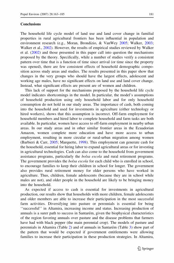
The pattern that is consistent across the tables, other than the relative lack of

effects (only 4 of 35 household composition measures significant at .10 in Table 3,

what we would expect by chance), is the effect of women. While fewer effects are

significant in Santarem, increases in the number of prime working age women have

a significant negative effect on area in pasture, consistent in direction with the effect

estimated in the Altamira sample. The added presence of an older woman has a

marginally significant positive effect on forest area (measured from satellites), an

effect opposite that of the significant negative effect in Altamira.

Table 2 Fixed effects regression models of the effects of changes in household demographic

composition on land use and land cover change, Altamira, Para, Brazil

Annuals Pasture Perennials Forest (Survey) Forest (Satellite)

B se(B) B se(B) B se(B) B se(B) B se(B)

Changes in household composition (count variables)

Kids (0–11) 0.24 0.23 1.41+ 0.77 �0.79 0.70

Females (12–18) 0.14 0.29 1.84+ 0.98 �1.54+ 0.89

Males (12–18) �0.08 0.26 �0.99 0.88 0.59 0.80

Females (19–49) �0.37 0.36 �1.09 1.21 1.11 1.10

Males (19–49) 0.29 0.28 �0.66 0.94 0.50 0.86

Females (50+) 0.52 0.77 2.53 2.57 0.26 2.33

Males (50+) 1.16 0.79 2.75 2.63 �0.76 2.39

Changes in household composition (dummy variables)

Kids (0–11) �1.33* 0.47 �1.88 2.02

Females (12–18) 0.11 0.38 �4.52* 1.63

Males (12–18) 0.14 0.36 2.45 1.55

Females (19–49) �0.17 0.71 �4.76 3.03

Males (19–49) �0.39 0.62 1.76 2.66

Females (50+) �1.80* 0.74 �8.70* 3.18

Males (50+) �0.31 0.67 4.69 2.87

Year

1988 0.67 0.44 �12.99* 1.45 �0.82* 0.37 13.56* 1.32 4.23* 1.59

1991 �0.10 0.37 �8.33* 1.24 �0.61+ 0.33 8.34* 1.13 �1.39 1.41

1996 – – – – – – – – – –

Constant 1.28 1.30 39.00* 4.33 12.30* 1.22 51.11* 3.93 74.57* 5.20

N (obs) 540 540 540 540 540

N (groups) 191 191 191 191 191

Note. +p < .10, *p < .05

Popul Environ (2007) 28:163–185 179

123

These effects suggest few robust conclusions about the effects of household

demographic change on land use change, leading us to question our models. In

defense of the models, we note that the pattern of period effects is consistent with

aggregate patterns and macroeconomic effects. In Altamira and in Santarem, there is

a steady decline in the area in forest over time, with the decline per year greater in

Altamira due to the larger properties and more recent opening of the frontier. There

is a correspondingly steady and large increase in the area in pasture in Altamira but

not in Santarem, reflecting the maturing of the frontier in Altamira and the

inadequate available water (below the threshold for successful ranching) in most of

the Santarem study area. There are slight changes over time in the areas in annuals

and perennials, following the implementation of credit programs to promote cocoa

production (for which the landscape is suited in Altamira).

Table 3 Fixed effects regression models of the effects of changes in household demographic

composition on land use and land cover change, Santarem, Para, Brazil

Annuals Pasture Perennials Forest (Survey) Forest (Satellite)

B se(B) B se(B) B se(B) B se(B) B Se(B)

Changes in household composition (count variables)

Kids (0–11) 0.83+ 0.47 �0.39+ 0.23

Females (12–18) 2.00* 0.59 �0.31 0.29

Males (12–18) �0.81 0.49 0.03 0.24

Females (19–49) 1.30 0.96 �1.02* 0.46

Males (19–49) 0.41 0.54 0.00 0.26

Females (50+) �0.78 1.77 �0.87 0.86

Males (50+) 0.22 1.40 0.29 0.68

Changes in household composition (dummy variables)

Kids (0–11) 0.25 0.24 2.46+ 1.42 �0.28 2.21

Females (12–18) 0.05 0.19 �0.31 1.16 0.72 1.79

Males (12–18) �0.01 0.18 0.27 1.06 �1.10 1.65

Females (19–49) 0.03 0.31 1.17 1.87 3.66 2.90

Males (19–49) �0.11 0.25 0.09 1.47 �3.00 2.28

Females (50+) 0.36 0.34 1.33 2.05 5.34+ 3.18

Males (50+) �0.31 0.29 2.46 1.76 �2.42 2.72

Year

1991 �0.19 0.83 �0.54 0.40 �0.19 0.17 2.32* 0.99 7.39* 1.53

2001 – – – – – – – – – –

Constant 0.28 2.50 4.30* 1.21 0.85+ 0.49 4.55 2.92 8.51 4.52

N (obs) 148 148 148 148 148

N (groups) 74 74 74 74 74

Note. +p < .10, *p < .05

180 Popul Environ (2007) 28:163–185

123

Conclusions

The household life cycle model of land use and land cover change in familial

properties in rural agricultural frontiers has been influential in population and

environment research (e.g., Moran, Brondızio, & VanWey 2005; Walker, 2003;

Walker et al., 2002). However, the results of empirical studies reviewed by Walker

et al. (2002) and those presented in this paper call into question the mechanisms

proposed by the theory. Specifically, while a number of studies verify a consistent

pattern over time that is a function of time since arrival (or time since the property

was opened), there are few consistent effects of household demographic compo-

sition across study areas and studies. The results presented in this paper show that

changes in the very groups who should have the largest effects, adolescent and

working age males, have no significant effects on land use and land cover change.

Instead, what significant effects are present are of women and children.

This lack of support for the mechanisms proposed by the household life cycle

model indicates shortcomings in the model. In particular, the model’s assumptions

of household production using only household labor and for only household

consumption do not hold in our study areas. The importance of cash, both coming

into the household and used for investments in agriculture (either technology or

hired workers), shows that this assumption is incorrect. Off-farm employment for

household members and hired labor to complete household and farm tasks are both

available. In particular, women have access to off-farm employment in nearby urban

areas. In our study areas and in other similar frontier areas in the Ecuadorian

Amazon, women complete more education and have more access to urban

employment, resulting in more circular or rural-urban migration among women

(Barbieri & Carr, 2005; Marquette, 1998). This employment can generate cash for

the household, essential for hiring labor to expand agricultural areas or for investing

in agricultural technologies. Cash can also come to the household from government

assistance programs, particularly the bolsa escola and rural retirement programs.

The government provides the bolsa escola for each child who is enrolled in school,

to encourage families to keep their children in school for longer. The government

also provides rural retirement money for older persons who have worked in

agriculture. Thus, children, female adolescents (because they are in school while

males are not), and older people in the household are likely to be bringing money

into the household.

As expected if access to cash is essential for investments in agricultural

production, our results show that households with more children, female adolescents

and older members are able to increase their participation in the most successful

farm activities. Diversifying into pasture or perennials is essential for being

‘‘successful’’ in Altamira, increasing income and status. Increasing production of

annuals is a surer path to success in Santarem, given the biophysical characteristics

of the region favoring annuals over pasture and the disease problems that farmers

have had with black pepper (the main perennial crop). The models of pasture and

perennials in Altamira (Table 2) and of annuals in Santarem (Table 3) show part of

the pattern that would be expected if government entitlements were allowing

families to increase their participation in these production strategies. In Altamira,

Popul Environ (2007) 28:163–185 181

123

increasing the number (as opposed to the presence) of children and female

adolescents increases the area in pasture. In Santarem, increasing the number of

children and female adolescents increases the area in annuals. The expected results

are not present in the model of perennials in Altamira, possibly because the usual

way of increasing production in perennials is the use of sharecroppers or permanent

workers rather than hired temporary laborers.

These models contrast with interpretations of past research showing a cyclical

pattern of deforestation at the household-farm property level. The strongest

predictor in past research has been the time since the property was first settled,

which has been interpreted as a household life cycle effect. Barbieri et al. (2005)

interpret this as a property life cycle effect, showing the process of clearing that

happens over time on a previously completely forested property as it is converted to

agropastoral production. In other work, we argue that this cycle represents a process

of settlers learning the appropriate uses of the land in a new frontier (VanWey et al.,

2007). The results presented here cannot speak to the exact reasons for the cyclical

pattern found in previous research. However, they add to this growing body of work

by showing that mechanisms proposed by the household life cycle model do not

explain the pattern. Specifically, they call into question the Chayanovian assumption

of a closed household without connection to labor or capital markets.

The pattern of results and the differences between study areas are also subject to

social and environmental contextual effects that we can not estimate in our models.

We speculate that government programs provide access to cash for households. Yet,

the bolsa escola program began nationwide in the late 1990s and early 2000s. Thus,

our analyses in Altamira do not include a time with this program, while our analyses

in Santarem include the beginning of this program. However, older persons (both

men and women) are covered by rural retirement programs throughout the period

under study. Similarly, the importance of women and their earning power is not

constant over time. It is characteristic of a particular period in the development of

the rural-urban linked system in the Amazon. It is likely that the future will bring

more widespread urban opportunities and therefore more access to cash employ-

ment for men. The environmental differences between our study areas determine in

part how (or if) the cash is invested in agriculture. We argue that cash is invested in

pasture in Altamira and annuals in Santarem because of differences in the suitability

of the land (and related differences in the development of agricultural markets). The

effects of these differences are themselves likely to be contextually determined. For

example, the suitability of Santarem for mechanized row crops is leading to an

expansion of large-scale soy production which may displace all small farming from

the region. It will increase available off-farm employment for all household

members but decrease the area of non-consumption crops for rural residents.

This paper therefore argues for a more nuanced view of both contextual effects

and household strategies. Economic and institutional context determine the effects

of household demography on land use and land cover change. Rather than either in-

migration to the frontier or expansion of economic opportunities in regional cities

representing a steamroller of change that inevitably leads to deforestation by

smallholder farmers, household demography interacts with the development of labor

markets and government programs to determine land use on a given farm.

182 Popul Environ (2007) 28:163–185

123

Households act strategically to access cash (from employment or from government

assistance) and then to invest it in non-subsistence land uses. This suggests several

possible pathways to intensification of agriculture in frontiers in the future as a

result of possible economic and institutional forces. First, the expansion of

government transfer programs could lead to more (capital-)intensive agriculture

among smallholders by providing them with more cash to invest. Second, the

growth of urban areas and urban employment in the Amazon could similarly

provide scarce cash income to small farmers. Third, the expansion and regulari-

zation of credit programs and credit provision in frontiers could allow farmers to

make investments without having to engage in extensive off-farm employment to

access cash.

References

Barbieri, A. F., Bilsborrow, R. E., & Pan, W. K. (2005). Farm household lifecycles and land use in the

Ecuadorian Amazon. Population and Environment, 27(1), 1–27.

Barbieri, A. F., & Carr, D. L. (2005). Gender-specific out-migration, deforestation and urbanization in the

Ecuadorian Amazon. Global and Planetary Change, 47(2–4), 99–110.

Bongaarts, J. (1992). Population growth and global warming. Population and Development Review, 18(2),

299–319.

Boserup, E. (1981). Population and technological change: A study of long-term trends. Chicago:

University of Chicago Press.

Brondızio, E. S., McCracken, S. D., Moran, E. F., Siqueira, A. D., Nelson, D. R., & Rodriguez-Pedraza,

C. (2002). The colonist footprint: Toward a conceptual framework of land use and deforestation

trajectories among small farmers in the Amazonian frontier. In C. H. Wood & R. Porro (Eds.),

Deforestation and land use in the Amazon (pp. 133–161). Gainsville, FL: University Press of

Florida.

Carr, D. L. (2004). Proximate population factors and deforestation in tropical agricultural frontiers.

Population and Environment, 25(6), 585–612, 528.

Chayanov, A.V. (1966). The theory of peasant economy. Homewood, IL: Richard D. Irwin.

Dietz, T., & Rosa, E. A. (1997). Effects of population and affluence on CO2 emissions. Proceedings of theNational Academy of Sciences of the United States 94(1), 175–179.

Ehrhardt-Martinez, K., Crenshaw, E. M., & Jenkins, J. C. (2002). Deforestation and the environmental

Kuznets curve: A cross-national investigation of intervening mechanisms. Social Science Quarterly,83(1), 226–243.

Ehrlich, P. R., & Holdren, J. P. (1971). Impact of population growth. Science, 171, 1212–1217.

Entwisle, B., & Stern, P. C. (Eds.) (2005). Population, land use and environment: Research directions.

Washington, DC: National Academies Press.

Evans, T. P., VanWey, L. K., & Moran, E. F. (2005). Human-environment research, spatially explicit data

analysis, and GIS. In E. F. Moran & E. Ostrom (Eds.), Seeing the forest and the trees: Human-environment interactions in forest ecosystems (pp. 161–185). Cambridge, MA: MIT Press.

Futemma, C., & Brondızio, E. S. (2003). Land reform and land-use changes in the lower Amazon:

Implications for agricultural intensification. Human Ecology, 31(3), 369–402.

Goody, J. (1958). The developmental cycle in domestic groups. Cambridge, England: Published for the

Department of Archaeology and Anthropology at the University Press.

Judge, G. G., Griffiths, W. E., Hill, R. C., Lutkepohl, H., & Lee, T.-C. (1985). The theory and practice ofeconometrics. New York: John Wiley and Sons.

Lambin, E. F., Turner, B. L., Geist, H. J., Agbola, S. B., Angelsen, A., Bruce, J. W., Coomes, O. T.,

Dirzo, R., Fischer, G., Folke, C., George, P. S., Homewood, K., Imbernon, J., Leemans, R., Li, X.

B., Moran, E. F., Mortimore, M., Ramakrishnan, P. S., Richards, J. F., Skanes, H., Steffen, W.,

Stone, G. D., Svedin, U., Veldkamp, T. A., Vogel, C., & Xu, J. C. (2001). The causes of land-use

and land-cover change: moving beyond the myths. Global Environmental Change-Human andPolicy Dimensions, 11(4), 261–269.

Popul Environ (2007) 28:163–185 183

123

Malthus, T. R. (1989) [1803]. An essay on the principle of population. Cambridge: Cambridge University

Press.

Marquette, C. M. (1998). Land use patterns among small farmer settlers in the northeastern Ecuadorian

Amazon. Human Ecology: An Interdisciplinary Journal, 26(4), 573–598.

McCracken, S., Siqueira, A., Moran, E. F., & Brondızio, E. S. (2002). Land use patterns on an agricultural

frontier in Brazil; Insights and examples from a demographic perspective. In C. H.Wood & R. Porro

(Eds.), Deforestation and land use in the Amazon (pp. 162–192). Gainsville, FL: University Press of

Florida.

McCracken, S. D., Brondizio, E. S., Nelson, D., Moran, E. F., Siqueira, A. D., & Rodriguez-Pedraza, C.

(1999). Remote sensing and GIS at farm property level: Demography and deforestation in the

Brazillian Amazon. Photogrammetric Engineering & Remote Sensing, 65(11), 1311–1320.

Moran, E. F. (1981). Developing the Amazon. Bloomington, IN: Indiana University Press.

Moran, E. F., Brondızio, E. S., & McCracken, S. (2002). Trajectories of land use: Soils, succession, and

crop choice. In C.H. Wood & R. Porro (Eds.), Land use and deforestation in the Amazon (pp. 193–

217). Gainsville, FL: University of Florida Press.

Moran, E. F., Brondızio E. S., & VanWey L. K. (2005). Population and environment in Amazonia:

Landscape and household dynamics. In B. Entwisle & P. C. Stern (Eds.), Population, land use andthe environment. Washington, DC: National Academies Press.

Murphy, L. L. (2001). Colonist farm income, off-farm work, cattle, and differentiation in Ecuador’s

northern Amazon. Human Organization, 60(1), 67–79.

O’Neill, B. C., MacKellar, F. L., & Lutz, W. (2001). Population and climate change. Cambridge, UK:

Cambridge University Press.

Pan, W., Murphy, L., Sullivan, B., & Bilsborrow, R. E. (2001). Population and land use in ecuador’s

northern Amazon in 1999: Intensification and growth in the frontier. Presented at Population

Association of America Annual Meetings, Washington, DC.

Pan, W. K. Y., & Bilsborrow, R. E. (2005). The use of a multilevel statistical model to analyze factors

influencing land use: A study of the Ecuadorian Amazon. Global and Planetary Change, 47, 232–252.

Pan, W. K. Y., Walsh, S. J., Bilsborrow, R. E., Frizzelle, B. G., Erlien, C. M., & Baquero, F. (2004).

Farm-level models of spatial patterns of land use and land cover dynamics in the Ecuadorian

Amazon. Agriculture Ecosystems & Environment, 101(2–3), 117–134.

Pebley, A. R. (1998). Demography and the environment. Demography, 35(4), 377–389.

Perz, S. G. (2001). Household demographic factors as life cycle determinants of land use in the Amazon.

Population Research and Policy Review, 20(3), 159–186.

Perz, S. G., & Skole, D. L. (2003). Social determinants of secondary forests in the Brazilian Amazon.

Social Science Research 32(1), 25–60.

Perz, S. G., & Walker, R. (2002). Household life cycles and secondary forest cover among small farm

colonists in the Amazon. World Development, 30(6), 1009–1027.

Pichon, F. J. (1996a). Land-use strategies in the Amazon frontier: Farm-level evidence from Ecuador.

Human Organization, 55(4), 416–424.

Pichon F. J. (1996b). Settler agriculture and the dynamics of resource allocation in Frontier

Environments. Human Ecology, 24(3), 341–371.

Raftery, A. E. (1995). Bayesian model selection in social research. Sociological Methodology, 25, 111–

163.

Rindfuss, R. R., Turner II, B. L., Entwisle, B., & Walsh, S. J. (2004). Land cover/use and population. In

G. Gutman, T. Janetos, C. Justice, E. F. Moran, J. Mustard, R. R. Rindfuss, D. Skole, & B. L. Turner

II (Eds.), Land change science: Observing, monitoring, and understanding trajectories of change onthe earth’s surface. Boston: Kluwer Academic Publishers.

Siqueira, A. D., McCracken, S. D., Brondızio, E. S., & Moran, E. F. (2003). Women and work in a

Brazilian agricultural frontier. In G. Clark (Ed.), Gender at work in economic life (pp. 243–267).

New York: Altamira Press.

Thapa, K. K., Bilsborrow, R. E., & Murphy, L. (1996). Deforestation, land use, and women’s agricultural

activities in the Ecuadorian Amazon. World Development, 24(8), 1317–1332.

Tucker, J., Brondızio, E. S., & Moran, E. F. (1998). Rates of forest regrowth in Eastern Amazonia: a

comparison of Altamira and Bragantina regions, Para State, Brazil. Interciencia, 23(2), 64–73.

VanWey, L. K., Brondızio, E. S., D’Antona, A. O., & Moran, E. F. (2007). Households, frontier

development, and land use change in the Brazilian Amazon. Anthropological Center for Training

and Research on Global Environmental Change.

184 Popul Environ (2007) 28:163–185

123

VanWey, L. K., Ostrom, E., & Meretsky, V. (2005). Theories underlying the study of human-

environment interactions. In E. F. Moran & E. Ostrom (Eds.), Seeing the forest and the trees:Human-environment interactions in forest ecosystems (pp. 23–56). Cambridge, MA: MIT Press.

Walker, R. (2003). Mapping process to pattern in the landscape change of the Amazonian frontier. Annalsof the Association of American Geographers, 93(2), 376–398.

Walker, R., Drzyzga, S. A., Li, Y. L., Qi, J. G., Caldas, M., Arima, E., & Vergara, D. (2004). A

behavioral model of landscape change in the Amazon Basin: The colonist case. EcologicalApplications, 14(4), S299–S312.

Walker, R., Perz, S., Caldas, M., & Silva, L. G. T. (2002). Land use and land cover change in forest

frontiers: The role of household life cycles. International Regional Science Review, 25(2), 169–199.

Walker, R. T., & Homma, A. K. O. (1996). Land use and land cover dynamics in the Brazilian Amazon:

An overview. Ecological Economics, 18, 67–80.

Popul Environ (2007) 28:163–185 185

123