hmms as generative models of speech · hmms as generative models of speech [email protected]...
TRANSCRIPT

HMMs as Generative Models of Speech
[email protected] Workshop on TTS Synthesis 17-JUN-2014 DAIICT
Samudravijaya KTata Institute of Fundamental Research [email protected] [email protected]
Workshop on Text-to-Speech (TTS) Synthesis16-18 June 2014
Dhirubhai Ambani Institute of Information and Communication TechnologyGandhinagar, Gujarat

Outline of the talk
[email protected] Workshop on TTS Synthesis 17-JUN-2014 DAIICT
Statistical models for TTS
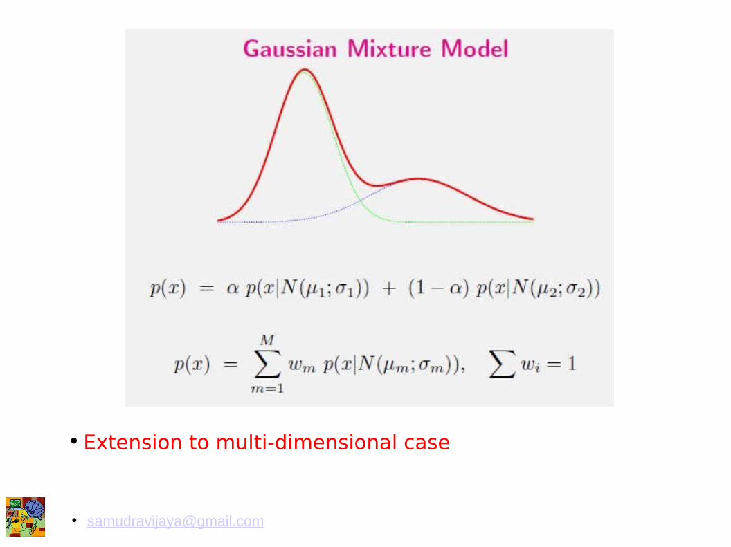
Probability distributions
– Normal (Gaussian) distribution
– Gaussian Mixture Model (GMM)
– Hidden Markov Model (HMM)
● Generation of speech from models
● Overview of HMM based Speech synthesis system (HTS)
● Training of HMMs

Text to Speech Systems
l
l [email protected] Workshop on TTS Synthesis 17-JUN-2014 DAIICT
Waveform concatenation
'Cut-and-paste' approach
Unit selection approach
Speech Model
Articulatory models : Speech production model
Formant : Source-filter model (rules for trajectory)
HTS : Statistical models (machine learning)

Statistical models of speech
[email protected] Workshop on TTS Synthesis 17-JUN-2014 DAIICT
Why statistical models are appropriate (in the context of TTS)?
A lot of variability exists in speech signal due to
Phonetic context
Supra segmental variation: pitch, emphasis, mood.
Models are mathematical expressions of a process / phenomenon in terms of
a small number of parameters.
Statistics provides a succinct method of describing aggregate behaviour of an ensemble.
Statistical models represent an ensemble: a collection of similar entities (ex: phones).
Statistics: Mean, Variance, skewness, kurtosis

•Univariate Gaussian Distribution
• Normal distribution:
• Parameters:– Mean (μ)– Variance (σ2 )
Estimation of parameters

Maximum Likelihood Estimator
Given x[0], x[1], . . . , x[N − 1] and pdf parameterised by θ =
θ1
θ2
.
.
θm−1
We form Likelihood function L(X; θ) =N∏
i=0
p(xi;θ)
θMLE = arg maxθ
L(X; θ)
For height problem:
⇒ can show (θ)MLE = 1N
∑xi
⇒ Estimate of mean of Gaussian = sample mean of measured heights.
WiSSAP 2009: “Tutorial on GMM and HMM”, Samudravijaya K 9 of 88


Multi-modal Distributions
• Distribution of cepstral coefficient of a phone

Training a GMM
• Live demonstration at: http://staff.aist.go.jp/s.akaho/MixtureEM.html
The parameters of a GMM can be trained using
Expectation-Maximization algorithm.
This is an iterative algorithm and consists of 2 steps. It begins with an initial GMM
with (even) random parameters.
In the E-step, an expectation of the log likelihood of the training (adapation) data
given the current GMM is computed.
In the M-step, the parameters of GMM are re-estimated in order to maximise the
expectation of log likelihood.

Generation of speech from statistical models
Consider the vowel ii
Mean StdDevF1 300 100F2 2800 500
Such a normal distribution of formant frequencies of the vowel i can generate a large number of formant values centered around the mean values.
Instead of formants, we can model cepstral coefficients. Then, the corresponding normal distribution can generate any number of MFCCs.
MFCC--> log power spectrum--> speech waveform

l
l [email protected] Workshop on TTS Synthesis 17-JUN-2014 DAIICT

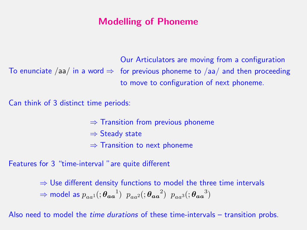
Modelling of Phoneme
To enunciate /aa/ in a word ⇒Our Articulators are moving from a configuration
for previous phoneme to /aa/ and then proceeding
to move to configuration of next phoneme.
Can think of 3 distinct time periods:
⇒ Transition from previous phoneme
⇒ Steady state
⇒ Transition to next phoneme
Features for 3 “time-interval ”are quite different
⇒ Use different density functions to model the three time intervals
⇒ model as paa1(;θaa1) paa2(;θaa
2) paa3(;θaa3)
Also need to model the time durations of these time-intervals – transition probs.
WiSSAP 2009: “Tutorial on GMM and HMM”, Samudravijaya K 36 of 88

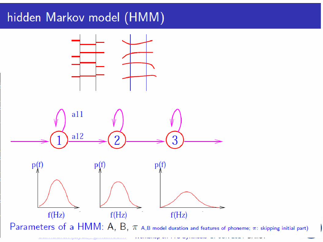
HMM Model of Phoneme
• Use term “State”for each of the three time periods.
• Prob. of ot from jth state, i.e. paaj(ot; θaaj) ⇒ denoted as bj(ot)
1 2 3. . .p(; �1aa) p(; �2aa) p(; �3aa)o10o3o2o1
• Observation, ot, is generated by which state density?
– Only observations are seen, the state-sequence is “hidden”
– Recall: In GMM, the “mixture component is “hidden”
WiSSAP 2009: “Tutorial on GMM and HMM”, Samudravijaya K 38 of 88

What is hidden in hidden Markov model?
Samudravijaya K TIFR, [email protected] Introduction to Automatic Speech Recognition 46/76

HMM Model of Phoneme
• Use term “State”for each of the three time periods.
• Prob. of ot from jth state, i.e. paaj(ot; θaaj) ⇒ denoted as bj(ot)
1 2 3. . .p(; �1aa) p(; �2aa) p(; �3aa)o10o3o2o1
• Observation, ot, is generated by which state density?
– Only observations are seen, the state-sequence is “hidden”
– Recall: In GMM, the “mixture component is “hidden”
WiSSAP 2009: “Tutorial on GMM and HMM”, Samudravijaya K 38 of 88

GMM and HMM
f(Hz)f(Hz)
p(f)
f(Hz)
p(f)
a12
a11
1
p(f)
2 3
Workshop on ASR (Osmania U): “GMM”, [email protected] 48 of 50

How to generate speech from a HMM?
l
l [email protected] Workshop on TTS Synthesis 17-JUN-2014 DAIICT
Input:
– A sentence (sequence of words)
Inventory:
– Pronunciation dictionary
– Trained HMM models for every phone
Output:
Speech waveform
Sentence + pronunciation dictionary
---> sequence of phones
---> sequence of HMM states
---> sequence of feature vectors (source + excitation)
---> speech waveform (using source-filter model)

l Speech Production Model
l
l [email protected] Workshop on TTS Synthesis 17-JUN-2014 DAIICT
Source: Tomoki Toda; WiSSAP 2013

l
l [email protected] Workshop on TTS Synthesis 17-JUN-2014 DAIICT
Source: Tomoki Toda; WiSSAP 2013
These speech parametersshould be modeled
by HMMs

l
l [email protected] Workshop on TTS Synthesis 17-JUN-2014 DAIICT
Source: T.Nagarajan, TTS workshop 2012

l
l [email protected] Workshop on TTS Synthesis 17-JUN-2014 DAIICT
Source: T.Nagarajan, TTS workshop 2012

Speech: A Dynamic Signal
Additional features: Slope and curvature of trajectory: formants/LSPs
Features modeled by HMMs for TTS systems:Cepstral coefficients (MFCC / LPCC)Delta- and delta-delta coefficients
Models for Excitation sourceDurationEmotion

l
l [email protected] Workshop on TTS Synthesis 17-JUN-2014 DAIICT
Source: T.Nagarajan, TTS workshop 2012

System overview of HTS
3 / 15
Training of HMM
Context-DependentHMMs and Duration Models
Label
Mel-cepstral CoefficientsF0
TEXT
Label
SYNTHESIZEDSPEECH
F0
Speech signal
Mel-cepstral Coefficients
Training part
Synthesis part
Parameter Generationfrom HMM
Text Analysis
ExcitationGeneration
MLSAFilter
Mel-cepstralAnalysis
F0Extraction
SPEECHDATABASE

4 / 15
Training part of HTS
PhonemeAlignment
CD-labelsequence
CD-labelsequence
Training data
Context-Dependent HMMs and Duration Models
ContextIndependent
ContextDependent
Initialization and Reestimation
Copy CI-HMMs to CD-HMMs
Embedded Reestimation
Embedded Reestimation
Duration model generation
Tree-based clustering (Spectra)Tree-based clustering (F0)
Tree-based clustering (Duration)
Spectra
F0
Duration

5 / 15
Synthesis part of HTS
State Durations 1 2d d
Mel-cepstrum c c c c cc1 2 3 5 64 cTp p p ppp1 2 3 4 5 6F0 pT
SYNTHESIZEDSPEECH
TEXT
Label
Sentence HMM
State DurationDistributions
Context-Dependent HMMsand Duration Models
Parameter Generation from HMM
d d21
ExcitationGeneration
MLSAFilter
Text analysis

Basic Probability
Joint and Conditional probability (Definitions)
p(A,B) = p(A|B) p(B) = p(B|A) p(A)
Bayes’ rule
p(A|B) =p(B|A) p(A)
p(B)
Workshop on ASR (Osmania U): “GMM”, [email protected] 4 of 50

Basic Probability
Joint and Conditional probability (Definitions)
p(A,B) = p(A|B) p(B) = p(B|A) p(A)
Bayes’ rule
p(A|B) =p(B|A) p(A)
p(B)
If Ais are mutually exclusive events,
p(B)
= p(B|A1)p(A1) + p(B|A2)p(A2) + p(B|A3)p(A3) + ...
=∑
i p(B|Ai) p(Ai)
Workshop on ASR (Osmania U): “GMM”, [email protected] 5 of 50

Basic Probability
Joint and Conditional probability (Definitions)
p(A,B) = p(A|B) p(B) = p(B|A) p(A)
Bayes’ rule
p(A|B) =p(B|A) p(A)
p(B)
If Ais are mutually exclusive events,
p(B)
= p(B|A1)p(A1) + p(B|A2)p(A2) + p(B|A3)p(A3) + ...
=∑
i p(B|Ai) p(Ai)
p(A|B) =p(B|A) p(A)∑i p(B|Ai) p(Ai)
Workshop on ASR (Osmania U): “GMM”, [email protected] 6 of 50

Chain rule
[email protected] Workshop on TTS Synthesis 17-JUN-2014 DAIICT
P( A1, A
2, A
3, ... A
n )
= P( An | A
1, A
2, A
3, ... A
n-1 ) P( A
1, A
2, A
3, ... A
n-1 )
= P( An | A
1, A
2, A
3, ... A
n-1 ) P( A
n-1 | A
1, A
2, A
3, ... A
n-2 )
= P( An | A
1, A
2, A
3, ... A
n-1 ) ... P( A
2 | A
1 ) P(A
1 )

figures/logos/tifrLogo.eps
HMM: definitions
AssumptionsFirst order Markov assumption (finite history):
P(qt = j |qt−1 = i , qt−2 = k, ...) = P(qt = j |qt−1 = i)Stationarity (parameters do not change with time):
P(qt = j |qt−1 = i) = P(qt+l = j |qt+l−1 = i)⇒ exponential duration distribution
Elements of HMMN: number of hidden statesQ: set of states: Q = {q1, q2, q3, ..., qN}B : observation probability distribution: B = {bj} 1 ≤ j ≤ N
A: state transition probability matrix: A = {aij}aij = P(qt+1 = j |qt = i), 1 ≤ i , j ,≤ N
π: initial state distribution:πi = P(q1 = i) 1 ≤ i ≤ N
λ: the entire model: λ = (A,B , π)
Samudravijaya K Workshop on ASR @BAMU; 14-OCT-11 ASR using Hidden Markov Model : A tutorial 10/26

figures/logos/tifrLogo.eps
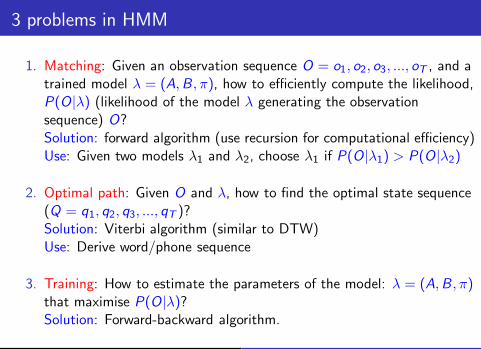
3 problems in HMM
1. Matching: Given an observation sequence O = o1, o2, o3, ..., oT , and atrained model λ = (A,B , π), how to efficiently compute the likelihood,P(O|λ) (likelihood of the model λ generating the observationsequence) O?Solution: forward algorithm (use recursion for computational efficiency)Use: Given two models λ1 and λ2, choose λ1 if P(O|λ1) > P(O|λ2)
Samudravijaya K Workshop on ASR @BAMU; 14-OCT-11 ASR using Hidden Markov Model : A tutorial 11/26

figures/logos/tifrLogo.eps
3 problems in HMM
1. Matching: Given an observation sequence O = o1, o2, o3, ..., oT , and atrained model λ = (A,B , π), how to efficiently compute the likelihood,P(O|λ) (likelihood of the model λ generating the observationsequence) O?Solution: forward algorithm (use recursion for computational efficiency)Use: Given two models λ1 and λ2, choose λ1 if P(O|λ1) > P(O|λ2)
2. Optimal path: Given O and λ, how to find the optimal state sequence(Q = q1, q2, q3, ..., qT )?Solution: Viterbi algorithm (similar to DTW)Use: Derive word/phone sequence
Samudravijaya K Workshop on ASR @BAMU; 14-OCT-11 ASR using Hidden Markov Model : A tutorial 11/26
figures/logos/tifrLogo.eps
3 problems in HMM
1. Matching: Given an observation sequence O = o1, o2, o3, ..., oT , and atrained model λ = (A,B , π), how to efficiently compute the likelihood,P(O|λ) (likelihood of the model λ generating the observationsequence) O?Solution: forward algorithm (use recursion for computational efficiency)Use: Given two models λ1 and λ2, choose λ1 if P(O|λ1) > P(O|λ2)
2. Optimal path: Given O and λ, how to find the optimal state sequence(Q = q1, q2, q3, ..., qT )?Solution: Viterbi algorithm (similar to DTW)Use: Derive word/phone sequence
3. Training: How to estimate the parameters of the model: λ = (A,B , π)that maximise P(O|λ)?Solution: Forward-backward algorithm.
Samudravijaya K Workshop on ASR @BAMU; 14-OCT-11 ASR using Hidden Markov Model : A tutorial 11/26

Training HMMs
[email protected] Workshop on TTS Synthesis 17-JUN-2014 DAIICT
Samudravijaya KTata Institute of Fundamental Research [email protected] [email protected]
Workshop on Text-to-Speech (TTS) Synthesis16-18 June 2014
Dhirubhai Ambani Institute of Information and Communication TechnologyGandhinagar, Gujarat

Training subword HMMs
An iterative algorithm (Baum-Welch, also known asForward-Backward) is used. The Maximum Likelihood approachguarantees increase of the likelihood of the trained model matchingwith training data with each iteration. To begin with, an initialestimation of parameters of HMMs (A,B , π) is required.
Q: How to get an initial estimation of (λ = {A,B , π}?A: We can estimate parameters if we know the boundaries of everysubword HMM in training utterances.
Samudravijaya K TIFR, [email protected] Introduction to Automatic Speech Recognition 58/76

Training subword HMMs
An iterative algorithm (Baum-Welch, also known asForward-Backward) is used. The Maximum Likelihood approachguarantees increase of the likelihood of the trained model matchingwith training data with each iteration. To begin with, an initialestimation of parameters of HMMs (A,B , π) is required.
Q: How to get an initial estimation of (λ = {A,B , π}?A: We can estimate parameters if we know the boundaries of everysubword HMM in training utterances.
Practical solution: Assume that the durations of all units (phones)are equal. If there are N phones in a training utterance, divide thefeature vector sequence into N equal parts. Assign each part, to aphoneme in the phoneme sequence corresponding to thetranscription of the utterance. Repeat for all training utterances.
Samudravijaya K TIFR, [email protected] Introduction to Automatic Speech Recognition 58/76

Basic units of HMM (phone-like units)
a aA i I u U e e� ao aOa A i I u U e E o Ok K g G Rk kh g gh ng C j J � h j jh njV W X Y ZT Th D Dh Nt T d D nt th d dh np P b B mp ph b bh my r l v f q s hy r l w sh S s hSamudravijaya K TIFR, [email protected] Introduction to Automatic Speech Recognition 54/76

Pronunciation dictionary
* Representing a word as a sequence of units of recognition* Pronunciation rules can be used* Manual verification is necessary
kalam vs kamalkarnaa, pahale, Bhaartiyapause
aage aa g e
aaja aa j
aba a b
abbaasa a bb aa s
aatxha aa t’h
Samudravijaya K TIFR, [email protected] Introduction to Automatic Speech Recognition 55/76

Initial estimation of HMM parameters: an illustration
Let the transcription of the 1st wave file be the following sequenceof words: mera bhaarat mahaan
Let the relevant lines in the dictionary be as follows:bhaarata bh aa r a tmahaana m a h aa nmera m e r aa
The phonemeHMM sequence (of length 16) corresponding to thissentence is sil m e r aa bh aa r a t m a h aa n sil
Samudravijaya K TIFR, [email protected] Introduction to Automatic Speech Recognition 59/76

Initial estimation of HMM parameters: an illustration
Let the transcription of the 1st wave file be the following sequenceof words: mera bhaarat mahaan
Let the relevant lines in the dictionary be as follows:bhaarata bh aa r a tmahaana m a h aa nmera m e r aa
The phonemeHMM sequence (of length 16) corresponding to thissentence is sil m e r aa bh aa r a t m a h aa n sil
If the duration of the wavefile is 1.0sec, there will 98 featurevectors (frame shift = 10msec and frame size = 25msec).
Assign the first 6 feature vectors to “sil” HMM; the next 6 (7through 12) to “m”; the next 6 (13 through 18) to “e”; ... ; thelast 8 feature vectors to “sil”. If HMM has 3 states, assign 2feature vector to each state; compute mean,SD.Assume ai ,j=0.5 if j=i or j=i+1; else assign 0.Samudravijaya K TIFR, [email protected] Introduction to Automatic Speech Recognition 59/76

Initial estimation of HMM parameters
[email protected] Workshop on TTS Synthesis 17-JUN-2014 DAIICT
Training data would consist of hundreds of sentences.
For each spoken sentence, repeat the above process: assigning feature vectors to different phonemes of the sentence
Thus, each phone would be assigned several sequences of feature vectors. “m” occurred twice in the previous example; mera bhaarat mahaan
Thus, “m” was allocated 6 feature vectors twice from one speech file

Initial estimation of HMM parameters
[email protected] Workshop on TTS Synthesis 17-JUN-2014 DAIICT
Training data would consist of hundreds of sentences.
For each spoken sentence, repeat the above process: assigning feature vectors to different phonemes of the sentence
Thus, each phone would be assigned several sequences of feature vectors.
“m” occurred twice in the previous example; mera bhaarat mahaan
Thus, “m” was allocated 6 feature vectors twice from one speech file
If a phone is modeled by a 3-state HMM, divide each feature vector sequence into 3 equal
parts. Collect all feature vectors belonging to the first part of the phoneme. Compute mean
and standard deviation: the parameters for the Gaussian distribution N(μ,σ) of the 1st state.
Similarly, estimate the parameters of 2nd and 3rd state of HMM of phoneme “m”
Repeat the above for each phoneme of the language.
We have estimated B = { bj }

Initial estimation of HMM parameters
[email protected] Workshop on TTS Synthesis 17-JUN-2014 DAIICT
We estimated B = { bj } likelihood functions
Let us estimate A = { aij } state transition prob
probabilities
Assign aij
= 0.5 if i=j or j = i+1
0.0 otherwise
Assign = 0.5 for i=1 or 2
Now, we have HMMs for each phoneme: = (A, B, )
by assuming that all phonemes have equal duration !
π
λ π

Better estimation of HMM parameters
[email protected] Workshop on TTS Synthesis 17-JUN-2014 DAIICT
Initial assumption: all phonemes have equal duration
==> boundaries between phonemes are equidistant
100 vectors
16 phones
Adjust the boundaries for better estimation of HMM parameters.
sil m e r aa bh aa r a t m a h aa n sil
sil m e r aa bh aa r a t m a h aa n sil

Re-estimation of HMM parameters
[email protected] Workshop on TTS Synthesis 17-JUN-2014 DAIICT
Adjust the boundaries for better estimation of HMM parameters.
Search for those set of phoneme boundaries such that
the HMM parameters estimated by the revised boundaries
represent the training data better.
Search for the set of phoneme/state boundaries such that the likelihood of
the training data given the current model is the highest.
Then, use this boundary and likelihood information to update the parameters.
sil m e r aa bh aa r a t m a h aa n sil
sil m e r aa bh aa r a t m a h aa n sil

Re-estimation of HMM parameters
[email protected] Workshop on TTS Synthesis 17-JUN-2014 DAIICT
Search for the set of phoneme/state boundaries such that the likelihood of the training data given the revised
parameters is the highest.
We should be able to compute the likelihood of an utterance matching a HMM. In other words,
given an utterance represented by a sequence of observations (O = o1, o
2, o
3, o
4, o
5, o
6, ... o
T)
and a trained HMM = (A, B, ),
we should be able to compute the likelihood P(O | q, )
sil m e r aa bh aa r a t m a h aa n sil
sil m e r aa bh aa r a t m a h aa n sil
λ π
λ

Match a feature vector sequence with a HMM
[email protected] Workshop on TTS Synthesis 17-JUN-2014 DAIICT

[email protected] Workshop on TTS Synthesis 17-JUN-2014 DAIICT
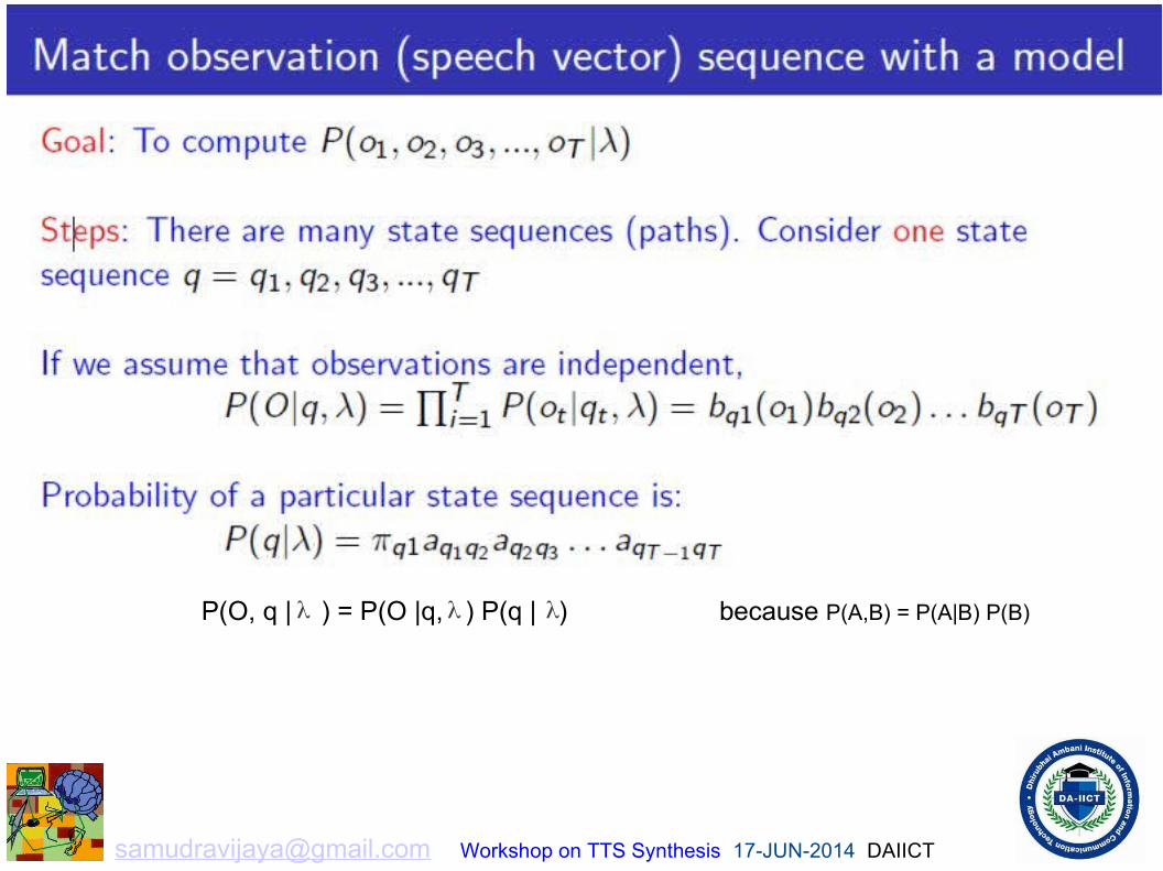
P(O, q | ) = P(O |q, ) P(q | ) because P(A,B) = P(A|B) P(B)λλ λ

figures/logos/tifrLogo.eps
Match observation (speech vector) sequence with a model
Goal: To compute P(o1, o2, o3, ..., oT |λ)
Steps: There are many state sequences (paths). Consider one statesequence q = q1, q2, q3, ..., qT
If we assume that observations are independent,P(O|q, λ) =
∏Ti=1 P(ot |qt , λ) = bq1(o1)bq2(o2) . . . bqT (oT )
Probability of a particular state sequence is:P(q|λ) = πq1aq1q2aq2q3 . . . aqT−1qT
Enumerate paths and sum probabilities:P(O|λ) =
∑qP(O|q, λ)P(q|λ)
⇒ NT state sequences and O(T) calculations⇒ NT O(TNT ) computational complexity: exponential in length!
Samudravijaya K Workshop on ASR @BAMU; 14-OCT-11 ASR using Hidden Markov Model : A tutorial 12/26

figures/logos/tifrLogo.eps
Forward Algorithm: Intution
1
2
3
i
Stat
es
o3 o_t o_t+1 o_T−1 o_T
Observation sequence
i
j
aij
a2j
a_1j
a3j
aNj
N−1
N
o1 o2
Let αt(i) = P(o1, o2, . . . , ot , qt = i |λ). Then
αt+1(j) =∑N
i=1 αt(i)aijbj(ot+1)
Samudravijaya K Workshop on ASR @BAMU; 14-OCT-11 ASR using Hidden Markov Model : A tutorial 13/26

figures/logos/tifrLogo.eps
Forward Algorithm
Define a forward variable αt(i) as:αt(i) = P(o1, o2, . . . , ot , qt = i |λ)
αt(i) is the probability of observing the partial sequence ( o1, o2, . . . , ot)and ot being generated by i th state (i.e., qt = i).
Induction:Initialization:
α1(i) = πibi (o1)Recursion:
αt+1(j) = [∑N
i=1 αt(i)aij ] bj(ot+1)Termination:
P(O|λ) =∑N
i=1 αT (i)
Samudravijaya K Workshop on ASR @BAMU; 14-OCT-11 ASR using Hidden Markov Model : A tutorial 14/26

figures/logos/tifrLogo.eps
Forward Algorithm
Define a forward variable αt(i) as:αt(i) = P(o1, o2, . . . , ot , qt = i |λ)
αt(i) is the probability of observing the partial sequence ( o1, o2, . . . , ot)and ot being generated by i th state (i.e., qt = i).
Induction:Initialization:
α1(i) = πibi (o1)Recursion:
αt+1(j) = [∑N
i=1 αt(i)aij ] bj(ot+1)Termination:
P(O|λ) =∑N
i=1 αT (i)
Computational complexity: O(N2T )
Use: Match a test speech feature vector sequence with all models. Chooseλi if P(O|λi ) > P(O|λj)∀j
Samudravijaya K Workshop on ASR @BAMU; 14-OCT-11 ASR using Hidden Markov Model : A tutorial 14/26

figures/logos/tifrLogo.eps
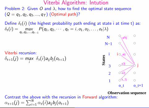
Viterbi Algorithm: IntutionProblem 2: Given O and λ, how to find the optimal state sequence(Q = q1, q2, q3, ..., qT ) (Optimal path)?
Samudravijaya K Workshop on ASR @BAMU; 14-OCT-11 ASR using Hidden Markov Model : A tutorial 15/26

figures/logos/tifrLogo.eps
Viterbi Algorithm: IntutionProblem 2: Given O and λ, how to find the optimal state sequence(Q = q1, q2, q3, ..., qT ) (Optimal path)?
Define δt(i) (the highest probability path ending at state i at time t) as:δt(i) = max
q1,q2,...,qt−1
P(q1, q2, · · · , qt = i , o1, o2, . . . , ot |λ)
1
2
3
i
Stat
es
N−1
N
o_t o_t+1
Observation sequence
i
j
aij
a2j
a_1j
a3j
aNj
Viterbi recursion:δt+1(j) = max
iδt(i)aijbj(ot+1)
Samudravijaya K Workshop on ASR @BAMU; 14-OCT-11 ASR using Hidden Markov Model : A tutorial 15/26
figures/logos/tifrLogo.eps
Viterbi Algorithm: IntutionProblem 2: Given O and λ, how to find the optimal state sequence(Q = q1, q2, q3, ..., qT ) (Optimal path)?
Define δt(i) (the highest probability path ending at state i at time t) as:δt(i) = max
q1,q2,...,qt−1
P(q1, q2, · · · , qt = i , o1, o2, . . . , ot |λ)
1
2
3
i
Stat
es
N−1
N
o_t o_t+1
Observation sequence
i
j
aij
a2j
a_1j
a3j
aNj
Viterbi recursion:δt+1(j) = max
iδt(i)aijbj(ot+1)
Contrast the above with the recursion in Forward algorithm:αt+1(j) =
∑N
i=1 αt(i)aijbj(ot+1)
Samudravijaya K Workshop on ASR @BAMU; 14-OCT-11 ASR using Hidden Markov Model : A tutorial 15/26

figures/logos/tifrLogo.eps
Viterbi AlgorithmInitialization:
δ1(i) = πibi(o1), 1 ≤ i ≤ N
ψ1(i) = 0
Recursion:δt(j) = max
1≤i≤N[δt−1(i)aij ] bj(ot)
ψt(j) = argmax1≤i≤N
[δt−1(i)aij ] 2 ≤ t ≤ T , 1 ≤ j ≤ N
Termination:P∗ = max
1≤i≤N[δT (i)]
q∗T = argmax
1≤i≤N
[δT (i)]
Path (optimal state sequence) backtracking:q∗t = ψt+1(q
∗t+1), t = T − 1,T − 2, · · · , 2, 1.
Samudravijaya K Workshop on ASR @BAMU; 14-OCT-11 ASR using Hidden Markov Model : A tutorial 16/26

figures/logos/tifrLogo.eps
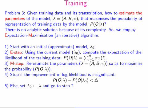
Training
Problem 3: Given training data and its transcription, how to estimate theparameters of the model, λ = (A,B , π), that maximises the probability ofrepresentation of training data by the model, P(O|λ)?There is no analytic solution because of its complexity. So, we employExpectation-Maximisation (an iterative) algorithm.
Samudravijaya K Workshop on ASR @BAMU; 14-OCT-11 ASR using Hidden Markov Model : A tutorial 19/26
figures/logos/tifrLogo.eps
Training
Problem 3: Given training data and its transcription, how to estimate theparameters of the model, λ = (A,B , π), that maximises the probability ofrepresentation of training data by the model, P(O|λ)?There is no analytic solution because of its complexity. So, we employExpectation-Maximisation (an iterative) algorithm.
1) Start with an initial (approximate) model, λ0.2) E-step: Using the current model (λ0), compute the expectation of thelikelihood of the training data: P(O|λ) =
∑Ni=1 αT (i).
3) M-step: Re-estimate the parameters (λ = (A,B , π)) so as to maximisethe probability (P(O|λ)).4) Stop if the improvement in log likelihood is insignificant:
P(O|λ)− P(O|λ0) < ∆5) Else, set λ0 ← λ and go to step 2.
Samudravijaya K Workshop on ASR @BAMU; 14-OCT-11 ASR using Hidden Markov Model : A tutorial 19/26

figures/logos/tifrLogo.eps
Training
Problem 3: Given training data and its transcription, how to estimate theparameters of the model, λ = (A,B , π), that maximises the probability ofrepresentation of training data by the model, P(O|λ)?There is no analytic solution because of its complexity. So, we employExpectation-Maximisation (an iterative) algorithm.
1) Start with an initial (approximate) model, λ0.2) E-step: Using the current model (λ0), compute the expectation of thelikelihood of the training data: P(O|λ) =
∑Ni=1 αT (i).
3) M-step: Re-estimate the parameters (λ = (A,B , π)) so as to maximisethe probability (P(O|λ)).4) Stop if the improvement in log likelihood is insignificant:
P(O|λ)− P(O|λ0) < ∆5) Else, set λ0 ← λ and go to step 2.
The EM algorithm as applied to ASR is known as B-W algorithm; it is alsoknown as Forward-Backward algorithm.
Samudravijaya K Workshop on ASR @BAMU; 14-OCT-11 ASR using Hidden Markov Model : A tutorial 19/26

figures/logos/tifrLogo.eps
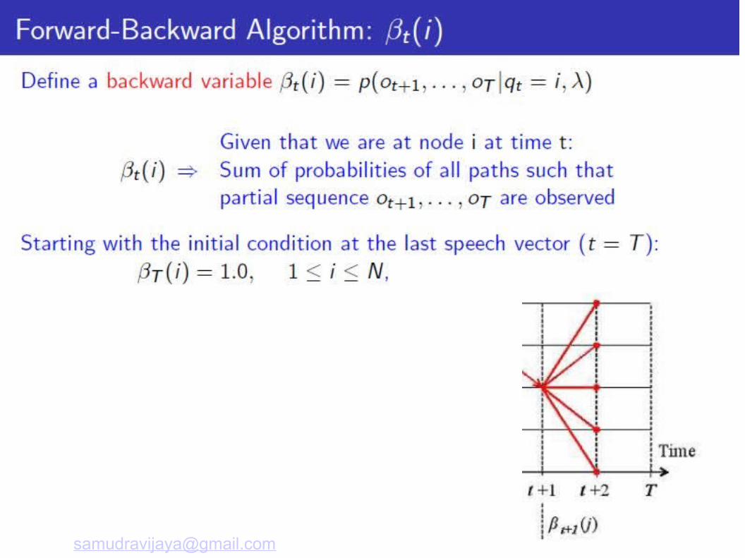
Forward-Backward Algorithm: βt(i)
Define a backward variable βt(i) = p(ot+1, . . . , oT |qt = i , λ)
βt(i)Given that we are at node i at time t:
⇒ Sum of probabilities of all paths such thatpartial sequence ot+1, . . . , oT are observed
Samudravijaya K Workshop on ASR @BAMU; 14-OCT-11 ASR using Hidden Markov Model : A tutorial 20/26

figures/logos/tifrLogo.eps
Forward-Backward Algorithm: βt(i)
Define a backward variable βt(i) = p(ot+1, . . . , oT |qt = i , λ)
βt(i)Given that we are at node i at time t:
⇒ Sum of probabilities of all paths such thatpartial sequence ot+1, . . . , oT are observed
Starting with the initial condition at the last speech vector (t = T ):βT (i) = 1.0, 1 ≤ i ≤ N,
we can recursively compute βt(i) for every state i = 1, 2, . . . ,N backwardsin time (t = T-1, T-2, . . . , 2, 1) as follows:
βt(i) =
N∑
j=1
[aijbj(ot+1)]
︸ ︷︷ ︸Going to each nodefrom i th node
βj(t + 1)︸ ︷︷ ︸
Prob. of observationot+2 . . . oT givennow we are in j th
node at t + 1Samudravijaya K Workshop on ASR @BAMU; 14-OCT-11 ASR using Hidden Markov Model : A tutorial 20/26

figures/logos/tifrLogo.eps
Joint event: state i at time t AND state j at t+1
Define ξt(i , j) as the probability of system being in state i at time t and instate j at time t+1:
ξt(i , j) =αt(i)aijbj (ot+1)βt+1(j)
P(O|λ)
Source: http://www.shokhirev.com/nikolai/abc/alg/hmm/hmm.html
Samudravijaya K Workshop on ASR @BAMU; 14-OCT-11 ASR using Hidden Markov Model : A tutorial 21/26

figures/logos/tifrLogo.eps
Re-estimation Formulae: πi and aij
The revised estimate of initial probability, πi , is the expected frequency instate i at time (t=1):
πnewi =
N∑
j=1
ξ1(i , j)
Samudravijaya K Workshop on ASR @BAMU; 14-OCT-11 ASR using Hidden Markov Model : A tutorial 22/26

Estimating Transition Probability
Trans. Prob. from state i to j = No. of times transition was made from i to jTotal number of times we made transition from i
τt(i, j) ⇒ prob. of being in “state=i at time=t” and “state=j at time=t+1”
If we average τt(i, j) over all time-instants, we get the number of times the system
was in ith state and made a transition to jth state. So, a revised estimation of
transition probability is
anewij =
∑T−1t=1 τt(i, j)
∑Tt=1(
N∑
j=1
τt(i, j)
︸ ︷︷ ︸all transitions out
of i at time=t
)
WiSSAP 2009: “Tutorial on GMM and HMM”, Samudravijaya K 51 of 88

figures/logos/tifrLogo.eps
Re-estimation Formulae: bj(t)
Parameters of State Probability Density FunctionLet us assume that the state output distribution function is Gaussian. Ifthere was just one state j , the maximum likelihood estimation ofparameters would be
µj =1
T
T∑
t=1
ot
Σj =1
T
T∑
t=1
(ot − µj)(ot − µj)′
Samudravijaya K Workshop on ASR @BAMU; 14-OCT-11 ASR using Hidden Markov Model : A tutorial 23/26

figures/logos/tifrLogo.eps
Re-estimation Formulae: bj(t)
Parameters of State Probability Density FunctionLet us assume that the state output distribution function is Gaussian. Ifthere was just one state j , the maximum likelihood estimation ofparameters would be
µj =1
T
T∑
t=1
ot
Σj =1
T
T∑
t=1
(ot − µj)(ot − µj)′
* Difficulty: Speech HMMs have many states.* Speech vector ↔ state mapping is unknown because the state sequenceitself is unknown.* Solution: Assign each speech vector to every state in proportion to thelikelihood of system being in that state when the speech vector wasobserved.
Samudravijaya K Workshop on ASR @BAMU; 14-OCT-11 ASR using Hidden Markov Model : A tutorial 23/26

figures/logos/tifrLogo.eps
Re-estimation Formulae: bj(t)
Let Lj (t) denote the probability of being in state j at time t.
Lj (t) = p(qt = j |O, λ)
=p(qt = j ,O|λ)
p(O|λ)
=αt(i)βt(j)∑
i αT (i)
Samudravijaya K Workshop on ASR @BAMU; 14-OCT-11 ASR using Hidden Markov Model : A tutorial 24/26

figures/logos/tifrLogo.eps
Re-estimation Formulae: bj(t)
Let Lj (t) denote the probability of being in state j at time t.
Lj (t) = p(qt = j |O, λ)
=p(qt = j ,O|λ)
p(O|λ)
=αt(i)βt(j)∑
i αT (i)
Revised estimates of the state pdf parameters are
µj =
∑Tt=1 Lj(t)ot∑Tt=1 Lj(t)
Σj =
∑Tt=1 Lj(t)(ot − µj)(ot − µj)
′
∑Tt=1 Lj(t)
The expected values (estimations) are weighted averages, weights being theprobability of being in state j at time t.
Samudravijaya K Workshop on ASR @BAMU; 14-OCT-11 ASR using Hidden Markov Model : A tutorial 24/26

figures/logos/tifrLogo.eps
Some remarks
Types of HMM* Ergodic Vs left-to-right* Semi-Markov (state duration)* Discriminative models
Implementational Issues* Number of states* Initial parameters* Scaling, addition of logLikelihoods* Multiple observations (tokens/repetitions)* Discrete Vs Continuous probability functions (with GMMs)* Concatenation of smaller HMMs → larger HMM
Samudravijaya K Workshop on ASR @BAMU; 14-OCT-11 ASR using Hidden Markov Model : A tutorial 25/26

figures/logos/tifrLogo.eps
References
◮ Four online tutorials on HMM are listed at< http : //speech.tifr .res.in/tutorials/index .html >
◮ Books: ”Fundamentals of Speech Recognition”, by Lawrence R.Rabiner, B. H. Juang and B.Yegnanarayana, Pearson Education India,2008, Rs. 450; ISBN:9788177585605
◮ Spoken Language Processing : A Guide to Theory, Algorithm andSystem Development, by Xuedong Huang, Alex Acero, Hsiao-WuenHon Year 2001, Prentice Hall PTR; ISBN: 0130226165.
◮ Hidden Markov models for speech recognition; X.D. Huang, Y. Ariki,M.A. Jack. Edinburgh: Edinburgh University Press, c1990.
◮ Statistical methods for speech recognition, F.Jelinek, The MIT Press,Cambridge, MA., 1998.
◮ HMM on MATLAB “HMM toolbox on matlab: Discrete HMMs:training and recognition” by Kevin Murphy, 2005;< http : //www .cs.ubc.ca/ murphyk/Software/HMM/hmm.html >
Samudravijaya K Workshop on ASR @BAMU; 14-OCT-11 ASR using Hidden Markov Model : A tutorial 26/26