higher ocean surface wind speeds during marine cold air

Higher Ocean Surface Wind Speeds During Marine Cold Air Outbreaks

Erik W. Kolstada*

aUni Research Climate, Bjerknes Centre for Climate Research, Bergen, Norway *Correspondence to: Erik W. Kolstad, Uni Research Climate, Allégaten 70, 5007 Bergen, Norway. E-

mail: [email protected] ___________________________________________

Keywords: polar lows; meteorology; cold air outbreaks; mesoscale; air–sea interaction; numerical modelling

Abstract Marine cold air outbreaks (MCAOs) are large-scale phenomena in which cold air masses are advected

over open ocean. It is well-known that these events are linked to the formation of polar lows and other mesoscale phenomena associated with high wind speeds, and that they therefore in some cases represent a hazard to maritime activities. However, it is still unknown whether MCAOs are generally conducive to higher wind speeds than normal. Here this is investigated by comparing the behaviour of ocean surface wind speeds during MCAOs in three atmospheric reanalysis products with different horizontal grid spacings, along with case studies using a convection-permitting numerical weather prediction model. The study regions are the Labrador Sea and the Greenland–Iceland–Norwegian (GIN) Seas, where MCAOs have been shown to be important for air–sea interaction and deep water formation. The main findings are: 1) Wind speeds during the most extreme MCAO events are stronger than normal and higher than wind speeds during less severe events; 2) The peak times of MCAO usually occur when baroclinic waves pass over the regions; and 3) Reanalyses with grid spacings of more than 50 km appear to underestimate winds driven by the large ocean–atmosphere energy fluxes during MCAOs. It is also shown that while the strong wind episodes during MCAOs generally last for just a few days, MCAOs can persist for up to 50 days. These findings demonstrate that it would be worthwhile to forecast MCAOs, and that it might be possible to do this beyond the standard weather forecasting range of up to 10 days.

Preprints (www.preprints.org) | NOT PEER-REVIEWED | Posted: 6 April 2017 doi:10.20944/preprints201704.0035.v1

http://dx.doi.org/10.20944/preprints201704.0035.v1

1. Introduction Events in which cold and dry air masses are transported out from over sea ice or cold land masses over

an area of open ocean are known as marine cold air outbreaks (MCAOs). Such events are important for several reasons. They pose a direct hazard to human activities in that they set up a large energy imbalance which can drive extreme weather. For instance, MCAOs constitute a favourable environment for the formation of polar lows (Kolstad, 2011), intense mesoscale cyclones that form over open ocean at high latitudes (Rasmussen and Turner, 2003). Even when no polar lows form, strong surface wind speeds can occur along Arctic fronts separating cold air masses from warmer air further south (Grønås and Skeie, 1999). The large vertical temperature differences between the ocean surface and the air during MCAOs can give rise to large surface heat fluxes, as measured by numerous in-situ flight campaigns (Grossman and Betts, 1990; Chou and Ferguson, 1991; Brümmer, 1996; Pagowski and Moore, 2001) and with buoys (Harden et al., 2015). One of the mechanisms that arise due to these fluxes are roll clouds or cloud streets, with their large wind speed gradients across small distances (Hartmann et al., 1997; Renfrew and Moore, 1999). In short, MCAOs and associated weather features with high wind speeds are important for air–sea interaction at high latitudes (Våge et al., 2008; Condron and Renfrew, 2013; Isachsen et al., 2013; Papritz and Spengler, 2016).

Figure 1. (a) Advanced Very High Resolution Radar (AVHRR) image taken at 13:44 UTC on 16 January 2005. (b) AVHRR image taken at 21:06 UTC on 25 January 2007. The images are reproduced with the

kind permission of the Dundee Satellite Receiving Station in the UK.

Although MCAOs are linked to known severe weather types, it is still an open question whether MCAOs are generally conducive to high surface wind speeds. If they are, it would mean that MCAOs pose a risk in themselves, even without the presence of polar lows or similar kinds of extreme weather. This question is the main motivation for this study. Using two reanalysis products, the correlations between wind speeds and MCAOs are calculated for two marginal seas in the North Atlantic: the Labrador Sea and the Greenland-



Iceland-Norwegian (GIN) Seas. These regions are known to experience a high frequency of MCAOs during winter (Kolstad et al., 2009; Fletcher et al., 2016). They are also areas in which surface water masses are transformed as a result of interaction with the atmosphere and sea ice (Dickson et al., 1996; Marshall and Schott, 1999).

Figure 1 shows two of the most extreme MCAOs in recent decades in the Labrador Sea and the GIN Seas. In the first of these, roll clouds formed due to advection of cold air masses from the North American continent (Figure 1(a)). The driving force is the low between Greenland and Iceland, and a strong Greenland tip jet event (Doyle and Shapiro, 1999; Moore and Renfrew, 2005) is in progress. In the second case, shown in Figure 1(b), the cold air originates over sea ice and is transported southwards through the Fram Strait between Greenland and Svalbard. The white patches to the south-west of Svalbard is an indication of convection along an elongated high-vorticity shear line which often forms during periods with northerly and north-westerly flow over the Norwegian Sea due to the interaction with the topography and coastline of Spitsbergen (the largest island in the Svalbard archipelago).

There are valid reasons to suppose that wind speeds are higher during MCAOs than in normal conditions. First, the static stability is low during MCAOs, and thus turbulent mixing facilitates downward transmission of wind speed anomalies (Monin and Obukhov, 1954). Second, as the surface heat fluxes during MCAOs can be intense, a strong flow is needed to prevent the cold air masses from being heated so much from below that the MCAO expires (Papritz and Pfahl, 2015). The third reason has already been mentioned: multiple small-scale features, such as the ones observed in the satellite images in Figure 1, commonly occur in MCAO conditions.

There is also cause to believe that the strong winds during MCAOs are not always captured by reanalyses. For instance, it has been demonstrated that ERA-Interim does not fully reproduce polar lows (Zappa et al., 2014; Pezza et al., 2016). The reason is that the spatial scale of several phenomena is too small for reanalyses to be even theoretically able to reproduce them. At least four, and sometimes up to ten, grid points are required to resolve wave-like mesoscale features (Walters, 2000). The grid spacing (Δ ) of ERA-Interim (Dee et al., 2011) is 80 km, which means that it cannot features on scales of less than 300 km. One example of a small-scale feature pertinent for this study is the shear line south of Svalbard, of which an example was shown in Figure 1(b). A case study by Sergeev et al. (2016) indicated that the maximum horizontal wind speed gradient across one such shear line was 25 m s–1 over just 50 km, less than theΔ of ERA-Interim and identical to theΔ of the second version of the Modern Era Retrospective analysis for Research and Applications (MERRA) reanalysis (Rienecker et al., 2011). A related phenomenon is the topography-induced Greenland tip jet that forms near Cape Farewell. A model-based case study showed that decreases of Δ from 100, 50, and 25 km to 10 km led to stepwise improvements in the representation of tip jets (DuVivier and Cassano, 2013). As for polar lows, decreasing Δ from 12 to 4 km ‘significantly improved’ the simulation of two cases over the Norwegian Sea (McInnes et al., 2011).

A consequence of the coarse resolution of the reanalyses is that reanalysis-based correlations between MCAOs and wind speed may misrepresent the actual relationship between the variables. The evidence of underestimation of wind speeds during MCAOs in reanalysis products abounds. Substantial improvements in the representation wind speeds have been shown for the Arctic System Reanalysis (ASR; Bromwich et al., 2016) for several small-scale features, including southeast Greenland barrier winds and katabatic flows (Moore et al., 2015), and topographically forced winds near Greenland (Moore et al., 2016), tip jets included. The grid spacing of the ASR is 30 km. To illustrate how small-scale wind features not resolved by reanalyses can arise during MCAOs, case studies of some of the most extreme MCAOs during the reanalysis period are performed with a convection-permitting numerical simulation (Δ = 4 km).

This study is structured around the search for answers to three broad questions designed to shed light on the role of MCAOs in driving surface wind speeds over the ocean, with implications for maritime activities and air–sea interaction. The first question is: What is the relationship between the severity of MCAOs and associated wind speeds? To investigate this, MCAO events are detected using time series of an established MCAO index. The events are then ranked by severity, and the wind speeds during the events are studied.



The second question is: How do MCAOs and associated wind speeds evolve? By studying the 100 most intense events in each region, composite averages of wind speed, surface pressure and the MCAO index are calculated and studied. The third question addresses the known fact that MCAOs form a favourable environment for mesoscale features not necessarily resolved by reanalysis products, and is formulated as follows: Do reanalyses with a grid spacing of 50 km or more underestimate the actual relationship between MCAOs and wind speeds? This is explored by performing case studies of two extreme MCAOs, where wind speeds simulated using a convection-permitting model are compared with wind speeds from the reanalyses.

2. Data and Methods Here I follow Papritz et al. (2015) and use an MCAO index defined as = − , where is

the potential temperature at 850 hPa, and is the ‘potential skin temperature’, calculated as =, where is the skin temperature, is the surface pressure, and is 1000 hPa. November

to March (NDJFM) data from ERA-Interim and MERRA-2 are used for the period 1980–2016, as this period was available for both data sets when the analysis was performed. The ASR, which only covers the period 2000–2012, is used for comparison with the other reanalyses.

Figure 2. Monthly mean skin temperature (filled contours) and the approximate sea ice edge (white contours) in MERRA-2 for January 2016. The two study regions are shown as black polygons: the GIN

Seas (20°W–17°E and 66.5°N–76.5°N) and the Labrador Sea (65°W–43°W and 52°N–60°N).

The MCAO index is computed for each grid point and then area-averaged for two regions: the GIN Seas and the Labrador Sea. These regions are drawn as boxes in Figure 2, where the monthly mean MERRA-2 skin temperature and the approximate sea ice edge (contoured sea ice fraction for the value 0.55) are also shown. Land grid cells and cells for which the skin temperature is lower than 271.5 K is not included when area-averaging. Ten-meter wind speed and the meridional wind component are also area-averaged for the



same grid cells. Anomalies are calculated with respect to the overall mean values for each month, day and time.

For each region, time series of 12-hourly values of the MCAO index M are used to identify events. A new event is started when > 0 K and ended if < 0 K for two successive time steps. This is done to merge two neighbouring events when they are separated by only one time step with < 0 K. After an event is terminated, the last time that > 0 K is set as the last time of the event. Events are only recorded if they attain an M value of at least 3 K and last at least 48 hours. The peak of each event is required to occur in NDJFM, but the events are allowed to start in October or end in April. Using this algorithm, each event is separated from its neighbouring events by at least 48 hours.

Different values for M have been used in other studies. Fletcher et al. (2016) used 3 K as a lower threshold for moderate MCAO events, using air temperatures at the 800 hPa level. Papritz et al. (2015) applied five thresholds ranging from 0 K to 8 K, yielding different intensity categories. Here a single threshold of 3 K is used, but for one part of the analysis the MCAO events are ranked according to their highest M value. The results do not change appreciably when other nearby thresholds are used instead.

Two case studies, one for each region, are performed to compare winds speeds from convection-permitting simulations with winds speeds from the reanalysis products during extreme MCAOs. Version 3.7.1 of the Weather and Research Forecasting (WRF) model is used, with three-hourly ERA-Interim data as boundary and initial forcing. The simulations are initiated 48 hours prior to the peaks of the MCAO index. Inner domains with Δ = 4 km are nested inside outer domains with Δ = 12km. Except for the slightly larger Δ , the WRF configuration used follows one that was found to successfully represent the main features of a hurricane-like polar low in the Barents Sea (Kolstad and Bracegirdle, 2016). Cumulus parameterisation is switched off. Note also that spectral nudging (von Storch et al., 2000) of winds and temperature above 700 hPa is applied in the outer domain, with a nudging wavelength of 1100 km. Sea surface temperatures and the sea ice fraction are kept fixed throughout the simulations. QuikSCAT satellite-derived wind speeds (Hoffman and Leidner, 2005) are used for validation.

3. Results 3.1. MCAO events ranked by intensity

The first question posed in the introduction relates to the relationship between the severity of MCAOs and their associated wind speeds. For the two study regions, about 300 events were identified using the algorithm described in the previous section. Events occur more frequently in the Labrador Sea than in the GIN Seas. The dots in Figure 3 show the wind speed anomalies during the peak of each event (i.e., the time of the highest M value). The x-axes show the rank of each event (the first event is the one with the highest overall M value). The black dots show wind speed anomalies during events for which the area-averaged meridional wind during the M peak was negative (northerly flow), and grey dots indicate southerly flow. About 70% of the Labrador Sea events and practically all the events in the GIN Seas occurred in northerly flow. The lines show the best linear fit to the wind speed anomalies, calculated using least squares. To assess the statistical significance of the linear fits, the Spearman’s rank correlations (Spearman, 1904), also known as Spearman’s , between the x values and the rank of each y value in each graph were calculated. These are listed above each panel. Each value is statistically significant at the 10–5 level. The differences between the highest and lowest points along the linear fits shown in Figure 3(a) are 3.7 m s–1 in ERA-Interim and 4.6 m s–1 in MERRA-2 (Figure 3(b)). In the GIN Seas region, the differences are 1.8 and 1.9 m s–1, respectively, as shown in Figure 3(c) and (d). This analysis was also performed for the ASR, where 113 events were identified in the Labrador Sea and 98 in the GIN Seas. The negative values are significant at the 5% level in both regions, despite the smaller number of events due to the shorter period. The differences between the most and least intense events according to the linear fits are 2.5 m s–1 in the Labrador Sea (less than what was found for the other reanalyses) and 2.0 m s–1 in the GIN Seas (slightly higher than for the other reanalyses).



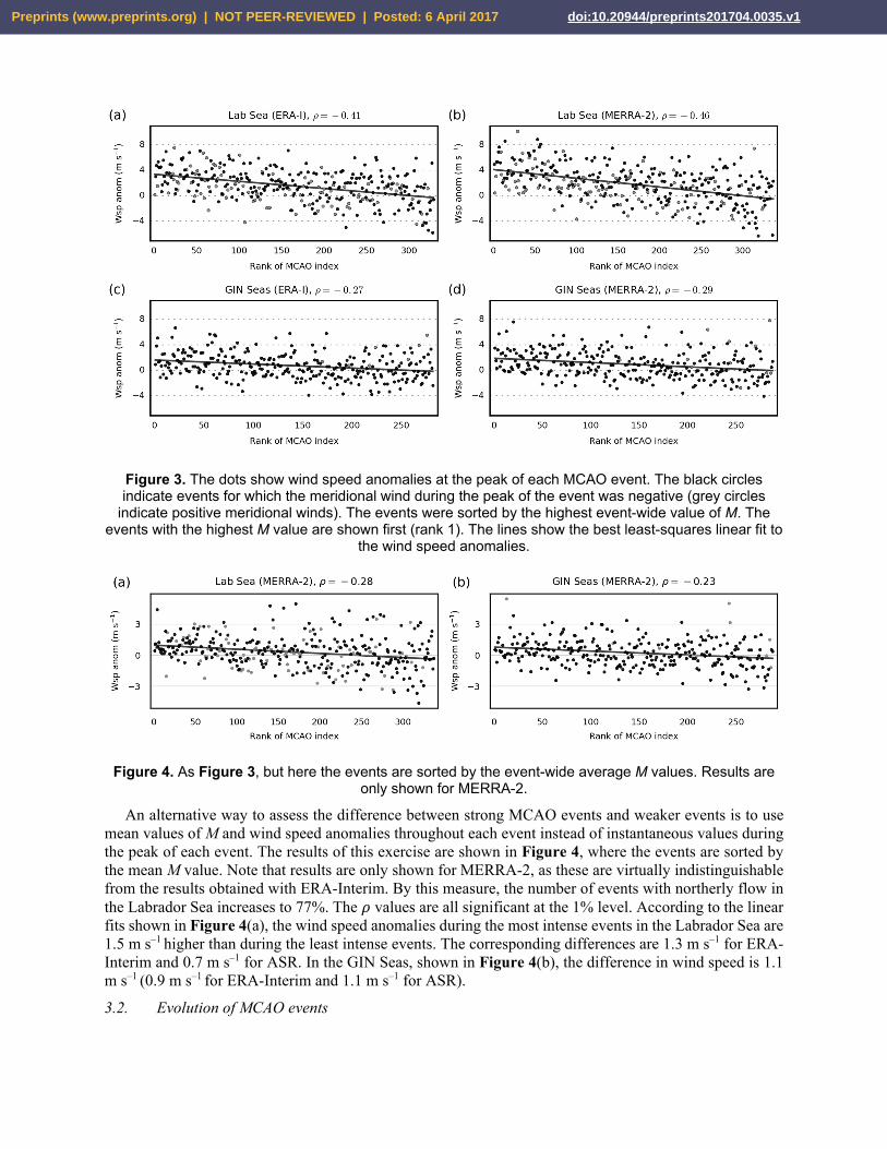
Figure 3. The dots show wind speed anomalies at the peak of each MCAO event. The black circles indicate events for which the meridional wind during the peak of the event was negative (grey circles

indicate positive meridional winds). The events were sorted by the highest event-wide value of M. The events with the highest M value are shown first (rank 1). The lines show the best least-squares linear fit to

the wind speed anomalies.

Figure 4. As Figure 3, but here the events are sorted by the event-wide average M values. Results are only shown for MERRA-2.

An alternative way to assess the difference between strong MCAO events and weaker events is to use mean values of M and wind speed anomalies throughout each event instead of instantaneous values during the peak of each event. The results of this exercise are shown in Figure 4, where the events are sorted by the mean M value. Note that results are only shown for MERRA-2, as these are virtually indistinguishable from the results obtained with ERA-Interim. By this measure, the number of events with northerly flow in the Labrador Sea increases to 77%. The values are all significant at the 1% level. According to the linear fits shown in Figure 4(a), the wind speed anomalies during the most intense events in the Labrador Sea are 1.5 m s–1 higher than during the least intense events. The corresponding differences are 1.3 m s–1 for ERA-Interim and 0.7 m s–1 for ASR. In the GIN Seas, shown in Figure 4(b), the difference in wind speed is 1.1 m s–1 (0.9 m s–1 for ERA-Interim and 1.1 m s–1 for ASR).

3.2. Evolution of MCAO events



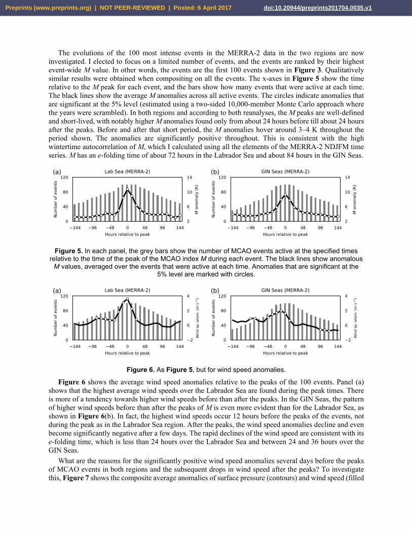
The evolutions of the 100 most intense events in the MERRA-2 data in the two regions are now investigated. I elected to focus on a limited number of events, and the events are ranked by their highest event-wide M value. In other words, the events are the first 100 events shown in Figure 3. Qualitatively similar results were obtained when compositing on all the events. The x-axes in Figure 5 show the time relative to the M peak for each event, and the bars show how many events that were active at each time. The black lines show the average M anomalies across all active events. The circles indicate anomalies that are significant at the 5% level (estimated using a two-sided 10,000-member Monte Carlo approach where the years were scrambled). In both regions and according to both reanalyses, the M peaks are well-defined and short-lived, with notably higher M anomalies found only from about 24 hours before till about 24 hours after the peaks. Before and after that short period, the M anomalies hover around 3–4 K throughout the period shown. The anomalies are significantly positive throughout. This is consistent with the high wintertime autocorrelation of M, which I calculated using all the elements of the MERRA-2 NDJFM time series. M has an e-folding time of about 72 hours in the Labrador Sea and about 84 hours in the GIN Seas.

Figure 5. In each panel, the grey bars show the number of MCAO events active at the specified times relative to the time of the peak of the MCAO index M during each event. The black lines show anomalous

M values, averaged over the events that were active at each time. Anomalies that are significant at the 5% level are marked with circles.

Figure 6. As Figure 5, but for wind speed anomalies.

Figure 6 shows the average wind speed anomalies relative to the peaks of the 100 events. Panel (a) shows that the highest average wind speeds over the Labrador Sea are found during the peak times. There is more of a tendency towards higher wind speeds before than after the peaks. In the GIN Seas, the pattern of higher wind speeds before than after the peaks of M is even more evident than for the Labrador Sea, as shown in Figure 6(b). In fact, the highest wind speeds occur 12 hours before the peaks of the events, not during the peak as in the Labrador Sea region. After the peaks, the wind speed anomalies decline and even become significantly negative after a few days. The rapid declines of the wind speed are consistent with its e-folding time, which is less than 24 hours over the Labrador Sea and between 24 and 36 hours over the GIN Seas.

What are the reasons for the significantly positive wind speed anomalies several days before the peaks of MCAO events in both regions and the subsequent drops in wind speed after the peaks? To investigate this, Figure 7 shows the composite average anomalies of surface pressure (contours) and wind speed (filled



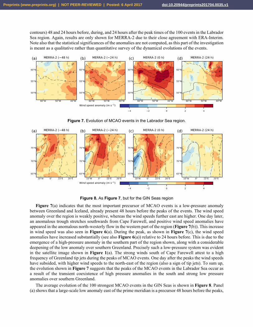
contours) 48 and 24 hours before, during, and 24 hours after the peak times of the 100 events in the Labrador Sea region. Again, results are only shown for MERRA-2 due to their close agreement with ERA-Interim. Note also that the statistical significances of the anomalies are not computed, as this part of the investigation is meant as a qualitative rather than quantitative survey of the dynamical evolutions of the events.

Figure 7. Evolution of MCAO events in the Labrador Sea region.

Figure 8. As Figure 7, but for the GIN Seas region

Figure 7(a) indicates that the most important precursor of MCAO events is a low-pressure anomaly between Greenland and Iceland, already present 48 hours before the peaks of the events. The wind speed anomaly over the region is weakly positive, whereas the wind speeds further east are higher. One day later, an anomalous trough stretches southwards from Cape Farewell, and positive wind speed anomalies have appeared in the anomalous north-westerly flow in the western part of the region (Figure 7(b)). This increase in wind speed was also seen in Figure 6(a). During the peak, as shown in Figure 7(c), the wind speed anomalies have increased substantially (see also Figure 6(a)) relative to 24 hours before. This is due to the emergence of a high-pressure anomaly in the southern part of the region shown, along with a considerable deepening of the low anomaly over southern Greenland. Precisely such a low-pressure system was evident in the satellite image shown in Figure 1(a). The strong winds south of Cape Farewell attest to a high frequency of Greenland tip jets during the peaks of MCAO events. One day after the peaks the wind speeds have subsided, with higher wind speeds to the north-east of the region (also a sign of tip jets). To sum up, the evolution shown in Figure 7 suggests that the peaks of the MCAO events in the Labrador Sea occur as a result of the transient coexistence of high pressure anomalies in the south and strong low pressure anomalies over southern Greenland.

The average evolution of the 100 strongest MCAO events in the GIN Seas is shown in Figure 8. Panel (a) shows that a large-scale low anomaly east of the prime meridian is a precursor 48 hours before the peaks,



along with a less pronounced high anomaly along the east coast of Greenland. Together these pressure anomalies yield anomalous northerly flow into the region. The average wind speed anomaly is already positive, especially in the northern part of the region. The above-average wind speeds agree with Figure 6(b). One day before the peaks, the wind speeds have increased additionally, as shown in Figure 8(b). The chief cause appears to be enhanced pressure gradients, mainly due to a further development of the ridge east of Greenland. Another likely cause is the twin influences of the sea ice edge and the topography of Spitsbergen (see Figure 1(b)). During the peaks of the MCAO events, the wind speed over the region is still high, as shown in Figure 8(c). Recall that the peak in wind speed occurs 12 hours before the peaks (Figure 6(b)). The primary change from 24 hours before is a rapid strengthening of the ridge east of Greenland. Figure 8(d) shows that the pressure gradients are weak one day after the peaks. The average wind speed anomalies are also weak at this point, as already indicated by the rapid decline in wind speed shown in Figure 6(b).

3.3. Case studies of two MCAO events

Figure 9. Wind speeds at 09:00 UTC on 16 January 2005, according to ERA-Interim (a), MERRA-2 (b), the ASR (c), the WRF simulation (d), and QuikSCAT (e). The latter map is combined from several

QuikSCAT retrievals. White contours are drawn along the 25 m s–1 isoline, and the black contours show the approximate ice edge. The white patches in (e) appear because QuikSCAT data are not available

near land or the sea ice edge.

To illustrate the impact of model grid spacing on the representation of small-scale winds during MCAOs, one event in each region is investigated in detail. For the Labrador Sea, the event with the highest peak M value during 2000–2009 is studied. This period was chosen because there is data available for four datasets: ERA-Interim, MERRA-2, ASR, and QuikSCAT. A WRF simulation with Δ = 4 km was performed, starting at 12:00 UTC on 14 January 2005. The satellite image in Figure 1(a) was taken at 13:33 UTC on



16 January. Figure 9(a–d) shows the 10-metre wind speed at 09:00 UTC on the same day for the reanalyses and the WRF simulation. The black contours indicate the approximate sea ice edge. The QuikSCAT data shown in Panel (e) was retrieved between 08:05 and 10:06 on the same day. The white areas reflect missing QuikSCAT data over and near sea ice and land. The white contours in all the panels show the 25 m s–1

isoline.

The QuikSCAT image reveals a strong tip jet event. This is also reproduced by all the models, although the magnitudes of the wind speeds vary. WRF produces more small-scale detail than the other models, and this matches the roll cloud structures seen in Figure 1(a). The wind speed associated with the tip jet for both WRF and the ASR, and to some extent MERRA-2, agree quite well with QuikSCAT. There is also a region with high wind speeds near 50°W and 55°N which is captured only by WRF and the ASR. The ASR shows a wake region near Cape Farewell which does not appear to be correct (judging from the QuikSCAT imagery), but that could be related to an error in the timing of the low to the west of Iceland rather than grid spacing. The tip jet wind speed in ERA-Interim is too low.

Figure 10. As Figure 9, but for the GIN Seas region at 21:00 UTC on 25 January 2007, and with white contours showing the 20 m s–1 isoline.

The highest MCAO index value in the GIN Seas region in the period 2000–2009 occurred on 26 January 2007. The satellite image in Figure 1(b) was taken at 21:06 UTC on 25 January. Figure 10 shows simulated wind speeds at 21:00 UTC on that day, along with QuikSCAT data retrieved between 19:12 and 23:14 UTC. In these maps the white contours are drawn at 20 m s–1. The wake downstream of Spitsbergen is best reproduced by the ASR and WRF. Of these WRF is the only model that gives wind speeds comparable with



QuikSCAT in the area to the west of Spitsbergen. The small-scale structures associated with the roll clouds are only reproduced by WRF. Both ERA-Interim and MERRA-2, and to some degree the ASR, give too low wind speeds over much of the GIN Seas. In particular, the strong winds along the shear zone south of Spitsbergen, which is also evident in the satellite image in Figure 1(b), is adequately resolved only by WRF. This is therefore another example of underestimation of the true wind speeds during a strong MCAO in the coarser-resolution reanalyses.

4. Summary and discussion The first question in the Introduction was: What is the relationship between the severity of MCAOs and

associated wind speeds? The results presented here clearly show that the most severe MCAO events coincide with stronger wind speeds than weaker events. Although not discussed earlier, the overall (i.e., using all times, not just during MCAO events) correlations between anomalies of the MCAO index M and wind speed are statistically significant at the 10–10 level in both regions, both at lag-0 and when the wind speeds lead M by up to several days. This demonstrates that MCAOs are associated with above-average wind speeds.

The second question was: How do MCAOs and associated wind speeds evolve? The long e-folding time of the MCAO index and the composite analysis of MCAO events indicate that strong MCAOs commence when the MCAO index is already high. In the Labrador Sea region, the existence of a low-pressure anomaly between Iceland and Greenland is a precursor 48 hours before the peaks of strong MCAO events. In the GIN Seas, northerly winds over the region are a precursor 48 hours before the peaks. The peaks in both regions occur when ridges and troughs rapidly develop to create a flow that is optimal for transporting cold air masses over the region. The rapid build-up and the overall transient nature of the peaks of the events indicate that they are associated with passages of baroclinic waves. This result is consistent with the findings of Fletcher et al. (2016), who concluded that strong MCAOs occur in the cold air sector of mid-latitude cyclones. It is also interesting to note that MCAOs are essentially self-destructive. The vigorous transfer of energy from the ocean to the atmosphere becomes more effective when the wind speed is high, which it is during the peaks of the events. This energy transfer leads to a cooling of the sea surface and a warming of the lower atmosphere through sensible heat fluxes and latent heating (Papritz and Pfahl, 2015), and thereby forces a decrease in the MCAO index. The MCAO will therefore extinguish itself unless it is reinforced by fresh, incoming cold air masses due to some external factor.

The third and final question was: Do reanalyses with a grid spacing of 50 km or more underestimate the actual relationship between MCAOs and wind speeds? As only two case studies were investigated, a complete answer is elusive. Perhaps the upcoming 10 km version of the ASR, or similar products, can help answer this question more conclusively. The case studies performed here, in which the 30 km version of the ASR was used, indicate that a dense grid spacing (less than 30 km) is required to obtain an accurate reproduction of the actual small-scale ocean surface wind speeds during strong MCAOs. As mentioned, previous studies have also shown that reanalyses do not fully resolve some severe weather features associated with MCAOs, such as polar lows. Thus, the answer to the third question is a qualified ‘Yes’.

One key finding is that MCAOs are large-scale phenomena that can last for days and even weeks. The longest events in both regions lasted for over 50 days. As mentioned, the e-folding time of the MCAO index is about 72 hours in the Labrador Sea and about 84 hours in the GIN Seas. It is therefore possible that MCAOs can be forecast on the sub-seasonal time scale, i.e. beyond 5–10 days, which is the typical range of numerical weather prediction. Cai et al. (2015) claimed that continental-scale cold air outbreaks can be forecast up to one month ahead by means of a hybrid statistical/dynamical model system, using key indices for stratospheric circulation as predictors. The lagged association between stratospheric polar vortex anomalies and subsequent cold air outbreaks in winter has been the topic of many studies (e.g. Thompson et al., 2002; Kolstad et al., 2010). It is also possible that empirical indices based on SST anomalies and sea ice can be used for forecasting purposes. If MCAOs can be forecast on the sub-seasonal time scale, there might be a potential for developing early warning systems for severe weather in marine environments. This



is proposed as important future work with potentially high relevance for stakeholders in coastal, Arctic regions.

The relationship between MCAOs and wind speeds also has implications for air–sea interaction and thereby possibly also for convection in the ocean. It has for instance been shown that Greenland tip jet events have an impact on deep convection in the Irminger Sea south of Iceland (Våge et al., 2008). The comparisons between the reanalysis products and the high-resolution ASR and WRF simulations also suggested that wind speeds are underestimated in coarse-resulution reanalyses. In a series of papers, Alan Condron and his colleagues first showed that polar mesocyclones (including polar lows) were not adequately represented by the ERA-40 reanalysis (Condron et al., 2006), and then used a ‘bogusing’ approach to parameterise these cyclones in ocean model experiments (Condron et al., 2008). Compared with model runs with no parameterisation, they found ‘increases in the simulated depth, frequency and area of deep convection in the Nordic seas, which in turn leads to a larger northward transport of heat into the region, and southward transport of deep water through Denmark Strait’ (Condron and Renfrew, 2013). Similar results were obtained by Jung et al. (2014), who compared ocean model simulations forced with high- and low-resolution atmospheric data. In a related study by Holdsworth and Myers (2015), coupled ocean–ice model simulations forced with hourly atmospheric data were compared with simulations where the high-frequency atmospheric forcing was filtered out. In the Labrador Sea, these differences yielded large changes in the oceanic mixed layer depth. These studies imply that there is a great potential for parameterising MCAOs in ocean models, perhaps in ways that can make use of the results presented here.

5. Conclusions Severe MCAO events tend to arise when the background flow is favourable, meaning that the wind

direction is such that cold air is already being advected over the ocean. The peaks of the events coincide with the passages of rapidly moving baroclinic waves. A key factor is ridging, which contributes to enhanced pressure gradients and a stronger flow of cold air. High wind speed anomalies occur a few days before and during the peaks of the events. After the peaks, however, the wind speeds subside rapidly. But although the strong wind episodes are transient, MCAOs can be sustained for up to 50 days. High-resolution model experiments indicate that the actual correlation between wind speed and severe MCAOs could be higher than what is indicated by reanalysis products with a grid spacing of 50 km or more.

Acknowledgments The author thanks Lukas Papritz, Tom Bracegirdle and Kjetil Våge for constructive discussions during

the writing process. He also thanks the ECMWF for providing the ERA-Interim reanalysis data, the Global Modeling and Assimilation Office (GMAO) at NASA Goddard Space Flight Center, who provided the MERRA-2 data, the Byrd Polar Research Center at the University of Ohio and NCAR (thanks to Chi-Fan Shih) for producing and providing the ASR data, and the vast community that has developed and continues to maintain the WRF model. The satellite images are reproduced with the kind permission of the Dundee Satellite Receiving Station in the UK (thanks to Neil Lonie). The author’s work was funded by the European Commission through the Blue Action project (grant 727852).

References Bromwich DH, Wilson AB, Bai L-S, Moore GW, Bauer P. 2016. A comparison of the regional Arctic

System Reanalysis and the global ERA-Interim Reanalysis for the Arctic. Q. J. R. Meteorol. Soc. 142: 644–658.

Brümmer B. 1996. Boundary-layer modification in wintertime cold-air outbreaks from the Arctic sea ice. Boundary Layer Meteorol. 80: 109-125.



Cai M, Yu Y, Deng Y, van den Dool HM, Ren R, Saha S, Wu X, Huang J. 2015. Feeling the Pulse of the Stratosphere: An Emerging Opportunity for Predicting Continental-Scale Cold-Air Outbreaks 1 Month in Advance. Bull. Am. Meteorol. Soc. 97: 1475-1489.

Chou SH, Ferguson MP. 1991. Heat fluxes and roll circulations over the western Gulf Stream during an intense cold-air outbreak. Boundary Layer Meteorol. 55: 255-281.

Condron A, Bigg GR, Renfrew IA. 2006. Polar Mesoscale Cyclones in the Northeast Atlantic: Comparing Climatologies from ERA-40 and Satellite Imagery. Mon. Weather Rev. 134: 1518-1533.

Condron A, Bigg GR, Renfrew IA. 2008. Modeling the impact of polar mesocyclones on ocean circulation. J. Geophys. Res. 113: C10005.

Condron A, Renfrew IA. 2013. The impact of polar mesoscale storms on northeast Atlantic Ocean circulation. Nat. Geosci.

Dee DP, Uppala SM, Simmons AJ, Berrisford P, Poli P, Kobayashi S, Andrae U, Balmaseda MA, Balsamo G, Bauer P, Bechtold P, Beljaars ACM, van de Berg L, Bidlot J, Bormann N, Delsol C, Dragani R, Fuentes M, Geer AJ, Haimberger L, Healy SB, Hersbach H, Hólm EV, Isaksen L, Kållberg P, Köhler M, Matricardi M, McNally AP, Monge-Sanz BM, Morcrette JJ, Park BK, Peubey C, de Rosnay P, Tavolato C, Thépaut JN, Vitart F. 2011. The ERA-Interim reanalysis: Configuration and performance of the data assimilation system. Q. J. R. Meteorol. Soc. 137: 553-597.

Dickson R, Lazier J, Meincke J, Rhines P, Swift J. 1996. Long-term coordinated changes in the convective activity of the North Atlantic. Progress in Oceanography. 38: 241-295.

Doyle JD, Shapiro MA. 1999. Flow response to large‐scale topography: The Greenland tip jet. Tellus. 51A: 728–748.

DuVivier AK, Cassano JJ. 2013. Evaluation of WRF Model Resolution on Simulated Mesoscale Winds and Surface Fluxes near Greenland. Mon. Weather Rev. 141: 941–963.

Fletcher J, Mason S, Jakob C. 2016. The Climatology, Meteorology, and Boundary Layer Structure of Marine Cold Air Outbreaks in Both Hemispheres. J. Clim. 29: 1999–2014.

Grossman RL, Betts AK. 1990. Air–Sea Interaction during an Extreme Cold Air Outbreak from the Eastern Coast of the United States. Mon. Weather Rev. 118: 324–342.

Grønås S, Skeie P. 1999. A case study of strong winds at an Arctic front. Tellus. 51A: 865–879. Harden BE, Renfrew IA, Petersen GN. 2015. Meteorological buoy observations from the central Iceland

Sea. J. Geophys. Res. Atmos. 120: 3199-3208. Hartmann J, Kottmeier C, Raasch S. 1997. Roll Vortices and Boundary-Layer Development during a Cold

Air Outbreak. Boundary Layer Meteorol. 84: 45–65. Hoffman RN, Leidner SM. 2005. An Introduction to the Near-Real-Time QuikSCAT Data. Weather

Forecast. 20: 476–493. Holdsworth AM, Myers PG. 2015. The Influence of High-Frequency Atmospheric Forcing on the

Circulation and Deep Convection of the Labrador Sea. J. Clim. 28: 4980–4996. Isachsen PE, Drivdal M, Eastwood S, Gusdal Y, Noer G, Saetra Ø. 2013. Observations of the ocean

response to cold air outbreaks and polar lows over the Nordic Seas. Geophys. Res. Lett. 40: 3667-3671.

Jung T, Serrar S, Wang Q. 2014. The oceanic response to mesoscale atmospheric forcing. Geophys. Res. Lett. 41: 1255-1260.

Kolstad EW, Bracegirdle TJ, Seierstad IA. 2009. Marine cold-air outbreaks in the North Atlantic: temporal distribution and associations with large-scale atmospheric circulation. Clim. Dyn. 33: 187–197.

Kolstad EW, Breiteig T, Scaife AA. 2010. The association between stratospheric weak polar vortex events and cold air outbreaks in the Northern Hemisphere. Q. J. R. Meteorol. Soc. 136: 886–893.

Kolstad EW. 2011. A global climatology of favourable conditions for polar lows. Q. J. R. Meteorol. Soc. 137: 1749–1761.

Kolstad EW, Bracegirdle TJ. 2016. Sensitivity of an Apparently Hurricane-like Polar Low to Sea Surface Temperature. Q. J. R. Meteorol. Soc.: in press.

Marshall J, Schott F. 1999. Open-ocean convection: Observations, theory, and models. Rev. Geophys. 37: 1-64.



McInnes H, Kristiansen J, Kristjánsson JE, Schyberg H. 2011. The role of horizontal resolution for polar low simulations. Q. J. R. Meteorol. Soc. 137: 1674–1687.

Monin A, Obukhov A. 1954. Basic laws of turbulent mixing in the surface layer of the atmosphere. Contrib. Geophys. Inst. Acad. Sci. USSR. 151: 163–187.

Moore GWK, Renfrew IA. 2005. Tip jets and barrier winds: A QuikSCAT climatology of high wind speed events around Greenland. J. Clim. 18: 3713-3725.

Moore GWK, Renfrew IA, Harden BE, Mernild SH. 2015. The impact of resolution on the representation of southeast Greenland barrier winds and katabatic flows. Geophys. Res. Lett. 42: 3011–3018.

Moore GWK, Bromwich DH, Wilson AB, Renfrew IA, Bai L. 2016. Arctic System Reanalysis improvements in topographically forced winds near Greenland. Q. J. R. Meteorol. Soc. 142: 2033–2045.

Pagowski M, Moore GWK. 2001. A Numerical Study of an Extreme Cold-Air Outbreak over the Labrador Sea: Sea Ice, Air–Sea Interaction, and Development of Polar Lows. Mon. Weather Rev. 129: 47-72.

Papritz L, Pfahl S. 2015. Importance of Latent Heating in Mesocyclones for the Decay of Cold Air Outbreaks: A Numerical Process Study from the Pacific Sector of the Southern Ocean. Mon. Weather Rev. 144: 315-336.

Papritz L, Pfahl S, Sodemann H, Wernli H. 2015. A climatology of cold air outbreaks and their impact on air–sea heat fluxes in the high-latitude South Pacific. J. Clim. 28: 342-364.

Papritz L, Spengler T. 2016. A Lagrangian climatology of wintertime cold air outbreaks in the Irminger and Nordic seas and their role in shaping air-sea heat fluxes. J. Clim.

Pezza A, Sadler K, Uotila P, Vihma T, Mesquita MDS, Reid P. 2016. Southern Hemisphere strong polar mesoscale cyclones in high-resolution datasets. Clim. Dyn. 47: 1647–1660.

Rasmussen EA, Turner J, 2003: Polar Lows: Mesoscale Weather Systems in the Polar Regions. Cambridge University Press.

Renfrew IA, Moore GWK. 1999. An extreme cold-air outbreak over the Labrador Sea: Roll vortices and air-sea interaction. Mon. Wea. Rev. 127: 2379-2394.

Rienecker MM, Suarez MJ, Gelaro R, Todling R, Bacmeister J, Liu E, Bosilovich MG, Schubert SD, Takacs L, Kim G-K. 2011. MERRA: NASA's modern-era retrospective analysis for research and applications. J. Clim. 24: 3624–3648.

Sergeev DE, Renfrew IA, Spengler T, Dorling SR. 2016. Structure of a shear‐line polar low. Q. J. R. Meteorol. Soc.: in press.

Spearman C. 1904. The Proof and Measurement of Association between Two Things. The American Journal of Psychology. 15: 72–101.

Thompson DWJ, Baldwin MP, Wallace JM. 2002. Stratospheric connection to Northern Hemisphere wintertime weather: Implications for prediction. J. Clim. 15: 1421-1428.

von Storch H, Langenberg H, Feser F. 2000. A Spectral Nudging Technique for Dynamical Downscaling Purposes. Mon. Weather Rev. 128: 3664-3673.

Våge K, Pickart RS, Moore GWK, Ribergaard MH. 2008. Winter Mixed Layer Development in the Central Irminger Sea: The Effect of Strong, Intermittent Wind Events. J. Phys. Oceanogr. 38: 541–565.

Walters MK. 2000. Comments on "The Differentiation between Grid Spacing and Resolution and Their Application to Numerical Modeling". Bull. Am. Meteorol. Soc. 81: 2475–2477.

Zappa G, Shaffrey L, Hodges K. 2014. Can Polar Lows be Objectively Identified and Tracked in the ECMWF Operational Analysis and the ERA-Interim Reanalysis? Mon. Weather Rev. 142: 2596-2608.

© 2017 by the authors. Licensee Preprints, Basel, Switzerland. This article is an open access article distributed under the terms and conditions of the Creative Commons by Attribution (CC-BY) license (http://creativecommons.org/licenses/by/4.0/).



higher ocean surface wind speeds during marine cold air

Documents