high performance imaging using arrays of inexpensive cameras
TRANSCRIPT

HIGH PERFORMANCE IMAGING USING ARRAYS OF
INEXPENSIVE CAMERAS
A DISSERTATION
SUBMITTED TO THE DEPARTMENT OF ELECTRICAL
ENGINEERING
AND THE COMMITTEE ON GRADUATE STUDIES
OF STANFORD UNIVERSITY
IN PARTIAL FULFILLMENT OF THE REQUIREMENTS
FOR THE DEGREE OF
DOCTOR OF PHILOSOPHY
Bennett Wilburn
December 2004

c© Copyright by Bennett Wilburn 2005
All Rights Reserved
ii
I certify that I have read this dissertation and that, in my opinion, it is fully
adequate in scope and quality as a dissertation for the degree of Doctor of
Philosophy.
Mark A. Horowitz Principal Adviser
I certify that I have read this dissertation and that, in my opinion, it is fully
adequate in scope and quality as a dissertation for the degree of Doctor of
Philosophy.
Pat Hanrahan
I certify that I have read this dissertation and that, in my opinion, it is fully
adequate in scope and quality as a dissertation for the degree of Doctor of
Philosophy.
Marc Levoy
Approved for the University Committee on Graduate Studies.
iii

iv
Abstract
Digital cameras are becoming increasingly cheap and ubiquitous, leading researchers to
exploit multiple cameras and plentiful processing to create richer and more accurate rep-
resentations of real settings. This thesis addresses issues of scale in large camera arrays. I
present a scalable architecture that continuously streamscolor video from over 100 inex-
pensive cameras to disk using four PCs, creating a one gigasample-per-second photometer.
It extends prior work in camera arrays by providing as much control over those samples as
possible. For example, this system not only ensures that thecameras are frequency-locked,
but also allows arbitrary, constant temporal phase shifts between cameras, allowing the
application to control the temporal sampling. The flexible mounting system also supports
many different configurations, from tightly packed to widely spaced cameras, so appli-
cations can specify camera placement. Even greater flexibility is provided by processing
power at each camera, including an MPEG2 encoder for video compression, and FPGAs
and embedded microcontrollers to perform low-level image processing for real-time appli-
cations.
I present three novel applications for the camera array thathighlight strengths of the
architecture and the advantages and feasibility of workingwith many inexpensive cam-
eras: synthetic aperture videography, high speed videography, and spatiotemporal view
interpolation. Synthetic aperture videography uses numerous moderately spaced cameras
to emulate a single large-aperture one. Such a camera can seethrough partially occluding
objects like foliage or crowds. I show the first synthetic aperture images and videos of
dynamic events, including live video accelerated by image warps performed at each cam-
era. High-speed videography uses densely packed cameras with staggered trigger times
to increase the effective frame rate of the system. I show howto compensate for artifacts
v
induced by the electronic rolling shutter commonly used in inexpensive CMOS image sen-
sors and present results streaming 1560 fps video using 52 cameras. Spatiotemporal view
interpolation processes images from multiple video cameras to synthesize new views from
times and positions not in the captured data. We simultaneously extend imaging perfor-
mance along two axes by properly staggering the trigger times of many moderately spaced
cameras, enabling a novel multiple-camera optical flow variant for spatiotemporal view
interpolation.
vi
Acknowledgements
In my early days as a graduate student, my peers warned me not to build a system as part
of my thesis because it would add years to my stay here.
They were right.
Fortunately, these have been great years.
Designing, building, debugging, calibrating, and using anarray of one hundred cameras
is more work than one person can handle. I’d like to thank my friends and colleagues who
helped get this show on the road: Monica Goyal, Kelin Lee, Alan Swithenbank, Eddy
Talvala, Emilio Antunez, Guillaume Poncin, and Katherine Chou. Thanks also to the rest
of the graphics crew who were so dang entertaining and also occasionally picked up a
wrench to help rearrange scores of cameras: Augusto Roman, Billy Chen, and Gaurav
Garg. Special thanks go to Michal Smulski, who was instrumental getting the early camera
prototypes running. To Vaibhav Vaish, for all the calibration work, you da man. Finally,
crazy props to Neel Joshi for his many contributions and for being there in crunch time.
My adviser, Mark Horowitz, has been a great inspiration. Mark, thanks for taking me
on as a student, and thanks for being patient. I’m very grateful that you and my other
readers, Marc Levoy and Pat Hanrahan, dreamed up this array project in the first place
and gave me an opportunity to jump into vision and graphics. What a pleasant surprise
that we never actually used the thing for light field rendering. Marc, your wild enthusiasm
for one application after the next has been great motivation. Thanks also to Harry Shum
for sending me back from China fired up to build these cameras and thinking about video
compression.
SONY, Intel and Interval funded construction of the array through the Immersive Tele-
vision Project. This work was also supported by DARPA grants F29601-00-2-0085 and
vii

NBCH-1030009, and NSF grant IIS-0219856-001.
Of course, all work and no play... I’m not going to individually thank everyone who
made my time here so meaningful and fun. You know who you are.
To Mom, Dad, Dadday, Lauri, Bob and Katherine: thanks for yourlove and support.
viii
Contents
Abstract v
Acknowledgements vii
1 Introduction 1
1.1 Contributions . . . . . . . . . . . . . . . . . . . . . . . . . . . . . . . . . 2
1.2 Contributions of Others to this Work . . . . . . . . . . . . . . . . . .. . . 4
1.3 Organization . . . . . . . . . . . . . . . . . . . . . . . . . . . . . . . . . . 5
2 Background 7
2.1 Prior Work in Camera Array Design . . . . . . . . . . . . . . . . . . . . .7
2.1.1 Virtualized Reality . . . . . . . . . . . . . . . . . . . . . . . . . . 7
2.1.2 Gantry-based Systems for Light Fields . . . . . . . . . . . . .. . . 8
2.1.3 Film-Based Linear Camera Arrays . . . . . . . . . . . . . . . . . . 9
2.1.4 Bullet Time . . . . . . . . . . . . . . . . . . . . . . . . . . . . . . 9
2.1.5 Dynamic Light Field Viewer . . . . . . . . . . . . . . . . . . . . . 10
2.1.6 Self-Reconfigurable Camera Array . . . . . . . . . . . . . . . . . . 11
2.2 View Interpolation and High-X Imaging . . . . . . . . . . . . . . .. . . . 11
2.2.1 View Interpolation . . . . . . . . . . . . . . . . . . . . . . . . . . 12
2.2.2 High-X Imaging . . . . . . . . . . . . . . . . . . . . . . . . . . . 14
2.3 Inexpensive Image Sensing . . . . . . . . . . . . . . . . . . . . . . . . .. 18
2.3.1 Varying Color Responses . . . . . . . . . . . . . . . . . . . . . . . 18
2.3.2 Color Imaging and Color Filter Arrays . . . . . . . . . . . . . . . .19
2.3.3 Inexpensive Manufacturing Methods . . . . . . . . . . . . . . .. . 20
ix
3 The Stanford Multiple Camera Array 23
3.1 Goals and Specifications . . . . . . . . . . . . . . . . . . . . . . . . . . .23
3.2 Design Overview . . . . . . . . . . . . . . . . . . . . . . . . . . . . . . . 24
3.2.1 CMOS Image Sensors . . . . . . . . . . . . . . . . . . . . . . . . 25
3.2.2 MPEG2 Video Compression . . . . . . . . . . . . . . . . . . . . . 25
3.2.3 IEEE1394 . . . . . . . . . . . . . . . . . . . . . . . . . . . . . . . 26
3.3 System Architecture . . . . . . . . . . . . . . . . . . . . . . . . . . . . . .27
3.3.1 Camera Tiles . . . . . . . . . . . . . . . . . . . . . . . . . . . . . 28
3.3.2 Processing Boards . . . . . . . . . . . . . . . . . . . . . . . . . . 32
3.3.3 System Timing and Synchronization . . . . . . . . . . . . . . . .. 33
3.3.4 Developer Interface to the Boards via IEEE1394 . . . . . . .. . . 35
3.3.5 Image Processing on the FPGA . . . . . . . . . . . . . . . . . . . 36
3.3.6 Limits due to IEEE1394 Arbitration . . . . . . . . . . . . . . . .. 37
3.3.7 Host PCs . . . . . . . . . . . . . . . . . . . . . . . . . . . . . . . 38
3.3.8 Design Environment . . . . . . . . . . . . . . . . . . . . . . . . . 39
3.4 Final Specifications . . . . . . . . . . . . . . . . . . . . . . . . . . . . . .40
3.5 Future Work . . . . . . . . . . . . . . . . . . . . . . . . . . . . . . . . . . 41
4 Application #1: Synthetic Aperture Photography 43
4.1 Description of the Method . . . . . . . . . . . . . . . . . . . . . . . . . .43
4.2 Geometric Calibration . . . . . . . . . . . . . . . . . . . . . . . . . . . . 46
4.2.1 Full Geometric Camera Calibration . . . . . . . . . . . . . . . . . 46
4.2.2 Planar Homographies . . . . . . . . . . . . . . . . . . . . . . . . . 51
4.2.3 Plane + Parallax Calibration . . . . . . . . . . . . . . . . . . . . . 51
4.3 Results . . . . . . . . . . . . . . . . . . . . . . . . . . . . . . . . . . . . . 53
5 Application #2: High-Speed Videography 61
5.1 Previous Work . . . . . . . . . . . . . . . . . . . . . . . . . . . . . . . . . 62
5.2 High-Speed Videography From Interleaved Exposures . . .. . . . . . . . 62
5.3 Radiometric Calibration . . . . . . . . . . . . . . . . . . . . . . . . . . . .66
5.3.1 Camera Radiometric Variations . . . . . . . . . . . . . . . . . . . 67
5.3.2 Prior Work in Color Calibrating Large Camera Arrays . . . . .. . 67
x

5.3.3 Radiometric Calibration Method . . . . . . . . . . . . . . . . . . . 69
5.4 Overcoming the Electronic Rolling Shutter . . . . . . . . . . . .. . . . . 71
5.5 Results . . . . . . . . . . . . . . . . . . . . . . . . . . . . . . . . . . . . . 75
6 Application #3: Spatiotemporal View Interpolation 81
6.1 Introduction . . . . . . . . . . . . . . . . . . . . . . . . . . . . . . . . . . 82
6.2 Previous Work . . . . . . . . . . . . . . . . . . . . . . . . . . . . . . . . . 83
6.3 Calibration and Rendering . . . . . . . . . . . . . . . . . . . . . . . . . . 83
6.4 Spatiotemporal Sampling . . . . . . . . . . . . . . . . . . . . . . . . . .. 85
6.4.1 Normalizing the Spatial and Temporal Sampling Axes . .. . . . . 86
6.4.2 Spatiotemporal Sampling Using Staggered Triggers . .. . . . . . . 87
6.5 Interpolating New Views . . . . . . . . . . . . . . . . . . . . . . . . . . .88
6.6 Multi-baseline Spatiotemporal Optical Flow . . . . . . . . .. . . . . . . . 90
6.7 Discussion . . . . . . . . . . . . . . . . . . . . . . . . . . . . . . . . . . . 93
7 Conclusions 97
A Spatiotemporal optical flow implementation 101
Bibliography 107
xi

xii

List of Tables
5.1 Effective depth of field for a 52-camera array. . . . . . . . . .. . . . . . . 65
xiii

xiv

List of Figures
2.1 Light Field Rendering . . . . . . . . . . . . . . . . . . . . . . . . . . . . . 12
2.2 The Bayer Mosaic color filter array . . . . . . . . . . . . . . . . . . . .. . 20
3.1 Camera array architecture . . . . . . . . . . . . . . . . . . . . . . . . . .. 28
3.2 A camera tile. . . . . . . . . . . . . . . . . . . . . . . . . . . . . . . . . . 29
3.3 52 cameras on a laser-cut acrylic mount. . . . . . . . . . . . . . .. . . . . 30
3.4 Different array configurations using 80/20 mounts. . . . .. . . . . . . . . 31
3.5 Camera processing board . . . . . . . . . . . . . . . . . . . . . . . . . . . 31
3.6 Processing board block diagram . . . . . . . . . . . . . . . . . . . . .. . 33
3.7 The Stanford Multiple Camera Array . . . . . . . . . . . . . . . . . . .. . 40
4.1 Basic lens system . . . . . . . . . . . . . . . . . . . . . . . . . . . . . . . 45
4.2 Smaller apertures increase depth of field . . . . . . . . . . . . .. . . . . . 45
4.3 Synthetic aperture system . . . . . . . . . . . . . . . . . . . . . . . . .. . 46
4.4 The pinhole camera model . . . . . . . . . . . . . . . . . . . . . . . . . . 47
4.5 Central projection . . . . . . . . . . . . . . . . . . . . . . . . . . . . . . . 48
4.6 Automatically detected features on our calibration target. . . . . . . . . . . 50
4.7 Example of alignment using planar homography . . . . . . . . .. . . . . . 52
4.8 Planar parallax for planar camera arrays . . . . . . . . . . . . .. . . . . . 53
4.9 Synthetic aperture sample input images . . . . . . . . . . . . . .. . . . . 54
4.10 Sweeping synthetic aperture focal plane . . . . . . . . . . . .. . . . . . . 55
4.11 A synthetic aperture image with enhanced contrast . . . .. . . . . . . . . 56
4.12 Synthetic aperture video sample input images . . . . . . . .. . . . . . . . 56
4.13 Frames from a synthetic aperture video. . . . . . . . . . . . . .. . . . . . 57
xv

4.14 Live synthetic aperture video. . . . . . . . . . . . . . . . . . . . .. . . . . 58
4.15 Synthetic aperture with occluder mattes. . . . . . . . . . . .. . . . . . . . 59
5.1 The tightly packed array of 52 cameras. . . . . . . . . . . . . . . .. . . . 63
5.2 Alignment error for our cameras. . . . . . . . . . . . . . . . . . . . .. . . 64
5.3 Trigger ordering for cameras. . . . . . . . . . . . . . . . . . . . . . .. . . 66
5.4 Color checker mosaic with no color correction . . . . . . . . . .. . . . . . 70
5.5 Color checker mosaic with color correction . . . . . . . . . . . .. . . . . 71
5.6 The electronic rolling shutter. . . . . . . . . . . . . . . . . . . . .. . . . . 72
5.7 Correcting the electronic rolling shutter distortion. .. . . . . . . . . . . . . 73
5.8 Spatiotemporal volume. . . . . . . . . . . . . . . . . . . . . . . . . . . .. 73
5.9 Fan video, sliced to correct distortions. . . . . . . . . . . . .. . . . . . . . 74
5.10 Corrected rolling shutter video. . . . . . . . . . . . . . . . . . . .. . . . . 75
5.11 1560fps video of a popping balloon. . . . . . . . . . . . . . . . . .. . . . 76
5.12 Comparison of the sliced and unsliced 1560fps balloon pop. . . . . . . . . 78
5.13 Temporal Super-resolution. . . . . . . . . . . . . . . . . . . . . . .. . . . 79
6.1 Synchronized views . . . . . . . . . . . . . . . . . . . . . . . . . . . . . . 85
6.2 Equating temporal and spatial sampling . . . . . . . . . . . . . .. . . . . 86
6.3 Example camera timing stagger pattern. . . . . . . . . . . . . . .. . . . . 88
6.4 Interpolation with synchronized and staggered cameras. . . . . . . . . . . . 90
6.5 View interpolation using space-time optical flow. . . . . .. . . . . . . . . 93
6.6 View interpolation in space and time. . . . . . . . . . . . . . . . .. . . . . 96
6.7 More view interpolation in space and time. . . . . . . . . . . . .. . . . . . 96
xvi
Chapter 1
Introduction
Digital cameras are becoming increasingly cheap and ubiquitous. In 2003, consumers
bought 50 million digital still cameras and 84 million camera-equipped cell phones. These
products have created a huge market for inexpensive image sensors, lenses and video com-
pression electronics. In other electronics industries, commodity hardware components have
created opportunities for performance gains. Examples include high-end computers built
using many low-end microprocessors and clusters of inexpensive PCs used as web server
or computer graphics render farms. The commoditization of video cameras prompts us to
explore whether we can realize performance gains using manyinexpensive cameras.
Many researchers have shown ways to use more images to increase the performance of
an imaging system at a single viewpoint. Some combine pictures of a static scene taken
from one camera with varying exposure times to create imageswith increased dynamic
range [1, 2, 3]. Others stitch together pictures taken from one position with abutting fields
of view to create very high resolution mosaics [4]. Another class of multi-image algo-
rithms, view interpolation, uses samples from different viewpoints to generate images of a
scene from new locations. Perhaps the most famous example ofthis technology is the Bullet
Time special effects sequences inThe Matrix. Extending most of these high-performance
imaging and view interpolation methods to real, dynamic scenes requires multiple video
cameras, and more cameras often yield better results.
Today one can easily build a modest camera array for the priceof a high-performance
studio camera, and it is likely that arrays of hundreds or even a thousand cameras will
1
2 CHAPTER 1. INTRODUCTION
soon reach price parity with these larger, more expensive units. Large camera arrays create
new opportunities for high-performance imaging and view interpolation, but also present
challenges. They generate immense amounts of data that mustbe captured or processed
in real-time. For many applications, the way in which the data is collected is critical, and
the cameras must allow flexibility and control over their placement, when they trigger,
what range of intensities they capture, and so on. To combinethe data from different
cameras, one must calibrate them geometrically and radiometrically, and for large arrays to
be practical, this calibration must be automatic.
Low-cost digital cameras present additional obstacles that must be overcome. Some
are the results of engineering trade-offs, such as the colorfilter gels used in single-chip
color image sensors. High-end digital cameras use three image sensor chips and expensive
beam-splitting optics to measure red, green and blue valuesat each pixel. Cheaper, single-
chip color image sensors use a pattern of filter gels over the pixels that subsamples color
data. Each pixel measures only one color value–red, green orblue. The missing values at
each pixel must be interpolated, from neighboring pixel data, which can cause errors. Other
obstacles arise because inexpensive cameras take advantage of weaknesses in the human
visual system. For example, because the human eye is sensitive to relative, not absolute,
color differences, the color responses of image sensors areallowed to vary greatly from chip
to chip. Many applications for large camera arrays will needto calibrate these inexpensive
cameras to a higher precision than for their intended purposes.
1.1 Contributions
This thesis examines issues of scale for multi-camera systems and applications. I present
the Stanford Multiple Camera Array, a scalable architecturethat continuously streams
color video from over 100 inexpensive cameras to disk using four PCs, creating a one
gigasample-per-second photometer. It extends prior work in camera arrays by providing
as much control over those samples as possible. For example,this system not only en-
sures that the cameras are frequency-locked, but also allows arbitrary, constant temporal
phase shifts between cameras, allowing the application to control the temporal sampling.
The flexible mounting system also supports many different configurations, from tightly
1.1. CONTRIBUTIONS 3
packed to widely spaced cameras, so applications can specify camera placement. As we
will see, the range of applications implemented and anticipated for the array require a vari-
ety of physical camera configurations, including dense or sparse packing and overlapping
or abutting fields of view. Even greater flexibility is provided by processing power at each
camera, including an MPEG2 encoder for video compression, and FPGAs and embedded
microprocessors to perform low-level image processing forreal-time applications.
I also present three novel applications for the camera arraythat highlight strengths of
the architecture and demonstrate the advantages and feasibility of working with large num-
bers of inexpensive cameras: synthetic aperture videography, high speed videography, and
spatiotemporal view interpolation. Synthetic aperture videography uses many moderately
spaced cameras to emulate a single large-aperture one. Sucha camera can see through
partially occluding objects like foliage or crowds. This idea was suggested by Levoy and
Hanrahan [5] and refined by Isaksen et al. [6], but implemented only for static scenes or
synthetic data due to lack of a suitable capture system. I show the first synthetic aperture
images and videos of dynamic events, including live synthetic aperture video accelerated
by image warps performed at each camera.
High-speed videography with a dense camera array takes advantage of the temporal
precision of the array by staggering the trigger times of a densely packed cluster of cam-
eras to create an effectively higher resolution video camera. Typically, high-speed cameras
cannot stream their output continuously to disk and are limited to capture durations short
enough to fit on volatile memory in the device. MPEG encoders in the array, on the other
hand, compress the video in parallel, reducing the total data bandwidth and allowing contin-
uous streaming to disk. One limitation of this approach is that the data from cameras with
varying centers of projection must be registered and combined to create a single video.
We minimize geometric alignment errors by packing the cameras as tightly as possible
and choosing camera triggers orders that render artifacts less objectionable. Inexpensive
CMOS image sensors commonly use an electronic rolling shutter, which is known to cause
distortions for rapidly moving objects. I show how to compensate for these distortions by
resampling the captured data and present results showing streaming 1560 fps video cap-
tured using 52 cameras.
The final application I present, spatiotemporal view interpolation, shows that we can
4 CHAPTER 1. INTRODUCTION
simultaneously improve multiple aspects of imaging performance. Spatiotemporal view
interpolation is the generation of new views of a scene from acollection of input images.
The new views are from places and times not in the original captured data. While previous
efforts used cameras synchronized to trigger simultaneously, I show that using our array
with moderately spaced cameras and staggered trigger timesimproves the spatiotemporal
sampling resolution of our input data. Improved sampling enables simpler interpolation
algorithms. I describe a novel, multiple-camera optical flow variant for spatiotemporal
view interpolation. This algorithm is also exactly the registration necessary to remove the
geometric artifacts in the high-speed video application caused by the cameras’ varying
centers of projection.
1.2 Contributions of Others to this Work
The Stanford Multiple Camera Array Project represents work done by a team of students.
Several people made key contributions that are described inthis thesis. The design of the
array itself is entirely my own work, but many students aidedin the implementation and
applications. Michal Smulski, Hsiao-Heng Kelin Lee, Monica Goyal and Eddy Talvala
each contributed portions of the FPGA Verilog code. Neel Joshi helped implement the
high-speed videography and spatiotemporal view interpolation applications, and worked on
several pieces of the system, including FPGA code and some ofthe larger laser-cut acrylic
mounts. Guillaume Poncin wrote networked host PC software with a very nice graphical
interface for the array, and Emilio Antunez improved it withsupport for real-time MPEG
decoding.
Robust, automatic calibration is essential for large cameraarrays, and two of my col-
leagues contributed greatly in this area. Vaibhav Vaish is responsible for the geometric
calibration used by all of the applications in this thesis. His robust feature detector and
calibration software is a major reason why the array can be quickly and accurately cali-
brated. The plane + parallax calibration method he devised and described in [7] is used
for synthetic aperture videography and enabled the algorithm I devised for spatiotemporal
view interpolation. Neel Joshi and I worked jointly on colorcalibration, but Neel did the
1.3. ORGANIZATION 5
majority of the implementation. He also contributed many ofthe key insights, such as fix-
ing the checker chart to our geometric calibration target and configuring camera gains by
fitting the camera responses for gray scale Macbeth checkersto lines. Readers interested
in more information are referred to Neel’s Masters thesis [8].
1.3 Organization
The next chapter examines the performance and applicationsof past camera array designs
and emphasizes the challenges of controlling and capturingdata from large arrays. It re-
views multiple image and multiple camera applications to motivate the construction of
large camera arrays and set some of the performance goals they should meet. To scale eco-
nomically, the Stanford Multiple Camera Array uses inexpensive image sensors and optics.
Because these technologies might be expected to interfere with our vision and graphics
applications, the chapter closes with a discussion of inexpensive sensing technologies and
their implications for image quality and calibration.
Starting from the applications we intended to support and lessons learned from past
designs, I set out to build a general-purpose research tool.Chapter 3 describes the Stanford
Multiple Camera Array and the key technology choices that make it scale well. It summa-
rizes the design, how it furthers the state of the art, and theparticular features that enable
the applications demonstrated in this thesis.
Chapters 4 through 6 present the applications mentioned earlier that show the value of
the array and our ability to work effectively with many inexpensive sensors. Synthetic aper-
ture photography requires accurate geometric image alignment but is relatively forgiving
of color variations between cameras, so we present it and ourgeometric calibration meth-
ods first in chapter 4. Chapter 5 describes the high-speed videography method. Because
this application requires accurate color-matching between cameras as well as good image
alignment, I present our radiometric calibration pipelinehere as well. Finally, chapter 6
describes spatiotemporal view interpolation using the array. This application shows not
only that we can use our cameras to improve imaging performance along several metrics,
but also that we can successfully apply computer vision algorithms to the data from our
many cameras.

6 CHAPTER 1. INTRODUCTION
Chapter 2
Background
This chapter reviews previous work in multiple camera system design to better understand
some of the critical capabilities of large arrays and how design decisions affect system
performance. I also cover the space of image-based rendering and high-performance imag-
ing applications that motivated construction of our array and placed additional demands
on its design. For example, while some applications need very densely packed cameras,
others depend on widely spaced cameras. Most applications require synchronized video,
and nearly all applications must store all of the video from all of the cameras. Finally,
because this work is predicated on cheap cameras, I concludethe chapter with a discussion
of inexpensive image sensing and its implications for our intended applications.
2.1 Prior Work in Camera Array Design
2.1.1 Virtualized Reality
Virtualized RealityTM [9] is the pioneering project in large video camera arrays and the
existing setup most similar to the Stanford Multiple Camera Array. Their camera arrays
were the first to capture data from large numbers of synchronized cameras. They use a
model-based approach to view interpolation that deduces 3Dscene structure from multi-
ple views using disparity or silhouette information. Because they wanted to completely
surround their working volume, they use many cameras spacedwidely around a dome or
7
8 CHAPTER 2. BACKGROUND
room.
The first iteration of their camera array design, called the 3D Dome, used consumer
VCRs to record synchronized video from 51 monochrome CCD cameras[10, 9]. They
routed a common sync signal from an external generator to allof their cameras. To make
sure they could identify matching frames in time from different cameras, they inserted time
codes from an external code generator into the vertical blanking intervals of each camera’s
video before it was recorded by the VCR. This system traded scalability for capacity. With
one VCR per camera, they could record all of the video from all the cameras for essentially
as long as they liked, but the resulting system is unwieldy and expensive. The quality of
VCR video is also rather low, and the video tapes still had to bedigitized, prompting an
upgrade to digital capture and storage.
The next generation of their camera array, called the 3D-Room[11], captured very nice
quality (640x480 pixel, 30fps progressive scan YCrCb) video from 49 synchronized color
S-Video cameras. Their arrangement once again used external sync signal and time code
generators to ensure frame accurate camera synchronization. To store all of the data in
real-time, they had to use one PC for every three cameras. Large PC clusters are bulky
and a challenge to maintain, and with very inexpensive cameras, the cost of the PCs can
easily dominate the system cost. Even with the PC cluster, they were unable to fully solve
the bandwidth problem. Because they stored data in each PC’s 512MB main memory they
were limited to nine second datasets and could not continuously stream. Even with these
limitations, this was a very impressive system when it was first built six years ago.
2.1.2 Gantry-based Systems for Light Fields
The introduction of light fields by Levoy and Hanrahan [5], and Lumigraphs by Gortler et
al. [12] motivated systems for capturing many images from very closely spaced viewing
positions. Briefly, a light field is a two-dimensional array of(two-dimensional) images,
hence a four-dimensional array of pixels. Each image is captured from a slightly different
viewpoint. By assembling selected pixels from several images, new views can be con-
structed interactively, representing observer positionsnot present in the original array. If
these views are presented on a head-tracked or autostereoscopic display, then the viewing

2.1. PRIOR WORK IN CAMERA ARRAY DESIGN 9
experience is equivalent to a hologram. These methods require very tightly spaced input
views to prevent ghosting artifacts.
The earliest acquisition systems for light fields used a single moving camera. Levoy
and Hanrahan used a camera on a mechanical gantry to capture the light fields of real
objects in [5]. They have since constructed a spherical gantry [13] for capturing inward-
looking light fields. Gantries have the advantage of providing unlimited numbers of input
images, but even at a few seconds per image, it can take several hours to capture a full light
field. Gantries also require very precise motion control, which is expensive. The biggest
drawback, of course, is that they cannot capture light fieldsof dynamic scenes. Capturing
video light fields, or even a single light field “snapshot” of amoving scene, requires a
camera array.
2.1.3 Film-Based Linear Camera Arrays
Dayton Taylor created a modular, linear array of linked 35mmcameras to capture dynamic
events from multiple closely spaced viewpoints at the same time [14]. A common strip of
film traveled a light-tight path through all of the adjacent cameras. Taylor’s goal was to
decouple the sense of time progressing due to subject motionand camera motion. Because
his cameras were so closely spaced he could create very compelling visual effects of virtual
camera motion through “frozen” scenes by hopping from one view to the next. His was the
first system to introduce these effects into popular culture.
2.1.4 Bullet Time
Manex Entertainment won the 2002 Academy AwardR© for Best Achievement in Visual
Effects for their work inThe Matrix. The trademark shots in that film were the “Bullet
Time” sequences in which moving scenes were slowed to a near standstill while the cam-
era appeared to zoom around them at speeds that would be impossible in real life. Their
capture system used two cameras joined by a chain of over 100 still cameras and improved
upon Taylor’s in two ways. The cameras were physically independent from each other and
could be spaced more widely apart to cover larger areas, theycould be sequentially trig-
gered with very precise delays between cameras. After aligning the still images, the actors
10 CHAPTER 2. BACKGROUND
were segmented from them and placed in a computer-generatedenvironment that moved in
accordance with the apparent camera motion.
Like Taylor’s device, this camera array is very special-purpose, but it is noteworthy
because the sequences produced with it have probably exposed more people to image-
based rendering techniques than any others. They show the feasibility of combining data
from many cameras to produce remarkable effects. The systemis also the first I know of
with truly flexible timing control. The cameras were not justsynchronized—they could be
triggered sequentially with precisely controlled delays between each camera’s exposure.
This gave Manex unprecedented control over the timing of their cameras.
2.1.5 Dynamic Light Field Viewer
Yang et al. aimed at a different corner of the multiple cameraarray space with their real-
time distributed light field camera [15]. Their goal was to create an array for rendering a
small number of views from a light field acquired in real-timewith a tightly packed 8x8
grid of cameras. One innovative aspect of their design is that rather than using relatively
expensive cameras like the 3D Room, they opted for inexpensive commodity webcams.
This bodes well for the future scalability of their system, but the particular cameras they
chose had some drawbacks. The quality was rather low at 320x240 pixels and 15fps. The
cameras had no clock or synchronization inputs, so their acquired video was synchronized
only to within a frame time. Especially at 15fps, the frame toframe motion can be quite
large for dynamic scenes, causing artifacts in images rendered from unsynchronized cam-
eras. Unsynchronized cameras also rule out multiple view depth algorithms that assume
rigid scenes.
A much more limiting choice they made was not to store all of the data from each
camera. This, along with the lower camera frame rate and resolution, was their solution
to the bandwidth challenge. Instead of capturing all of the data, they implemented what
they call a “finite-view” design, meaning the system returnsfrom each camera only the
data necessary to render some small finite number of views from the light field. As they
point out, this implies that the light field cannot be stored for later viewing or used to
drive a hypothetical autostereoscopic display. Moreover,although they did not claim that

2.2. VIEW INTERPOLATION AND HIGH-X IMAGING 11
had any goals for their hardware other than the light field viewing, the finite-view design
means that their device is essentially single-purpose. It cannot be used for applications that
require video from all cameras. Thus, the bandwidth problemwas circumvented at the cost
of flexibility and quality.
2.1.6 Self-Reconfigurable Camera Array
The Self-Reconfigurable Camera Array developed by Zhang and Chen has 48 cameras
with electronically controlled pan and horizontal motion [16]. The aim of their project is to
improve view interpolation by changing the camera positions and orientations in response
to the scene geometry and the desired virtual viewpoint. Although electronically controlled
camera motion is an interesting property, they observe thattheir system performance was
limited by decisions to use commodity ethernet cameras and asingle PC to run the array.
The bandwidth constraints of their ethernet bus limit them to low quality, 320x240 images.
They also note that because they cannot easily synchronize their commodity cameras, their
algorithms for reconfiguring the array do not track fast objects well.
2.2 View Interpolation and High-X Imaging
All of the arrays mentioned in the previous section were usedfor view interpolation, and
as such are designed for each camera or view to capture a unique perspective image of a
scene. This case is calledmultiple-center-of-projection (MCOP) imaging [17]. If instead
the cameras are packed closely together, and the scene is sufficiently far away or shallow,
then the views provided by each camera are nearly identical or can be made so by a pro-
jective warp. We call this casesingle-center-of-projection (SCOP) imaging. In this mode,
the cameras can operate as a single, synthetic “high-X” camera, where X can be resolution,
signal-to-noise ratio, dynamic range, depth of field, framerate, spectral sensitivity, and so
on. This section surveys past work in view interpolation andhigh-X imaging to determine
the demands they place on a camera array design. As we will see, these include flexibility
in the physical configuration of the cameras, including verytight packing; precise control
over the camera gains, exposure durations, and trigger times; and synchronous capture.
12 CHAPTER 2. BACKGROUND
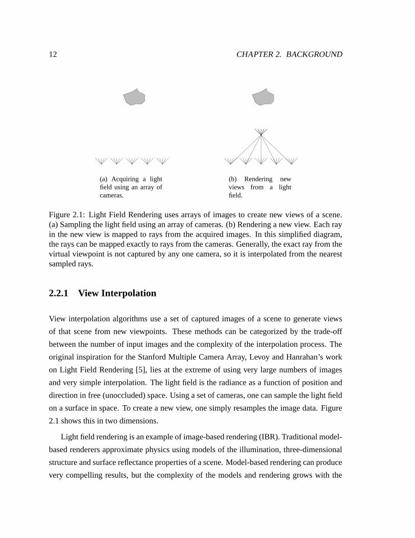
(a) Acquiring a lightfield using an array ofcameras.
(b) Rendering newviews from a lightfield.
Figure 2.1: Light Field Rendering uses arrays of images to create new views of a scene.(a) Sampling the light field using an array of cameras. (b) Rendering a new view. Each rayin the new view is mapped to rays from the acquired images. In this simplified diagram,the rays can be mapped exactly to rays from the cameras. Generally, the exact ray from thevirtual viewpoint is not captured by any one camera, so it is interpolated from the nearestsampled rays.
2.2.1 View Interpolation
View interpolation algorithms use a set of captured images of a scene to generate views
of that scene from new viewpoints. These methods can be categorized by the trade-off
between the number of input images and the complexity of the interpolation process. The
original inspiration for the Stanford Multiple Camera Array, Levoy and Hanrahan’s work
on Light Field Rendering [5], lies at the extreme of using verylarge numbers of images
and very simple interpolation. The light field is the radiance as a function of position and
direction in free (unoccluded) space. Using a set of cameras, one can sample the light field
on a surface in space. To create a new view, one simply resamples the image data. Figure
2.1 shows this in two dimensions.
Light field rendering is an example of image-based rendering(IBR). Traditional model-
based renderers approximate physics using models of the illumination, three-dimensional
structure and surface reflectance properties of a scene. Model-based rendering can produce
very compelling results, but the complexity of the models and rendering grows with the

2.2. VIEW INTERPOLATION AND HIGH-X IMAGING 13
complexity of the scene, and accurately modeling real scenes can be very difficult. Image-
based rendering, on the other hand, uses real or pre-rendered images to circumvent many of
these challenges. Chen and Williams used a set of views with precomputed correspondence
maps to quickly render novel views using image morphs [18]. Their method has a rendering
time independent of scene complexity but requires a correspondence map and has trouble
filling holes when occluded parts of the scene become visible.
Light field rendering uses no correspondence maps or explicit 3D scene models. As
described earlier, new views are generated by combining andresampling the input images.
Although rendering light fields is relatively simple, acquiring them can be very challeng-
ing. Light fields typically use over a thousand input images.The original light field work
required over four hours to capture a light field of a static scene using a single translating
camera. For dynamic scenes, one must use a camera array–the scene will not hold still
while a camera is translated to each view position. Light field rendering requires many
very closely spaced images to prevent aliasing artifacts inthe interpolated views. Ideally
the camera spacing would be equal to the aperture size of eachcamera, but practically,
this is impossible. Dynamic scenes require not only multiple cameras, but also methods to
reduce the number of required input views.
The Virtualized Reality [9] work of Rander et al. uses fewer images at the expense of
increasing rendering complexity. They surround their viewing volume with cameras and
then infer the three-dimensional structure of the scene using disparity estimation or voxel
carving methods [19, 20]. Essentially, they are combining model-based and image-based
rendering. They infer a model for the scene geometry, but compute colors by resampling
the images based on the geometric model. Matusik et al. presented another view interpo-
lation method, Image Based Visual Hulls [21], that uses silhouettes from multiple views to
generate approximate structural models of foreground objects. Although these methods use
fewer, more widely separated cameras than Light Field Rendering, inferring structure using
multiple cameras is still an unsolved vision problem and leads to artifacts in the generated
views.
How should a video camera array be designed to allow experiments across this range
of view interpolation methods? At the very least, it should store all of the data from all
cameras for reasonable length videos. At video rates (30fps), scene motion, and hence the
14 CHAPTER 2. BACKGROUND
image motion from frame to frame, can be quite significant. Most methods for inferring
3D scene structure assume a rigid scene. For an array of videocameras, this condition will
only hold if the cameras are synchronized to expose at the same time. For pure image-based
methods like Light Field Rendering, unsynchronized cameraswill result in ghost images.
Light Field Rendering requires many tightly packed cameras,but Virtualized Reality and
Image Based Visual Hulls use more widely separated cameras, so clearly a flexible camera
array should support both configurations. Finally, all of these applications assume that the
cameras can be calibrated geometrically and radiometrically.
2.2.2 High-X Imaging
High-X imaging combines many single-center-of-projection images to extend imaging per-
formance. To shed light on camera array design requirementsfor this space, I will now enu-
merate several possible high-X dimensions, discuss prior work in these areas and consider
how we might implement some of them using a large array of cameras.
High-X Imaging Dimensions
High Resolution. Images taken from a single camera rotating about its opticalcenter can
be combined to create high-resolution, wide field-of-view (FOV) panoramic image mosaics
[4]. For dynamic scenes, we must capture all of the data simultaneously. Imaging Solutions
Group of New York, Inc, offers a “quad HDTV” 30 frame-per-second video camera with a
3840 x 2160 pixel image sensor. At 8.3 megapixels per image, this is the highest resolution
video camera available. This resolution could be surpassedwith a 6 x 5 array of VGA
(640 x 480 pixel) cameras with abutting fields of view. Many companies and researchers
have already devised multi-camera systems for generating video mosaics of dynamic scenes
[22]. Most pack the cameras as closely together as possible to approximate a SCOP system,
but some use optical systems to ensure that the camera centers of projection are actually
coincident. As the number of cameras grow, these optical systems become less practical.
If the goal is just wide field of view or panoramic imaging, butnot necessarily high
resolution, then a single camera can be sufficient. For example, the Omnicamera created
by Nayar uses a parabolic mirror to image a hemispherical field of view [23]. Two such

2.2. VIEW INTERPOLATION AND HIGH-X IMAGING 15
cameras placed back-to-back form an omnidirectional camera.
Low Noise. It is well known that averaging many images of the same scene reduces image
noise (measured by the standard deviation from the expectedvalue) by the square root of
the number of images, assuming the noise is zero-mean and uncorrelated between images.
Using an array of 100 cameras in SCOP mode, we should be able to reduce image noise by
a factor of 10.
Super-Resolution. It is possible to generate a higher resolution image from a set of dis-
placed low-resolution images if one can measure the camera’s point spread function and
register the low-resolution images to sub-pixel accuracy [24]. We could attempt this with
an array of cameras. Unfortunately, super-resolution is fundamentally limited to less than
a two-fold increase in resolution, and the benefits of more input images drops off rapidly
[25, 26], so abutting fields of view is generally a better solution for increasing image res-
olution. On the other hand, many of the high-X methods listedhere use cameras with
completely overlapping fields of view, and we should be able to achieve a modest resolu-
tion gain with these methods.
Multi-Resolution Video. Multi-resolution video allows high-resolution (spatially or tem-
porally) insets within a larger lower-resolution video [27]. Using an array of cameras with
varying fields of view, we could image a dynamic scene at multiple resolutions. One use
of this would be to provide high-resolution foveal insets within a low-resolution panorama.
Another would be to circumvent the limits of traditional super-resolution. Information
from high-resolution images can be used to increase resolution of a similar low-resolution
image using texture synthesis [28], image alignment [29], or recognition-based priors [26].
In our case, we would use cameras with narrower fields of view to capture representative
portions of the scene in higher resolution. Another versionof this would be to combine
a high-speed, low-resolution video with a low-speed, high-resolution video (both captured
using high-X techniques) to create a single video with higher frame rate and resolution.
16 CHAPTER 2. BACKGROUND
High Dynamic Range. Natural scenes often have dynamic ranges (the ratio of brightest
to darkest intensity values) that far exceed the dynamic range of photographic negative film
or the image sensors in consumer digital cameras. Areas of a scene that are too bright
saturate the film or sensor and look uniformly white, with no detail. Regions that are too
dark can be either be drowned out by noise in the sensor or simply not detected due to
the sensitivity limit of the camera. Any given exposure onlycaptures a portion of the total
dynamic range of the scene. Mann and Picard [2], and Debevec and Malik [3] show ways to
combine multiple images of a still scene taken with different known exposure settings into
one high dynamic range image. Using an array of cameras with varying aperture settings,
exposure durations, or neutral density filters, we could extend this idea to dynamic scenes.
High Spectral Sensitivity. Humans have trichromatic vision, meaning that any incident
light can be visually matched using combinations of just three fixed lights with different
spectral power distributions. This is why color cameras measure three values, roughly
corresponding to red, green and blue. Multi-spectral images sample the visible spectrum
more finely. Schechner and Nayar attached a spatially varying spectral filter to a rotating
monochrome camera to create multi-spectral mosaics of still scenes. As they rotate their
camera about its center of projection, points in the scene are imaged through different
regions of the filter, corresponding to different portions of the visible spectrum. After
registering their sequence of images, they create images with much finer spectral resolution
than the three typical RGB bands. Using an array of cameras with different band-pass
spectral filters, we could create multi-spectral videos of dynamic scenes.
High Depth of Field. Conventional optical systems can only focus well on objects within
a limited range of depths. This range is called the depth of field of the cameras, and it
is determined primarily by the distance at which the camera is focused (depth of field
increases with distance) and the diameter of the camera aperture (larger apertures result in
a smaller depth of field). For static scenes, depth of field canbe extended using several
images with different focal depths and selecting, for each pixel, the value from the image
in which is is best focused [30]. The same principle could be applied to a SCOP camera
array. One challenge is that depth of field is most limited close to the camera, where the
2.2. VIEW INTERPOLATION AND HIGH-X IMAGING 17
SCOP approximation for a camera array breaks down. Successfully applying this method
would require either an optical system that ensures a commoncenter of projection for the
cameras or sophisticated image alignment algorithms.
Large Aperture. In chapter 4, I describe how we use our camera array as a large syn-
thetic aperture camera. I have already noted that the very narrow depth of field caused
by large camera apertures can be exploited to look beyond partially occluding foreground
objects, blurring them so as to make them invisible. In low-light conditions, large apertures
are also useful because they admit more light, increasing the signal-to-noise ratio of the
imaging system. This is the one high-X application that is deliberately not single-center-
of-projection. Instead, it relies on slightly different centers of projection for all cameras.
High Speed. Typical commercial high-speed cameras run at frame rates ofhundreds to
thousands of frames per second, and high-speed video cameras have been demonstrated
running as high as one million frames per second [31]. As frame rates increase for a fixed
resolution, continuous streaming becomes impossible, limiting users to short recording du-
rations. Chapter 5 discusses in detail high-speed video capture using the Stanford Multiple
Camera Array. Here, I will just reiterate that we use many sensors with evenly staggered
triggers, and that parallel capture (and compression) permits continuous streaming.
Camera Array Design for High-X Imaging
A camera array for High-X imaging should allow all of the fine control over various camera
parameters required by traditional single-camera applications but also address the issues
that arise when those methods are extended to multiple cameras. For multiple-camera
high-x applications, the input images should generally be views of the same scene at the
same time from the same position, from cameras that respond identically to and capture
the same range of intensities. Thus, the cameras should be designed to be tightly packed
to approximate a single center of projection, synchronizedto trigger simultaneously, and
configured with wholly overlapping fields of view. Furthermore, we must set their exposure
times and color gains and offsets to capture the same range ofintensities. None of these

18 CHAPTER 2. BACKGROUND
steps can be done perfectly, and the cameras will always vary, so we will need to calibrate
geometrically and radiometrically to correct residual errors.
For most high-x applications, at least one parameter must beallowed to vary, so a cam-
era array should also support as much flexibility and controlover as many camera properties
as possible. In fact, we find reason to break every guideline listed above. For example, to
capture high dynamic range images, we configure the cameras to sense varying intensity
ranges. Synthetic aperture photography explicitly defies the SCOP model to capture multi-
ple viewpoints. To use the array for high-resolution capture, we must abut the fields of view
instead of overlapping them. Finally, high-speed imaging relies on precisely staggered, not
simultaneous, trigger times. Flexibility is essential.
2.3 Inexpensive Image Sensing
Nearly all of the applications and arrays presented so far used relatively high quality cam-
eras. How will these applications map to arrays of inexpensive image sensors? Cheap
image sensors are optimized to produce pictures to be viewedby humans, not by comput-
ers. This section discusses how cheap sensors exploit our perceptual insensitivity to certain
types of imaging errors and the implications of these optimizations for high performance
imaging.
2.3.1 Varying Color Responses
The vast majority of image sensors are used in single-cameraapplications where the goal
is to produce pleasing pictures, and human color perceptionsenses relative differences
between colors, not absolute colors [32]. For these reasons, manufacturers of image sensors
are primarily concerned with only the relative accuracy of their sensors. Auto-gain and
auto-exposure ensure the image is exposed properly, and white balancing algorithms adjust
color gains and the output image to fit some assumption of the color content of the scene.
These feedback loops automatically compensate for any variations in the sensor response
while they account for external factors like the illumination. Without a reference, it is often
difficult for us to judge the fidelity of the color reproduction.

2.3. INEXPENSIVE IMAGE SENSING 19
For IBR and high-X applications that use just one camera to capture multiple images,
the actual shape of the sensor’s response curve (i.e. digital pixel value as a function of
incident illumination), and its response to light of different wavelengths, are unimportant
as long as they are constant and the response is monotonic. With multiple cameras, differ-
ences in the absolute response of each camera become relative differences between their
images. These differences can be disastrous if the images are directly compared, either by a
human or an algorithm. A panoramic mosaic stitched togetherfrom cameras with different
responses will have an obviously incorrect appearance, even if each region viewed indi-
vidually looks acceptable. Methods that try to establish corresponding scene points in two
images often assume brightness constancy, meaning that a scene point appears the same
in all images of it. Correcting the color differences betweencameras is essential for these
applications.
Because so few end users care about color matching between sensors, variations in color
response between image sensors are poorly documented. In practice, these differences can
be quite large. In chapter 5, I will show that for the image sensors in the array, the color
responses of 100 chips set to the same default gain and exposure values varies quite widely.
2.3.2 Color Imaging and Color Filter Arrays
One key result of color science is that because the human eye has only three different
types of cones for detecting color, it is possible to represent all perceptually discernible
colors with just three primaries, each having linearly independent spectral power distribu-
tions. Practically, this means that color image sensors only need to measure the incident
illumination using detectors with three appropriately chosen spectral responses instead of
measuring the entire spectra. Typically, these responses correspond roughly to what we per-
ceive as red, green and blue. Each pixel in an image sensor makes only one measurement,
so some method must be devised to measure three color components.
High-end color digital cameras commonly use three image sensors and special optics
that send the incident red light to one sensor, the green to another, and the blue to a third.
This measures three color values at each pixel, but the extraimage sensors and precisely
aligned optics increase the total cost of camera.
20 CHAPTER 2. BACKGROUND
G B
GR
G B
GR
G B
GR
G B
GR
G B
GR
G B
GR
G B
GR
G B
GR
G B
GR
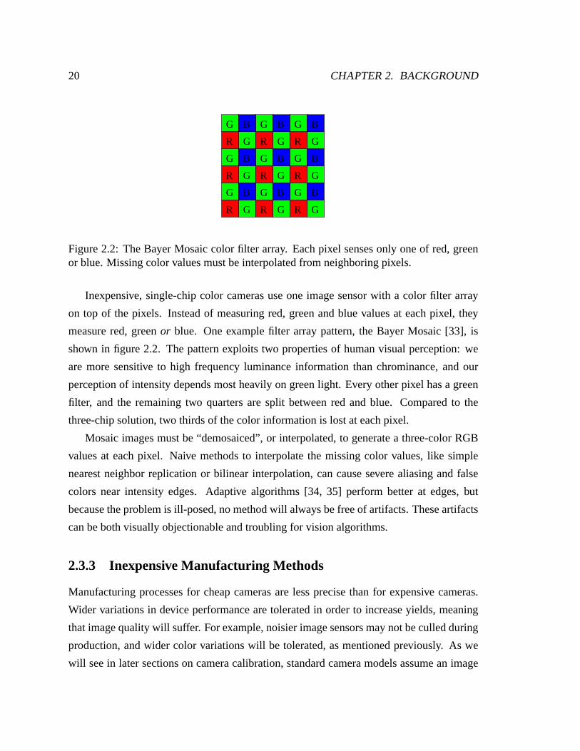
Figure 2.2: The Bayer Mosaic color filter array. Each pixel senses only one of red, greenor blue. Missing color values must be interpolated from neighboring pixels.
Inexpensive, single-chip color cameras use one image sensor with a color filter array
on top of the pixels. Instead of measuring red, green and bluevalues at each pixel, they
measure red, greenor blue. One example filter array pattern, the Bayer Mosaic [33],is
shown in figure 2.2. The pattern exploits two properties of human visual perception: we
are more sensitive to high frequency luminance informationthan chrominance, and our
perception of intensity depends most heavily on green light. Every other pixel has a green
filter, and the remaining two quarters are split between red and blue. Compared to the
three-chip solution, two thirds of the color information islost at each pixel.
Mosaic images must be “demosaiced”, or interpolated, to generate a three-color RGB
values at each pixel. Naive methods to interpolate the missing color values, like simple
nearest neighbor replication or bilinear interpolation, can cause severe aliasing and false
colors near intensity edges. Adaptive algorithms [34, 35] perform better at edges, but
because the problem is ill-posed, no method will always be free of artifacts. These artifacts
can be both visually objectionable and troubling for visionalgorithms.
2.3.3 Inexpensive Manufacturing Methods
Manufacturing processes for cheap cameras are less precisethan for expensive cameras.
Wider variations in device performance are tolerated in order to increase yields, meaning
that image quality will suffer. For example, noisier image sensors may not be culled during
production, and wider color variations will be tolerated, as mentioned previously. As we
will see in later sections on camera calibration, standard camera models assume an image
2.3. INEXPENSIVE IMAGE SENSING 21
plane that is perpendicular to the lens’ optical axis. On inexpensive sensors, however, the
dies may be tilted and rotated on the package, violating thatmodel.
The optical systems for cheap cameras are also of lower quality. Although glass lenses
produce better images, very cheap cameras use plastic lenses or hybrid glass-plastic lenses
instead. Furthermore, avoiding artifacts such as spherical and chromatic aberration requires
multiple lens elements, which will be less precisely placedin a cheap sensor. Less precise
placement will cause distortions in the image and more inconsistencies between the camera
and commonly used models. Finally, high-quality lenses provide adjustments to control the
aperture size and focal length, but in inexpensive lenses, these quantities are fixed.
In the next chapter, I describe the Stanford Multiple Camera Array and the design de-
cisions I made in its implementation. One goal for the systemwas to use cheaper, lower-
quality components and compensate for their drawbacks in software where possible. Thus,
we chose fixed-focus, fixed-aperture lenses for their affordability. Similarly, the decreased
cost and complexity of designing single-chip color camerasoutweighed the disadvantages
of subsampled color due to the Bayer Mosaic. These are two examples of the many trade-
offs involved in the design of the array.
22 CHAPTER 2. BACKGROUND

Chapter 3
The Stanford Multiple Camera Array
The broad range of applications for camera arrays combined with the promise of inex-
pensive, easy to use, smart cameras and plentiful processing motivated exploration of the
potential of large arrays of cheap cameras. In this chapter,I present a scalable, general-
purpose camera array that captures video continuously fromover 100 precisely-timed cam-
eras to just four PCs. Instead of using off-the-shelf cameras, I designed custom ones, lever-
aging existing technologies for our particular goals. I chose CMOS image sensors with
purely digital interfaces so I could easily control the gain, exposure and timing for all the
cameras. MPEG2 video compression at each camera reduces thedata bandwidth of the sys-
tem by an order of magnitude. High-speed IEEE1394 interfaces make the system modular
and easily scalable. Later chapters show the array being used in a variety of configurations
for several different applications. Here, I explain the technology that makes this possible.
3.1 Goals and Specifications
The Stanford Multiple Camera Array is intended to be a flexibleresearch tool for exploring
applications of large numbers of cameras. At the very least,I wanted to be able to imple-
ment IBR and High-X methods similar to those described in the previous chapter. This
requires large numbers of cameras with precise timing control, the ability to tightly pack or
widely space the cameras, and low-level control over the camera parameters. For the de-
vice to be as general as possible, it should capture and storeall data from all the cameras. I
23
24 CHAPTER 3. THE STANFORD MULTIPLE CAMERA ARRAY
also wanted the architecture to be modular and easily scalable so it could span applications
requiring anywhere from a handful to over one hundred cameras. One implication of this
scalability was that even though the array might have over one hundred cameras, it should
use far fewer than one hundred PCs to run it, ideally just a handful. Finally, reconfiguring
the array for different applications should not be a significant obstacle to testing out new
ideas.
To begin quantifying the specifications of our array, I started with the same video reso-
lution and frame rate as the 3D Room: 640x480 pixel, 30fps progressive scan video. 30fps
is generally regarded as the minimum frame rate for real-time video, and 640x480 is suit-
able for full-screen video. To demonstrate scalability, I aimed for a total of 128 cameras. To
record entire performances, I set a goal of recording video sequences at least ten minutes
long.
No off-the-shelf solution could meet these design goals. The cameras had to be tiny and
provide a means to synchronize to each other. I also wanted tobe able to control and stream
video from at least 30 of the cameras to a single PC. There simply were no cameras on the
market that satisfied these needs. By building custom cameras, I was able to explicitly add
the features I needed and leave room to expand the abilities of the cameras in the future.
3.2 Design Overview
The Stanford Multiple Camera array streams video from many CMOS image sensors over
IEEE1394 buses to a small number of PCs. Pixel data from each sensor flows to an FPGA
that routes it to local DRAM memory for storage or to an IEEE1394 chipset for transmis-
sion to a PC. The FPGA can optionally perform low-level image processing or pass the
data through an MPEG encoder before sending it to the 1394 chipset. An embedded mi-
croprocessor manages the components in the camera and communicates with the host PCs
over IEEE1394. In this section, I describe the major technologies used in the array: CMOS
image sensors, MPEG video compression, and IEEE1394 communication.

3.2. DESIGN OVERVIEW 25
3.2.1 CMOS Image Sensors
One of the earliest decisions for the array was to use CMOS instead of CCD image sensors.
CCDs are fully analog devices, requiring more careful design,supporting electronics to
digitize their output, and often multiple supply voltages or clocks. CMOS image sensors,
on the other hand, generally run off standard logic power supplies, can output 8-or 16 bit-
digital video, and can connect directly to other logic chips. Sensor gains, offsets, exposure
time, gamma curves and more can often be programmed into registers on the chip using
standard serial interfaces. Some CMOS sensors even have digital horizontal and vertical
sync inputs for synchronization. These digital interfacesmake the design simpler and more
powerful. Immediate practical concerns aside, because digital logic can be integrated on
the same chip, CMOS sensors offer the potential of evolving into “smart” cameras, and it
seemed sensible to base our design on that technology.
The many advantages of using CMOS sensors come with a price. CMOS sensors are
inherently noisier [36] and less sensitive than their CCD counterparts. For these reasons,
CCD sensors are still the technology of choice for most high performance applications
[37]. I decided to sacrifice potential gains in image qualityin exchange for a much more
tractable design and added functionality.
3.2.2 MPEG2 Video Compression
The main goals for the array are somewhat contradictory: it should store all of the video
from all of our cameras for entire performances, but also scale easily to over one hundred
cameras using just a handful of PCs. An array of 128, 640x480 pixel, 30fps, one byte per
pixel, Bayer Mosaic video cameras generates over 1GB/sec of raw data, roughly twenty
times the maximum sustained throughput for today’s commodity hard drives and peripheral
interfaces. The creators of the 3D Room attacked this problemby storing raw video from
cameras to main memory in PCs. With 49 cameras and 17 PCs with 512MB of main
memory, they were able to store nearly 9 seconds of video. To capture much longer datasets
using far fewer PCs, I took a different approach: compressingthe video.
One video compression option for the array was DCT-based intra-frame video encoding
26 CHAPTER 3. THE STANFORD MULTIPLE CAMERA ARRAY
like DV. Commercial DV compression hardware was either too costly are simply unavail-
able when I built the array. MPEG2 uses motion prediction to encode video with a much
higher compression ratio, and Sony, one of the early sponsors of this work, offered their
MPEG2 compression chips at a reasonable price. A relativelystandard 5Mb/s bitstream
for 640x480, 30fps video translates into a compression ratio of 14:1, and at 4Mb/s, the
default for the Sony encoder, this results in 17.5:1 compression. 128 cameras producing
5Mb/s bitstreams create 80MB/s of data, back in the ballpark of bandwidths we might
hope to get from standard peripheral buses and striped hard drives. The disadvantage of
MPEG compression is that it is lossy, meaning that one cannotexactly reproduce the orig-
inal uncompressed video. I opted to use it anyway, but in order to investigate the effects of
compression artifacts I designed the cameras to simultaneously store brief segments of raw
video to local memory while streaming compressed video. This lets one compare MPEG2
compressed video with raw video for array applications.
3.2.3 IEEE1394
The last piece of the array design was a high bandwidth, flexible and scalable means to
connect cameras to the host PCs. I chose the IEEE1394 High Performance Serial Bus [38],
which has several properties that make it ideal for this purpose. It guarantees a default
bandwidth of 40MB/s for “isochronous” transfers, data that is sent at a constant rate. This
is perfect for streaming video, and indeed many digital video cameras connect to PCs via
IEEE1394 (also known as FireWireR© and i-LinkR©). IEEE1394 is also well suited for a
modular, scalable design because it allows up to 63 devices on each bus and supports plug
and play. As long as the bandwidth limit for a given bus is not exceeded, one can add or
remove cameras at will and the bus will automatically detectand enumerate each device.
Another benefit of IEEE1394 is the cabling environment. IEEE1394 cables can be up to
4.5m long, and an entire bus can span over 250m, good news if wewant to space our
cameras very widely apart, say on the side of a building.
The combination of MPEG2 and IEEE1394 creates a natural “sweet spot” for a large
camera array design. A full bus can hold 63 devices; if we set aside one device for a
host PC, it can still support up to 62 cameras. 62 MPEG2 video streams at 5Mb/s add
3.3. SYSTEM ARCHITECTURE 27
up to 310Mb/s of data, just within the default 320Mb/s limit of the bus. 320Mb/s is also
well within the bandwidth of two software striped IDE hard drives, so this setup means
I could reasonably hope to require only one PC per 60 cameras in our architecture. For
reasons I will discuss later, the current system supports only 25 cameras per PC with 4Mb/s
bitstreams, but a more sophisticated implementation should be able to approach a full set
of 62 cameras per bus.
3.3 System Architecture
To be scalable and flexible, the system architecture had to not only meet the video capture
requirements but also easily support changes in the number of cameras, their functionality,
and their placement. Each camera is a separate IEEE1394 device, so adding or removing
cameras is simple. I embedded a microprocessor to manage theIEEE1394 interface, the
image sensor and the MPEG encoder. Accompanying the processor is an EEPROM for a
simple boot loader and DRAM memory for storing image data and an executable down-
loaded over the IEEE1394 bus. The image sensor, MPEG encoderand IEEE1394 chips all
have different data interfaces, so I added an FPGA for glue logic. Anticipating that I might
want to add low-level image processing to each camera, I useda higher-performance FPGA
than necessary and connected it to extra SRAM and SDRAM memory.Because the timing
requirements for the array were stricter than could be achieved using IEEE1394 commu-
nication, especially with multiple PCs, I added CAT5 cables toeach camera to receive the
clock and trigger signals and propagate them to two other nodes. All of these chips and
connections take up more board area than would fit on a tiny, densely-packable camera, so
I divided the cameras into two pieces: tiny camera “tiles” containing just the image sensor
and optics, and larger boards with the rest of the electronics.
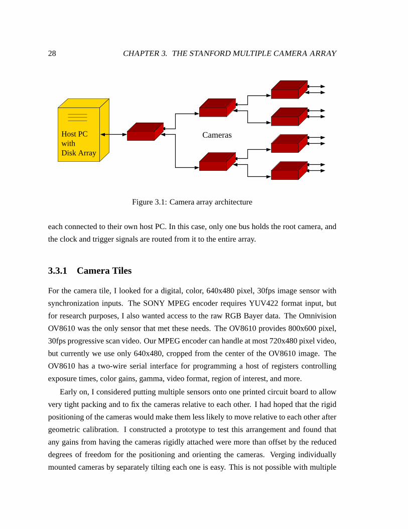
Figure 3.1 shows how the cameras are connected to each other and to the host PCs using
a binary tree topology. One camera board is designated as theroot camera. It generates
clocks and triggers that are propagated to all of the other cameras in the array. The root
is connected via IEEE1394 to the host PC and two children. TheCAT5 cables mirror the
IEEE1394 connections between the root camera and the rest ofthe array. When camera
numbers or bandwidth exceed the maximum for one IEEE1394 bus, we use multiple buses,
28 CHAPTER 3. THE STANFORD MULTIPLE CAMERA ARRAY
CameraswithHost PC
Disk Array
Figure 3.1: Camera array architecture
each connected to their own host PC. In this case, only one bus holds the root camera, and
the clock and trigger signals are routed from it to the entirearray.
3.3.1 Camera Tiles
For the camera tile, I looked for a digital, color, 640x480 pixel, 30fps image sensor with
synchronization inputs. The SONY MPEG encoder requires YUV422 format input, but
for research purposes, I also wanted access to the raw RGB Bayerdata. The Omnivision
OV8610 was the only sensor that met these needs. The OV8610 provides 800x600 pixel,
30fps progressive scan video. Our MPEG encoder can handle atmost 720x480 pixel video,
but currently we use only 640x480, cropped from the center ofthe OV8610 image. The
OV8610 has a two-wire serial interface for programming a host of registers controlling
exposure times, color gains, gamma, video format, region ofinterest, and more.
Early on, I considered putting multiple sensors onto one printed circuit board to allow
very tight packing and to fix the cameras relative to each other. I had hoped that the rigid
positioning of the cameras would make them less likely to move relative to each other after
geometric calibration. I constructed a prototype to test this arrangement and found that
any gains from having the cameras rigidly attached were morethan offset by the reduced
degrees of freedom for the positioning and orienting the cameras. Verging individually
mounted cameras by separately tilting each one is easy. Thisis not possible with multiple

3.3. SYSTEM ARCHITECTURE 29
Figure 3.2: A camera tile.
sensors on the same flat printed circuit board without expensive optics. Manufacturing vari-
ations for inexpensive lenses and uncertainty in the placement of image sensor of a printed
circuit board also cause large variations in the orientation of the cameras. The orientations
even change as the lenses are rotated for proper focus. Correcting these variations requires
individual mechanical alignment for each camera.
The final camera tile is shown in figure 3.2. Two meter long ribbon cables carry video,
synchronization signals, control signals, and power between the tile and the processing
board. The tile uses M12x0.5 lenses and lens mounts, a commonsize for small board cam-
eras (M12 refers to the thread pitch, and 0.5 to the radius of the lens barrel in centimeters).
The lens shown is a Sunex DSL841B. These lenses are fixed focus and have no aperture
settings. For indoor applications, one often wants a large working volume viewable from
all cameras, so I chose a lens with a small focal length, smallaperture and large depth of
field. The DSL841B has a fixed focal length of 6.1mm, a fixed aperture F/# of 2.6, and a di-
agonal field of view of 57◦. For outdoor experiments and applications that require narrow
field of view cameras, we use Marshall Electronics V-4350-2.5 lenses with a fixed focal
length of 50mm, 6◦ diagonal field of view, and F/# of 2.5. Both sets of optics include an
IR filter.
The camera tiles measure only 30mm on a side, so they can be packed very tightly.
They are mounted to supports using three spring-loaded screws. These screws not only
hold the cameras in place but also let one fine-tune their orientations. The mounts let us

30 CHAPTER 3. THE STANFORD MULTIPLE CAMERA ARRAY
Figure 3.3: 52 cameras on a laser-cut acrylic mount.
correct the direction of the camera’s optical axis (which way it points), but not rotations
around the axis caused by a slightly rotated image sensor.
The purpose of the mounting system is not to provide precise alignment, but to ensure
that the cameras have enough flexibility so we align them roughly according to our needs,
then correct for variations later in software. Being able to verge the cameras sufficiently
is critical for maintaining as large a working volume as possible, or even ensuring that all
cameras see at least one common point. Image rotations are less important because they
do not affect the working volume as severely, but as we will see later, they do limit the
performance of our high speed video capture method.
For densely packed configurations such as in figure 3.3, the cameras are mounted di-
rectly to a piece of laser cut acrylic with precisely spaced holes for cables and screws. This
fixes the possible camera positions but provides very regular spacing. Laser cutting plas-
tic mounts is quick and inexpensive, making it useful for prototyping and experimenting.
For more widely spaced arrangements, the cameras are connected to 80/20 mounts using
a small laser-cut plastic adaptor. 80/20 manufactures whatthey call the “Industrial Erec-
tor Set”R©, a T-slotted aluminum framing system. With the 80/20 system, we can create
different camera arrangements to suit our needs. Figure 3.4below shows some of the
arrangements built with this system.

3.3. SYSTEM ARCHITECTURE 31
Figure 3.4: Different array configurations using 80/20 mounts.
Figure 3.5: Camera processing board
32 CHAPTER 3. THE STANFORD MULTIPLE CAMERA ARRAY
3.3.2 Processing Boards
The processing board for each camera represents the bulk of the cost, functionality and
design effort for the camera array. The board can capture 20 frames of raw video to local
memory and stream raw or MPEG-compressed video to the host PC.Because there are
many ways to design a board for a given functionality, I will cover the functionality and
hardware choices at a high level and delve into details only for aspects of the design that
enable unique features of the array (such as the timing accuracy) or made it particularly
useful for research purposes.
Figure 3.5 shows the processing board. Each of these boards manages just one image
sensor. The major components were chosen to maximize performance at reasonable design
and manufacturing cost. The SONY CXD1922Q MPEG2 encoders were obtained at a
discount for this project. I chose a Texas Instruments chipset for the IEEE1394 interface
because they were a clear market leader at the time. These chips claim a glueless interface
to Motorola Coldfire processors, so I selected a Motorola MCF5206E processor to manage
the IEEE1394 chipset and MPEG encoder. I included 32MB of EDODRAM, the maximum
the processor supports, because this sets the limit on how much raw data each camera
can capture. An IDT72V245 8KB FIFO buffers data between the IEEE1394 streaming
interface and the rest of the board.
A Xilinx XC2S200 Spartan II FPGA along with a pair of 64Mbit SDRAMs and a pair
of 4Mbit SRAMs provides glue logic between the different chips and some low-level pro-
cessing power. FPGAs, (Field Programmable Gate Arrays), are configurable logic chips.
They do not fetch instructions like microprocessors. Instead, they are a sea of identical,
generic logic blocks with programmable functions and interconnect. A bitfile streamed
into the FPGA configures the function of each logic block and the connections between
blocks. The bitfile is specified using a behavioral language like Verilog. This specification
is more complicated than programming a processor in C for thedesigner, but is necessary
to handle non-standard data interfaces and to process videoin real-time.
Figure 3.6 shows the data flow through the processing board. To stream raw video, the
FPGA routes the incoming video straight through to the IEEE1394 chipset for isochronous
transfer back to the host PC. For MPEG2 compressed video, the sensor data is sent to
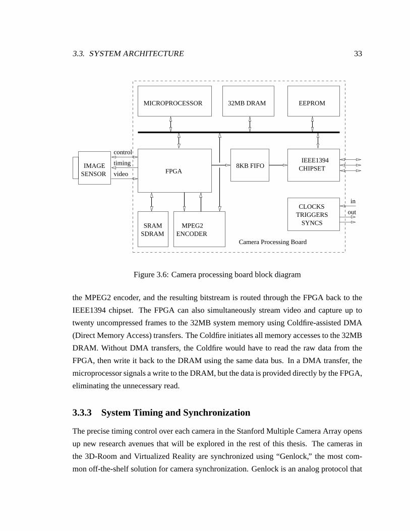
3.3. SYSTEM ARCHITECTURE 33
SENSORIMAGE
video
timing
control
in
out
Camera Processing Board
IEEE1394CHIPSET
CLOCKSTRIGGERS
SYNCS
8KB FIFO
MPEG2ENCODERSDRAM
SRAM
FPGA
MICROPROCESSOR 32MB DRAM EEPROM
Figure 3.6: Camera processing board block diagram
the MPEG2 encoder, and the resulting bitstream is routed through the FPGA back to the
IEEE1394 chipset. The FPGA can also simultaneously stream video and capture up to
twenty uncompressed frames to the 32MB system memory using Coldfire-assisted DMA
(Direct Memory Access) transfers. The Coldfire initiates allmemory accesses to the 32MB
DRAM. Without DMA transfers, the Coldfire would have to read theraw data from the
FPGA, then write it back to the DRAM using the same data bus. In aDMA transfer, the
microprocessor signals a write to the DRAM, but the data is provided directly by the FPGA,
eliminating the unnecessary read.
3.3.3 System Timing and Synchronization
The precise timing control over each camera in the Stanford Multiple Camera Array opens
up new research avenues that will be explored in the rest of this thesis. The cameras in
the 3D-Room and Virtualized Reality are synchronized using “Genlock,” the most com-
mon off-the-shelf solution for camera synchronization. Genlock is an analog protocol that
34 CHAPTER 3. THE STANFORD MULTIPLE CAMERA ARRAY
provides synchronization with coincident triggers, not arbitrary timing, and is too costly
for inexpensive cameras. This is why the Dynamic Light FieldViewer, constructed of
inexpensive webcams, is not synchronized.
The Stanford Multiple Camera Array provides accurate timingwith arbitrary phase
shifts between camera triggers using the FPGAs and dedicated clock and trigger lines that
run through the entire array. The one root board in the array generates its own 27MHz
clock and sends it to two children via CAT5 cables, which then buffer the clock and send
it to two more children, and so on. The root board is identicalto the other camera boards
except for the code in one GAL and a single jumper setting. A PLL on each board uses
the system clock to generate duty-cycle corrected, 27MHz and 54MHz clocks. The MPEG
encoders require a 27MHz clock, but we run the microprocessors and FPGAs twice as fast
to maximize their performance.
The clock is not used for data transmission between boards, so delay from camera to
camera is unimportant. The shared clock only ensures that all boards are frequency-locked.
It is possible that the duty cycle degrades with each buffering of the clock, but the board
components require a 45%−55% duty cycle. This is one reason the cameras propagate a
27MHz clock, then double it on the board with a PLL. Preserving the 27MHz duty cycle is
also easier because the period is twice as long, and the PLL ensures a 50% duty cycle on the
processing boards. Propagating the system clock using a minimal depth binary tree routing
topology preserves the duty cycle by ensuring a bound of log2N hops from the root board
to any camera, as opposed to N-1 for a daisy-chained system. We also invert the sense of
the clock each time it is buffered, so systematic duty cycle offsets in the clock propagation
circuitry are roughly cancelled. In practice, this system works quite well. The maximum
depth of our tree for a 100 camera array is eight levels, and wehave tested daisy-chained
configurations with more than 16 cameras with no problems.
Frequency-locked system clocks prevent our cameras from drifting relative to each
other. The FPGAs on each board generate vertical and horizontal synchronization signals
for the image sensors and the MPEG2 encoders. The encoders actually drive the system
timing because their requirements are very exact—NTSC timing based on a 525 line-per-
image video with a 27MHz clock. The FPGAs timing units run theimage sensors and
MPEG encoders at exactly the same frame rate. With a common system clock, this means
3.3. SYSTEM ARCHITECTURE 35
that all the sensors and encoders run at exactly the same frequency.
Synchronization is more than just preventing frequency drift. We also need to set the
relative timing of the cameras’ exposures and the frame on which the cameras start and stop
capturing video. The timing of IEEE1394 transfers, especially from multiple networked
PCs, is simply too uncertain for the accuracy we need in our system, so I put that control
directly into our hardware. The same CAT5 cables that carry the clock transmit global
triggers from the root board to the rest of the array. These signals route directly to the
FPGAs on the boards. They control the initial synchronization or staggering of the sensor
shutter timing and the frame-accurate start of all video streaming or snapshots.
Video timing initialization is a good example of how to execute timing-sensitive com-
mands for the camera array. The FPGAs use two video counters to drive the vertical and
horizontal inputs of the image sensors and MPEG2 encoders. Thepixel counter rolls over
when it reaches the number of pixels in a line, causing theline counter to increment. The
line counter rolls over at 525 lines, signaling a new frame. Once these counters have been
initialized, they run without drift across the entire arraybecause of the common system
clock. The reset values for the line counters is a programmable register on the FPGA,
accessible via an IEEE1394 command to the board.
To set up arbitrary time shifts between cameras, we program different values into the
line counter reset registers, send a command which instructs the boards to reset their coun-
ters on the next rising trigger signal, and then tell the rootboard to assert the trigger. All
of the setup for all boards is done using IEEE1394 reads and writes, but the order to reset
their timers, which must be executed at the same time by all cameras, is sent just to the root
board. The root board then asserts the trigger signal for theentire array. The inaccuracy of
the camera synchronization is limited to the electrical delay propagating the trigger to all
of the boards. For the 100-camera array, this is less than 150ns, or roughly the time to scan
out four pixels from the image sensor.
3.3.4 Developer Interface to the Boards via IEEE1394
A flexible mounting system and low-level camera control makeit easy to experiment with
different applications, but we also need a development environment that facilitates adding
36 CHAPTER 3. THE STANFORD MULTIPLE CAMERA ARRAY
new features to the cameras. I took advantage of the IEEE1394bus to make prototyping
quick and easy. After power-up or a board reset, the Coldfire executes simple boot code
which configures the microprocessor memory and the IEEE1394interface. The host PC
then downloads FPGA bitfiles and a more sophisticated Coldfireexecutable from the PC
via IEEE1394. Adding new camera features is just a matter of compiling these new files
and does not require modifications to the physical hardware (i.e. programming GALs or
boot ROMs). This is critical for an array of 100 cameras.
A simple bootloader and downloadable executables and bitfiles makes iterating design
changes easy. Other goals for the design environment were toimplement as much as pos-
sible on the host PC using a familiar C development environment, keep the downloaded
executable simple, and expose as much of the camera state as possible to the user. Once the
final executable has been downloaded, the important state ineach camera is mapped into its
IEEE1394 address space. Using standard IEEE1394 reads and writes, one can access the
full 32MB of DRAM attached to the processor, all of the controlregisters in the MPEG2
encoder and IEEE1394 chipset, configuration registers programmed into the FPGA, and
control registers for the cameras themselves. This keeps the developer API for the array
simple—just IEEE1394 reads and writes—and makes it easy to track the state of the board
(what has been programmed into registers in the FPGA, image sensor, MPEG encoder)
from the host PC application.
3.3.5 Image Processing on the FPGA
Raw image data from the cameras almost always need to be processed before they can be
used. With this in mind, I designed the cameras for reasonable cost with as powerful an
FPGA and as much associated memory as I could. As one example of the potential of the
FPGA, we have implemented Bayer demosaicing of the raw sensordata using the Adaptive
Color Plane Interpolation algorithm of [39]. This method needs access to five adjacent
lines of raw image data, meaning the FPGA must buffer four lines of the image. Rather
than use the external memory, we use built-in BlockRAMs on the Spartan-II. These RAMs
can be used for FIFOs with up to 511 entries, so for this exercise we processed only 510-
pixel-wide images. We have also implemented arbitrary geometric warps for color images
3.3. SYSTEM ARCHITECTURE 37
using lookup tables with eighth-pixel accurate coordinates and bilinear interpolation. We
currently use this for keystone corrections so we can view live synthetic aperture video.
3.3.6 Limits due to IEEE1394 Arbitration
The maximum isochronous (streaming) data transfer rate forIEEE1394 is 320Mb/s. The
standard method for streaming data from many different IEEE1394 devices is to assign
each one a different isochronous channel number and a fixed portion of the bandwidth
in each 1394 cycle, but this turns out to be a poor strategy. One device streaming data
can achieve the maximum rate, but with many nodes, arbitration overhead will reduce the
maximum bandwidth. Devices must arbitrate before every isochronous packet is sent, and
arbitration takes longer with more nodes because signals must propagate from all nodes up
to the root and then back. Moreover, each IEEE1394 packet also has an overhead of three
quadlets (four bytes each) to describe the packet (data length, isochronous channel number,
data correction, and so on).
For an MPEG data rate of 4Mb/s (the default for our encoders),each camera must trans-
fer 66 bytes every 125us isochronous cycle. IEEE1394 packetlengths must be multiples of
four, meaning each camera must be configured to stream 68-byte packets. Adding twelve
bytes for packet overhead produces an 80-byte packet. At most, 51, 80-byte packets would
fit in the maximum of 4096 bytes per cycle. After arbitration overhead, we have found that
we can stream only 26, 4Mb/s cameras reliably. We have verified with an IEEE1394 bus
snooper that arbitration overhead is indeed the culprit preventing more packets on the bus.
Streaming such small packets each cycle from every camera produces a data file on the
host PC that is very fragmented and thus hard to process. Programs must scan through the
data 80 bytes at a time to look for data from a specific camera. To fix this difficulty and the
overhead issues, we attempted to implement an isochronous transfer scheme in which each
camera sends a full 4096-byte isochronous packet every N cycles. Each camera counts
isochronous cycles using the cycle done interrupt from the IEEE1394 chipset. Access to
the bus passes round-robin through the array, and each camera is responsible for attempting
to send data only on its dedicated cycle.

38 CHAPTER 3. THE STANFORD MULTIPLE CAMERA ARRAY
We cannot implement this scheme with 4KB packets because we have a one-cycle un-
certainty in our control over the IEEE1394 bus. Instead, we set the cameras to transmit a
2KB packet on their designated cycle. If a camera is late one cycle and transmits at the
same time as its successor, the data will still fit in the cycleand no errors will occur. This
optimization makes real-time applications much easier by fragmenting the data less and
slightly increases the number of cameras we can stream simultaneously on the bus. We are
still investigating what is necessary for cycle-accurate control of the isochronous interface.
3.3.7 Host PCs
Given the limit of roughly thirty cameras per IEEE1394 bus, 100 cameras require multiple
IEEE1394 buses. At this point, we run into another limit on our data transfer bandwidth—
the 33MHz PCI bus in our computers. The IEEE1394 adaptor is a PCIdevice, and transfer-
ring data from it to our hard drives requires two PCI transfers, one from the adaptor to main
memory, and a second to the hard drives. The transfers are both DMA-assisted, but here the
role of the DMA is just to free the processor, not to reduce PCI bus bandwidth. The max-
imum theoretical bandwidth for 33MHz PCI is 133MB/sec, but themaximum sustained
data transfer rate is much less. An aggressive estimate of 80MB/s means we are limited to
one IEEE1394 bus per computer. Thus, we need one computer forevery thirty cameras.
The currentl implementation of the array with one hundred cameras uses four host PCs
which each manage a separate IEEE1394 bus. We run a copy of thearray software on each
PC using a client/server setup where the server is the PC connected to the root board of the
array. The server issues all commands for downloading executables and code, setting up
timing, programming registers on the image sensors, recording MPEG2 compressed video,
uploading stored snapshots of raw images, and so on. The onlycommand that cannot
always be run from the server is viewing live uncompressed video from the cameras—
rather than trying to send live video across the network fromPC to PC, raw video is always
viewed on the host PC for a given camera’s IEEE1394 bus. We usea DVM switch to access
all of the machines from one keyboard and monitor.
The host PCs have been optimized for our applications but are now somewhat out-of-
date. They use IEEE1394 PCI cards and striped IDE hard drives to write incoming video
3.3. SYSTEM ARCHITECTURE 39
to disk as fast as it arrives. The PCs run RedHat Linux using the experimental IEEE1394
drivers, with one modification. The IEEE1394 specification allows up to 64 isochronous
channels on a bus, but the Linux drivers currently support only four. Each camera in
our system needs its own isochronous channel, so I modified the drivers to support the
full 64 channels. Without this capability, our cameras would have to stream on the same
isochronous channel and insert the camera number into a header in every streaming packet.
More importantly, we would have to schedule the camera data transfer explicitly instead of
relying on the IEEE1394 chipsets.
3.3.8 Design Environment
The choice of operating systems and design environments canbe a matter of taste and is
not critical to the performance of our architecture. I wouldlike to briefly mention some
choices that turned out to be both inexpensive and powerful,and to acknowledge some of
the open source software tools that made our work easier. Onedecision that worked out
well was using Jean Labrosse’sµC/OS-II real-time operating system for our embedded
microprocessors. The operating system is light-weight andeasily ported. It costs a mere
$60 and comes with a book that describes every line of the code.
Linux was helpful because the open source community developed some useful re-
sources early. We used a cross-compiler for Linux and Coldfireprocessors provided by
David Fiddes (http://sca.uwaterloo.ca/www.calm.hw.ac.uk/davidf/coldfire/gcc.htm). At the
time when we were doing most of the embedded processor code, GDB supported remote-
debugging for the Coldfire using the Background Debug Mode port, while inexpensive
Windows tools for the Coldfire did not. More information on theColdfire MCF5206E and
its Background Debug Mode can be found at [40]. Debugging our embedded IEEE1394
drivers and the application running on the host PCs was much easier in Linux because
we could step through source code for working applications to see how our devices were
expected to behave and how other applications accessed the bus.
Open source code was critical for getting isochronous streaming working with more
than four cameras. At the time, Windows did not yet have IEEE1394 drivers (this was
before Windows 2000), and some commercial IEEE1394 driversdid not even implement

40 CHAPTER 3. THE STANFORD MULTIPLE CAMERA ARRAY
Figure 3.7: The Stanford Multiple Camera Array
isochronous transfers, let alone streaming from many nodes. Fortunately, access to the
source code for the IEEE1394 drivers allowed me to implementthe driver modifications
described earlier that allowed DMA transfers from PCI IEEE1394 adaptors to main mem-
ory from multiple isochronous channels. For many aspects ofthis project, we were able to
leverage the work of others to get our machinery running sooner.
3.4 Final Specifications
Figure 3.7 shows the Stanford Multiple Camera Array set up in awidely spaced configura-
tion. This photograph shows 125 cameras, but we have only 100cameras up and running.
Aside from that detail, the system as shown is accurate. The cameras run off four PCs,
one for each of the blue cabinets holding the camera processing boards. The video and
images for the applications and analysis in the rest of this thesis were all acquired by this
3.5. FUTURE WORK 41
hardware or a subset of it in varying configurations. We can capture up to two minutes of
video from all of the cameras. This rather artificial limit isdue to the 2GB file size limit of
our operating system, but we have not yet tried to capture longer events. The total cost of
the array is roughly $600 per board.
3.5 Future Work
As the rest of this thesis will show, we have used the array in many different configurations
for several different purposes. These experiences have identified areas of the array that
could use improvement. I will briefly discuss them here before moving on to the applica-
tions.
Mounting and aiming cameras is by far the most time-consuming task for reconfiguring
the array. The mounting system is flexible, but very labor-intensive. A simple mechanical
mount that snapped in place would be nice, as would one that allowed electronic control
over the camera pan and tilt. One simple but useful addition would be an LED on the front
of each camera. For any new camera configuration, we need to identify which is which
before we can start aiming them. Right now, we identify cameras by trial and error, but
we have fabricated a new set of camera tiles with an LED that weintend illuminate from
the host to make manually or even automatically mapping the camera layout much simpler.
Once we have identified cameras, we can track them using unique IDs on the processing
boards that can be queried from the host PCs. The detachable sensor tiles do not have
IDs. If they did, we could also just label the tiles with theirID and manually determine the
camera layout. Unique camera IDs might prove useful later for keeping records of sensor
radiometric properties.
The sensors in the camera array have an electronic rolling shutter, analogous to a me-
chanical slit shutter. In chapter 5, I discuss the electronic rolling shutter, the distortions
it introduces for fast-moving objects, and how to partiallyovercome them. Interactions
between the shutter and geometric calibration make it impossible to completely overcome
the artifacts. Furthermore, synchronizing the cameras with different illuminators is not
possible. If I were to design the array again, I would use sensors with snapshot shutters.
The array has one hundred synchronized video cameras, but not a single microphone.

42 CHAPTER 3. THE STANFORD MULTIPLE CAMERA ARRAY
Synchronizing one or more microphones with the array would enable more interesting
multimedia content.
Finally, this camera array design is now several years old. Iuse four PCs to capture
the video data, but it might be possible now to use one multiprocessor PC with dual PCI-X
buses to single-handedly capture all of the array data. Currently, any real-time application I
would like to implement must account for only one quarter of the array data being available
on any one machine. Running the entire array of one host would fix that and also eliminate
all of the network synchronization in our host PC software. Faster processor buses like
PCI-X are only one way that technologies are improving. If I were to redesign the array
today, I could build it with more efficient video compressiontechnologies like MPEG-4
and new alternatives for high-speed buses, notably 800 Mb/sIEEE1394b and USB 2.0. As
data transfer rates increase, new arrays could exploit improvements in inexpensive image
sensors to capture video with greater resolution and higherdynamic range.
Chapter 4
Application #1: Synthetic Aperture
Photography
Synthetic aperture photography (SAP) is a natural use for a large camera array because it
depends on a large number of input images. As we will see, SAP is also a good starting ap-
plication because although it requires accurate geometriccamera calibration, it is relatively
forgiving of radiometric variations between cameras. The rest of this chapter describes the
synthetic aperture method in detail and explains how we geometrically calibrate our cam-
eras. I show results using the array to create synthetic aperture photographs and videos of
dynamic scenes, including a demonstration of live SAP videowith interactive focal plane
adjustment that takes advantage of the processing power in our cameras.
4.1 Description of the Method
The aperture of a camera determines its depth of field and how much light it collects. Depth
of field refers to the distance from the focal plane at which objects become unacceptably
out of focus in the image. This could be the point at which the blur is greater than one pixel,
for example. The larger the aperture, the narrower the depthof field, and vice versa. This
can be exploited to look through partially occluding objects like foliage. If a camera with a
very large aperture is focused beyond the occluder, objectsat the focal depth with be sharp
and in focus, while the objects off the focal plane will be blurred away. Although only a
43
44 CHAPTER 4. APPLICATION #1: SYNTHETIC APERTURE PHOTOGRAPHY
portion of the light from the object of interest penetrates the foreground partial occluder,
their contributions all add coherently when focused by the lens on the image plane. The
result is an image of the object with reduced contrast.
Rather than actually building a camera with a one meter wide aperture, synthetic aper-
ture photography samples the light entering the effective aperture using an array of cameras.
Levoy and Hanrahan pointed out that using a camera with a given aperture size, it is pos-
sible to simulate images taken with a larger aperture by averaging together many adjacent
views, creating what they call a “synthetic aperture” [5]. Isaksen, et al. created a synthetic
aperture system using less dense camera spacings [6]. Because they used a single trans-
lating camera to capture images for their experiments, theywere limited to static scenes.
They showed with synthetic data that they could see through objects in front of their focal
surface. We are the first to use a camera array to create synthetic aperture photographs and
videos.
Figure 4.1 shows how a basic lens works. Light from a focal plane in the world is
focused by the lens onto an image plane in the camera. If an object, represented by the
dashed line, is placed in front of the focal plane, the light striking a given point on the
image plane comes from a neighborhood on the object and not one single point, causing
blur. As the object moves farther from the focal plane, the blur increases.
Figure 4.2 shows how a smaller aperture cuts out rays from theperiphery of the lens.
Eliminating these rays decreases the area on the object overwhich we collect light for a
given point in our image, meaning the object will look less blurry in the image. The depth
of field has increased—the object can be farther away from thefocal plane for the same
amount of blur. Conversely, a very large aperture will resultin a very small depth of field,
with object rapidly becoming out of focus as their distance from the focal plane increases.
As depicted in figure 4.3, synthetic aperture photography digitally simulates a wide
aperture lens by adding together the appropriate rays from multiple cameras. The camera
array and processing digitally recreate the function of thelens by integrating the light from
rays diverging from a point on the focal plane and passing through the synthetic aperture.
To do this, we need some form of geometric calibration to determine which pixels in our
images correspond to rays from a given point on the focal plane.

4.1. DESCRIPTION OF THE METHOD 45
Image PlaneFocal Plane
Figure 4.1: A basic lens system. Rays leaving a point on the focal plane are focused bythe lens onto a point on the image plane. For an object (represented by the dashed line) offthe focal plane, rays emanating from some patch of the surface will be focused to the samepoint in the image, causing blur.
Image PlaneFocal Plane
Figure 4.2: A smaller aperture increases depth of field. For an object off the focal plane,the smaller aperture means light from a smaller area of the object’s surface will reach theimage plane, reducing blur.
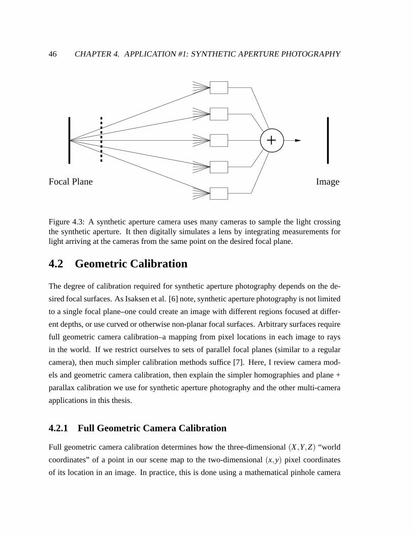
46 CHAPTER 4. APPLICATION #1: SYNTHETIC APERTURE PHOTOGRAPHY
Focal Plane
+
Image
Figure 4.3: A synthetic aperture camera uses many cameras tosample the light crossingthe synthetic aperture. It then digitally simulates a lens by integrating measurements forlight arriving at the cameras from the same point on the desired focal plane.
4.2 Geometric Calibration
The degree of calibration required for synthetic aperture photography depends on the de-
sired focal surfaces. As Isaksen et al. [6] note, synthetic aperture photography is not limited
to a single focal plane–one could create an image with different regions focused at differ-
ent depths, or use curved or otherwise non-planar focal surfaces. Arbitrary surfaces require
full geometric camera calibration–a mapping from pixel locations in each image to rays
in the world. If we restrict ourselves to sets of parallel focal planes (similar to a regular
camera), then much simpler calibration methods suffice [7].Here, I review camera mod-
els and geometric camera calibration, then explain the simpler homographies and plane +
parallax calibration we use for synthetic aperture photography and the other multi-camera
applications in this thesis.
4.2.1 Full Geometric Camera Calibration
Full geometric camera calibration determines how the three-dimensional(X ,Y,Z) “world
coordinates” of a point in our scene map to the two-dimensional (x,y) pixel coordinates
of its location in an image. In practice, this is done using a mathematical pinhole camera
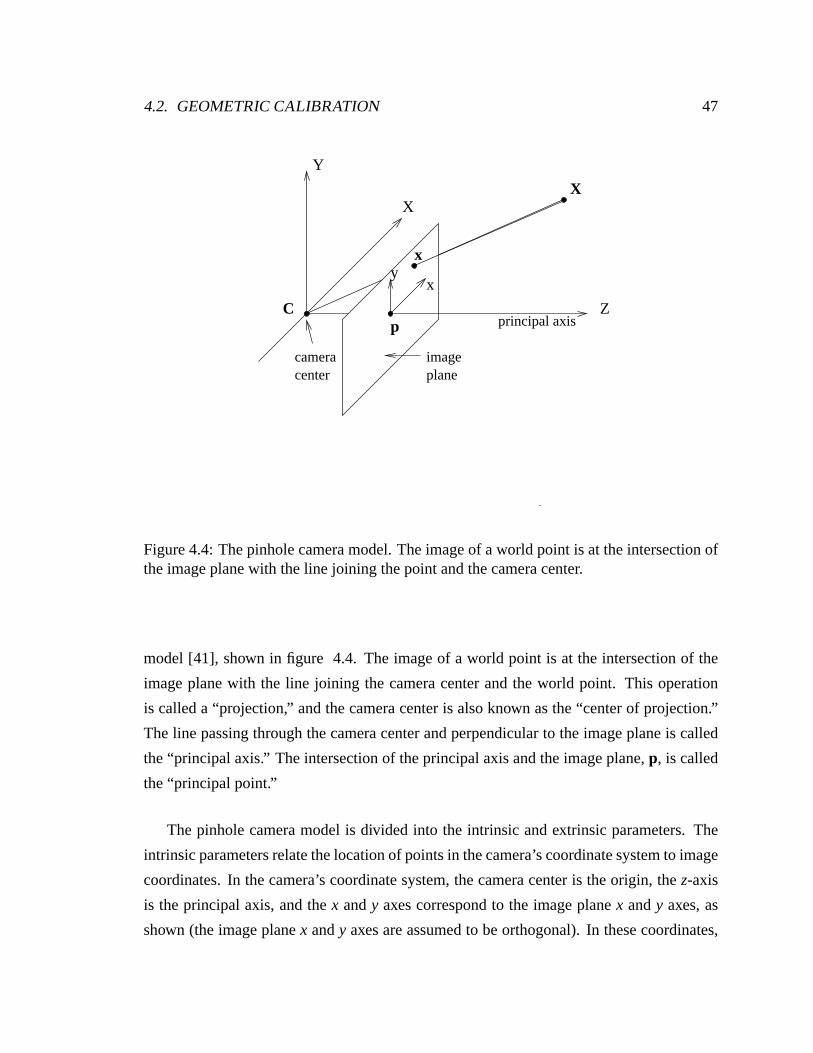
4.2. GEOMETRIC CALIBRATION 47
principal axis
imagecameracenter plane
X
Z
X
C
Y
x
xy
p
Figure 4.4: The pinhole camera model. The image of a world point is at the intersection ofthe image plane with the line joining the point and the cameracenter.
model [41], shown in figure 4.4. The image of a world point is atthe intersection of the
image plane with the line joining the camera center and the world point. This operation
is called a “projection,” and the camera center is also knownas the “center of projection.”
The line passing through the camera center and perpendicular to the image plane is called
the “principal axis.” The intersection of the principal axis and the image plane,p, is called
the “principal point.”
The pinhole camera model is divided into the intrinsic and extrinsic parameters. The
intrinsic parameters relate the location of points in the camera’s coordinate system to image
coordinates. In the camera’s coordinate system, the cameracenter is the origin, thez-axis
is the principal axis, and thex andy axes correspond to the image planex andy axes, as
shown (the image planex andy axes are assumed to be orthogonal). In these coordinates,
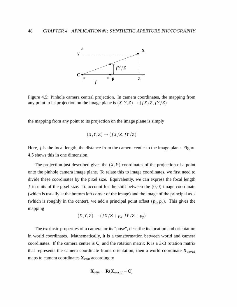
48 CHAPTER 4. APPLICATION #1: SYNTHETIC APERTURE PHOTOGRAPHY
Z
Y
Cp
fY/Z
f
X
Figure 4.5: Pinhole camera central projection. In camera coordinates, the mapping fromany point to its projection on the image plane is(X ,Y,Z) → ( f X/Z, fY/Z)
the mapping from any point to its projection on the image plane is simply
(X ,Y,Z) → ( f X/Z, fY/Z)
Here, f is the focal length, the distance from the camera center to the image plane. Figure
4.5 shows this in one dimension.
The projection just described gives the(X ,Y ) coordinates of the projection of a point
onto the pinhole camera image plane. To relate this to image coordinates, we first need to
divide these coordinates by the pixel size. Equivalently, we can express the focal length
f in units of the pixel size. To account for the shift between the (0,0) image coordinate
(which is usually at the bottom left corner of the image) and the image of the principal axis
(which is roughly in the center), we add a principal point offset(px, py). This gives the
mapping
(X ,Y,Z) → ( f X/Z + px, fY/Z + py)
The extrinsic properties of a camera, or its “pose”, describe its location and orientation
in world coordinates. Mathematically, it is a transformation between world and camera
coordinates. If the camera center isC, and the rotation matrixR is a 3x3 rotation matrix
that represents the camera coordinate frame orientation, then a world coordinateXworld
maps to camera coordinatesXcam according to
Xcam = R(Xworld −C)
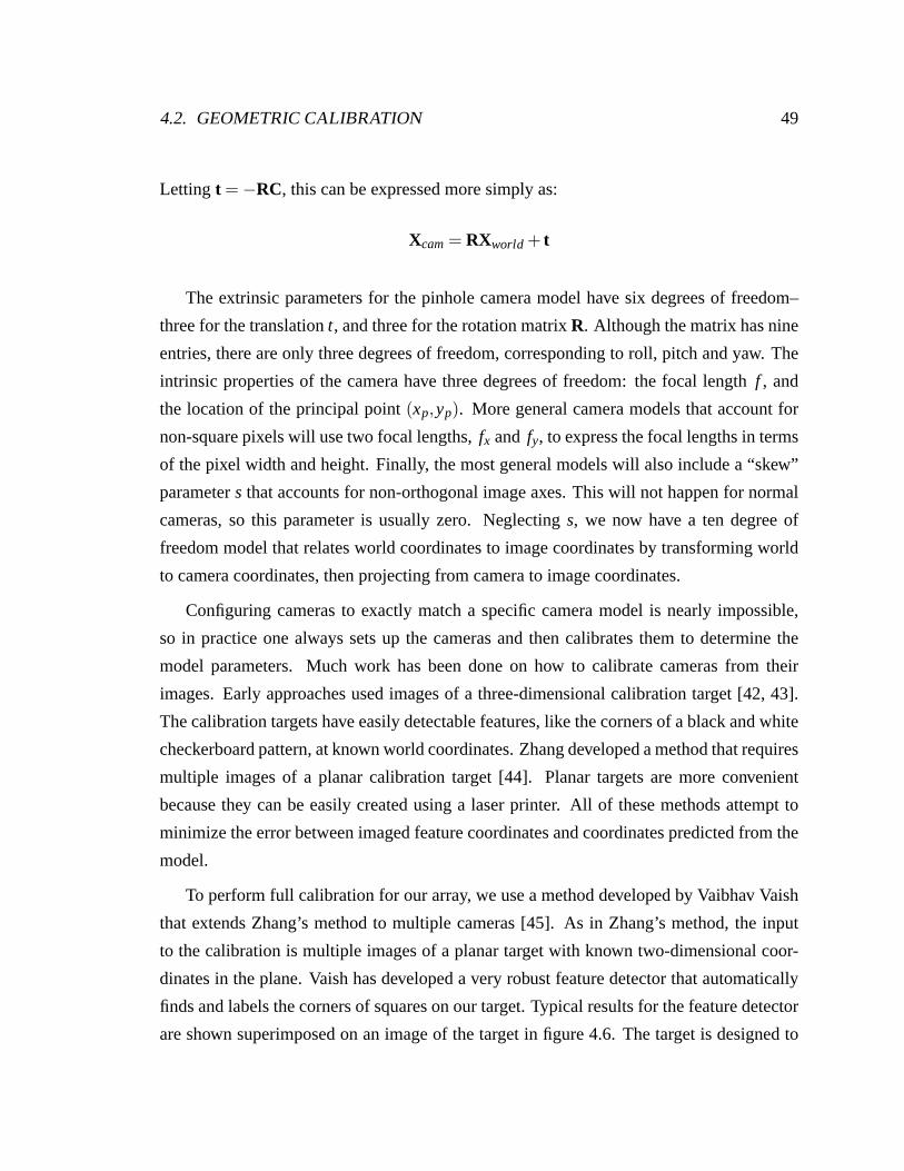
4.2. GEOMETRIC CALIBRATION 49
Letting t = −RC, this can be expressed more simply as:
Xcam = RXworld + t
The extrinsic parameters for the pinhole camera model have six degrees of freedom–
three for the translationt, and three for the rotation matrixR. Although the matrix has nine
entries, there are only three degrees of freedom, corresponding to roll, pitch and yaw. The
intrinsic properties of the camera have three degrees of freedom: the focal lengthf , and
the location of the principal point(xp,yp). More general camera models that account for
non-square pixels will use two focal lengths,fx and fy, to express the focal lengths in terms
of the pixel width and height. Finally, the most general models will also include a “skew”
parameters that accounts for non-orthogonal image axes. This will not happen for normal
cameras, so this parameter is usually zero. Neglectings, we now have a ten degree of
freedom model that relates world coordinates to image coordinates by transforming world
to camera coordinates, then projecting from camera to imagecoordinates.
Configuring cameras to exactly match a specific camera model isnearly impossible,
so in practice one always sets up the cameras and then calibrates them to determine the
model parameters. Much work has been done on how to calibratecameras from their
images. Early approaches used images of a three-dimensional calibration target [42, 43].
The calibration targets have easily detectable features, like the corners of a black and white
checkerboard pattern, at known world coordinates. Zhang developed a method that requires
multiple images of a planar calibration target [44]. Planartargets are more convenient
because they can be easily created using a laser printer. Allof these methods attempt to
minimize the error between imaged feature coordinates and coordinates predicted from the
model.
To perform full calibration for our array, we use a method developed by Vaibhav Vaish
that extends Zhang’s method to multiple cameras [45]. As in Zhang’s method, the input
to the calibration is multiple images of a planar target withknown two-dimensional coor-
dinates in the plane. Vaish has developed a very robust feature detector that automatically
finds and labels the corners of squares on our target. Typicalresults for the feature detector
are shown superimposed on an image of the target in figure 4.6.The target is designed to
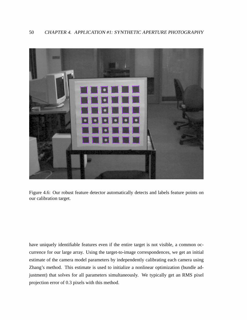
50 CHAPTER 4. APPLICATION #1: SYNTHETIC APERTURE PHOTOGRAPHY
Figure 4.6: Our robust feature detector automatically detects and labels feature points onour calibration target.
have uniquely identifiable features even if the entire target is not visible, a common oc-
currence for our large array. Using the target-to-image correspondences, we get an initial
estimate of the camera model parameters by independently calibrating each camera using
Zhang’s method. This estimate is used to initialize a nonlinear optimization (bundle ad-
justment) that solves for all parameters simultaneously. We typically get an RMS pixel
projection error of 0.3 pixels with this method.
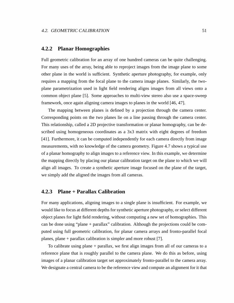
4.2. GEOMETRIC CALIBRATION 51
4.2.2 Planar Homographies
Full geometric calibration for an array of one hundred cameras can be quite challenging.
For many uses of the array, being able to reproject images from the image plane to some
other plane in the world is sufficient. Synthetic aperture photography, for example, only
requires a mapping from the focal plane to the camera image planes. Similarly, the two-
plane parametrization used in light field rendering aligns images from all views onto a
common object plane [5]. Some approaches to multi-view stereo also use a space-sweep
framework, once again aligning camera images to planes in the world [46, 47].
The mapping between planes is defined by a projection throughthe camera center.
Corresponding points on the two planes lie on a line passing through the camera center.
This relationship, called a 2D projective transformation or planar homography, can be de-
scribed using homogeneous coordinates as a 3x3 matrix with eight degrees of freedom
[41]. Furthermore, it can be computed independently for each camera directly from image
measurements, with no knowledge of the camera geometry. Figure 4.7 shows a typical use
of a planar homography to align images to a reference view. Inthis example, we determine
the mapping directly by placing our planar calibration target on the plane to which we will
align all images. To create a synthetic aperture image focused on the plane of the target,
we simply add the aligned the images from all cameras.
4.2.3 Plane + Parallax Calibration
For many applications, aligning images to a single plane is insufficient. For example, we
would like to focus at different depths for synthetic aperture photography, or select different
object planes for light field rendering, without computing anew set of homographies. This
can be done using “plane + parallax” calibration. Although the projections could be com-
puted using full geometric calibration, for planar camera arrays and fronto-parallel focal
planes, plane + parallax calibration is simpler and more robust [7].
To calibrate using plane + parallax, we first align images from all of our cameras to a
reference plane that is roughly parallel to the camera plane. We do this as before, using
images of a planar calibration target set approximately fronto-parallel to the camera array.
We designate a central camera to be the reference view and compute an alignment for it that
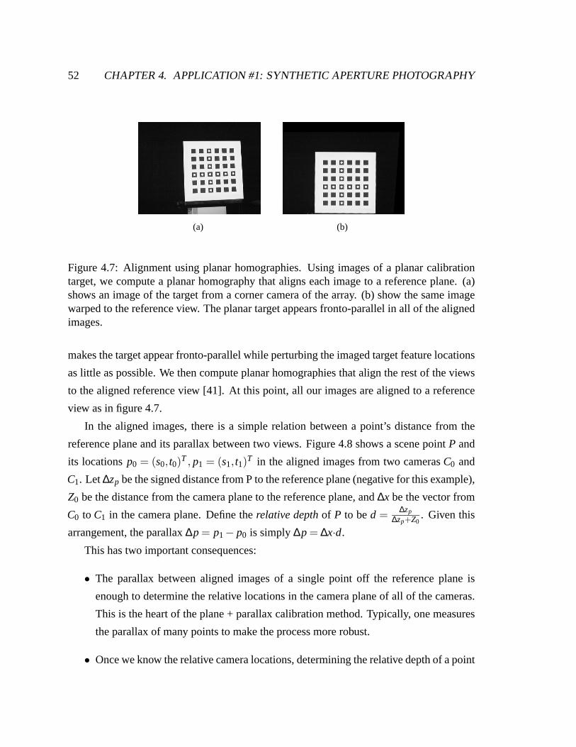
52 CHAPTER 4. APPLICATION #1: SYNTHETIC APERTURE PHOTOGRAPHY
(a) (b)
Figure 4.7: Alignment using planar homographies. Using images of a planar calibrationtarget, we compute a planar homography that aligns each image to a reference plane. (a)shows an image of the target from a corner camera of the array.(b) show the same imagewarped to the reference view. The planar target appears fronto-parallel in all of the alignedimages.
makes the target appear fronto-parallel while perturbing the imaged target feature locations
as little as possible. We then compute planar homographies that align the rest of the views
to the aligned reference view [41]. At this point, all our images are aligned to a reference
view as in figure 4.7.
In the aligned images, there is a simple relation between a point’s distance from the
reference plane and its parallax between two views. Figure 4.8 shows a scene pointP and
its locationsp0 = (s0, t0)T , p1 = (s1, t1)T in the aligned images from two camerasC0 and
C1. Let∆zp be the signed distance from P to the reference plane (negative for this example),
Z0 be the distance from the camera plane to the reference plane,and∆x be the vector from
C0 to C1 in the camera plane. Define therelative depth of P to bed =∆zp
∆zp+Z0. Given this
arrangement, the parallax∆p = p1− p0 is simply∆p = ∆x·d.
This has two important consequences:
• The parallax between aligned images of a single point off thereference plane is
enough to determine the relative locations in the camera plane of all of the cameras.
This is the heart of the plane + parallax calibration method.Typically, one measures
the parallax of many points to make the process more robust.
• Once we know the relative camera locations, determining therelative depth of a point
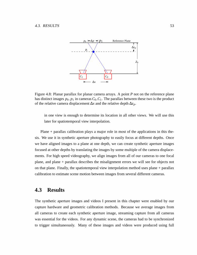
4.3. RESULTS 53
PlaneReference
Pt
∆x
p0 p1∆p
∆zp
Z0
C0C1
Figure 4.8: Planar parallax for planar camera arrays. A point P not on the reference planehas distinct imagesp0, p1 in camerasC0,C1. The parallax between these two is the productof the relative camera displacement∆x and the relative depth∆zp.
in one view is enough to determine its location in all other views. We will use this
later for spatiotemporal view interpolation.
Plane + parallax calibration plays a major role in most of theapplications in this the-
sis. We use it in synthetic aperture photography to easily focus at different depths. Once
we have aligned images to a plane at one depth, we can create synthetic aperture images
focused at other depths by translating the images by some multiple of the camera displace-
ments. For high speed videography, we align images from all of our cameras to one focal
plane, and plane + parallax describes the misalignment errors we will see for objects not
on that plane. Finally, the spatiotemporal view interpolation method uses plane + parallax
calibration to estimate scene motion between images from several different cameras.
4.3 Results
The synthetic aperture images and videos I present in this chapter were enabled by our
capture hardware and geometric calibration methods. Because we average images from
all cameras to create each synthetic aperture image, streaming capture from all cameras
was essential for the videos. For any dynamic scene, the cameras had to be synchronized
to trigger simultaneously. Many of these images and videos were produced using full
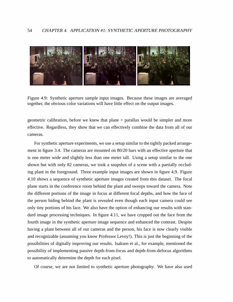
54 CHAPTER 4. APPLICATION #1: SYNTHETIC APERTURE PHOTOGRAPHY
Figure 4.9: Synthetic aperture sample input images. Becausethese images are averagedtogether, the obvious color variations will have little effect on the output images.
geometric calibration, before we knew that plane + parallaxwould be simpler and more
effective. Regardless, they show that we can effectively combine the data from all of our
cameras.
For synthetic aperture experiments, we use a setup similar to the tightly packed arrange-
ment in figure 3.4. The cameras are mounted on 80/20 bars with an effective aperture that
is one meter wide and slightly less than one meter tall. Usinga setup similar to the one
shown but with only 82 cameras, we took a snapshot of a scene with a partially occlud-
ing plant in the foreground. Three example input images are shown in figure 4.9. Figure
4.10 shows a sequence of synthetic aperture images created from this dataset. The focal
plane starts in the conference room behind the plant and sweeps toward the camera. Note
the different portions of the image in focus at different focal depths, and how the face of
the person hiding behind the plant is revealed even though each input camera could see
only tiny portions of his face. We also have the option of enhancing our results with stan-
dard image processing techniques. In figure 4.11, we have cropped out the face from the
fourth image in the synthetic aperture image sequence and enhanced the contrast. Despite
having a plant between all of our cameras and the person, his face is now clearly visible
and recognizable (assuming you know Professor Levoy!). This is just the beginning of the
possibilities of digitally improving our results. Isaksenet al., for example, mentioned the
possibility of implementing passive depth-from-focus anddepth-from-defocus algorithms
to automatically determine the depth for each pixel.
Of course, we are not limited to synthetic aperture photography. We have also used
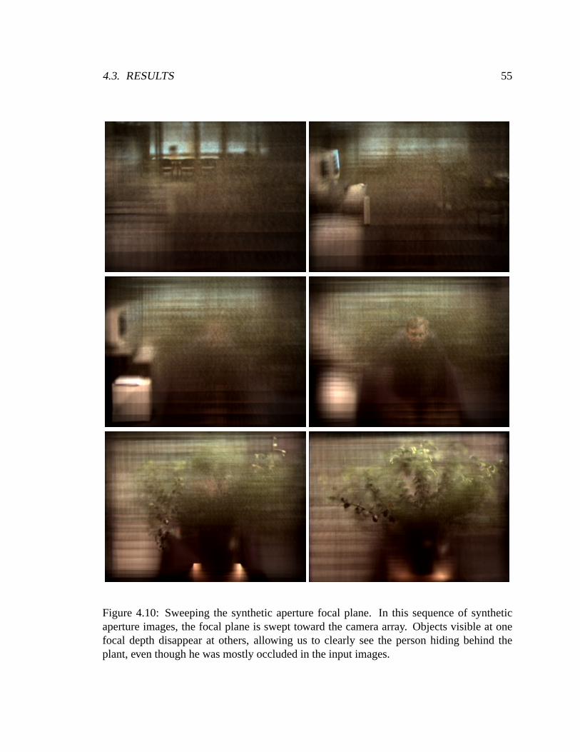
4.3. RESULTS 55
Figure 4.10: Sweeping the synthetic aperture focal plane. In this sequence of syntheticaperture images, the focal plane is swept toward the camera array. Objects visible at onefocal depth disappear at others, allowing us to clearly see the person hiding behind theplant, even though he was mostly occluded in the input images.

56 CHAPTER 4. APPLICATION #1: SYNTHETIC APERTURE PHOTOGRAPHY
Figure 4.11: A synthetic aperture image with enhanced contrast.
Figure 4.12: Synthetic aperture video sample input images.
the array to create the world’s first synthetic aperture videos of dynamic scenes. Using the
same setup as before, we streamed synchronized, 4Mb/s MPEG video from all cameras to
disk. The scene is three people walking behind a dense wall ofvines. Three sample images
from different cameras at the same time (with a person behindthe vines) are shown in
figure 4.12. These images actually make the situation seem worse than it really is. Viewing
any one input video, one can tell that people are moving behind the vines, although it is
not possible to tell who they are or what they are doing. I haveincluded an example input
video, sapvideoinput.mpg, on the CD-ROM accompanying this thesis.
The resulting synthetic aperture video is also on the CD-ROM,labeled sapvideo.mpg.
In it, we see the three people moving behind the wall of vines and some of the objects they
are carrying. Example frames are shown in figure 4.13.
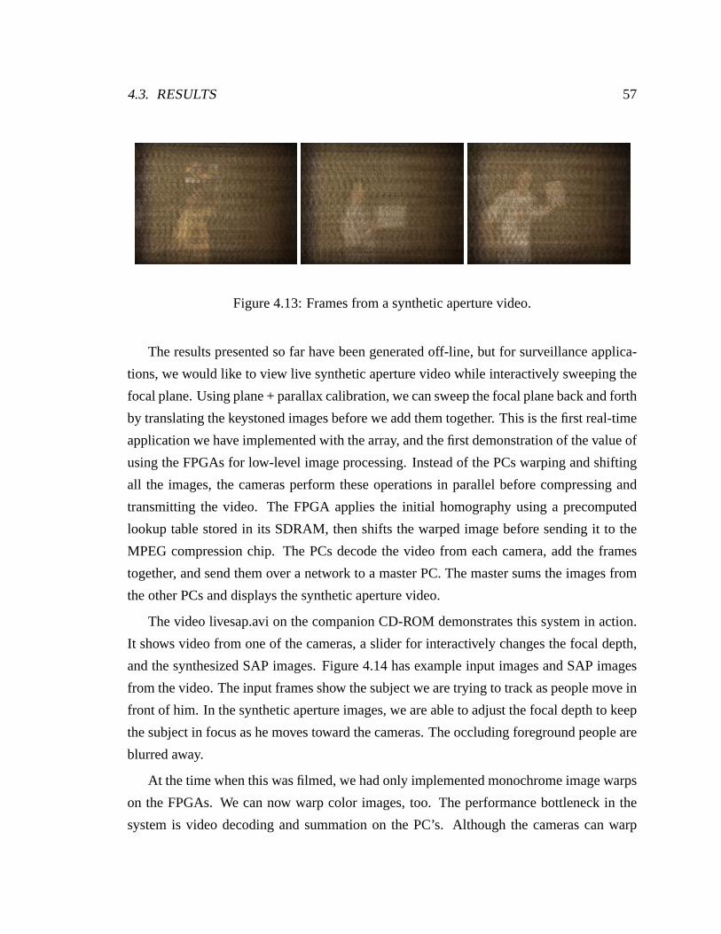
4.3. RESULTS 57
Figure 4.13: Frames from a synthetic aperture video.
The results presented so far have been generated off-line, but for surveillance applica-
tions, we would like to view live synthetic aperture video while interactively sweeping the
focal plane. Using plane + parallax calibration, we can sweep the focal plane back and forth
by translating the keystoned images before we add them together. This is the first real-time
application we have implemented with the array, and the firstdemonstration of the value of
using the FPGAs for low-level image processing. Instead of the PCs warping and shifting
all the images, the cameras perform these operations in parallel before compressing and
transmitting the video. The FPGA applies the initial homography using a precomputed
lookup table stored in its SDRAM, then shifts the warped imagebefore sending it to the
MPEG compression chip. The PCs decode the video from each camera, add the frames
together, and send them over a network to a master PC. The master sums the images from
the other PCs and displays the synthetic aperture video.
The video livesap.avi on the companion CD-ROM demonstrates this system in action.
It shows video from one of the cameras, a slider for interactively changes the focal depth,
and the synthesized SAP images. Figure 4.14 has example input images and SAP images
from the video. The input frames show the subject we are trying to track as people move in
front of him. In the synthetic aperture images, we are able toadjust the focal depth to keep
the subject in focus as he moves toward the cameras. The occluding foreground people are
blurred away.
At the time when this was filmed, we had only implemented monochrome image warps
on the FPGAs. We can now warp color images, too. The performance bottleneck in the
system is video decoding and summation on the PC’s. Although the cameras can warp
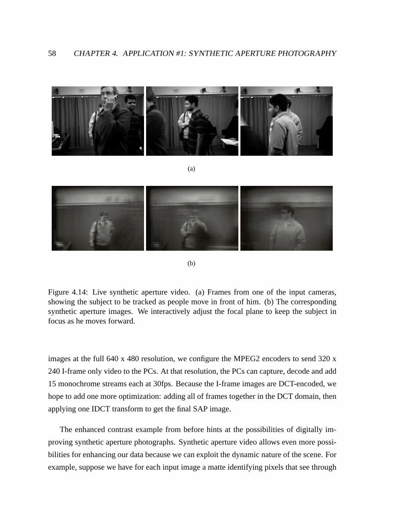
58 CHAPTER 4. APPLICATION #1: SYNTHETIC APERTURE PHOTOGRAPHY
(a)
(b)
Figure 4.14: Live synthetic aperture video. (a) Frames fromone of the input cameras,showing the subject to be tracked as people move in front of him. (b) The correspondingsynthetic aperture images. We interactively adjust the focal plane to keep the subject infocus as he moves forward.
images at the full 640 x 480 resolution, we configure the MPEG2encoders to send 320 x
240 I-frame only video to the PCs. At that resolution, the PCs can capture, decode and add
15 monochrome streams each at 30fps. Because the I-frame images are DCT-encoded, we
hope to add one more optimization: adding all of frames together in the DCT domain, then
applying one IDCT transform to get the final SAP image.
The enhanced contrast example from before hints at the possibilities of digitally im-
proving synthetic aperture photographs. Synthetic aperture video allows even more possi-
bilities for enhancing our data because we can exploit the dynamic nature of the scene. For
example, suppose we have for each input image a matte identifying pixels that see through

4.3. RESULTS 59
(a) (b)
Figure 4.15: Synthetic aperture with occluder mattes. (a) Aregular synthetic apertureimage, averaged from all aligned input images. (b) Each pixel in this image is the averageof only the corresponding input image pixels that see through the occluder. The contrast isgreatly increased because the occluder is eliminated instead of blurred.
the foreground occluder. If instead of averaging pixels from all images to generate the syn-
thetic aperture image, we average only those that see the background, we can eliminate the
occluder instead of blurring it away. For a static occluder,there are many ways to generate
these mattes. For example, we could place a black surface behind the object, then a white
one, and record which pixels change.
Figure 4.15 shows an experiment using another approach—masking all of the pixels
which never change during the recorded video. These pixels correspond to the static parts
of the video, either the background or the occluder. In practice, we use a threshold so we
do not confuse image noise with unoccluded pixels. The imageon the left is the usual
synthetic aperture image. On the right, each pixel is the average of only the unoccluded
pixels in the input images, and the image contrast is much improved. The missing pixels
are ones in which no camera saw through the foreground, nothing changed during the video
segment, or the changes were below our threshold.
Pixels that contain a mixture of foreground and background colors will corrupt the mat-
ted results, and we can expect that our Bayer demosaicing willwork poorly for background

60 CHAPTER 4. APPLICATION #1: SYNTHETIC APERTURE PHOTOGRAPHY
colors unless the holes in the occluder are several pixels wide. Color calibration also be-
comes an issue here. Regular synthetic aperture photographyis relatively insensitive to
the varying color responses of our sensors. The cameras usedto take the images in fig-
ure 4.9 were configured identically, but show significant variation. Because the data from
all the cameras are averaged together, the differences are averaged away. For the matting
experiment, if few values are averaged for a pixel, color variations will have a greater ef-
fect. In the next section, we will look at an application witheven stricter color calibration
requirements: high-speed video capture using a dense camera array.
Chapter 5
Application #2: High-Speed
Videography
This chapter explains how we use our camera array as a high-speed video camera by stag-
gering the shutter times of the cameras and interleaving their aligned and color-corrected
images. Creating a single high-speed camera from the array requires a combination of fine
control over the cameras and compensation for varying geometric and radiometric prop-
erties characteristic of cheap image sensors. Interleaving images from different cameras
means that uncorrected variations in their radiometric properties will cause frame-to-frame
intensity and color differences in the high-speed video. Because the radiometric responses
of cheap cameras varies greatly, the cameras in our array must be configured to have rel-
atively similar responses, then calibrated so the remaining differences can be corrected in
post-processing.
High-speed videography stresses the temporal accuracy of every imaged pixel, so we
must correct for distortions of fast-moving objects due to the electronic rolling shutter in
our CMOS image sensors. Rolling shutter images can be thought of as diagonal planes in
a spatiotemporal volume, and slicing the volume of rolling shutter images along vertical
planes of constant time eliminates the distortions. At the end of the chaptor, I will explore
ways to extend performance by taking advantage of the uniquefeatures of multiple camera
sensors—parallel compression for very long recordings, and exposure windows that span
multiple high-speed frame times for increasing the frame rate or signal-to-noise ratio. The
61
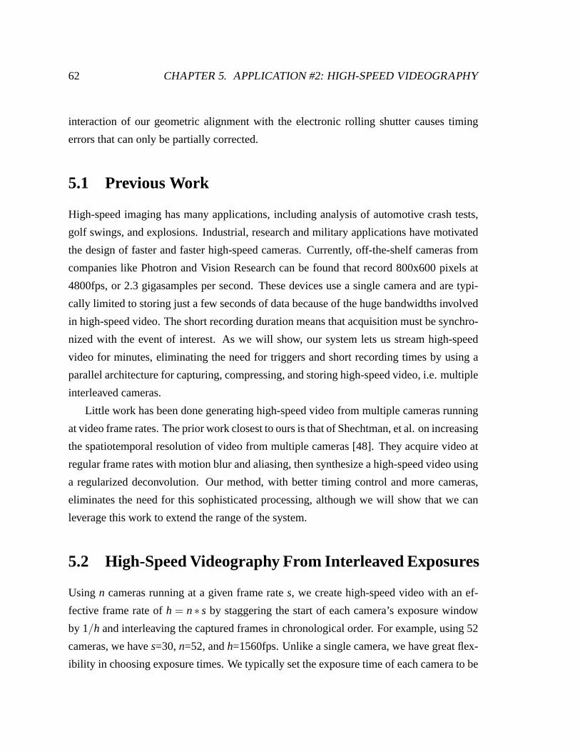
62 CHAPTER 5. APPLICATION #2: HIGH-SPEED VIDEOGRAPHY
interaction of our geometric alignment with the electronicrolling shutter causes timing
errors that can only be partially corrected.
5.1 Previous Work
High-speed imaging has many applications, including analysis of automotive crash tests,
golf swings, and explosions. Industrial, research and military applications have motivated
the design of faster and faster high-speed cameras. Currently, off-the-shelf cameras from
companies like Photron and Vision Research can be found that record 800x600 pixels at
4800fps, or 2.3 gigasamples per second. These devices use a single camera and are typi-
cally limited to storing just a few seconds of data because ofthe huge bandwidths involved
in high-speed video. The short recording duration means that acquisition must be synchro-
nized with the event of interest. As we will show, our system lets us stream high-speed
video for minutes, eliminating the need for triggers and short recording times by using a
parallel architecture for capturing, compressing, and storing high-speed video, i.e. multiple
interleaved cameras.
Little work has been done generating high-speed video from multiple cameras running
at video frame rates. The prior work closest to ours is that ofShechtman, et al. on increasing
the spatiotemporal resolution of video from multiple cameras [48]. They acquire video at
regular frame rates with motion blur and aliasing, then synthesize a high-speed video using
a regularized deconvolution. Our method, with better timing control and more cameras,
eliminates the need for this sophisticated processing, although we will show that we can
leverage this work to extend the range of the system.
5.2 High-Speed Videography From Interleaved Exposures
Using n cameras running at a given frame rates, we create high-speed video with an ef-
fective frame rate ofh = n ∗ s by staggering the start of each camera’s exposure window
by 1/h and interleaving the captured frames in chronological order. For example, using 52
cameras, we haves=30,n=52, andh=1560fps. Unlike a single camera, we have great flex-
ibility in choosing exposure times. We typically set the exposure time of each camera to be

5.2. HIGH-SPEED VIDEOGRAPHY FROM INTERLEAVED EXPOSURES 63
Figure 5.1: An array of 52 cameras for capturing high-speed video. The cameras are packedclosely together to approximate a single center of projection.
1/h, 650µs in this case, or less. The exposure duration for our Omnivision sensors is pro-
grammable in increments of 205µs, corresponding to four row times. Very short exposure
times are often light-limited, creating a trade-off between acquiring more light (to improve
the signal-to-noise ratio) using longer exposures, and reducing motion blur with shorter
exposures. Because we use multiple cameras, we have the option of extending our expo-
sure times past 1/h to gather more light and using temporal super-resolution techniques to
compute high-speed video. We will return to these ideas later.
Figure 5.1 shows the assembly of 52 cameras used for these experiments. To align
images from the different cameras to a single reference view, we make the simplifying as-
sumption that the scene lies within a shallow depth of a single object plane. Under these
conditions, we can register images using planar homographies as described in section 4.2.
We place the calibration target at the assumed object plane and pick one of the central
cameras in the array to be the reference view. Using automatically detected feature corre-
spondences between images, we compute alignment homographies for all other views to
the reference view.
Of course, this shallow scene assumption holds only for scenes that are relatively flat
or sufficiently distant from the array relative to the cameraspacing. Figure 5.2 shows the
alignment error as objects stray from the object plane. In this analysis, (although not in our
calibration procedure), we assume that our cameras are located on a plane, their optical axes
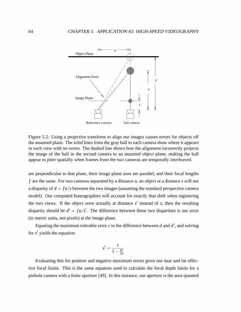
64 CHAPTER 5. APPLICATION #2: HIGH-SPEED VIDEOGRAPHY
s
s’
f
Alignment Error
Object Plane
Image Plane
2nd camera
a
Reference camera
Figure 5.2: Using a projective transform to align our imagescauses errors for objects offthe assumed plane. The solid lines from the gray ball to each camera show where it appearsin each view with no errors. The dashed line shows how the alignment incorrectly projectsthe image of the ball in the second camera to an assumed objectplane, making the ballappear to jitter spatially when frames from the two cameras are temporally interleaved.
are perpendicular to that plane, their image plane axes are parallel, and their focal lengths
f are the same. For two cameras separated by a distancea, an object at a distances will see
a disparity ofd = f a/s between the two images (assuming the standard perspective camera
model). Our computed homographies will account for exactlythat shift when registering
the two views. If the object were actually at distances′ instead ofs, then the resulting
disparity should bed′ = f a/s′. The difference between these two disparities is our error
(in metric units, not pixels) at the image plane.
Equating the maximum tolerable errorc to the difference betweend andd′, and solving
for s′ yields the equation
s′ =s
1− scf a
Evaluating this for positive and negative maximum errors gives our near and far effec-
tive focal limits. This is the same equation used to calculate the focal depth limits for a
pinhole camera with a finite aperture [49]. In this instance,our aperture is the area spanned

5.2. HIGH-SPEED VIDEOGRAPHY FROM INTERLEAVED EXPOSURES 65
Focal Length Focal Distance Depth of Field Hyperfocal Distance
10m 0.82m6.0mm 20m 3.3m 242m
30m 7.5m100m 99m10m 0.24m
20.0mm 20m 0.99m 809m30m 2.2m
100m 25m
Table 5.1: The effective depth of field for the 52-camera array for different lens focallengths and object focal distances.
by our camera locations. Rather than becoming blurry, objects off the focal plane remain
sharp but appear to move around from frame to frame in the aligned images.
For our lab setup, the object plane is 3m from our cameras, thecamera pitch is 33mm,
and the maximum separation between any two of the 52 cameras is 251mm. The image
sensors have a 6mm focal length and a pixel size of 6.2µm. Choosing a maximum toler-
able error of +/- one pixel, we get near and far focal depth limits of 2.963m and 3.036m,
respectively, for a total depth of field of 7.3cm.
Note that these numbers are a consequence of filming in a confined laboratory. For
many high-speed video applications, the objects of interest are sufficiently far away to
allow much higher effective depths of field. To give an idea ofhow our system would
work in such settings, table 5.1 shows how the depth of field grows with object focal depth.
It presents two arrangements, the lab setup with 6mm lenses already described, and the
same rig with moderately telephoto 20mm lenses. The depth offield grows quickly with
distance. For the system with 6mm lenses and an object focal distance of 10m, the depth
of field is already nearly a meter. The table also includes theeffective hyperfocal distance,
h, for the systems. When the object focal depth is set ath, the effective depth of field of the
system becomes infinite. The motion in the aligned images of all objects farther thanh/2
from the camera array will be less than our maximum tolerableerror.
The false motion of off-plane objects can be rendered much less visually objectionable
by ensuring that sequential cameras in time are spatially adjacent in the camera mount. This
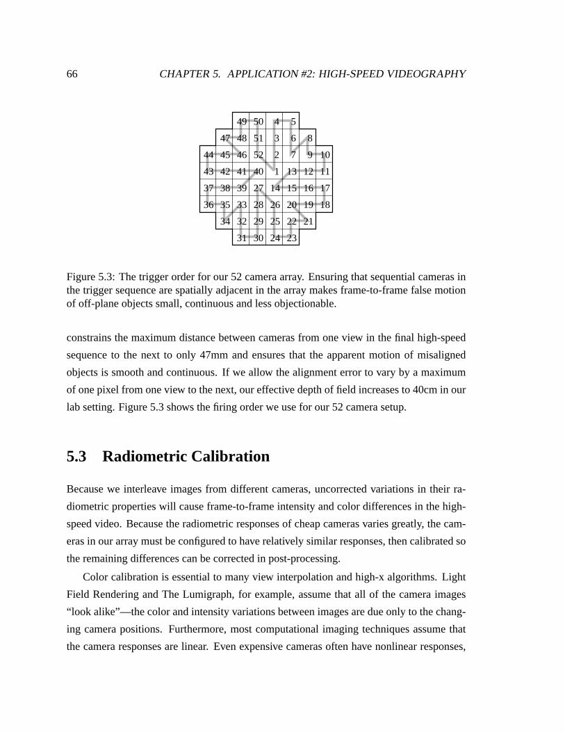
66 CHAPTER 5. APPLICATION #2: HIGH-SPEED VIDEOGRAPHY
1
2
3
4 5
86
7 9 10
111213
14 15 16 17
181920
2122
2324
25
26
27
28
29
3031
32
33
34
3536
37 38 39
40414243
44 45 46
47 48
49 50
51
52
Figure 5.3: The trigger order for our 52 camera array. Ensuring that sequential cameras inthe trigger sequence are spatially adjacent in the array makes frame-to-frame false motionof off-plane objects small, continuous and less objectionable.
constrains the maximum distance between cameras from one view in the final high-speed
sequence to the next to only 47mm and ensures that the apparent motion of misaligned
objects is smooth and continuous. If we allow the alignment error to vary by a maximum
of one pixel from one view to the next, our effective depth of field increases to 40cm in our
lab setting. Figure 5.3 shows the firing order we use for our 52camera setup.
5.3 Radiometric Calibration
Because we interleave images from different cameras, uncorrected variations in their ra-
diometric properties will cause frame-to-frame intensityand color differences in the high-
speed video. Because the radiometric responses of cheap cameras varies greatly, the cam-
eras in our array must be configured to have relatively similar responses, then calibrated so
the remaining differences can be corrected in post-processing.
Color calibration is essential to many view interpolation and high-x algorithms. Light
Field Rendering and The Lumigraph, for example, assume that all of the camera images
“look alike”—the color and intensity variations between images are due only to the chang-
ing camera positions. Furthermore, most computational imaging techniques assume that
the camera responses are linear. Even expensive cameras often have nonlinear responses,
5.3. RADIOMETRIC CALIBRATION 67
so we must also find a way to linearize the sensor response. Fora large camera array, these
calibration methods must be automatic.
Differences in the response of a camera’s pixels to incidentillumination from the scene
can be due to variations in the sensor’s response or to the camera’s optics. Here, I summa-
rize these sources of variation, review past efforts to automatically radiometrically calibrate
camera arrays, and present methods for automatically configuring and color matching the
array.
5.3.1 Camera Radiometric Variations
For a given incident illumination, a camera’s image sensor and optics determine its radio-
metric response. Process variations between sensors (or even between pixels on the same
sensor) lead to different responses at each step of the imaging process. The color filters for
single-chip color sensors, the photodetectors that collect stray electrons generated by light
interacting with silicon, and the circuitry for amplifyingand reading out the values sensed
at each pixel all contribute to the variations between sensors. The CMOS sensors in our
array use “analog processing” for color space conversion and gamma adjustment, adding
more sources of variation unless these features are turned off.
The optics on our cameras also cause variations in color response. Cos4 falloff and
vignetting, for example, cause images to get dimmer towardsthe edges. Less strict man-
ufacturing tolerances for inexpensive lenses also lead to differences in the amount of light
they gather. Global differences in the amount of light a lenspasses to the sensor are in-
distinguishable from a global change in the gain of the sensor, so we do not attempt to
calibrate our sensor and lenses separately. Furthermore, although intensity falloff is cer-
tainly significant for our cameras, we have not yet attemptedto calibrate it for our array.
Our experience so far has been that it is roughly similar fromcamera to camera and does
not strongly impact our algorithms.
5.3.2 Prior Work in Color Calibrating Large Camera Arrays
Very little work has been done on automatically radiometrically calibrating large camera
arrays, most likely because big arrays are still rare. Some systems, such as the 3D-Room,
68 CHAPTER 5. APPLICATION #2: HIGH-SPEED VIDEOGRAPHY
do not color calibrate their cameras at all, leading to colorartifacts [50]. Presumably the
automatic gain, offset and white balance controls for theircameras produced acceptable
images, even if they varied somewhat between cameras. Yang et al. found that the au-
tomatic controls were unreliable for their 64-camera array[15], so they used the method
proposed by Nanda and Cutler for an omnidirectional multi-sensor “RingCam” [51].
The RingCam itself was a set of cameras with only partially overlapping views, so the
color calibration relies on image statistics in the region of overlap between neighboring
cameras. Because this method is the only other one we know of for configuring an array
of cameras, I will briefly describe it here before presentingour methods. In the notation of
Nanda and Cutler, for a camera with brightnessb and contrastc, the relation between an
observed pixel valueI(x,y) and the accumulated chargei(x,y) on the sensor at that pixel is
I(x,y) = b+ c∗ i(x,y)
Their image sensors, like ours, have programmable gains (contrasts) and offsets (bi-
ases). To configure their cameras, they first set the contrastfor their sensors to zero and
adjust the offset until the mean image value is some designated “black value.” Once the
offset has been fixed, they vary the contrast to raise the meanimage value to some user-
selected level. Finally, they white balance their cameras by filming a white piece of paper
and adjusting the red and blue gains of their sensors until the images of the paper have
equal red, green and blue components. Their goal was real-time image corrections, so they
did not implement any post-processing of the images from their cameras.
Our color calibration goals are different from those of Nanda et al. The RingCam had
to deal with highly varying illumination because their cameras had only partially overlap-
ping fields of view and were arranged to cumulatively span a full 360 degrees. For the
applications in this thesis, our cameras are usually on a plane and verged to view a com-
mon working volume, so the ranges of intensities in the viewsare more consistent. The
RingCam was designed to handle dynamically varying illumination and used blending to
mitigate residual color differences between cameras. Our goal is to produce images that
require no blending. We fix our camera settings at the start ofeach acquisition so we can
calibrate for a particular setting and post-process the images to correct for variations.
5.3. RADIOMETRIC CALIBRATION 69
5.3.3 Radiometric Calibration Method
Our calibration method ensures that all cameras view the same range of scene intensities
and maximizes the usable data produced in each color channelby all cameras so we can
process it later. It is described in detail in Neel Joshi’s Master’s thesis [8]. We start by con-
figuring all of our cameras to match the same desired linear fitfor the gray scale checkers
on a Macbeth color checker chart. Our image sensors are highly nonlinear near the top and
bottom of their output range, so we fit the response to a line from 20 (out of 255) for the
black patch (3.1% reflectance) to 220 for the white patch (90.0% reflectance). We itera-
tively adjust the programmable green, red and blue gains andoffsets on our sensors until
the measured responses match the line. Assuming the white patch is the brightest object in
our scene, this ensures that we’re using the entire range of each color channel and reduces
quantization noise in our images. This linear fit has the added benefit of white balancing
our cameras.
To ensure that intensity falloff and uneven illumination donot cause errors, we take an
image with a photographic gray card in place of the checker chart. With no intensity falloff
and uniform illumination, the image of this diffuse gray card would be constant at all pixels.
For each camera, we compute scale values for each pixel that correct the nonuniformity and
apply them to all image measurements.
Once we have automatically configured the cameras, we apply standard methods to
further improve the color uniformity of images. The image sensor response is only roughly
linear, so we compute lookup tables to map the slightly nonlinear responses of our cameras
to the desired line for the gray scale patches. Then we compute 3x3 correction matrices
that we apply to the(R,G,B) pixel values from each camera to generate corrected(R,G,B)
values. The matrices minimize the variance between measured values for all of the color
checkers in the chart across all of the cameras in the array.
There are a number of ways one could automate this task. We chose to leverage our
geometric calibration by attaching the color checker to outgeometric calibration target at
a fixed location and using homographies to automatically findthe locations of the color
checker patches. With this method, we can robustly and simply radiometrically configure
and calibrate an array of 100 cameras in a matter of minutes.

70 CHAPTER 5. APPLICATION #2: HIGH-SPEED VIDEOGRAPHY
Figure 5.4: A color checker mosaic with no color correction.This image was assembled us-ing 7x7 blocks from different cameras and clearly shows the radiometric variation betweenthem, even though they are configured with identical exposure and color gain settings.
Figure 5.4 shows an image mosaic of a Macbeth color checker chart made with no color
calibration. To make this image, we configured all of our cameras with the same gains, took
pictures of the target and then applied the planar homography described earlier to warp all
the images to one common reference view. We assembled the mosaic from 7x7 pixel blocks
from different camera images. Each diagonal line of blocks (diagonal from lower left to
upper right) is from the same camera. The color differences are easy to see in this image
and give an idea of the process variation between image sensors.
In the figure 5.5 below, we have used our color calibration routines to properly set up
the cameras and post-process the images. Note that the colordifferences are very hard
to detect visually. This implies that we should be able to do other types of mosaics and
IBR methods for combining images effectively, too. In quantitative terms, the RMS error
between color values for any two cameras was 1.7 for red values, 1.0 for green, and 1.4 for
blue. The maximum error was larger, 11 for red, 6 for green and8 for blue. Although the
perceptible differences in the resulting images are small,the large maximum errors might
cause difficulties for vision algorithms that rely on accurate color information. As we will
see in the next chapter, we have successfully use optical flowbased vision algorithms on
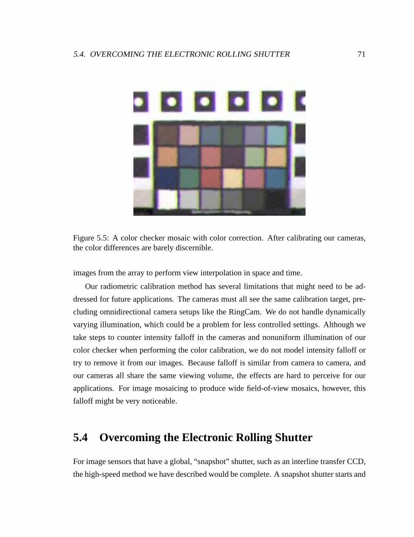
5.4. OVERCOMING THE ELECTRONIC ROLLING SHUTTER 71
Figure 5.5: A color checker mosaic with color correction. After calibrating our cameras,the color differences are barely discernible.
images from the array to perform view interpolation in spaceand time.
Our radiometric calibration method has several limitations that might need to be ad-
dressed for future applications. The cameras must all see the same calibration target, pre-
cluding omnidirectional camera setups like the RingCam. We donot handle dynamically
varying illumination, which could be a problem for less controlled settings. Although we
take steps to counter intensity falloff in the cameras and nonuniform illumination of our
color checker when performing the color calibration, we do not model intensity falloff or
try to remove it from our images. Because falloff is similar from camera to camera, and
our cameras all share the same viewing volume, the effects are hard to perceive for our
applications. For image mosaicing to produce wide field-of-view mosaics, however, this
falloff might be very noticeable.
5.4 Overcoming the Electronic Rolling Shutter
For image sensors that have a global, “snapshot” shutter, such as an interline transfer CCD,
the high-speed method we have described would be complete. Asnapshot shutter starts and
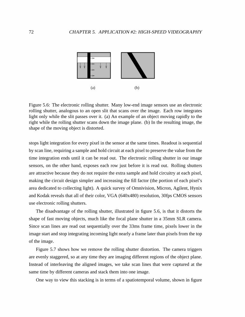
72 CHAPTER 5. APPLICATION #2: HIGH-SPEED VIDEOGRAPHY
(a) (b)
Figure 5.6: The electronic rolling shutter. Many low-end image sensors use an electronicrolling shutter, analogous to an open slit that scans over the image. Each row integrateslight only while the slit passes over it. (a) An example of an object moving rapidly to theright while the rolling shutter scans down the image plane. (b) In the resulting image, theshape of the moving object is distorted.
stops light integration for every pixel in the sensor at the same times. Readout is sequential
by scan line, requiring a sample and hold circuit at each pixel to preserve the value from the
time integration ends until it can be read out. The electronic rolling shutter in our image
sensors, on the other hand, exposes each row just before it isread out. Rolling shutters
are attractive because they do not require the extra sample and hold circuitry at each pixel,
making the circuit design simpler and increasing the fill factor (the portion of each pixel’s
area dedicated to collecting light). A quick survey of Omnivision, Micron, Agilent, Hynix
and Kodak reveals that all of their color, VGA (640x480) resolution, 30fps CMOS sensors
use electronic rolling shutters.
The disadvantage of the rolling shutter, illustrated in figure 5.6, is that it distorts the
shape of fast moving objects, much like the focal plane shutter in a 35mm SLR camera.
Since scan lines are read out sequentially over the 33ms frame time, pixels lower in the
image start and stop integrating incoming light nearly a frame later than pixels from the top
of the image.
Figure 5.7 shows how we remove the rolling shutter distortion. The camera triggers
are evenly staggered, so at any time they are imaging different regions of the object plane.
Instead of interleaving the aligned images, we take scan lines that were captured at the
same time by different cameras and stack them into one image.
One way to view this stacking is in terms of a spatiotemporal volume, shown in figure

5.4. OVERCOMING THE ELECTRONIC ROLLING SHUTTER 73
� � �� � �� � �� � �� � �� � �
� �� �� �� �� �� �
� � �� � �� � �� � �� � �� � �
� � �� � �� � �� � �� � �� � �
� �� �� �� �� �� �
� �� �� �� �� �� �
� � �� � �� � �� � �� � �� � �
� �� �� �� �� �� �
� � �� � �� � �� � �� � �� � �
� �� �� �� �� �� �
Figure 5.7: Correcting the electronic rolling shutter distortion. The images on the leftrepresent views from five cameras with staggered shutters. At any time, different rows(shown in gray) in each camera are imaging the object plane. Bystacking these rows intoone image, we create a view with no distortion.
y
tx
(a)
y
tx
(b)
Figure 5.8: Slicing the spatiotemporal volume to correct rolling shutter distortion. (a)Cameras with global shutters capture their entire image at the same time, so each one isa vertical slice in the volume. (b) Cameras with rolling shutters capture lower rows intheir images later in time, so each frame lies on a slanted plane in the volume. Slicingrolling shutter video along planes of constant time in the spatiotemporal volume removesthe distortion.
5.8. Images from cameras with global shutters are vertical slices (along planes of constant
time) of the spatiotemporal volume. Images from rolling shutter cameras, on the other
hand, are diagonal slices in the spatiotemporal volume. Thescan line stacking we just de-
scribed is equivalent to slicing the volume of rolling shutter images along planes of constant
time. We use trilinear interpolation between frames to create the images. The slicing re-
sults in smooth, undistorted images. Figure 5.9 shows a comparison of frames from sliced
and unsliced videos of a rotating fan. The videos were filmed with the 52 camera setup,
using the trigger ordering in figure 5.3.
The spatiotemporal analysis so far neglects the interaction between the rolling shutter
and our image alignments. Vertical components in the alignment transformations raise or
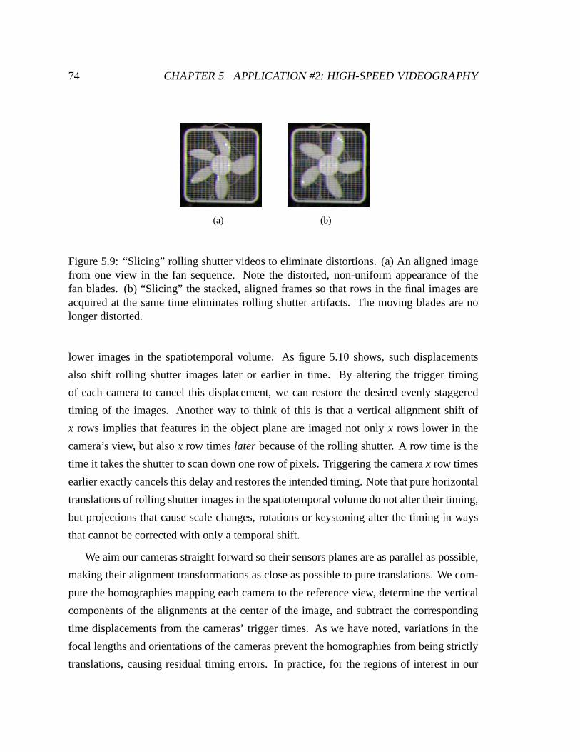
74 CHAPTER 5. APPLICATION #2: HIGH-SPEED VIDEOGRAPHY
(a) (b)
Figure 5.9: “Slicing” rolling shutter videos to eliminate distortions. (a) An aligned imagefrom one view in the fan sequence. Note the distorted, non-uniform appearance of thefan blades. (b) “Slicing” the stacked, aligned frames so that rows in the final images areacquired at the same time eliminates rolling shutter artifacts. The moving blades are nolonger distorted.
lower images in the spatiotemporal volume. As figure 5.10 shows, such displacements
also shift rolling shutter images later or earlier in time. Byaltering the trigger timing
of each camera to cancel this displacement, we can restore the desired evenly staggered
timing of the images. Another way to think of this is that a vertical alignment shift of
x rows implies that features in the object plane are imaged notonly x rows lower in the
camera’s view, but alsox row timeslater because of the rolling shutter. A row time is the
time it takes the shutter to scan down one row of pixels. Triggering the camerax row times
earlier exactly cancels this delay and restores the intended timing. Note that pure horizontal
translations of rolling shutter images in the spatiotemporal volume do not alter their timing,
but projections that cause scale changes, rotations or keystoning alter the timing in ways
that cannot be corrected with only a temporal shift.
We aim our cameras straight forward so their sensors planes are as parallel as possible,
making their alignment transformations as close as possible to pure translations. We com-
pute the homographies mapping each camera to the reference view, determine the vertical
components of the alignments at the center of the image, and subtract the corresponding
time displacements from the cameras’ trigger times. As we have noted, variations in the
focal lengths and orientations of the cameras prevent the homographies from being strictly
translations, causing residual timing errors. In practice, for the regions of interest in our

5.5. RESULTS 75
y
tx
(a)
y
tx
(b)
Figure 5.10: Alignment of rolling shutter images in the spatiotemporal volume. (a) Verti-cally translating rolling shutter images displaces them toward planes occupied by earlier orlater frames. This is effectively a temporal offset in the image. (b) Translating the imagein time by altering the camera shutter timing corrects the offset. As a result, the image istranslated along its original spatiotemporal plane.
videos (usually the center third of the images) the maximum error is typically under two
row times. At 1560fps, the frames are twelve row times apart.
The timing offset error by the rolling shutter is much easierto see in a video than in a se-
quence of still frames. The video faneven.mpg on the CD-ROM accompanying this thesis
shows a fan filmed at 1560fps using our 52 camera setup and evenly staggered trigger times.
The fan appears to speed up and slow down, although its real velocity is constant. Note
that the effect of the timing offsets is lessened by our sampling order—neighboring cameras
have similar alignment transformations, so we do not see radical changes in the temporal
offset of each image. Fanshifted.mpg is the result of shifting the trigger timings tocompen-
sate for the alignment translations. The fan’s motion is nowsmooth, but the usual artifacts
of the rolling shutter are still evident in the misshapen fanblades. Fanshiftedsliced.mpg
shows how slicing the video from the retimed cameras removesthe remaining distortions.
5.5 Results
Filming a rotating fan is easy because no trigger is needed and the fan itself is nearly planar.
Now I present a more interesting acquisition: 1560 fps videoof balloons popping, several
seconds apart. Because our array can stream at high speed, we did not need to explicitly
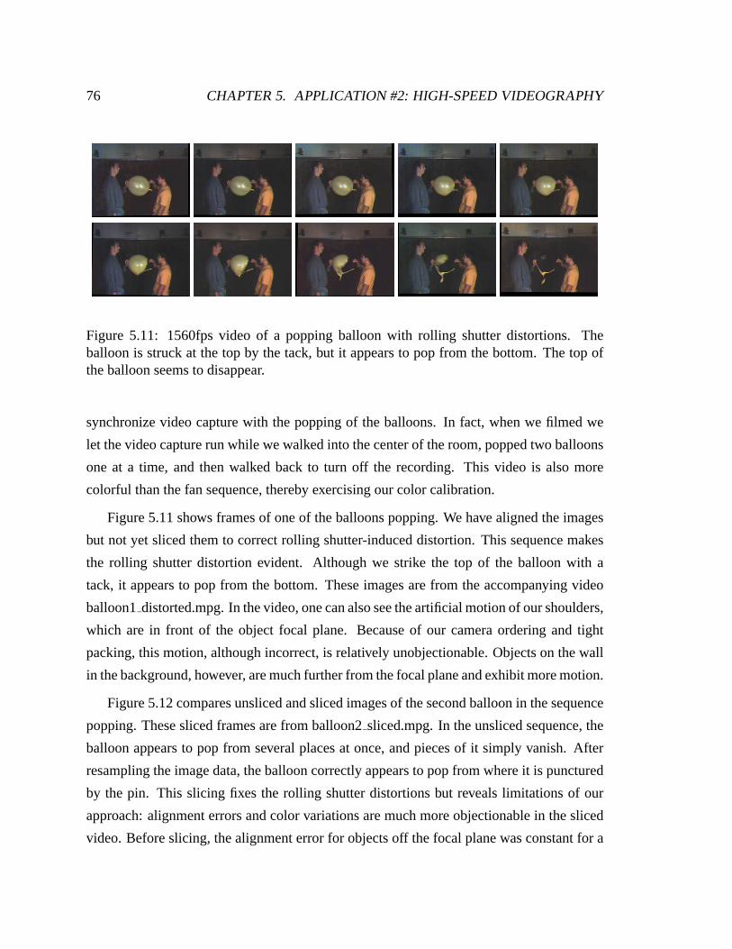
76 CHAPTER 5. APPLICATION #2: HIGH-SPEED VIDEOGRAPHY
Figure 5.11: 1560fps video of a popping balloon with rollingshutter distortions. Theballoon is struck at the top by the tack, but it appears to pop from the bottom. The top ofthe balloon seems to disappear.
synchronize video capture with the popping of the balloons.In fact, when we filmed we
let the video capture run while we walked into the center of the room, popped two balloons
one at a time, and then walked back to turn off the recording. This video is also more
colorful than the fan sequence, thereby exercising our color calibration.
Figure 5.11 shows frames of one of the balloons popping. We have aligned the images
but not yet sliced them to correct rolling shutter-induced distortion. This sequence makes
the rolling shutter distortion evident. Although we strikethe top of the balloon with a
tack, it appears to pop from the bottom. These images are fromthe accompanying video
balloon1distorted.mpg. In the video, one can also see the artificial motion of our shoulders,
which are in front of the object focal plane. Because of our camera ordering and tight
packing, this motion, although incorrect, is relatively unobjectionable. Objects on the wall
in the background, however, are much further from the focal plane and exhibit more motion.
Figure 5.12 compares unsliced and sliced images of the second balloon in the sequence
popping. These sliced frames are from balloon2sliced.mpg. In the unsliced sequence, the
balloon appears to pop from several places at once, and pieces of it simply vanish. After
resampling the image data, the balloon correctly appears topop from where it is punctured
by the pin. This slicing fixes the rolling shutter distortions but reveals limitations of our
approach: alignment errors and color variations are much more objectionable in the sliced
video. Before slicing, the alignment error for objects off the focal plane was constant for a
5.5. RESULTS 77
given depth and varied somewhat smoothly from frame to frame. After slicing, off-plane
objects, especially the background, appear distorted because their alignment error varies
with their vertical position in the image. This distortion pattern scrolls down the image
as the video plays and becomes more obvious. Before slicing, the color variation of each
camera was also confined to a single image in the final high-speed sequence. These short-
lived variations were then averaged by our eyes over severalframes. Once we slice the
images, the color offsets of the images also create a slidingpattern in the video. Note
that some color variations, especially for specular objects, are unavoidable for a multi-
camera system.The reader is once again encouraged to view the videos on the companion
CD to appreciate these effects. The unsliced video of the second balloon popping, bal-
loon2 distorted.mpg, is included for comparison, as well as a continuous video showing
both balloons, balloons.mpg.
The method presented acquires very high-speed video using adensely packed array of
lower frame rate cameras with precisely timed exposure windows. The parallel capture and
compression architecture of the array lets us stream essentially indefinitely. The system
scales to higher frames rates by simply adding more cameras.Inaccuracies correcting the
the temporal offset caused by aligning our rolling shutter images are roughly one sixth
of our frame time and limit the scalability of our array. A more fundamental limit to
the scalability of the system is the minimum integration time of the camera. At 1560fps
capture, the exposure time for our cameras is three times theminimum value. If we scale
beyond three times the current frame rate, the exposure windows of the cameras will begin
to overlap, and our temporal resolution will no longer matchour frame rate.
The possibility of overlapping exposure intervals is a unique feature of our system—no
single camera can expose for longer than the time between frames. If we can use temporal
super-resolution techniques to recover high-speed imagesfrom cameras with overlapping
exposures, we could scale the frame rate even higher than theinverse of the minimum expo-
sure time. As exposure times decrease at very high frame rates, image sensors become light
limited. Typically, high-speed cameras solve this by increasing the size of their pixels and
using very bright lights. Applying temporal super-resolution overlapped high-speed expo-
sures is another possible way to increase the signal-to-noise ratio of a high-speed multi-
camera system. To see if these ideas show promise, I applied the temporal super-resolution

78 CHAPTER 5. APPLICATION #2: HIGH-SPEED VIDEOGRAPHY
Figure 5.12: Comparison of the sliced and unsliced 1560fps balloon pop. The top setof ten pictures are interleaved rolling shutter images. Theballoon appears to pop fromseveral places at once, and pieces of it disappear. Properlyresampling the volume of imagesproduces the lower set of ten images, revealing the true shape of the popping balloon.
method presented by Shechtman [48] to video of a fan filmed with an exposure window
that spanned four high-speed frame times. The temporal alignment process was omitted
because the convolution that relates high-speed frames to our blurred images is known.
Figure 5.13 shows a comparison between the blurred blade, the results of the temporal
super-resolution, and the blade captured in the same lighting with a one frame exposure
window. Encouragingly, the deblurred image becomes sharper and less noisy.
There are several opportunities for improving this work. One is a more sophisticated
alignment method that did not suffer from artificial motion jitter for objects off our assumed
focal plane. Another is combining the high-speed method with other multiple camera ap-
plications. In the next chapter, I will discuss an application that does both–spatiotemporal
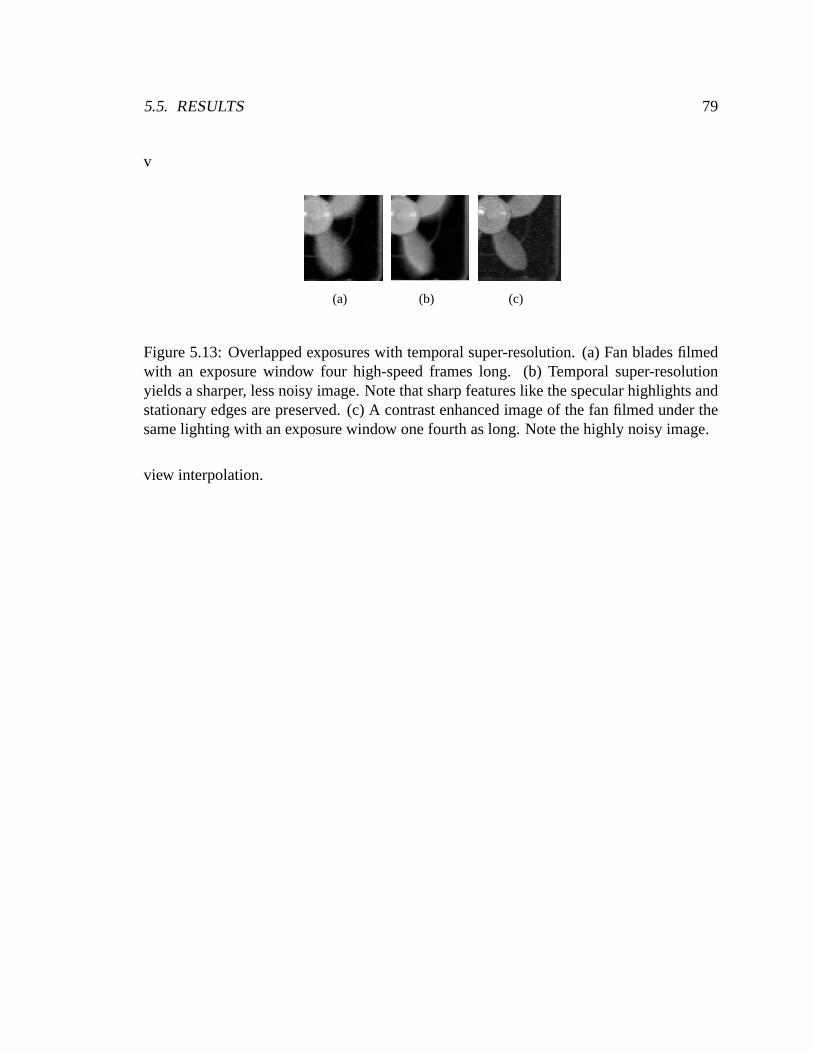
5.5. RESULTS 79
v
(a) (b) (c)
Figure 5.13: Overlapped exposures with temporal super-resolution. (a) Fan blades filmedwith an exposure window four high-speed frames long. (b) Temporal super-resolutionyields a sharper, less noisy image. Note that sharp featureslike the specular highlights andstationary edges are preserved. (c) A contrast enhanced image of the fan filmed under thesame lighting with an exposure window one fourth as long. Note the highly noisy image.
view interpolation.

80 CHAPTER 5. APPLICATION #2: HIGH-SPEED VIDEOGRAPHY
Chapter 6
Application #3: Spatiotemporal View
Interpolation
The synthetic aperture and high-speed videography applications presented in the last two
chapters use an array of cameras, accurate calibration, andprecise camera control to en-
hance performance along a single metric. Nothing prevents us from using this set of tools
to simultaneously improve multiple aspects of camera performance. For example, we could
create a high-speed, synthetic aperture video camera usingstaggered sets of synchronized
cameras spread across the synthetic aperture. Another possibility would be a high dynamic
range, high-resolution video camera constructed from camera clusters, where the cameras
in each cluster have the same field of view but varying exposure times, and their fields of
view abut.
This chapter explores using a dense array of cameras with staggered trigger times to
increase our sampling resolution in both space and time for spatiotemporal view interpola-
tion. We look at the more general problem of optimal samplingpatterns and interpolation
methods for the spatiotemporal volume of images that the camera array records. Large
video camera arrays are typically synchronized, but we showthat staggering camera trig-
gers provides a much richer set of samples on which to base theinterpolation. Richer sam-
pling not only improves the simplest interpolation methods, blending and nearest neighbor,
but also lets one interpolate new space-time views using simple, robust, image-based meth-
ods with simple calibration. We present a novel optical flow method that combines a plane
81
82 CHAPTER 6. APPLICATION #3: SPATIOTEMPORAL VIEW INTERPOLATION
plus parallax framework with knowledge of camera spatial and temporal offsets to generate
flow fields for virtual images at new space-time locations. Wepresent results interpolating
video from a 96-camera light field.
6.1 Introduction
Spatiotemporal view interpolation is the creation of new scene views from locations and
times different from those in the captured set of images. Thesimplest spatiotemporal inter-
polation method is extending light field rendering to video by linearly interpolating in time.
For this reconstruction to work, the image volume must be band-limited. Such prefiltering
adds undesirable blur to the reconstructed images. Even with very large camera arrays, the
sampling density is not sufficiently high to make the blur imperceptible. If the images are
not band-limited, the output exhibits ghosting artifacts.This occurs for large disparities or
temporal motions.
To avoid the conflicting requirements for sharp images with no sampling artifacts, most
image based rendering systems use more sophisticated interpolation schemes based on an
underlying scene model. The simplest method is to estimate motion in an image based
on local information from neighboring views. Other methodsgenerate increasingly so-
phisticated three-dimensional models of the scene. Motionestimation grows less robust
as the “distance” between camera images increases. More complicated models can handle
more widely separated images, but their runtime increases as more global information is
incorporated.
The temporal sampling strategy for an array of cameras–wheneach camera triggers–
affects reconstruction. Traditionally, designers of camera arrays have striven to synchro-
nize their cameras. This often leads to much more temporal motion between camera frames
than parallax motion between neighboring cameras. Instead, staggered triggers are a better
sampling strategy. Improved temporal sampling decreases temporal image motion, allow-
ing us to use simpler, more robust interpolation methods such as optical flow. I will present
a spatiotemporal view interpolation method that uses plane+ parallax calibration to fac-
tor optical flow into parallax and temporal motion components between multiple camera
views.

6.2. PREVIOUS WORK 83
The next section describes previous work in capturing and interpolating between space-
time image samples. I’ll review plane + parallax geometry and our rendering methods, then
describe a framework for determining how best to distributeour camera array samples in
time. Even for basic linear or nearest neighbor, better sampling greatly improves recon-
struction. Finally, I will describe a method for determining spatial and temporal motion
between several views in space and time using optical flow.
6.2 Previous Work
We have already discussed prior work in camera array design and spatial view interpolation.
The Manex Entertainment “Bullet Time” system simulated a physically impossible space-
time camera trajectory through a dynamic scene, but the pathmust be specified in advance.
The cameras capture the views needed for a single camera path. The goal of the work in this
chapter is to investigate how well one could do “Bullet Time” effects as a post-processing
step for a captured set of images without specifying the viewtrajectory in advance.
Spatiotemporal view interpolation depends on sampling strategies and interpolation
methods. Lin and Shum [52] present a maximum camera spacing for static light fields
with a constant depth assumption, and Chai et al. [53] analyzethe minimum spatial sam-
pling rate for static light fields including geometry information. Neither of these works
address temporal sampling rates for video light fields. Vedula et al. [54] and Carceroni
and Kutulakos [55] present methods for interpolating new space-time views using arrays of
synchronized cameras with coincident triggers. They explicitly solve for scene reflectance,
structure and motion. By contrast, my system exploits large numbers of inexpensive sensors
and improved temporal sampling to reduce spatiotemporal view interpolation to a simpler,
image-based task.
6.3 Calibration and Rendering
For this work, the cameras are assembled either in a line or a plane so we can take advantage
of plane + parallax calibration. Because this calibration iscentral to this work, I will briefly
review it. Starting with a planar array of cameras, we align all of the camera images to

84 CHAPTER 6. APPLICATION #3: SPATIOTEMPORAL VIEW INTERPOLATION
a fronto-parallel reference plane using 2D image homographies. In the aligned images,
points in the scene lying on the reference plane show no parallax between views. Points off
the reference plane will have a parallax of∆p = ∆x·d, where∆x is the vector fromC0 toC1
in the camera plane, andd is the relative depth of the point. This has two implications:
• Once we have aligned images to a common reference plane, the parallax between
aligned images of a single point off the reference plane is enough to determine the
relative locations in the camera plane of all of the cameras.As shown by Vaish et al.
[7], the camera displacements can be computed robustly frommultiple measurements
using a rank-1 factorization via SVD.
• Given the relative camera displacements in the camera plane, the relative depth of a
point in one view suffices to predict its location in all otherviews. This provides a
powerful way to combine data from many images.
Once again, we will align all of our input images to a reference plane. The aligned
images provide a common space in which to analyze and combineviews. Levoy and Han-
rahan represent light fields with a two-plane(u,v,s, t) parametrization. For a planar array of
cameras, the aligned images correspond(s, t) parameterized images for light field render-
ing, so measuring motion in the reference plane indicates how much aliasing we would see
in reconstructed light field images. We will use this framework both to analyze temporal
sampling requirements and for determining image flow between neighboring space-time
views.
Aligning our images to a reference plane automatically corrects for geometric variations
in our cameras (excluding translations out of the camera plane and radial distortion, which
we have found to be negligible for our application). The aligned images are generally off-
axis projections, which are visually disturbing. This is clear from the aligned views of
the calibration target in figure 4.7–the reference plane will always appear fronto-parallel,
regardless of the camera position.
The transformation that we need for rendering corrects the off-axis projection and is
equivalent to taking a picture of the aligned plane from the virtual camera position. Plane
+ parallax calibration does not provide enough informationto do this. If we fix the relative
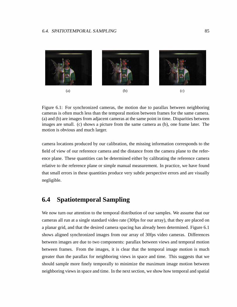
6.4. SPATIOTEMPORAL SAMPLING 85
(a) (b) (c)
Figure 6.1: For synchronized cameras, the motion due to parallax between neighboringcameras is often much less than the temporal motion between frames for the same camera.(a) and (b) are images from adjacent cameras at the same pointin time. Disparities betweenimages are small. (c) shows a picture from the same camera as (b), one frame later. Themotion is obvious and much larger.
camera locations produced by our calibration, the missing information corresponds to the
field of view of our reference camera and the distance from thecamera plane to the refer-
ence plane. These quantities can be determined either by calibrating the reference camera
relative to the reference plane or simple manual measurement. In practice, we have found
that small errors in these quantities produce very subtle perspective errors and are visually
negligible.
6.4 Spatiotemporal Sampling
We now turn our attention to the temporal distribution of oursamples. We assume that our
cameras all run at a single standard video rate (30fps for ourarray), that they are placed on
a planar grid, and that the desired camera spacing has already been determined. Figure 6.1
shows aligned synchronized images from our array of 30fps video cameras. Differences
between images are due to two components: parallax between views and temporal motion
between frames. From the images, it is clear that the temporal image motion is much
greater than the parallax for neighboring views in space andtime. This suggests that we
should sample more finely temporally to minimize the maximumimage motion between
neighboring views in space and time. In the next section, we show how temporal and spatial
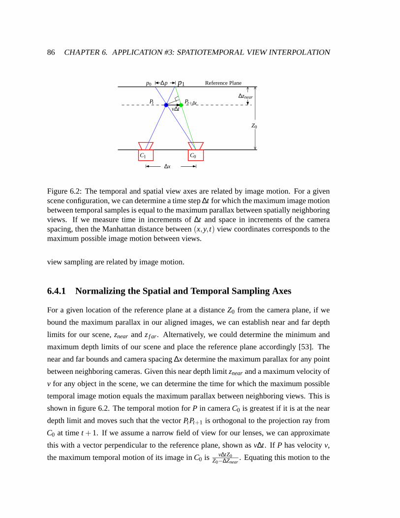
86 CHAPTER 6. APPLICATION #3: SPATIOTEMPORAL VIEW INTERPOLATION
PlaneReference
v∆tPt Pt+∆t
∆x
p0 p1∆p
Z0
∆znear
C1 C0
Figure 6.2: The temporal and spatial view axes are related byimage motion. For a givenscene configuration, we can determine a time step∆t for which the maximum image motionbetween temporal samples is equal to the maximum parallax between spatially neighboringviews. If we measure time in increments of∆t and space in increments of the cameraspacing, then the Manhattan distance between(x,y, t) view coordinates corresponds to themaximum possible image motion between views.
view sampling are related by image motion.
6.4.1 Normalizing the Spatial and Temporal Sampling Axes
For a given location of the reference plane at a distanceZ0 from the camera plane, if we
bound the maximum parallax in our aligned images, we can establish near and far depth
limits for our scene,znear andz f ar. Alternatively, we could determine the minimum and
maximum depth limits of our scene and place the reference plane accordingly [53]. The
near and far bounds and camera spacing∆x determine the maximum parallax for any point
between neighboring cameras. Given this near depth limitznear and a maximum velocity of
v for any object in the scene, we can determine the time for which the maximum possible
temporal image motion equals the maximum parallax between neighboring views. This is
shown in figure 6.2. The temporal motion forP in cameraC0 is greatest if it is at the near
depth limit and moves such that the vectorPtPt+1 is orthogonal to the projection ray from
C0 at timet + 1. If we assume a narrow field of view for our lenses, we can approximate
this with a vector perpendicular to the reference plane, shown asv∆t. If P has velocityv,
the maximum temporal motion of its image inC0 is v∆tZ0Z0−∆Znear
. Equating this motion to the
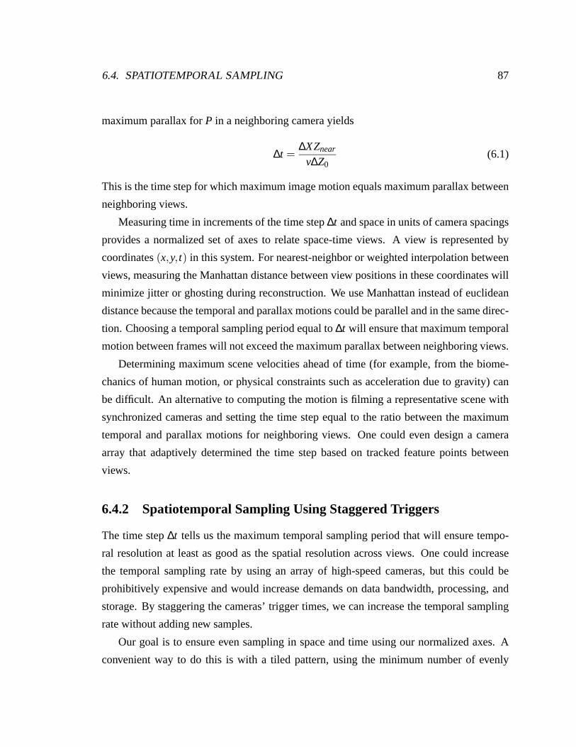
6.4. SPATIOTEMPORAL SAMPLING 87
maximum parallax forP in a neighboring camera yields
∆t =∆XZnear
v∆Z0(6.1)
This is the time step for which maximum image motion equals maximum parallax between
neighboring views.
Measuring time in increments of the time step∆t and space in units of camera spacings
provides a normalized set of axes to relate space-time views. A view is represented by
coordinates(x,y, t) in this system. For nearest-neighbor or weighted interpolation between
views, measuring the Manhattan distance between view positions in these coordinates will
minimize jitter or ghosting during reconstruction. We use Manhattan instead of euclidean
distance because the temporal and parallax motions could beparallel and in the same direc-
tion. Choosing a temporal sampling period equal to∆t will ensure that maximum temporal
motion between frames will not exceed the maximum parallax between neighboring views.
Determining maximum scene velocities ahead of time (for example, from the biome-
chanics of human motion, or physical constraints such as acceleration due to gravity) can
be difficult. An alternative to computing the motion is filming a representative scene with
synchronized cameras and setting the time step equal to the ratio between the maximum
temporal and parallax motions for neighboring views. One could even design a camera
array that adaptively determined the time step based on tracked feature points between
views.
6.4.2 Spatiotemporal Sampling Using Staggered Triggers
The time step∆t tells us the maximum temporal sampling period that will ensure tempo-
ral resolution at least as good as the spatial resolution across views. One could increase
the temporal sampling rate by using an array of high-speed cameras, but this could be
prohibitively expensive and would increase demands on databandwidth, processing, and
storage. By staggering the cameras’ trigger times, we can increase the temporal sampling
rate without adding new samples.
Our goal is to ensure even sampling in space and time using ournormalized axes. A
convenient way to do this is with a tiled pattern, using the minimum number of evenly
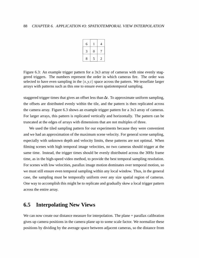
88 CHAPTER 6. APPLICATION #3: SPATIOTEMPORAL VIEW INTERPOLATION
0
1
2
3
4
5
6
7
8
Figure 6.3: An example trigger pattern for a 3x3 array of cameras with nine evenly stag-gered triggers. The numbers represent the order in which cameras fire. The order wasselected to have even sampling in the(x,y, t) space across the pattern. We tessellate largerarrays with patterns such as this one to ensure even spatiotemporal sampling.
staggered trigger times that gives an offset less than∆t. To approximate uniform sampling,
the offsets are distributed evenly within the tile, and the pattern is then replicated across
the camera array. Figure 6.3 shows an example trigger pattern for a 3x3 array of cameras.
For larger arrays, this pattern is replicated vertically and horizontally. The pattern can be
truncated at the edges of arrays with dimensions that are notmultiples of three.
We used the tiled sampling pattern for our experiments because they were convenient
and we had an approximation of the maximum scene velocity. For general scene sampling,
especially with unknown depth and velocity limits, these patterns are not optimal. When
filming scenes with high temporal image velocities, no two cameras should trigger at the
same time. Instead, the trigger times should be evenly distributed across the 30Hz frame
time, as in the high-speed video method, to provide the best temporal sampling resolution.
For scenes with low velocities, parallax image motion dominates over temporal motion, so
we must still ensure even temporal sampling within any localwindow. Thus, in the general
case, the sampling must be temporally uniform over any size spatial region of cameras.
One way to accomplish this might be to replicate and gradually skew a local trigger pattern
across the entire array.
6.5 Interpolating New Views
We can now create our distance measure for interpolation. The plane + parallax calibration
gives up camera positions in the camera plane up to some scalefactor. We normalize these
positions by dividing by the average space between adjacentcameras, so the distance from

6.5. INTERPOLATING NEW VIEWS 89
a camera to its horizontal and vertical neighbors is approximately one. Let(x,y) be the
position of each camera in these normalized coordinates, and let t be the time at which a
given image is acquired, measured in time steps of∆t. Because we have chosen a time step
that sets the maximum parallax between views equal to the maximum temporal motion
between time steps, the euclidean distance between the(x,y, t) coordinates representing
two views is a valid measure of the maximum possible motion between the two images.
The simplest way we could interpolate new views would be to use nearest neighbors
as in the high-speed videography method of chapter 5. This method produces accept-
able results, but as points move off the reference plane, their images jitter due to parallax
between views. The perceived jitter can be reduced using interpolation between several
nearby views. To determine which images to blend and how to weight them, we compute
a Delauney tessellation of our captured image coordinates.For a new view(x,y, t), we
find the tetrahedron of images in the tessellation containing the view and blend the images
at its vertices using their barycentric coordinates as weights. Using this tessellation and
barycentric weighting ensures that our blending varies smoothly as we move the virtual
viewpoint. As we leave one tetrahedron, the weights of dropped vertices go to zero. Our
temporal sampling pattern is periodic in time, so we only need to compute the tessellation
for three 30Hz sampling periods to compute the weights for anarbitrarily long sequence.
Figure 6.4 shows the benefits of improved temporal sampling.In this experiment, we
used a 12x8 array of 30fps video cameras similar to that shownin figure 3.4 to film me
heading a soccer ball. The cameras were triggered accordingto the pattern in figure 6.3,
tiled across the array. We then generated 270fps interpolated video using several methods.
First, we used a cross-dissolve between sequential frames at one camera to simulate linear
interpolation for a synchronized array. The motion of the soccer ball between captured
frames is completely absent. Next, we used nearest-neighbor interpolation, which assem-
bles a video sequence using video captured at the proper timefrom neighboring cameras.
This produces sharp images and captures the path of the ball,but the motion is jittered due
to parallax between views. Finally, we used the barycentricweighted averaging described
previously. This reduces the ball’s motion jitter but introduces ghosting.
Staggering the cameras clearly improves our temporal resolution and results in much
better results even for simple nearest-neighbor and weighted interpolation. Because our
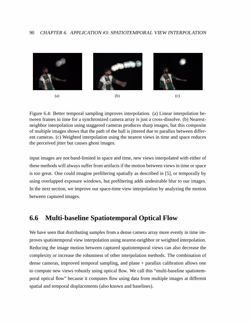
90 CHAPTER 6. APPLICATION #3: SPATIOTEMPORAL VIEW INTERPOLATION
(a) (b) (c)
Figure 6.4: Better temporal sampling improves interpolation. (a) Linear interpolation be-tween frames in time for a synchronized camera array is just across-dissolve. (b) Nearest-neighbor interpolation using staggered cameras produces sharp images, but this compositeof multiple images shows that the path of the ball is jittereddue to parallax between differ-ent cameras. (c) Weighted interpolation using the nearest views in time and space reducesthe perceived jitter but causes ghost images.
input images are not band-limited in space and time, new views interpolated with either of
these methods will always suffer from artifacts if the motion between views in time or space
is too great. One could imagine prefiltering spatially as described in [5], or temporally by
using overlapped exposure windows, but prefiltering adds undesirable blur to our images.
In the next section, we improve our space-time view interpolation by analyzing the motion
between captured images.
6.6 Multi-baseline Spatiotemporal Optical Flow
We have seen that distributing samples from a dense camera array more evenly in time im-
proves spatiotemporal view interpolation using nearest-neighbor or weighted interpolation.
Reducing the image motion between captured spatiotemporal views can also decrease the
complexity or increase the robustness of other interpolation methods. The combination of
dense cameras, improved temporal sampling, and plane + parallax calibration allows one
to compute new views robustly using optical flow. We call this“multi-baseline spatiotem-
poral optical flow” because it computes flow using data from multiple images at different
spatial and temporal displacements (also known and baselines).
6.6. MULTI-BASELINE SPATIOTEMPORAL OPTICAL FLOW 91
We extended Black and Anandan’s optical flow method [56] usingcode available on the
author’s web site. Their algorithm is known to handle violations of the intensity constancy
and smoothness assumptions well using robust estimation. It uses a standard hierarchical
framework to capture large image motions, but can fail due tomasking when small regions
of the scene move very differently from a dominant background [57]. For our 30fps syn-
chronized juggling sequence, the algorithm succeeded between cameras at the same time
but failed between subsequent frames from the same camera. The motion of the small
juggled balls was masked by the stationary background. Oncewe retimed the cameras,
the motion of the balls was greatly reduced, and the algorithm computed flow accurately
between pairs of images captured at neighboring locations and time steps.
Our modified spatiotemporal optical flow algorithm has two novel features. First, we
solve for a flow field at the(x,y, t) location of our desired virtual view. This was inspired
by the bidirectional flow of Kang et al. [58], who observe thatfor view interpolation, com-
puting the flow at the new view position instead of either source image handles degenerate
flow cases better and avoids the hole-filling problems of forward-warping when creating
new views. They use this to compute flow at a frame halfway between two images in a
video sequence. Typically, optical flow methods will compute flow between two images by
iteratively warping one towards the other. They calculate flow at the halfway point between
two frames by assuming symmetric flow and iteratively warping both images to the mid-
point. We extend the method to compute flow at a desired view inour normalized(x,y, t)
view space. We iteratively warp the nearest four captured images toward the virtual view
and minimize the weighted sum of the robust pairwise data errors and a robust smoothness
error.
Motion cannot be modeled consistently for four images at different space-time locations
using just horizontal and vertical image flow. The second component of this algorithm is
simultaneously accounting for parallax and temporal motion. We decompose optical flow
into the traditional two-dimensional temporal flow plus a third flow term for relative depth
that accounts for parallax between views. The standard intensity constancy equation for
optical flow is
I(i, j, t) = I(i+uδ t, j + vδ t, t +δ t) (6.2)
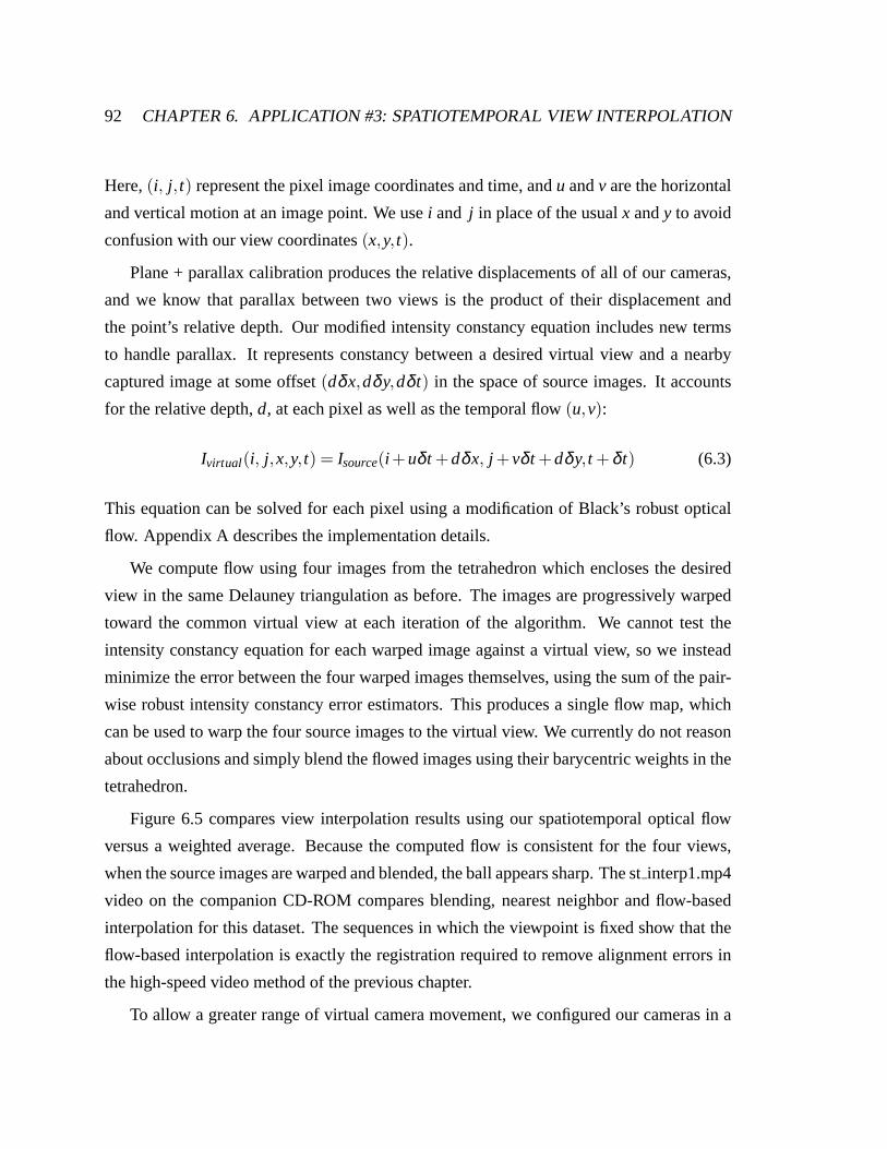
92 CHAPTER 6. APPLICATION #3: SPATIOTEMPORAL VIEW INTERPOLATION
Here,(i, j, t) represent the pixel image coordinates and time, andu andv are the horizontal
and vertical motion at an image point. We usei and j in place of the usualx andy to avoid
confusion with our view coordinates(x,y, t).
Plane + parallax calibration produces the relative displacements of all of our cameras,
and we know that parallax between two views is the product of their displacement and
the point’s relative depth. Our modified intensity constancy equation includes new terms
to handle parallax. It represents constancy between a desired virtual view and a nearby
captured image at some offset(dδx,dδy,dδ t) in the space of source images. It accounts
for the relative depth,d, at each pixel as well as the temporal flow(u,v):
Ivirtual(i, j,x,y, t) = Isource(i+uδ t +dδx, j + vδ t +dδy, t +δ t) (6.3)
This equation can be solved for each pixel using a modification of Black’s robust optical
flow. Appendix A describes the implementation details.
We compute flow using four images from the tetrahedron which encloses the desired
view in the same Delauney triangulation as before. The images are progressively warped
toward the common virtual view at each iteration of the algorithm. We cannot test the
intensity constancy equation for each warped image againsta virtual view, so we instead
minimize the error between the four warped images themselves, using the sum of the pair-
wise robust intensity constancy error estimators. This produces a single flow map, which
can be used to warp the four source images to the virtual view.We currently do not reason
about occlusions and simply blend the flowed images using their barycentric weights in the
tetrahedron.
Figure 6.5 compares view interpolation results using our spatiotemporal optical flow
versus a weighted average. Because the computed flow is consistent for the four views,
when the source images are warped and blended, the ball appears sharp. The stinterp1.mp4
video on the companion CD-ROM compares blending, nearest neighbor and flow-based
interpolation for this dataset. The sequences in which the viewpoint is fixed show that the
flow-based interpolation is exactly the registration required to remove alignment errors in
the high-speed video method of the previous chapter.
To allow a greater range of virtual camera movement, we configured our cameras in a
6.7. DISCUSSION 93
(a) (b)
Figure 6.5: View interpolation using space-time optical flow. (a) Interpolated 270fps videousing weighted average of four source images. (b) Interpolated 270fps video using opticalflow. The four source images were warped according to the computed flow and then aver-aged using the same weights as in image a. No double images arepresent because parallaxand motion for the ball were correctly recovered.
30 wide by 3 tall array. We used the same 3x3 trigger ordering,tiled across the array. In
st interp2.mp4 on the CD-ROM, we show another soccer sequence inwhich we alternate
smoothly between rendering from one view position at 270fpsto freezing time and render-
ing from novel viewing positions. Figure 6.6 shows twenty frames with a slowly varying
viewing positions and times. Figure 6.7 shows five frames spanning the spatial viewing
range of the array.
6.7 Discussion
Our multiple camera array allows us to control the image samples that are recorded from the
spatiotemporal volume a scene generates, and the sampling pattern chosen greatly affects
the complexity of the view interpolation task. While in theory it is possible to simply
resample a linear filtered version of the samples to generatenew views, even with large
numbers of inexpensive cameras, it seems unlikely one couldobtain high enough sampling
density to prevent either blurred images or ghosting artifacts. Instead, the correct placement
94 CHAPTER 6. APPLICATION #3: SPATIOTEMPORAL VIEW INTERPOLATION
of samples allows the use of simpler modeling approaches rather than none at all. The key
question is, how sophisticated a model is needed and what sampling basis allows the most
robust modeling methods to be used to construct a desired view?
For many interpolation methods, minimizing image motion leads to better quality view
synthesis, so we use minimizing image motion to guide our sample placement. Given our
relatively planar camera array, we use a very simple plane + parallax calibration for inter-
polation in space. For images aligned to a reference plane, spatial view motion results in
parallax for points not on the reference plane. This motion must be balanced against tem-
poral image motion. In our camera array this disparity motion is modest between adjacent
cameras, and is much smaller than the true motion from frame to frame.
Staggering camera trigger in time distributes samples to reduce temporal image motion
between neighboring views without adding new samples. In a way staggered time sampling
is never a bad sampling strategy. Clearly the denser time samples help for scenes with high
image motion. For scenes with small motion, the denser time samples do no harm. Since
the true image motion is small, it is easy to estimate the image at any intermediate time, un-
doing the time skew adds little error. Since the spatial sampling density remains unchanged,
it does not change the view interpolation problem at all. Better temporal sampling lets us
apply relatively simple, fairly robust models like opticalflow to view interpolation in time
and space. We solve for temporal image motion and image motion due to parallax which
improves our interpolation.
Because our flow-based view interpolation methods are local,the constraints on the
camera timings are also local. They need to sample evenly in every local neighborhood.
We use a simple tessellated pattern with locally uniform sampling at the interior and across
boundaries. Algorithms that aggregate data from an entire array of cameras will benefit
from different time stagger patterns and raises the interesting question of finding an optimal
sampling pattern for a few of the more sophisticated model-based methods.
While it is tempting to construct ordered dither patterns to generate unique trigger times
for all cameras there is a tension between staggered shutters to increase temporal resolution
and models that exploit the rigid-body nature of a single time slice. This seems to be an
exciting area for further research.
Staggered trigger times for camera arrays increase temporal resolution with no extra
6.7. DISCUSSION 95
cost in hardware or bandwidth, but have other limits. One fundamental limit is the num-
ber of photons imaged by the cameras if the exposure windows are non-overlapping. The
aperture time for each camera is set to be equal to the smallest time difference between the
cameras. While this minimizes unintended motion blur, allowing sharp images in “Bul-
let time” camera motion, at some point the number of photons in the scene will be too
small, and the resulting image signal to noise ratio will begin to increase. This gives rise
to another dimension that needs to be explored—optimizing the relation between the mini-
mum spacing between time samples and the aperture of the cameras. As mentioned earlier,
Shechtman et al. [48] have done some promising work in this area, using multiple un-
synchronized cameras with overlapping exposures to eliminate motion blur and motion
aliasing in a video sequence.
For our image-based methods, uniform spatiotemporal sampling limits image motion
and enhances the performance of our interpolation methods.We analyzed spatiotemporal
sampling from the perspective of interpolation with a constant depth assumption and related
the temporal and spatial axes with maximum image motions dueto parallax and time. That
constant-depth assumption is one of the limitations of thiswork. In the future, I would
like to enable more general scene geometries. The spatiotemporal optical flow method
generates significantly better results than weighted averaging, but still suffers from the
standard vulnerabilities of optical flow, especially occlusions and masking.

96 CHAPTER 6. APPLICATION #3: SPATIOTEMPORAL VIEW INTERPOLATION
(7.47,192.6) (7.00,194.4) (6.53,196.3) (6.07,198.1) (5.60,200.0)
(5.13,201.9) (4.67,203.7) (4.20,205.6) (3.73,207.4) (3.27,209.3)
(2.80,211.1) (2.33,213.0) (1.87,214.8) (1.40,216.7) (0.93,218.5)
(0.47,220.4) (0,222.2) (0,224.1) (0,225.9) (0,227.8)
Figure 6.6: Twenty sequential frames from an interpolated video sequence demonstrat-ing slowly varying view positions and times. The input data were captured using a 30x3array of cameras with nine different trigger times. All views shown are synthesized. Be-neath each image are the (x,t) view coordinates, with x in units of average camera spacings(roughly three inches) and t in milliseconds. Motion is moreevident looking across rowsor along diagonals from top left to bottom right.
-15.0 -8.2 0.47 7.23 14.0
Figure 6.7: Five synthesized views showing the spatial viewing range for the 30x3 config-uration. View spatial coordinate is again in units of cameraspacings, roughly three inches.
Chapter 7
Conclusions
Digital video cameras are becoming cheap and widespread, creating new opportunities for
increased imaging performance. Researchers in this space encounter several obstacles. For
system designers, large video camera arrays generate data at rates that overwhelm com-
modity personal computers and storage media. Inexpensive commodity cameras do not
offer the degree of control or flexibility required for research. Assuming some system for
collecting data from many cameras, researchers must devisecalibration methods that scale
to large numbers of cameras, and vision and graphics algorithms that robustly account for
the lower image quality and more varied geometric and radiometric properties of inexpen-
sive camera arrays.
The architecture in this thesis addresses the issues of scale in large camera array design.
It exploits CMOS image sensors, IEEE1394 communication and MPEG video compression
to control and capture video from very large numbers of cameras to a few PCs. A flexible
mounting system lets us explore many different configurations and applications. I have
shown three applications demonstrating that we can effectively combine data from many
inexpensive sensors to increase imaging performance.
Although synthetic aperture photography has been done withstatic scenes before, we
were the first to capture synthetic aperture videos or to use the technique to look through
partial occluders. Our live synthetic aperture system withinteractive focal plane adjustment
also shows the value of low-level image processing power at the cameras.
The high-speed videography method increases the effectivetemporal sampling rate of
97
98 CHAPTER 7. CONCLUSIONS
our system by staggering the trigger times of the cameras. Wecan compensate for the
electronic rolling shutter in many low-end sensors by jittering the camera triggers and re-
sampling their output. We have pushed this technique up to 1560fps video using 52 tightly
packed, 30fps cameras. The parallel compression in the array lets us stream continuously
at this frame rate.
The spatiotemporal view interpolation system I propose simultaneously extends imag-
ing performance along multiple axes–view position and time. It shows that with inex-
pensive cameras, we can reduce view interpolation of dynamic scenes from estimating
three-dimensional structure and motion to determining parallax and two-dimensional im-
age velocities. Much of this gain is due to improved samplingfrom staggered trigger times,
which minimizes image motion between captured views and enables optical-flow based
algorithms. The multi-baseline, spatiotemporal optical flow method not only presents a
simple framework for synthesizing new virtual views, but also demonstrates that the cali-
bration is adequate for vision algorithms like optical flow,which are sensitive to noise and
radiometric camera variations.
We have shown a video capture system for large arrays of inexpensive cameras and
applications proving that we can use these cameras for interesting high-performance imag-
ing, computer vision, and graphics applications. Where do wego from here? Our recent
experiments with real-time applications using the camera array have produced encouraging
results, but performance limits imposed by the architecture are already apparent. We can
do low-level image processing at each camera, but image datafrom multiple cameras can
only be combined at the host PC. Thus, the host PCs are the bottleneck for our live syn-
thetic aperture system. The same would be true of any on-the-fly light field compression
method that accounts for data redundancy between cameras. Future designs should clearly
allow data to flow between cameras. That said, we must developapplications before we
can determine the performance needs for a next generation array, and the array as is has
already proved to be a valuable tool in that research.
SAP and high-speed videography are but two of the high-x methods enumerated in
chapter 2, and it would be interesting to pursue others. As part of the on-going research
effort involving the camera array, we are currently exploring the high-resolution approach
using cameras with abutting fields of view. We hope to take advantage of the per-camera
99
processing to individually meter each camera and extend thedynamic range of the mosaic,
too. Some global communication to ensure smooth transitions in metering across the array
might be necessary.
There still remain several other untapped high-x dimensions: dynamic range, depth of
field, spectral resolution, low noise, and so on. One question raised by the high-x appli-
cations is, when can a cluster of cameras outperform a single, more expensive camera?
For many applications, it will depend on the economics and quality of inexpensive sensors
compared to the available performance gain of using many cameras. For example, because
the noise reduction from averaging images fromn cameras grows only assqrt(n), if inex-
pensive cameras have much worse noise performance than the expensive alternative (due
to poor optics, more dark current, and so on), they will be unable to affordably close the
gap. By contrast, for high-resolution imaging using cameraswith abutting fields of view,
resolution grows linearly with the number of cameras, whilecost most likely grows much
faster when increasing the resolution of a single camera. For this reason, I would expect
the multiple camera approach to be superior.
For other applications, the consequences of imaging with multiple cameras will fun-
damentally limit performance regardless of sensor qualityor cost. For example, even if
our high-speed videography method were not limited by the poor light-gathering ability
of inexpensive sensors, we would still have to contend with errors caused by the multiple
camera centers of projection. With perfect radiometric camera calibration, we will still
see differences between images from adjacent cameras due tospecularities and occlusions.
These types are artifacts are unavoidable. Optical methodsto ensure a common center of
projection might be acceptable for some applications, but not for high-speed videography
because they reduce the light that reaches each camera.
Attempting to outperform single, high-end cameras will prove fruitful for some appli-
cations, but an even richer area to explore is performance gains that are impossible with a
single camera. View interpolation itself is one example. Another is the synthetic aperture
matting technique I mention in chapter 4. Summing contributions only from pixels in the
input images that see through the occluder eliminates the foreground instead of blurring it
away and produces images with greater contrast. This nonlinear operation would be impos-
sible with a single large-aperture camera. Surely there exist other opportunities for these
100 CHAPTER 7. CONCLUSIONS
sorts of advances.
The possibilities for improved imaging using arrays of inexpensive cameras are vast,
but the tools for exploring them are rare. When I started this project, I did not anticipate
that completely reconfiguring an array of one hundred cameras for new applications would
someday become a common and undaunting task. I hope this thesis has convinced the
reader not only that we can provide the control, capture and calibration capabilities neces-
sary to easily experiment with hundreds of cameras, but alsothat these experiments will
yield rich results.

Appendix A
Spatiotemporal optical flow
implementation
In this appendix, I will describe in detail how we solve for spatiotemporal optical flow at
virtual view locations. To review, the goal of multibaseline spatiotemporal optical flow is to
determine components of image motion due to temporal scene motion and parallax between
views of a scene from different positions and times. To make view interpolation simple,
we solve for this flow for pixels in the image at the virtual viewing position and time. Our
views are parametrized by(x,y, t), where(x,y) is the location in our plane of cameras, and
t is the time the image was captured. We use four source views tocompute flow because
that is the minimum number to enclose a given virtual view in our 3D space-time view
coordinates.
We assume that our cameras all lie in a plane and use plane + parallax calibration to
determine the displacements,xi, between the cameras and some reference camera. Note
that although we use a reference camera for the displacements (typically a central camera),
our algorithm is still truly multi-view, considering all cameras equally, because only the
relative displacements between cameras matter. We align all of the images from all cameras
to a common reference plane using planar homographies. In the aligned images, for two
cameras separated in the camera plane by some relative displacementx, the parallax for a
given point at relative depthw is justwx.
We represent temporal scene motion by its two-dimensional projection(u,v) onto the
101
102 APPENDIX A. SPATIOTEMPORAL OPTICAL FLOW IMPLEMENTATION
image plane, similarly to traditional optical flow. Especially for cameras aligned on a plane,
estimating motion on the z-axis can be ill-conditioned. Because the camera trigger times
are deliberately offset to increase the temporal sampling resolution and ensure that for any
virtual view there are several captured views from nearby locations and times, the combined
motion due temporal and spatial view changes is minimized.
Multibaseline spatiotemporal optical flow estimates the instantaneous(u,v,w) image
flow for each pixel in a virtual view at position and time(x,y, t). It is called multibase-
line because it considers multiple source images for each virtual view, and the spatial and
temporal distances from the arbitrary virtual view to each of the nearby captured ones are
generally different. For each pixel(i, j) in the virtual view, we attempt to solve the follow-
ing equation with respect to each source image:
Ivirtual(i, j,x,y, t) = Isource(i+uδ t +wδx, j + vδ t +wδy, t +δ t)
Optical flow methods traditionally compute a flow error metric by warping one image to-
ward the other based on the computed flow and measuring their difference. Because the
virtual image does not exist, we cannot directly compare it to each warped source image.
Instead, we measure the accuracy of the computed flow by warping the four nearby space-
time views to the virtual view and comparing them to each other.
At this point, we adopt the robust optical flow framework described by Michael Black
in [56]. He determines flow in one image with respect to another by minimizing a robust
error function with data conservation and spatial smoothness terms. The data conservation
term at each pixel is derived from the intensity constancy equation:
ED = ρ1(Ixu+ Iyv+ It ,σ1)
Here,Ix, Iy and It are the spatial and temporal image derivatives, andρ1(err,σ) is some
error estimator.ρ1(x) = x2 would correspond to squared error estimation. The spatial
coherence term measures the spatial derivative of the computed flow at each pixel:
ES = λ ∑n∈G
(ρ2(u−un,σ2)+ρ2(v− vn,σ2))
103
whereG are the north, south, east and west neighboring pixels, andun and uv are the
computed flow for pixel n in that set.λ sets the relative weight of the smoothness term
versus the data term.
Motion discontinuities and occlusions violate assumptions of smoothness and intensity
constancy, and create outlier errors that deviate greatly from the Gaussian measurement
error assumed by least squares. These outliers have inordinately large influences on squared
errors. Black introduces robust error estimators that reduce the effect of these outliers.
For his flow implementation, he uses the Lorentzian, whose value ρ(x,σ) and derivative
ψ(x,σ) with respect to a measured error x are:
ρσ (x) = log
(
1+12
( xσ
)2)
ψσ (x) =2x
2σ2 + x2
σ is a scale factor related to the expected values of inliers and outliers.
We too use the Lorentzian estimator. Now, we can formalize our error metric. Although
we solve for flow using multiple source images, we compute that flow for pixels in a single
virtual image. Thus, the spatial coherence error termES is unchanged. Our data coherence
term must measure errors between four source images warped to the virtual view accord-
ing to our three-component flow(u,v,w). To use gradient-based optical flow, we need to
compute temporal derivatives between images, so we measurethe sum of pairwise robust
errors between warped images. Here, we define three new quantities for each source view
relative to the virtual view.αn = tn − tv is the temporal offset from the virtual image cap-
tured at timetv to source imageIn captured at timetn. (βnx,βny) = (xn − xv,yn − yv) is the
relative displacement in the camera plane from the virtual view to source viewIn. The data
conservation error term at each pixel is:
ED = ∑m6=n
ρ1
(
Ixm,n(u(αm −αn)+w(βmx −βnx))+ Iym,n(v(αm −αn)
+w(βmy −βny))+ Itm,n ,σ1
)
Here,Ixm,n is the average of the horizontal image spatial derivatives in imageIn andIm at
104 APPENDIX A. SPATIOTEMPORAL OPTICAL FLOW IMPLEMENTATION
the pixel, and likewise for the vertical spatial derivativeIym,n . Itm,n is simplyIm − In for each
pixel.
Now that we have defined robust error functions for multibaseline spatiotemporal op-
tical flow, all that remains is to solve for(u,v,w) at each pixel to minimize the error. We
modified Black’s publicly available code that calculates flowhierarchically using grad-
uated non-convexity (GNC) and successive over-relaxation (SOR). Hierarchical methods
filter and downsample the input images in order to capture large motions using a gradient-
based framework. GNC replaces a non-convex error term with aconvex one to guarantee
a global minimum, then iterates while adjusting the error term steadily towards the desired
non-convex one. Successive over-relaxation is an iterative method for the partial differ-
ential equations the result from the data consistency and smoothness terms. Readers are
referred to [56] more details.
The iterative SOR update equation for minimizingE = ED + ES at stepn + 1 has the
same form as in Black’s work, but we have to update three terms for flow:
u(n+1) = u(n)−ω1
T (u)
∂E∂u
v(n+1) = v(n)−ω1
T (v)∂E∂v
w(n+1) = w(n)−ω1
T (w)
∂E∂w
where 0< ω < 2 is a parameter used to over correct the estimates foru, v, andw at each
step and speed convergence. The first partial derivatives ofE with respect tou, v, andw are
∂E∂u
=
(
∑m6=n
Ixm,n(αm −αn)ψ1(errm,n,σ1)
)
+λ ∑n∈G
ψ2(u−un,σ2)
∂E∂v
=
(
∑m6=n
Iym,n(αm −αn)ψ1(errm,n,σ1)
)
+λ ∑n∈G
ψ2(v− vn,σ2)

105
∂E∂w
=
(
∑m6=n
(Ixm,n(βmx −βnx)ψ1(errm,n)+ Iym,n(βmy −βny)ψ1(errm,n))
)
+λ ∑n∈G
ψ2(w−wn,σ2)
whereG as before are north, south, east and west neighbors of each pixel, m andn are
from the set{1,2,3,4} of input images, anderrm,n is the intensity constancy error:
errm,n = Ixm,n(u(αm −αn)+w(βmx −βnx))+ Iym,n(v(αm −αn)+w(βmy −βny))+ Itm,n
T(u), T(v), and T(w) are upper bounds on the second partial derivatives of E:
T (u) =
(
∑m6=n
I2xm,n
(αm −αn)2
σ21
)
+4λσ2
2
T (v) =
(
∑m6=n
I2ym,n
(αm −αn)2
σ21
)
+4λσ2
2
T (w) =
(
∑m6=n
(Ixm,n(βmx −βnx)+ Iym,n(βmx −βny))2
σ21
)
+4λσ2
2
With this, we have all of the pieces to solve for spatiotemporal optical flow using simulta-
neous over-relaxation.
106 APPENDIX A. SPATIOTEMPORAL OPTICAL FLOW IMPLEMENTATION
Bibliography
[1] Y.Y. Schechner and S.K. Nayar. Generalized mosaicing. In Proceedings of IEEE
International Conference on Computer Vision (ICCV), Vancouver, Canada, July 2001.
[2] S.Mann and R.W.Picard. Being ’undigital’ with digital cameras: Extending dynamic
range by combining differently exposed pictures. Technical Report 323, M.I.T. Me-
dia Lab Perceptual Computing Section, Boston, Massachusetts, 1994. Also appears,
IS&T’s 48th annual conference, Cambridge, Massachusetts, May 1995.
[3] Paul E. Debevec and Jitendra Malik. Recovering high dynamic range radiance maps
from photographs. InSIGGRAPH’97, pages 369–378, August 1997.
[4] R. Szeliski. Image mosaicing for tele-reality applications. InWACV94, pages 44–53,
1994.
[5] M. Levoy and P. Hanrahan. Light field rendering. InProc. ACM Conference on Com-
puter Graphics (SIGGRAPH’96), pages 31–42, New Orleans, USA, August 1996.
[6] A. Isaksen, L. McMillan, and S. Gortler. Dynamically reparametrized light fields. In
Proceedings of ACM SIGGRAPH 2000, pages 297–306, 2000.
[7] V. Vaish, B. Wilburn, and M. Levoy. Using plane + parallax for calibrating dense cam-
era arrays. InProc. IEEE Conference on Computer Vision and Pattern Recognition
(CVPR), 2004.
[8] N. Joshi. Color calibration for arrays of inexpensive iamge sen-
sors. Technical Report CSTR-2004-02, Stanford University, 2004.
http://graphics.stanford.edu/˜winograd/reports/2004-02.pdf.
107

108 BIBLIOGRAPHY
[9] P. Rander, P. Narayanan, and T. Kanade. Virtualized reality: Constructing time-
varying virtual worlds from real events. InProceedings of IEEE Visualization, pages
277–283, Phoenix, Arizona, October 1997.
[10] P.J. Nayaranan, P.W. Rander, and T. Kanade. Synchronouscapture of image se-
quences from multiple cameras. Technical Report CMU-RI-TR-95-25, Carnegie Mel-
lon University, December 1995.
[11] T. Kanade, H. Saito, and S. Vedula. The 3d-room: Digitizing time-varying 3d
events by synchronized multiple video streams. Technical Report CMU-RI-TR-98-
34, Carnegie Mellon University, 1998.
[12] S. Gortler, R. Grzeszczuk, R. Szeliski, and M. Cohen. The lumigraph. InProc.
ACM Conference on Computer Graphics (SIGGRAPH’96), pages 43–54, New Or-
leans, USA, August 1996.
[13] Stanford spherical gantry.http://graphics.stanford.edu/projects/gantry/.
[14] D. Taylor. Virtual camera movement: The way of the future? American Cinematog-
rapher, 77(9):93–100, September 1996.
[15] J.-C.Yang, M. Everett, C. Buehler, and L. McMillan. A real-time distributed light
field camera. InEurographics Workshop on Rendering, pages 1–10, 2002.
[16] C. Zhang and T. Chen. A self-reconfigurable camera array. In Eurographics Sympo-
sium on Rendering, 2004.
[17] Paul Rademacher and Gary Bishop. Multiple-center-of-projection images. InSIG-
GRAPH 1998, pages 199–206, 1998.
[18] S.E. Chen and L. Williams. View interpolation for image synthesis. InProc. ACM
Conference on Computer Graphics (SIGGRAPH’93), pages 279–288, 1993.
[19] S. M. Seitz and C. R. Dyer. Photorealistic scene reconstruction by voxel coloring.
In Proceedings of the Computer Vision and Pattern Recognition Conference, pages
1067–1073, 1997.
BIBLIOGRAPHY 109
[20] K. Kutulakos and S. M. Seitz. A theory of shape by space carving. In Proceedings of
IEEE International Conference on Computer Vision (ICCV), 1999.
[21] W. Matusik, C. Buehler, R. Raskar, S. Gortler, and L. McMillan. Image-based visual
hulls. InProceedings of ACM Conference on Computer Graphics (SIGGRAPH-2000),
pages 369–374, New Orleans, USA, July 2000.
[22] Kostas Daniilidis. The page of omnidirectional vision. http://www.cis.upenn.edu/
kostas/omni.html.
[23] Shree Nayar. Catadioptric omnidirectional camera. InIEEE Conference on Computer
Vision and Pattern Recognition (CVPR), Puerto Rico, June 1997.
[24] M. Irani and S. Peleg. Improving resolution by image registration.Graphical Models
and Image Processing, 53(3):231–239, May 1991.
[25] Z. Lin and H. Shum. On the fundamental limits of reconstruction-based super-
resolution algorithms. InIEEE Conference on Computer Vision and Pattern Recog-
nition (CVPR), 2001.
[26] S. Baker and T. Kanade. Limits on super-resolution and how to break them. InIEEE
Conference on Computer Vision and Pattern Recognition (CVPR), June 2000.
[27] A. Finkelstein, C.E. Jacobs, and D.H. Salesin. Multiresolution video. InProc. Sig-
graph 1996, New Orleans, LA, August 1996.
[28] A. Hertzmann, C.E. Jacobs, B. Curless, and D.H. Salesin. Image analogies. InProc.
Siggraph 2001, Los Angeles, CA, August 2001.
[29] H.S. Sawhney, Y. Guo, K. Hanna, R. Kumar, S. Adkins, and S.Zhou. Hybrid stereo
camera: An ibr approach for synthesis of very high resolution stereoscopic image
sequences. InProc. Siggraph 2001, Los Angeles, CA, August 2001.
[30] J.M. Ogden, E.H. Adelson, J.R. Bergen, and P.J. Burt. Pyramid-based computer
graphics.RCA Engineer, 30(5), Sept./Oct. 1985.

110 BIBLIOGRAPHY
[31] H. Maruyama, H. Ohtake, T. Hayashida, M. Yamada, K. Kitamura, T. Arai, T.G. Etoh,
J. Namiki, T. Yoshida, H. Maruno, Y. Kondo, T. Ozaki, and S. Kanayama. Color
video camera of 1,000,000 fps with triple ultrahigh-speed image sensors. InProc.
26th International Congress on High-Speed Photography and Photonics, Alexandria,
VA, Sept 2004.
[32] B. Wandell.Foundations of Vision. Sinauer Associates, Sunderland, MA, 1995.
[33] B.E. Bayer. Color imaging array, 1976. U.S. Patent 3,971,065.
[34] J.E. Adams. Design of practical color filter array interpolation algorithms for digital
cameras. In D. Sinha, editor,Proceedings of SPIE, Real Time Imaging II, volume
3028, pages 117–125, 1997.
[35] D.R. Cok. Signal processing method and apparatus for producing interpolated
chrominance values in a sampled color image signal, 1987. U.S. Patent 4,642,678.
[36] H. Tian. Analysis of temporal noise in cmos photodiode active pixel sensor.IEEE
Journal of Solid-State Circuits, 36(1), January 2001.
[37] J. Janesick. Dueling detectors.OE Magazine, 2(2):30–33, February 2002.
[38] D. Anderson.FireWire System Architecture, Second Edition. Mindshare, Inc, 1999.
[39] J.F. Hamilton and J.E. Adams. Adaptive color plane interpolation in single sensor
color electronic camera, 1997. U.S. Patent 5,629,734.
[40] Motorola mcf5206e product summary. http://www.freescale.com/webapp/
sps/site/prodsummary.jsp?code=MCF5206E&nodeId=01DFTQ00M9.
[41] R. Hartley and A. Zisserman.Multiple View Geometry. Cambridge University Press,
2000.
[42] R.Y. Tsai. A versatile camera calibration technique forhigh accuracy 3d vision
metrology using off–the–shelf tv cameras and lenses.IEEE Journal of Robotics and
Automation, 3(4):323–344, August 1987.

BIBLIOGRAPHY 111
[43] J. Heikkila and O. Silven. A four-step camera calibration procedure with implicit
image correction. InIEEE Conference on Computer Vision and Pattern Recognition
(CVPR), 1997.
[44] Zhengyou Zhang. A flexible new technique for camera calibration. Proc. Interna-
tional Conference on Computer Vision (ICCV’99), September 1999.
[45] Vaibhav Vaish. Light field camera calibration.http://graphics.stanford.edu/ vaib-
hav/projects/lfca calib.
[46] R. Collins. A space sweep approach to true multi image matching. In IEEE Confer-
ence on Computer Vision and Pattern Recognition (CVPR), 1996.
[47] R. Szeliski. Shape and appearance modelling from multiple im-
ages. In Workshop on Image Based Rendering and Modelling, 1998.
(http://research.microsoft.com/ szeliski/IBMR98/web/).
[48] E. Shechtman, Y. Caspi, and M. Irani. Increasing space-time resolution in video
sequences. InEuropean Conference on Computer Vision (ECCV), May 2002.
[49] R. Kingslake.Optics in Photography. SPIE Optical Engineering Press, 1992.
[50] S. Vedula. Image based spatio-temporal modelling and view intepolation of dynamic
events. Technical Report CMU-RI-TR-01-37, Carnegie Mellon University, 2001.
[51] H. Nanda and R. Cutler. Practical calibrations for a real-time digital omnidirectional
camera. InIEEE Conference on Computer Vision and Pattern Recognition (CVPR),
2001.
[52] Z. Lin and H. Shum. On the number of samples needed in light field rendering with
constant-depth assumption. InIEEE Conference on Computer Vision and Pattern
Recognition (CVPR), volume 1, pages 588–595, 2000.
[53] J.-X. Chai, X. Tong, S.-C. Chan, and H.-Y. Shum. Plenoptic sampling. Proc. ACM
Conference on Computer Graphics (SIGGRAPH’00), New Orleans, USA, pages 307–
318, August 2000.
112 BIBLIOGRAPHY
[54] R.I. Carceroni and K.N. Kutulakos. Multi-view scene capture by surfel sampling:
From video streams to non-rigid 3d motion, shape & reflectance. In Int. Conference
on Computer Vision, 1998.
[55] S. Vedula, S. Baker, and T. Kanade. Spatio-temporal viewinterpolation. InEuro-
graphics Workshop on Rendering, pages 1–11, 2002.
[56] M.J. Black and P. Anandan. A framework for the robust estimation of optical flow.
In Proceedings of IEEE International Conference on Computer Vision (ICCV), pages
231–236, 1993.
[57] J. Bergen, P. Burt, R. Hingorani, and S. Peleg. A three framealgorithm for estimat-
ing two-component image motion.IEEE Trans. on Pattern Analysis and Machine
Intelligence, 14(9):886–895, 1992.
[58] S.B. Kang, M. Uyttendaele, S. Winder, and R. Szeliski. High dynamic range video.
In ACM SIGGRAPH and ACM Trans. on Graphics, San Diego, CA, July 2003.