heuristics for scheduling resource-constrained projects in mpm networks

192 European Journal of Operational Research 76 (1994) 192-205 North-Holland

Theory and Methodology

Heuristics for scheduling resource- constrained projects in MPM networks

Ji Zhan Institute for Economic Theory and Operations Research, University Karlsruhe, W-7500 Karlsruhe, Germany

Received December 1991; revised June 1992

Abstract: In the literature there are a large number of heuristics with priority rules for resource-constrained project scheduling problems in CPM networks but none for such problems in MPM networks. The reason is that MPM networks contain maximal distances and cycles and they have a much more complicated structure than CPM networks. In this paper heuristical methods are proposed to apply the conventional priority rules developed originally for CPM networks to MPM networks. The computational results have shown that the most promising method is to combine the conventional priority rules with some rules which consider the special structure of MPM networks.

Keywords: Project management; Resource-constrained project scheduling; MPM networks; Heuristics; Priority rules

1. Introduction

CPM (Critical Path Method) and MPM (Metra-Potential Method) are methods for time planning of projects that are based on a graphical representation of the activities of a project and the relationships between the activities (cf. Roy, 1959; Battersby, 1977; Neumann, 1989). Usually the corresponding graphical representations are called CPM and MPM networks respectively. The essential difference between CPM and MPM networks is as follows: CPM networks can merely represent such projects between whose activities only minimal distances exist (CPMprojects), while MPM networks can represent projects between whose activities both minimal and maximal distances may exist (MPM projects). (A minimal or maximal distance with the value 6 between activities A and B means that activity B can start at the earliest or at the latest at time r + 6 if activity A is started at time ~'.) Note that a CPM project can always be represented by an MPM network. Since there do exist projects with maximal distances between activities in reality, corresponding project planning methods for MPM networks have to be developed (e.g. a chemical intermediate product must have been treated until a given point in time after which the state of the product may be useless due to its sensitivity to temperature or light, or in other words, strike the iron while it is hot).

CPM and MPM provide the earliest start time (EST) and the latest start time (LST) of every activity and hence the minimal project duration. The time planning, however, assumes that the availability of

Correspondence to: Dr. J. Zhan, Institute for Economic Theory and Operations Research, University Karlsruhe, W-7500 Karlsruhe, Germany.

0377-2217/94/$07.00 © 1994 - Elsevier Science B.V. All rights reserved SSDI 0 3 7 7 - 2 2 1 7 ( 9 2 ) 0 0 0 0 5 - K

J. Zhan / Scheduling resource-constrained projects in MPM networks 193

each resource is unlimited. After the time planning methods have been quickly accepted and widely applied in practice since the late 1950's, a great deal of effort has been made to solve the resource-constrained project scheduling problem (RCPS). To be consistent with the term time planning, the RCPS problem is also called the resource planning problem.

A number of exact methods (cf. Patterson, 1984; Davis, 1975) have been developed for RCPS problems in CPM networks. The exact method of Bartusch (1983, 1988), which is the generalization of Balas' method, is the only exception. The Bartusch method can be applied to problems in MPM networks with generalized cost function and limited resources. However, because of the NP-hardness of RCPS problems these methods become impractible for problems of realistic size, i.e., they are too time-consuming a n d / o r too storage-exhaustible. For example, although Bartusch's method is very efficient in comparison with other exact methods, it can only solve 37% of the test problems with 40 activities within 5400 secs. CPU time for each problem (cf. Zhan, 1991, p. 95). Therefore, many heuristical methods were proposed for problems of realistic size (cf. Alvarez, 1989; Boctor, 1990). Most of these methods are based on priority rules which assign priorities to activities and start activities with higher priority as early as possible. It must be pointed out that all the heuristical methods with corresponding priority rules for solving RCPS problems have been developed originally for CPM projects or CPM networks.

The exact methods developed originally for CPM projects can be easily applied to MPM projects if some kinds of search strategies or constraints for maximal distances are added (e.g. for the enumeration procedure of Davis, 1971, some backward-pointing arcs corresponding to maximal distances can be added to the so called A-network and for the procedures using integer programming formulations the constraints corresponding to maximal distances can be added). Unfortunately, this is not true for applying the heuristical methods originally developed for CPM projects to MPM projects. The reason is that determining a feasible solution to the RCPS problem is trivial for a CPM project while it is NP-hard for an MPM project. In a CPM project, an arbitrarily late start time can be assigned to each activity so that the determination of start times can be carried out in a straightforward manner. In an MPM project, some start times of activities may be limited by maximal time distances, and this is particularly true for activities in a cycle structure (strongly connected components) where the start times of those activities depend on each other and thus cannot be determined separately. Therefore, the determination of start times must sometimes be carried out in a forward and backward way (see Section 4).

The purpose of this paper is to propose heuristical methods for solving 'large' RCPS problems. These methods should enable us to apply the conventional priority rules developed originally for CPM projects to MPM projects. In other words, we will transfer heuristics from CPM to MPM networks. Section 2 includes some basic definitions, analysis of cycle structures and an exact description of the RCPS problem. Section 3 gives the heuristical methods for the RCPS problem based on some theoretical results and these methods are described in detail in Section 4. In the last section, computational studies will be given to evaluate the heuristical methods and to compare the relative performances of the methods by using different priority rules.

2. Basic definitions and cycle structure

The standard RCPS problem considered in this paper is as follows: A project has n activities numbered 1, 2 , . . . , n. Among the activities there are two dummy activities, 1 and n, which mark the beginning and the end of the project. Each activity i is associated with a nonnegative integer processing duration D i and a nonnegative requirement for rig units of resource k in each time period in which activity i is in progress. There are q distinct kinds of resources needed by the project with corresponding capacities R~, R 2 . . . . , Rq which are assumed to be constant throughout the planning horizon. These capacities must not be exceeded in any time period by the cumulated resource demands from all activities in progress. Between some activities i and j there may be a minimal distance, a maximal

194 J. Zhan / Scheduling resource-constrained projects in MPM networks

distance, or both; m denotes the total number of distances. An activity, once started, cannot be interrupted. The start times of the activities, denoted by ST i (i = 1 . . . . . n), and the project duration, i.e. max{STi + Di I i = 1 , . . . , n} are to be determined. If we have assigned a start time t to an activity i, then we say activity i is scheduled at time t. The generalized model of Bartusch with variable resource demands and resource capacities can be reduced to the above standard RCPS problem (cf. Bartusch et al., 1988).

We define the MPM network associated with the problem as N = (V, E ) . The set V of nodes is the set of activities so that nodes are identified with activities in the following. For each pair of activities i and j, the set E contains an arc (i , j ) with the weight dij > 0 if there is a minimal distance dii between activities i and j. E contains an arc ( j , i ) with weight dii < 0 if there is a maximal distance - dji between i and j.

With all nodes being distinct, ( i l , i 2 , . . . , i t) denotes a path if il 4: i t or a cycle if il = it. The sum of the weights of all arcs belonging to a path (or a cycle) is the length of the path (or the cycle). We assume that there exists at least one path with nonnegative length from node 1 to every node i ~ V and from every node i ~ V to node n. If there are no such paths, we can insert arcs (1, i) or (i, n ) with weight zero.

For a node i, ~ ( i ) := {k I(k, i) ~ E} denotes the set of its predecessors and 5~(i) .'= {j I(i, j ) ~ E} the set of its successors. If there exists a path from node i to j, then we call node i a generalized predecessor of node j and node j a generalized successor of node i respectively. S(i) and P(i) denote the set of generalized predecessors and the set of generalized successors of node i respectively. If the length of longest path from i to j is positive or all arcs of a longest path have the value zero, the node i is called a real (generalized) predecessor of j, and j is called a real (generalized) successor of i, otherwise it is a fictitious one (i.e. a longest path from activities i to j has a negative length, or every longest path has length zero and contains at least one arc with negative weight). We use indices r (real) and f (fictitious) to indicate the distinction between both (e.g. pr( j ' ) and P f ( j ) denote the set of real or fictitious generalized predecessors of j respectively). Note that the necessity of the distinction between real and fictitious lies in the special structure of MPM networks.

If there exists a node i ~ V with V' = (S( i ) A P ( i ) ) u {i} and IV' I > 1, the subnetwork N ' = (V ' , E ' ) with E ' = {(i, j ) ~ E l i , j ~ V'} is called a cycle structure of N. In other words, a cycle structure of N is a strongly connected component of N with more than one node. Further we denote a cycle structure of N by the symbol C = ( V c, Ec) . For convenience of the analysis we introduce the following convention: Convention: A n MPM network contain no such cycles or cycle structures as: 1) cycles with positive length. This is generally assumed for MPM networks. 2) cycles whose every arc has zero weight. In such a cycle all the activities must have the same start time,

so we can make an exact demand profile of all activities. Such a cycle corresponds to an activity with variable resource demands and, if at least one activity of the cycle has positive processing duration, it can be replaced by a cycle whose arc weights are not all zero (cf. Zhan, 1991, p. 36 f.; Bartusch et al., 1988).

3) cycle structures where every arc has negative weight. Such a cycle structure can be changed by inserting two dummy activities b and e, arcs from b to every activity and from every activity to e with weight zero, and an arc (e, b) with weight - T (T is the maximal processing time of all activities of the cycle). A cycle structure which fulfils the convention above is called a normal cycle structure. Let C be a

cycle structure. Then node i in C is called a beginning node of C if node i has no real generalized predecessor in C and at least one real successor in C, and node j in C is called an end node of C if i has no real generalized successor and at least one real predecessor in C. The definition of beginning and end node has practical significance: the scheduling of a cycle structure will start with a beginning node and finish with an end node.

Theorem 1 (cf. Zhan, 1991, 35-37). A normal cycle structure contains at least one beginning node and at least one end node.


The RCPS problem in an MPM network N can be formulated as follows:

Minimize ST n

subject to S T / - ST/> di/, ( i , j ) ~ E , (distance constraints)

~_~ rik < R k, k = 1 . . . . , q, t = O, 1 . . . . . T, (capacity constraints) i~V(t)

S T 1 = 0 ,

where V(t ) is a set of activities in progress at time t and T is the maximal project duration with T < Ei ~ v(max{Di, max{d 0 [(i, j ) ~ E}}).

If the RCPS problem is restricted to a cycle structure C = (V o E c ) instead of a network N, then the corresponding RCPS problem in C can be described as follows:

Minimize

subject to

max{ST/+ D i l i ~ Vc}

S T / - S T / > d i j , ( i , j ) ~ E c,

r i k < R k, k = l . . . . . q, t = 0 , 1 . . . . . T, i~V(t)

ST/>O, i ~ V c.

(distance constraints)

(capacity constraints)

3. An algorithm for RCPS problems in MPM networks

In this section we will summarize some theoretical results and give an algorithm for RCPS problems in MPM networks.

Theorem 2 (cf. Bartusch et al., 1988). The decision whether there is a feasible solution to the RCPS problem in an M P M network is NP-complete.

Corollary 3. The decision whether there is a feasible solution to the RCPS problem in a cycle structure of an M P M network is NP-complete.

Theorem 4. There is a feasible solution to the RCPS problem in an M P M network N exactly if there is a feasible solution to the RCPS problem in every cycle structure C of network N.

Proof. Necessity: Let {ST i l i ~ V} denote a feasible solution to the RCPS problem in an MPM network N. Then the distance and capacity constraints must be satisfied for every cycle structure C = ( V o E c ) because E c c_ E and V c c V.

Sufficiency: Suppose N contains p cycle structures C k = (Vck, E q ) , 1 <= k <p , and there exist feasible solutions {ST/" L i ~ Vck} to the RCPS problem in C k. We construct now another network N ' = (V ' , E ' ) where every cycle structure is contracted to a single 'compound' node. Let V " = Vct u Vc2 . . . u Vcp and E" = E c U Ec2 • • • w Ecp be sets of nodes and arcs inside some cycle structures. Then we have:

(i) V' --- {ick 1 < k <p} u V \ V " , where every cycle structure C k is regarded as a compound node ick with duration DOck) := max{ST/" + Dil i ~ Vck} and resource demands

max / ~ r i h l O < t < D ( i c k ) } f o r h = l . . . . . q and V ( t ) = { i ~ V q l t - D i < S T i " < t }. i~V(t)

(ii) E' = E \ E " , where an arc (i , j ) ~ E with i ~ C k (or j ~ C k) is replaced by an arc (ic, , j ) with distance d~c~/= dii + DOck) (or an arc (i , ick) with distance d[,ic k = di/).


Since N ' is acyclic, there must be a feasible solution { S T / I / ~ V'} to the RCPS problem in N' . Then we can construct a solution {STj I j ~ V} with

ST/, j ~ V and j ~ V " ,

ST; = ST/c ~ + ST/', j ~ Ck.

Note that the start times of activities in C k are based on the corresponding feasible solution {ST/" l i e V'}. Since (ST/' l i ~ V'} is a feasible solution in N ' , the capacity constraints are satisfied for every time period. We have only to prove that the distance constraints for every arc (l, j ) in N are satisfied.

(a) If l ~ V" and j ~ V", then

STj - ST, = ST;' - ST/>__ d, j .

(b) If l ~ V" and j ~ Vc~, then

ST; - ST, = ST, Ok + ST;' - ST; >__ ST;' + d,';c~ = ST,."+ d,; = d,j.

(c) If l ~ Vck and j ~ V", then

> r STi - ST t = S T / - STiC k - ST/" = d,ic~ - ST/" = dlj + D ( i q ) - ST/" >__ dtj.

(d) If l ~ Vck and j ~ Vck, then

STy - ST, = S T i c k + ST/' - STi~ - ST/" = ST/' - ST/" > d,y.

(e) If l ~ Vck and j ~ VCh, then

tl ~ ¢ S T j - STt= STick+ ST j - S T i ' c h - S T / " = d , i c k - S T / " = d l j + D ( i q ) - S T / " > - d t i. []

Theorem 4 implies that, if there is no feasible solution to the RCPS problem in even one cycle structure of a network N, then there is no feasible solution to the RCPS problem in N. Based on this theorem, an algorithm with the name AN for solving the RCPS problem in MPM networks has been developed. In algorithm AN, ESTi and LSTi denote the earliest and the latest start times of activity i, respectively, in a cycle structure C regardless of capacity constraints and EST/ and LSTi denote the earliest and latest start times of activity i, respectively, regarding capacity constraints. In Steps 3 and 4, feasible solutions to the RCPS problem in every cycle structure are to be determined. With these feasible solutions a feasible solution to the RCPS problem in N will be constructed in Step 5.1 in the same way as the 'compound' scheduling shown in the proof of the sufficiency of Theorem 4. In Step 5.2, activities of a cycle structure are scheduled 'individually' to find a feasible solution with help of the information from Step 4.

Algorithm AN. Let N = (V, E ) be an MPM network associated with a given project. Step 1. (Time planning in N.) Determine ESTi and LST i for all i ~ V with the Label Correcting

Algorithm (cf. Ahuja, 1989) without capacity constraints. If there is no feasible solution, then stop.

Step 2. (Locate cycle structures, cf. Even, 1979.) Step 3. (Time planning.for each cycle structure~ C.)

Determine {ESTi I i ~ V c} and {LSTi l i ~ Vc}. Step 4. (Resource planning for each cycle structure C.) Step 4.1. Determine heuristically a feasible solution {Eg-Tili ~ V c} to the RCPS problem in C with a

'short duration' (i.e. with max{EgTi + Dil i ~ V c} are as short as possible). If such a solution is not found, go to Step 4.2, otherwise go to Step 4.3.


Step 4.2. Determine the solution {E-STyli ~ V c} with an exact method. If no solution is found, stop, otherwise go to Step 4.3.

Step 4.3. Determine heuristically a feasible solution {LS-Ti I i ~ V c} to the RCPS problem in C with a 'long duration' (i.e. with max{~---T i + Dil i ~ V c} as long as possible).

Step 5. (Heuristical resource planning in N to determine a feasible solution.) Step 5.1. ( 'Compound' scheduling.) Determine heuristically a feasible solution {STili ~ V} to the RCPS

problem in N where all activities i of a cycle structure C are scheduled at time t o + EST i if t o is the earliest time for all activities of C to be scheduled.

Step 5.2. ('Individual' scheduling.) Determine heuristically a feasible solution {STyli ~ V} to the RCPS problem in N using the information from Step 4, where an activity i in C need not be started at time t o + ES--Ti, and where t o + Eg-T i and t o + LST i for each i ~ C serve only as lower and upper bounds for ST i respectively if t o is the earliest time for all activities of C to be scheduled.

4. Detailed description of algorithm AN

In this section we describe the individual steps of algorithm AN in detail. In Steps 1 and 3 of algorithm AN longest-path methods are used to determine the earliest start times

of activities in an MPM network or in a cycle structure (cf. Neumann, 1989; Ahuja et al., 1989). The latest start times of activities in network N can also be determined by a longest-path method with the usual condition LST, = EST n (cf. Neumann, 1989; Elmaghraby, 1977). Note that EST, = max{ESTi [i V}. However, the latest start times of activities in a cycle structure C with only one beginning node s must be determined with the condition LS~"Ts = 0. This problem can be defined as follows:

Minimize m a x { ~ i + Dili Vc} subject to LSTy - LSTi > dij, (i, j ) ~ E c, (distance constraints)

LST s = 0.

Then the solution {LST i I i ~ V c} to this problem shows the maximal possible start times of activities if the beginning activity s is scheduled at time 0. This problem can be solved with a similar longest-path method (cf. Zhan, 1991, p. 42 f.). If a cycle structure C has more than one beginning node, we select the beginning node of C as follows: at first we determine a solution {LSTi[i ~ V } with LST, = 0 for each beginning node s, in turn, and the corresponding total duration max{LST i +Dili ~ Vc}. Then the beginning node associated with the longest total duration is selected as the beginning node of C.

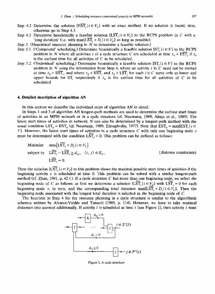
The heuristic in Step 4 for the resource planning in a cycle structure is similar to the algorithmic schemes written by Alvarez-Vald6s and Tamarit (1989, p. 114). However, we have to take maximal distances into account additionally. If activity l is scheduled at time t (see Figure 1), then activity i must

> ~ i ~ Sr(l)

dil < 0 (

dly> 0 V--q > [j~--->----j q~ er(i)

L__J

Figure 1. A cycle structure


be scheduled at the latest at time t + I dit l. We denote this upper bound of time with maxsti and the corresponding initiating activity 1 with predi = l.

Let .Jr be a set of activities which can be scheduled at time t. A conventional priority rule, for example SPT (shortest processing time), will assign an activity with the shortest duration the highest priority to be scheduled. A priority rule on A must be a reflexive, transitive and total binary relation on d (cf. Knuth, 1973, p. 3 f.). We now give the rule that enables us to apply conventrional priority rules to MPM projects.

maxst rule. Let i, j ~A', let O 6 be a conventional priority rule on .,¢', and let D(i) and D ( j ) be 'duration equivalent values' and of i and j. It holds that i ~ j Imaxst (i.e. i is prior to j concerning to the maxst rule) if one of the following conditions is satisfied:

(a) t + D( i ) > maxstj, t + D ( j ) > maxst i and maxsti < maxst r (b) t + D( i ) > maxstj, t + D ( j ) > maxsti, maxsti = maxstj and i ~<j 1 06 . (c) t + D(i) < maxstj and t + D ( j ) > maxsti. (d) t + D(i) < maxst/, t + D ( j ) < maxsti and i ~ j I O a. The inequality t + D( i ) > maxst~, means that the start of activity i at time t may prevent activity j from

being started up to its upper bound maxstj because of scarce resources. The maxst rule is an 'overriding' rule. In most cases the priorities of activities are assigned according to a conventional priority rule 0 6. Only if some upper bounds are 'at risk' (i.e. cases (a) and (c)), then the priorities of activities are assigned according to the corresponding urgencies with respect to their upper bounds.

Theorem 5. The maxst rule is a reflexive, transitive and total binary relation on ~ i f D(i ) = D ( j ) for all i, j ~At'.

Proof. Suppose D(i) = c for all i ~ .d . At a time t the set ~ can be divided into two sets:

J r " = {i ~ l t + c > maxsti} and Jr '" = {i ~g " I t + c < maxsti}.

From condition (c) in the maxst rule it follows that each activity in ~ ' has a higher priority than every activity in .,g". The priorities of activities in .,g" are determined only according to rule O 6 and the priorities of activities in .,¢" are determined according to rule O o or condition (a) which corresponds to a conventional priority rule with maxsti for all i ~ as the evaluating criterion. So the maxst rule is reflexive and total on ~ and transitive within the set .Jr ' or .,~'". We see that from i ~ j ~ k, i ~.,g," and k ~-..,¢'", it always follows that i ~ k, no matter whether j ~ .~" or j ~ ¢ ' " . So the maxst rule is transitive on ~ ' . []

According to the meaning of D(i) the constant c can be chosen between 0 and max{Dili ~-.,¢'}. Ideally, we have to chose D(i) as D i. But, unfortunately, the maxst rule in this case has been found to be non-transitive (cf. Zhan, 1991, p. 54 ff.).

The maxst rule assigns higher priorities to activities whose upper bounds are 'at risk' than to other activities. However, this rule does not give any guarantee that every activity will be scheduled by its upper bound. Hence, before scheduling an activity we have to examine whether the corresponding upper bound has been exceeded or not. If an upper bound is exceeded, we must stop scheduling activities and check why and at what time that happened. We consider now the following example.

Example 1. (See Figure 2.) First, node 1 is scheduled at time t---0; second, node 2 is scheduled at the same time (suppose node 2 has higher priority than node 4 through some priority rules) so that we have maxst 3 = 3 and pred 3 = 2. At time t = 1 node 4 is scheduled. Then we are faced with a conflict: according to maxst 3 = 3 node 3 must be scheduled no later than t = 3 but this is not possible because there are only 2 units of resource available. It is easy to see that node 4 must be scheduled earlier than node 2. However, if there is no arc (4, 3), but an arc (2, 4) with d24 = 1 instead, then node 4 must be scheduled later than node 3. If both cases cannot be distinguished correctly, e.g. when in the first case we

J. Zhan / Scheduling resource-constrained projects in MPM networks 199 < ~ ~<~3~15 ~ O 2>--3

I o

- 6 <

capacity R 1 = 5

Figure 2. legend:

try to schedule node 4 even later, then the planning will be caught in a end less loop. In general, even more complicated cases can occur. In this paper, the following backward-planning method is developed for the case that some upper bounds are exceeded.

The essential idea of the backward-planning method is as follows. A lower bound minsty is assigned to every activity j. Once it is detected than an activity i with pred i = 1 cannot be scheduled till time t > maxsti, there are some causes that account for preventing activity i from being scheduled till t (see the cycle structure in Figure 1): either activity l has been scheduled too early because a real generalized predecessor of i (e.g. node h) was scheduled later than ST t, or activity j which is no real generalized predecessor of i has been scheduled too early so that there is not enough resource capacity available for activity i to be scheduled till t ime t, or a combination of both account for it. Let AV be set of activities which are scheduled at a t ime no later than ST~ and they do not belong to any path with non-negative length from 1 to i. Then the backward-planning procedure can be described as follows: Step 1. If AV contains an activity j which is a real generalized successor of 1, set minstj to a later time

than the current STy, t o = STj and go to Step 5. Step 2. Otherwise, if AV contains an activity h which is a real generalized predecessor of i, set minst t to

a later t ime than the current STt, t o = ST~ and go to Step 5. Step 3. Otherwise, if AV contains an activity k which is a fictitious generalized successor of l, set minst k

to a later time than the current STk, t o = STg and go to Step 5. Step 4. Otherwise, if AV contains an activity which is a fictitious generalized predecessor of i, set minst t

to a later t ime than the current STt and t o = ST t. Step 5. Reconstruct the ' s ta te ' of scheduling at the time t o , i.e., reverse all the schedules which have

been done since t o and redetermine the upper bounds of all activities which have been obtained since t 0. Then, continue the scheduling process from time t 0. In the meant ime activity l, j or k will be prevented from being scheduled at t ime t o through the new enlarged lower bounds.

Using the maxst rule and the backwards-planning method exposed above, the algorithm for resource planning in a cycle structure can be stated as follows (cf. Alvarez, 1989, p. 114), where . ~ is the set of activities which have already been scheduled, and an activity i 'can ' be scheduled at time t if every activity in p r ( i ) has been scheduled and it holds that ST k + dki > t for all k ~ Pr(i) and t > minsti.

Algorithm AC. I~ t C = (V¢, E c ) be a cycle structure, {EST/I i ~ V c} and {LST/I i ~ V c} be solutions to t ime planning in

C and T = max{LSTi I i ~ Vc}. Step 1. (Initialization.) Set t = 0, . ~ = ~, ESTi = - 1, predi = 0, minsti = ESTi and maxsti = LST i for all

i vc. Step 2. (Construction of ~f.) Set ~tr = set of activities which can be scheduled at t ime t.

If ~tr = ¢ and 2 4: V c, then go to Step 5. If M = ¢ and .Z/= V c, stop (all activities have been scheduled).


Step 3.

Step 4.

Step 5.

(Priority rule.) Order .,¢ according to the maxst rule with chosen priority rule Oa. If some i ~.,¢ with maxsti < t exist, carry out the backward planning and go to Step 5. (Construction of the schedule.) Assign time t to the start time EST i of activities i ~ -~ one after another until there is not enough resource capacity available for scheduling any more activity in

.¢t" at time t. Insert activities that have been scheduled at time t in set _W. Update maxst i and pred i for all i ~ Vc\.Z~. (Determining a new time t.) Find the minimum among all E s T i + D i > t and EST i + d# > t with i ~ S ° and ( i , j ) ~ E c. Set the new time t to equal to the minimum. If t > T, stop (there is no feasible solution), otherwise go to Step 2.

If we apply algorithm AC to the cycle structure in Figure 2, then ESTg = 0, 3, 5, 0, 5, 7 for i = 1, 2 , . . . , 6, respectively, will be the feasible solution found. Undoubtedly, some calculational improve- ment can be made in algorithm AC because only the principle, not any exact calculating procedure is described by it. Algorithm AC does not guarantee to provide a feasible solution. If no feasible solution has been found, we can only use an exact method (cf. Patterson, 1984) for making sure whether a feasible solution does exist. If one exists, it is used as the solution to the RCPS problem in C.

In the following we will discuss the method developed for Step 4.3 of algorithm AN, where a feasible solution {EgT i l i ~ V c} is assumed to have already been determined in Steps 4.1 or 4.2 of algorithm AN. For finding the solution {LSTi [i ~ V c} with a ' longer duration' we make use of the available feasible solution {Eg-T/[i ~ V c} in the following way: At first we s e t ~ - - T i ~- ESTi for every i ~ V c. A n activity i is called 'pushable' if

LST----~ < min{~---Tj - dij I~'Tj ~ ~ - T i , i ~ . ~ ( j ) , dij < 0}.

Then, with all the distance and capacity constraints always being satisfied, we push (or enlarge) every ~----T i as far as possible. The method is based on the following theorem.

Theorem 6. Let {ST i l i e V c} be a feasible solution to the CPS problem in a cycle structure C with the beginning node s, let M 1 and M E be sets with M 1 U M E = V o M 1 A M 2 = O, s ~ M 1 and ST/> STj f o r all i ~ M 2 and j ~ M 1. I f there exists a A ~ ~ with ST i + A < STj - dij for all ( i , j ) ~ E o i ~ M 2 and j ~ M 1, then {ST/' I i ~ Vc}, with

ST/, i ~ M1,

ST/ '= S T / + A , i ~ m 2 ,

is a feasible solution to the R C P S problem in C.

Proof. For art arc (i , j ) ~ E c the following 4 cases have to be considered: 1) i, j ~M1; 2) i, j ~ME; 3) i ~ M 1 and j ~ M2; 4) i ~ M E and j ~ M 1. Obviously, the distance constraint STj' - ST/' ___ dij is satisfied for the first three cases. From

S T i --[- A ~ S T j - bij :=~ STit <~ S T f - bij ~ STj' - ST/' > bij

we see that the distance constraint for case 4) is also satisfied. To examine the capacity constraints, we denote t o = m a x { S T / I / ~ M 1} and see the capacity constrints are satisfied within the time period [0, t o + A]. For t > t o + a it holds that

{il t - O i < ST/' =< t} = {il t - O i < STi + A __< t and ST/> to} tA {il t - O i < STi _< to}.

From

{il t - D i < ST/+ A < t and ST/> to} = {il t - D i - A < ST i < t - A and ST/> to}

J. Z h a n / Scheduling resource-constrained projects in M P M networks 201

and

{i l t - O i < S T / < / 0 } --- { i l l - O i - A < S T / < t - A and S T / < to}

it follows that {i I t - D~ < ST/' < t} g {i I t - D~ - zi < ST~ < t - A} = V(t - A). From the feasibility of the solution {ST/I i ~ V c} it follows that the capacity constraints are satisfied for t > t o + A. []

Based on this t heo rem the ' push ing ' me thod can be cons t ruc ted as follows. At first the set V c is divided into sets M 1 and M z with M~ = {s}. T he value zl can be de te rmined f rom all pushable activities in M 2. If A > 1, the start times of all activities in M 2 are increased by zi, otherwise (i.e. zl < 1) the latest t ime ~- among all ST/ of every activity i ~ ME, which is not pushable and satisfies the condit ion S'~(i) • M~ :~ ~t, has to be determined. Then all activities j ~ M 2 with start t ime no later than ~- are to be put into set Ma. This p rocedure is to be repea ted until M 2 = ~t.

Example 2. Let ESTi = 0, 3, 5, 0, 5, 7 for i = 1, 2 . . . . . 6, respectively, be the feasible solution to the cycle s t ructure C illustrated in Figure 2 with beginning node 1. At first we have M 1 = {1}, M 2 = {2, 3 . . . . . 6} and LS-T~ = 0. Because (6, 1) is the only arc f rom M 2 to M 1, we have zl = 15 - 7 = 8. Then we have the solution {LS-Ti I i ~ C} = {0, 11, 13, 8, 13, 15}.

The advantage o f this me thod is that it can provide a feasible solution, for certain. We can still const ruct an alternative me thod which schedules activities backwards in a similar way as algori thm AC, but such a me thod cannot guaran tee a feasible solution.

Now we consider heuristics for resource planning in networks instead of cycle structures. The main idea of the heurist ic used in Step 5.1 of a lgori thm A N is that every activity i of a cycle s tructure C has the start t ime ST i = t o + ESTi if t o is the earliest t ime in N for every activity of C to be scheduled, where {ES-Ti I i ~ V c} is the solution de te rmined in Step 4.1 or 4.2 of AN. In some sense the activities of a cycle s tructure are scheduled toge ther as a single ' c o m p o u n d ' activity with variable resource demands at different t ime periods; e i ther no activity of the cycle s tructure is scheduled or every activity of the cycle s t ructure has been scheduled. To schedule a cycle structure means to schedule all activities of the cycle structure. If every beginning activity of C can be scheduled, then cycle s tructure C can be ~cheduled.

Dur ing heuristical resource planning with priority rules, priorities will be assigned to activities according to cor responding data, so we have to decide how the data that is d e m a n d e d by a priority rule are defined for cycle structures. These data can be s tructure based (e.g. IS(i)1), t ime based (e.g. EST/, LST i and maxsti), or dura t ion and resource based (e.g. D i and rik) , etc. Let s be the beginning node of cycle s tructure C. We use the same structure or t ime based data of node s for cycle s tructure C as follows:

S ( C ) = S(s) , EST c = ESTs, LST c --- LSTs, maxst c '.= maxst r The dura t ion and resource based data for a cycle s tructure C is given by

D c = m a x { E - S T i + D i l i ~ V c } and rCk= ( ~ _ ~ r i k ' D i ) \ D c f o r k = l . . . . ,q . i ~ C

With such data for cycle s tructures the resource planning in a network N can be carr ied out heuristically in the same way as for a lgori thm AC. The modificat ions needed in algori thm A C are to replace a cycle s t ructure in N by a c o m p o u n d activity. Because activities of a cycle s tructure are scheduled in the same way as shown in the p roof of T h e o r e m 4, a feasible solution to the RCPS problem in N will be certainly obta ined at its terminat ion. Now we give an example to show the comput ing p rocedure of Step 5.1 of AN.

Example 3. We consider the ne twork N shown in Figure 2, but wi thout arc (6, 1). N contains two cycle structures, C x (with nodes 2 and 3) and C 2 (with nodes 4 and 5). By Step 4 of A N we get solution EST 2 = 0, ES--T 3 = 2 for C 1 a n d ES-T 4 = 0, E S T 5 = 3 for C 2. At time t = 0 both C 1 and C 2 can be


scheduled. I f C 2 has a higher priority than C 1, then C 2 is scheduled at t = 0 with ST 4 = 0, ST 5 = 3, C 1 a t

time t = 5 with ST 2 = 5, ST 3 = 7 and node 6 with ST 6 = 9 (project duration). On the other hand, if C2 has a lower priority than C1, then C 1 is scheduled at t = 0 with ST 2 = 0, ST 3 = 2 so that we have maxstc2 = 2 and predc2 = C r We see then, because C 2 cannot be scheduled till t = 2 and C 2 is a real predecessor of C1, C1 must be scheduled later than C 2. After reconstructing the 's tate ' of scheduling at t ime 0, scheduling can be continued and the same result (ST 6 = 9) will be achieved finally.

In Step 5.2 of algorithm AN, activities of a cycle structure C are scheduled individually, i.e., we need not have ST/= to + ESTi for every i ~ V c if t o is the earliest t ime in N for all i ~ V c to be scheduled. The solutions {ES-Ti I i ~ V c} and {LS--Ti I i ~ l/c} serve only to determine the lower and upper bounds minsti and maxsti for every i ~ V c so that minst i > t o + EST i and maxsti < t o + ~ - - T i hold. However, some heuristics for cycle structures are required to maintain the feasibility of the solution as far as possible.

Suppose a network N contains two cycle structures, C ' and C", suppose an activity i ~ C ' is a real generalized predecessor of an activity j ~ C" with positive length, and the corresponding path from activities i to j has no common arc with C ' and C". We call C ' a 'pre-cycle structure of C ' and activity i a 'predecessor ' of a 'pre-cycle structure of C'. In example 2, C 2 is a pre-cycle structure of C 1 with corresponding predecessor node 4. I f there is not enough resource capacity available to schedule activities of both cycle structures, activities in C ' have to be scheduled first instead of activities in C". I f activity i has already been scheduled, possible start times of activities in C" are independent from C ' so that we can try to schedule activities in C" immediately. The heuristic for cycle structures is that an activity of cycle structure C" can only be scheduled if predecessors of every pre-cycle structures of C are all scheduled already. In other words, this heuristic assigns priorities to cycle structures with respect to the structure of the network so that cycle structures will be scheduled one after another in some ' topological order ' . With this heuristic we can use Algorithm AC with corresponding extension for Step 5.2 of algorithm AN.

Sometimes the heuristic for Step 5.2 of AN provides bet ter solutions than the heuristic for Step 5.1 of AN because during individual planning more possibilities are examined. But the heuristic for Step 5.2 does not guarantee a feasible solution even if one exists. Let us sonsider the following example.

Example 4. We apply Step 5.2 of algorithm AN to the same network in Example 3. At time t = 0 only node 4 can be scheduled because C 2 is a pre-cycle structure of C r At t = 3 node 2 is scheduled because maxst 5 = 6 is not 'at risk' yet. Then node 5 is scheduled at t = 4 and node 6 at t = 7. We see the corresponding project duration is 7 t ime units which is shorter than 9 in Example 3.

5. Computational results

In this section we give some computat ional results for evaluating the performance of heuristics developed in this paper, where different priority rules are used. All the heuristics and priority rules were implemented in C on a HP9000/360 computer . More than 800 test problems were generated by a network generator for MPM networks, which had been developed in our institute. Some characteristics of MPM networks are quite different from that of CPM networks, so we give some important characteristics used for randomly generating networks below, where the values of characteristics used are given in brackets: 1. n: number of activities (20, 30, 40, 50, 100, 300, 1000). 2. q: number of resources (1, 3). 3. re~n: density (1.5, 2.5) (e.g. the example from Bartusch et al., 1988, has density 2). 4. ( - 3 - a)/oz: cycle elasticity, where a denotes the sum of positive arc weights and fl the sum of

negative arc weights of a cycle C. The mean values of cycle elasticity used are 0.5 and 1.

J. Zhan / Scheduling resource-constrained projects in MPM networks

Table 1 Comparison between best solutions from heuristics and optimal solutions

203

Number of activities 20 30 40 50

Number of problems with optimal solution 71 53 57 52

Number of problems solved by heuristics with opt imum 39 23 18 10

- in percent (%) 54 43 32 19 Average deviation (%) 2.38 1.79 1.80 1.64 Standard deviation ~r (%) 4.91 2.31 1.91 1.74 0.95-Quantile a (%) 13.58 6.96 6.98 6.25

a For 95% all test problems the deviation is smaller than the 0.95-quantile.

5. Number of cycle structure (2, 3, 4, 5, 8, 12 and 20 for n = 20, 30, 40, 50, 100, 300 and 1000 respectively).

6. Maximal size of cycle structures (7). 7. Distribution of values of activities and distances:

D i ~ [0, 16] belongs to a truncated normal distribution with expected value E(D i) = 8 and standard deviation or = 4. rik ~ [0, 9] equally distributed, R k = 12. The percentage of activities which demand resource 1 is 95%, that for resource 2 is 50% and that for resource 3 is 50%, too. dii ~ [0, 20] equally distributed, where it holds that dii = D i for 70% of all distances and dii > Di for 20% of all distances. The test problems can be divided into three groups: problems of small size (20, 30, 40 and 50

activities) with 1 resource, problems of large size (100, 300 and 1000 activities) with 1 resource and problems with 3 resources. The problems of small size were used to access the performance of suboptimal solutions obtained by heuristics because both the exact method and heuristics can be applied to them. The problems of large size serve to investigate the behavior of heuristics with different sizes of problems. The last group was used to test the behavior of heuristics with multi-resources. To each test problem algorithm AN was applied respectively with each of the 27 priority rules used. Twenty-four of these rules come from Alvarez-Vald6s and Tamarit (1989, except rules MJP and GRU) and the other

q three rules are R U R (Resource Utilization Ratio, max Ek=~rik/Rk), WRUP (Weighted Resource Utilization and Precedence, cf. Ulusoy and Ozdamar, 1989) and POPb (Product of Priorities from rules LFS, LST, MTS and LPF).

Table 1 gives the results for the first group of test problems. To each problem the shortest project duration from 27 solutions is used for the comparison with the corresponding optimum obtained by the exact Bartusch method (1983). The reason is that we only want to know the performance of heuristics in comparison with optimal solutions, along with increasing size of problems. Suppose for a certain problem j the shortest project duration with heuristics is hj and the optimum is Oi, then the deviation (h i - O j ) / O i represents the relative performance of the underlying heuristic.

The results in Table 1 allow the conclusion that the size of the test problem is an important factor for the performance of heuristics. Along with the increasing size of the test problems the average deviation, the standard deviation o- and the 0.95-quantile of the deviation become even smaller. This tells us that particularly for problems of large size we have more reason to use heuristics than exact methods. Even for problems of small size we cannot expect to obtain optimal solutions within a given realistic time limit by using exact methods; e.g. for test problems with 20 activities some of the optimal solutions were achieved within 5 minutes (user time) while another one needed more than 80 hours. The average deviation of the best suboptimal solutions for projects of small size are not large at all (e.g. 1.80% and 1.64% for projects with 40 and 50 activities). So we can say that conventional priority rules developed for CPM networks can be successfully applied to MPM networks by using the heuristics in this paper.

204

Table 2 Average deviation in percent a

J. Zhan / Scheduling resource-constrained projects in MPM networks

Number of activities 50 100 300 1000

Best rule combination 1.15 0.33 0.05 0.07 LPT 1.57 1.00 0.73 0.45 RSM 1.63 1.02 0.80 0.34 MTS 2.10 2.10 1.81 1.19 MIS 3.27 4.12 6.76 7.22 R A N D O M 2.97 4.32 8.18 8.52 LTS 5.06 7.95 13.90 14.41

a 80 test problems were used for each number of activities.

Table 3 Average computing time (sec) of heuristics

Number of activities

20 30 40 50 100 300 1000

1 resource 0.157 0.266 0.51 0.742 2.552 11.657 20.802 3 resources - 0.49 - 1.227 4.349 25.49 -

Table 2 gives the average deviation of solutions by heuristics with respect to the best known solution of the heuristics with one of the 27 priority rules. In Table 2 the term 'rule combination', which is also investigated by Boctor (1990), means to use more than one heuristic and to retain the best of the solutions obtained. A rule combination in our test consists of 4 different priority rules. The results in Table 2 can be summarized as follows: 1. The results tend to support previous findings (cf. Alvarez-Vald6s and Tamarit, 1989; Boctor, 1990):

Priority rules that are most effective in CPM networks, such as LFT, RSM, LST, etc., are also most effective in MPM networks.

2. The size of the test problems scarcely affects the relative rank of performance of the priority rules. The most effective priority rules for small problems are also the most effective for large problems (cf. Alvarez-Vald6s and Tamarit, 1989, p. 121; Boctor, 1990).

3. Along with increasing size of the test problems the distinctions between different priority rules become more statistically significant, i.e., good rules such as LFT and RSM become even better and bad rules such as LTS become even worse.

4. None of the heuristic rules performed consistently best on all problems. But in a statistical sense the best rule combination performed always bet ter than any single rule. Best rule combinations consist of the rules RSM, LST, R A N D O M and MINS for n = 20, LFT, RSM, LNRJ and GPRP for n = 50, LST, RSM, POPb and LPF for n = 100, LFT, RSM, LST and MTS for n = 300, and LFT, RSM, LST and R UR for n = 1000 respectively. Table 3 shows the average computing times of heuristics for different number of activities and

resources. We see the average computing times of heuristics grow nearly linear with increasing number of activities. So we can use the best rule combination even for large problems. The 4 conclusions drawn from Table 2 hold for the third group, too. It was also found that the number of resources scarcely affects the relative rank of performance of the priority rules.

References

Ahuja, R.K., Magnanti , T.L., and Odin, J.B., (1989), "Network flows", in: G.L. Nemhause r et al. (eds.), Handbooks in OR & Management Science, Elsevier, Amste rdam, 258-263.


Alvarez-Vald6s, R., and Tamarit, J.M. (1989), "Heuristic algorithms for resource-constrained project scheduling: A review and an empirical analysis", in: R. Stowifiski and J. W~glarz (eds.), Advances in Project Scheduling, Elsevier, Amsterdam, 113-134.

Balas, E. (1971), "Project scheduling with resource constraints", in: E.M.L. Beale (ed.), Applications of Mathematical Programming Techniques, English University Press, London, 187-200.

Bartusch, M. (1983), "Optimierung von NetzplS.nen mit Anordnungsbeziehungen bei knappen Betriebsmitteln", Ph.D. Disserta- tion, Aachen University, Germany.

Bartusch, M., M6hring, R.H., and Radermacher, F.J. (1988), "Scheduling project networks with resource constraints and time windows", :A'.hnals of Operations Research 16, 201-240.

Battersby, A. (1977), Network Analysis for Planning and Scheduling, Macmillan, London, 91 ft. Boctor, F.F. (1990), "Some efficient multi-heuristic procedures for resource-constrained project scheduling", European Journal of

Operational Research 49, 3-13. Cooper, D.F. (1976), "Heuristics for scheduling resource-constrained projects: An experimental investigation", Management

Science 22/11, 1186-1194. Davis, E.W., and Heidorn, G.E. (1971), "Optimal project scheduling under multiple resource constraints", Management Science

17/12, 803-816. Davis, E.W., and Patterson, J.H. (1975), "A comparison of heuristic and optimum solutions in resource-constrained project

scheduling", Management Science 21/8, 944-955. Elmaghraby, D.E. (1977), Activity Networks: Project Planning and Control Network Models, Wiley, New York. Even, S. (1979), Graph Algorithms, Pitman, London, 64 ft. Garey, M.R., and Johnson, D.S. (1979), Computers and Intractability: A Guide to the Theory of NP-Completeness, Freeman, San

Francisco, CA. Knuth, D.E. (1973), The Art of Computer Programming, Addison-Wesley, Reading, MA. Lawler, L.E. (1979), Combinatorial Optimization: Networks and Matroids, Holt, Rinehart & Winston, New York. Neumann, K. (1989), "Netzplantechnik", in: T. Gal (ed.), Grundlagen des Operations Research Vol. 2, Springer, Berlin. Patterson, J.H. (1984), "A comparison of exact approaches for solving the multiple constrained resource project scheduling

problem", Management Science 30/7, 854-867. Roy, B. (1959), C.R. Acad. Sciences, T. 248, 2437. Ulusoy, G., and Ozdamar, L. (1989), "Heuristic performance and network/resource characteristics in resource-constrained project

scheduling", Journal of the Operational Research Society 40/12, 1145-1152. Zhan, J. (1991), "Heuristische Ressourcenplanung in MPM-Netzpl~inen mit beschr~inkter Kapazit~it", Ph.D. Dissertation, Karls-

ruhe University, Germany.

heuristics for scheduling resource-constrained projects in mpm networks

Documents