heft 175 sachin ramesh patil regionalization of an event
TRANSCRIPT

Heft 175 Sachin Ramesh Patil
Regionalization of an Event Based Nash Cascade Model for Flood Predictions in Ungauged Basins

Regionalization of an Event Based Nash Cascade Model for Flood Predictions in Ungauged Basins
Von der Fakultät Bau- und Umweltingenieurwissenschaften der Universität Stuttgart zur Erlangung der Würde eines Doktor-Ingenieurs (Dr.-Ing.) genehmigte Abhandlung
Vorgelegt von Sachin Ramesh Patil
aus Jalgaon, Indien
Hauptberichter: Prof. Dr. rer.nat. Dr.-Ing. habil. András Bárdossy Mitberichter: Prof. Dr.-Ing. Uwe Haberlandt
Tag der mündlichen Prüfung: 15. Juli 2008
Institut für Wasserbau der Universität Stuttgart 2008


Heft 175 Regionalization of an Event Based Nash Cascade Model for Flood Predictions in Ungauged Basins
von Dr.-Ing. Sachin Ramesh Patil
Eigenverlag des Instituts für Wasserbau der Universität Stuttgart

D93 Regionalization of an Event Based Nash Cascade Model for Flood Predictions in Ungauged Basins
Titelaufnahme der Deutschen Bibliothek
Patil, Sachin Ramesh: (Regionalization of an Event Based Nash Cascade Model for Flood Predictions in
Ungauged Basins / von Sachin Patil. Institut für Wasserbau, Universität Stuttgart. - Stuttgart: Inst. für Wasserbau, 2008
(Mitteilungen / Institut für Wasserbau, Universität Stuttgart: H. 175) Zugl.: Stuttgart, Univ., Diss., 2008) ISBN 3-933761-79-8 NE: Institut für Wasserbau <Stuttgart>: Mitteilungen
Gegen Vervielfältigung und Übersetzung bestehen keine Einwände, es wird lediglich um Quellenangabe gebeten. Herausgegeben 2008 vom Eigenverlag des Instituts für Wasserbau Druck: Document Center S. Kästl, Ostfildern

Acknowledgment
This research work was carried out under the supervision of Prof. Andras Bardossy.I feel greatly honored for being one of his students, his prodigious expertise hasunfailingly enlightened my path on this journey in the challenging territory of hy-drology and statistics. I would like to express my deep gratitude to him for providingme this wonderful opportunity to work with him. I greatly appreciate his enthusi-asm, guidance, and the many discussions and the critics which he shared with methroughout this work. Above all, I will cherish his ever optimistic attitude, whichnot only helped during this work but will be an asset for future too. I would also liketo express sincere thanks to Prof. Uwe Haberlandt for accepting to co-supervise thisresearch work and and for his valuable suggestions. Here I must also take the oppor-tunity to express my deepest gratitude to Prof. Helmut Kobus and Prof. BernhardWestrich for their indirect support and motivation.
I sincerely acknowledge ENWAT International Doctoral Program of UniversitaetStuttgart for providing the academic framework for this research work. I am greatlythankful to the financial support provided by IPSWaT Scholarship Program of Ger-man Federal Ministry of Education and Research (BMBF).
I would like to extend my acknowledgments further to Dr.-Ing. Jurgen Brommundtand Dr. rer.nat. Johannes Riegger for helping me to acquire the hydrological datawithout which this work would be impossible realize. Many many hearty thanks toPawan Kumar Thapa, Shailesh Singh, Dr.-Ing. Jens Gotzinger, Dr.-Ing. Tapash Dasand Dr.-Ing. Yi He for their cooperation and the troubleshooting they offered fromtime to time. I am grateful to Jeff Tuhtan and Ferdinand Beck for taking the pain tomake language corrections in the dissertation. I must mention Mrs. Krista Uhrmannfor her assistance in the bureaucratic matters and for patiently informing about theavailability of Prof. Bardossy every now and then. I cannot end this paragraphwithout mentioning Dr.-Ing Arne Farber for the orientation and care he providedduring the early days at the institute. Last but not least, I am thankful to all thoseunmentioned colleagues at the institute who have contributed to this work directlyor indirectly.
Throughout this work, my wife Jackelyn has been a great inspiration for me, withouther presence in my life I would not even have begun this endeavor. I would liketo mention my loving appreciation to her for the love, care and support she hascontinuously bestowed upon me. Although there are no words to express my feelingfor them, I would like to mention my deepest gratitude to my parents, my sisters,my brothers- and parents-in-law for their love and encouragement. Finally, I amthankful to God for granting me the resources and the strength to accomplish thisresearch work.
v

vi

Contents
List of Figures ix
List of Tables xi
Abstract xiii
Kurzfassung xviii
1 Introduction 1
1.1 Dealing with floods . . . . . . . . . . . . . . . . . . . . . . . . . . . . . 1
1.2 Design floods and their prediction . . . . . . . . . . . . . . . . . . . . 21.2.1 Historical flood records based methods . . . . . . . . . . . . . . 2
1.2.2 Runoff based methods . . . . . . . . . . . . . . . . . . . . . . . 3
1.2.3 Rainfall based methods . . . . . . . . . . . . . . . . . . . . . . 41.3 Rainfall-runoff modeling . . . . . . . . . . . . . . . . . . . . . . . . . . 5
1.3.1 Classification of rainfall-runoff models . . . . . . . . . . . . . . 51.3.2 Temporal scale of rainfall-runoff models . . . . . . . . . . . . . 6
1.3.3 Limitations of rainfall-runoff models . . . . . . . . . . . . . . . 81.3.4 Model parameters and calibration . . . . . . . . . . . . . . . . 8
1.4 Problem of predictions in ungauged catchments . . . . . . . . . . . . . 91.5 Objective of the study . . . . . . . . . . . . . . . . . . . . . . . . . . . 10
2 Regionalization of Hydrological Models and the Proposed Methodology 12
2.1 Regionalization: a state of art . . . . . . . . . . . . . . . . . . . . . . . 122.1.1 Direct parameter transfer approach . . . . . . . . . . . . . . . . 12
2.1.2 Regional transfer function approach . . . . . . . . . . . . . . . 142.2 Existing methods for flood predictions in ungauged catchments . . . . 17
2.2.1 SCS method . . . . . . . . . . . . . . . . . . . . . . . . . . . . 17
2.2.2 Lutz procedure . . . . . . . . . . . . . . . . . . . . . . . . . . . 192.3 The proposed methodology . . . . . . . . . . . . . . . . . . . . . . . . 22
2.3.1 The rainfall-runoff model . . . . . . . . . . . . . . . . . . . . . 222.3.2 Flood routing . . . . . . . . . . . . . . . . . . . . . . . . . . . . 27
2.3.3 Regionalization of the model parameters . . . . . . . . . . . . . 28
3 Overview of the Study Area and the Hydrological Characteristics 30
3.1 General description of the study area . . . . . . . . . . . . . . . . . . . 30
3.2 Data situation of the study area . . . . . . . . . . . . . . . . . . . . . 313.3 Selection of catchments and events . . . . . . . . . . . . . . . . . . . . 31
3.3.1 Estimation of rainfall . . . . . . . . . . . . . . . . . . . . . . . 333.4 Estimations of hydrological characteristics . . . . . . . . . . . . . . . . 36
vii

3.4.1 Event specific characteristics . . . . . . . . . . . . . . . . . . . 373.4.2 Catchment specific characteristics . . . . . . . . . . . . . . . . 38
4 Regionalization of Rainfall Loss 45
4.1 Runoff coefficient . . . . . . . . . . . . . . . . . . . . . . . . . . . . . . 454.2 Transfer function for rainfall loss . . . . . . . . . . . . . . . . . . . . . 46
4.2.1 Multiple Linear Regression . . . . . . . . . . . . . . . . . . . . 484.2.2 Artificial Neural Network . . . . . . . . . . . . . . . . . . . . . 494.2.3 Fuzzy Logic . . . . . . . . . . . . . . . . . . . . . . . . . . . . . 524.2.4 Logistic Regression . . . . . . . . . . . . . . . . . . . . . . . . . 56
4.3 Validation for physical relationships . . . . . . . . . . . . . . . . . . . 614.3.1 Derivatives of physical relationships . . . . . . . . . . . . . . . 614.3.2 Derivatives of functional relationships . . . . . . . . . . . . . . 624.3.3 Comparison of the derivatives . . . . . . . . . . . . . . . . . . . 62
4.4 Comparison of LoTF with existing practices . . . . . . . . . . . . . . . 664.4.1 Modified SCS curve number method . . . . . . . . . . . . . . . 664.4.2 Lutz procedure . . . . . . . . . . . . . . . . . . . . . . . . . . . 68
4.5 Discussion on the estimation error of LoTF . . . . . . . . . . . . . . . 68
5 Regionalization of Nash Cascade Parameters 71
5.1 Nash cascade parameters . . . . . . . . . . . . . . . . . . . . . . . . . 715.2 Transfer functions for Nash cascade parameters . . . . . . . . . . . . . 71
5.2.1 Inter-parameter relationship . . . . . . . . . . . . . . . . . . . . 735.2.2 Selection of the predictors . . . . . . . . . . . . . . . . . . . . . 755.2.3 Form of the transfer functions . . . . . . . . . . . . . . . . . . . 765.2.4 Regional optimization procedure . . . . . . . . . . . . . . . . . 795.2.5 Simulated annealing algorithm . . . . . . . . . . . . . . . . . . 805.2.6 The optimization results . . . . . . . . . . . . . . . . . . . . . . 815.2.7 The validation results . . . . . . . . . . . . . . . . . . . . . . . 845.2.8 Comparison with the preliminary performance . . . . . . . . . 86
5.3 Validation for physical relationships . . . . . . . . . . . . . . . . . . . 875.4 Comparison with Lutz procedure . . . . . . . . . . . . . . . . . . . . . 885.5 Discussion on the estimation error . . . . . . . . . . . . . . . . . . . . 91
6 Case Study: Catchment Tubingen 93
6.1 Application of the regionalization methodology . . . . . . . . . . . . . 936.1.1 Description of the case study . . . . . . . . . . . . . . . . . . . 936.1.2 Estimation of runoff coefficient . . . . . . . . . . . . . . . . . . 936.1.3 Estimation of Nash cascade parameters . . . . . . . . . . . . . 966.1.4 Estimation of flood hydrograph . . . . . . . . . . . . . . . . . . 97
6.2 Assessment of impact of land use changes . . . . . . . . . . . . . . . . 98
7 Summary and Outlook 102
7.1 Summary . . . . . . . . . . . . . . . . . . . . . . . . . . . . . . . . . . 1027.2 Outlook . . . . . . . . . . . . . . . . . . . . . . . . . . . . . . . . . . . 106
References 107

List of Figures
1.1 Calibration procedure for rainfall-runoff models . . . . . . . . . . . . . 9
2.1 Derivation and application of regional transfer function . . . . . . . . 15
2.2 SCS dimensionless and triangular unit hydrograph . . . . . . . . . . . 19
2.3 Unit hydrograph of 1 hour duration . . . . . . . . . . . . . . . . . . . 23
2.4 Superposition of direct runoff hydrographs . . . . . . . . . . . . . . . . 23
2.5 Concept of Nash cascade linear reservoirs . . . . . . . . . . . . . . . . 25
2.6 Semi-distributed, event based Nash cascade model . . . . . . . . . . . 26
3.1 Overview of the study area and selected catchments . . . . . . . . . . 32
3.2 Maximum spec. peak runoff . . . . . . . . . . . . . . . . . . . . . . . . 35
3.3 Mean spec. peak runoff . . . . . . . . . . . . . . . . . . . . . . . . . . 35
3.4 Maximum total rainfall . . . . . . . . . . . . . . . . . . . . . . . . . . 35
3.5 Mean total rainfall . . . . . . . . . . . . . . . . . . . . . . . . . . . . . 35
3.6 Interpolated hourly rainfall and corrected hourly rainfall . . . . . . . . 36
3.7 Mean slope . . . . . . . . . . . . . . . . . . . . . . . . . . . . . . . . . 41
3.8 Mean top. wetness index . . . . . . . . . . . . . . . . . . . . . . . . . . 41
3.9 Mean top. ruggedness index . . . . . . . . . . . . . . . . . . . . . . . . 41
3.10 Mean river density . . . . . . . . . . . . . . . . . . . . . . . . . . . . . 41
3.11 Soil classes . . . . . . . . . . . . . . . . . . . . . . . . . . . . . . . . . 43
3.12 Mean field capacity . . . . . . . . . . . . . . . . . . . . . . . . . . . . . 43
3.13 Land use in year 1993 . . . . . . . . . . . . . . . . . . . . . . . . . . . 43
3.14 Land use in year 2000 . . . . . . . . . . . . . . . . . . . . . . . . . . . 43
4.1 Runoff coefficient method . . . . . . . . . . . . . . . . . . . . . . . . . 46
4.2 Constant loss rate method . . . . . . . . . . . . . . . . . . . . . . . . . 46
4.3 Straight line hydrograph separation method . . . . . . . . . . . . . . . 47
4.4 Performance of MLTF over regionalization set . . . . . . . . . . . . . . 50
4.5 Performance of MLTF over validation set . . . . . . . . . . . . . . . . 50
4.6 An artificial neuron . . . . . . . . . . . . . . . . . . . . . . . . . . . . . 51
4.7 Artificial Neural Network . . . . . . . . . . . . . . . . . . . . . . . . . 51
4.8 Performance of ANNTF over regionalization set . . . . . . . . . . . . . 53
4.9 Performance of ANNTF over validation set . . . . . . . . . . . . . . . 53
4.10 Performance of FLTF over regionalization set . . . . . . . . . . . . . . 55
4.11 Performance of FLTF over validation set . . . . . . . . . . . . . . . . . 55
4.12 Logistic Relationship . . . . . . . . . . . . . . . . . . . . . . . . . . . . 56
4.13 Physically unreasonable functional relationship between PlC and Tp . 59
4.14 Performance of LoTF over regionalization set . . . . . . . . . . . . . . 60
4.15 Performance of LoTF over validation set . . . . . . . . . . . . . . . . . 60
ix

4.16 Functional relationships between PlC and the predictors; A. Pt, B .API, C . DR, D . FCm, E . M , F . LUf/LUu. . . . . . . . . . . . . . . 63
4.17 Performance of SCS curve number method over validation set . . . . . 674.18 Validation performance of Lutz procedure . . . . . . . . . . . . . . . . 674.19 PlC vs. relative error . . . . . . . . . . . . . . . . . . . . . . . . . . . 694.20 Pt vs. relative error . . . . . . . . . . . . . . . . . . . . . . . . . . . . . 694.21 Spatial distribution of mean relative error for catchments . . . . . . . 69
5.1 Distribution of Nash cascade parameters corresponding to high good-ness fit performance . . . . . . . . . . . . . . . . . . . . . . . . . . . . 72
5.2 Inter-parameter relationship between N and K . . . . . . . . . . . . . 745.3 Trend line analysis of relationship between K and the potential pre-
dictors . . . . . . . . . . . . . . . . . . . . . . . . . . . . . . . . . . . . 775.4 Trend line analysis of relationship between β and the potential predictors 785.5 Regional optimization procedure . . . . . . . . . . . . . . . . . . . . . 805.6 Modeled runoff hydrograph for event: 15-281098 in catchment Oppen-
weiler . . . . . . . . . . . . . . . . . . . . . . . . . . . . . . . . . . . . 835.7 Modeled runoff hydrograph for event: 3-150601 in catchment Un-
termunstertal . . . . . . . . . . . . . . . . . . . . . . . . . . . . . . . . 835.8 Goodness fit: peak runoff . . . . . . . . . . . . . . . . . . . . . . . . . 845.9 Goodness fit: time to peak runoff . . . . . . . . . . . . . . . . . . . . . 845.10 Modeled runoff hydrograph for event: 27-241098 in catchment St.
Blasien . . . . . . . . . . . . . . . . . . . . . . . . . . . . . . . . . . . . 855.11 Modeled runoff hydrograph for event: 33-101097 in catchment Ettlingen 855.12 Goodness fit peak runoff . . . . . . . . . . . . . . . . . . . . . . . . . . 865.13 Goodness fit time to peak runoff . . . . . . . . . . . . . . . . . . . . . 865.14 Time of concentration (TC) versus unit hydrograph . . . . . . . . . . 895.15 Perimeter (Per) versus unit hydrograph . . . . . . . . . . . . . . . . . 895.16 Slope (SL) versus unit hydrograph . . . . . . . . . . . . . . . . . . . . 905.17 Urban land use (LUu) versus unit hydrograph . . . . . . . . . . . . . . 905.18 Goodness fit: peak runoff (Lutz procedure) . . . . . . . . . . . . . . . 915.19 Goodness fit: time to peak runoff (Lutz procedure) . . . . . . . . . . . 915.20 Total rainfall vs. NS . . . . . . . . . . . . . . . . . . . . . . . . . . . . 925.21 Duration vs. NS . . . . . . . . . . . . . . . . . . . . . . . . . . . . . . 925.22 Mean NS for the catchments . . . . . . . . . . . . . . . . . . . . . . . 92
6.1 Normalized temporal distribution of design storm rainfall (DVWK,1999) . . . . . . . . . . . . . . . . . . . . . . . . . . . . . . . . . . . . . 94
6.2 Rainfall time series . . . . . . . . . . . . . . . . . . . . . . . . . . . . . 946.3 Design flood hydrographs for different rainfall durations (Tubingen) . 986.4 Flood runoff hydrographs corresponding to the land use scenarios . . . 100

List of Tables
2.1 Curve number classification based on antecedent rainfall and seasons(SCS, 1972) . . . . . . . . . . . . . . . . . . . . . . . . . . . . . . . . . 18
3.1 Description of the available data . . . . . . . . . . . . . . . . . . . . . 333.2 Summary of the selected Catchments . . . . . . . . . . . . . . . . . . . 343.3 Soil classes based on hydraulic conductivity . . . . . . . . . . . . . . . 423.4 Statistics of the hydrological characteristics (HCs) . . . . . . . . . . . 44
4.1 Signs of derivatives of the physical relationships PlC and the predictors 624.2 Number of positive (+ve) and negative (-ve) changes in PlC corre-
sponding to the changes in the predictors for 211 events; A. LoTF,B . MLTF, C . ANNTF, D . FLTF . . . . . . . . . . . . . . . . . . . . 65
4.3 Statistics of absolute relative estimation error (%) . . . . . . . . . . . 68
5.1 Correlations of the hydrological characteristics with K, β and α . . . . 765.2 Aggregated performance of the derived transfer functions . . . . . . . 825.3 Aggregated preliminary performance (Monte-Carlo simulations) . . . . 865.4 Aggregated performance of Lutz procedure . . . . . . . . . . . . . . . 88
6.1 Hydrological characteristics of the subcatchments (Tubingen) . . . . . 956.2 Effective rainfall time series for the subcatchments (Tubingen) . . . . 976.3 Land use scenarios for the subcatchments (Tubingen) . . . . . . . . . 996.4 Design flood characteristics corresponding to the land use scenarios . . 1006.5 Ordinates of unit hydrograph and direct runoff hydrograph for the
subcatchments (Tubingen) . . . . . . . . . . . . . . . . . . . . . . . . . 101
xi

xii

Abstract
This study was aimed at developing a practical, robust and physically reasonablemethodology for estimation of design flood and its key characteristics under datascarce conditions. The key inputs for the planning and design of flood protec-tion schemes are the design flood characteristics, such as flood runoff volume, peakrunoff and time to peak runoff. The design flood characteristics are usually obtainedthrough discharge-frequency analysis or a hydrological model calibrated for the loca-tion under consideration. These approaches are based on two implicit assumptions:that a sufficient length of discharge time series is available, and the past of thecatchment represents its future. However, due to lack of sufficient discharge dataand inconstant hydrological conditions, application of discharge-frequency analysisor calibration of a hydrological model is not always viable. In such case, insteadof calibration, model parameters are obtained through regionalization procedure.The regionalization procedures usually associate model parameters with hydrologi-cal characteristics through regional transfer functions. A regional transfer functionfor a model parameter, derived using gauged catchments in a region, can be thenused to estimate the parameter for a “similar” ungauged catchment in the region,using its hydrological characteristics.
Most of the existing regionalization procedures derive a transfer function using twostep regionalization procedure: calibration of a model parameter for each of thegauged catchments separately, then establish the relationship between the calibratedparameter and hydrological characteristics through regression procedure. However,due to inter-parameter interaction, calibration often leads to more than one equallygood parameters (equifinality), thus not each of them may fit into a unique transferfunction. The derivation of a transfer function through the two step regionalizationprocedure, is subjected to parameter identification problem. The parameter identi-fication problem often leads to weak regional transfer functions. Besides, parametersets calibrated at catchment scale often do not correspond to an optimum parameterset at regional scales. To obtain an efficient and robust regionalization methodology,it must be developed for optimum regional performance instead of catchment specificperformance.
Furthermore, transfer functions are usually derived through purely-data-driven re-gression approaches. In doing so, the physical implications of the derived relation-ships, with respect to underlying rainfall-runoff processes, are usually disregarded.The purely-data-driven approach may lead to excellent goodness fit performance dur-ing regression, however the derived transfer function may not represent the physicalrelationships. Such transfer functions, due to their lack of a physical basis, can leadto erroneous and implausible predictions.
xiii

Abstract
The main objective of this study was to derive a regionalization methodology forflood predictions in ungauged catchments, which is strictly based on physically rea-sonable transfer functions, corresponding to the optimum regional performance andadequately addressing the problem of parameter equifinality. Not only catchmentspecific, but event specific hydrological characteristics were also considered duringthe study. Furthermore, a part of the study was intended to outline the significanceof physically reasonable approach for hydrological predictions. A possibility of as-sessment of impact of land use changes on flood characteristics was also investigatedduring the study.
An event based hourly Nash cascade model was developed to derive the directrunoff hydrograph from rainfall time series. The model was implemented on a semi-distributed scale, i.e. the direct runoff hydrograph is estimated at sub-catchmentscale (50 km2 to 75 km2), then it is routed to the outlet of the catchment using theMuskingum routing procedure. The model uses three model parameters, the runoffcoefficient (RC), the number of reservoirs (N) and a reservoir constant (K). For un-gauged catchments, the model parameters RC, N and K must be estimated througha regionalization procedure. The routing procedure uses two parameters: Musk-ingum retention constant (km) and weighting factor (xm), which were estimatedthrough a readily available empirical method. The study was focused on derivationof transfer functions to facilitate estimations of the model parameters RC, N and Kin ungauged catchments.
The study was conducted using 209 rainfall-runoff events from 41 mesoscale catch-ments in the south-west region of Germany, which includes the Black Forest and theSwabian Alps. The study area drains into the three major rivers: Rhein, Neckar andDanube. Among the 41 catchments, 22 were used for optimization of the regional-ization methodology and 19 were used for its validation. Areal rainfall time seriesfor the events were estimated through external drift kriging of ground based rainfallmeasurements. Various event and catchment specific hydrological characteristics,describing event specific conditions, topography, morphology, soil and land use wereestimated for each of the events.
If total rainfall (Pt) and rainfall loss (Pl) occurred during a rainfall-runoff event areknown, RC for the event can be estimated. Therefore, the transfer function for Pl,instead of for RC, was derived during this study. “Observed” Pl for the events wasestimated using the observed runoff hydrograph and applying the straight line hydro-graph separation method. Four different approaches were employed to derive fourdifferent transfer functions for Pl: a multiple linear transfer function (MLTF), anartificial neural network transfer function (ANNTF), a fuzzy logic transfer function(FLTF) and a logistic transfer function (LoTF).
MLTF, ANNTF and FLTF represent purely-data-driven approaches, i.e. the transferfunctions were derived simply by optimizing the goodness fit between observed andcalculated Pl without taking account of physical processes of rainfall loss. ANNTFand FLTF, due to their flexibility to replicate non-linear relationships, yielded avery high goodness fit of 0.95 for the correlation coefficient (Corr). MLTF, however,
xiv

Abstract
yielded moderate goodness fit of Corr = 0.90, because of the limitation of linear-ity. On the other hand, LoTF represents data-plus-knowledge driven approach, i.e.the transfer function was derived by incorporating the a priori knowledge of thephysical processes of rainfall loss into the function while optimizing the goodnessfit. The optimized LoTF, which yielded goodness fit of Corr = 0.95, relates Pl withtotal rainfall, antecedent precipitation index, river density, month of event, land use,field capacity and the hydraulic conductivity of soil. During the validation, ANNTF,FLTF and LoTF exhibited a high goodness fit with Corr = 0.94 over the catchmentswhich were not used for optimization.
In order to investigate whether the transfer functions are physically reasonable, vali-dation for physical relationships was carried out by comparing the signs of derivativesof the functional relationships between the predictors and Pl, as featured in the trans-fer functions, with the signs of derivatives of the physical relationships derived fromthe a priori knowledge of rainfall loss processes. The validation revealed that theresponse of ANNTF and FLTF to hydrological changes often conflicts with the re-sponse of the physical relationships. Thus, ANNTF and FLTF do not seem to berobust and physically reasonable. Due to the lack of a physical basis, application ofthe purely-data-driven approaches for extrapolation (or regionalization) to predict aresponse beyond the range of the dataset used their derivation is highly questionable.On the other hand, the validation of LoTF for the physical relationships showed thatthe signs of derivatives of the functional relationships featured in LoTF are consistentwith that of the physical relationships, thus, it is robust and physically reasonable.For being physically reasonable as well as efficient in terms of goodness fit, the data-plus-knowledge driven approach proved to be most suitable for regionalization of Pl
and, subsequently, RC.
The Nash cascade parameters N and K are strongly correlated with each other,and can be associated with each other through an inter-parameter function. Theinter-parameter function can be represented by a power function with an exponent(α = −1.0) and a coefficient β which exhibits strong correlations with the hydrolog-ical characteristics. Therefore, regionalization of K and the coefficient β was carriedout, where N can be estimated by using K and the inter-parameter function. Thus,the problem of equifinality was handled by regionalizing the inter-parameter rela-tionship itself. In order to obtain regionally optimum transfer functions, they wereoptimized using the mean Nash-Sutcliffe coefficient (NS) as a aggregated goodnessfit measure (of runoff hydrograph) for a set of gauged catchments. The optimizationwas carried out using a simulated annealing algorithm. The optimized non-lineartransfer functions relate the parameters K and β with duration of rainfall, totalrainfall, time of concentration, slope, perimeter and land use. During the optimiza-tion of the transfer functions, aggregated goodness fit of NS = 0.72 was achieved.For 70 % of the events, event specific Nash-Sutcliffe coefficient (NS) was higher than0.7. The goodness fit obtained for peak runoff (NSQpeak = 0.93) and time to peakrunoff (NSTpeak = 0.89) also suggests highly acceptable performance of the transferfunctions.
The validation of the transfer functions yielded NS = 0.75, for 69 % of the events
xv

Abstract
NS > 0.7 was achieved. The goodness fit obtained for peak runoff and for timeto peak runoff were respectively NSQpeak = 0.93 and NSTpeak = 0.87. The per-formance for validation was equally good as that of optimization, which indicatesthat the transfer functions are both reliable and efficient at transferring the modelparameters to ungauged catchments. The Nash casade paramters are conceptaul,their physical relationship with the hydrological characteristics cannot be explained.However, physical relationship between unit hydroraph shape and the hydrologicalcharacteristics can derived from a priori knowledge of runoff propagation processes.Therefore, validation of the transfer functions was carried out by comparing thechange in the shape of modeled unit hydrograph, due to change in the hydrologicalcharacterisics, with the change anticipated from the a priori knowledge of runoffpropagation processes. The validation ensured that the transfer functions are phys-ically reasonable with respect to the catchment characteristic used in the tranferfuntions.
The optimization and validation performance of the derived regionalization method-ology suggest that it is highly efficient at estimation of flood runoff volume, peakrunoff and time to peak runoff for sufficiently large rainfall events in ungauged catch-ments. The regionalization methodology is built on physically reasonable relation-ships with event as well as catchment specific hydrological characteristics. Therefore,it is robust and suitable for both the temporal as well as the spatial transfer of themodel parameters. Since the methodology uses readily available hydrological char-acteristics and parsimonious modeling as well as transfer function approach, it canbe regarded as simple and practical.
In order to evaluate the usefulness of the derived regionalization methodology forpractical application, its performance was compared with the existing common prac-tices, such as SCS curve number method and the Lutz procedure, which is derivedand commonly used for the study area. The comparisons revealed that for the studyarea under consideration, the regionalization methodology performs better than theexisting practices. Thus, the regionalization methodology seems to be useful forpractice oriented applications. The approach employed for this study is general andmay be transferable to other “similar” regions, however the transfer functions derivedduring the study are specific for the study area under consideration and may not bedirectly transfered to other regions.
Although the overall performance of the derived regionalization methodology ishighly acceptable, the analysis of the performance for individual events revealedthat the derived regionalization methodology fails to produce acceptable estimatesof rainfall loss and runoff hydrograph for small rainfall events. The derived transferfunctions may not be valid for the rainfall events which are below certain thresholdof amount (< 20 mm) and duration (< 10 hr) of rainfall. The performance for thecatchments in the karstic region at foothills of Swabian Alps is also poor, which wasexpected due to the fact that the drainage in the region is dominated by subsurfaceflow.
Practical application of the derived regionalization methodology to estimate design
xvi

Abstract
flood hydrograph and its characteristics is demonstrated using a case study of thecatchment Tubingen. The relative areas of urban and forest land use are used in thetransfer functions to estimate the model parameters, therefore, there is a possibilityto use the regionalization methodology for assessment of impact of land use changeson flood runoff characteristics. The assessment of impact of land use changes on floodcharacteristics was carried out for three different land use scenarios in the catchmentTubingen. The attempt led to the conclusion that there is a reasonable chance ofusing such methodology for assessment of impact of land use changes.
xvii

Kurzfassung
Diese Untersuchung beschaftigte sich mit der Entwicklung einer praktischen, robus-ten und physisch begrundeten Methodologie zur Schatzung der Bemessungshoch-wasser und ihrer Eigenschaften in Regionen mit mangelhafter Datengrundlage. DieHaupteingaben fur die Planung und den Entwurf von Hochwasserschutzsystemensind die Eigenschaften der Bemessungshochwasser, wie zum Beispiel das Hochwasser-volumen, der Hochwasserscheitel und der Zeitpunkt des Hochwasserscheitels. Ubli-cherweise wird zur Abschatzung der Eigenschaften der Bemessungshochwasser dieAbfluss-Frequenz Analyse oder ein hydrologisches Modell, das fur das jeweilige Ein-zugsgebiet Fall kalibriert ist, benutzt. Solche Abschatzungen basieren auf zwei impli-ziten Annahmen: Erstens, dass eine ausreichend lange Abflussganglinie zur Verfugungsteht, und dass zweitens die Vergangenheit des Einzugsgebiets die Zukunft richtigreprasentiert. Allerdings ist, aus Mangel an ausreichenden Abflussdaten und nicht-stationaren hydrologischen Verhaltnissen, die Anwendung der die Abfluss-FrequenzAnalyse oder Kalibrierung eines hydrologischen Modells nicht immer geeignet. In die-sem Fall mussen, anstelle der Kalibrierung, die Modell-Parameter mit einem Regiona-lisierungsverfahren berechnen werden. Das Regionalisierungsverfahren verbindet dieModell-Parameter durch regionale Transfer-Funktionen mit hydrologischen Merkma-len. Eine regionale Transfer-Funktion fur einen Modellparameter, welche von den be-obachtete Einzugsgebieten in einer Region abgeleitet wurde, kann fur die Schatzungder Parameter fur ein “ahnliches” unbeobachtete Einzugsgebiet in der Region ver-wendet werden.
Die meisten der bestehenden Regionalisierungsverfahren leiten die Transfer-Funktiondurch ein Zweischrittverfahren ab: Erst die Kalibrierung eines Modell-Parameter furdie einzelnen beobachteten Einzugsgebieten, dann die Ableitung der Beziehung zwi-schen den Parametern und der hydrologischen Merkmale durch Regressionsverfahren.Aber wegen der Abhangigkeiten der Parameter untereinander, fuhrt die Kalibrierungoft zu mehr als einem guten Parameterset (Aquifinalitat), und darum kann nicht furjeden Parameter eine eindeutige Transferfunktion angepasst werden. Die Ableitungeinen Transfer-Funktion durch das Zweischrittverfahren unterliegt dem Parameter-Identifizierung Problem. Das Parameter-Identifizierung Problem fuhrt oft zu schwa-chen regionalen Transfer-Funktionen. Außerdem entsprechen Parametersatze, die furdie einzelnen Einzugsgebiete kalibriert sind, oft nicht dem optimalen Parametersetim regionalem Maßstab. Um eine leistungsfahige und robuste Regionalisierungsme-thodologie zu erzielen, muss diese fur eine optimale Modellleistung in regionalemMaßstab entwickelt werden.
Desweiteren werden die Transfer-Funktionen durch datengestutzte Regressionsansatzeabgeleitet. Dabei wird die physikalische Bedeutung der abgeleiteten Beziehung, hin-sichtlich des Niederschlag-Abfluss Prozesses, in der Regel nicht berucksichtigt. Dieser
xviii

Kurzfassung
rein statistische Ansatz kann bei der Regression zu einer sehr hohen Anpassungsgutefuhren und trotzdem vertreten die abgeleiteten Transfer-Funktionen nicht die phy-sikalischen Beziehungen. Solche Transfer-Funktionen konnen, aufgrund des Fehlensder physischen Grundlagen, zu fehlerhaften und unplausiblen Vorhersagen fuhren.
Das Hauptziel dieser Untersuchung war es, eine Regionalisierungsmethodologie zuentwickeln, die auf physisch begrundeten Transfer-Funktionen basiert, der optimalenModellgute im regionalen Maßstab entspricht und das Parameter-Identifizierungs-Problem adaquat berucksichtigt. Außer den Einzugsgebietsmerkmalen, wurden vonder Untersuchung auch ereignisspezifische Merkmale in Betracht gezogen. Daruberhinaus sollte die Untersuchung dazu dienen, die Relevanz physikalisch sinnvollerAnsatze fur die Gute hydrologischer Vorhersagen herauszustellen. Zusatzlich wur-de untersucht, ob es moglich ist, die Auswirkungen von Landnutzanderungen auf dieHochwasser-eigenschaften zu bewerten.
Es wurde ein ereignisbasiertes Nash-Kaskade-Modell mit einstundiger Auflosung ent-wickelt, um den Hydrographen des Direktabflusses aus der Niederschlagszeitreiheabzuleiten. Das Modell wurde auf ein semi-flachendifferneziertes Modellgebiet ange-wendet, d.h. die Abflussganglinie wird fur Untereinzugsgebiet (50 km2 bis 75 km2)geschatzt, dann die Abflussganglinie an der Mundung des Einzugsgebiet mit Mus-kingum Routing-Verfahren weiterleitet. Das Modell verwendet drei Modellparame-ter, den Abfluss Koeffizienten (RC), die Zahl der Reservoire (N) und die ReservoirKonstante (K). Fur unbeobachteten Einzugsgebieten, mussen die ModellparameterRC, N und K durch ein Regionalisierungsverfahren geschatzt werden. Die Routing-Verfahren verwendet zwei Parameter, die Muskingum-Retentionskonstante (km) undden Gewichtungsfaktor (xm), die mit einem empirischen Verfahren geschatzt werden.Die Untersuchung konzentrierte sich nur auf die Ableitung von Transfer-Funktionendie die Schatzungen der Modellparameter RC, N und K in unbeobachteten Einzugs-gebieten ermoglichen.
Die Untersuchung wurde mit 209 Niederschlag-Abfluss Ereignissen aus 41 Einzugsge-bieten im Sud-Westen von Deutschland durchgefuhrt; die Region erfasst den Schwarz-wald und die Schwabische Alb. Das Untersuchungsgebiet entwassert in die drei FlusseRhein, Neckar und Donau. Von den 41 Einzugsgebieten, wurden 22 zur Ableitung derRegionalisierungsmethodologie und 19 zur Validierung der Methodologie verwendet.Der Gebietsniederschlag fur die Ereignisse wurde durch Externe-Drift-Kriging vonbeobachteten Niederschlagesdaten abgeschatzt. Fur jedes Regenereignis wurden ver-schiedene sowohl ereignis-, als auch einzugsgebietsspezifische hydrologische Merkmalebestimmt, die Topographie, Morphologie, Boden und Landnutznutzung beschreiben.
Wenn der Gesamtniederschlag (Pt) und Niederschlagsverlust (Pl) wahrend einesNiederschlag-Abfluss Ereignis bekannt sind, kann RC fur das Ereignis geschatzt wer-den. Deshalb wurde in dieser Untersuchung die Transfer-Funktion fur Pl, anstatt furRC, abgeleitet. ”Beobachtete” Pl fur die Ereignisse wurde aus der beobachteten Ab-flussganglinien mittels Straight-Line-Hydrograph-Seperation Methode abgeschatzt.Vier verschiedene Ansatze zur Ableitung vier verschiedener Transfer-Funktionen furPl wurden verwendet: eine multiple lineare Transfer-Funktion (MLTF), eine neu-
xix

Kurzfassung
ronales Netzwerk Transfer-Funktion (ANNTF), eine Fuzzy-Logik Transfer-Funktion(FLTF) und eine logistische Transfer-Funktion (LoTF).
MLTF, ANNTF und FLTF reprasentieren den rein datengestutzten Ansatz, d.h. dassdie Transfer-Funktionen durch Optimierung der Anpassung zwischen beobachtetenund berechneten Pl, ohne Berucksichtigung der physikalischen Prozessen, abgeleitetwurden. ANNTF und FLTF, aufgrund ihrer Fahigkeit nicht-lineare Beziehungen ex-plizit abzubilden, erzielten einen sehr hohen Korrelationskoeffizienten der Anpassungvon Corr = 0, 95. MLTF, jedoch, wegen der Begrenzung auf Linearitat, ergab einemoderate Anpassung mit Corr = 0, 90. LoTF hingegen reprasentiert einen Ansatz,der sich sowohl auf Daten als auch auf physikalisches Wissen stutzt. Das bedeutet,dass. wahrend der Optimierung der Anpassung, a priori Erkenntnisse uber die phy-sikalischen Prozesse des Niederschlagverlusts in die Transfer-Funktion eingehen. Dieoptimierte LoTF, die eine Anpassung mit Corr = 0, 95 ergab, setze Pl in Bezie-hung zum Ereignisniederschlag, zum Vorregenindex, zur Flussdichte, zum Ereignis-monat, zur Landnutzung, zur Feldkapazitat und zum Bodendurchlassigkeitsbeiwert.Bei der Validierung zeigten ANNTF, FLTF und LoTF hohe Anpassungsguten mitCorr = 0, 94 fur die Einzugsgebiete, die nicht fur die Kalibrierung verwendet wurden.
Um zu untersuchen, ob die Transfer-Funktionen physikalisch sinnvoll sind, wurde ei-ne Validierung des physikalischen Zusammenhangs durchgefuhrt. Die Vorzeichen derAbleitungen des funktionalen Zusammenhangs zwischen Predigtoren und Pl in der je-weiligen Transfer-Funktion wurden mit den Vorzeichen verglichen, die sich aus dema priori Wissen uber den physikalischen Zusammenhang ergeben. Die Validierungzeigte auf, dass die Reaktion der ANNTF und FLTF auf hydrologische Veranderun-gen oft den physikalischen Beziehungen widerspricht. ANNTF und FLTF scheinenweder robust genug und noch physikalisch sinnvoll zu sein. Wegen dem Fehlen phy-sikalischer Grundlagen, ist eine Anwendung der rein datengestutzten Ansatze fur dieExtrapolation (oder Regionalisierung) zur Vorhersage von Ereignissen außerhalb desKalibrierungsbereichs sehr fragwurdig. Auf der anderen Seite hat die Validierung vonLoTF fur die physikalischen Beziehungen gezeigt, dass die Vorzeichen der Ableitun-gen der funktionalen Beziehungen den physikalischen Beziehungen, ubereinstimmen.Somit ist LoTF robust und physisch sinnvoll. Weil er physikalisch sinnvolle Ergeb-nisse lieferte und gleichzeitig eine sehr hohe Anpassungsgute, stellte sich in dieserAnalyse der Ansatz, die Datenanpassung mit physikalischem a priori Nutzen zu ver-binden, als am besten heraus fur die Regionalisierung von Pl.
Die Nash-Kaskade Parameter N und K sind untereinander stark korreliert. undkonnen mit einer interparametrischen Funktion miteinander assoziiert werden. Dieinter-parametrische Funktion kann durch eine Potenzfunktion mit einem Exponent(α = −1, 0) und einem Koeffizient (β) reprasentiert werden. β zeigt eine starke Kor-relation mit den hydrologischen Merkmalen. Daher wurde eine Regionalisierung vonK und β durchgefuhrt, wobei N mittels K und der interparametrischen Funktiongeschatzt werden kann. Somit, wurde das Problem der Aquifinalitat durch Regionali-sierung der interparametrischen-Beziehung selbst abgehandelt. Um eine in der Regionoptimale Transfer-Funktionen zu erlangen, wurden diese uber den gebietsgemittel-ten Nash-Sutcliffe Koeffizient (NS) optimiert, als ein aggregiertes Maß der Anpas-
xx

Kurzfassung
sungsgute fur ein Set an beobachteten Einzugsgebieten. Die Optimierung wurde miteinem Simulated-Annealing Algorithmus ausgefuhrt. Die optimierten nicht-linearenTransfer-Funktionen setzen die Parameter K und β in Beziehung zur Ereignisdau-er, Ereignisniederschlag, Konzentrationszeit, Gefalle, Perimeter und Landnutznut-zung. Wahrend der Optimierung der Transfer-Funktionen, wurde eine aggregierteAnpassungsgute von NS = 0, 72 erreicht. Fur 70 % der Ereignisse wurde eine Er-eignisspezifische Anpassungsgute von NS > 0, 7 uberschritten. Die Anpassung denHochwasserscheitel (NSQpeak = 0, 93) und die Anpassung der Zeit der Hochwasser-scheitel (NSTpeak = 0, 89) implizieren ebenfalls, dass die Transfer-Funktionen einakzeptables Anpassungsverfahren sind.
Die Validierung der Transfer-Funktionen ergab NS = 0, 75. Fur 69 % der Ereignissewurde NS > 0, 7 erreicht. Die Anpassung von der Hochwasserscheitel und die Zeitder Hochwasserscheitel waren NSQpeak = 0, 93 und NSTpeak = 0, 87. Die Anpas-sungsgute bei der Validierung war ebenso gut wie bei der Optimierung, was daraufhinweist, dass die Transfer-Funktionen sehr zuverlassig und effizient sind, um die Mo-dellparameter in unbeobachteten Einzugsgebieten zu abschatzen. Die Nash-KaskadeParameter sind konzeptionell, ihre physikalischen Beziehungen zu den hydrologischenMerkmalen konnen nicht erklart werden. Allerdings kann die physikalische Beziehungzwischen der Form der Einheitsganglinie und den hydrologischen Merkmalen aus apriori Wissen uber die Niederschlag Prozesse hergeleitet werden. Daher wurde dieValidierung der Transfer-Funktionen durchgefuhrt, indem die Veranderung der mo-dellierten Einheitsganglinie aufgrund der Veranderung der hydrologischen Merkmaleverglichen wurde mit den Veranderungen, die man mit dem a priori Wissen uber dieAbflussbeschleunigung Prozessen erwarten wurde. Die Validierung bekraftigt, dassdie Transfer-Funktionen physikalisch begrundet sind.
Die Anpassungsgute Leistung der abgeleitete Regionalisierungsmethodologie bei derOptimierung und der Validierung deutet darauf hin, dass die Methodologie hocheffizient ist zur Abschatzung des Hochwasservolumen, der Hochwasserscheitel unddem Zeitpunkt des Hochwasserscheitels fur ausreichend große Niederschlag-AbflussEreignisse in den unbeobachteten Einzugsgebieten. Die Regionalisierungsmethodo-logie basiert auf physikalisch begrundeten Beziehungen zu Ereignis- und Einzugs-gebietspezifischen hydrologischen Merkmalen. Daher ist sie robust und geeignet furdie zeitliche sowie raumliche Extrapolation der Modellparameter. Da die Methodo-logie leicht zugangliche hydrologische Merkmale verwendet, sowie einen effizientenModellierungs- und Regionalisierungsansatz ist sie einfach und praktisch.
Zur Beurteilung der Nutzlichkeit der abgeleiteten Regionalisierungsmethodologie furdie praktische Anwendung, wurde sie mit den existierenden, ublicherweise verwen-deten Anwendungen verglichen, wie zum Beispiel der SCS-Curve-Number Methodeund dem Lutz Verfahren, die fur das Untersuchungsgebiet abgeleitet und verwen-det wurden. Der Vergleich ergab, dass die Regionalisierungsmethodologie fur dasUntersuchungsgebiet zu besseren Ergebnissen fuhrt als die ublichen Anwendungen.Somit scheint die Regionalisierungsmethodologie nutzlich fur praxisorientierte An-wendungen zu sein. Der Ansatz, der fur diese Untersuchung eingesetzt wurde, istallgemein und kann fur andere “ahnliche” Regionen verwendet werden, aber die
xxi

Kurzfassung
Transfer-Funktionen sind spezifisch fur das Untersuchungsgebiet und konnen nichtdirekt in anderen Regionen angewendet werden.
Obwohl die Modellgute der Regionalisierungsmethodologie sehr hoch ist, ergab dieAnalyse der Leistung fur einzelne Ereignisse, dass die Methodologie bei Schatzungendes Niederschlagsverlust und der Abflussganglinie fur die kleine Ereignisse versagt.Die abgeleiteten Transfer-Funktionen sind moglicherweise nicht gultig fur Ereignissemit einer Gesamtniederschlagshohe unter 20 mm und einer Ereignisdauer kleiner als10 Stunden. Die Modellgute fur Einzugsgebiete im Karst der Schwabischen Alb isterwartungsgemaß ebenfalls schlecht aufgrund der Tatsache, dass die Entwasserungin der Region vom Untergrundabfluss dominiert wird.
Die praktische Anwendung der Regionalisierungsmethodologie zur Abschatzung desBemessungshochwassers und dessen Eigenschaften wird mit einem Fallbeispiel vomEinzugsgebiet Tubingen demonstriert. Da der Anteil der Wald- und Siedlungsfla-sche in den Transfer-Funktionen zur Parameterabschatzung benutzt werden, bestehtdie Moglichkeit, die Regionalisierungsmethodologie zu nutzen, um den Einfluss vonLandnutzanderungen auf den Hochwassereigenschaften zu bewerten. Diese Bewer-tung von Landnutzungsanderungen wurde fur drei verschiedene Landnutzungsszena-rien im Einzugsgebiet Tubingen durchgefuhrt. Der Versuch fuhrte zu der Aussage,dass es moglich ist, die Methodologie zur Bewertung der Beeinflussung von Land-nutzanderungen anzuwenden.
xxii
1 Introduction
1.1 Dealing with floods
Rivers are as vital for human settlements as they are for the ecosystem. Civilizationshave flourished on the banks of the ancient rivers of the World. Ironically, theserivers have also caused the destruction of some of the well-developed ancient civiliza-tions such as Harappan (Indus River) and Sanxingdui (Yangtze River). Rivers haveprovided the mankind with inexhaustible water resources for irrigation, drinking andeven for industrial use during the current industrial era. But at the same time therivers, owing to their powerful surge during floods, have led to immense destructionof life and wealth over the centuries.
River flooding is defined as overflow of river water onto the land which is otherwisedry, it is a natural phenomenon of periodical occurrence caused typically due to ex-cessive rainfall or snowmelt which cannot be retained by soil and vegetation. Floodsare the most frequent natural disasters, destructions caused by floods often includedamage to infrastructure, buildings and crops, drinking water contamination, andin severe cases human and live stock deaths. World flood statistics since 1985 indi-cates that on an average 150 flood instances, causing about 7500 human deaths andwealth loss of about $ 15 Billion, occur per year (Dartmouth, 2004). Furthermore,the recent investigations conclude that flood severity is climbing high due to climateand land use changes (Reynard et al., 2001; Bronstert et al., 2002; Pfister et al., 2004).
Under the shadow of the ever increasing severity of extreme rainfall events and hu-man settlement areas, “dealing with floods” has become a very important issue onthe international and national agendas. The World Bank and various national andprivate institutions are increasingly spending billions of dollars on flood preventionand protection schemes. The most commonly implemented flood protection measurescan be classified into two categories:
1. Non-structural measures
• Flood plain planing
• Early flood warning and evacuation system
2. Structural measures
• Flood retention reservoirs
• Dikes and levees
• By pass channels
1

1 Introduction
1.2 Design floods and their prediction
To ensure adequate protection, the flood protection measures are designed and con-structed to stand with extreme flood events. However, the design and constructionfor safety against “most extreme flood likely to occur” is not always economically andpractically feasible. Hence, the design of any flood protection measure is essentiallybased on a design flood. The design flood is expressed in terms of its return period orfrequency of occurrence. It is an engineering aspect of planning and design of a floodprotection measure, adopted in order to ensure optimum balance between requiredsafety against possible floods and cost-effective implementation of a flood protectionmeasure. A design flood of higher return period means higher magnitude of thedesign flood and, consequently, higher safety. The return period of design flood mayvary from 10 years to 10,000 years depending upon population density in a regionunder consideration, economic value of the region, estimated life span and cost ofthe flood protection structures. Planning, design and operation of a flood protectionmeasure and its components are essentially based of following key characteristics ofdesign flood (Maidment, 1992; Chow, 1988):
• Total flood runoff volume
• Magnitude of peak flood runoff at the location to be protected
• Time to occurrence of peak flood runoff at the location
Selection of appropriate method for estimation of design flood depends upon avail-ability of hydrological information. Several statistical and deterministic methods toestimate design floods and their characteristics are prevalent in applied hydrology.These methods can be classified into three categories:
1. Historical flood records based methods
2. Runoff based methods (discharge -frequency analysis)
3. Rainfall based methods
1.2.1 Historical flood records based methods
These methods consider records of catastrophic floods occurred in history of a re-gion, these records may be physical signs of water levels on old buildings, memoriesof old citizens, or historical documents, news reports etc. Once the water level duringa historical flood event at a location is known then the corresponding flood runoffmay be estimated according to hydraulic capacity of the location. Using such runoffestimations for a set of historical floods, design flood can be obtained through statis-tical approximations. Few statistical methods can be found in literature to interprethistorical flood records to estimate design flood (Kottegoda et al., 1997). Thesemethods are useful for rough estimations of design flood if no rainfall-runoff data isavailable. But they are limited by availability of historical records and applicableonly to the regions where hydraulic conditions have remain unchanged.
2

1.2 Design floods and their prediction
1.2.2 Runoff based methods
Runoff based methods, widely known as discharge-frequency analysis, are based onan assumption that a discharge time series for a stream flow can be represented bya definite discharge-frequency relationship. If a significantly long observed dischargetime series is available, then obtaining discharge-frequency curve becomes the rela-tively straightforward statistical task of reorganizing the discharge time series intoa frequency distribution curve. Thus, a flood of a desired frequency can be simplyselected from the discharge-frequency curve (Hazen, 1914). Such discharge-frequencyanalysis solely depends upon statistical properties of the observed discharge time se-ries and seldom considers its hydrological context.
Since first proposed by Fuller (1914), there has been plethora of studies carried out todevelop different statistical approaches for discharge-frequency analysis (Rao, 2000).Often, the length of available discharge time series does not coincide with the de-sired return period. In such cases extreme value statistic is employed to extrapolatedischarge-frequency curves (Hipel, 1994; Kumar et al., 2005). But even the appli-cation of extreme statistic procedures is subjected to minimum required length oftime series. If the observed discharge time series for a stream under consideration isnot available then regional discharge-frequency analysis is performed by transferringdischarge-frequency statistics from neighboring “hydrologically similar” catchmentwhere observed discharge time series is available (Fiorentino et al., 1985; Bhaskar etal., 1989).
However, the common discharge-frequency analysis techniques are based on hydro-logically invalid hypotheses (Klemes, 2000). The theory behind discharge-frequencyanalysis is supported by following two hypotheses:
• A hydrological variable, such as discharge, is an “independent identically dis-tributed random variable” having a continuous distribution of a fairly simplemathematical form.
• The long observed discharge time series required for the analysis, is a “randomsample” from this continuous distribution.
To the contrary, it is evident that sequential hydrological phenomenon are not com-pletely independent. In the fact climate as well as hydrological changes in mostcatchments are continuously influencing their hydrological response, which suggeststhat hydrological distributions are neither stationary nor identical. Moreover, fre-quency distribution models are derived from general shape of discharge-frequencycurve which is usually dominated by low and medium discharge observations. Con-sequently, the models attempts to extrapolate extreme floods based on the observa-tions which are hydrologically least relevant to extreme floods (Klemes, 2000).
Furthermore, discharge-frequency analysis concerns itself only with extracting prob-ability statistics of a discharge time series. Being purely data based, its reliabilityis highly correlated with length and quality of available data (Hashemi et al., 2000;Michele et al., 2001). Lacking consideration for underlying hydrological circum-stances, discharge-frequency analysis does not respond to regional changes in land
3

1 Introduction
use and climate. Therefore, its application is restricted only to the regions whereflow regime has not gone under major changes (Hann, et al., 1994). Moreover, itprovides estimation of peak flood runoff only, the other key characteristics of floodhydrograph which are important for design purposes remains unknown.
1.2.3 Rainfall based methods
The application of rainfall based methods is an indirect approach to estimate designflood characteristics, and becomes inevitable if insufficient or no discharge data isavailable. These methods make use of rainfall data along with additional hydrologicalinformation such as area, land use, topography, antecedent moisture conditions etc.Rainfall based methods typically employ empirical, conceptual or physically basedrainfall-runoff models to transform rainfall histogram into discharge time series.
The earlier and simple rainfall based methods are empirical formulas, which linkflood characteristics in a catchment to one or more important hydrological charac-teristics of catchment. The parameters of the empirical formulas are generally derivedthrough regression procedures. Such formulas, once derived for a region, can only beused for the region. Number of empirical formulas for different regions of the worldhave been proposed and used frequently due to their simplicity (NERC, 1975). Thedrawback of these methods is that by using these formulas the occurrence frequencyof estimated discharge can hardly be specified. Moreover, the associated estimationerror can be as high as 100 % (Chow, 1964).
The later rainfall based methods include application of an event based or contin-uous rainfall-runoff models. The application of event based model is evolved intotwo different approaches, the design storm event approach and the derived distri-bution approach. In the design storm event approach, design flood characteristicsare estimated from design storm event using an event based rainfall-runoff model. Ifpast rainfall records are available, the design storm event can be estimated throughintensity-duration-frequency analysis. Otherwise, it can be constructed using re-gional rainfall characteristics such as probable maximum rainfall and probable max-imum storm (Chow et al., 1988). It is relatively simple and deterministic approach.However, the predictions are subjected to the uncertainty of estimation of designstorm duration and intensity (Hill et al., 1996; Perera, 1999).
In the derived distribution approach, several storm events are stochastically gen-erated and corresponding flood characteristics are estimated with their probabilitydistribution. The approach requires stochastic rainfall model in addition to an eventbased rainfall-runoff model. Although the approach is more complex and compu-tationally demanding as it combines the stochastic and deterministic methods, itconsiderably reduces the subjectivity of prediction to uncertainty of design stormevent by having considered several storm events and combinations of several floodproducing factors (Raines et al., 1993; Rahman et al., 2002).
Application of continuous rainfall-runoff models also use a combination of determin-istic and probabilistic methods. The approach involves estimation of continuous dis-
4

1.3 Rainfall-runoff modeling
charge time series using rainfall time series observed continuously over several years,followed by discharge-frequency analysis of the discharge time series. The approachrequires a full-fledged continuous simulation model with a soil moisture routine, longterm rainfall time series, and a large amount of hydrological data (Boughton et al.1999; Eberle et al, 2002).
Literature review (Bocchiola et al. 2003; Charalambous, 2004) on the methods fordesign flood prediction points out that, although discharge frequency analysis hasbeen exploited vigorously in the past, they are becoming less popular for practicalapplications due to their various limitations. On the other hand, the rainfall basedmethods are gaining wide acceptance mainly due to the following advantages:
• Rainfall based methods provide not only the peak runoff but also the additionalinformation such as time to occurrence of peak runoff, flood volume etc.
• They are not restricted by the requirement of very long discharge time series
• They demonstrate ability to tackle regional hydrological changes
• They also exhibit potential to handle climate change scenarios through adap-tation of rainfall predictions to climate change.
1.3 Rainfall-runoff modeling
A rainfall-runoff model is a set of stochastic or deterministic equations, or combina-tion thereof, designed to estimate runoff hydrograph from one or more hydrologicalcharacteristics such as rainfall, land use, soil, topography etc. Rainfall-runoff mod-els are regularly used for scientific investigations as well as engineering applications(Singh, 1995). Since the introduction of one of the earliest single parameter mod-els in the 19th century (Mulvany, 1851), and consequent developments such as theconcept of isochrones (Clark, 1945) and the unit hydrograph (Sherman, 1932) whichcould simulate only surface runoff hydrograph. Modern rainfall-runoff models havecome a long way to the generation of complex, non-linear, computer based modelswhich facilitate the construction of the time series of different runoff components.
1.3.1 Classification of rainfall-runoff models
The vast number of rainfall-runoff models, developed since the first attempts, can beclassified into three distinct classes: empirical models, conceptual models and phys-ically based models, depending on the nature and degree of the process descriptionused to derive the models (Wagener et al., 2004).
Empirical models
Empirical models use observed discharge data to establish model structure and corre-sponding model parameters by fitting a function of hydrological characteristics withobserved discharge using regression procedures. Empirical models completely ignorethe underlying physical processes, hence they solely depend upon the information
5

1 Introduction
carried by observed data. Early modeling approaches until 1930s were linear or non-linear empirical equations derived to address the basic hydrological problem of designflood prediction for specific cases. They were further developed to estimate the runoffhydrograph. Empirical models are still in use mainly due to their simplicity, but theirconsistency and transferability between catchments is questionable. The presentlyused empirical models include multiple regression models (Holder 1985), artificialneural network models (Lange, 1999; Dawson et al., 2001; Kumar et al., 2002) andfuzzy rules based models (Stueber et al., 2000; Hundecha et al., 2001; Bardossy etal., 2006) etc.
Conceptual models
Conceptual models are built on simplified concepts derived from physical processesof rainfall-runoff phenomena. In conceptual models the relationships between hydro-logical characteristics and responses are loosely based on the physical processes anddo not use their strict representation. Parameters of conceptual models are derivedby fitting the modeled discharge with observed discharge. Due to the incorporationof process knowledge, while keeping a simple structure, these models are relativelyrobust and reliable. A vast number of conceptual models, beginning from reservoircascade model (Nash, 1957) and geomorphologic unit hydrograph (Rodriguez-Iturbeet al., 1979) to the recent once like IHACRES model (Jakemann et al., 1990) andHBV (Bergstrom, 1995), have been devised and extensively used so far for practicalas well as scientific purposes.
Physically based models
The third category of rainfall-runoff models is physically based models which ventureto pursue precise representation of the physical processes. These models are usuallybased on principles of physics such as mass balance or momentum equation. Parame-ters of physically based models have physical meanings and they can be derived fromhydrological characteristics. However, these models are complex, data intensive andcomputationally demanding. The physically based models include SHE (Abbott etal., 1986), IHDM (Beven et al., 1987), LARSIM (Bremicker, 2000) etc.
1.3.2 Temporal scale of rainfall-runoff models
Rainfall-runoff models are applied over different temporal scales, ranging from afew hours to several years, depending upon the required and available hydrologicalinformation. Based on temporal scale, rainfall-runoff models can be classified intotwo categories: event based models and continuous models.
Event based models
Event based models represent only a single rainfall-runoff event. The temporal scaleof event based models, which typically ranges from a few hours to several days, isrestricted by the beginning and end of a rainfall-runoff event under consideration.The hydrological conditions prior to an event, such as base flow and antecedent soil
6

1.3 Rainfall-runoff modeling
moisture, are presumed or derived empirically.
Event based models usually take into account only surface runoff process. The negli-gence of groundwater and intermediate flow as well as the other complex hydrologicalprocesses is attributed to their longer temporal scales. Due to this, event based mod-els are simple and parsimonious. However the reliability of event based models ishighly influenced by the input of prior hydrological conditions and representation ofshort term dynamics of rainfall-runoff processes (Hydrocomp, 2002; Bardossy, 2000).
Event based models are commonly used for predictions of extreme flood events andconsequent erosion. Examples of event based models include EPIC (Williams et. al.,1983) and KINEROS (Smith et. al., 1995).
Continuous models
Continuous models represent time series of rainfall-runoff events and subsequentrecessions, the temporal scale of these models typically ranges over few years. Con-tinuous model simulate hydrological conditions during rainfall periods as well as dryperiods without an interruption. Thus the models keep a continuous account of thehydrological conditions prior to an event. At the beginning of model run, the initialconditions must be known or assumed. However, as the simulation advances, themodels adjust to more “realistic” hydrological conditions.
To keep a continuous account of hydrological conditions, continuous models utilizebroad descriptions of rainfall-runoff processes including groundwater flow, evapotran-spiration, soil water storage etc. This often makes continuous models more complex,data intensive and over parameterized as compared to event based models (Hydro-comp, 2002; Bardossy, 2000).
Continuous models are used for predictions of long term water balance, drought orwet periods, ecological aspects etc., which are usually necessary to determine wa-ter management policies. Examples of continuous models include HBV (Bergstrom,1995) and TOPMODEL (Beven et al., 1987).
The rainfall-runoff models can be also classified based on the spatial scale of im-plantation of hydrological characteristics and processes. Models which assume thatthe entire catchment is “hydrologically homogeneous” and implements spatially uni-form hydrological characteristics and processes are referred as lumped models. Themodels which divides a catchment into smaller ’homogeneous’ sub-catchments to im-plement uniform hydrological characteristics and processes over each sub-catchmentare referred as semi-distributed models. There are models with even finer spatialdisintegration, namely distributed models, which divide a catchment further intonumber of small ’homogeneous’ grid cells of few square meters in size (Hundecha,2004).
7

1 Introduction
1.3.3 Limitations of rainfall-runoff models
Any rainfall-runoff model, whether it is empirical, conceptual or physically based,cannot capture the precise nature of rainfall-runoff processes. This is principally dueto the lack of thorough understanding of the physics behind rainfall-runoff processesand inadequate representation of the available process knowledge. The present knowl-edge on complex interactions among various hydrological variables and the presentlyemployed formulations to characterize them in model structure are hardly enough tomimic their vastly complex nature (Sivapalan et al., 2003).
Furthermore, the immense spatial heterogeneity of hydrological characteristics is be-yond the reach of present modeling practices. The known physical descriptions suchas Darcy’s law are derived at laboratory scales, their application at catchment scalenecessitates hydrological input at each point in the catchment which is practicallyimpossible. In the best cases hydrological characteristics are measured at few pointsscattered in a given catchment. For modeling purpose the point values are up-scaledor down-scaled to model scale (sub-catchment or grid cell etc.) under the assump-tion that the point values are homogeneously distributed in the catchment. Theinevitable averaging effect of the scaling procedure confines the ability of the modelsto capture the heterogeneity. Secondly, the numerical approximations implementedto simplify the model calculations pose their own limitations on the modeled pro-cesses and response (Hundecha, 2004).
1.3.4 Model parameters and calibration
In order to account for the “unidentified and unrepresented” rainfall-runoff processesand the “immeasurable” heterogeneity of hydrological variables, rainfall-runoff mod-els use certain coefficients, namely model parameters. Model parameters are inherentin all models. Some parameters (e.g., gas constant, gravitational acceleration) areaccepted as universal constants, but parameters of rainfall-runoff models, very often,are not constant and may vary in time and space (Duan et al., 2006).
In ideal sense, if a model precisely represents the physical processes, the model pa-rameters can actually be obtained through field measurements or calculations basedon the principles of physics. However, since the presently existing models are lim-ited due to complexity of rainfall-runoff processes and heterogeneity of hydrologicalcharacteristics, measurements or direct estimations of parameters are not viable.Instead, calibration procedures which estimate model parameters indirectly usingobserved discharge data are commonly employed to estimate the parameters. In thecalibration procedure model parameters are indeed treated as tuning knobs to matchthe modeled response with observed response. The calibration procedure (figure 1.1)for rainfall-runoff models essentially involves:
1. Modeling of discharge time series using the model under consideration, hydro-logical inputs and initial values model parameters.
2. Estimation of objective function (OF ) which is a statistical measure (e.g. root
8

1.4 Problem of predictions in ungauged catchments
mean squared error, correlation etc.) of goodness fit between observed dis-charge time series (Qob) and the modeled discharge time series (Qca).
3. Searching for the best model parameters by optimizing the objective functionin a systematic way.
4. Validation, where the performance of the calibrated model parameters is cross-checked for the part of the data which is not used for the calibration.
Figure 1.1: Calibration procedure for rainfall-runoff models
Calibration of rainfall-runoff models for a catchment is carried out under the im-plicit assumption that the hydrological conditions in the catchment are unchangedand the past of the catchment can be adequately used for estimations of the catch-ment’s present and future. Availability of adequate discharge time series is the mostimportant issue for calibration of rainfall-runoff models. The necessary length of adischarge time series for a “good” calibration depends upon the temporal hydrolog-ical variability captured by the time series (Gupta et al., 1983) and the number ofparameters to be calibrated (Franchini et al., 1991). In general, discharge time seriesfor at least one complete year, if it is of a sufficiently high quality and covers a highdegree of temporal variability, is essential for a “good” calibration of a continuousmodel (Wagener et al., 2004).
1.4 Problem of predictions in ungauged catchments
Ungauged catchments are those catchments in which the river discharges have notbeen measured in the past, hence, no observed discharge time series is available forrainfall-runoff model calibration. Catchments for which available observed dischargetime series is inadequate for the calibration are also considered ungauged. Since all
9

1 Introduction
rainfall-runoff models chiefly depend upon observed discharge time series to deriveat least a few selected model parameters, in principle, rainfall-runoff models can beapplied only to those catchments where observed discharge time series are available.
However, very few catchments in the world are actually monitored. Most of thecatchments, especially in the developing world, lack the adequate discharge mea-surements necessary for model calibration. Even in case of a gauged catchment,predictions are sometimes necessary at interior points for which discharge measure-ments are inexistent. These facts lead hydrologists to the challenge of predictionsin ungauged catchments. Further, due to the nature and human induced changes inthe spatial and temporal distribution of hydrological characteristics (e.g. mean an-nual rainfall, land use), hydrological conditions in many catchments are subjected tochanges. Consequently, past discharge time series do not represent the present andfuture hydrological conditions. Hence, even for those catchments where dischargedata is available, the conventional calibration procedures may not be sufficient.
1.5 Objective of the study
This study was intended to address the problem of predictions of flood characteris-tics: flood runoff volume, peak runoff and time to occurrence of peak runoff, in un-gauged catchments. One possible approach to deal with the problem of predictionsin ungauged catchments is to establish transfer functions which associate model pa-rameters with relevant hydrological characteristics using a set of gauged catchments.Thus, the parameters for an ungauged catchment, which is “identical” to the gaugedcatchments, can be estimated through the transfer functions using its hydrologicalcharacteristics. If the event specific hydrological characteristics (e.g. soil moisture,duration) are used in the transfer functions, temporal extrapolation of the parametersis also possible for the catchments where the hydrological conditions have undergonechanges. The approach is commonly known as regionalization and has been widelyrecognized as a potential technique to tackle the problem of predictions in ungaugedcatchments.
The main objective of the study was to derive physically reasonable, robust andspatially transferable regionalization methodology which is specifically aimed at pre-dictions of flood characteristics in ungauged catchments. The specific research goalsof the study were identified as:
• To set up a parsimonious, event based, semi-distributed unit hydrograph modelfor predictions of flood runoff volume, peak runoff and time to occurrence ofpeak runoff.
• To derive transfer functions associating the model parameters with readilyavailable hydrological characteristics. The transfer functions are intended forassociating the model parameters not only with catchment characteristics, butalso with event specific characteristics. Thus, spatial regionalization as well astemporal extrapolation of the model parameters can be achieved.
10

1.5 Objective of the study
• To demonstrate the importance of physically reasonable modeling approachesto hydrological predictions.
• To demonstrate a possibility of using regionalization approach for assessmentof impact of land use changes on flood characteristics.
11

2 Regionalization of Hydrological Models
and the Proposed Methodology
2.1 Regionalization: a state of art
As discussed in chapter 1, parameters of conceptual and physically based rainfall-runoff models must be calibrated using observed discharge time series, which is notpossible in the case of ungauged catchments. Hence, the application of rainfall-runoffmodels in ungauged catchments is a long-standing issue in hydrology. Since theearly notable studies by Nash (1960) and Manley (1978), plethora of methodologieshave been introduced for estimation of model parameters in ungauged catchments.Most of these methodologies have proposed spatial transfer of model parametersfrom gauged catchments to “similar” ungauged catchments. The spatial transfer ofmodel parameters, commonly referred as regionalization, is based on the assumptionthat if hydrological characteristics of two catchments are identical, their hydrologicalresponses will be identical too (Bloeschl, 2005). The regionalization approachesproposed so far can be classified into two categories:
• Direct parameter transfer approach
• Regional transfer function approach
2.1.1 Direct parameter transfer approach
The regionalization approach of direct parameter transfer from gauged catchments tounagaued catchments is derived from the assumption that the similar catchments canbe represented by identical parameter sets. The simplest approach for direct parame-ter transfer is to use geographical proximity as the similarity measure. The approachis based on the rationality that the spatial variability of rainfall-runoff relationshipsis smooth, hence, neighboring catchments exhibit relatively similar rainfall-runoffrelationships. Thus, for an ungauged catchment, model parameters can be simplyborrowed from the closest gauged catchment in the neighborhood. However, Van-dewiele et. al (1995) have demonstrated that using model parameters from onlyone closest catchment may not be enough. They proposed kriging of the model pa-rameters calibrated for number of gauged catchments in the neighborhood. Further,Haberlandt et. al. (2001) applied external drift kriging to regionalize base flowindex using hydrological characteristics as drift variable. Some other studies haveproposed averaging of model parameters over nested catchments (Merz and Bloeschl,2004; Schreider et. al., 2002), zonal clustering of model parameters (Heuvelmans et.al., 2004), etc.
12

2.1 Regionalization: a state of art
Post et. al. (1998) and Beven (2000) determined that the model parameter transferfrom neighboring catchments does not always lead to good parameters for an un-gauged catchment. Sometimes, even the neighboring catchments may have entirelydifferent hydrological characteristics. Andrade (1999) and Kokkonen et. al. (2003)proposed that clustering of homogeneous catchments based on hydrological charac-teristics is possible regardless of the spatial location of the catchments and yieldsbetter results than geographical proximity approach. Earlier, Burn and Boorman(1993) had also reached similar conclusions. These studies hypothesized that if thehydrological characteristics of two catchments are similar, then the rainfall-runoffrelationships for the two catchments, regardless of their spatial location, might besimilar too. Further, these studies proposed clustering of catchments based on sim-ilarity of response relevant hydrological characteristics. In this approach, matrix ofcharacteristic distances between several pairs of catchments is established, then ho-mogeneous clusters of the catchments are formed using statistical methods such ascluster analysis, principle component analysis, classification trees, etc. Shu and Burn(2003) utilized a fuzzy expert system to delineate such homogeneous clusters of catch-ments. Some recent studies (Rao and Srinivas, 2006; Wagener et. al., 2006) havealso presented uncertainty analysis for such direct parameter transfer approaches.
Uhlenbrook et. al. (2007) and Leavesley and Stannard (1995) used the clusteringapproach for identifying homogeneous response units (HRU) of catchments. Theydivided catchments into several sub-units by overlaying spatially distributed hydro-logical characteristics. Then the sub-units with identical characteristics were clus-tered into homogeneous response units (HRUs). Thus, all the sub-units which maybe from gauged or ungauged catchments but belong to a same HRU, hypothetically,exhibit similar rainfall-runoff relationships. Hence model parameters calibrated fora sub-unit, which belong to a certain HRU and located in a gauged catchment, canbe directly transfered to a sub-unit that also belong to the same HRU but locatedin an ungauged catchment. The advantage of using HRUs is that, due to higherspatial resolution, relatively higher homogeneity and, subsequently, better param-eter allocation can be achieved. But this approach is effective only in the case ofphysical based models. Moreover, it is extremely difficult to calibrate independentmodel parameters sets for different HRUs in a catchment using only one observeddischarge time series at outlet of the catchment.
Catchments can be considered similar if the dimensionless similarity indices derivedfrom topographic, landscape or stream flow characteristics are similar (Bloeschl,2005). Moore et. al. (1991) used topographic wetness index (Beven and Kirkby,1979) to assess similarity between catchments. Cunderlik and Burn (2001) demon-strated application of the flood regime similarity index which considers seasonalpattern and regularity of floods for regional discharge-frequency analysis. More ex-amples of similarity indices include geomorphological characteristics such as streamorders and bifurcation ratio (Horton, 1945), drainage density, hillslope peclet number(Berne et al., 2005) etc. Sivapalan et. al. (1987) derived five dimensionless similarityindices to account for runoff generation processes and combined effect of topographic,soil and rainfall characteristics of a catchment. However, similarity indices are notwidely used in practice because their applicability depends on real time catchment
13

2 Regionalization of Hydrological Models and the Proposed Methodology
and climatic conditions (Bloeschl, 2005).
2.1.2 Regional transfer function approach
The regionalization approach of transferring model parameters from gauged catch-ments to ungauged catchments through regional transfer functions is established onthe assumptions that consistent relationships between model parameters and hy-drological characteristics exist and for “similar” catchments their relationships aresimilar (Jakeman et. al. 1992; Sefton et. al., 1995; Abdulla and Lettenmaier, 1997;Post and Jakeman, 1999; Croke and Norton, 2004). Thus a regional transfer functionassociates a model parameter with the relevant hydrological characteristics througha unique relationship for a “homogeneous” region or a set of “similar” catchments.Wagener et. al. (2004) obtained strong correlations between the model parametersand the hydrological characteristics for 9 catchments in the United Kingdom, whichfurther promotes the possibility of estimating model parameters through regionaltransfer functions. A regional transfer function (ft), as shown in equation 2.1 (Wa-gener et. al., 2006) defines statistical relationship between a model parameter (MP )and hydrological characteristics (HCs).
MP = ft(HCsj |Θj) + E (2.1)
where,
Θ coefficients of regional transfer function
E regression error
Derivation of regional transfer function
Derivation of regional transfer function is based on the hypothesis that an optimumparameter of a conceptual model, assuming that it represents the inherent hetero-geneity and complexity of hydrological processes in a catchment, can be statisticallyestimated through a unique combination of the hydrological characteristics.
The derivation and application of transfer function (figure 2.1) to predict desiredresponse (Rp) in an ungauged catchment, typically involves the following steps:
1. Selection of the gauged catchments which are “similar” to the ungauged catch-ment under consideration. The gauged catchments may be selected using geo-graphical proximity approach, hydrological characteristics or similarity indices.It is preferable to have more than one gauged catchment in order to obtain areliable transfer function.
2. Calibration of model parameters for the gauged catchments using the respectiveobserved responses (Rob).
3. Selection of appropriate hydrological characteristics considered to be relevantto the model parameters. The selection may be based on a priori knowledgeof hydrological processes or statistical analysis such as correlation or principlecomponent analysis.
14

2.1 Regionalization: a state of art
4. Derivation of a regional transfer function for each model parameter throughregression.
5. Validation of the transfer functions over the gauged catchments which are notused for the regression by assessing the goodness fit of the response modeledusing the parameters estimated through the transfer functions.
6. Estimation of the model parameters for the ungauged catchment by insertingthe hydrological characteristics of the catchment into the validated transferfunctions, and prediction of the response using the estimated model parameters.
Figure 2.1: Derivation and application of regional transfer function
In the conventional procedure to derive regional transfer function, as outlined above,the calibration of model parameters for gauged catchments is carried out separatelyfor each of the catchments. Thus, the model parameters are calibrated to the opti-mum for each gauged catchment without any reference to the regional hydrologicalcharacteristics. This procedure is based on underlying assumptions that the errorsin the calibration of model parameters are normally distributed and that the modelparameters are independent of each other (McIntyre et. al., 2005). However, dueto the weakness of the assumptions, such regionalization procedures often face thefollowing two problems:
• The problem of equifinality, “optimum parameter set may not be unique”(Beven and Freer, 2001). Due to inter parameter interaction, more than oneparameter set may lead to an equally acceptable model performances. Thus,the strength of a transfer function directly depends upon the parameter set se-lected for its regression from the several optimum parameter sets. Correlations
15

2 Regionalization of Hydrological Models and the Proposed Methodology
of the model parameters with the hydrological characteristics can be inconsis-tent for different optimum parameter sets (Merz and Bloeschl, 2004; Lee et.al., 2005).
• Furthermore, even a unique optimum parameter set may not yield good re-gional transfer function due to the fact that the optimum model performanceat catchment scale does not always correspond to the optimum performance atregional scale (Wagener et. al., 2006). Optimum local performance may leadto deteriorated regional performance and vice versa (Funke et. al., 1999).
Several modifications over the conventional procedure of calibration and regressionhave been proposed in order to overcome these problems. Fernandez et. al. (2000)used an overall objective function which aggregates calibration performances for awhole set of gauged catchments as well as regional performances of transfer functionsfor all the parameters of a monthly water balance model. Thus the local and theregional performances were optimized simultaneously. In the similar attempt, Hun-decha and Bardossy (2004) achieved efficient parameter regionalization of a dailycontinuous rainfall-runoff model by optimizing only regional performance using ag-gregated objective function to calibrate coefficients of a predetermined transfer func-tion.
Young (2000) addressed the problem of inter parameter interaction by assuming lin-ear relationship among the model parameters as a function of linear relationshipamong the hydrological characteristics. Lamb and Kay (2004) used a stepwise pro-cedure to derive transfer functions for each individual model parameter. In the firststep of the procedure, a transfer function was derived only for the regionally mostsensitive parameter, then the parameter was fixed to the derived transfer functionwhile the rest of the parameters were recalibrated. In the next step, the procedurewas repeated for the next most sensitive model parameter. In this way the remain-ing parameters become more identifiable and the problem of selecting optimum localparameter for regression can be reduced (Wagener et. al., 2006). Kokkonen et. al.(2003) regionalized only one of the two parameters of their model and related theother parameter to the regionalized one through a function. Thus, they tried to theexploit the strong relationship between the two parameters.
Koren et. al. (2000) and Duan et. al. (2001) proposed an approach to estimatemodel parameters directly from catchment characteristics. They assumed that theparameters of a lumped conceptual model are more or less equivalent to a combinedeffect of catchment characteristics such as hydraulic conductivity or field capacity.Therefore, they can be estimated by using physically reasonable empirical function ofthe relevant catchment characteristics. However, the approach is based on the weakassumption that lumped model parameters can be related to point observations ofcatchment characteristics.
16

2.2 Existing methods for flood predictions in ungauged catchments
2.2 Existing methods for flood predictions in ungauged
catchments
Several different methods, based on the above discussed regionalization approaches,have been proposed for flood predictions in ungauged catchments. Among them, SoilConservation Service (SCS) method (SCS, 1972) is being commonly applied in thevarious parts of the world. Lutz’s procedure (Lutz, 1984), however, was specificallyderived for the study area under consideration. The SCS method and the Lutzprocedure were used as references to assess the performance of the regionalizationmethodology derived during this study.
2.2.1 SCS method
The SCS method, originally developed by U.S. Soil Conservation Service (SCS, 1972),is widely accepted as a standard practice in many parts of the word with few mod-ifications. Initially, the method was used for estimating volume and peak of floodrunoff for storm events, and for evaluating the impact of land use changes. Later, itwas modified with slope correction for the purpose of erosion modeling (Sharpley andWilliams, 1990). The method comprises of: SCS curve number method to estimaterunoff volume and SCS dimensionless unit hydrograph to estimate peak runoff andthe time to peak runoff.
SCS curve number method
Equation 2.2 shows the empirical formula developed by Soil Conservation Service toestimate specific direct runoff volume (VQd). The equation uses only one parameter,the curve number (CN), which depends upon land use and soil characteristics ofcatchment. Based on extensive field surveys and data analysis, NRCS (2004) hasrecommended the curve numbers for various combinations of land use and soil types.
VQd =
[Pt − 5080
CN + 50.8]2
[Pt + 20320
CN − 203.2] (2.2)
where,
VQd specific direct runoff volume [mm]
Pt total rainfall during an events [mm]
Before using in the equation 2.2, the curve number must be modified for season ofoccurrence of event and antecedent soil moisture conditions, as shown in table 2.1(SCS, 1972). Assessment of antecedent soil moisture conditions is usually based on 5days antecedent rainfall. The originally recommended curve numbers belong to classII (CNII), curve number for class I (CNI) and class III (CNIII) can be estimatedusing equation 2.3 and 2.4.
CNI =CNII
2.281 − 0.01281CNII(2.3)
17

2 Regionalization of Hydrological Models and the Proposed Methodology
Table 2.1: Curve number classification based on antecedent rainfall and seasons (SCS, 1972)
CN class 5-day antecedent precipitation [mm]Dormant season Growing season Average
I < 13 < 36 < 23II 13 - 28 36 - 53 23 - 40III > 28 > 53 > 40
CNIII =CNII
0.427 + 0.00573CNII(2.4)
Modified SCS curve number method
Sharpley and Williams (1990) incorporated slope correction into SCS curve numbermethod by adjusting the originally recommended curve number (CNII) to meanslope (SL) of catchment. A curve number can be adjusted to slope (CNIIs) usingequation 2.5, which can be then used in equation 2.3 and 2.4 to estimate CNIs andCNIIIs.
CNIIs =1
3
(CNIIe
0.00673(100−CNII ) − CNII
) (1 − 2e−13.86SL
)+ CNII (2.5)
SCS dimensionless unit hydrograph
SCS dimensionless unit hydrograph is based on the analysis carried out by Mockus(1957) using large number of observed runoff hydrographs from the catchments oflargely varying sizes and geographical locations. SCS (1972) proposed a standarddimensionless unit hydrograph (DUH) which was obtained by averaging the unit hy-drographs derived from the observed runoff hydrographs. The ordinates of the DUH(figure 2.2) are expressed as ratio of discharge to peak discharge (Q/Qpeak) and theabscissas are expressed as ratio of time to time to peak (t/tpeak). The ordinates andcorresponding abscissas of the standard DUH are listed in SCS (1972).
However, to derive direct runoff hydrograph from DUH Qpeak and tpeak must beknown. To reduce the unknowns, DUH was further approximated by a triangularunit hydrograph (TUH; figure 2.2) by keeping the same percent of runoff volume onthe rising side of TUH as that on the rising side of DUH. Thus, the only unknownremained is tpeak which can be determined from time of concentration (TC; see:section 3.4.2) using various empirical formulas, such as equation 2.6. Direct runoffhydrograph for a storm event, the corresponding peak runoff and the time to thepeak runoff can be then approximated using TUH through the principles of unithydrograph theory (see: section 2.3.1).
tpeak = 0.6 TC (2.6)
18

2.2 Existing methods for flood predictions in ungauged catchments
Figure 2.2: SCS dimensionless and triangular unit hydrograph
Limitations of the SCS method
The SCS curve number method can be applied only in the case of big storm events.If the total rainfall depth is below 50 mm, the method often underestimates thedirect runoff volume (Bardossy, 2000). Furthermore, the method does not explicitlyaccount for antecedent moisture condition which, although, has a great impact onrunoff generation (Beven, 2001). Morel-Seytoux and Verdin (1981) demonstratedthat SCS curve number method may not be physically reasonable because it es-timates increasing rate of water retention in a catchment with increase in rainfallintensity. SCS DUH or TUH provides only empirical approximation of flood runoffcharacteristics, its reliability is limited to the type and the size of the catchmentswhich were used for its derivation.
2.2.2 Lutz procedure
Lutz (1984) developed the regionalization procedure to predict direct runoff volumeand hydrograph for storm events in ungauged catchments in the western part ofGermany. The procedure was developed through rigorous analysis of rainfall-runoffrelationship for 961 storm events from 75 catchments which also include the catch-ments in the study area under consideration (see: chapter 3). The procedure hasbeen used as a standard practice to estimate design flood and the impact of land usechanges in the south-west part of Germany. The Lutz procedure comprises of twoparts: the Lutz direct runoff volume and the Lutz direct runoff hydrograph.
19

2 Regionalization of Hydrological Models and the Proposed Methodology
Lutz direct runoff volume
In the Lutz procedure, runoff generation for sealed area and unsealed area is calcu-lated separately. Runoff generation over sealed area is considered to be function ofempirical parameters which represent initial loss, and a runoff factor for the sealedarea. Runoff generation over the unsealed area is considered to be function of landuse, soil type, antecedent base flow, week of occurrence of event, duration of eventand related empirical parameters. Equations 2.7 to 2.10 describe estimation of rain-fall loss using Lutz procedure. The recommendations for values of various empiricalparameters used in the procedure can be found in Lutz (1984).
a = C1 e−C2/WZ e−C3/qB e−C4TD (2.7)
VQd,s =[Pt −A′
v
]ΨsAE,s
AE(2.8)
VQd,us =[(Pt −Av)c−
c
a(1 − e−a(Pt−Av))
] AE −AE,s
AE(2.9)
VQd = VQd,s + VQd,us (2.10)
VQd,s direct runoff generation over sealed areas [mm]
VQd,us direct runoff generation over unsealed areas [mm]
A′
v initial rainfall loss for sealed areas [mm]
Av initial rainfall loss for unsealed areas [mm]
AE area of catchment [km2]
AE,s area of sealed areas [km2]
Ψs runoff factor for sealed areas [-]
C maximum runoff factor weighted over unsealed areas of different land use andsoil types [-]
a event dependent factor [1/mm]
C1, C2, C3, C4 catchment and land use dependent empirical parameters [-]
WZ week factor [-]
qB antecedent base flow [l/s/km2]
TD duration of rainfall event [hr]
20

2.2 Existing methods for flood predictions in ungauged catchments
Lutz direct runoff hydrograph
The Lutz procedure to derive direct runoff hydrograph is based on the concept ofthe linear reservoir cascade (Nash, 1957; see: section 2.3.1). The Nash cascade pa-rameters N and K are considered to be function of length of main river channel,length of main river channel up to centroid of catchment, slope of main river chan-nel, proportion of area of urban and forest land use, and an empirical catchmentfactor. Additional correction factors for event specific conditions are implementedas functions of rainfall intensity, month of occurrence of event and runoff coefficient.The recommendations for catchment factor for various regions in Germany can befound in Lutz (1984). Equations 2.11 to 2.15 demonstrate Lutz procedure to esti-mate the Nash cascade parameters, where N is derived through iterative procedureusing equation 2.14. After deriving the Nash cascade parameters, a direct runoffhydrograph can be estimated using equation 2.19.
tA = P1
(L Lc
I1.5g
)0.26
e−0.016 U e0.004 W (2.11)
t′A = a1 a2 a3 tA (2.12)
umax = 0.464 (t′A)−0.824 (for hourly interval) (2.13)
umax t′
A =(N − 1)N
Γ(N)e−(N−1) (2.14)
t′A = (N − 1) K (2.15)
tA rising time of unit hydrograph [hr]
t′A corrected rising time of unit hydrograph [hr]
P1 empirical catchment factor [-]
L length of main river channel [km]
Lc length of main river channel up to centroid of catchment[km]
Ig weighted slope of main river channel [-]
U percentage of urban area [%]
W percentage of forested area [%]
a1, a2, a3 event specific correction factors depending on rainfall intensity, monthand runoff coefficient [-]
umax value of peak ordinate of unit hydrograph [1/hr]
21

2 Regionalization of Hydrological Models and the Proposed Methodology
Limitations of Lutz procedure
The Lutz procedure uses several catchment and region specific empirical coefficientswhich were approximated by Lutz. Due to this fact, it is virtually impossible toemploy the procedure in a catchment for which the coefficients are not available. Al-though the procedure is still being commonly applied, it was developed in 1984 underthe limiting data and computational conditions. It would be worthwhile to developa revised regionalization methodology using more extensive and better quality dataas well as advanced computational facilities.
2.3 The proposed methodology
Regional transfer functions, if derived through purely data driven regression, maylead to the functional relationships which are contradicting with the physical rela-tionships of rainfall-runoff phenomena. Such physically unreasonable transfer func-tions, although they often perform efficiently within the range of the dataset usedfor the regression, are unsubstantial and may lead to erroneous predictions for thecircumstances beyond the range of the dataset. Therefore, to obtain a physicallyreasonable and robust regionalization methodology, it is important that the relation-ships between the end response of the model and the hydrological characteristicsused in the regional transfer functions truly represent the physical relationships.
The regionalization methodology proposed during this study is based on the regionaltransfer function approach. In addition to addressing the problem of parameter in-teraction and discrepancies between the local and regional optimum parameters, themethodology is aimed at deriving the transfer functions which are physically reason-able and adheres to the physical processes of runoff generation and propagation.
2.3.1 The rainfall-runoff model
Complex and over parameterized models suffer high parameter interaction, subse-quently leading to weak regional parameter transfer functions. Therefore in thecontext of regionalization, it is crucial to use simplistic models which describe onlyessential components of rainfall-runoff processes with minimum number of parame-ters (Post et. al., 1998; Wagener et. al., 2002). Such models are often referred asparsimonious models. While selecting a model concept for the purpose of predic-tions of design flood characteristics in ungauged catchments, following criterion wereconsidered.
• Since only flood events are to be predicted, event based modeling is sufficient.
• In order to minimize parameter interaction, the selection of a parsimoniousmodel concept is crucial.
• To facilitate predictions under data scarce conditions, the intended modelshould be operable with readily available data.
22

2.3 The proposed methodology
Figure 2.3: Unit hydrograph of 1 hour dura-tion
Figure 2.4: Superposition of direct runoff hy-drographs
The model concept
The unit hydrograph is the most commonly used approach to model rainfall-runoffevents. A unit hydrograph for a given catchment is defined as the direct runoffhydrograph produced by 1 unit depth of effective rainfall generated uniformly overthe catchment area at a uniform rate during a specified duration (figure 2.3). The unithydrograph theory proposed by Sherman (1932) is based on following assumptions(Chow, 1988):
• The base length, i.e. time length, of direct runoff hydrograph produced by aneffective rainfall of specified duration is essentially constant, regardless of totaldepth of effective rainfall.
• The ordinates of the direct runoff hydrographs of a common base length aredirectly proportional to the corresponding total depth of effective rainfall.
• For a catchment, the shape of direct runoff hydrograph produced by a giveneffective rainfall of specified duration reflects combined effect of the catchmentcharacteristics, and it is independent of time or the concurrent runoff producedby antecedent effective rainfall.
The first two assumptions are known as principles of proportionality and superposi-tion, the third assumption is known as principle of time invariance. Using the prin-ciples of proportionality, direct runoff hydrograph can be calculated for any depth ofeffective rainfall of specified unit-hydrograph-duration. Further, using the principleof superposition, direct runoff hydrograph produced by high-intensity rainfall eventof any pattern can be reconstructed by superposing the direct runoff hydrographscorresponding to the depths of the effective rainfalls occurred during successive timeintervals of the event duration (figure 2.4). The principle of time invariance under-lines that unit hydrograph is unique for a catchment and invariable with respect totime (Chow et. al., 1988).
23
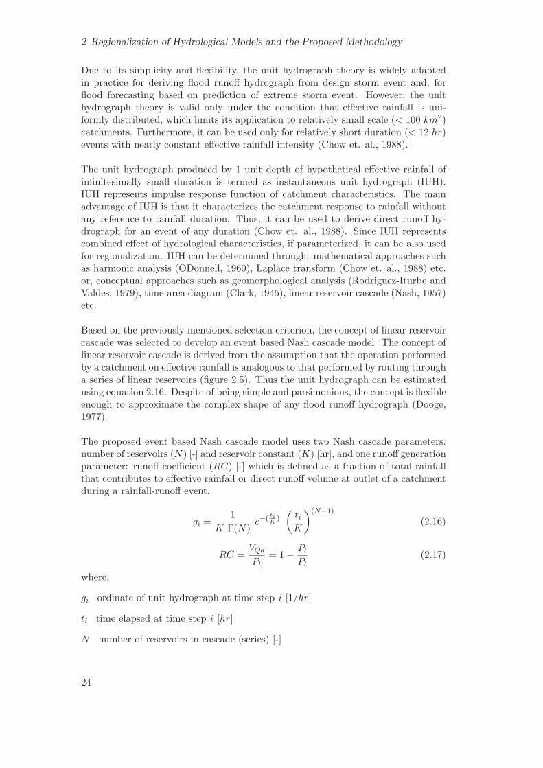
2 Regionalization of Hydrological Models and the Proposed Methodology
Due to its simplicity and flexibility, the unit hydrograph theory is widely adaptedin practice for deriving flood runoff hydrograph from design storm event and, forflood forecasting based on prediction of extreme storm event. However, the unithydrograph theory is valid only under the condition that effective rainfall is uni-formly distributed, which limits its application to relatively small scale (< 100 km2)catchments. Furthermore, it can be used only for relatively short duration (< 12 hr)events with nearly constant effective rainfall intensity (Chow et. al., 1988).
The unit hydrograph produced by 1 unit depth of hypothetical effective rainfall ofinfinitesimally small duration is termed as instantaneous unit hydrograph (IUH).IUH represents impulse response function of catchment characteristics. The mainadvantage of IUH is that it characterizes the catchment response to rainfall withoutany reference to rainfall duration. Thus, it can be used to derive direct runoff hy-drograph for an event of any duration (Chow et. al., 1988). Since IUH representscombined effect of hydrological characteristics, if parameterized, it can be also usedfor regionalization. IUH can be determined through: mathematical approaches suchas harmonic analysis (ODonnell, 1960), Laplace transform (Chow et. al., 1988) etc.or, conceptual approaches such as geomorphological analysis (Rodriguez-Iturbe andValdes, 1979), time-area diagram (Clark, 1945), linear reservoir cascade (Nash, 1957)etc.
Based on the previously mentioned selection criterion, the concept of linear reservoircascade was selected to develop an event based Nash cascade model. The concept oflinear reservoir cascade is derived from the assumption that the operation performedby a catchment on effective rainfall is analogous to that performed by routing througha series of linear reservoirs (figure 2.5). Thus the unit hydrograph can be estimatedusing equation 2.16. Despite of being simple and parsimonious, the concept is flexibleenough to approximate the complex shape of any flood runoff hydrograph (Dooge,1977).
The proposed event based Nash cascade model uses two Nash cascade parameters:number of reservoirs (N) [-] and reservoir constant (K) [hr], and one runoff generationparameter: runoff coefficient (RC) [-] which is defined as a fraction of total rainfallthat contributes to effective rainfall or direct runoff volume at outlet of a catchmentduring a rainfall-runoff event.
gi =1
K Γ(N)e−(
tiK
)
(tiK
)(N−1)
(2.16)
RC =VQd
Pt= 1 − Pl
Pt(2.17)
where,
gi ordinate of unit hydrograph at time step i [1/hr]
ti time elapsed at time step i [hr]
N number of reservoirs in cascade (series) [-]
24

2.3 The proposed methodology
K retention time of reservoirs [hr]
RC runoff coefficient [-]
VQd specific direct runoff volume [mm]
Pt total rainfall during an event [mm]
Pl rainfall loss occurred during an event [mm]
Figure 2.5: Concept of Nash cascade linear reservoirs
The model setup
To capture heterogeneity of hydrological characteristics to a better extent by avoid-ing averaging over larger areas, the model setup (figure 2.6) is implemented at thesubcatchment scale of 50 km2 to 75 km2. Various methods, such as runoff coef-ficient method, constant or variable loss rate method etc., are commonly appliedto estimate effective rainfall at each time interval of a rainfall-runoff event. In theproposed model setup effective rainfall at hourly time intervals is estimated usingconstant loss rate method (equation 2.18). Then, as shown in equation 2.19, theeffective rainfall time series for each subcatchment is transformed into hourly directrunoff hydrograph using the Nash cascade parameters for the respective subcatch-ment. Finally, the direct runoff hydrographs for the subcatchments are routed tooutlet of the catchment using flood routing procedure.
The model setup and the flood routing procedure was encoded into computer programusing the FORTRAN programming language.
Pe(i,j) = P(i,j) − φj (2.18)
25

2 Regionalization of Hydrological Models and the Proposed Methodology
Qd(i,j) =i∑
l=1
Pe(i−l+1,j) Aj
3.6 Kj Γ(Nj)e−
(tl
Kj
) (tlKj
)(Nj−1)
(2.19)
where,
P(i,j) rainfall at time step i at outlet of subcatchment j [mm/hr]
Pe(i,j) effective rainfall intensity at time step i at outlet of subcatchment j [mm/hr]
φ rainfall loss rate [mm/hr]
Nj number of reservoirs in cascade for subcatchment j [-]
Kj reservoir constant for subcatchment j [hr]
Qd(i,j) direct runoff at time step i at outlet of subcatchment j [m3/s]
Aj area of subcatchment j [km2]
Figure 2.6: Semi-distributed, event based Nash cascade model
26

2.3 The proposed methodology
2.3.2 Flood routing
Flood routing is necessary in order to account for change in the shape of runoff hydro-graph during its propagation from outlet of a subcatchment to outlet of a catchment.The Muskingum flood routing procedure was adopted for the proposed model setupbecause of its simplicity and less data requirement (Tung, 1985; Gill, 1978). Musk-ingum routing procedure estimates the outflow at the end of a river stretch usingequations 2.20 to 2.24 and the two routing parameters: retention constant (km) [s]and weighting factor (xm) [-].
Qouti = C1Qini + C2Qini + C3Qouti−1 (2.20)
C1 = − kmxm − 0.5∆t
km(1 − xm) + 0.5∆t(2.21)
C2 =kmxm + 0.5∆t
km(1 − xm) + 0.5∆t(2.22)
C3 =km − kmxm − 0.5∆t
km(1 − xm) + 0.5∆t(2.23)
C1 + C2 + C3 = 1 (2.24)
where,
Qouti outflow of at the end of river channel at time step i [m3/s]
Qini inflow of at the beginning of river channel at time step i [m3/s]
km Muskingum retention constant of river channel [s]
xm Muskingum weighting factor [-]
In the case of gauged catchments, the Muskingum routing parameters km and xm
can be estimated through calibration. But for ungauged catchments, the parametersmust be estimated using the Muskingum-Cunge (Chow, 1988) method, as shownin equations 2.25 and 2.26. Muskingum-Cunge method uses flow and river channelcharacteristics to estimate the parameters, these characteristics are usually derivedfrom morphological data. However in the case of this study, due to lack of the mor-phological data, direct application of Muskingum-Cunge method was not possible.Tewolde and Smithers (2006) demonstrated an empirical approach (equations 2.27 to2.32) to estimate the flow and river channel characteristics where no morphologicaldata is available. The empirical approach was used to estimate the flow and riverchannel characteristics, which can be then inserted into Muskingum-Cunge equationsto obtain the routing parameters km and xm.
km =L
Vw(2.25)
xm =1
2− Qr
2sPwVwL(2.26)
27

2 Regionalization of Hydrological Models and the Proposed Methodology
Qr = Qb + 0.5(Qp −Qb) (2.27)
Pw = 3.82√Qr (for cohesive river bed) (2.28)
y =
(Qr
0.508Pw√s
)( 3
5)
(2.29)
R =2y
3(for wide parabolic channels) (2.30)
Vav =R( 2
3)√sn
(2.31)
Vw =11Vav
9(for wide parabolic channels) (2.32)
where,
Qr reference discharge [m3/s]
Qb base flow [m3/s]
Qp peak flow [m3/s]
Pw weighted perimeter [m]
y flow depth [m]
R hydraulic mean depth [m]
Vav average velocity [m/s]
s slope of river channel [-]
L length of river channel [-]
n Manning’s roughness coefficient [-] (here, n=0.035)
Vw celerity [m/s]
2.3.3 Regionalization of the model parameters
Among the three model parameters of the proposed event based Nash cascade model,runoff coefficient RC deals with runoff generation, on the other hand Nash cascadeparameters N and K represent runoff propagation. The two processes are inde-pendent of each other, hence, RC can be treated independent of N and K. Thisfacilitates to break up the regionalization procedure of the model parameters intointo two steps.
Since the parameter RC is independent of the other two parameters, the parameteridentification (equifinality) problem does not exist for RC. In the case of gauged
28

2.3 The proposed methodology
catchments, RC for an event can be calculated from “observed” direct runoff volumefor the event. However, in the case of ungauged catchments where the observed runoffhydrograph is not available, the direct runoff volume must be determined indirectlyby deducting rainfall loss from the total rainfall occurred during the event. Rain-fall loss occurred during an event represents infiltration and interception of rainfall,which directly depends upon catchment and event specific hydrological characteris-tics. Thus, there is a possibility to estimate rainfall loss through the regional transferfunction approach. Therefore, it is intended to derive a transfer function for rainfallloss which can be then used to calculate RC as shown in equation 2.17. Four dif-ferent possibilities, using purely data driven as well as data-plus-knowledge drivenapproaches, were investigated to obtain a robust and physically reasonable transferfunction for rainfall loss.
On the other hand, in the case of Nash cascade parameters N and K, it has beenobserved that calibrating parameters for a rainfall-runoff event in a catchment mayresult in large number (> 100) of parameter sets yielding equally high model per-formance (Bardossy, 2007), which underlines the strong interaction between the twoparameters. Therefore, to derive transfer functions for the Nash cascade parame-ters, a different approach was employed. The approach is aimed at exploiting theinter-parameter relationship to reduce the uncertainty due to parameter identifica-tion problems. Furthermore, it is intended to derive regionally optimum solution byoptimizing the regional performance of the transfer functions.
The regionalization procedures for the three parameters of the event based Nashcascade model and the respective results are discussed in details in chapter 4 andchapter 5.
29

3 Overview of the Study Area and the
Hydrological Characteristics
3.1 General description of the study area
The study under discussion was carried out over the south-west region of Ger-many (figure 3.1). The region is governed under the state authorities of Baden-Wuerttemberg. Stuttgart, Karlsruhe and Tuebingen are the major urban settlementsin the region. The main rivers in the region are Rhein, Danube and Neckar. TheRhein river forms western boundary of the region and the Neckar flows through cen-tral part of the region to meet the Rhein at Manheim. The 367 km long stretch ofthe Neckar divides the region into western and eastern parts. The western part iscovered with the Black Forest and the eastern part stretches over the Swabian Alps.The selected catchments form major part of the Rhein basin; 13,000 (km2) of whichis drained through the Neckar and the remaining through various small tributaries.A small part of the study area drains into the Danube which flows along the south-east foothill of the Swabian Alps.
The region extends over wide range of landscape features. Although in the South itexhibits highly varying altitudes, the cities on the North are situated in the relativelyflat valley of the Neckar river. Topographic elevation in the region ranges from 124m.a.s.l to 1487 m.a.s.l. with a mean elevation of about 600 m.a.s.l. Although maxi-mum slopes in parts of Black Forest and the Swabian Alps are as high as 150 %, themean slope in the region is only 15 %, with 90 % of the slopes are within range of 0% to 32 %.
The oldest geologic formations in the region are the variegated sandstone forma-tions. The variegated sandstone formations are covered with variety of sedimentformations from the Jurassic and the Triassic periods which are predominantly com-posed of malm, doggerlime, keuper, shelly limestone and sandstone. Some parts atthe foothill of the Swabian Alp are composed of karstic rock formations. The karsticrock formations act as interconnected subsurface reservoirs causing considerably largeamount of subsurface water transfer from one catchment to another catchment onrelatively short time scale. The subsurface flow directions are not yet fully under-stood which often leads to discrepancies in water balance calculations for the region.
Variations in the soil cover of the region is a direct consequence of the geological vari-ability. Soil cover in the area of the Black Forest, which is made of shallow podsolsand grey brown podsols, is formed by weathered variegated sandstones. The easternareas are covered with layers of loess, sandy soils as well as heavy clay originatedfrom shelly limestone and keuper formations.
30

3.2 Data situation of the study area
The dominating vegetation in the region is forest of spruce, fir and beech. The fer-tile areas on the either banks of the Neckar and foothills of the Swabian Alps aremostly used for agriculture, pasture and meadows. The slopes of the Swabian Alpsare partly used for cultivation of wine yards, fruits etc. and partly covered with ash,beech and elm trees. The barren soil on the top of the Swabian Alps is covered withheath and juniper.
The climate of the region is influenced by both continental as well as oceanic weathersystems. But due to western wind flowing through the region, the impact of theAtlantic Ocean is relatively higher. The weather is characterized by warm-to-hotsummers and mild winters. The minimum average temperature in the region is esti-mated to be −0.5oC in January and the maximum average temperature to be 17.3oCin July. The annual mean potential evapotranspiration is estimated to be 560 mm,with the minimum monthly potential evapotranspiration of about 10 mm in Januaryand the maximum monthly potential evapotranspiration of about 90 mm in July.
Mean annual rainfall in the region ranges from 740 mm near Stuttgart to 1790 mmin the Black Forest with spatial mean of 1160 mm. Mean summer rainfall and themean winter rainfall are respectively estimated to be 645 mm and 520 mm. FromDecember to April precipitation usually occurs as snow fall, most of the runoff eventsoccurring during this period can be attributed to snow melt. The runoff events in themonths of July, August and September can be attributed to east bound advectivestorm coming from the Atlantic Ocean.
The above mentioned description of the study area is based on the descriptionsprovided by Bardossy et. al. (1999), Patil (2004) and Das (2006).
3.2 Data situation of the study area
The meteorological, hydrological and landscape data for the region was providedby German Weather Service (DWD) and State Agency for Environmental Protec-tion, Baden-Wuerttemberg (LFU-BW). Detailed description of the available data ispresented in table 3.1.
3.3 Selection of catchments and events
The crucial criteria behind the selection of the catchments was the availability of thehydrological data at required spatial and temporal resolution. During the selection,only the mesoscale catchments with area ranging for 50 km2 to 1000 km2 were con-sidered. The catchments influenced by hydraulic control structures and hydro-powerplants were deliberately neglected.
With the intention to cover the wide extent of the regional characteristics, 41 catch-ments were selected across the region. Twenty one of the selected catchments draininto the Neckar, 17 catchments drain into the Rhein through various small tributaries
31

3 Overview of the Study Area and the Hydrological Characteristics
Figure 3.1: Overview of the study area and selected catchments
32

3.3 Selection of catchments and events
Table 3.1: Description of the available data
Data Time Number of Temporal Spatial/period stations scale Scale
Discharge time series 1974-2003 41 hourly -Rainfall time series 1980-2003 212 hourly 1 station/180 km2
Rainfall time series 1958-2003 475 daily 1 station/80 km2
Digital elevation map - - - 30 m x 30 mLand use (10 classes) 1975 - - 50 m x 50 mLand use (16 classes) 1993 - - 30 m x 30 mLand use (16 classes) 2000 - - 30 m x 30 mSoil classification map - - - 1:600,000Stream flow network - - - 1:500,000
and the rest 3 directly drain into the Danube.
Standard split sampling method was used for the optimization and validation of theregionalization methodology. It was assumed that the region is relatively homoge-neous and the selected catchments are relatively similar. Hence regionalization andvalidation sets were formed by randomly distributing the catchments into the eithersets. Out of the 41 catchments, 22 catchments (regionalization set: catchments 1-22 in table 3.2) were used to set up and to optimize the proposed regionalizationmethodology and rest 19 catchments (validation set: catchments 23-41 in table 3.2)were used for validation of the regionalization methodology.
More than 200 large rainfall-runoff events, which occurred during the period from1989 to 2003, were selected from the catchments. Out of them, 104 events belong tothe regionalization set and 105 events belong to the validation set. In order to avoidsnow melt events, the events occurred during the period from beginning of Decemberto end of April were not considered for the selection. The table 3.4 shows the statisticsof hydrological characteristics for the regionalization and validation sets. Figure 3.2and 3.3 show overview of the spatial distribution of highest and mean specific peakrunoff (qpeak) [mm/hr] for the events selected from each catchments.
3.3.1 Estimation of rainfall
The event based Nash cascade model needs input of hourly rainfall time series lumpedat subcatchment scale. In order to estimate the rainfall input for the subcatchments,it was essential to interpolate the point measurements of rainfall to grid cells. Theinterpolation was carried out by using a external drift kriging procedure (Ahmed andMarsily, 1987). To account for the orographic effect on the rainfall fields, square oftopographic elevation was used as the external drift variable.
Initially, only hourly rainfall data was used for the estimations. However, it was
33

3 Overview of the Study Area and the Hydrological Characteristics
Table 3.2: Summary of the selected Catchments
Catchment Catchment Area Number of Number ofnumber name (km2) subcatchments events
1 Zell am Harmersbach 103 2 12 Tegernau 70 2 93 Untermunstertal 66 2 84 Kappelrodeck 53 2 65 Steinheim 76 2 66 Rangendingen 123 2 67 Iselshausen 147 3 68 Lautenhof 85 2 59 Gollsdorf 124 3 510 Lahr 130 3 511 Zell 206 4 512 Horgen-Klaranlage 208 3 513 Hinterlehengericht 106 2 414 Pfaffingen 134 3 415 Oppenweiler 181 3 416 Owingen 206 4 417 Neuenstadt 141 3 318 Oberensingen 178 4 319 Ewattingen 341 7 220 Plochingen 704 12 221 Unterschmeien 151 3 122 Mosbach 156 3 123 Baden-Baden 71 2 724 Schenkenzell 76 2 925 Haubersbronn 77 2 126 Tuttlingen 81 2 427 St. Blasien 97 2 928 Huttlingen 107 2 329 Ramsbach 108 2 830 Oberwolfach 126 2 731 Tubingen 141 3 432 Gutach 145 3 833 Ettlingen 149 4 334 Riederich 160 3 335 Wannweil 161 3 836 Hammereisenbach 164 3 637 Talhausen 192 3 738 Eschelbronn 198 4 439 Hopfau 202 4 940 Berghausen 232 5 141 Schafhausen 238 5 4
34

3.3 Selection of catchments and events
Figure 3.2: Maximum spec. peak runoff Figure 3.3: Mean spec. peak runoff
Figure 3.4: Maximum total rainfall Figure 3.5: Mean total rainfall
35

3 Overview of the Study Area and the Hydrological Characteristics
observed that the hourly rainfall data, although representing temporal distributionof the rainfall quite well, leads to frequent underestimations of amount of rainfall.Figure 3.6 shows the interpolated rainfall and the direct runoff hydrograph for oneof the selected rainfall-runoff events. It can be observed that, although the temporaldistribution of the interpolated rainfall is correlated with the direct runoff, the specificvolume of the interpolated rainfall (4.4 mm) is actually less than the specific directrunoff volume (5.1 mm) for the event. This is due to the fact that the network ofthe hourly rainfall measurement stations is not dense enough to capture the spatialdistribution of the rainfall fields. On the other hand, density of the daily rainfallmeasurement stations is high, and allows for the capture of spatial distribution ofthe daily rainfall fairly well. Hence, the daily rainfall (Pdly) [mm] at each grid cell,was weighted by the hourly rainfall (Phr) [mm] at the grid cell, as shown in equation3.1, to disintegrate the daily rainfall into hourly time step. Thus, modified rainfallestimations, although do not solve the problem completely, lead to improvement overthe previous estimations. The corrected lumped hourly rainfall time series (Phr,corr)[mm] was then used as the main input for the event based model.
Figure 3.6: Interpolated hourly rainfall and corrected hourly rainfall
Pi,hr,corr =Pi,hr∑24
j=1 Pj,hr
· Pdly (3.1)
3.4 Estimations of hydrological characteristics
To capture the heterogeneity of the hydrological characteristics to a better extentby avoiding averaging over larger areas, the selected catchments were divided intosubcatchments of size 50 km2 to 75 km2. Estimation of the hydrological charac-teristics was carried out at the subcatchment scale using the data set mentioned
36

3.4 Estimations of hydrological characteristics
in the table 3.1. Delineation of the subcatchments and drainage network as wellas estimation of the spatial hydrological characteristics was carried out using GIStools. The various hydrological characteristics are classified into two groups: eventspecific characteristics and catchment specific characteristics. The relevance of thehydrological characteristics to rainfall-runoff processes and their estimations are dis-cussed in the following sections. Statistics of the hydrological characteristics for theregionalization and validation sets are given in table 3.4, at the end of this chapter.
3.4.1 Event specific characteristics
Event specific characteristics are those which are dependent on the rainfall-runoffevent and the conditions prior to the event. The event specific characteristics includetotal rainfall, event duration, season, antecedent moisture conditions etc. Due tothe fact that hydrological conditions in a catchment are continuously alternating,response of a catchment to two identical but temporally separate rainfall eventscan be very different from each other (Beven, 2001). Therefore, while modelingrainfall-runoff processes, it is crucial to account for the event specific conditions ofa catchment. Inclusion of the event specific characteristics in the regional transferfunctions may also facilitate temporal extrapolation of the model parameters.
Total rainfall and duration
Total rainfall and the duration of a rainfall event may have a significant influenceon the runoff generation process during the event. Higher total rainfall may lead toa larger runoff coefficient (RC) [-]. On the other hand, longer event duration maylead to smaller runoff coefficients. The influence of total rainfall and duration on therunoff propagation is, however, not yet fully understood. Total rainfall (Pt) [mm]and duration (Tp) [hr] were estimated for the selected rainfall-runoff events using therespective rainfall time series. Figure 3.4 and 3.5 show the spatial distribution ofmaximum and mean total event rainfall for the events selected from each catchment.
Season
The season of a rainfall-runoff event can be represented by the month (M) of occur-rence of the event. Seasonal variations in the catchment conditions such as soil mois-ture, temperature, vegetation etc. greatly influence the runoff generation process.The summer months lead to smaller runoff coefficient due to presence of vegetationand rapid evaporation. On the other hand, saturated soil conditions and the lack ofvegetation in the winter, often lead to a larger runoff coefficient.
Antecedent precipitation index
The soil moisture condition prior to a rainfall event has great influence on runoffgeneration process, higher moisture content, generally, leads to a higher runoff gener-ation (Chow, 1988) and vice versa. Exact soil moisture condition prior to a rainfall-runoff event, practically, cannot be determined. Hence, antecedent precipitationindex (API) [mm] is often used as a measure of the soil moisture condition. An-tecedent precipitation index is based on the assumption that soil moisture after a
37

3 Overview of the Study Area and the Hydrological Characteristics
rainfall event decreases exponentially. The more time elapsed after rainfall is ceasedthe less moisture remained in soil due to evaporation and infiltration losses. The an-tecedent precipitation index can be calculated using equation 3.2. The decay factorλ normally ranges between 0.85 and 0.98, depending on the catchment or the region.However, most of the empirical investigations suggest λ = 0.90 which was commonlyused for all the catchments under consideration. The impact of rainfall preceding anevent by more than 7 days was not considered (n = 7 days).
API(t0) =n∑
i=1
Pdly(t0−i) · λi (3.2)
3.4.2 Catchment specific characteristics
Catchment specific characteristics are those which do not change significantly withtime or event, however, may vary with respect to spatial location. The catchmentspecific characteristics include catchment shape, morphology, topography, soil prop-erties etc. Rainfall-runoff processes in a catchment are chiefly governed by the catch-ment specific characteristics, most of the existing regionalization methods associatethe model parameters only with catchment characteristics. Thus, the relationshipbetween model parameters and catchment specific characteristics facilitates spatialextrapolation or regionalization of the model parameters.
Area and perimeter
Form of a catchment, which can be expressed in terms of its area (A) [km2] andperimeter (Per) [km], may considerably influence runoff generation as well as prop-agation process in the catchment. The larger area and perimeter of a catchment, thelonger traveling distances and the subsequent retention time which leads to higherrainfall loss and delayed arrival of runoff at outlet of the catchment.
Shape factor
The shape factor (SF ) [-] is an approximate representation of shape of a catchmentin the form of ratio of area of the catchment and square of length of the longest pathin the catchment. For two catchments with equal areas, a smaller value of the shapefactor means an elongated catchment and larger values are representative of fan-shaped catchments. Elongated catchments usually exhibit longer time to occurrenceof peak runoff due to longer flow paths, on the other hand a compact fan-shapedcatchment may cause quick runoff concentration at its outlet.
SF =A
L2l
(3.3)
Mean slope
Runoff generation process, surface and groundwater flow patterns are greatly influ-enced by the topographic patterns in a catchment (Beven, 2001). Surface slope isthe most prominent variable through which catchment topography can be expressed.
38

3.4 Estimations of hydrological characteristics
Steep slopes in a catchment cause faster runoff propagation, thus may lead to largerunoff volume and high peak runoff. Local slopes for each grid cell were calculatedfrom the digital elevation map by means of GIS tools, then the mean slope (SL) [-] ofeach subcatchment was estimated by taking spatial average of the grid based slope.The spatial distribution of SL for the catchments is shown in figure 3.7.
Mean topographic wetness index
Topographic wetness index is the variable that describes topographical patterns, itrepresents the propensity of any point in a catchment to develop saturated conditions(Beven, 2001). Topographic wetness index for a point is expressed as a ratio of thedrainage area (a) to upstream of a point to the local topographic slope (tanβ), asshown in equation 3.4. Topographic wetness index was used in TOPMODEL (Bevenand Kirkby, 1979) to predict saturated areas contributing to runoff generation ateach time step. In equation 3.5, a negative value of Di indicates that the area issaturated and saturation overland flow is generated. A positive value of Di indi-cates that there is a storage deficit. Thus, each point with the same topographicwetness index behaves functionally in an identical manner (Beven, 2001). Therefore,topographic wetness index may represent the hydrological similarity. High values ofthe topographic wetness index means either large drainage area or flat slope anglesleading to a large storage potential. Thus, a high topographic wetness index mayresult in a small runoff coefficient and slower runoff propagation. Mean topographicwetness index (TWI) [-] for each subcatchment was calculated by averaging gridbased topographic wetness index. Figure 3.8 shows the spatial distribution of TWIfor the catchments.
twi = ln(a
tanβ) (3.4)
Di = D +m[TWI − ln(a
tanβ)] (3.5)
twi topographic wetness index [-]
TWI mean topographic wetness index [-]
a drainage area to upstream of a point in a catchment [m2]
tanβ local topographic slope at the point [-]
Di local storage deficit at the point and time step i [m]
D mean storage deficit over a catchment [m]
m change in transmissivity with depth [m]
Terrain ruggedness index
Terrain ruggedness index represents the terrain roughness. Terrain ruggedness indexfor a grid cell is expressed as root mean of the sum of squared elevation differences be-tween the grid cell and its 8 adjacent cells in digital elevation map (Riley et. al., 1999).Higher terrain ruggedness may cause longer retention time, which consequently may
39

3 Overview of the Study Area and the Hydrological Characteristics
lead to smaller runoff coefficient and longer travel time. Terrain ruggedness index foreach grid cell was calculated using equation 3.6, then the grid based index was aver-aged over respective subcatchments to obtain mean terrain ruggedness index (TRI)[m]. The spatial distribution of TRI is shown in figure 3.9.
TRIi =
√∑8j=1(Elvi − Elvj)2
8(3.6)
TRIi terrain ruggedness index for grid cell i
Elvi elevation of grid cell i
Elvj elevation of jth adjacent cell
River density
River density represents network of river streams in a catchment. It is expressed asratio of sum of lengths of all river streams (Li..n) in a catchment and area of thecatchment (A). River density is highly correlated with runoff generation process, adense river network results in higher runoff generation and faster runoff propagation(Patil, 2004). The line density method illustrated by Silvermann (1986) was used toestimate the river density (DR) [1/km] for the subcatchments. Figure 3.10 showsthe spatial distribution of DR.
DR =
∑ni=1 Li
A(3.7)
Time of concentration
Time of concentration is the time after which runoff produced at the farthest pointfrom the outlet of a catchment, reaches the outlet. Theoretically, it represents thetime at which runoff from complete area of the catchment under constant rainfallbegins to concentrate at the outlet and the runoff curve reach at its peak. For smallcatchments time of concentration is very close to time to occurrence of peak runoffat outlet, but for large catchments it is often greater than the time to occurrenceof peak runoff. However, time of concentration usually exhibits high correlationswith time to occurrence of peak runoff at outlet and the peak runoff itself. Time ofconcentration (TC) [hr] can be estimated by means of the Kirpich formula (equation3.8; Kirpich, 1940) using the longest flow path in the catchment (Ll) [m] and slopeof the longest flow path (S).
TC = 0.0003245 · L0.77l
S0.385(3.8)
Soil classes based on hydraulic conductivity
Infiltration of rainfall into the soil surface directly depends upon vertical hydraulicconductivity [mm/hr] of the soil (Chow, 1988), hence, vertical hydraulic conductiv-ity of soil plays significant role in runoff generation process. Higher vertical hydraulic
40

3.4 Estimations of hydrological characteristics
Figure 3.7: Mean slope Figure 3.8: Mean top. wetness index
Figure 3.9: Mean top. ruggedness index Figure 3.10: Mean river density
41

3 Overview of the Study Area and the Hydrological Characteristics
conductivity may lead to higher infiltration losses, consequently, smaller runoff vol-ume. The available soil map is provided with 10 soil classes based on the fieldmeasurement of vertical hydraulic conductivity, the soil classes were reclassified intothree classes, ranging from low to high hydraulic conductivity as shown in table 3.3.Relative areas of the soil classes (Kv) were used as the hydrological variables to de-scribe the hydraulic conductivity. The spatial distribution of the soil classes is shownin figure 3.11.
Table 3.3: Soil classes based on hydraulic conductivity
Notation Hydraulic conductivity Class(mm/hr)
Kv1 < 42 lowKv2 42-292 mediumKv3 > 292 high
Field capacity
Field capacity of soil is the maximum amount of water per unit area that can beretained by the soil against the force of gravity. The infiltration rate of soil is alsorelated to its field capacity, higher field capacity may lead to lower runoff generationdue to large volume of water retained in the soil. Approximate estimations of meanfield capacity (FCm) [m] for the subcatchments were obtained from the available soilmap. The spatial distribution of FCm is shown in figure 3.12.
Land use classes
Recent studies conclude that there are clear indications of effects of land use changeson rainfall-runoff processes (Hundecha and Bardossy, 2004). Increases in the amountof urban area or decreases in forest area leads to higher runoff generation and fasterrunoff propagation. Thus, deforestation and urbanization have led to increase inflood severity to disastrous levels. Hence, it was inevitable to incorporate land usecharacteristics in the proposed regionalization methodology. For simplification the16 land use classes of the original data sets were reorganized into four classes: Forest(LUf ), Urban (LUu), Agriculture (LUa) and water bodies (LUw). Unlike the othercatchment specific characteristics, land use is likely to change not only with spacebut also with time. Therefore, the relative area of each land use class for each eventwas estimated through linear interpolation or extrapolation between the land use foryear 1993 (figure 3.13) and year 2000 (figure 3.14).
42

3.4 Estimations of hydrological characteristics
Figure 3.11: Soil classes Figure 3.12: Mean field capacity
Figure 3.13: Land use in year 1993 Figure 3.14: Land use in year 2000
43

3 Overview of the Study Area and the Hydrological Characteristics
Table 3.4: Statistics of the hydrological characteristics (HCs)
Regionalization set Validation set(22 catchments, 104 events) (19 catchments, 105 events)
HCs Max Min Mean Std dev Max Min Mean Std dev
event specific characteristics
qpeak 3.78 0.12 0.58 0.49 3.51 0.12 0.79 0.71Pt 45.6 4.4 17.6 9.2 80.8 4.2 22.0 14.9Tp 26.0 2.0 8.9 4.9 38.0 2.0 11.6 6.5API 26.7 0.00 11.2 6.9 84.2 0.73 15.4 13.6
catchment specific characteristics
A 53 693 158 125 71 337 154 68Per 43 229 90 36 50 163 92 29SL 0.05 0.31 0.15 0.08 0.06 0.27 0.14 0.06TWI 4.28 6.06 5.16 0.52 4.43 6.00 5.18 0.48TRI 4.95 31.04 14.20 7.60 5.37 26.41 13.58 6.27DR 0.38 1.74 1.08 0.30 0.68 1.68 1.07 0.30TC 1.03 6.01 2.77 1.05 1.53 4.00 2.72 0.72SF 0.10 0.37 0.23 0.08 0.11 0.39 0.22 0.07Kv1 0.00 0.93 0.20 0.34 0.00 0.96 0.39 0.35Kv2 0.00 0.91 0.31 0.33 0.00 0.91 0.30 0.28Kv3 0.00 0.07 0.01 0.02 0.00 0.01 0.00 0.00FCm 0.00 3.10 1.24 1.14 0.00 3.52 1.11 0.83LUf 0.17 0.94 0.55 0.18 0.30 0.88 0.58 0.19LUu 0.00 0.11 0.02 0.03 0.00 0.05 0.02 0.01LUa 0.00 0.23 0.01 0.05 0.00 0.67 0.26 0.19
44

4 Regionalization of Rainfall Loss
4.1 Runoff coefficient
A runoff hydrograph can be separated into two types of runoff sources: base flowand direct runoff. Base flow is the part of rainfall that infiltrates into the soil. Theinfiltrated rainfall water flows horizontally either through soil layer as subsurfacewater or along the confining geological formation as groundwater. If the flow comesacross a river channel, a portion of it joins the river as base flow. Direct runoff is theportion which flows over the land surface, it can be attributed to either Hortonianoverland flow or saturated overland flow (Chow et. al., 1988). Hortonian overlandflow occurs when rainfall intensity exceeds infiltration rate and saturated overlandflow occurs when soil is completely saturated.
Since subsurface flow and groundwater flow move much slower as compared to over-land flow, the effects of base flow produced during a rainfall-runoff event may occurin rivers several hours, days, or even weeks after the event. Therefore the contri-bution of base flow to flood runoff is often very small as compare to that of directrunoff. The flood runoff hydrograph for a rainfall-runoff event is usually dominatedby direct runoff. Hence, for estimations of flood runoff volume only direct runoff isconsidered and the amount of rainfall infiltrated into the soil is treated as rainfallloss. The amount of rainfall which forms the overland flow and contributes to thedirect runoff at each time step of a rainfall-runoff event is referred as effective rainfallintensity (Pe). To derive a direct runoff hydrograph for a given rainfall-runoff event,the total direct runoff volume and the effective rainfall intensity at each time step ofthe event must be known.
The runoff coefficient (RC) for a rainfall-runoff event represents the fraction of to-tal rainfall that contributes to the direct runoff at the outlet of a catchment. Itis expressed as the ratio between the total direct runoff and the total rainfall oc-curred during the event (equation 4.1). If the runoff coefficient is known, the directrunoff volume and the corresponding effective rainfall intensity at each time step ofa rainfall-runoff event can be estimated using either runoff coefficient method (figure4.1) or constant loss rate (φ-index) method (figure 4.2).
RC =VQd
Pt= 1 − Pl
Pt(4.1)
RC runoff coefficient for an event [-]
VQd specific direct runoff volume [mm]
Pt total rainfall during the event [mm]
45

4 Regionalization of Rainfall Loss
Figure 4.1: Runoff coefficient method Figure 4.2: Constant loss rate method
Pl rainfall loss during the event [mm]
P rainfall intensity during the event [mm/hr]
Pe effective rainfall intensity [mm/hr]
φ constant rainfall loss [mm/hr]
In the case of gauged catchments, the runoff coefficient can be estimated by usingthe observed direct runoff volume. “Observed” direct runoff volume can be obtainedfrom observed runoff hydrograph by means of a simple straight line hydrograph sep-aration method as shown in figure 4.3.
However, in the case of ungauged catchments, where observed runoff hydrographis not available, direct runoff volume must be determined indirectly by deductingrainfall loss from total rainfall occurred during an event. Rainfall losses representinfiltration of rainfall into soil, and to some extent the interception of rainfall due tothe presence of vegetation. Rainfall loss occurred during an event directly dependsupon the catchment as well as event specific hydrological characteristics. Therefore,there is a possibility to estimate rainfall loss through the regional transfer functionapproach based on catchment as well as event specific hydrological characteristics.Then, estimated rainfall loss can be used to calculate direct runoff volume and runoffcoefficient.
4.2 Transfer function for rainfall loss
Several different approaches can possibly be adopted to derive the transfer functionthat associates rainfall loss with the hydrological characteristics. The approachescan be classified into two categories: purely data driven approaches and data-plus-knowledge driven approaches.
46

4.2 Transfer function for rainfall loss
Figure 4.3: Straight line hydrograph separation method
Purely data driven approaches derive the functional relationship between predictorsand a response variable solely from an observed dataset, by calibrating (or regress-ing) the coefficients of a convenient functional form to achieve desired degree ofgoodness fit between calculated and observed response. The purely data driven ap-proaches do not take account of the physical relationships between predictors and aresponse variable. One other hand, data-plus-knowledge driven approaches exploita priori knowledge of the physical relationships to guide the derivation of the func-tional relationships between predictors and a response variable. The coefficients ofsuch, physically reasonable, functional relationships are derived through calibration(or regression) against observed response. Thus, the data-plus-knowledge driven ap-proaches are partially deterministic.
The purely data driven approaches, such as artificial neural networks, are excellentat fitting the observed response with calculated response. Mainly, because of theirextreme flexibility which is able to replicate non-linear relationships. However, dueto the lack of physical basis purely data driven approaches may lead to erroneousand potentially counterfactual predictions, especially for extrapolation beyond therange of the data which was used for its derivation. To obtain efficient and plausibleregionalization, it is important that the transfer function, not only replicates non-linear relationships but also appropriately represents physical relationships betweenpredictors and the response variable.
During this study, four different approaches were employed to derive four different
47

4 Regionalization of Rainfall Loss
transfer functions for rainfall loss. Three of them are purely data driven approachesbased on multiple linear regression, the artificial neural network (ANN) and fuzzylogic. The fourth approach is a data-plus-knowledge driven approach based on lo-gistic regression. The rainfall-runoff events in the regionalization set (see: section3.3) were used to derive and optimize the transfer functions. Validation of spatialtransferability of the transfer functions was carried out using the validation set ofthe events. The “observed” direct runoff volume and the corresponding rainfall lossfor the events was estimated using the straight line hydrograph separation method(figure 4.3).
The derivation procedure for the transfer functions using the four approaches, theirgoodness fit performance and aptness with respect to the physical relationships un-derlying rainfall loss processes are discussed in the following part of the chapter.
4.2.1 Multiple Linear Regression
Multiple linear regression (MLR) is a classic approach to fit a multivariate linearfunction between a response variable and a set of more than one predictors. Amultivariate linear function (equation 4.2) between response variable Y and pre-dictors X1, X2, ..., Xn comprises of an intercept β0 and coefficients β1, β2, ..., βn
corresponding to each of the predictors. The intercept and the coefficients must beestimated through a regression procedure.
Y = β0 + β1X1 + β2X2 + ...+ βnXn (4.2)
The simulated annealing optimization algorithm (Kirkpatrick et. al., 1983) wasadopted to carry out the multiple linear regression procedure. The optimizationalgorithm was aimed at minimizing the root-mean-squared error (RMSE; equation4.3) and maximizing the correlation coefficient (Corr) between the observed rainfallloss (Pl,ob) and the calculated rainfall loss (Pl,ca) for n = 104 number of events in theregionalization set.
Minimize
RMSE =
√∑ni=1 (Pl,ob − Pl,ca)
2
n
(4.3)
Initially, 14 probable predictors, describing various event and catchment specific hy-drological characteristics (see: section 3.4), were associated with rainfall loss througha multiple linear transfer function (MLTF). The insignificant predictors were theneliminated using backward stepwise procedure. The backward stepwise procedurebegins with all the probable predictors, some of the predictors are then eliminatedfrom the function in an iterative process. The intercept and the coefficients areoptimized after elimination of each potentially “insignificant” predictor. After elim-ination of a predictor, if the goodness fit performance of the function reduces, thenthe eliminated predictor is considered as significant and retained, and if the perfor-mance increases or does not change then the predictor is considered as insignificantand eliminated permanently. Finally, If further elimination of any predictor leads to
48

4.2 Transfer function for rainfall loss
significant reduction in the goodness fit, the analysis is stopped.
The multiple linear regression, through a backward stepwise procedure, leads toMLTF for rainfall loss as shown in equation 4.4. MLTF relates six predictors: totalrainfall (Pt), antecedent precipitation index (API), river density (DR), month (M),field capacity (FC) and soil class (Kv2) with rainfall loss. The performance ofMLTF for the regionalization set (RMSE = 3.15, Corr = 0.90) and the validationset (RMSE = 3.29, Corr = 0.90) are shown in figure 4.4 and 4.5 respectively, whichindicates fairly acceptable goodness fit. However, the correlation plots in the figuresshow that MLTF failed to produce good estimations in case of high rainfall eventswith high rainfall loss.
Pl = 0.982+0.004Pt +0.002API+0.161DR+0.178Kv2−0.056FC−0.006M (4.4)
4.2.2 Artificial Neural Network
The artificial neural network (ANN), conceptually borrowed from the biological con-text of the nervous system, is an information processing tool based more on mathe-matical principles than on biological ones (Dreyfus, 2005). An artificial neuron (figure4.6) is a nonlinear, parameterized, bounded function, also known as an activationfunction. Commonly used forms of the activation functions are sigmoid functions(e.g. tan-sigmoid, log-sigmoid etc.), Gaussian bar functions and radial basis func-tions. The inputs of the neurons are the products of the predictors (i1, i2, ..., in)and their respective weights (w1, w2, ..., wn), and an additive constant term ’bias’(b). The value of the function is the output (O) of the neuron . Mathematically, theactivation function may be described as:
O = f (b+∑n
k=1wkik)
An ANN is composed of two or more neurons (figure 4.7). The end neuron (i.e. out-put of which is the final output of the whole network) is termed as the output neuronand all other intermediate neurons are known as hidden neurons. A network may con-sist of several hidden layers of hidden neurons. Each of the neurons in hidden layersprocesses input and passes its output to the next connected hidden or output neuronsas an input. The training of an ANN means adjusting the weights and biases of theneurons so that the output of the whole network fulfills the desired objectives. Oncethe weights are adjusted to the optimum, then the network structure with optimizedweights and biases can be validated and implemented for predictions (Dreyfus, 2005).
ANNs are classified depending on the connections among the neurons, the numberof layers and the type of the activation functions. The ANN in which informationflows only in the forward direction (from the input to the output layer) is knownas the feedforward neural network. The feedforward neural networks with sigmoidnonlinearities are known as multilayer perceptrons (MLP), they are the most com-
49

4 Regionalization of Rainfall Loss
Figure 4.4: Performance of MLTF over regionalization set
Figure 4.5: Performance of MLTF over validation set
50

4.2 Transfer function for rainfall loss
Figure 4.6: An artificial neuron
Figure 4.7: Artificial Neural Network
51

4 Regionalization of Rainfall Loss
monly used form of ANNs (Dawson Wilby, 2001). Mathematically, an MLP can bedescribed as shown in equation 4.5.
O(i, w) =m∑
j=1
[w(m+1,j) · tanh
(bj +
n∑
k=1
wk,jik
)]+ b(m+1) (4.5)
i input variable or predictor
O outputs or response variable
w weight of each variable for each hidden neuron [-]
b bias for each hidden neuron
n number of input variables
m number of neurons in hidden layer
An MLP with a hidden layer of nonlinear neurons and an output layer of a linear neu-ron was adopted for this case study due to its simplicity and widespread applications.The training of the MLP began with a hidden layer of one nonlinear neuron and anoutput layer of one linear neuron. The number of neurons in the hidden layer wasthen increased step by step. For each step the weights and biases were optimizedusing the Levenberg-Marquardt back propagation algorithm (Hagan and Menhaj,1994) and the objective function RMSE. Various activation functions, which areavailable in the neural network toolbox of the software package MATLAB 7.0, wereconsidered during the training. To avoid over-fitting of the MLP, optimization ofweights and biases was followed by simultaneous cross-validation. The training ofthe MLP and the optimization of the weights and biases was continued until no fur-ther improvement was able to be achieved.
The obtained ANN transfer function for rainfall loss (ANNTF; figure 4.7) beginswith an input layer of six neurons for the six predictors: Pt, API, DR, M , FC andKv2. The only hidden layer of the ANNTF consists of six neurons with tan-sigmoidactivation functions and the output layer consists of one linear neuron. ANNTFleads to high degree of goodness fit between observed and calculated rainfall loss forthe regionalization set (RMSE = 2.43, Corr = 0.94; figure 4.8), as well as for thevalidation set (RMSE = 2.47, Corr = 0.96; figure 4.9).
4.2.3 Fuzzy Logic
The fuzzy logic approach is based on the theory of fuzzy sets. Fuzzy sets (Zadeh,1965) define relationships between predictors and a response variable as a vague lin-guistic expressions rather than as a mathematical function. In contrast to ordinarysets where the class boundaries are clearly defined, a fuzzy set is a set of objects with-out clear boundaries or without well defined characteristics (Bardossy and Duckstein,1994). Suppose X is the domain and A is a fuzzy set, then A is expressed as:
52

4.2 Transfer function for rainfall loss
Figure 4.8: Performance of ANNTF over regionalization set
Figure 4.9: Performance of ANNTF over validation set
53

4 Regionalization of Rainfall Loss
A = {(x, µA(x)); x ∈ XµA(x) ∈ [0, 1]}
Where, µA(x) is a membership function of x in A and defines “how much” x belongsto the fuzzy set A, its value is said to be the membership value of x. The closerµA(x) is to 1, the more x is considered to belong to A; and the closer it is to 0, thelesser it is considered to belong to A. If the elements of domain X are expressed asdiscrete values, then the fuzzy set A can also be described by a definite membershipvalue of its elements in X. If X is given as an interval instead of as a discrete value,then fuzzy set A is essentially described by a membership function of its element inX. Commonly used memberships functions are triangular, trapezoidal and Gaussianfunctions.
In a fuzzy logic based approach, predictors and response variables are classified intodifferent fuzzy classes. A specific combination of fuzzy classes derives response ofa fuzzy system to particular circumstances. Thus, fuzzy classes are arranged intovarious combinations to produce responses representing various circumstances. Aspecific combination of fuzzy sets is defined using fuzzy rules. There are few ap-proaches to formulate the fuzzy rules, the most common approach is Mamdani’s inwhich fuzzy rules are composed of ’IF-THEN’ statements (Bardossy et. al., 2003).Suppose for a given dataset T , the goal is to describe the relationship between thepredictors x1, x2, ..., xJ and the response variable y using fuzzy rules:
T = (x1(t), .....xj(t), y(t) t = 1, ....T )
The fuzzy rules are formulated using predefined fuzzy sets j{Aj,1, ...., Aj,Kj} for each
predictor. A fuzzy rule i can be therefore described as:
if x1 is A1,ki,1, and x2 is A2,ki,2
, and..., and xj is Aj,ki,jthen y is Bli,1
The most important task for the application of a fuzzy system is the assessment ofthe suitable rules. A fuzzy system consisting of I number of rules should be trainedsuch that, after a combination and defuzzification, the rule response R for each tshould be close to the observed value.
R{x1(t), ...., xj(t)} ≈ y(t)
The membership functions and the fuzzy rules were generated and optimized todevelop a fuzzy system to estimate rainfall loss using the hydrological characteristics.The optimization of the membership functions and the fuzzy rules was carried outusing the simulated annealing algorithm to minimize RMSE. The derived fuzzysystem, i.e. fuzzy logic transfer function (FLTF), uses the six predictors: Pt, API,DR, M , FC and Kv2. FLTF consists of nine triangular membership functions and12 fuzzy rules. Figure 4.10 and 4.11 show the correlation plots between the observedand the calculated rainfall loss. The correlation plots indicate high degree of goodnessfit for the regionalization set (RMSE = 2.41, Corr = 0.95) as well as the validationset (RMSE = 2.85, Corr = 0.95).
54

4.2 Transfer function for rainfall loss
Figure 4.10: Performance of FLTF over regionalization set
Figure 4.11: Performance of FLTF over validation set
55

4 Regionalization of Rainfall Loss
4.2.4 Logistic Regression
A logistic function is a generalized linear model which allows one to predict a responsevariable from a set of non-normally distributed variables that may be continuous,discrete, or dichotomous. The logistic function, as shown in equation 4.6, is a logittransformation of the response variable Y that essentially varies between 0 and 1(Hosmer and Lemeshow, 2000). The logistic relationship (figure 4.12) is linear in themid range and becomes nonlinear as it approaches to the extremes.
Y =1
1 + e(X)Where,X = β0 + β1 ·X1 + β2 ·X2 + ...+ βn ·Xn (4.6)
Figure 4.12: Logistic Relationship
Logistic functions although seldom employed to solve hydrological problems, exhibitpotential to handle asymmetrically distributed hydrological responses of extreme oc-currence (Augustin et. al., 2001). The advantage of using a logistic function oversimple linear function is that it is flexible enough to capture linear as well as nonlin-ear relationships, and it is also capable of dealing with skewed distributed variables(Ashkar and Mahdi, 2003). Moreover, it is transparent such that relationships be-tween predictors and a response variable can be easily analyzed and controlled. Thus,physically unreasonable relationships between a response variable and predictors canbe avoided (Press and Wilson, 1978).
For the simple logistic functions shown in figure 4.12, if the exponent term haspositive arithmetic sign (+), the response variable Y decreases monotonically withincrease in the value of predictor X. However, if the exponent term has negativearithmetic sign (−), Y increases monotonically with increase in the value of predic-
56

4.2 Transfer function for rainfall loss
tor X. This inherent property of logistic functions can be used to depict the physicalrelationships between rainfall loss and the hydrological characteristics in a form offunction. Furthermore, since a logistic function varies between lower limit of ’0’ andthe upper limit equal to the numerator, rainfall loss can be restricted within its phys-ically feasible limits, i.e. 0 ≤ Pl ≤ Pt.
Logistic regression procedure was employed as a data-plus-knowledge driven ap-proach to derive transfer function for rainfall loss. During the logistic regression,the a priori knowledge of the physical relationships underlying rainfall loss processeswas incorporated into the logistic function using its property of monotonic behavior.
A priori knowledge of rainfall loss processes
The a priori knowledge of rainfall loss processes can be established through conven-tional theories, experiences and general understanding of hydrology. Rainfall lossduring a rainfall-runoff event is a result of two distinct processes: infiltration andinterception. Infiltration of rainfall during an event is likely to be influenced byamount of rainfall, rainfall intensity, antecedent moisture conditions, land use, slopeof terrain, hydraulic conductivity and field capacity of soil, river density, catchmentsize and the season. The interception of rainfall depends upon land use and theseason.
Rainfall loss occurred during an event can be expressed in terms of a dimensionlessnumber: rainfall loss coefficient (PlC; equation 4.7). Rainfall loss coefficient is thefraction of the total rainfall which does not contribute to the direct runoff at theoutlet of a catchment.
PlC =Pl
Pt(4.7)
Following inferences about the physical relationships between rainfall loss coefficientand the relevant hydrological characteristics can be outlined on the basis of the apriori knowledge of rainfall loss processes:
1. Rainfall loss coefficients are smaller for the events with higher total rainfall andrainfall intensity. For the longer duration events, the rainfall loss coefficient islarger.
2. Due to soil saturation, rainfall loss coefficient tends to be smaller if the an-tecedent soil moisture content is higher.
3. Due to sealed surfaces, the rainfall loss coefficient is minimum for urban areas.On the other hand, forests lead to bigger rainfall loss coefficient due to highinfiltration and interception of rainfall.
4. Steep slopes in a catchment cause decrease in rainfall loss coefficient due toaccelerated drainage rates.
5. Rainfall loss coefficient tends to be smaller for a catchment with higher riverdensity, as it allows faster drainage and lesser surface area for infiltration.
57

4 Regionalization of Rainfall Loss
6. Soils with higher field capacities hold more water, and may lead to increases inthe rainfall loss coefficient.
7. Higher hydraulic conductivity of soil implies higher infiltration rate, and con-sequently a larger rainfall loss coefficient.
8. Large catchment areas may lead to larger rainfall loss coefficients due to longerretention times.
9. The season which can be expressed in terms of the month, has a great influenceon rainfall losses. In summer, the rainfall loss coefficient is larger as comparedto that in winter due to the presence of vegetation and soil water evaporation.
Regression procedure
The logistic regression began with 11 predictors representing the above mentionedcatchment and event specific hydrological characteristics. The “insignificant” predic-tors were then eliminated from the function through the backward stepwise proce-dure. Again the optimization of the coefficients of the transfer function was carriedout using the simulated annealing algorithm and RMSE.
During the optimization the arithmetic signs of the predictors were arranged in theintended logistic transfer function in such a way that the functional relationshipsbetween the rainfall loss coefficient (PlC) and the hydrological characteristics werefixed to the physical relationships between them. For example, according to thephysical relationship, the PlC decreases with increase in the soil moisture (API).Therefore, the arithmetic sign of API in the logistic transfer function was set as pos-itive (+). Thus, due to the monotonic behavior of logistic function, if API increases,then the corresponding calculated PlC decreases and vice versa. PlC is larger in thesummer months and smaller in the winter months, therefore, the relationship wasrepresented by sinusoidal function of month.
The predictors which significantly improve the goodness fit, but do not comply withthe physical relationships, were also eliminated from the function. For example, thelogistic function shown in equation 4.8 and 4.9. The function exhibits a high degreeof goodness fit (RMSE = 2.29, Corr = 0.96). However, the functional relationshipbetween rainfall duration (Tp) and PlC contradicts with the physical relationshipsbetween them. According the a priori knowledge, PlC increases with the increasein Tp, contrastingly, the positive (+) arithmetic sign of Tp in the function indicatesthat PlC decreases with the increase in Tp. The physically unreasonable functionalrelationship between the two is further demonstrated in the figure 4.13, which showshow calculated PlC changes with the (hypothetical) change in Tp for an event. Thus,the inclusion of Tp in the logistic function, although improves the goodness fit, leads tophysically unreasonable transfer function. On the other hand, setting the arithmeticsign of Tp as negative (−) does not lead to any improvement in the goodness fit.Therefore, Tp was eliminated from the logistic transfer function.
58

4.2 Transfer function for rainfall loss
Pl = Pt
[64.58 + sin
(π6 (M − 4)
)
1 + 64.58 e(X)
](4.8)
X = 0.02Tp +Pt
1 + 668.2 e(0.66FCm−Dr)+
API
1 + 5018.8 e(−5.96Kv2)(4.9)
Figure 4.13: Physically unreasonable functional relationship between PlC and Tp
The regression results
The optimized logistic transfer function (LoTF) for rainfall loss, as shown in equation4.10 and 4.11, consists of eight predictors and six coefficients. It may be observed thatthe logistic relationship of each predictor with rainfall loss represents the physicalrelationship. Among the hydrological characteristics used in the derived LoTF, Pt,API and M are the event specific characteristics that may provide basis for temporalextrapolation of rainfall loss. The others, FC, DR, Kv2 and land use (LUf and LUu)are the catchment specific characteristics which may facilitate spatial extrapolationof rainfall loss. The correlation plot between the calculated and the observed rainfallloss (figure 4.14), implies that the goodness fit performance (RMSE = 2.32, Corr =0.95) of LoTF, achieved during the regression, is highly efficient.
Pl = Pt
[39.73 + sin
(π6 (M − 4)
)
1 + 39.73 e(X)
](4.10)
X =Pt
1 + 42.08 e
(1.07FCm−Dr+0.045
(LUf
LUu
)) +API
1 + 5267.8 e(−5.57Kv2)(4.11)
59

4 Regionalization of Rainfall Loss
Figure 4.14: Performance of LoTF over regionalization set
Figure 4.15: Performance of LoTF over validation set
60

4.3 Validation for physical relationships
The validation results
The validation of spatial transferability of LoTF, as shown in figure 4.15, indicatesthe acceptable degree of goodness fit (RMSE = 3.15; Corr = 0.94) between thecalculated and the observed rainfall loss for the events in the validation set. Hence,it may be concluded that LoTF is efficient and consistent at estimating rainfall lossin the catchments which are not used during the regression. Thus, it is transferableto the ungaguged catchments in the study area.
4.3 Validation for physical relationships
After looking at the goodness fit performance of the four transfer functions: MLTF,ANNTF, FLTF and LoTF, one may straightforwardly conclude that all of the trans-fer functions are capable of estimating rainfall loss with acceptable efficiency. Butthe goodness fit achieved by the transfer functions provides very little informationregarding their ability to capture the underlying physical relationships.
For a hydrological problem such as flood prediction, reliable estimation of effectiverainfall for an individual storm event is essential. Thus, it is also important thata transfer function behaves in physically reasonable and consistent manner for eachindividual event. Therefore in order to investigate the appropriateness of the trans-fer functions with respect to the physical relationships, their performance for eachindividual event was analyzed against the known physical relationships between thepredictors and PlC.
The validation of the transfer functions for the physical relationships was carried outfor each event by comparing the arithmetic signs of the derivatives of the functionalrelationships between the predictors and PlC vis-a-vis the signs of the derivatives ofthe physical relationships. Derivative of a relationship between PlC and a predictorcan be described as change induced in PlC, due to change in the predictor. Thederivative is positive, if PlC increases with an increase in the predictor and viceversa. It is negative, if PlC decreases with the increase in the predictor and viceversa.
4.3.1 Derivatives of physical relationships
The positive and negative signs of the derivatives of the physical relationships be-tween PlC and the predictors, which can be derived from the a priori knowledge ofthe physical relationships, are shown in table 4.1.
The a priori knowledge suggests that PlC may decrease with increasing amount ofrainfall (Pt) due to increasing soil saturation. Similarly, PlC is small if soil saturation(API) prior to an event is high. Higher density of drainage network leads to fasterdrainage and lesser time for infiltration of rainfall, thus, PlC tends to be smaller forthe catchments with higher drainage density (DR). Hence, the signs of the deriva-tives of the physical relationships of PlC with Pt, API and DR are negative(−).
61

4 Regionalization of Rainfall Loss
On the other hand, if field capacity (FCm) of soil in a catchment is high, due tohigher water retention, the corresponding PlC is also high. Therefore, the sign ofthe derivative of the physical relationship between PlC and FCm is positive (+).PlC may decrease with increase in deforestation and urbanization. Hence, the signof the derivative of the physical relationship between PlC and ratio between relativeareas of forest and urban land use (LUf/LUu) is also positive. PlC is larger in thesummer months due to presence of vegetation and evaporation, and is smaller in thewinter months due soil saturation and lack of vegetation. Therefore, it may vary ina sinusoidal cycle with respect to month (M) of occurrence of an event .
Table 4.1: Signs of derivatives of the physical relationships PlC and the predictors
Hydrological Rainfall loss coeff. Sign of derivativecharacteristics coefficients derivative
Pt ⇑ PlC ⇓ negativeAPI ⇑ PlC ⇓ negativeDR ⇑ PlC ⇓ negativeFCm ⇑ PlC ⇑ positiveLUf/LUu ⇑ PlC ⇑ positiveM ⇑ PlC S -
⇑: Increase; ⇓: Decrease; S: Sinusoidal
4.3.2 Derivatives of functional relationships
To derive the sign of the derivative of a functional relationship between PlC and apredictor for a transfer function, the value of the predictor was modified by a cer-tain modification factor (MF ) while keeping all other predictors unchanged. NewPlC for the modified dataset was then estimated using the transfer function. Theincrease in the PlC due to increase in the predictor signifies the positive (+) signof the derivative of the functional relationship between PlC and the predictor, andthe decrease in the PlC due to increase in the predictor signifies the negative (−)sign of the derivative. The procedure was repeated for each of the predictors andthe four transfer functions, using MF = [0.7, 0.8, 0.9, 1.1, 1.2, 1.3]. The season ofoccurrence of an event was varied by modifying the month of occurrence of the event.Figure 4.16 shows the response of the four transfer functions to the modifications inthe predictors for one of the events. The response of each transfer function representsthe corresponding functional relationship between PlC and the predictor.
4.3.3 Comparison of the derivatives
Subsequently, the obtained signs of derivatives of the functional relationships for thefour transfer functions were then compared with the signs of derivatives of the phys-ical relationships between PlC and the predictors. If the derivative of a functionalrelationship possesses the same sign as that of the physical relationship, the func-
62

4.3 Validation for physical relationships
Figure 4.16: Functional relationships between PlC and the predictors; A. Pt, B . API, C .DR, D . FCm, E . M , F . LUf/LUu.
63

4 Regionalization of Rainfall Loss
tional relationship is physically reasonable; and if it does not, then it fails to capturethe physical relationship.
In the figure 4.16, plot 4.16.A shows that, in the case of LoTF PlC decreases withincrease in Pt. Thus, the sign of derivative of LoTF with respect to Pt is negative(−), which is same as that of the physical relationship between PlC and Pt (table4.1). Similarly, in the case of MLTF the sign of the derivative with respect to Pt
is same as that of the physical relationship. However, in the case of ANNTF PlCincreases with increase in Pt, i.e. the sign of the derivative of the functional relation-ship is positive which contradicts with that of the physical relationship. In the caseof FLTF no definite relationship between PlC and Pt can be recognized.
In the plots 4.16.B and 4.16.C, again in the case of LoTF and MLTF, PlC decreaseswith increase in API and DR, which is in agreement with the physical relationshipbetween them. In the case of ANNTF, PlC increases with increase in API andchanges parabolically with DR, again, contradicting with the physical relationship.For FLTF, the functional relationships of PlC with API and DR are ambiguous.
Plot 4.16.D indicates that, in the case of LoTF and MLTF, PlC increases with in-crease in FCm. Thus, the signs of derivatives of LoTF and MLTF with respect toFCm are positive (+), which are same as that of the physical relationship betweenPlC and FCm. In the case of ANNTF and FLTF, “decrease in PlC with increase inFCm” implies the negative (−) sign of the derivatives of the functional relationships,which does not comply with the physical relationship.
Plot 4.16.E shows that, for LoTF, PlC is higher in the summer months as compareto that in the winter months, which is correct in the context of the physical relation-ship between PlC and M . However, MLTF, ANNTF and FLTF fail to reproduce thephysical relationship. Plot 4.16.F implies that the sign of derivative of the functionalrelationship between LUf/LUu for LoTF is positive (+), which is same as that ofthe physical relationship.
The statistics of the signs of the derivatives of the functional relationships for thefour transfer functions, over 211 selected events, are shown in table 4.2. The leftmost column in the table indicates the modification factors for the predictors. Theother columns indicate the number of events for which change in PlC, correspondingto change in a predictor, was positive (+ve) or negative (-ve). From the statistics, itcan be seen that the signs of the derivatives of the functional relationships for LoTFand MLTF conform with the signs of the derivatives of the physical relationships foreach of the 211 events and for all the predictors. However, in the case of the ANNTFand FLTF, the statistics reveal that there is no definite relationship between PlCand the predictors. For a large number of events, the signs of the derivatives ofthe functional relationships for ANNTF and FLTF do not comply with that of thephysical relationships.
ANNTF and FLTF, owing to their extreme flexibility that can replicate any nonlin-earity, achieves much better goodness fit as compared to that of MLTF. However,
64

4.3 Validation for physical relationships
Table 4.2: Number of positive (+ve) and negative (-ve) changes in PlC corresponding tothe changes in the predictors for 211 events; A. LoTF, B . MLTF, C . ANNTF,D . FLTF
A Pt API DR FCm
MF -ve +ve -ve +ve -ve +ve -ve +ve
0.7 211 0 211 0 211 0 0 2110.8 211 0 211 0 211 0 0 2110.9 211 0 211 0 211 0 0 2111.0 0 0 0 0 0 0 0 01.1 0 211 0 211 0 211 211 01.2 0 211 0 211 0 211 211 01.3 0 211 0 211 0 211 211 0
B Pt API DR FCm
MF -ve +ve -ve +ve -ve +ve -ve +ve
0.7 211 0 211 0 211 0 0 2110.8 211 0 211 0 211 0 0 2110.9 211 0 211 0 211 0 0 2111.0 0 0 0 0 0 0 0 01.1 0 211 0 211 0 211 211 01.2 0 211 0 211 0 211 211 01.3 0 211 0 211 0 211 211 0
C Pt API DR FCm
MF -ve +ve -ve +ve -ve +ve -ve +ve
0.7 157 54 133 78 168 43 140 710.8 157 54 135 76 167 44 137 740.9 157 54 134 77 167 44 134 771.0 0 0 0 0 0 0 0 01.1 53 158 79 132 44 167 87 1241.2 54 157 76 135 45 166 93 1181.3 53 158 76 135 45 166 99 112
D Pt API DR FCm
MF -ve +ve -ve +ve -ve +ve -ve +ve
0.7 166 45 112 99 106 106 112 990.8 145 66 108 103 108 103 114 970.9 108 103 105 106 112 99 112 991.0 0 0 0 0 0 0 0 01.1 153 58 105 106 105 106 104 1071.2 178 33 106 106 108 103 95 1161.3 186 25 106 106 109 102 94 117
65

4 Regionalization of Rainfall Loss
the comparison of the signs of derivatives of the functional relationships with thatof the physical relationships reveals that, for an individual event, the response ofANNTF and FLTF to hydrological changes does not always comply with the phys-ical relationships derived from the a priori knowledge of the rainfall loss precesses.Thus, the functional relationships represented by ANNTF and FLTF lack the phys-ical basis, which may lead to fallacious, if not unrealistic, predictions. Due to thelack of the physical basis ANNTF and FLTF, although exhibits excellent goodness fitperformance within the range of the dataset used for optimization, are not suitablefor extrapolation or regionalization.
MLTF exhibits physically reasonable functional relationships of PlC with Pt, API,DR and FCm. However, due to its limitation of linearity, MLTF fails to capture theseasonal variability of PlC. The limitation of linearity also restricts the goodness fitperformance of MLTF.
In the case of LoTF, for each and every event under consideration, the sign of deriva-tive of the functional relationship of PlC with each the predictors matches with thatof the physical relationships, which implies that LoTF is absolutely consistent withthe physical relationships. Thus, LoTF for rainfall loss is physically reasonable and,consequently, more robust. LoTF is also flexible enough to replicate the non-linearrelationships, therefore, achieves reasonably high goodness fit performance. For be-ing based on physically reasonable relationships and efficient in terms of goodnessfit performance, LoTF makes the most suitable transfer function to estimate rainfallloss in the ungauged catchments in the study area under consideration.
4.4 Comparison of LoTF with existing practices
In order to assess the practical applicability of LoTF to estimate rainfall loss, itsgoodness fit performance was compared vis-a-vis the existing practices namely, mod-ified SCS curve number method (see: section 2.2.1) and Lutz procedure (see: section2.2.2).
4.4.1 Modified SCS curve number method
Specific direct runoff volume for the events in the validation set was estimated usingmodified SCS curve number method with slope correction. The estimated specificdirect runoff volume was then used in equation 4.12 to obtain rainfall loss. Figure4.17 shows the correlation plot between the calculated and the observed rainfallloss for the events. The estimation error for modified SCS curve number methodwas RMSE = 7.29, which is much higher as compared to that for LoTF. In termsof correlation coefficient also (Corr = 0.60), SCS curve number method performspoorly.
Pl = Pt − VQd (4.12)
66

4.4 Comparison of LoTF with existing practices
Figure 4.17: Performance of SCS curve number method over validation set
Figure 4.18: Validation performance of Lutz procedure
67

4 Regionalization of Rainfall Loss
4.4.2 Lutz procedure
Specific direct runoff volume for the events in the validation set was again estimatedusing Lutz procedure and the corresponding rainfall loss was estimated using equa-tion 4.12. Figure 4.18 shows the correlation plot between the observed rainfall lossand the rainfall loss calculated using Lutz procedure. The Lutz procedure performsbetter in terms of RMSE (RMSE = 6.81) and correlation coefficient (Corr = 0.78)as compared to modified SCS curve number method, because it is adapted to theregional hydrological characteristics. However, the performance of Lutz procedure isnot as high as that of LoTF. The correlation plot also reveals that Lutz proceduretends to overestimate the rainfall loss.
The comparisons of LoTF with global and regional standard practices indicate thatLoTF performs better than the standard practices for the catchments which were notused for its derivation. Thus, in the context of the study area under consideration,LoTF seems to be practically more suitable and efficient for estimation of rainfallloss as compared to the other methods.
4.5 Discussion on the estimation error of LoTF
Table 4.3 presents the statistics of the absolute relative error of LoTF in estimatingrainfall loss for the events in the regionalization and the validation set. The meanabsolute relative error is 16.3 % and 13.5 % respectively for the regionalization andthe validation set, which is within the acceptable limits.
Table 4.3: Statistics of absolute relative estimation error (%)
Statistic Relative error (%)Regionalization Validation
Mean 16.3 13.590-percentile 26.9 26.4Minimum 0.3 0.0Maximum 141.6 94.3
However, for almost 10 % of the events from the regionalization set as well as thevalidation set, the absolute relative esimation error is higher than 27 %. The mainsource of the error could be the estimation of rainfall. Figure 4.19 shows that thepositive relative error is very high for some of the events for which the “observed” PlCis very small. On the other hand, figure 4.20 reveals that the positive relative error isalso very high for the events for which total rainfall is relatively small (Pt < 20 mm).Thus, rainfall loss seems to be highly overestimated for the events for which totalrainfall and “observed” rainfall loss are relatively smaller. This fact can be associatedwith the underestimation of total rainfall for the events. Most of the events underconsideration are short duration events originated from relatively smaller advectivestorm fields. Adquate estimations of rainfall distribution for such events, using the
68

4.5 Discussion on the estimation error of LoTF
available spatial density of rainfall data, are difficult to achieve. This often leadsto the underestimation of total rainfall for the events (see: section 3.3.1). Theunderestimation of total rainfall leads to underestimation of “observed” rainfall loss,subsequently, leading to high relative error. However, one may also conclude thatLoTF may not be efficient in the case of small rainfall events and tends to overesimaterainfall loss if total rainfall is below certain threshold.
Figure 4.19: PlC vs. relative error Figure 4.20: Pt vs. relative error
Figure 4.21: Spatial distribution of mean relative error for catchments
69

4 Regionalization of Rainfall Loss
Mean absolute relative error for each catchment was estimated by averaging therelative error over the number of events selected from the respective catchment.Spatial distribution of mean relative error, as shown in figure 4.21, does not indicateany specific pattern. However, it can be observed that the catchments along thesouth-east border of the study area, specifically, at the foothill of Swabian Alps showrelatively high error, which is due the presence of karstic rock formations.
70

5 Regionalization of Nash Cascade
Parameters
5.1 Nash cascade parameters
Nash (1957) had proposed the concept of hypothetical linear reservoir cascade, whichis based on the assumption that operations performed by catchment on effectiverainfall are analogous to those performed by routing through a cascade of linearreservoirs. According to Nash cascade concept, instantaneous unit hydrograph (IUH)can be estimated using equation 5.1 which consists of two parameters: N [-] andK [hr]. The parameter N represents the number of identical reservoirs and theparameter K represents the storage constant of the reservoirs.
gi =1
K Γ(N)e−
(tiK
) (tiK
)(N−1)
(5.1)
gi ordinate of unit hydrograph at time step i [1/hr]
t time elapsed at time step i [hr]
N number of reservoirs in cascade (series) [-]
K retention time of reservoirs [hr]
In the case of gauged catchments, Nash cascade parameters can be determinedthrough the method of moments or calibration using observed runoff hydrograph.However, for ungauged catchments the parameters must be derived indirectly througha regionalization procedure. The regional transfer function approach, which as-sociates model parameters with hydrological characteristics (see: chapter 2), wasadopted to derive regionalization methodology for Nash cascade parameters.
5.2 Transfer functions for Nash cascade parameters
The existing approaches to derive transfer functions for Nash cascade parameters(Onyando et. al., 2005; Schumann, 1993; Lutz, 1984) use the conventional two stepregionalization procedure, in which model parameters are first calibrated separatelyfor each catchment in a set of gauged catchments, then the transfer functions for theparameters are derived through regression procedures.
However, the conventional regionalization procedure often faces the problems of equi-finality, i.e. unique optimum parameter identification. Figure 5.1 shows scatter plotsof Nash cascade parameters corresponding to high goodness fit performance of the
71

5 Regionalization of Nash Cascade Parameters
event based Nash cascade model for two separate events. The parameters were ob-tained through conventional calibration procedure using Nash-Sutcliffe coefficient(Nash and Sutcliffe, 1970) as a measure of goodness fit between modeled and ob-served direct runoff hydrograph (NS; equation 5.5). The scatter plots reveal thatthe parameters spaces for the respective events yield hundreds of different sets of Nand K which lead to high goodness fit of NS > 0.90. The examples demonstratethat the parameters N and K varies within their a fixed parameters space while pro-ducing equally high goodness fit performance. Thus, due to large number of equallygood parameter sets, it is difficult to identify the one that adequately fits adequatelyinto regional transfer functions.
Figure 5.1: Distribution of Nash cascade parameters corresponding to high goodness fitperformance
Another problem with the conventional regionalization procedure is the discrepancybetween optimum local and regional parameter sets. Even if one manage to distin-guish a unique optimum parameter set for a catchment, it is very likely that it maynot correspond to the optimum performance of regional transfer functions and viceversa.
Last but not least, the conventional regionalization procedures are often based onpurely data driven regression which does not consider the physical relationships be-
72

5.2 Transfer functions for Nash cascade parameters
tween predictors and response. Hence, the transfer functions derived through suchapproaches are often physically unreasonable and lack the robustness which is nec-essary for extrapolation or regionalization.
The methodology, followed to derive transfer function for Nash cascade parameters,attempts to reduce uncertainty of parameter identification due to problem of equifi-nality by exploiting inter-parameter relationships. The methodology was specificallyaimed at obtaining regionally optimum transfer functions through regional optimiza-tion. Since Nash cascade parameters are conceptual, their physical relationshipswith hydrological characteristics can not be identified and embedded into the trans-fer functions. However, the derived transfer functions were validated for the physicalrelationships between the relevant hydrological characteristics and the end responseof the model.
5.2.1 Inter-parameter relationship
The problem of equifinality originates from the inter parameter interaction betweenN and K. Figure 5.2 shows scatter plots of N versus K for more than 100 parametersets for four separate events, all of which lead to high goodness fit of NS > 0.90. Thehigh negative correlation coefficients (Corr) for all the four events demonstrate theexistence of strong relationship between the parameters N and K. Furthermore, theshape of the scatter plots and trend line analysis reveal the possibility of hyperbolicrelationship (power function) between the parameters.
Tung et. al. (1997), in an attempt to regionalize Nash cascade parameters throughmultivariate regression, demonstrated that the inter-parameter relationship betweenN and K can be used to achieve better regional parameter estimations. Thus,instead of deriving separate transfer functions for N and K, it is more appropriateto derive transfer function only for the parameter K as shown in equation 5.2 andthen estimate the parameter N using the inter-parameter relationship between Nand K.
K = ft(HCsj |θj) (5.2)
ft transfer function
HCs hydrological characteristics
θ coefficient of the transfer function [-]
j = 1, .., n where, n is number of hydrological characteristics used in the function
As a preliminary attempt to establish the inter-parameter relationship, followingprocedure was carried out:
• For each event, more than 100 sets of parameters N and K, which lead tohigh goodness fit performance of NS > 0.85 were selected using Monte-Carlosimulations (Rubinstein and Kroese, 2007). In the Monte-Carlo simulation,a potential parameter is selected from a predefined parameter space. If theparameter leads to acceptable goodness fit, it is accepted else it is rejected.
73

5 Regionalization of Nash Cascade Parameters
Figure 5.2: Inter-parameter relationship between N and K
• The inter-parameter function between N and K was derived for each eventthrough non-linear regression using the selected parameter sets.
The procedure was repeated for the events in the regionalization and the valida-tion set (see: section 3.3), table 5.3 shows summary of the optimum performanceachieved during the Monte-Carlo simulations for the respective sets. The optimumperformance was regarded as a preliminary performance and, later, was comparedwith the performance of the derived regionalization methodology.
The non-linear regression to establish inter-parameter relationship for each eventleads to a power function that associates N with K as shown in equation 5.3, thiswas also supported by the earlier trend line analysis (figure 5.2). The regression alsoreveals that, for most of the events, the value of exponent α is close to −1.0. Corre-lation analysis of α against catchment and event specific hydrological characteristics(see: section 3.4) does not indicate significant correlations with the hydrological char-acteristics (table 5.1). Therefore, for the sake of simplification of the inter-parameterfunction, α = −1.0 was assumed to be true for all the events. Thus, the inter-parameter function was reduced to only one unknown, i.e. coefficient β.
N = β Kα where, α = −1.0 (5.3)
74

5.2 Transfer functions for Nash cascade parameters
β coefficient of the inter-parameter function [-]
α exponent of the inter-parameter function [-]
Although the form of the inter-parameter function remains same and α remains fairlyconstant, the coefficient β differs widely from event to event. Furthermore, the corre-lation analysis of β against the hydrological characteristics suggests that β might bewell associated with some of the hydrological characteristics (table 5.1). Thus, thereis a possibility to establish a transfer function between β and the hydrological char-acteristics and, subsequently, regionalize the inter parameter relationship. Therefore,a second transfer function to estimate the coefficient β, as shown in equation 5.4,was introduced into the proposed regionalization methodology.
β = ft(HCsj |ψj) (5.4)
ψ coefficient of the transfer function [-]
j = 1, .., n where, n is number of hydrological characteristics used in the function
5.2.2 Selection of the predictors
Correlation analysis is a commonly used procedure for selection of potential predic-tors to predict a response variable under consideration. Table 5.1 shows correlationsof the relevant catchment and event specific hydrological characteristics with param-eter K and coefficient β, which are obtained through the Monte-Carlo simulationsand the subsequent regression. K and β are highly correlated with most of the hy-drological characteristics specified in the table. The correlation analysis also pointsout that K and β are associated more with the event specific characteristics thanthe catchment specific characteristics.
However, correlation analysis may not provide sufficient basis to select the potentialpredictors. Correlation analysis may identify only those predictors which are linearlyrelated to response variable, the relationship which are non-linear in nature may notshow significant correlations. Moreover, existence of multicollinearity among predic-tors may also affect correlation analysis (Johnson and Wichern, 1992).
Therefore, in addition to the correlation analysis, literature and a priori knowledgeof runoff propagation processes were also considered for selection of the potentialpredictors. Previous regionalization studies (Tung et. al., 1997; Schumann, 1993)and the a priori knowledge suggest that Nash cascade parameters can be associatedwith topographic and morphological characteristics, such as area, perimeter, timeof concentration, slope, shape factor etc. Onyando et. al. (2005) and Lutz (1984)suggest that the parameters can be also associated with land use.
The previous studies associate Nash cascade parameters only with catchment charac-teristics. However, Serrano et. al. (1985) have attributed the distinctness of the pa-rameters for the several rainfall-runoff events, occurred in the Middle Thames Riverover a period of 30 years, to event specific characteristics. Lutz’s (1984) attempt
75

5 Regionalization of Nash Cascade Parameters
Table 5.1: Correlations of the hydrological characteristics with K, β and α
Regionalization set Validation set
K β α K β α
Pt 0.56 0.46 0.16 0.49 0.47 0.14Tp 0.50 0.49 0.08 0.36 0.57 -0.14A 0.23 0.40 -0.04 0.02 0.37 -0.17Per 0.25 0.53 -0.05 0.10 0.36 -0.18TC 0.24 0.60 -0.11 0.01 0.31 -0.20SF 0.12 -0.04 0.02 0.13 0.30 -0.17SL 0.00 -0.33 0.18 0.17 -0.07 0.26DR 0.06 0.00 0.20 0.25 0.20 0.07TRI -0.02 -0.35 0.17 0.18 -0.04 0.23TWI 0.30 0.60 -0.19 0.10 0.39 -0.23LUf 0.10 -0.06 0.09 0.21 0.03 0.14LUu 0.16 0.47 -0.12 -0.14 -0.08 0.28LUa 0.15 0.42 -0.07 -0.08 0.24 -0.26
to regionalize the parameters also includes indirect consideration of event specificcharacteristics such as rainfall intensity, season and runoff coefficient. Therefore,in addition to the catchment characteristics, event specific characteristics are alsothought to be the potential predictors to estimate K and β.
Based on the above discussion, 11 relevant hydrological characteristics: total rainfall,event duration, area, perimeter, time of concentration, shape factor, slope, terrainruggedness index, topographic wetness index, river density and land use were selectedas the potential predictors to derive the transfer functions for the parameter K andthe coefficient β.
5.2.3 Form of the transfer functions
Nash cascade parameters and the coefficient β are rather conceptual representations.Due to the absence of their physical explanations, the physical relationships of K andβ with the selected predictors cannot be established through the a priory knowledgeof runoff propagation processes. Trend line analysis of the relationships of K and βwith the highly correlated predictors is presented in Figure 5.3 and 5.4. However, dueto multicollinearity, the trend line analysis does not provide more than a slightesthint of non-linearity of the relationships. Hence, the functional form of the transferfunctions can not be presumed.
Therefore, the form of the transfer functions was derived through trial-and-errorprocedure. Initially, the transfer functions were assumed to be linear, during thetrial-and-error procedure, various non-linear multivariate forms, such as power, ex-ponential and logistic functions as well as their combinations, were tried out toachieve physically reasonable and efficient regional transfer functions.
76

5.2 Transfer functions for Nash cascade parameters
Figure 5.3: Trend line analysis of relationship between K and the potential predictors
77

5 Regionalization of Nash Cascade Parameters
Figure 5.4: Trend line analysis of relationship between β and the potential predictors
78

5.2 Transfer functions for Nash cascade parameters
5.2.4 Regional optimization procedure
The parameter sets calibrated for optimum performance at catchment scale may notcorrespond to optimum performance at regional scale, thus, may lead to weak re-gional transfer functions. Instead, if the coefficients of predefined transfer functionsare calibrated to optimize regional performance, there is a better chance to obtainrobust regional transfer functions (Hundecha and Bardossy, 2004). Hence, the coef-ficients of predefined forms of the transfer functions for K and β were calibrated byoptimizing regional performance of the event based Nash cascade model.
The regional optimization was carried out by using an aggregated objective functionwhich ensures fairly good performance for individual rainfall-runoff events at catch-ment scale and optimum performance at regional scale. Nash-Sutcliffe coefficient(Nash and Sutcliffe, 1970) was used as the objective function for the optimization.Nash-Sutcliffe coefficient was weighted by observed discharge in order to emphasizegoodness fit of peak runoff. The performance for an individual rainfall-runoff eventwas assessed through discharge weighted Nash-Sutcliffe coefficient for the respectiveevents, as shown in equation 5.5. The aggregated regional performance was assessedby taking the mean of the performance obtained for the events in the regionalizationset, as shown in equation 5.6.
NS = 1 −∑n
i=1Qob,i(Qca,i −Qob,i)∑ni=1Qob,i(Qob,i −Qob)
(5.5)
Maximize
[NS =
∑mj=1NSj
m
](5.6)
NS discharge weighted Nash-Sutcliffe coefficient [-]
NS mean discharge weighted Nash-Sutcliffe coefficient for a set of events [-]
Qob observed direct runoff [m3/s]
Qca modeled direct runoff [m3/s]
Qob mean observed discharge for a event [m3/s]
n number of time steps [-]
m number of events in a set [-]
During the trial-and-error procedure, optimization of every presumed linear or non-linear form of the transfer functions was begun with associating K and β with all thepotential predictors. During the backward stepwise procedure the predictors whichdo not show significant sensitivity toward model performance, and those which do notform physically reasonable relationships, were eliminated. The regional optimizationprocedure (figure 5.5) was carried out as following:
1. Randomly selected values of the coefficients (θ and ψ) of transfer functions forK and beta were inserted into the predefined form of the transfer functions.
79

5 Regionalization of Nash Cascade Parameters
Figure 5.5: Regional optimization procedure
K, β and N were estimated for each event by using the normalized predictors(hydrological characteristics) in the respective transfer functions. The predic-tors for an event were normalized by dividing the original values of predictorsby maximum values the respective predictors in the regionalization set.
2. Then, for each event, the estimated parameters were used in the event basedNash cascade model (figure 2.6) to derive direct runoff hydrograph. NS cor-responding to individual events was calculated using equation 5.5. Finally NSwas obtained by averaging NS over all the events in the regionalization set.
3. Steps 1 to 3 were repeated to optimize NS by calibrating the coefficients of thetransfer functions through simulated annealing algorithm.
5.2.5 Simulated annealing algorithm
Simulated annealing optimization algorithm is a Monte-Carlo simulation technique,conceptually borrowed from annealing procedure for heat treatment of metals (Kirk-patrick et. al., 1983). Simulated annealing optimization begins at a high hypothet-ical temperature, the temperature is reduced by a certain factor in the subsequentsteps. At each temperature reduction step several Monte-Carlo simulations, usingrandomly selected parameters, are carried out. At the beginning, the high temper-ature prompts higher acceptance of Monte-Carlo simulations, event if they do notlead to better performance. Hence, at the beginning, the algorithm has more free-dom to select parameters from broad (global) parameter space. As the temperature
80

5.2 Transfer functions for Nash cascade parameters
is reduced, more and more of those Monte-Carlo simulations, which do not lead tobetter performance, are rejected. Thus, the acceptance ratio, and consequently, theavailable parameter space also reduces. When the temperature is reduced to a de-sired degree at which the available parameter space is very limited, the algorithm isstopped.
Due to extensive global parameter search simulated annealing optimization may takelonger computational time, however, the optimization process does not get confinedat local optima and may lead to globally optimum parameters. Simulated annealingalgorithm was chosen during this study, mainly, due to its ability to search for globaloptimum parameters.
5.2.6 The optimization results
The optimization results suggest that K and β can be optimally represented bycombination of power and exponential functions of the hydrological characteristics.The transfer function for K associates the parameter with time of concentration(TC), duration of rainfall (Te) and relative area of urban land use (LUu). The transferfunction for coefficient of inter-parameter function β associates the coefficient withduration of rainfall (Te), total rainfall (Pt), slope (SL) and perimeter (Per). Theoptimum regional transfer functions for K and β, which lead to regional performanceof NS = 0.72, are shown in equation 5.7 and equation 5.8. Further, N can beestimated using equation 5.9 respectively.
K = 7.14 T 0.7p TC0.22 e0.53LUu (5.7)
β = 5.62 T 0.37p SL−0.42 Per0.083 e0.18Pt (5.8)
N = β K−1.0 (5.9)
Conventionally, it is believed that Nash cascade parameters are functions of catch-ment specific hydrological characteristics. However, the correlation analysis for Kand β (table 5.1) suggested that they may be well associated with event specific hy-drological characteristics. The derived transfer functions further confirm that Nashcascade parameters are, indeed, highly dependent of event specific hydrological char-acteristics. Both, K and β, exhibit strong relationship with Te. β is also associatedwith Pt. However, despite of the strong correlation in table 5.1, K did not indicatesensitivity toward Pt.
On the other hand, although the correlation analysis suggested that K may not berelated with TC and LUu, the transfer function for K reveals that it is associatedwith the two catchment specific characteristics. The transfer function for β indicatesthat it is reasonably dependent on SL and Per, instead of TWI as shown by thecorrelation analysis. The physical significance of the relationships featured in thetransfer functions is discussed in the later part of this chapter.
Table 5.2 presents the summary of the aggregated performance the derived transferfunctions. The median NS (NS) over the regionalization set was as high as 0.78
81

5 Regionalization of Nash Cascade Parameters
and, for almost 70 % of the total number of events high goodness fit of NS > 0.7was achieved. Only for 14 % of events the performance was below NS < 0.5.
Table 5.2: Aggregated performance of the derived transfer functions
Data set % events % events
NS NS NS > 0.7 NS < 0.5 NSQpeak NSTpeak
Regionalization 0.72 0.78 70 14 0.93 0.89Validation 0.75 0.82 69 16 0.93 0.87
Overview of the performance of the derived transfer functions for individual eventsin the regionalization set suggests that the typical high performance ranges betweenNS = 0.85 andNS = 0.99. The highest performance was achieved for event 3-120997which occurred in the catchment Untermunstertal. Although the lowest performancewas NS = −0.33 for event: 12-120799 in the catchment Horgen-Klaranlage, the typ-ical low performance ranges between NS = 0.1 and NS = 0.5. Figure 5.6 and 5.7show the modeled (Qca) and observed (Qob) runoff hydrographs along with effectiverainfall (Pe) for typical high performance and typical low performance respectively.The overview of the performance for the individual events points out that the re-gionalization methodology may not be efficient at modeling relatively small rainfallevents. Detailed discussion regarding the low performance and possible sources oferrors is given at the end of this chapter.
In the context of design and operation of flood protection measures and their com-ponents, peak runoff and time to peak runoff are the most critical characteristics ofdesign flood hydrograph (see: section 1.2). Therefore, goodness fit between observedand modeled peak runoff as well as time to peak runoff were estimated as shown inequation 5.10 and 5.11 respectively. Figure 5.8 and 5.9 present the goodness fit ofpeak runoff and time to peak runoff respectively. The goodness fit of peak runoff(NSQpeak = 0.93) and time to peak runoff (NSTpeak = 0.89) achieved during theoptimization are high enough to conclude that the derived transfer functions lead toreasonably acceptable performance for the regionalization set.
NSQpeak = 1 −∑m
i=1(Qpeakca,i −Qpeakob,i)∑ni=1(Qpeakob,i −Qpeakob)
(5.10)
NSTpeak = 1 −∑m
i=1(Tpeakca,i − Tpeakob,i)∑ni=1(Tpeakob,i − Tpeakob)
(5.11)
NSQpeak Nash-Sutcliffe coefficient for peak runoff [-]
NSTpeak Nash-Sutcliffe coefficient for time to peak runoff [-]
Qpeakob observed peak runoff [m3/s]
Qpeakca modeled peak runoff [m3/s]
82

5.2 Transfer functions for Nash cascade parameters
Figure 5.6: Modeled runoff hydrograph for event: 15-281098 in catchment Oppenweiler
Figure 5.7: Modeled runoff hydrograph for event: 3-150601 in catchment Untermunstertal
83

5 Regionalization of Nash Cascade Parameters
Tpeakob observed time to peak runoff [hr]
Tpeakca modeled time to peak runoff [hr]
m number of events in a set [-]
Figure 5.8: Goodness fit: peak runoff Figure 5.9: Goodness fit: time to peak runoff
5.2.7 The validation results
In order to examine the ability of the derived transfer functions to transfer Nashcascade parameters to ungauged catchments, the transfer functions were employedin the validation catchments (table 5.2) which were not used for its derivation. Thesummary of the aggregated performance of the transfer functions for the validationset is presented in table 5.2. Aggregated performance for the validation set wasestimated to be NS = 0.75 and NS = 0.82. For more than 69 % of the total num-ber of events NS > 0.7 was achived. For 16 % of the events the performance wasNS < 0.5. The aggregated performance implies that the derived transfer functionsperform equally good for the validation set as for the regionalization set.
The overview of the performance for individual events in the validation set also showsthe similar distribution as that for the regionalization set. Typical high performanceranges between NS = 0.85 and NS = 0.98, and the typical low performance rangesbetween NS = 0.1 and NS = 0.5. The highest performance (NS = 0.98) wasachieved for event: 27-090700 occurred in the catchment St. Blasien and the lowestperformance NS = −0.14 was obtained for event: 37-050799 in the catchment Tal-hausen. The runoff hydrographs representing typical high performance (figure 5.10)and typical low performance (figure 5.11), again, suggest that the transfer functionsfail to model small rainfall events.
Correlation plots between observed and modeled peak runoff as well as time to peakrunoff are shown in figure 5.12 and 5.13 respectively. The correlation plots indi-cate high goodness fit of peak runoff (NSQpeak = 0.93) and time to peak runoff
84

5.2 Transfer functions for Nash cascade parameters
Figure 5.10: Modeled runoff hydrograph for event: 27-241098 in catchment St. Blasien
Figure 5.11: Modeled runoff hydrograph for event: 33-101097 in catchment Ettlingen
85

5 Regionalization of Nash Cascade Parameters
(NSTpeak = 0.87). The transfer functions, as in the case of the regionalization set,exhibit excellent goodness fit of the two critical characteristics of flood hydrographfor the events in the validation set.
The assessment of the overall performance of the transfer functions for the validationset suggests that the transfer functions are consistent and efficient to transfer Nashcascade parameters to ungauged catchments.
Figure 5.12: Goodness fit peak runoff Figure 5.13: Goodness fit time to peak runoff
5.2.8 Comparison with the preliminary performance
Table 5.3 shows the preliminary performance obtained during the Monte-Carlo sim-ulations (see: section 5.2.1). The performance suggests that for most of the events avery high goodness fit performance can be achieved through conventional calibration.The table also indicates the excellent goodness fit of peak runoff and time to peakrunoff.
Table 5.3: Aggregated preliminary performance (Monte-Carlo simulations)
Data set % events % events
NS NS NS > 0.7 NS < 0.5 NSQpeak NSTpeak
Regionalization 0.96 0.97 100 0 0.99 0.97Validation 0.96 0.97 100 0 0.99 0.93
The comparison of the performance of the derived transfer functions with the pre-liminary performance reveals that the Monte-Carlo simulations clearly outperformthe transfer functions. The aggregated performance of the Monte-Carlo simulationsfor the regionalization and the validation sets (NS = 0.96 and 0.96 respectively) ismuch higher as compare to that of the transfer functions (NS = 0.72 and 0.75 re-spectively). The highest performance achieved for the both is NS = 0.99. However,the lowest performance for the transfer functions (NS = −0.33), obtained for Event:
86

5.3 Validation for physical relationships
1-010591 in the catchment Zell am Harmersbach, was far worst than the lowest per-formance for the Monte-Carlo simulations (NS = 0.82) obtained for the same event.Although the goodness fit of runoff hydrograph for the Monte-Carlo simulations isfar better than that for the transfer functions, the goodness fit of peak runoff andtime to peak runoff achieved for the both are comparable.
The better performance of the Monte-Carlo simulations than that of the transferfunctions is not unexpected. During the Monte-Carlo simulations the parameters areselected from relatively wide parameter space without any constraints. Therefore, itunrestrictedly leads to any, physically reasonable or unreasonable, parameter valuethat yields best goodness fit. However, in the case of the transfer functions the pa-rameter space is constrained through the forced relationship between the parametersand the hydrological characteristics. Therefore, the transfer functions are restrictedonly to those parameters which satisfy the physically reasonable relationships which,consequently, limits the performance.
5.3 Validation for physical relationships
The derived transfer functions were also scrutinized to ensure that they representphysically reasonable relationships. Based on the a priori knowledge of runoff prop-agation processes, gained through conventional theories, experience and general un-derstanding of hydrology, following inferences can be drawn regarding the physicalrelationships between shape of unit hydrograph and the catchment characteristicsused in the transfer functions. However, the influence of the event specific charac-teristics could not be interpreted due to lack of sufficient understanding of runoffpropagation.
1. Longer time of concentration implies longer travel time, which leads to rela-tively lower peak and wider loop of unit hydrograph.
2. Similarly, longer perimeter means bigger catchment, which also leads to rela-tively lower peak and wider loop of unit hydrograph due to longer travel time.
3. Steep slope in a catchment implies faster runoff propagation, thus, leading torelatively higher peak and narrower loop of unit hydrograph.
4. Due to sealed areas and artificial drainage system, runoff propagation in urbanarea is much faster as compared to that in non-urban areas, hence an increasein urban area may cause higher peak and narrower loop of unit hydrograph.
In order to validate the transfer functions for the above mentioned physical relation-ships, an assessment of the effects of change in the predictors which represent thecatchment characteristics, on the response of the transfer functions in terms of shapeof unit hydrograph was carried out. To carry out the assessment for a predictor thepredictor was modified by a certain modification factor (MF ) while keeping all theother predictors constant. Nash cascade parameters and the unit hydrograph corre-sponding to the modified predictor were derived using the transfer functions and themodel. The procedure was repeated, one by one, for TC, Per, SL and LUu use by
87

5 Regionalization of Nash Cascade Parameters
using MF = [0.5, 0.75, 1.25 1.5]. The shape of the unit hydrographs correspondingto the modified predictors were then compared with the shape of the unit hydrographcorresponding to the original predictors.
Figure 5.14, 5.15, 5.16 and 5.17 present the unit hydrographs, corresponding to theoriginal predictors (M.F=1.0) and to the modified predictors, for Event: 32-080901(NS = 0.97) in the catchment Gutach. Figure 5.14 shows that the peak of the unithydrograph reduces and the loop of the unit hydrograph tends to be wider with in-crease in TC, which is in accordance with the physical relationship. Similarly figure5.15 signifies reduction in the peak and widening of the loop of the unit hydrographdue to increase in Per, which also conforms with the physical relationship. Figure5.16 indicates the strong influence of SL on shape of unit hydrograph. Withstandingthe physical relationship, increase in SL induces significant increase in the peak andnarrowing of the loop of the unit hydrograph. Figure 5.17 reveals that influence of ur-ban area, although only marginally captured by the transfer functions, also matcheswith the physical relationship.
The validation of the transfer functions for physical relationships suggests that thederived transfer functions appropriately represent the physical processes of runoffpropagation. Thus, the transfer functions may facilitate robust and physically reason-able regionalization methodology to estimate Nash cascade parameters in ungaugedcatchments.
5.4 Comparison with Lutz procedure
To assess the usefulness of the derived transfer functions for practical application,their performance was further compared with that of Lutz procedure. Lutz procedure(Lutz, 1984), as described in chapter 2 (section 2.2.2), has been used as a standardpractice for estimation of design flood hydrograph in the south-west part of Germany.
Direct runoff hydrographs for the events in the validation set were estimated usingLutz procedure, table 5.4 shows the summary of the aggregated performance. Theaggregated performance was estimated to be NS=0.33 and NS=0.46, which is muchlower as compared to that of the transfer functions. Only for 35 % of the eventsNS > 0.7 was achieved, where for more than 50 % of the events the performancewas NS < 0.5.
Table 5.4: Aggregated performance of Lutz procedure
Data set % events % events
NS NS NS > 0.7 NS < 0.5 NSQpeak NSTpeak
Validation 0.33 0.46 35 51 0.81 0.42
In terms of goodness fit between observed and calculated peak runoff (NSQpeak =0.81) as well as the time to peak runoff (NSTpeak = 0.42) the Lutz procedure also
88

5.4 Comparison with Lutz procedure
Figure 5.14: Time of concentration (TC) versus unit hydrograph
Figure 5.15: Perimeter (Per) versus unit hydrograph
89

5 Regionalization of Nash Cascade Parameters
Figure 5.16: Slope (SL) versus unit hydrograph
Figure 5.17: Urban land use (LUu) versus unit hydrograph
90

5.5 Discussion on the estimation error
fails to achieve the performance comparable to that of the derived transfer functions.Figure 5.18 reveals that Lutz procedure frequently underestimates the peak runoff forlarge events. On the other hand, figure 5.19 indicates that it overestimates the timeto peak runoff. The comparison between the performance of Lutz procedure and thetransfer functions derived during this study, indicates that the transfer functions aremore efficient and reliable than Lutz procedure. Thus, the derived transfer functionscan be regarded as applicable for practice oriented purpose of estimation of designflood hydrograph in ungauged catchments in the study area under consideration.
Figure 5.18: Goodness fit: peak runoff (Lutzprocedure)
Figure 5.19: Goodness fit: time to peakrunoff (Lutz procedure)
5.5 Discussion on the estimation error
Although the overall goodness fit performance of the transfer functions derived dur-ing this study is highly acceptable, for about 15 % of the total number of eventsthe individual goodness fit performance was below the acceptable limit. The perfor-mance does not show any specific pattern with respect to the catchments, however,it was observed that goodness fit was typically high for the big events with longduration and it was typically low for small rainfall events with shorter duration.Thorough analysis of the performance for individual events suggusts that for verysmall rainfall events with Pt < 20 mm, the performance is quite poor (figure 5.20).Figure 5.21 reveals that the performance is also poor for the events with short rain-fall duration (Te < 10 hr). This leads to the conclusion that the performance of thederived transfer functions is limited due to size of the event in terms of amount andduration of rainfall. The transfer functions fail to achieve satisfactory estimation ofNash cascade parameters for the rainfall-runoff events produced by small amount ofrainfall occured over short duration.
Mean NS for each catchment was estimated by averaging NS for the individualevents selected from the respective catchment. The spatial distribution of mean NS,shown in figure 5.22, reveals that the catchment specific performance is worse incatchment Schafhausen (34) and Berghausen (35) which fall in the region of karstic
91

5 Regionalization of Nash Cascade Parameters
Figure 5.20: Total rainfall vs. NS Figure 5.21: Duration vs. NS
rock formations. This is due to the fact that the drainage in this region is dominatedby subsurface flow through highly previous karstic rock formations.
Figure 5.22: Mean NS for the catchments
92
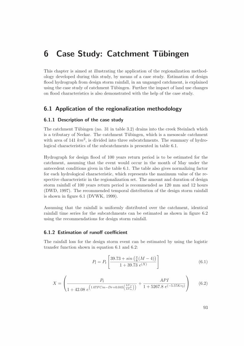
6 Case Study: Catchment Tubingen
This chapter is aimed at illustrating the application of the regionalization method-ology developed during this study, by means of a case study. Estimation of designflood hydrograph from design storm rainfall, in an ungauged catchment, is explainedusing the case study of catchment Tubingen. Further the impact of land use changeson flood characteristics is also demonstrated with the help of the case study.
6.1 Application of the regionalization methodology
6.1.1 Description of the case study
The catchment Tubingen (no. 31 in table 3.2) drains into the creek Steinlach whichis a tributary of Neckar. The catchment Tubingen, which is a mesoscale catchmentwith area of 141 km2, is divided into three subcatchments. The summary of hydro-logical characteristics of the subcatchments is presented in table 6.1.
Hydrograph for design flood of 100 years return period is to be estimated for thecatchment, assuming that the event would occur in the month of May under theantecedent conditions given in the table 6.1. The table also gives normalizing factorfor each hydrological characteristic, which represents the maximum value of the re-spective characteristic in the regionalization set. The amount and duration of designstorm rainfall of 100 years return period is recommended as 120 mm and 12 hours(DWD, 1997). The recommended temporal distribution of the design storm rainfallis shown in figure 6.1 (DVWK, 1999).
Assuming that the rainfall is uniformly distributed over the catchment, identicalrainfall time series for the subcatchments can be estimated as shown in figure 6.2using the recommendations for design storm rainfall.
6.1.2 Estimation of runoff coefficient
The rainfall loss for the design storm event can be estimated by using the logistictransfer function shown in equation 6.1 and 6.2:
Pl = Pt
[39.73 + sin
(π6 (M − 4)
)
1 + 39.73 e(X)
](6.1)
X =
Pt
1 + 42.08 e
(1.07FCm−Dr+0.045
(LUf
LUu
)) +API
1 + 5267.8 e(−5.57Kv2)
(6.2)
93

6 Case Study: Catchment Tubingen
Figure 6.1: Normalized temporal distribution of design storm rainfall (DVWK, 1999)
Figure 6.2: Rainfall time series
94

6.1 Application of the regionalization methodology
Table 6.1: Hydrological characteristics of the subcatchments (Tubingen)
HCs Subcatchments NormalizingA B C factor
M 5 5 5 11API 14.39 16.35 18.34 88.28Pt 120 120 120 82.31Tp 12 12 12 38.00A 40.38 36.08 64.56 73.88Per 58.38 48.24 55.26 73.08TC 1.92 2.02 1.67 3.20SL 0.06 0.11 0.15 0.35DR 1.24 1.06 1.04 1.77Kv2 0.61 0.49 0.71 0.98LUf 0.18 0.38 0.48 0.96LUu 0.13 0.12 0.09 0.21FC 2.76 1.52 1.59 3.92Qb 3.33 3.33 3.33 -
Using the equation 6.1 and 6.2 the hydrological characteristics, rainfall loss for sub-catchment A can be calculated as following:
X =
(120
1 + 42.08 e(1.07·2.76−1.24+0.045( 0.180.13))
+14.39
1 + 5267.8 e(−5.57·0.61)
)
= 0.56
hence,
Pl,A = 120
[39.73 + sin
(π6 (5 − 4)
)
1 + 39.73 e(0.56)
]
= 67.2 mm
Runoff coefficient (RC) for subcatchment A can be estimated as,
RCA = 1 − Pl
Pt
= 1 − 67.2
120= 0.44
Using iteration procedure to determine φ:φA = 5.6
95

6 Case Study: Catchment Tubingen
Similarly,for subcatchment B:RCB = 0.76φB = 2.4 mm
for subcatchment C:RCC = 0.74φC = 2.6 mm
Table 6.2 shows the effective rainfall time series for the subcatchments, calculatedusing the respective φ.
6.1.3 Estimation of Nash cascade parameters
The transfer functions derived to estimate Nash cascade parameters N and K inungauged catchment, using its hydrological characteristics, are as follows:
K = 7.14 T 0.7p TC0.22 e0.53LUu (6.3)
β = 5.62 T 0.37p SL−0.42 Per0.083 e0.18Pt (6.4)
N = β K−1.0 (6.5)
Before using in the transfer functions, the hydrological characteristics were normal-ized by the respective normalizing factors. Using the normalized hydrological char-acteristics in the equations 6.3 to 6.5, the Nash cascade parameters for subcatchmentA can be calculated as follows:
KA = 7.14 · 0.3160.7 · 0.60.22 · e0.53·0.606
= 3.95 hr
βA = 5.62 · 0.3160.37 · 0.171−0.42 · 0.80.083 · e0.18·1.45
= 9.68
NA = 9.68 · 3.95−1.0
= 2.45
Similarly,for subcatchment B:KB = 3.9 hrNB = 1.88
for subcatchment C:KC = 3.5 hrNC = 1.88
96

6.1 Application of the regionalization methodology
6.1.4 Estimation of flood hydrograph
Once the parameters N and K are estimated, the Nash cascade unit hydrograph andthe corresponding direct runoff hydrograph for a subcatchment ’j ’ can be derivedusing equation 6.6 and 6.7. Table 6.5 shows the ordinates of unit hydrographs andthe direct runoff hydrographs estimated for the subcatchments.
gi =1
K Γ(N)e−(
tiK
)
(tiK
)(N−1)
(6.6)
Qd(i,j) =i∑
l=1
Pe(i−l+1,j) Aj
3.6 Kj Γ(Nj)e−
(tl
Kj
) (tlKj
)(Nj−1)
(6.7)
The direct runoff hydrograph for a subcatchment can be routed to outlet of thecatchment using Muskingum routing procedure as explained in the subsection 2.3.2of chapter 2. Figure 6.3 shows the design flood runoff hydrograph at the outlet ofcatchment Tubingen, obtained after routing the direct runoff and adding the baseflow. The specific flood runoff volume (VQd), peak discharge (Qpeak) and time to itsarrival at outlet of the catchment (Tpeak), which are the essential characteristics fordesign and planning of flood protection schemes, are estimated from the design floodrunoff hydrograph as follows:
VQd = 79 mmQpeak = 257 m3/sTpeak = 9 hours
Table 6.2: Effective rainfall time series for the subcatchments (Tubingen)
Time SubcatchmentsA B C
1.0 1.1 4.3 4.02.0 1.1 4.3 4.03.0 1.1 4.3 4.04.0 8.4 11.6 11.45.0 19.4 22.6 22.46.0 19.4 22.6 22.47.0 0.4 3.6 3.48.0 0.4 3.6 3.49.0 0.4 3.6 3.410.0 0.4 3.6 3.411.0 0.4 3.6 3.412.0 0.4 3.6 3.4
The figure 6.3 also shows the flood hydrograph corresponding to rainfall durationsof 8 hours and 16 hours, for the same amount of rainfall. One may observe that the
97

6 Case Study: Catchment Tubingen
Figure 6.3: Design flood hydrographs for different rainfall durations (Tubingen)
same amount rainfall over shorter duration may produce steeper hydrograph withmuch higher and quicker peak, on the other hand the longer duration of the rainfallleads to reduced and delayed peak. However the derived regionalization methodologydoes not indicate the effect of rainfall duration on the flood runoff volume.
6.2 Assessment of impact of land use changes
Rapid land use changes, particularly deforestation due to ever increasing anthro-pogenic activities in the past few centuries, have reflected in severe impact on catch-ment and regional hydrology in various parts of the world. Of the most criticalfactors influenced by land use changes are the processes of runoff generation andrunoff propagation. Quantification of the impact of land use changes on the hydro-logical processes has been keenly pursued by hydrologist during the last decades.Harbor (1994) employed SCS curve number based distributed model for assessmentof long-term hydrological impact of land use changes. Wooldridge et. al. (2001) aswell as Hundecha and Bardossy (2004) associated the parameters of semi-distributedconceptual models with relative area of land use classes, thus, conveyed the impactof land use changes on the runoff response via model parameters. Samaniego (2003)carried out the assessment of hydrological consequences of different land use scenar-ios in meso-scale catchments by associating the critical runoff characteristics withphysiographical factors, which represent topography, morphology, climate and landuse of a catchment, through empirical models. The land use scenarios were predictedusing spatially distributed stochastic model. Several other region specific studies are
98
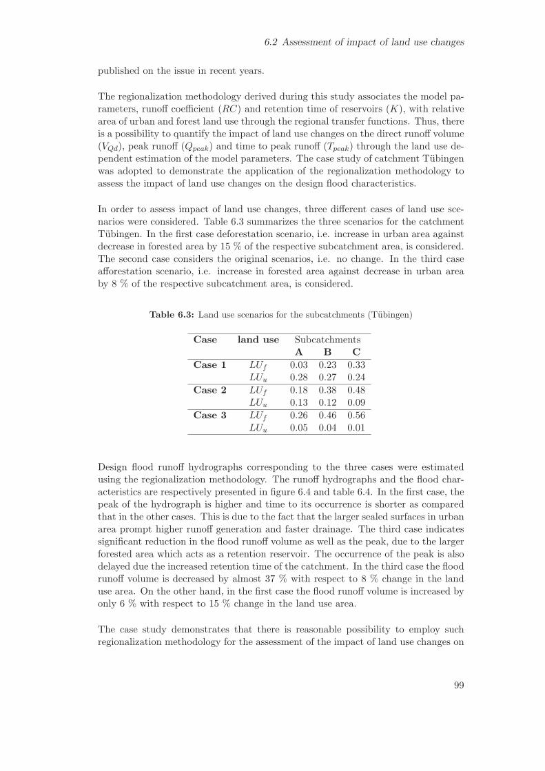
6.2 Assessment of impact of land use changes
published on the issue in recent years.
The regionalization methodology derived during this study associates the model pa-rameters, runoff coefficient (RC) and retention time of reservoirs (K), with relativearea of urban and forest land use through the regional transfer functions. Thus, thereis a possibility to quantify the impact of land use changes on the direct runoff volume(VQd), peak runoff (Qpeak) and time to peak runoff (Tpeak) through the land use de-pendent estimation of the model parameters. The case study of catchment Tubingenwas adopted to demonstrate the application of the regionalization methodology toassess the impact of land use changes on the design flood characteristics.
In order to assess impact of land use changes, three different cases of land use sce-narios were considered. Table 6.3 summarizes the three scenarios for the catchmentTubingen. In the first case deforestation scenario, i.e. increase in urban area againstdecrease in forested area by 15 % of the respective subcatchment area, is considered.The second case considers the original scenarios, i.e. no change. In the third caseafforestation scenario, i.e. increase in forested area against decrease in urban areaby 8 % of the respective subcatchment area, is considered.
Table 6.3: Land use scenarios for the subcatchments (Tubingen)
Case land use SubcatchmentsA B C
Case 1 LUf 0.03 0.23 0.33LUu 0.28 0.27 0.24
Case 2 LUf 0.18 0.38 0.48LUu 0.13 0.12 0.09
Case 3 LUf 0.26 0.46 0.56LUu 0.05 0.04 0.01
Design flood runoff hydrographs corresponding to the three cases were estimatedusing the regionalization methodology. The runoff hydrographs and the flood char-acteristics are respectively presented in figure 6.4 and table 6.4. In the first case, thepeak of the hydrograph is higher and time to its occurrence is shorter as comparedthat in the other cases. This is due to the fact that the larger sealed surfaces in urbanarea prompt higher runoff generation and faster drainage. The third case indicatessignificant reduction in the flood runoff volume as well as the peak, due to the largerforested area which acts as a retention reservoir. The occurrence of the peak is alsodelayed due the increased retention time of the catchment. In the third case the floodrunoff volume is decreased by almost 37 % with respect to 8 % change in the landuse area. On the other hand, in the first case the flood runoff volume is increased byonly 6 % with respect to 15 % change in the land use area.
The case study demonstrates that there is reasonable possibility to employ suchregionalization methodology for the assessment of the impact of land use changes on
99

6 Case Study: Catchment Tubingen
Table 6.4: Design flood characteristics corresponding to the land use scenarios
VQd Qpeak Tpeak
Case 1 83.9 262 7Case 2 79.0 257 9Case 3 50.3 191 10
Figure 6.4: Flood runoff hydrographs corresponding to the land use scenarios
the flood characteristics. However, the case study also reveals that the assessment forthe three land use scenarios, when compared to each other, seems to be inconsistent.The reason behind the inconsistency, can be explained as the lower sensitivity of thelogistic transfer function for rainfall loss to the smaller ratio between areas of forestand urban land use (
LUf
LUu).
100

6.2 Assessment of impact of land use changes
Table 6.5: Ordinates of unit hydrograph and direct runoff hydrograph for the subcatch-ments (Tubingen)
Time SubcatchmentsA B C
UH Q UH Q UH Q
1 0.021 0.2 0.063 2.7 0.074 5.42 0.044 0.8 0.090 6.6 0.103 12.83 0.062 1.5 0.099 10.8 0.110 20.84 0.073 4.1 0.099 19.7 0.107 38.35 0.078 11.2 0.093 37.2 0.098 73.56 0.079 22.7 0.084 58.0 0.087 114.67 0.077 32.8 0.075 67.4 0.075 130.68 0.072 39.7 0.065 70.8 0.063 134.29 0.067 43.5 0.056 70.8 0.053 131.110 0.060 44.7 0.047 68.9 0.044 124.711 0.054 44.1 0.040 65.9 0.036 116.912 0.047 42.2 0.033 62.6 0.029 108.813 0.041 39.5 0.028 56.9 0.023 96.714 0.036 36.1 0.023 50.4 0.019 83.615 0.031 32.5 0.019 43.8 0.015 70.916 0.026 28.9 0.015 37.5 0.012 59.217 0.022 25.4 0.013 31.8 0.010 48.918 0.019 22.1 0.010 26.8 0.008 40.119 0.016 19.1 0.008 22.3 0.006 32.620 0.013 16.4 0.007 18.5 0.005 26.321 0.011 13.9 0.005 15.3 0.004 21.122 0.009 11.8 0.004 12.6 0.003 16.923 0.008 9.9 0.004 10.3 0.002 13.424 0.006 8.3 0.003 8.4 0.002 10.725 0.005 7.0 0.002 6.8 0.001 8.426 0.004 5.8 0.002 5.5 0.001 6.727 0.003 4.8 0.001 4.5 0.001 5.228 0.003 4.0 0.001 3.6 0.001 4.129 0.002 3.3 0.001 2.9 0.001 3.230 0.002 2.7 0.001 2.3 0.000 2.5
101

7 Summary and Outlook
7.1 Summary
Although several regionalization methodologies have been proposed for hydrologicalpredictions in ungauged catchments, only few of them are based on physically rea-sonable approaches. Most of the existing methodologies employ a purely data drivenregression approach to derive regional transfer functions which associate model pa-rameters with hydrological characteristics. While doing so, the physical implicationsof the derived relationships, with respect to underlying rainfall-runoff processes, areusually disregarded. The purely data driven approach may lead to an excellent good-ness fit performance during regression, however, the derived transfer functions maynot represent physically reasonable relationships. A transfer function with no phys-ical basis may exhibit excellent goodness fit during regression, however, can lead towholly fallacious, if not unrealistic, predictions for an event beyond the data set usedfor the regression. Such transfer functions often lack the robustness and transferabil-ity to produce reliable predictions in ungauged catchments.
The conventional approaches employ a two step procedure to establish transfer func-tions: separate calibration of model parameters for each of the gauged catchments,then derivation of the transfer function which associates a parameter with hydrolog-ical characteristics through a regression procedure. However, due to inter-parameterinteraction, calibration often leads to several equally good parameters, not each ofthem may fit into a unique transfer function. Thus, the derivation of transfer func-tions through the two step regionalization procedure is subjected to the parameteridentification problem. This often leads to weak regional transfer functions. Finally,parameter sets calibrated at catchment scale often do not correspond to optimumparameter set at regional scale. To obtain an efficient and robust regionalizationmethodology, it must be developed for optimum regional performance instead ofcatchment specific performance.
The main goal of this study was to develop a robust, physically reasonable and prac-tically simple regionalization methodology for predictions of flood runoff volume,peak runoff and time to peak runoff, in ungauged catchments. Instead of developingcatchment specific solutions, the study was aimed at a general methodology for re-gional solutions. To keep the methodology practically simple, a parsimonious eventbased Nash cascade conceptual model was adopted. The model uses three parame-ters: runoff coefficient (RC), number of reservoirs (N) and reservoir constant (K).Transfer functions to estimate the model parameters in ungauged catchments, usingreadily available hydrological characteristics, were derived for the study area underconsideration. The study was essentially focused on deriving the transfer functionswhich are based on physically reasonable relationships. To ensure the optimum re-
102

7.1 Summary
gional solution, the transfer functions were optimized for aggregated regional modelperformance.
If total rainfall (Pt) and rainfall loss (Pl) occurred during a rainfall-runoff event areknown, RC for the event can be estimated. Therefore, a transfer function for Pl,instead of for RC, was derived during this study. Four different approaches were em-ployed to derive four different transfer functions for Pl. Three of them were purelydata driven approaches, based on multiple linear regression (MLTF), artificial neuralnetwork (ANNTF) and fuzzy logic (FLTF). The fourth approach was a data-plus-knowledge driven approach based on logistic regression (LoTF). All the approacheslead to highly acceptable goodness fit between observed and calculated Pl, especially,ANNTF, FLTF and LoTF yield excellent goodness fit primarily due to their highflexibility.
However, the validation for physical processes reveals that the purely data drivenapproaches fail to capture the physical relationships pertaining to rainfall loss pro-cesses. The comparison of the signs of derivatives of the functional relationships withthat of the physical relationships between Pl and the predictors reveals that, for anindividual event, the response of ANNTF and FLTF to hydrological changes oftenconflicts with the response anticipated from the a priori knowledge of rainfall lossprecesses.
Conceptual and empirical functions are extensively implemented for predicting vari-ous hydrological responses mainly, to address the lack of sufficient hydrological dataand understanding of the physical processes. Usually, they are not based on detaileddescriptions of the physical processes. However, it is crucial that the conceptual andempirical functions provide not only good “curve fitting” tools but also “correct”representations of the known rainfall-runoff processes. Due to their excessive free-dom, ANNTF and FLTF lead to extremely flexible, non linear transfer functionswhich perform excellent in terms of goodness fit. However, they fail to capture anyphysical relationship pertaining to rainfall loss processes, and thus do not lead tophysically reasonable transfer functions. Hence, application of these approaches forextrapolation (or regionalization), to predict a response beyond the range of thedataset used their derivation, is highly questionable. MLTF exhibits physically rea-sonable relationships except for the predictor “month”, however, it cannot capturethe non-linearities of the relationships.
A highly flexible transfer function without an appropriate physical basis may lead toa disastrous anomaly between predicted response and the response of rainfall-runoffprocesses in nature, and consequently, to highly uncertain predictions. The fuzzylogic approach is transparent and easy to incorporate a priori knowledge of rainfall-runoff processes in the form of fuzzy rules. But, in the case of artificial neural network(ANN), due to its opaque structure, it is extremely difficult to analyze the functionalrelationships and to incorporate a priori knowledge. Thus, the purely data drivenapproaches, such as ANN, limit themselves merely to black box approaches whosepredictive uncertainty is difficult, if not impossible to analyze.
103

7 Summary and Outlook
In the case of LoTF, the a priori knowledge of the physical relationships between Pl
and the predictors was embedded into the transfer function. The validation of LoTFfor the physical relationships confirms that LoTF represents physically reasonablerelationships. The validation of LoTF for spatial transferability, for the catchmentswhich were not used for its derivation, suggests that the transfer function is effi-cient at estimating Pl and, subsequently, RC in ungauged catchments. Being basedon physically reasonable relationships and flexible enough to replicate non-linear re-lationships, LoTF makes the most suitable transfer function to estimate Pl in theungauged catchments in the study area under consideration.
Due to strong inter-parameter interaction between Nash cascade parameters N andK, separate regionalization of the parameters was not viable. The initial attemptto derive the inter-parameter function led to the revelation that the parameterscan be related to each through a power function, and further, the coefficient (β) ofthe power function can be attributed to hydrological characteristics. Therefore, thetransfer functions were derived for the parameter K and the coefficient β. Thus, Kand β can be estimated from hydrological characteristics and N can be estimatedusing the inter-parameter function. The approach addresses the problem of param-eter identification by regionalizing the inter-parameter relationship itself. To obtainoptimum regional transfer functions, the transfer functions were optimized at oncefor the whole set of gauged catchments, using mean Nash-Sutcliffe coefficient as anaggregated regional objective function. The optimization leads to fairly high regionalperformance as well as goodness fit of peak runoff and time to peak runoff. The op-timized transfer function for K associates the parameter with time of concentration,duration of rainfall and relative area of urban land use. The transfer function for βassociates the coefficient with duration of rainfall, total rainfall, slope and perimeter.Both transfer functions were formed using a combination of power and exponentialfunctions.
Since Nash cascade parameters are conceptual, their physical relationship with hydro-logical characteristics can not be identified and embedded into the transfer functions.However, the physical relationships between the catchment characteristics, used inthe transfer functions, and shape of unit hydrograph can be derived from the apriori knowledge of runoff propagation processes. Therefore, the transfer functionswere validated for their response, in terms of shape of modeled unit hydrograph,to changes in the catchment characteristics. The validation led to the conclusionthat the derived transfer functions captures the physical relationships between thecatchment characteristics and shape of unit hydrograph, thus, can be regarded asphysically reasonable. The validation for spatial transferability indicates that thetransfer functions leads to robust and highly efficient performance, in terms of good-ness fit of runoff hydrograph, peak runoff, and time to peak runoff in the catchmentswhich are not used for the optimization.
Analysis of performance of the derived regionalization methodology, for individualevents, reveals that the methodology performs poorly for small rainfall events. Thisleads to the conclusion that the methodology may not be valid for the small rainfallevents which are below certain threshold of amount (< 20 mm) and duration (10 hr)
104

7.1 Summary
of rainfall. The performance of the methodology might also be hindered due to inad-equate estimation of rainfall input. The performance in the catchments at foothillsof Swabian Alps is also poor. This was expected due to the presence of the karsticaquifers which lead to the dominance of subsurface drainage.
The derived regionalization methodology uses readily available hydrological char-acteristics and parsimonious modeling as well as transfer function approach. Itis based on physically reasonable relationships, thus, “appropriately” representsrainfall-runoff processes. The methodology reasonably handles the problem of pa-rameter identification by regionalizing the inter-parameter relationship, additionally,it is optimized for the regional performance. Therefore, the derived regionaliza-tion methodology, although it may not offer the best catchment specific solution, isa practical, robust and efficient regional approach to reliable predictions of designflood characteristics in ungauged catchments in the region.
To examine its utility, the derived regionalization methodology was compared withSCS curve number method and the Lutz procedure, which are the widely used stan-dard practices for flood predictions in ungauged catchments. The comparisons revealthat the derived regionalization methodology performs better than those standardpractices, at least for the region under consideration. This also implies that thederived methodology is practically useful and can be adopted into practice beyondits academic purpose. The case study of catchment Tubingen demonstrates the ap-plication of the methodology to estimate design flood characteristics in an ungaugedcatchment.
In case of continuous simulations, in order to adapt to event specific conditions, acontinuous model must be run for at least a complete hydrological cycle prior to anevent. But the derived regionalization methodology estimates the model parametersusing, not only the catchment characteristics, but also the event specific characteris-tics. Thus, the regionalization methodology adapts the event based model to eventspecific hydrological conditions without having it to run for long duration. Since theregionalization methodology also utilizes relative area of urban and forest land use,it may be used for predictions under changing land use conditions. The possibility ofusing the regionalization methodology for assessment of impact of land use changeson flood runoff characteristics was investigated through the case study of catchmentTubingen. Although the case study demonstrates a reasonable possibility of usingthe methodology for such assessment, the conclusion can be made that the derivedtransfer functions are inconsistent in reproducing impact of land use changes due tothe lack of “enough sensitivity” to the changes.
Finally, it must be mentioned that the approach employed during this study is generaland may be transferable to other “similar” regions. However the transfer functionsderived during the study are specifically for the study area under consideration andmay not be directly transfered to other regions.
105

7 Summary and Outlook
7.2 Outlook
Based on the observations and the experiences gained during the course of this study,following suggestions may be pointed out for the further possible studies in the similardirection:
• Due to inadequate quality of hourly rainfall data, daily rainfall data was disinte-grated into hourly scale using the available hourly data. This led to satisfactoryrainfall estimations, however, not essentially reliable. Further improvement inthe rainfall estimations, e.g. using radar measurements, may lead to significantincrease in the performance of the methodology.
• Due to lack of necessary data, soil classes based on hydraulic conductivity wereused during the study. However, the soil classes may not properly representthe effect of the soil property on runoff generation. For the future study, ifpossible, use of mean hydraulic conductivity of subcatchment is recommended.
• During this study, investigation for the homogeneity of the region was notconducted, it was assumed to be fairly homogeneous. However, it may beworthwhile to carry out catchment classification based on hydrological homo-geneity, such classification may further improve the performance. The derivedregionalization methodology itself can be used for the catchment classification.The coefficients of the transfer functions can be calibrated separately for eachcatchment in the region using a same synthetic rainfall-runoff event. The catch-ments which yield similar coefficients of the transfer functions can be regardedas relatively homogeneous catchments.
• There is a possibility to use the derived regionalization methodology for as-sessment of impact of land use changes on flood characteristics. However therole of land use in the transfer functions must be reinvestigated. The poten-tial improvement in the assessment of the impact of land use changes lays inconsideration of seasonal land use management and using distributed modelingapproach designed to estimate the impact at smaller scales of 5 km2 to 10 km2.
• During the optimization of the transfer functions for Nash cascade parame-ters, the uncertainty due to equifinality was reduced by restricting the param-eter space through simplified inter-parameter relationship and the hydrologicalcharacteristics. However, it will be worthwhile to investigate the uncertaintyrelated to the simplification of the inter-parameter relationship. Furthermore,since runoff response of a catchment is highly influenced by spatial rainfall dis-tribution, the assessment of the uncertainty related to the estimation of spatialrainfall distribution is also recommended.
• The examples of purely data driven and data-plus-knowledge driven approachesunderline the significance of incorporating a priori knowledge of physical pro-cesses into a model. ANN and fuzzy logic approaches have shown signs ofgreat potential as futuristic tools for hydrological predictions, but their exces-sive flexibility must be restricted by using the available knowledge of underlyingphysical processes.
106

References
Abbott et. al., 1986: Abbott, M. B., Bathurst, J. C., Cunge, J. A., O’Connell,P. E. and Rasmussen, J., 1986. An Introduction to the European System: SystemeHydrologique Europeen (SHE), Journal of Hydrology, Vol. 87, 45-77.
Abdulla and Lettenmaier, 1997: Abdulla, F. A. and Lettenmaier, D. P., 1997.Development of Regional Parameter Estimation Equations for a Macroscale Hydro-logic Model, Journal of Hydrology, Vol. 197(1), 230-257.
Ahmed and de Marsily, 1987: Ahmed, S. and de Marsily, G., 1987. Comparisonof Geostatistical Methods for Estimating Transmissivity Using Data on Transmissiv-ity and Specific Capacity, Water Resources Research, Vol. 23.
Ahmed and Marsily, 1987: Ahmed, S., and Marsily, G., 1987. Comparison ofGeostatistical Methods for Estimating Transmissivity Using Data on Transmissivityand Specific Capacity, Water Resources Research, 23(9), 1717-1737.
Andrade, 1999: Andrade, E. M., 1999. Regionalization of Small Watersheds inArid and Semi-arid Regions: Cluster and Andrew’s Curve Approaches, EngenhariaAgrıcola, Vol. 18(4).
Ashkar and Mahdi, 2003: Ashkar, F. and Mahdi, S., 2003. Comparison of TwoFitting Methods for the Log-logistic Distribution, Water Resources Research, Vol.39(8), 1217.
Augustin et. al., 2001: Augustin, N., Cummins, R. and French, D., 2001. Explor-ing Spatial Vegetation Dynamics Using Logistic Regression and a Multinomial LogitModel, Journal of Applied Ecology, Vol. 38, 991-1006.
Bardossy and Duckstein, 1994: Bardossy, A. and Duckstein, L., 1994. FuzzyRule-Based Modeling with Applications to Geophysical, Biological and EngineeringSystems, CRC Press, Boca Raton.
Bardossy et. al., 1999: Bardossy, A., Hartmann, G. and Giese, H., 1999. Impactof Climate Change on River Basin Hydrology under Different Climatic Conditions,Final Report CC-HYDRO.
Bardossy, 2000: Bardossy, A., 2000. Compendium of Hydrology, Institute of Hy-draulic Engineering, Universitaet Stuttgart.
Bardossy et. al., 2003: Bardossy, A., Haberlandt, U. and Krysanova, V., 2003.
107

References
Automatic Fuzzy-Rule Assessment and Its Application to the Modeling of NitrogenLeaching for Large Regions, Soft Computing, Vol. 7, 370-385.
Bardossy et. al., 2006: Bardossy, A., Mascellani, G. and Franchini, M., 2006.Fuzzy Unit Hydrograph, Water Resources Research, Vol. 42(2), 1-17.
Bardossy, 2007: Bardossy, A., 2007. Calibration of Hydrological Model Parametersfor Ungauged Catchments, Hydrology and Earth System Sciences, Vol. 11, 703710.
Bergstrom, 1995: Bergstrom, S., 1995. The HBV model, in Computer Models ofWatershed Hydrology by Singh, V. P., Water Resources Publications.
Beven and Kirkby, 1979: Beven, K. J. and Kirkby, M. J., 1979. A Physically-Based Variable Contributing Area Model of Basin Hydrology, Hydrological, SciencesBulletin, Vol. 24, 43-69.
Beven and Freer, 2001: Beven, K. and Freer, J., 2001. Equifinality, Data As-similation, and Data Uncertainty Estimation in Mechanistic Modelling of ComplexEnvironmental Systems Using the GLUE Methodology, Journal of Hydrology, Vol.249, 1129.
Beven et. al., 1987: Beven, K., Calver, A. and Morris, E. M., 1987. The Instituteof Hydrology Distributed Model, Institute of Hydrology Report No. 98, Wallingford,U.K.
Beven, 2000: Beven, k. J., 2000. Uniqueness of Place and Process Representationsin Hydrological Modelling, Hydrology and Earth System Sciences, Vol. 4(2).
Beven, 2001: Beven, K. J., 2001. Rainfall Runoff Modelling, John Wiley Sons, Ltd.
Bhaskar et. al., 1989: Bhaskar, N. R., O’Connor, C. A., Myers, H. A. and Puck-ett, W. P., 1989. Regionalization of Flood Data Using Probability Distributions andTheir Parameters, National Technical Information Service, Springfield VA 22161 asPB90-159252/AS.
Bloeschl, 2005: Bloeschl, G., 2005. Rainfall-Runoff Modeling of Ungauged Catch-ments, Encyclopedia of Hydrological Sciences, edited by Anderson, M. G., JohnWiley Sons, Ltd.
Bocchiola et. al., 2003: Bocchiola, D., Michele, C. D. and Rosso, R., 2003. Reviewof Recent Advances in Index Flood Estimation, Hydrological Earth System Sciences,Vol. 7(3), 283-296.
Boughton et. al., 1999: Boughton, W. C., Muncaster, S. H., Srikanthan, R.,Weinmann, P. E. and Mein, R. G., 1999. Continuous Simulation for Design FloodEstimation - A Workable Approach, Water 99 Joint Congress, Brisbane, Institution
108

References
of Engineers, Australia, 178 -183.
Bremicker, 2000: Bremicker, M., 2000. Das Wasserhaushaltsmodell LARSIM -Modellgrundlagen und Anwendungsbeispiele, Freiburger Schriften zur Hydrologie, In-stitut fur Hydrologie, University of Freiburg, Vol. 11.
Bronstert et. al., 2002: Bronstert, A., Niehoff, D. and Burger, G., 2002. Effectsof Climate and Land Use Change on Storm Runoff Generation: Present Knowledgeand Modelling Capabilities, Hydrological Processes, Vol. 16(2), 509-529.
Burn and Boorman, 1993: Burn, D. H. and Boorman, B. D., 1993. Estimationof Hydrological Parameters at Ungauged Catchments, Journal of Hydrology, Vol. 143.
Charalambous, 2004: Charalambous, J., 2004. Application of Monte Carlo Sim-ulation Technique with URBS Runoff-Routing Model for design flood Estimation inLarge Catchments, University of Western Sydney, url: http://library.uws.edu.au/adt-NUWS/public/adt-NUWS20050520.153001.
Chow et. al., 1988: Chow, V. T., Maidment, D. R. and Mays, L. W., 1988. Ap-plied Hydrology, McGraw Hill Book Company.
Chow, 1988: Chow, V. T., 1988. Handbook of Applied Hydrology, McGraw-HillBook Company, 1964.
Clark, 1945: Clark, C. O., 1945. Storage and the Unit Hydrograph, Transactionsof the American Society of Civil Engineers, Vol. 110, 1419-1446.
Croke and Norton, 2004: Croke, B. F. W. and Norton, J. P., 2004. Region-alisation of Rainfall-Runoff Models, Pahl-Wostl, C., Schmidt, S., Rizzoli, A.E. andJakeman, A.J. (eds), Complexity and Integrated Resources Management, Transac-tions of the 2nd Biennial Meeting of the International Environmental Modelling andSoftware Society, iEMSs, Osnabruck, Vol. 2, 1201-1208.
Cunderlik and Burn, 2001: Cunderlik J. M. and Burn, D. H., 2001. The use offlood regime information in regional flood frequency analysis, Hydrological SciencesJournal,Vol. 47(1), 77-92.
Dartmouth Flood Observatory, 2004: Dartmouth Flood Observatory, 2004.Global Active Archive of Large Flood Events, url: http://www.dartmouth.edu/ floods.
Das, 2006: Das, T., 2006. The Impact of Spatial Variability of Precipitation on thePredictive Uncertainty of Hydrological Models, Mitteilungen, Institut fuer Wasser-bau, Universitaet Stuttgart, Vol. 154.
Dawson and Wilby, 2001: Dawson, C. W. and Wilby, R. L., 2001. Hydrologi-cal Modeling Using Artificial Neural Networks, Progress in Physical Geography, Vol.
109

References
25(1), 80-108.
Dooge, 1977: Dooge, J. C. I., 1977. Problems and Methods of Rainfall-RunoffModeling, Mathematical models for surface water hydrology, edited by Cirani, T. T.,Maione, U. and Wallis, J. R.,John Wiley and Sons, 70-101.
Dreyfus, 2005: Dreyfus, G., 2005. Neural Networks: Methodology and Applica-tions, Springer Publications.
Duan et. al., 2006: Duan, Q., Schaake, J., Andreassian, V., Franks, S., Gupta, H.V., Gusev, Y. M., Habets, F., Hall, A., Hay, L., Hogue, T. S., Huang, M., Leavesley,G., Liang, X., Nasonova, O. N., Noilhan, J., Oudin, L., Sorooshian, S., Wagener,T. and Wood, E. F., 2006. Model Parameter Estimation Experiment (MOPEX): AnOverview of Science Strategy and Major Results From the Second and Third Work-shops, Journal of Hydrology, Vol. 320(1-2), 3-17.
DVWK, 1999: Deutscher Verband fur Wasserwirtschaft und Kulturbau, 1999. Ein-satz von Niederschlag-Abfluss-Modellen zur Ermittlung von Hochwasserabfluessen,Hochwasserabfluesse, DVWK Schriften, Heft 124.
DWD, 1997: Deutsche Wetter Dienst, 1997. Starkniedershlagshoehen fuer die Bun-desrepublik Deutschland (KOSTRA), Selbstverlag des Duetschen Wetterdienstes, Of-fenbach am Main.
Eberle et. al., 2002: Eberle, M., Buiteveld, H., Beersma, J., Krahe, P. and Wilke,K., 2002. Estimation of Extreme Floods in the River Rhine Basin by CombiningPrecipitation-Runoff Modelling and a Rainfall Generator, Proceeding of InternationalConference of Flood Estimation, Switzerland, CHR Report II-17.
Fernandez et. al., 2000: Fernandez, W., Vogel, R. M. and Sankarasubramanian,A., 2000. Regional Calibration of a Watershed Model, Hydrological, Sciences Jour-nal, Vol. 45(5), 689-708.
Fiorentino and Versace, 1985: Fiorentino, M. and Versace, P., 1985. RegionalFlood Frequency Estimation Using the Two-Component Extreme Value Distribution,Hydrological Sciences, Vol. 30(1), 5164.
Franchini and Pacciani, 1991: Franchini, M. and Pacciani, M., 1991. Compar-ative Analysis of Several Conceptual Rainfall-Runoff Models, Journal of Hydrology,Vol. 122(7), 161219.
Fuller, 1914: Fuller, W. E., 1914. Flood Flows, Transactions of the American So-ciety of Civil Engineers, Vol. 77, 564-617.
Funke et. al., 1999: Funke, R., Schumann, A. H. and Schultz, G. A., 1999. Re-gionalization of Parameters in Mesoscale Hydrological Models, IAHS Publication,Vol. 254, 171-179.
110

References
Gill, 1978: Gill, M. A., 1978. Flood Routing by the Muskingum Method Journal ofHydrology, Vol. 36, 353363.
Gupta and Sorooshian, 1983: Gupta, V. K. and Sorooshian, S., 1983. TheCalibration of Conceptual Catchment Models using Derivative-Based OptimizationAlgorithms. Water Resources Research, Vol. 19, 269276.
Goppert et. al., 1998: Goppert, H., lhringer, J., Plate, E. J. and Morgenschweis,G., 1998. Flood Forecasting Model for Improved Reservoir Management in the LenneRiver Catchment, Germany, Hydrological Sciences Journal. Vol. 43(2), 215-242.
Haan et. al., 1994: Haan, C. T., Barfield, B. J. and Hayes, J. C., 1994. DesignHydrology and Sedimentology for Small Catchments, Academic Press.
Haberlandt et. al., 2001: Haberlandt, U., Klocking, B., Krysanova, V. andBecker, A., 2001. Regionalisation of the Base Flow Index from Dynamically Simu-lated Flow Components - A Case Study in the Elbe River Basin, Journal of Hydrology,Vol. 248(1).
Hagan and Menhaj, 1994: Hagan, M. and Menhaj, M., 1994. Training Feed-forward Networks with the Marquardt Algorithm, IEEE Transactions on Neural Net-works, Vol. 5(6), 989-993.
Harbor, 1994: Harbor, J. M., 1994. A Practical Method for Estimating the Impactof Land Use Change on Surface Runoff, Groundwater Recharge and Wetland Hydrol-ogy, Journal of the American Planning Association, Vol. 60 (1), 91-104.
Hashemi et. al., 2000: Hashemi, A. M., Franchini, M., O’Connell and P. E., 2000.Climatic and Basin Factors Affecting the Flood Frequency Curve: PART I - A Sim-ple Sensitivity Analysis Based on the Continuous Simulation Approach, Hydrologyand Earth System Sciences, Vol. 4(3), 463-482.
Hazen, 1914: Hazen, A., 1914. Storage to be Provided in Impounding Reservoirs forMunicipal Water Supply, Transactions of the American Society of Civil Engineers,Vol. 77, 15391640.
Heuvelmans et. al., 2004: Heuvelmans, G., Muys, B. and Feyen, J., 2004. Anal-ysis of the Spatial Variation in the Parameters of the SWAT Model with Applicationin Flanders, Northern Belgium, Hydrology and Earth System Sciences, Vol. 8(5).
Hill and Mein, 1996: Hill, P. I. and Mein, R. G., 1996. Incompatibilities betweenStorm Temporal Patterns and Losses for Design Flood Estimation, Hydrology andWater Resources Symposium, Hobart, Tasmania, Vol. 2, 445-451.
Hipel, 1995: Hipel, K. W., 1995. Stochastic and Statistical Methods in Hydrologyand Environmental Engineering, Stochastic Environmental Research and Risk As-
111
References
sessment, Vol. 9(1), 1-11.
Holder, 1985: Holder, R. L., 1985. Multiple Regression in Hydrology, the Instituteof Hydrology, Wallingford, UK, ISBN 094 854000 1.
Horton, 1945: Horton, R. E., 1945. Erosional Development of Streams and TheirDrainage Basins: Hydrophysical Approach to Quantitative Morphology, Bulletin ofthe Geological Society of America, Vol. 56, 275370.
Hosmer and Lemeshow, 2000: Hosmer, D. W. and Lemeshow, S., 2000. AppliedLogistic Regression, Wiley Series in Probability and Statistics, John Wiley and Sons.
Hsu et. al., 1995: Hsu, K., Sorooshian, S. and Gupta, H., 1995. Artificial NeuralNetwork Modeling of the Rainfall-Runoff Process, Water Resources Research, Vol.31(10), 2517-2530.
Hydrocomp, 2002: Hydrocomp, Inc., 2002. Hydrologic Simulation Models: AnOverview, url: http://www.hydrocomp.com
Hundecha et. al., 2001: Hundecha, Y., Bardossy, A. and Theisen, H. W., 2001.Development of a Fuzzy Logic based Rainfall-runoff Model, Hydrological SciencesJournal, Vol. 46(3), 363377.
Hundecha and Bardossy, 2004: Hundecha, Y. and Bardossy, A., 2004. Model-ing of the Effect of Land Use Changes on the Runoff Generation of a River Basinthrough Parameter Regionalization of a Watershed Model, Journal of Hydrology, Vol.292(1/4), 281-295.
Jakeman et. al., 1990: Jakeman, A. J., Littlewood, I. G. and Whitehead, P. G.,1990. Computation of the Instantaneous Unit Hydrograph and Identifiable Compo-nent Flows with Application to Two Small Upland Catchments, Journal of Hydrology,Vol. 117, 275-300.
Jakeman et. al., 1992: Jakeman, A., Hornberger, G., Littlewood, I., Whitehead,P., Harvey, J. and Bencala, K. A, 1992. Systematic Approach to Modelling the Dy-namic Linkage of Climate, Physical Catchment Descriptors and Hydrologic ResponseComponents, Mathematics and Computers in Simulation, Vol. 33(5-6), 359-366.
Johnson and Wichern, 1992: Johnson, R. A. and Wichern, D. W., 1992. AppliedMultivariate Statistical Analysis, Prentice-Hall Inc., New Jersey.
Kirkpatrick et. al., 1983: Kirkpatrick, S., Gelatt, C. D. and Vecchi, M. P., 1983.Optimization by Simulated Annealing, Science, Vol. 220(4598), 671-679.
Kirpich, 1940: Kirpich, Z. P., 1940. Time of Concentration of Small AgriculturalWatersheds, Civil Engineering (N.Y.), Vol. 10(6), 362.
112

References
Klemes, 2000: Klemes, V., 2000. Tall Tells about Tails of Hydrological Distribu-tions. I, Journal of Hydrologic Engineering, Vol. 5(3), 227-231.
Kokkonen et. al., 2003: Kokkonen, T. S., Jakeman, A. J., Young, P. C. andKoivusalo, H. J., 2003. Predicting Daily Flows in Ungauged Catchments: ModelRegionalization from Catchment Descriptors at the Coweeta Hydrologic Laboratory,North Carolina, Hydrological Processes, Vol. 17(11).
Kokkonen, 2003: Kokkonen, T., 2003. Rainfall-Runoff Modeling -Comparisonof Modeling Strategies with Focun on Ungauged Predictions and Model Integration,Helsinki University of Technology Water Resources Publications, Espoo 2003, TKK-VTR-9.
Kottegoda and Rosso, 1997: Kottegoda, N. and Rosso, R., 1997. Statistics,Probability and Reliability for Civil and Environmental Engineers, McGraw Hill Pub-lications, New York, USA.
Kumar and Chatterjee, 2005: Kumar, R. and Chatterjee, C., 2005. RegionalFlood Frequency Analysis using L-Moments for North Brahmaputra Region of India,Journal of Hydrologic Engineering, Vol. 10(1), 1-7.
Kumar, et. al., 2002: Kumar, M., Raghuwanshi, N. S., Singh, R., Wallender, W.W. and Pruitt, W. O., 2002. Estimating Evapotranspiration Using Artificial NeuralNetwork, Journal of Irrigation and Drainage Engineering, Vol. 128(4), 224-233.
Lange, 1999: Lange, N. T., 1999. New Mathematical Approaches in HydrologicalModeling-An Application of Artificial Neural Networks, Physics and Chemistry ofthe Earth, Vol. 24(1-2), 3135.
Leavesley and Stannard, 1995: Leavesley, G. H. and Stannard, L. G., 1995.The Precipitation-Runoff Modeling System PRMS, Computer Models of WatershedHydrology, edited by Singh, V. P., Water Resources Publications, Highlands Ranch,281310.
Lee et. al., 2005: Lee, H., McIntyre, N. R., Wheater, H. S. and Young, A. R., 2005.Predicting Runoff in Ungauged UK Catchments, ICE Proceedings, Water Manage-ment, Vol. 159(2), 129-138.
Lutz, 1984: Lutz, W., 1984. Bereschnung von Hochwasserabfluessen unter An-wendung von Gebietskenngroessen, Institut fuer Hydrologie und Wasserwirtschaft,Universitaet karlsruhe, Heft 24.
Maidment, 1992: Maidment, D. R., 1992. Handbook of Hydrology, McGraw HillBook Co.
Manley, 1978: Manley, R. E., 1978. Simulation of Flows in Ungauged Basins,Hydrological Scineces Bulletin, Vol. 23(1).
113

References
McIntyre et. al., 2005: McIntyre, N., Lee, H., Wheater, H., Young, A. and Wa-gener, T., 2005. Ensemble Predictions of Runoff in Ungauged Catchments, WaterResources Research, Vol. 41, 1-14.
Merz and Bloeschl, 2004: Merz, R. and Bloeschl, G., 2004. Regionalisation ofCatchment Model Parameters, Journal of Hydrology, Vol. 287.
Michele and Rosso, 2001: Michele, C. and Rosso, R., 2001. Uncertainty Assess-ment of Regionalized Flood Frequency Estimates, Journal of Hydrologic Engineering,Vol. 6(6), 453-459.
Mockus, 1957: Mockus, V., 1957. Use of Storm and Watershed Characteristics inSynthetic Hydrograph Analysis and Application American Geophysical Union, South-west Region Meeting, Sacramento, California.
Moore et. al., 1991: Moore, I. D., Grayson, R. B. and Ladson, A. R., 1991. Dig-ital Terrain Modelling -A Review of Hydrological, Geomorphological and BiologicalApplications, Hydrological Processes, Vol. 5, 3-30.
Morel-Seytoux and Verdin, 1981: Morel-Seytoux, H. J. and Verdin, J. P., 1981.Extension of the Soil Conservation Service Rainfall-runoff Methodology for UngagedWatersheds., Federal Highway Administration, Report no. FHWA/RD-81/060.
Mulvany, 1851: Mulvany, T. J., 1851. On the Use of Self-registering Rain andFlood Gauges in Making Observations of the Rainfall and Flood Discharges in aGiven Catchment, Transactions and Minutes of the Proceeding of the Institute ofCivil Engineers of Ireland, Session 1850-1, v.IV, pt. II, Dublin, Ireland.
Nash, 1957: Nash, J. E., 1957. The Form of the Instantaneous Unit Hydrograph,General Assembly of Toronto, IASH Publications, Vol. 3(45), 114119.
Nash, 1960: Nash, J. E., 1960. A Unit Hydrograph Study with Particular Referenceto British Catchments, Proceedings: Institute of Civil Engineering, London, Vol. 17.
Nash and Sutcliffe, 1970: Nash, J. E. and Sutcliffe, J. V., 1970. River Now Fore-casting through Conceptual Models I: discussion of principles, Journal of Hydrology,Vol. 10, 282-290.
NERC, 1975: NERC, 1975. Flood Studies Report, Natural Environment ResearchCouncil, UK, Hydrological Studies, Vol. 1.
NRCS, 2004: Natural Resources Conservation Service, 2004. National EngineeringHandbook, Part 630 Hydrology, US Department of Agriculture, Washington.
ODonnell, 1960: ODonnell, T., 1960. Instantaneous Unit Hydrograph Derivationby Harmonic Analysis, Proceedings of General Assembly Helsinki, IAHS Publica-
114

References
tions, Vol. 51, 546-557.
Onyando et. al., 2005: Onyando, J. O., Olang, L. O. and Chemelil, M. C., 2005,Regional Analysis of Conceptual Rainfall Runoff Models for Runoff Simulation InUngauged Catchments: The Case Of Upper Ewaso Ngiro Drainage Basin in Kenya,Journal of Civil Engineering Research and Practice, Vol. 2(1), 23-37.
Patil, 2004: Patil, S., 2004. Correlation between River Density and Baseflow Com-ponent, Masters Thesis, WAREM, Universitaet Stuttgart.
Perera, 1999: Perera, C., 1999. Testing of Recent Flood Estimation Inputs for Vic-torian Rural Ungauged Catchments, Proceedings from the Water 99 Joint Congress,Brisbane, Institution of Engineers, Australia, 649-654.
Pfister et. al., 2004: Pfister, L., Kwadijk, J., Musy, A., Bronstert, A. and Hoff-mann, L., 2004. Climate Change, Land Use Change and Runoff Prediction in theRhine-Meuse Basins, River Research and Applications, Vol. 20(3), 229-241.
Post et. al., 1998: Post, D. A., Jones, J. A. and Grant, G. E., 1998. An ImprovedMethodology for Predicting the Daily Hydrologic Response of Ungauged Catchments,Environmental Modelling Software, Vol. 13.
Post and Jakeman, 1999: Post, D. A. and Jakeman, A. J., 1999. Predictingthe Daily Streamflow of Ungauged Catchments in S.E. Australia by Regionalising theParameters of a Lumped Conceptual Rainfall-Runoff Model, Ecological Modelling,Vol. 123, 91104.
Press and Wilson, 1978: Press, S. J. and Wilson, S., 1978. Choosing BetweenLogistic Regression and Discriminant Analysis, Journal of the American StatisticalAssociation, Vol. 73(364), 699-705.
Rahman et. al., 2002: Rahman, A., Carroll, D. and Weinmann, E., 2002. In-tegration of Monte Carlo Simulation Technique with URBS Model for Design FloodEstimation, Proceedings of 27 National Hydrology and Water Resources Symposium,Melbourne, Institute of Engineers, Australia.
Raines and Valdes, 1993: Raines, T. H. and Valdes, J. B., 1993. Estimationof Flood Frequencies for Ungauged Catchments, Journal of Hydraulic Engineering,119(10), 11381154.
Rao and Srinivas, 2006: Rao, A. R. and Srinivas, V. V., 2006. Regionalization ofWatersheds by Fuzzy Cluster Analysis, Journal of Hydrology, Vol. 318, 5779.
Rao, 2000: Rao, A. R., 2000. Flood Frequency Analysis, CRC Press, USA.
Reynard et. al., 2001: Reynard, N. S., Prudhomme, C. and Crooks, S. M., 2001.The Flood Characteristics of Large U.K. Rivers: Potential Effects of Changing Cli-
115
References
mate and Land Use, Climatic Change, Springer Netherlands, Vol. 48(2/3), 343-359.
Riley et. al., 1999: Riley, S. J., DeGloria, S. D. and Elliot, R., 1999. A TerrainRuggedness Index That Quantifies Topographic Heterogeneity, Intermountain Jour-nal of Sciences. Vol. 5(14), 2327.
Rodriguez-Iturbe and Valdes, 1979: Rodriguez-Iturbe, I., Valdes, J. V., 1979.The Geomorphologic Structure of Hydrologic Response, Water Resources Research,15(6), Vol. 1409-1420.
Rubinstein and Kroese, 2007: Rubinstein, R. Y. and Kroese, D. P., 2007. Sim-ulation and the Monte Carlo Method, second edition, John Wiley and Son, New York.
Samaniego, 2003: Samaniego, L. E., 2003. Hydrological Consequences of LandUse/Cover and Climatic Changes in Mesoscale Catchments, Institut fur Wasserbau,Universitat Stuttgart, Heft 118.
Schreider et. al., 2002: Schreider, S. Y., Jakeman, A. J., Gallant, J., and Mer-ritt, W. S., 2002. Prediction of Monthly Discharge in Ungauged Catchments underAgricultural Land Use in the Upper Ping Basin, Northern Thailand, Mathematicsand Computers in Simulation, Vol. 59.
Schumann, 1993: Schumann, A. H., 1993. Development of Conceptual Semi-distributed Hydrological Models and Estimation of their Parameters with the Aid ofGIS, Hydrological Sciences Journal, Vol. 38(6), 519-528.
SCS, 1972: Soil Conservation Service, 1972. National Engineering Handbook, Sec-tion 4: Hydrology, US Department of Agriculture, Washington.
Sefton et. al., 1995: Sefton, C. E. M., Whitehead, P. G., Eatherall, A., Littlewood,I. G. and Jakeman, A. J., 1995. Dynamic Response Characteristics of the PlynlimonCatchments and Preliminary Analysis of Relationships to Physical Descriptors, En-vironmental Modelling Techniques and Applications, Vol. 6(5), 465 - 472.
Serrano et. al., 1985: Serrano, S. E., Whitley, H. R. and Irwin, R. W., 1985. Ef-fects of Agricultural Drainage on Stream Flow in the Middle Thames River, Ontario,1949-1980 Canadian Journal of Civil Engineering, Vol. 12, 875-885.
Sharpley and Williams, 1990: Sharpley, A. N. and Williams, J. R., 1990. EPICEro-sion/Productivity Impact Calculator: 1. Model Documentation, Technical BulletinNo. 1768, US Department of Agriculture, Washington.
Sherman, 1932: Sherman, L. K., 1932. Streamflow from Rainfall by the Unit-Graph Method, Engineering News-Record, Vol. 108, 501-505.
Shu and Burn, 2003: Shu, Ch. and Burn, D. H., 2003. Spatial Patterns of Homo-geneous Pooling Groups for Flood Frequency Analysis, Hydrological Sciences Journal,
116

References
Vol. 48(4).
Singh, 1995: Singh, V. P., 1995. Computer Models of Watershed Hydrology, WaterResources Publications.
Sivapalan et. al., 2003: Sivapalan, M., Takeuchi, K., Franks, S. W., Gupta, V.K., Karambiri, H., Lakshmi, V., Liang, X., McDonnell, J. J., Mendiondo, E. M.,O’Connell, P. E., Oki, T., Pomeroy, J. W., Schertzer, D., Uhlenbrook, S. and Zehe,E., 2003. IAHS Decade on Predictions in Ungauged Basins (PUB) 2003-2012, Shap-ing an Exciting Future for the Hydrological Sciences, Hydrological Sciences Journal,Vol. 48(6), 857880.
Sivapalan et. al., 1987: Sivapalan, M., Beven, K. J. and Wood, E. F., 1987.On Hydrologic Similarity. 2. A Scaled Model of Storm Runoff Production, WaterResources Research, Vol. 23(12), 22662278.
Sliverman, 1986: Sliverman, B. W., 1986. Density Estimation, Chapman and Hall.
Smith et. al., 1995: Smith, R. E., Goodrich, D. C., Woolhiser, D. A. and Unkrich,C. L., 1995. KINEROS A Kinematic Runoff and Erosion Model, Computer Mod-els of Watershed Hydrology, edited by Singh, V. P., Water Resources Publications,Colorado, 1130.
Stueber et. al., 2000: Stueber, M., Gemmar, P. and Greving, M., 2000. MachineSupported Development of Fuzzy-Flood Forecast Systems, Proceedings of EuropeanConference on Advances in Flood Research, Potsdam, Germany, Vol. 2(65), 504515.
Tewolde and Smithers, 2006: Tewolde, M. H. and Smithers, J. C., 2006. FloodRouting in Ungauged Catchments Using Muskingum Methods, Water SA, Vol. 32(3),379-388.
Tung, 1985: Tung, Y. K., 1985. River Flood Routing by Nonlinear MuskingumMethod, Journal of Hydraulic Engineering, Vol. 111(12), 1447-1460.
Tung et. al. 1997: Tung, Y. K., Yeh, K. C. and Yang J. C., Regionalizationof Unit Hydrograph Parameters 1. Comparison of Regression Analysis Techniques,Stochastic Hydrology and Hydraulics, Vol. 11, 145-171.
Uhlenbrook et. al., 2007: Uhlenbrook, S., Didszun, J., Tilch, N., Mcdonnell, J.and Mcguire, K., 2007. Breaking Up is Always Difficult Landscape Discretizationas a Process-Transfer Approach for Prediction in Ungauged Basins, Predictions inUngauged Basins: PUB Kick-off, IAHS Publications, 309, 102-109.
Vandewiele et. al., 1995: Vandewiele, G. L. and Elias, A., 1995. Monthly WaterBalance of Ungauged Catchments Obtained by Geographical Regionalization, Journalof Hydrology, Vol. 170.
117

References
Wagener et. al., 2002: Wagener, T., Lees, M. J. and Wheater and H. S., 2002. AToolkit for the Development and Application of Hydrological Models, MathematicalModels of Large Watershed Hydrology, edited by Singh, V. P. and Frevert, D. K.,Water Resources Publications, USA, 91-140.
Wagener et. al., 2004: Wagener, T., Wheater, H. S. and Gupta, H., 2004. Raifall-Runoff Modelling in Gauged and Ungauged Catchments, Imperial College Press.
Wagener et. al., 2006: Wagener, T., Wheater, H. S., Schaake, J.and Duan, Q.,2006. Parameter Estimation and Regionalization for Continuous Rainfall-RunoffModels Including Uncertainty, Journal of hydrology, Vol. 320(1-2), 132-154.
Williams et. al., 1983: Williams, J. R., Dyke, P. T. and Jones, C. A., 1983.EPIC: A Model for Assessing the Effects of Erosion on Soil Productivity, Analysis ofEcological Systems: State-of-the-Art in Ecological Modeling, edited by Laurenroth,W. K., Elsevier, Amsterdam, 553-572.
Wooldridge et. al., 2001: Wooldridge, S., Kalma, J. and Kuczera, G., 2001. Pa-rameterisation of a Simple Semidistributed Model for Assessing the Impact of Land-Use on Hydrologic Response, Journal of Hydrology, Vol. 254, 16-32.
Young, 2000: Young, A., 2000. Regionalizing a Daily Rainfall-Runoff Model withinthe United Kingdom, PhD Thesis, University of Southampton.
Zadeh, 1965: Zadeh, L. A., 1965. Fuzzy Sets, Information and Control, Vol. 12(2),338-353.
118

Curriculum Vitae Sachin Ramesh Patil [email protected]
06.12.1978
1984 – 1987
1987 – 1994
1994 – 1997
1997 – 2001
2001 – 2004
2004 – 2008
Born in Jalgaon, India
Primary school am Ravsaheb Rupchand Vidyalay, Jalgaon, India
Secondary school am Ravsaheb Rupchand Vidyalay, Jalgaon, India
Diploma – civil engineering, Govt. Polytechnic, Jalgaon, Board of Technical Education, Mumbai, India
Bachelor - civil engineering, Veermata Jijabai Technological Institute, University of Mumbai, India
Master of Science - WAREM “Water Resources Engineering and Management” Universität Stuttgart
Doctoral research candidate, Institute of Hydraulic Engineering, Universität Stuttgart

Institut für Wasserbau Universität Stuttgart
Pfaffenwaldring 61 70569 Stuttgart (Vaihingen) Telefon (0711) 685 - 64717/64749/64752/64679 Telefax (0711) 685 - 67020 o. 64746 o. 64681 E-Mail: [email protected] http://www.iws.uni-stuttgart.de
Direktoren Prof. Dr. rer. nat. Dr.-Ing. András Bárdossy Prof. Dr.-Ing. Rainer Helmig Prof. Dr.-Ing. Silke Wieprecht Vorstand (Stand 1.2.2008) Prof. Dr. rer. nat. Dr.-Ing. A. Bárdossy Prof. Dr.-Ing. R. Helmig Prof. Dr.-Ing. S. Wieprecht Prof. Dr.-Ing. habil. B. Westrich Jürgen Braun, PhD Dr.-Ing. H. Class Dr.-Ing. S. Hartmann Dr.-Ing. H.-P. Koschitzky PD Dr.-Ing. W. Marx Dr. rer. nat. J. Seidel Emeriti Prof. Dr.-Ing. habil. Dr.-Ing. E.h. Jürgen Giesecke Prof. Dr.h.c. Dr.-Ing. E.h. Helmut Kobus, PhD
Lehrstuhl für Wasserbau und Wassermengenwirtschaft Leiter: Prof. Dr.-Ing. Silke Wieprecht Stellv.: PD Dr.-Ing. Walter Marx, AOR Lehrstuhl für Hydromechanik und Hydrosystemmodellierung Leiter: Prof. Dr.-Ing. Rainer Helmig Stellv.: Dr.-Ing. Holger Class, AOR Lehrstuhl für Hydrologie und Geohydrologie Leiter: Prof. Dr. rer. nat. Dr.-Ing. András Bárdossy Stellv.: Dr. rer. nat. Jochen Seidel VEGAS, Versuchseinrichtung zur Grundwasser- und Altlastensanierung Leitung: Jürgen Braun, PhD Dr.-Ing. Hans-Peter Koschitzky, AD Versuchsanstalt für Wasserbau Leiter: apl. Prof. Dr.-Ing. habil. Bernhard Westrich
Verzeichnis der Mitteilungshefte
1 Röhnisch, Arthur: Die Bemühungen um eine Wasserbauliche Versuchsanstalt an
der Technischen Hochschule Stuttgart, und Fattah Abouleid, Abdel: Beitrag zur Berechnung einer in lockeren Sand geramm-ten, zweifach verankerten Spundwand, 1963
2 Marotz, Günter: Beitrag zur Frage der Standfestigkeit von dichten Asphaltbelägen
im Großwasserbau, 1964 3 Gurr, Siegfried: Beitrag zur Berechnung zusammengesetzter ebener Flächen-
tragwerke unter besonderer Berücksichtigung ebener Stauwände, mit Hilfe von Randwert- und Lastwertmatrizen, 1965
4 Plica, Peter: Ein Beitrag zur Anwendung von Schalenkonstruktionen im Stahlwas-
serbau, und Petrikat, Kurt: Möglichkeiten und Grenzen des wasserbaulichen Ver-suchswesens, 1966

2 Institut für Wasserbau * Universität Stuttgart * IWS
5 Plate, Erich: Beitrag zur Bestimmung der Windgeschwindigkeitsverteilung in der durch eine Wand gestörten bodennahen Luftschicht, und Röhnisch, Arthur; Marotz, Günter: Neue Baustoffe und Bauausführungen für den Schutz der Böschungen und der Sohle von Kanälen, Flüssen und Häfen; Geste-hungskosten und jeweilige Vorteile, sowie Unny, T.E.: Schwingungs-untersuchungen am Kegelstrahlschieber, 1967
6 Seiler, Erich: Die Ermittlung des Anlagenwertes der bundeseigenen Bin-
nenschiffahrtsstraßen und Talsperren und des Anteils der Binnenschiffahrt an die-sem Wert, 1967
7 Sonderheft anläßlich des 65. Geburtstages von Prof. Arthur Röhnisch mit Beiträ-
gen von Benk, Dieter; Breitling, J.; Gurr, Siegfried; Haberhauer, Robert; Hone-kamp, Hermann; Kuz, Klaus Dieter; Marotz, Günter; Mayer-Vorfelder, Hans-Jörg; Miller, Rudolf; Plate, Erich J.; Radomski, Helge; Schwarz, Helmut; Vollmer, Ernst; Wildenhahn, Eberhard; 1967
8 Jumikis, Alfred: Beitrag zur experimentellen Untersuchung des Wassernach-
schubs in einem gefrierenden Boden und die Beurteilung der Ergebnisse, 1968 9 Marotz, Günter: Technische Grundlagen einer Wasserspeicherung im natürlichen
Untergrund, 1968 10 Radomski, Helge: Untersuchungen über den Einfluß der Querschnittsform wellen-
förmiger Spundwände auf die statischen und rammtechnischen Eigenschaften, 1968
11 Schwarz, Helmut: Die Grenztragfähigkeit des Baugrundes bei Einwirkung vertikal
gezogener Ankerplatten als zweidimensionales Bruchproblem, 1969 12 Erbel, Klaus: Ein Beitrag zur Untersuchung der Metamorphose von Mittelgebirgs-
schneedecken unter besonderer Berücksichtigung eines Verfahrens zur Bestim-mung der thermischen Schneequalität, 1969
13 Westhaus, Karl-Heinz: Der Strukturwandel in der Binnenschiffahrt und sein Einfluß
auf den Ausbau der Binnenschiffskanäle, 1969 14 Mayer-Vorfelder, Hans-Jörg: Ein Beitrag zur Berechnung des Erdwiderstandes un-
ter Ansatz der logarithmischen Spirale als Gleitflächenfunktion, 1970 15 Schulz, Manfred: Berechnung des räumlichen Erddruckes auf die Wandung kreis-
zylindrischer Körper, 1970 16 Mobasseri, Manoutschehr: Die Rippenstützmauer. Konstruktion und Grenzen ihrer
Standsicherheit, 1970 17 Benk, Dieter: Ein Beitrag zum Betrieb und zur Bemessung von Hochwasser-
rückhaltebecken, 1970

Verzeichnis der Mitteilungshefte 3
18 Gàl, Attila: Bestimmung der mitschwingenden Wassermasse bei überströmten Fischbauchklappen mit kreiszylindrischem Staublech, 1971,
19 Kuz, Klaus Dieter: Ein Beitrag zur Frage des Einsetzens von Kavitationserschei-
nungen in einer Düsenströmung bei Berücksichtigung der im Wasser gelösten Gase, 1971,
20 Schaak, Hartmut: Verteilleitungen von Wasserkraftanlagen, 1971 21 Sonderheft zur Eröffnung der neuen Versuchsanstalt des Instituts für Wasserbau
der Universität Stuttgart mit Beiträgen von Brombach, Hansjörg; Dirksen, Wolfram; Gàl, Attila; Gerlach, Reinhard; Giesecke, Jürgen; Holthoff, Franz-Josef; Kuz, Klaus Dieter; Marotz, Günter; Minor, Hans-Erwin; Petrikat, Kurt; Röhnisch, Arthur; Rueff, Helge; Schwarz, Helmut; Vollmer, Ernst; Wildenhahn, Eberhard; 1972
22 Wang, Chung-su: Ein Beitrag zur Berechnung der Schwingungen an Kegelstrahl-
schiebern, 1972 23 Mayer-Vorfelder, Hans-Jörg: Erdwiderstandsbeiwerte nach dem Ohde-
Variationsverfahren, 1972 24 Minor, Hans-Erwin: Beitrag zur Bestimmung der Schwingungsanfachungs-
funktionen überströmter Stauklappen, 1972, 25 Brombach, Hansjörg: Untersuchung strömungsmechanischer Elemente (Fluidik)
und die Möglichkeit der Anwendung von Wirbelkammerelementen im Wasserbau, 1972,
26 Wildenhahn, Eberhard: Beitrag zur Berechnung von Horizontalfilterbrunnen, 1972 27 Steinlein, Helmut: Die Eliminierung der Schwebstoffe aus Flußwasser zum Zweck
der unterirdischen Wasserspeicherung, gezeigt am Beispiel der Iller, 1972 28 Holthoff, Franz Josef: Die Überwindung großer Hubhöhen in der Binnenschiffahrt
durch Schwimmerhebewerke, 1973 29 Röder, Karl: Einwirkungen aus Baugrundbewegungen auf trog- und kastenförmige
Konstruktionen des Wasser- und Tunnelbaues, 1973 30 Kretschmer, Heinz: Die Bemessung von Bogenstaumauern in Abhängigkeit von
der Talform, 1973 31 Honekamp, Hermann: Beitrag zur Berechnung der Montage von Unterwasserpipe-
lines, 1973 32 Giesecke, Jürgen: Die Wirbelkammertriode als neuartiges Steuerorgan im Was-
serbau, und Brombach, Hansjörg: Entwicklung, Bauformen, Wirkungsweise und Steuereigenschaften von Wirbelkammerverstärkern, 1974

4 Institut für Wasserbau * Universität Stuttgart * IWS
33 Rueff, Helge: Untersuchung der schwingungserregenden Kräfte an zwei hinterein-ander angeordneten Tiefschützen unter besonderer Berücksichtigung von Kavita-tion, 1974
34 Röhnisch, Arthur: Einpreßversuche mit Zementmörtel für Spannbeton - Vergleich
der Ergebnisse von Modellversuchen mit Ausführungen in Hüllwellrohren, 1975 35 Sonderheft anläßlich des 65. Geburtstages von Prof. Dr.-Ing. Kurt Petrikat mit Bei-
trägen von: Brombach, Hansjörg; Erbel, Klaus; Flinspach, Dieter; Fischer jr., Ri-chard; Gàl, Attila; Gerlach, Reinhard; Giesecke, Jürgen; Haberhauer, Robert; Haf-ner Edzard; Hausenblas, Bernhard; Horlacher, Hans-Burkhard; Hutarew, Andreas; Knoll, Manfred; Krummet, Ralph; Marotz, Günter; Merkle, Theodor; Miller, Chris-toph; Minor, Hans-Erwin; Neumayer, Hans; Rao, Syamala; Rath, Paul; Rueff, Hel-ge; Ruppert, Jürgen; Schwarz, Wolfgang; Topal-Gökceli, Mehmet; Vollmer, Ernst; Wang, Chung-su; Weber, Hans-Georg; 1975
36 Berger, Jochum: Beitrag zur Berechnung des Spannungszustandes in rotations-
symmetrisch belasteten Kugelschalen veränderlicher Wandstärke unter Gas- und Flüssigkeitsdruck durch Integration schwach singulärer Differentialgleichungen, 1975
37 Dirksen, Wolfram: Berechnung instationärer Abflußvorgänge in gestauten Gerin-
nen mittels Differenzenverfahren und die Anwendung auf Hochwasserrückhalte-becken, 1976
38 Horlacher, Hans-Burkhard: Berechnung instationärer Temperatur- und Wärme-
spannungsfelder in langen mehrschichtigen Hohlzylindern, 1976 39 Hafner, Edzard: Untersuchung der hydrodynamischen Kräfte auf Baukörper im
Tiefwasserbereich des Meeres, 1977, ISBN 3-921694-39-6 40 Ruppert, Jürgen: Über den Axialwirbelkammerverstärker für den Einsatz im Was-
serbau, 1977, ISBN 3-921694-40-X 41 Hutarew, Andreas: Beitrag zur Beeinflußbarkeit des Sauerstoffgehalts in Fließge-
wässern an Abstürzen und Wehren, 1977, ISBN 3-921694-41-8, 42 Miller, Christoph: Ein Beitrag zur Bestimmung der schwingungserregenden Kräfte
an unterströmten Wehren, 1977, ISBN 3-921694-42-6 43 Schwarz, Wolfgang: Druckstoßberechnung unter Berücksichtigung der Radial- und
Längsverschiebungen der Rohrwandung, 1978, ISBN 3-921694-43-4 44 Kinzelbach, Wolfgang: Numerische Untersuchungen über den optimalen Einsatz
variabler Kühlsysteme einer Kraftwerkskette am Beispiel Oberrhein, 1978, ISBN 3-921694-44-2
45 Barczewski, Baldur: Neue Meßmethoden für Wasser-Luftgemische und deren An-
wendung auf zweiphasige Auftriebsstrahlen, 1979, ISBN 3-921694-45-0

Verzeichnis der Mitteilungshefte 5
46 Neumayer, Hans: Untersuchung der Strömungsvorgänge in radialen Wirbelkam-merverstärkern, 1979, ISBN 3-921694-46-9
47 Elalfy, Youssef-Elhassan: Untersuchung der Strömungsvorgänge in Wirbelkam-
merdioden und -drosseln, 1979, ISBN 3-921694-47-7 48 Brombach, Hansjörg: Automatisierung der Bewirtschaftung von Wasserspeichern,
1981, ISBN 3-921694-48-5 49 Geldner, Peter: Deterministische und stochastische Methoden zur Bestimmung
der Selbstdichtung von Gewässern, 1981, ISBN 3-921694-49-3, 50 Mehlhorn, Hans: Temperaturveränderungen im Grundwasser durch Brauchwas-
sereinleitungen, 1982, ISBN 3-921694-50-7, 51 Hafner, Edzard: Rohrleitungen und Behälter im Meer, 1983, ISBN 3-921694-51-5 52 Rinnert, Bernd: Hydrodynamische Dispersion in porösen Medien: Einfluß von
Dichteunterschieden auf die Vertikalvermischung in horizontaler Strömung, 1983, ISBN 3-921694-52-3,
53 Lindner, Wulf: Steuerung von Grundwasserentnahmen unter Einhaltung ökologi-
scher Kriterien, 1983, ISBN 3-921694-53-1, 54 Herr, Michael; Herzer, Jörg; Kinzelbach, Wolfgang; Kobus, Helmut; Rinnert,
Bernd: Methoden zur rechnerischen Erfassung und hydraulischen Sanierung von Grundwasserkontaminationen, 1983, ISBN 3-921694-54-X
55 Schmitt, Paul: Wege zur Automatisierung der Niederschlagsermittlung, 1984,
ISBN 3-921694-55-8, 56 Müller, Peter: Transport und selektive Sedimentation von Schwebstoffen bei ge-
stautem Abfluß, 1985, ISBN 3-921694-56-6 57 El-Qawasmeh, Fuad: Möglichkeiten und Grenzen der Tropfbewässerung unter be-
sonderer Berücksichtigung der Verstopfungsanfälligkeit der Tropfelemente, 1985, ISBN 3-921694-57-4,
58 Kirchenbaur, Klaus: Mikroprozessorgesteuerte Erfassung instationärer Druckfelder
am Beispiel seegangsbelasteter Baukörper, 1985, ISBN 3-921694-58-2 59 Kobus, Helmut (Hrsg.): Modellierung des großräumigen Wärme- und Schadstoff-
transports im Grundwasser, Tätigkeitsbericht 1984/85 (DFG-Forschergruppe an den Universitäten Hohenheim, Karlsruhe und Stuttgart), 1985, ISBN 3-921694-59-0,
60 Spitz, Karlheinz: Dispersion in porösen Medien: Einfluß von Inhomogenitäten und
Dichteunterschieden, 1985, ISBN 3-921694-60-4, 61 Kobus, Helmut: An Introduction to Air-Water Flows in Hydraulics, 1985,
ISBN 3-921694-61-2

6 Institut für Wasserbau * Universität Stuttgart * IWS
62 Kaleris, Vassilios: Erfassung des Austausches von Oberflächen- und Grundwas-ser in horizontalebenen Grundwassermodellen, 1986, ISBN 3-921694-62-0
63 Herr, Michael: Grundlagen der hydraulischen Sanierung verunreinigter Poren-
grundwasserleiter, 1987, ISBN 3-921694-63-9 64 Marx, Walter: Berechnung von Temperatur und Spannung in Massenbeton infolge
Hydratation, 1987, ISBN 3-921694-64-7 65 Koschitzky, Hans-Peter: Dimensionierungskonzept für Sohlbelüfter in Schußrinnen
zur Vermeidung von Kavitationsschäden, 1987, ISBN 3-921694-65-5 66 Kobus, Helmut (Hrsg.): Modellierung des großräumigen Wärme- und Schadstoff-
transports im Grundwasser, Tätigkeitsbericht 1986/87 (DFG-Forschergruppe an den Universitäten Hohenheim, Karlsruhe und Stuttgart) 1987, ISBN 3-921694-66-3
67 Söll, Thomas: Berechnungsverfahren zur Abschätzung anthropogener Tempera-
turanomalien im Grundwasser, 1988, ISBN 3-921694-67-1 68 Dittrich, Andreas; Westrich, Bernd: Bodenseeufererosion, Bestandsaufnahme und
Bewertung, 1988, ISBN 3-921694-68-X, 69 Huwe, Bernd; van der Ploeg, Rienk R.: Modelle zur Simulation des Stickstoffhaus-
haltes von Standorten mit unterschiedlicher landwirtschaftlicher Nutzung, 1988, ISBN 3-921694-69-8,
70 Stephan, Karl: Integration elliptischer Funktionen, 1988, ISBN 3-921694-70-1 71 Kobus, Helmut; Zilliox, Lothaire (Hrsg.): Nitratbelastung des Grundwassers, Aus-
wirkungen der Landwirtschaft auf die Grundwasser- und Rohwasserbeschaf-fenheit und Maßnahmen zum Schutz des Grundwassers. Vorträge des deutsch-französischen Kolloquiums am 6. Oktober 1988, Universitäten Stuttgart und Louis Pasteur Strasbourg (Vorträge in deutsch oder französisch, Kurzfassungen zwei-sprachig), 1988, ISBN 3-921694-71-X
72 Soyeaux, Renald: Unterströmung von Stauanlagen auf klüftigem Untergrund unter
Berücksichtigung laminarer und turbulenter Fließzustände,1991, ISBN 3-921694-72-8
73 Kohane, Roberto: Berechnungsmethoden für Hochwasserabfluß in Fließgewäs-
sern mit überströmten Vorländern, 1991, ISBN 3-921694-73-6 74 Hassinger, Reinhard: Beitrag zur Hydraulik und Bemessung von Blocksteinrampen
in flexibler Bauweise, 1991, ISBN 3-921694-74-4, 75 Schäfer, Gerhard: Einfluß von Schichtenstrukturen und lokalen Einlagerungen auf
die Längsdispersion in Porengrundwasserleitern, 1991, ISBN 3-921694-75-2 76 Giesecke, Jürgen: Vorträge, Wasserwirtschaft in stark besiedelten Regionen; Um-
weltforschung mit Schwerpunkt Wasserwirtschaft, 1991, ISBN 3-921694-76-0

Verzeichnis der Mitteilungshefte 7
77 Huwe, Bernd: Deterministische und stochastische Ansätze zur Modellierung des Stickstoffhaushalts landwirtschaftlich genutzter Flächen auf unterschiedlichem Skalenniveau, 1992, ISBN 3-921694-77-9,
78 Rommel, Michael: Verwendung von Kluftdaten zur realitätsnahen Generierung von
Kluftnetzen mit anschließender laminar-turbulenter Strömungsberechnung, 1993, ISBN 3-92 1694-78-7
79 Marschall, Paul: Die Ermittlung lokaler Stofffrachten im Grundwasser mit Hilfe von
Einbohrloch-Meßverfahren, 1993, ISBN 3-921694-79-5, 80 Ptak, Thomas: Stofftransport in heterogenen Porenaquiferen: Felduntersuchungen
und stochastische Modellierung, 1993, ISBN 3-921694-80-9, 81 Haakh, Frieder: Transientes Strömungsverhalten in Wirbelkammern, 1993,
ISBN 3-921694-81-7 82 Kobus, Helmut; Cirpka, Olaf; Barczewski, Baldur; Koschitzky, Hans-Peter: Ver-
sucheinrichtung zur Grundwasser und Altlastensanierung VEGAS, Konzeption und Programmrahmen, 1993, ISBN 3-921694-82-5
83 Zang, Weidong: Optimaler Echtzeit-Betrieb eines Speichers mit aktueller Abflußre-
generierung, 1994, ISBN 3-921694-83-3, 84 Franke, Hans-Jörg: Stochastische Modellierung eines flächenhaften Stoffeintrages
und Transports in Grundwasser am Beispiel der Pflanzenschutzmittelproblematik, 1995, ISBN 3-921694-84-1
85 Lang, Ulrich: Simulation regionaler Strömungs- und Transportvorgänge in Karst-
aquiferen mit Hilfe des Doppelkontinuum-Ansatzes: Methodenentwicklung und Pa-rameteridentifikation, 1995, ISBN 3-921694-85-X,
86 Helmig, Rainer: Einführung in die Numerischen Methoden der Hydromechanik,
1996, ISBN 3-921694-86-8, 87 Cirpka, Olaf: CONTRACT: A Numerical Tool for Contaminant Transport and
Chemical Transformations - Theory and Program Documentation -, 1996, ISBN 3-921694-87-6
88 Haberlandt, Uwe: Stochastische Synthese und Regionalisierung des Niederschla-
ges für Schmutzfrachtberechnungen, 1996, ISBN 3-921694-88-4 89 Croisé, Jean: Extraktion von flüchtigen Chemikalien aus natürlichen Lockergestei-
nen mittels erzwungener Luftströmung, 1996, ISBN 3-921694-89-2, 90 Jorde, Klaus: Ökologisch begründete, dynamische Mindestwasserregelungen bei
Ausleitungskraftwerken, 1997, ISBN 3-921694-90-6, 91 Helmig, Rainer: Gekoppelte Strömungs- und Transportprozesse im Untergrund -
Ein Beitrag zur Hydrosystemmodellierung-, 1998, ISBN 3-921694-91-4

8 Institut für Wasserbau * Universität Stuttgart * IWS
92 Emmert, Martin: Numerische Modellierung nichtisothermer Gas-Wasser Systeme in porösen Medien, 1997, ISBN 3-921694-92-2
93 Kern, Ulrich: Transport von Schweb- und Schadstoffen in staugeregelten Fließge-
wässern am Beispiel des Neckars, 1997, ISBN 3-921694-93-0, 94 Förster, Georg: Druckstoßdämpfung durch große Luftblasen in Hochpunkten von
Rohrleitungen 1997, ISBN 3-921694-94-9 95 Cirpka, Olaf: Numerische Methoden zur Simulation des reaktiven Mehrkomponen-
tentransports im Grundwasser, 1997, ISBN 3-921694-95-7, 96 Färber, Arne: Wärmetransport in der ungesättigten Bodenzone: Entwicklung einer
thermischen In-situ-Sanierungstechnologie, 1997, ISBN 3-921694-96-5 97 Betz, Christoph: Wasserdampfdestillation von Schadstoffen im porösen Medium:
Entwicklung einer thermischen In-situ-Sanierungstechnologie, 1998, ISBN 3-921694-97-3
98 Xu, Yichun: Numerical Modeling of Suspended Sediment Transport in Rivers,
1998, ISBN 3-921694-98-1, 99 Wüst, Wolfgang: Geochemische Untersuchungen zur Sanierung CKW-
kontaminierter Aquifere mit Fe(0)-Reaktionswänden, 2000, ISBN 3-933761-02-2 100 Sheta, Hussam: Simulation von Mehrphasenvorgängen in porösen Medien unter
Einbeziehung von Hysterese-Effekten, 2000, ISBN 3-933761-03-4 101 Ayros, Edwin: Regionalisierung extremer Abflüsse auf der Grundlage statistischer
Verfahren, 2000, ISBN 3-933761-04-2, 102 Huber, Ralf: Compositional Multiphase Flow and Transport in Heterogeneous Po-
rous Media, 2000, ISBN 3-933761-05-0 103 Braun, Christopherus: Ein Upscaling-Verfahren für Mehrphasenströmungen in po-
rösen Medien, 2000, ISBN 3-933761-06-9 104 Hofmann, Bernd: Entwicklung eines rechnergestützten Managementsystems zur
Beurteilung von Grundwasserschadensfällen, 2000, ISBN 3-933761-07-7 105 Class, Holger: Theorie und numerische Modellierung nichtisothermer Mehrphasen-
prozesse in NAPL-kontaminierten porösen Medien, 2001, ISBN 3-933761-08-5
106 Schmidt, Reinhard: Wasserdampf- und Heißluftinjektion zur thermischen Sanie-
rung kontaminierter Standorte, 2001, ISBN 3-933761-09-3 107 Josef, Reinhold:, Schadstoffextraktion mit hydraulischen Sanierungsverfahren un-
ter Anwendung von grenzflächenaktiven Stoffen, 2001, ISBN 3-933761-10-7

Verzeichnis der Mitteilungshefte 9
108 Schneider, Matthias: Habitat- und Abflussmodellierung für Fließgewässer mit un-scharfen Berechnungsansätzen, 2001, ISBN 3-933761-11-5
109 Rathgeb, Andreas: Hydrodynamische Bemessungsgrundlagen für Lockerdeck-
werke an überströmbaren Erddämmen, 2001, ISBN 3-933761-12-3 110 Lang, Stefan: Parallele numerische Simulation instätionärer Probleme mit adapti-
ven Methoden auf unstrukturierten Gittern, 2001, ISBN 3-933761-13-1 111 Appt, Jochen; Stumpp Simone: Die Bodensee-Messkampagne 2001, IWS/CWR
Lake Constance Measurement Program 2001, 2002, ISBN 3-933761-14-X 112 Heimerl, Stephan: Systematische Beurteilung von Wasserkraftprojekten, 2002,
ISBN 3-933761-15-8 113 Iqbal, Amin: On the Management and Salinity Control of Drip Irrigation, 2002, ISBN
3-933761-16-6 114 Silberhorn-Hemminger, Annette: Modellierung von Kluftaquifersystemen: Geosta-
tistische Analyse und deterministisch-stochastische Kluftgenerierung, 2002, ISBN 3-933761-17-4
115 Winkler, Angela: Prozesse des Wärme- und Stofftransports bei der In-situ-
Sanierung mit festen Wärmequellen, 2003, ISBN 3-933761-18-2 116 Marx, Walter: Wasserkraft, Bewässerung, Umwelt - Planungs- und Bewertungs-
schwerpunkte der Wasserbewirtschaftung, 2003, ISBN 3-933761-19-0 117 Hinkelmann, Reinhard: Efficient Numerical Methods and Information-Processing
Techniques in Environment Water, 2003, ISBN 3-933761-20-4 118 Samaniego-Eguiguren, Luis Eduardo: Hydrological Consequences of Land Use /
Land Cover and Climatic Changes in Mesoscale Catchments, 2003, ISBN 3-933761-21-2
119 Neunhäuserer, Lina: Diskretisierungsansätze zur Modellierung von Strömungs-
und Transportprozessen in geklüftet-porösen Medien, 2003, ISBN 3-933761-22-0 120 Paul, Maren: Simulation of Two-Phase Flow in Heterogeneous Poros Media with
Adaptive Methods, 2003, ISBN 3-933761-23-9 121 Ehret, Uwe: Rainfall and Flood Nowcasting in Small Catchments using Weather
Radar, 2003, ISBN 3-933761-24-7 122 Haag, Ingo: Der Sauerstoffhaushalt staugeregelter Flüsse am Beispiel des Ne-
ckars - Analysen, Experimente, Simulationen -, 2003, ISBN 3-933761-25-5 123 Appt, Jochen: Analysis of Basin-Scale Internal Waves in Upper Lake Constance,
2003, ISBN 3-933761-26-3

10 Institut für Wasserbau * Universität Stuttgart * IWS
124 Hrsg.: Schrenk, Volker; Batereau, Katrin; Barczewski, Baldur; Weber, Karolin und Koschitzky, Hans-Peter: Symposium Ressource Fläche und VEGAS - Statuskol-loquium 2003, 30. September und 1. Oktober 2003, 2003, ISBN 3-933761-27-1
125 Omar Khalil Ouda: Optimisation of Agricultural Water Use: A Decision Support
System for the Gaza Strip, 2003, ISBN 3-933761-28-0 126 Batereau, Katrin: Sensorbasierte Bodenluftmessung zur Vor-Ort-Erkundung von
Schadensherden im Untergrund, 2004, ISBN 3-933761-29-8 127 Witt, Oliver: Erosionsstabilität von Gewässersedimenten mit Auswirkung auf den
Stofftransport bei Hochwasser am Beispiel ausgewählter Stauhaltungen des Ober-rheins, 2004, ISBN 3-933761-30-1
128 Jakobs, Hartmut: Simulation nicht-isothermer Gas-Wasser-Prozesse in komplexen
Kluft-Matrix-Systemen, 2004, ISBN 3-933761-31-X 129 Li, Chen-Chien: Deterministisch-stochastisches Berechnungskonzept zur Beurtei-
lung der Auswirkungen erosiver Hochwasserereignisse in Flussstauhaltungen, 2004, ISBN 3-933761-32-8
130 Reichenberger, Volker; Helmig, Rainer; Jakobs, Hartmut; Bastian, Peter; Niessner,
Jennifer: Complex Gas-Water Processes in Discrete Fracture-Matrix Systems: Up-scaling, Mass-Conservative Discretization and Efficient Multilevel Solution, 2004, ISBN 3-933761-33-6
131 Hrsg.: Barczewski, Baldur; Koschitzky, Hans-Peter; Weber, Karolin; Wege, Ralf:
VEGAS - Statuskolloquium 2004, Tagungsband zur Veranstaltung am 05. Oktober 2004 an der Universität Stuttgart, Campus Stuttgart-Vaihingen, 2004, ISBN 3-933761-34-4
132 Asie, Kemal Jabir: Finite Volume Models for Multiphase Multicomponent Flow
through Porous Media. 2005, ISBN 3-933761-35-2 133 Jacoub, George: Development of a 2-D Numerical Module for Particulate Con-
taminant Transport in Flood Retention Reservoirs and Impounded Rivers, 2004, ISBN 3-933761-36-0
134 Nowak, Wolfgang: Geostatistical Methods for the Identification of Flow and Trans-
port Parameters in the Subsurface, 2005, ISBN 3-933761-37-9 135 Süß, Mia: Analysis of the influence of structures and boundaries on flow and
transport processes in fractured porous media, 2005, ISBN 3-933761-38-7 136 Jose, Surabhin Chackiath: Experimental Investigations on Longitudinal Dispersive
Mixing in Heterogeneous Aquifers, 2005, ISBN: 3-933761-39-5 137 Filiz, Fulya: Linking Large-Scale Meteorological Conditions to Floods in Mesoscale
Catchments, 2005, ISBN 3-933761-40-9

Verzeichnis der Mitteilungshefte 11
138 Qin, Minghao: Wirklichkeitsnahe und recheneffiziente Ermittlung von Temperatur und Spannungen bei großen RCC-Staumauern, 2005, ISBN 3-933761-41-7
139 Kobayashi, Kenichiro: Optimization Methods for Multiphase Systems in the Sub-
surface - Application to Methane Migration in Coal Mining Areas, 2005, ISBN 3-933761-42-5
140 Rahman, Md. Arifur: Experimental Investigations on Transverse Dispersive Mixing
in Heterogeneous Porous Media, 2005, ISBN 3-933761-43-3 141 Schrenk, Volker: Ökobilanzen zur Bewertung von Altlastensanierungsmaßnah-
men, 2005, ISBN 3-933761-44-1 142 Hundecha, Hirpa Yeshewatesfa: Regionalization of Parameters of a Conceptual
Rainfall-Runoff Model, 2005, ISBN: 3-933761-45-X 143 Wege, Ralf: Untersuchungs- und Überwachungsmethoden für die Beurteilung na-
türlicher Selbstreinigungsprozesse im Grundwasser, 2005, ISBN 3-933761-46-8 144 Breiting, Thomas: Techniken und Methoden der Hydroinformatik - Modellierung
von komplexen Hydrosystemen im Untergrund, 2006, 3-933761-47-6 145 Hrsg.: Braun, Jürgen; Koschitzky, Hans-Peter; Müller, Martin: Ressource Unter-
grund: 10 Jahre VEGAS: Forschung und Technologieentwicklung zum Schutz von Grundwasser und Boden, Tagungsband zur Veranstaltung am 28. und 29. Sep-tember 2005 an der Universität Stuttgart, Campus Stuttgart-Vaihingen, 2005, ISBN 3-933761-48-4
146 Rojanschi, Vlad: Abflusskonzentration in mesoskaligen Einzugsgebieten unter
Berücksichtigung des Sickerraumes, 2006, ISBN 3-933761-49-2 147 Winkler, Nina Simone: Optimierung der Steuerung von Hochwasserrückhaltebe-
cken-systemen, 2006, ISBN 3-933761-50-6 148 Wolf, Jens: Räumlich differenzierte Modellierung der Grundwasserströmung allu-
vialer Aquifere für mesoskalige Einzugsgebiete, 2006, ISBN: 3-933761-51-4 149 Kohler, Beate: Externe Effekte der Laufwasserkraftnutzung, 2006,
ISBN 3-933761-52-2 150 Hrsg.: Braun, Jürgen; Koschitzky, Hans-Peter; Stuhrmann, Matthias: VEGAS-
Statuskolloquium 2006, Tagungsband zur Veranstaltung am 28. September 2006 an der Universität Stuttgart, Campus Stuttgart-Vaihingen, 2006, ISBN 3-933761-53-0
151 Niessner, Jennifer: Multi-Scale Modeling of Multi-Phase - Multi-Component Pro-
cesses in Heterogeneous Porous Media, 2006, ISBN 3-933761-54-9 152 Fischer, Markus: Beanspruchung eingeerdeter Rohrleitungen infolge Austrock-
nung bindiger Böden, 2006, ISBN 3-933761-55-7

12 Institut für Wasserbau * Universität Stuttgart * IWS
153 Schneck, Alexander: Optimierung der Grundwasserbewirtschaftung unter Berück-sichtigung der Belange der Wasserversorgung, der Landwirtschaft und des Natur-schutzes, 2006, ISBN 3-933761-56-5
154 Das, Tapash: The Impact of Spatial Variability of Precipitation on the Predictive
Uncertainty of Hydrological Models, 2006, ISBN 3-933761-57-3 155 Bielinski, Andreas: Numerical Simulation of CO2 sequestration in geological forma-
tions, 2007, ISBN 3-933761-58-1 156 Mödinger, Jens: Entwicklung eines Bewertungs- und Entscheidungsunterstüt-
zungssystems für eine nachhaltige regionale Grundwasserbewirtschaftung, 2006, ISBN 3-933761-60-3
157 Manthey, Sabine: Two-phase flow processes with dynamic effects in porous
media - parameter estimation and simulation, 2007, ISBN 3-933761-61-1 158 Pozos Estrada, Oscar: Investigation on the Effects of Entrained Air in Pipelines,
2007, ISBN 3-933761-62-X 159 Ochs, Steffen Oliver: Steam injection into saturated porous media – process
analysis including experimental and numerical investigations, 2007, ISBN 3-933761-63-8
160 Marx, Andreas: Einsatz gekoppelter Modelle und Wetterradar zur Abschätzung von Niederschlagsintensitäten und zur Abflussvorhersage, 2007, ISBN 3-933761-64-6
161 Hartmann, Gabriele Maria: Investigation of Evapotranspiration Concepts in Hydro-
logical Modelling for Climate Change Impact Assessment, 2007, ISBN 3-933761-65-4
162 Kebede Gurmessa, Tesfaye: Numerical Investigation on Flow and Transport Char-
acteristics to Improve Long-Term Simulation of Reservoir Sedimentation, 2007, ISBN 3-933761-66-2
163 Trifković, Aleksandar: Multi-objective and Risk-based Modelling Methodology for
Planning, Design and Operation of Water Supply Systems, 2007, ISBN 3-933761-67-0
164 Götzinger, Jens: Distributed Conceptual Hydrological Modelling - Simulation of
Climate, Land Use Change Impact and Uncertainty Analysis, 2007, ISBN 3-933761-68-9
165 Hrsg.: Braun, Jürgen; Koschitzky, Hans-Peter; Stuhrmann, Matthias: VEGAS –
Kolloquium 2007, Tagungsband zur Veranstaltung am 26. September 2007 an der Universität Stuttgart, Campus Stuttgart-Vaihingen, 2007, ISBN 3-933761-69-7
166 Freeman, Beau: Modernization Criteria Assessment for Water Resources Plan-
ning; Klamath Irrigation Project, U.S., 2008, ISBN 3-933761-70-0

Verzeichnis der Mitteilungshefte 13
167 Dreher, Thomas: Selektive Sedimentation von Feinstschwebstoffen in Wechsel-wirkung mit wandnahen turbulenten Strömungsbedingungen, 2008, ISBN 3-933761-71-9
168 Yang, Wei: Discrete-Continuous Downscaling Model for Generating Daily Precipi-
tation Time Series, 2008, ISBN 3-933761-72-7 169 Kopecki, Ianina: Calculational Approach to FST-Hemispheres for Multiparametrical
Benthos Habitat Modelling, 2008, ISBN 3-933761-73-5 170 Brommundt, Jürgen: Stochastische Generierung räumlich zusammenhängender
Niederschlagszeitreihen, 2008, ISBN 3-933761-74-3 171 Papafotiou, Alexandros: Numerical Investigations of the Role of Hysteresis in Het-
erogeneous Two-Phase Flow Systems, 2008, ISBN 3-933761-75-1 172 He, Yi: Application of a Non-Parametric Classification Scheme to Catchment Hy-
drology, 2008, ISBN 978-3-933761-76-7 173 Wagner, Sven: Water Balance in a Poorly Gauged Basin in West Africa Using At-
mospheric Modelling and Remote Sensing Information, 2008, ISBN 978-3-933761-77-4
174 Hrsg.: Braun, Jürgen; Koschitzky, Hans-Peter; Stuhrmann, Matthias; Schrenk,
Volker: VEGAS-Kolloquium 2008 Ressource Fläche III, Tagungsband zur Veran-staltung am 01. Oktober 2008 an der Universität Stuttgart, Campus Stuttgart-Vaihingen, 2008, ISBN 978-3-933761-78-1
175 Patil, Sachin: Regionalization of an Event Based Nash Cascade Model for Flood
Predictions in Ungauged Basins, 2008, ISBN 978-3-933761-79-8 Die Mitteilungshefte ab der Nr. 134 (Jg. 2005) stehen als pdf-Datei über die Homepage des Instituts: www.iws.uni-stuttgart.de zur Verfügung.