heat sealing fundamentals, testing, and numerical · pdf fileheat sealing fundamentals,...
TRANSCRIPT

Heat Sealing Fundamentals, Testing, and Numerical Modeling
A Major Qualifying Project
Submitted to the Faculty
Of the
WORCESTER POLYTECHNIC INSTITUTE
In Partial Fulfillment of the Requirements for the
Degree of Bachelor of Science
By
____________________________________________________
Meghan Cantwell
____________________________________________________
Jason Cardwell
____________________________________________________
Melanie Cantwell
____________________________________________________
Bradford Davison
____________________________________________________
Cody Gonyea
April 30th, 2015
____________________________________________________
Professor Diana A. Lados, Advisor
____________________________________________________
Professor Cosme Furlong, Co-Advisor

1
Abstract
Heat sealing is a critical process related to product packaging. Understanding the effects
of controlling process parameters on seal quality and product integrity is essential in package
design, establishing manufacturing protocols, and verification of seal effectiveness and
consistency. The material combinations used in specific packaging applications and their
interactions with the thermal and physical conditions of the process will dictate the final quality
of the seal. To optimize these conditions for selected materials, comprehensive knowledge of the
process itself is needed in combination with supporting computational and experimental tools.
Using fundamentals of heat transfer, 1D/2D numerical models were created in MATLAB and
ANSYS to predict temperature distributions within important material layers and evaluate seal
adhesion. Computational models were validated using an original experimental methodology
and set-up designed and built by the team. Ultimately, a unique framework to assess and index
the overall seal quality in actual industrial settings was delivered.

2
TABLE OF CONTENTS
1 Introduction ............................................................................................................................. 7
1.1 Problem Statement ............................................................................................................. 7
1.2 Objectives .......................................................................................................................... 7
1.3 Approach and Methodology .............................................................................................. 7
2 Background Research ............................................................................................................. 9
2.1 Process Overview ............................................................................................................. 9
2.1.1 Blister Forming Methods .......................................................................................... 9
2.1.2 Sealing Methods...................................................................................................... 11
2.1.3 ASTM Standards ..................................................................................................... 13
2.2 Materials ......................................................................................................................... 16
2.2.1 Paperboard .............................................................................................................. 16
2.2.2 Adhesives ................................................................................................................ 17
2.2.3 Polymers ................................................................................................................. 18
2.2.4 Thermosets vs Thermoplastics ................................................................................ 19
2.2.5 Common Materials.................................................................................................. 19
2.2.6 Amorphous Polyethylene Terephthalate (aPET) .................................................... 20
2.2.7 Aluminum ............................................................................................................... 22
2.3 Heat Transfer in Relation to Heat Sealing ..................................................................... 24
2.3.1 Conductive Heat Transfer ....................................................................................... 24
2.3.2 Transient Heat Transfer .......................................................................................... 26
2.3.3 Free Convection ...................................................................................................... 29
2.3.4 Heat Diffusion Equation ......................................................................................... 29
3 Analytical Interpretations...................................................................................................... 33
3.1 Initial Heat Transfer Configuration ................................................................................ 33
3.2 Numerical Solution ........................................................................................................ 35
3.3 MATLAB Interpretation ................................................................................................ 38
3.3.1 Two-Dimensional Model ........................................................................................ 40
4 Computational Studies .......................................................................................................... 43
4.1 Structural Study .............................................................................................................. 43
4.2 Thermal Studies.............................................................................................................. 44
4.2.1 Press Heat Loss Study ............................................................................................. 44

3
4.2.2 Experimental Heating Study ................................................................................... 45
5 Experimental Methods .......................................................................................................... 48
5.1 Manufacturing of Equipment ......................................................................................... 48
5.1.1 Modification of Press Model .................................................................................. 48
5.1.2 Fabrication of Testing Rig ...................................................................................... 50
5.2 Case Studies ................................................................................................................... 52
5.2.1 Devices Used for Experiment ................................................................................. 52
5.2.2 Experimental Procedure Overview: ........................................................................ 53
5.2.3 Detailed Experimental Procedure ........................................................................... 54
6 Results and Discussion ......................................................................................................... 56
6.1 Validation of MATLAB Predictions .............................................................................. 56
6.2 Development of Seal Quality Scale ............................................................................... 59
6.2.1 Subjective Quantification........................................................................................ 59
6.2.2 Optical Quantification and Analysis ....................................................................... 60
6.2.3 Determination of Seal Quality Scale ....................................................................... 61
6.3 Seal Strength Quality Equation ...................................................................................... 63
7 Conclusions and Future Work .............................................................................................. 65
8 Bibliography ......................................................................................................................... 66
9 Appendices ............................................................................................................................ 68
9.1.1 Two-Dimensional MATLAB Code ........................................................................ 68
9.1.2 Three-Dimensional MATLAB Code ...................................................................... 71

4
LIST OF FIGURES
Figure 1: An overview of the heat sealing process. ........................................................................ 9
Figure 2: Examples of types of blister packaging. .......................................................................... 9
Figure 3: An example of blister packaging. .................................................................................. 10
Figure 4: Examples of thermoformed packages. .......................................................................... 10
Figure 5: An example of a heat sealed package. ........................................................................... 11
Figure 6: An example of a heat sealing device. ............................................................................ 11
Figure 7: An example of a cold sealing process. .......................................................................... 12
Figure 8: An example of RF sealing. ............................................................................................ 12
Figure 9: Examples of ASTM Testing Procedures.[18].................................................................. 14
Figure 10: ASTM standard for adhesive peel test.[18] ................................................................... 15
Figure 11: The Mer structures of PP, PE and PS. ......................................................................... 18
Figure 12: An example of molecular chains. ................................................................................ 18
Figure 13: Mer structure representation of PVC. .......................................................................... 19
Figure 14: Mer structure representation of aPET. ........................................................................ 20
Figure 15: Esterification reaction with water byproduct. ............................................................. 21
Figure 16: Transesterification reaction with methanol byproduct. ............................................... 21
Figure 17: (a) Aluminum 6061, 550 x 50 pancake grain structure, (b) The
microstructural phases of Aluminum 6061. .................................................................................. 24
Figure 18: An explanation of Fourier’s law. ................................................................................. 24
Figure 19: Heat transfer relevant to the sealing process. .............................................................. 25
Figure 20: Physical representation of contact resistance.[8] .......................................................... 26
Figure 21: Transient heat transfer through multiple layers.[8] ....................................................... 28
Figure 22: 1D representation of conduction through multiple layers. .......................................... 33
Figure 23: Heat transfer of package system. ................................................................................. 34
Figure 24: Various press surfaces temperatures vs time from the two-dimensional model
corresponding to press temperatures of (a) 120 C, (b) 160 C, (c) 200 C. .................................... 40
Figure 25: (a) 118 C Nodes 18 and 19, (b) 120 C Nodes 18 and 19, (c) 120 C Node 18, (d)
120 C Node 19. ............................................................................................................................. 41
Figure 26:(a) 158°C Nodes 18 and 19, (b) 160°C Nodes 18 and 19, (c) 160°C Node 18, (d)
160°C Node 19. ............................................................................................................................. 42
Figure 27: (a) 198°C Nodes 18 and 19, (b) 200°C Nodes 18 and 19, (c) 200°C Node 18, (d)
200°C Node 19. ............................................................................................................................. 42
Figure 28: (a) Von-Mises stresses and (b) Strain gradient through the layers of the package. .... 43
Figure 29: Original press heat loss................................................................................................ 44
Figure 30: Temperature gradient of press after 25 min. ............................................................... 46
Figure 31: Maximum press temperature vs time for the press via ANSYS. ................................. 46
Figure 32: Temperature gradient of bottom of press. ................................................................... 47
Figure 33: The modified press (left) next to the initial press design (right). The blue highlighted
section represents the plastic to paperboard interface that is the focus of the experiments. ......... 49
Figure 34: The entire modified press, including the holes allowing for the cartridge heater inserts.
The important surface interface is highlighted in blue. ................................................................ 50

5
Figure 35: CAD drawings of cutouts. ........................................................................................... 51
Figure 36: (a) Machined press surface, (b) Press and base attached to Instron load frame. ......... 51
Figure 37: Plots of various surface temperatures for both MATLAB and experimental trials and a
plot of percent differences for all surface temperatures. (a) MATLAB 120 C, (b) MATLAB
160 C, (c) MATLAB 200 C, (d) experimental 120 C, (e) experimental 160 C, (f) experimental
200 C, (g) plot of percent differences. .......................................................................................... 57
Figure 38. The three levels shown in a seal: (a) Level 0, (b) Level 1, and (c) Level 2. ............... 59
Figure 39: (a) Example of colored seal, (b) An example of the seal are analysis performed under
the image analyzing equipment. ................................................................................................... 60
Figure 40. The macro and microscopic views of the three different seal levels. .......................... 61
Figure 41: (a) Pressure versus seal quality, (b) Time versus seal quality, (c) Temperature versus
seal quality. ................................................................................................................................... 63

6
LIST OF TABLES
Table 1: Material vs. acoustic impedance value [19] ...................................................................... 16
Table 2: Heat sealing relevant properties of SafePak 18pt ........................................................... 17
Table 3: Other properties of SafePak 18pt .................................................................................... 17
Table 4: Properties of Pentaform® SmartCycle® Ridge APET TH-Es135R .............................. 22
Table 5: Properties for Roll Stock – ecostarTM Bio-HS 1000 (multilayer) ................................. 22
Table 6: Aluminum 6061 element concentrations in weight % .................................................... 23
Table 7: Variables from Bi and Fo Equations .............................................................................. 27
Table 8: Boundary and initial conditions for transient equation................................................... 28
Table 9: Heat transfer equation variables ..................................................................................... 30
Table 10: MATLAB array construction parameters ..................................................................... 39
Table 11: Temperature gradient using a customized MATLAB script ........................................ 41
Table 12: List of operations and tools........................................................................................... 51
Table 13: Trial runs for all temperature, time and pressure parameters ....................................... 54
Table 14: Values of percent differences for various press surface temperatures ......................... 58
Table 15: Specifications of the seal quality index ........................................................................ 61
Table 16: The seal quality and process parameters of each experimental run .............................. 62
LIST OF EQUATIONS
Equation 1: 1D Transient heat equation........................................................................................ 28
Equation 2: Heat conduction rate in x dimension. ........................................................................ 30
Equation 3: Heat conduction rate in y dimension. ........................................................................ 30
Equation 4: Heat conduction rate in z dimension. ........................................................................ 30
Equation 5: Conduction equation with conservation of energy. ................................................... 30
Equation 6: General heat diffusion equation. .............................................................................. 31
Equation 7(a) and 7(b): Heat diffusion equation with constant thermal diffusivity. ................... 31
Equation 8: 2D heat diffusion equation with no internal heat generation. .................................. 32
Equation 9: Finite difference approximation of the x dimension. ................................................ 35
Equation 10: Finite difference approximation of the y dimension. .............................................. 36
Equation 11: Finite difference approximation of the time dimension. ......................................... 36
Equation 12: Finite difference representation of x dimensional partial derivative. ...................... 36
Equation 13: Finite difference representation of x dimensional partial derivative. ...................... 37
Equation 14: Finite difference approximation of the heat diffusion equation in two dimensions.37
Equation 15: Percent difference formula. ..................................................................................... 56
Equation 16. A modified version of the steady state resistance equivalence that accounts for
contact resistance between layers. ................................................................................................ 59
Equation 17: Equation for seal quality prediction. ....................................................................... 64

7
1 INTRODUCTION
1.1 PROBLEM STATEMENT Heat transfer is a widely studied aspect of engineering and is a fundamental concept in
many engineering applications. Heat transfer can be used to explore solutions everywhere from
fire protection and turbomachinery to aerospace and packaging. Understanding the core concepts
in heat transfer can lead to safer, more efficient, and more economic products and solutions.
Fortunately, in this day in age there are quite a few software packages capable of properly
modeling the transfer of heat and energy in a system, given accurate inputs. With the input of
accurate values and interactions, such software can facilitate a more thorough understanding of
the mechanical and thermal behavior seen in the above-mentioned range of applications.
The concept of heat transfer is widely understood in the engineering community.
However, a more scarce understanding exists in regards to the behavior of thermal energy while
under the influence of several variables simultaneously and in such a precise time and length
scale. The sponsoring company seeks out a more fundamental understanding of the how the
process variables seen in their packaging process relates to the output of their final products.
1.2 OBJECTIVES The main objectives of this MQP are to further understand how the variable process
parameters of the heat sealing process affect the quality of seal of the Sponsor’s packages.
Analytical, experimental, and computational models would be constructed based on the most
impactful input variables of the sealing part of the package sealing process.
The Sponsor provided essential process information and relative schematics, the majority
of which will not be discussed in depth in the following report. An overarching model relating
quantifiable measurements of heat seal quality and variables such as time of seal, pressure, and
temperature of the press was established and delivered to the Sponsor. Additionally, with the
understanding of the relationship between the variables and seal quality given the proprietary
parameters, possible process improvements were recommended.
1.3 APPROACH AND METHODOLOGY The design of the project provided the student team and the Sponsor with a core
understanding of the company’s heat seal process at a more fundamental level. This was
achieved through a multi-dimensional simulation approach that incorporated analytical,
computational, and experimental simulation.
Analytically, complex mathematical models were used to incorporate relevant process
variables and material properties. Insight on expected temperatures throughout the stack of raw
packaging materials has been obtained.

8
Computationally, Finite Element Analysis (FEA) software was used to breakdown the
CAD model into very small portions. This allowed for the observation of how the mechanical
and thermal attributes change infinitesimally throughout the press. The FEA software was used
to model the temperature change of the press from convection, the power input required to heat
the press up to desirable temperatures, and other heat seal sub-processes. The model allowed for
identification of where along the press the most heat is being lost, and the temperature
distribution along the press – enabling the Sponsor to take action where they see fit to ensure
highest seal quality.
Following instruction and guidance from the Sponsor, their heat sealing process was
emulated as precisely as possible. After parts were machined and ordered, and the experimental
design procedures were developed testing was conducted. The experimental press was heated up
to relevant temperatures and raw materials were sealed keeping the Sponsor’s methods in mind.
Thermocouples and an infrared thermometer were utilized to obtain temperature readings at
relevant locations throughout the process.
9
Raw Materials
Blister Forming
Card Placement
SealingProduct Ejection
2 BACKGROUND RESEARCH
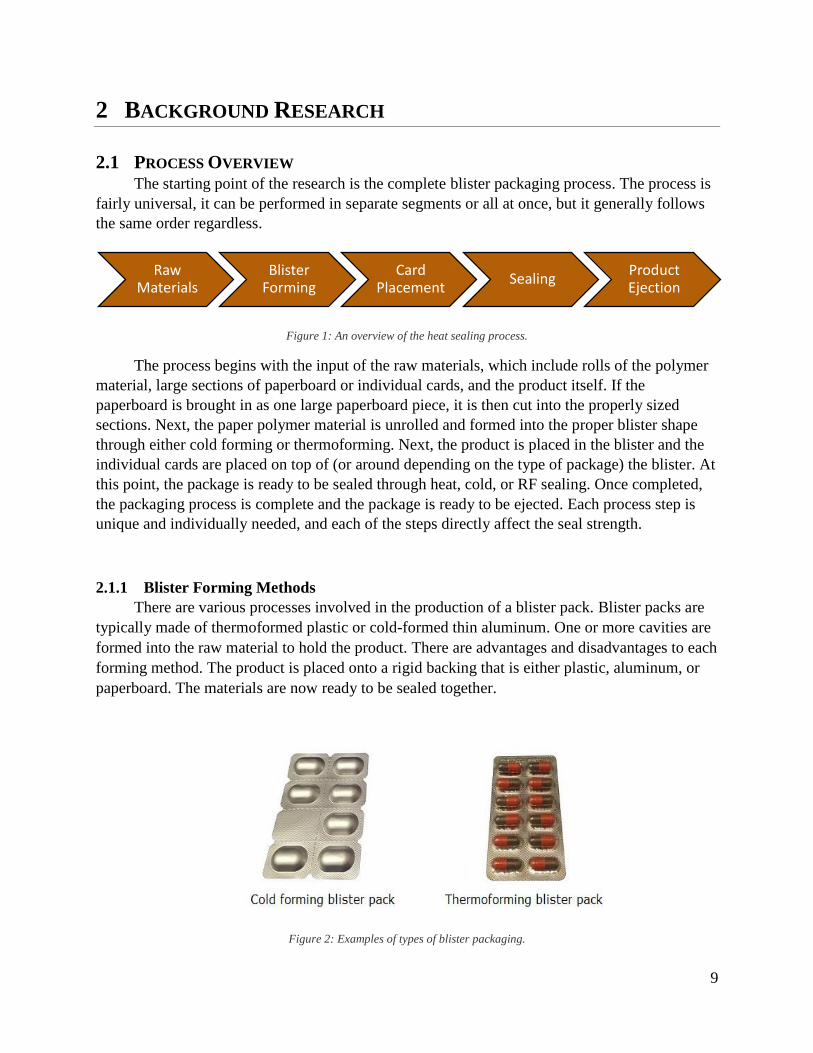
2.1 PROCESS OVERVIEW The starting point of the research is the complete blister packaging process. The process is
fairly universal, it can be performed in separate segments or all at once, but it generally follows
the same order regardless.
Figure 1: An overview of the heat sealing process.
The process begins with the input of the raw materials, which include rolls of the polymer
material, large sections of paperboard or individual cards, and the product itself. If the
paperboard is brought in as one large paperboard piece, it is then cut into the properly sized
sections. Next, the paper polymer material is unrolled and formed into the proper blister shape
through either cold forming or thermoforming. Next, the product is placed in the blister and the
individual cards are placed on top of (or around depending on the type of package) the blister. At
this point, the package is ready to be sealed through heat, cold, or RF sealing. Once completed,
the packaging process is complete and the package is ready to be ejected. Each process step is
unique and individually needed, and each of the steps directly affect the seal strength.
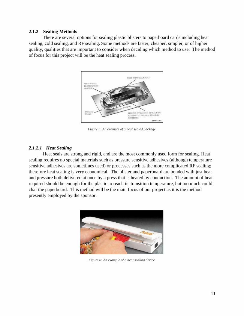
2.1.1 Blister Forming Methods
There are various processes involved in the production of a blister pack. Blister packs are
typically made of thermoformed plastic or cold-formed thin aluminum. One or more cavities are
formed into the raw material to hold the product. There are advantages and disadvantages to each
forming method. The product is placed onto a rigid backing that is either plastic, aluminum, or
paperboard. The materials are now ready to be sealed together.
Figure 2: Examples of types of blister packaging.

10
2.1.1.1 Cold Forming
Cold forming uses an aluminum film and can simply be stamped to shape without the use
of heat. The aluminum has better moisture and oxygen-barrier properties than plastic. Because
this process uses aluminum film instead of plastic, it is opaque. This process also requires a
larger paperboard card in order to properly seal because aluminum cannot be bent to 90 degree
angles without breaking. This process is also generally longer than thermoforming plastic
blisters. This method is more fit in pharmaceutical applications than in the packaging
applications of this project.
Figure 3: An example of blister packaging.
2.1.1.2 Thermoforming
Thermoforming begins with a roll of plastic heated to approximately its glass transition
temperature in order to soften it so that it can be easily formed. It is then placed over a mold and
air pressure forces the softened plastic to be pressed against the mold, often combined with a
plug-assist, or a negative of the mold used to help push the plastic uniformly into place with less
thinning of the plastic in the center. After a very short cooling period the plastic is ejected, now
capable of maintaining its new shape and is ready to be sealed to a paperboard card. The
benefits of this method are greater product visibility, greater strength as a result of using plastic
over aluminum foil, and the simplicity of its application compared to the use of foil. Benefits of
this method are greater product visibility, greater strength as a result of using plastic instead of
aluminum foil, and the simplicity of its application compared to the use of foil.
Figure 4: Examples of thermoformed packages.
11
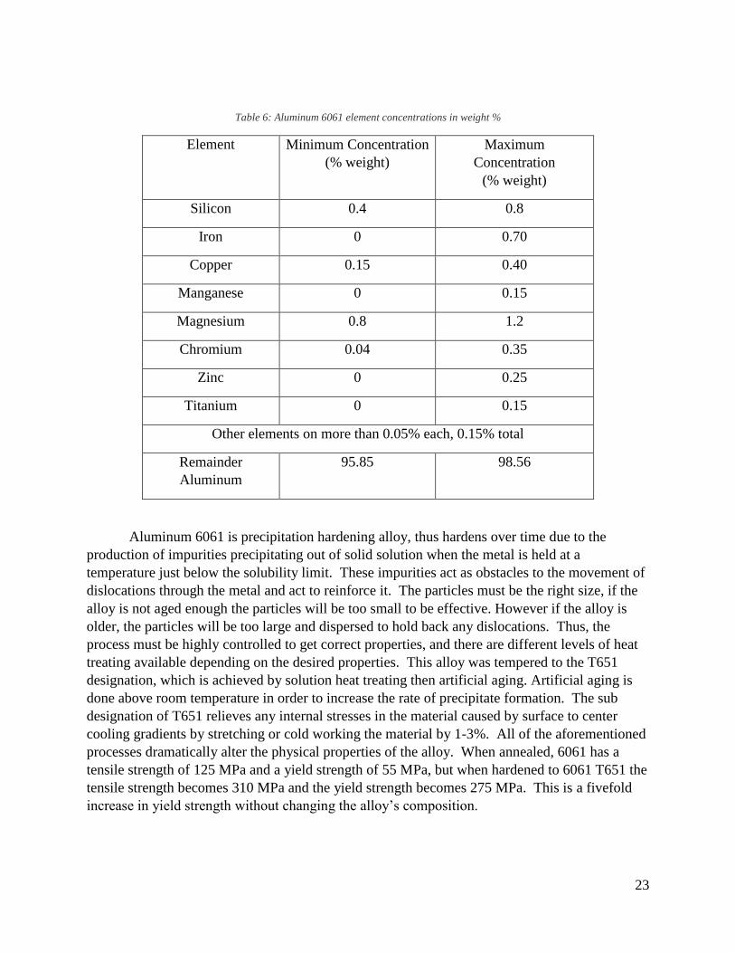
2.1.2 Sealing Methods
There are several options for sealing plastic blisters to paperboard cards including heat
sealing, cold sealing, and RF sealing. Some methods are faster, cheaper, simpler, or of higher
quality, qualities that are important to consider when deciding which method to use. The method
of focus for this project will be the heat sealing process.
Figure 5: An example of a heat sealed package.
2.1.2.1 Heat Sealing
Heat seals are strong and rigid, and are the most commonly used form for sealing. Heat
sealing requires no special materials such as pressure sensitive adhesives (although temperature
sensitive adhesives are sometimes used) or processes such as the more complicated RF sealing;
therefore heat sealing is very economical. The blister and paperboard are bonded with just heat
and pressure both delivered at once by a press that is heated by conduction. The amount of heat
required should be enough for the plastic to reach its transition temperature, but too much could
char the paperboard. This method will be the main focus of our project as it is the method
presently employed by the sponsor.
Figure 6: An example of a heat sealing device.

12
2.1.2.2 Cold Sealing
Unlike heat sealing, cold sealing needs only pressure to make a seal. A pressure-sensitive
coating, likely an adhesive, on the paperboard is necessary for a cold seal. The removal of the
temperature variable makes this a cold sealing a simpler process than heat sealing. Since there is
no heat, energy costs will be lower, and the process does not require a cool-down time. This
makes cold sealing a simple, fast, cost effective, and environmentally friendly sealing method,
but it also has the weakest bond strength of the three methods.
Figure 7: An example of a cold sealing process.
2.1.2.3 RF Sealing
RF sealing is much like heat sealing, except it uses high frequency radio waves to heat
the material. The radio waves (common frequencies range from 15 kHz to 70 kHz) cause the
molecules in the polymer to vibrate, producing a large amount of heat very quickly and evenly.
This leads to RF seals being faster, more uniform, and stronger than average heat seals. The
seals are also clear and unblemished making this method good for exposed seals. RF sealing
requires more precise equipment and more energy, making it more expensive than regular heat
sealing, however the RF field is rapidly developing and constantly becoming more efficient.
Figure 8: An example of RF sealing.

13
2.1.3 ASTM Standards
Experimental testing is essential in both the understanding of the effects and relationships
between the key parameters, and in the testing of the accuracy of an analytical model.
Seal strength is relevant to opening force and package integrity, but also the packaging
abilities to produce consistent seals. Current tests used by the sponsor for heat seals includes a
fiber tear test. The fiber tear test involves peeling off the seal of a paper cardboard, and measures
the surface area of the thermoblister with cardboard still attached. The amount of cardboard
fibers left behind give light to the strength of the seal but also the uniformity of its bonding. A
more quantifiable test to indicate this uniformity and strength of the seal is desired. Tensile
testing will show the force at which the seal breaks, which indicates the strength of that seal.
This more quantified and tangible test will be approximated by a combination of the
fundamentals of the tensile tests and a test similar to the previously mentioned “fiber tear test”.
Currently, no standard exist that meet these specific criteria.
While there are no ASTM standards that match this project’s application exactly, there
are two standards that come particularly close. The first ASTM standard available for this
application is “Standard Test Method for Seal Strength of Flexible Barrier Materials”,
Designation F88/F88M_09. This standard covers the measurement of seals in a flexible
materials; unfortunately, the standard F88/F88M_09 measures the strength of seals that are too
“flexible” for usage by the sponsor in this application.
During the process of the creation of a more relevant standard for this application,
fundamentals from testing procedures of other standards can be examined. Ideals should be taken
by the standards below to create a tests that are applicable for the sponsor:
For the current application the relevant concerns from ASTM F88:
Magnitude of Force: average force to open the seal should be the most useful, although
the maximum and minimum forces required may also be useful.
o If the test strip does not peel considerably in the seal area, average force to failure
may have little significance in describing seal performance and should not be
valued in such cases
Components of Force: The standard desired should include measurement of force when
testing materials may also be exposed to a bending component, and not just brute force
alone. Various fixtures should be organized and created in a way so to test these different
parameters for bending and force components needed to open a seal. The number of
samples should be chosen to ensure an accurate representation of performance of the seal.

14
Figure 9: Examples of ASTM Testing Procedures.[18]
Technique A: Unsupported: Each tail of sample is secured in opposite grips.
Technique B: Supported 90 (by hand): each tail of sample is secured in opposite grips and the
seal remains hand-supported at 90 perpendicular angle to the tails during testing.
Technique C: Supported 180: The least flexible tail is supported flat against a stiff alignment
plate held in one grip.
Testing of samples with deviations from normality should not be used in high numbers or
high regard as they may influence the process average in an unrealistic way. Essentially, a
combination of the peel testing, fundamental of the tensile and fiber tear testing, molded into a
capacity similar to the “Standard Test Method for Seal Strength of Flexible Barrier Materials”
should test the heal seal strength appropriately.
The second test specification relevant to this project is ASTM D903- 49, or “Standard
Test Method for Peel or Stripping Strength of Adhesive Bonds” and is a frequently used test to
measure the strength of adhesives. The test includes an adhesive pulled back at 180° from an
adherent. This standard is primarily useful for materials that require a small amount of stress to
fold them back (Shields).

15
Figure 10: ASTM standard for adhesive peel test.[18]
The test requires at least ten samples to be examined, to discard any outliers due to flaw,
and that the specimens be thick enough to tolerate tensile pulls, but their thickness should not
exceed 3mm. Figure 10 shows the test setup for the ASTM Standard D903-49 to determine the
strength of adhesives or bonding materials. A combination of the two aforementioned standards
will likely lead to the most relevant standard for this project.
Although not feasible for the scope of this project, a third means of testing for seal quality
and integrity lies the ASTM F3004-13e1 standard, or “Test Method for Evaluation of Seal
Quality and Integrity Using Airborne Ultrasound”.
The apparatus components include:
1. The components of the apparatus are a transducer (provides ultrasonic waves)
2. Air gap between signal and detection transducers
3. A transducer capable of detecting signal strength after passing through air gap
4. An instrument (hardware and software) capable of analyzing ultrasonic wave
information
5. Computer system to gather signal intensity information at any given location and
adapt it to usable form for the examiner
This test method can be applied to heat seals and the variety of package materials used in
packaging such as flexible, semi-rigid, and rigid components. This technology does not destroy
the package seal it is testing, is quantitative, and is objective. This testing method incorporates
technology that can be used to detect defects in seals based on the concept that poor quality seals
will not transit as much ultrasonic energy as correctly sealed packages.

16
This technique is also built on the principle that sound waves are transmittable at varying
speeds through different materials and as such, the denser materials experience faster wave
transmission. The standard explains the importance of acoustic impedance in that it is the
product of density and velocity and naturally can indicate a change in transmission material.
Users of this method should pay close attention to the drastic difference in impedance values for
a given material and air. This is a sure and easy way to detect the presence of air in the seal, and
can be indicative of a poor seal in that given area.
Table 1: Material vs. acoustic impedance value [19]
2.2 MATERIALS Once there was a solid understanding of the process as a whole, research was directed into
the depths of each section of the process to find their relevance to the strength of the seal. The
first part of the process to study was the materials used.
2.2.1 Paperboard
The first half of the material in blister packaging is the paperboard card that connects to
the polymer blister. There are many arrangements for blister and card, including simple card-to-
blister, clamshell, and folding or double card. Regardless of method, the polymer material is
bonded to the paperboard during the sealing process. The paperboard material itself is rarely of
consequence, due to the fact that most paperboard used in blister packaging is coated in some
laminate or adhesive. Paperboard materials consist mostly of bleached wood pulp that is layered
with polyethylene to increase its rigidity. Since the laminate or adhesive is what actually bonds
with the blister, it is much more important to understanding the sealing process. The paperboard
used by the Sponsor is the International Paper Everest High Visibility Packaging line Safepak 18
pt.
MaterialVelocity
(cm/ sec)
Density
(g/cm3)
Acoustic
Impedance
(g/cm2-μsec)
Air (20 C, 1 bar) 0.0344 0.00119 0.000041
Water (20°C) 0.148 1 0.148
Polyethelene 0.267 1.1 0.294
Aluminum 0.632 2.7 1.71

17
Table 2: Heat sealing relevant properties of SafePak 18pt
Table 3: Other properties of SafePak 18pt
2.2.2 Adhesives
An adhesive can be most broadly defined as any substance that sticks or glues materials
together. In this project, the adhesive layers in the assortment of raw materials is the most
contributing factor to the seal of the package. In regards to blister packaging, adhesives are used
to seal the paperboard to the plastic blister. There are several types of adhesives used in industry,
ranging from acrylic to cellulose derivative, from epoxy-based to rubber-based; oftentimes the
unique properties intrinsic to each adhesive type are further complicated when the adhesives are
blended before implementation. For the application seen in this project, Hot-melt adhesives are
most commonly seen.
The properties of this adhesive family make them an appropriate selection for the sealing
needs of the packaging. This group of materials are melted and upon cooling, they become solid
and have a greater resultant strength to adhere the two surfaces. They melt at lower temperatures
relative to other bonding agents, from 65 to 180 C. The Hot-melt adhesives are one of the most
widely accepted adhesives for the paper and packaging industry, in addition to the footwear and
plastic fields. Hot-melts are known for their ability to effectively adhere paper, board,
polypropylene, polyethylene, films, coatings, and other surfaces. They are economically a
reasonable option for many applications and their bonding efficacy depend largely on factors
such as presume, time, and temperature. They are able to be used in industry in a rapid and
effective manner, making them utilized at large manufacturing scales. Just as they vary in
application, naturally hot melts vary in shape and form. They available in tapes, films, blocks,
and can be used as solvent solutions to be heat-activated at a later time (Shields).
Heat Sealing Properties of Paperboard Heat Seal Temperature Range ( C) Heat Sealing Pressure Range (psi) Heat Sealing Dwell Time (Seconds)
SafePak 18pt 250 to 400 40 to 120 1 to 2.5
Various Paperboard Properties Bais Weight Moisture % Stiffness, Taber V-5 Gloss (75 ) (Coated Side)
SafePak 18pt 264 (lbs./3000 (Sq.ft)) 279 (MD gcm)
430 (GMS) 155 (CD gcm)
22.0 (0.001 inch) 27.4 (MD mNm)
0.559 (Mm) 15.2 (CD mNm)
Brightness % ( Coated Side) Coefficient of Friction Smoothness PPS (10) (Coated Side) Tear Emendorf, gms
0.59 (Kinetic) 1,018 (MD)
0.57 (Static) 1,149 (CD)
5.558
87 1.2

18
2.2.3 Polymers
The second half of the package, the blister, is composed of a polymer. The word polymer
literally means many monomers. Monomers are essentially molecule links of a certain
composition that are bonded together to form long repeating chains, the polymers.
Polymers are a fairly recent material category compared to metals and ceramics. After
their introduction, they became one of the most used materials in the entire world, mainly due to
their unique and diverse properties. Advantages of plastics include low cost, resistance to
corrosion and chemicals, low thermal and electrical conductivity, low density, and high strength
to weight ratios. Polymers are made in a chemical process called a polymerization reaction, of
which there are two main methods. The first is condensation polymerization, where the polymer
if formed by mixing two reacting monomer molecules. The reaction between the molecules
bonds them together while producing some form of byproduct, such as water. The other method
is known as addition polymerization. In this method, there is either only one type of monomer
molecule or two unreactive molecules. An initiator is introduced which reacts with the
molecule(s) and bonds with them. Once bonded, a chain reaction starts where the bonded
monomer opens up another available connection, which can then connect with another monomer
or initiator.
Figure 12: An example of molecular chains.
The ratio of initiator to monomer molecules determines the length of the chain, as an
open monomer will more likely bond with another monomer if there is a large number of them.
The size of these polymer chains can be expressed by the degree of polymerization, which is a
ratio of the molecular weight of the polymer to the weight of the individual monomer.
Figure 11: The Mer structures of PP, PE and PS.

19
2.2.4 Thermosets vs Thermoplastics
There is a very important distinction to make in the world of polymers, the difference
between thermosets and thermoplastics. Before obtaining a specific list of polymers used in this
project, it was important to understand which of these designations the specified polymers would
fall under. Thermosets are defined as polymeric materials that “cure” during heating and become
fixed after cooling. When the polymer is heated, the molecule chains that form the polymer
become cross-linked. This means that the polymer cannot be reheated and melted back down into
its previous form. This makes thermosets highly unrecyclable and overall a hindrance in the
blister packaging process. The main reason for this hindrance is the fact that the polymer can be
heated twice throughout the process. Using a thermoset polymer would limit the combinations of
blister forming and sealing methods that could be used. Additionally, the fact that thermosets
cannot be “reset” easily means they cannot be recycled. Companies that wish to improve the
environmental effects of their productions will have a hard time utilizing the unrecyclable
thermosets. Thermoplastics on the other hand are entirely free to be reheated and reformed. They
do not form the irreversible cross-links, and are therefore free to be recycled a large number of
times, making them much more attractive option for the blister packaging process than
thermosets. Not only do thermoplastics allow for any combination of blister forming and sealing
methods to be used, but they provide the option for a large amount of recyclability for
companies. However, thermoplastic materials are generally weaker as a result of the lack of
cross-linked polymer chains. They have worse mechanical properties, resistances to chemicals,
and overall lower durability than their thermoset counterparts.
2.2.5 Common Materials
Now that that there was an understanding that the polymers used in the blister packaging
process would fall under the thermoplastic category, the research was direction into specific
materials that are used. The first material found was polyvinyl chloride (PVC). PVC was a very
popular material used in product packaging, mainly because of it was easy to thermoform and
was relatively cheap to produce. However, PVC packaging resulted in very weak barrier
properties, namely water and oxygen resistance. This limited PVC’s usage in industries such as
pharmaceuticals where these properties were important.
Figure 13: Mer structure representation of PVC.

20
Additionally PVC has a wide range of environmentally and medically harmful effects due
mainly to the chlorine atom that composed part of its monomer. These effects ranged from
release of micro-particles into the air during degradation to carcinogenic classification of the
vinyl chloride monomer that constitutes PVC. For these reasons PVC on its own saw less usage.
However, other polymer materials could be added to PVC in layers to enhance some of its
properties. One such polymer is polychlorotrifluoroethylene (PCTFE). PCTFE’s main advantage
is that it corrects the weak barrier properties that PVC exhibited. This lead to PCTFE seeing
widespread use in the pharmaceutical industry. However, even with layering, PCTFE still
displayed many unfavorable characteristics. The developments in cyclic olefin copolymers
(COC) lead to advances in packaging materials that began to steer away from PVC. COCs
provided a material that had many advantages over PVC, including excellent barrier properties
and vastly reduced harmful effects on both the environment and humans. Additionally COCs
have impressive levels of transparency and a higher allowance on aspect ratio. This makes COCs
very glasslike, and suitable for the optical industry. Furthermore, COCs could be combined with
various other polymers used in packaging, such as polyethylene (PE), polypropylene (PP), and
polyethylene terephthalate (PET) to improve their barrier characteristics while maintaining their
individual strengths.
2.2.6 Amorphous Polyethylene Terephthalate (aPET)
During the research on materials the Sponsor was contacted for information on specific
materials that they used in their blister packaging. Like much of the industry, they too were
moving away from using PVC in their packaging due to its harmful effects. The Sponsor focuses
on aPET or amorphous polyethylene terephthalate for their packaging polymer. aPET consists of
chains of the ethylene terephthalate monomers (C10H8O4) and is used in a variety of plastic
products, including blister packaging.
Figure 14: Mer structure representation of aPET.
PET is the third most commonly produced polymer behind polyethylene and
polypropylene, and when produced as a fiber it is commonly referred to as polyester. PET is
polymerized through a water producing condensation reaction that first transitions through either
an esterification or a transesterification reaction in order to form its monomer bis(2-

21
hydroxyethyl) terephthalate (C12H14O6). The esterification reaction is produced from
terephthalic acid (C8H6O4) and ethylene glycol (C2H6O2) with water as a byproduct, Figure 15,
Figure 15: Esterification reaction with water byproduct.
and the transesterification reaction is produced from dimethyl terephthalate (C6H4(CO2CH3)2) and
ethylene glycol (C2H6O2) with methanol as a byproduct, Figure 16.
Figure 16: Transesterification reaction with methanol byproduct.
The amorphous in the name signifies a material with a low crystallinity. Crystallinity is
the level of grid formation in a polymer’s structure. The higher the crystallinity the more rigid a
material becomes, while also increasing its opaqueness. Since a large part of product packaging
is being able to display the product on store shelves, it is important to utilize this low crystallinity
for blisters. Additionally, aPET is lightweight and impact resistant, with a high level of
recyclability. This makes it an excellent material for blister packaging.

22
Table 4: Properties of Pentaform® SmartCycle® Ridge APET TH-Es135R
Table 5: Properties for Roll Stock – ecostarTM Bio-HS 1000 (multilayer)
2.2.7 Aluminum
The particular type of aluminum used in the experiments was 6061-T651. This was
chosen for its thermal and physical properties in order to closely match those of the undisclosed
aluminum alloy used in the Sponsor’s press. These properties include high machinability,
relatively high strength, ease of acquisition, and most importantly, high thermal conductivity.
Due to these material properties, a sturdy press capable of transferring large amounts of heat was
easily machined. Aluminum 6061 is a mixture of various concentrations of elements as seen in
Table 6.
Unit Value Unit Value
Gauge Range Available Micrometer Mil 10-40 Micron 254-1,016
Gauge Tolerance D-374 % ±5 % ±5
Specific Gravity D-792 - 1.33 - 1.33
Tensile Stength D-882 in2/lb 7200 N/mm2 50
Tensile Modulus of Elasticity D-882 in2/lb 300,000 N/mm2 2,068
Heat Deflection Temperature D-648 F 149 C 65
2.96
1.98
1.48
Properties StandardU.S. SI
Material Yield (Nominal)
10 mil
15 mil
20 mil
D-792 in2/lb
2,080
1,390
1,040
m2/kg
Property Units
ECOSTAR TM HS1000
COEXTRUDED Target
Values
Test
System
Test
Method
Clarity (Percentage) > 95 ASTM D 1003
Tensilt Strength @ Break psi > 7000 ASTM D 638
Izod Impact Strength ft-lbs/in 1 to 2 ASTM D 256
Heat Deflection Temperature F 150 ASTM D 648
Dart Impact @ 73 F (20 MIL) grams > 500 ASTM D 1709
Specific Gravity N/A 1.33 ASTM D 792
Color. B Value N/A 0 to 2.0 ASTM D 1003
Gauge mil See Master Specification N/A N/A
Haze (20 MIL) (Percentage) < 4.0 ASTM D 1003
Intrinsic Viscosity dl/g > 0.74 ASTM D 1236
Flexural Modulus psi > 300,000 ASTM D 790
23
Table 6: Aluminum 6061 element concentrations in weight %
Element Minimum Concentration
(% weight)
Maximum
Concentration
(% weight)
Silicon 0.4 0.8
Iron 0 0.70
Copper 0.15 0.40
Manganese 0 0.15
Magnesium 0.8 1.2
Chromium 0.04 0.35
Zinc 0 0.25
Titanium 0 0.15
Other elements on more than 0.05% each, 0.15% total
Remainder
Aluminum
95.85 98.56
Aluminum 6061 is precipitation hardening alloy, thus hardens over time due to the
production of impurities precipitating out of solid solution when the metal is held at a
temperature just below the solubility limit. These impurities act as obstacles to the movement of
dislocations through the metal and act to reinforce it. The particles must be the right size, if the
alloy is not aged enough the particles will be too small to be effective. However if the alloy is
older, the particles will be too large and dispersed to hold back any dislocations. Thus, the
process must be highly controlled to get correct properties, and there are different levels of heat
treating available depending on the desired properties. This alloy was tempered to the T651
designation, which is achieved by solution heat treating then artificial aging. Artificial aging is
done above room temperature in order to increase the rate of precipitate formation. The sub
designation of T651 relieves any internal stresses in the material caused by surface to center
cooling gradients by stretching or cold working the material by 1-3%. All of the aforementioned
processes dramatically alter the physical properties of the alloy. When annealed, 6061 has a
tensile strength of 125 MPa and a yield strength of 55 MPa, but when hardened to 6061 T651 the
tensile strength becomes 310 MPa and the yield strength becomes 275 MPa. This is a fivefold
increase in yield strength without changing the alloy’s composition.

24
(a) (b)
Figure 17: (a) Aluminum 6061, 550 x 50 pancake grain structure, (b) The microstructural phases of Aluminum 6061.
2.3 HEAT TRANSFER IN RELATION TO HEAT SEALING
2.3.1 Conductive Heat Transfer
The transfer of thermal energy which occurs between the heat sealing plate and the
multiple layers of packaging material is essential towards understanding how the seal process
happens and the strength of the seal itself. The study of heat transfer and the application of
various fundamental equations will allow for a model to be built which can relate the process
parameters of material thickness, temperature and time to the material properties of the
packaging materials.
The primary equation which can properly represent the rate of heat transfer through a
multi-layered body is Fourier’s Law of heat conduction. The following image and equations
show an example of Fourier’s law as it is applied to a multi-layer situation.
Tn Temperature at a given boundary n
kn Thermal conductivity of layer n
bn Thickness of layer n
Q The heat being transferred through the system
A Surface area of the work piece
𝑇1 − 𝑇2 =𝑏1
𝑘1𝐴𝑄 𝑇2 − 𝑇3 =
𝑏2
𝑘2𝐴𝑄 𝑇3 − 𝑇4 =
𝑏3
𝑘3𝐴𝑄
𝑇1 − 𝑇4 = (𝑏1
𝑘1𝐴+
𝑏2
𝑘2𝐴+
𝑏3
𝑘3𝐴)𝑄
Figure 18: An explanation of Fourier’s law.

25
Fourier’s law provides a mathematical correlation between the thermal conductivities of
the various materials used in the sealing process and the activation energy which is needed to
insure that the effects of the adhesive are activated. Using derivations of this equation in tandem
with the computational methods mentioned later in the report, fundamentals based models for the
heat sealing process and seal strength which are driven by the key process and material
parameters will be constructed.
For the purposes of this project, the following is a representation of the number and types
of boundaries which will be of concern for the heat transfer.
The current assumption is that the heat will be applied from above via a heated press plate
which is heated up before making contact with the desired sealing surface. The press plate must
reach a temperature which will result in the proper amount of heat transferring through the layers
in order to insure that both adhesive layers reach their activation energies. Another simple way of
looking at the situation is to use a circuit equivalent system, where each layer provides resistance
to the heat transfer through the package. This resistance would have the following setup:
𝑄 =∆𝑇
∑ 𝑅=
∆𝑇
𝑅𝑃𝑎𝑝𝑒𝑟 + 𝑅𝐴𝑑ℎ𝑒𝑠𝑖𝑣𝑒 + 𝑅𝑃𝑙𝑎𝑠𝑡𝑖𝑐
Figure 19: Heat transfer relevant to the sealing process.

26
2.3.1.1 Contact Resistance
Figure 20: Physical representation of contact resistance.[8]
The resistance equivalent sheds light on one area of difficulty when considering the
conduction of heat through multiple surfaces in direct contact with one another. This difficulty is
the way in which heat is transferred across the contact points between the materials. At first
thought, it may seem that using the summation of resistance values of the materials being
considered would be adequate for the calculation of the heat transfer. However, due to differing
surface metrologies, it is highly unlikely that two materials are in full contact. Instead, pockets of
vacuum or fluid can form in-between two materials, thus resulting in an increase in the thermal
resistivity of the overall system. These cavities result in the need to consider new resistance
terms besides those of the materials themselves, where there may not only be conduction
occurring, but convection and/or radiation as well. The concept of contact resistance is one
which is not currently well understood, and requires much unique experimentation and data
collection to calculate values for individual specific material interactions (Williamson).
2.3.2 Transient Heat Transfer
Transient Heat conduction applications are heat transfer applications that acknowledge
that temperature changes from changes in position and passing time. Transient heat transfer
equations therefore evaluate systems where temperature is not evenly distributed throughout the
system, such as temperature differences through layers of paperboard and adhesive. The transient
heat transfer equations includes the Fourier number which describes the heat conduction, but also
the Biot (Bi) number, which describes the transient (time specific) aspect of an application. The
application of the transient heat transfer equation is to gain better insight on specific
temperatures of specific layers within the paperboard and adhesive system at a specific point in
time.

27
Table 7: Variables from Bi and Fo Equations
𝑭𝒐 Fourier Number
α Thermal diffusivity (
m2
s)
t Time (s)
L Unit of length (m)
𝑳𝒄 Characteristic length (m)
V Volume (m3)
h Film coefficient, or heat transfer coefficient (W
m2∗K)
A Surface area (m2)
𝑻𝟎 Initial temperature, T at t=0 (K or °C)
𝑻∞ Temperature at infinity or ambient temperature (K or °C)
T Temperature at specific point in time that is not 0 seconds (K or °C)
𝒌𝒃 Thermal conductivity of body (W
m∗K)
𝒄𝒑 Specific heat capacity (J
K )
ρ Density (kg
m3)
The Biot number is a dimensionless number that relates the heat transfer coefficient,
characteristic length, and thermal conductivity of the material being examined.
𝐵𝑖 =ℎ𝐿𝑐
𝑘𝑏
Where the characteristic length, or Lc, is defined as
𝐿𝑐 =𝑉𝑏𝑜𝑑𝑦
𝐴𝑠𝑢𝑟𝑓𝑎𝑐𝑒
If the Biot number is less than 0.1 in many applications, the system can be assumed to be
lumped. A lumped system assume uniform temperature distribution, and the smaller the Biot
number, the more accurate this assumption is. For applications where the Biot number is above
0.1, a uniform temperature distribution cannot be assumed, and temperature changes with
changes in time and position.
The Fourier number (Fo) is also a dimensionless number that relates thermal diffusivity,
characteristic time, and length of material through which conduction occurs.
𝐹𝑜ℎ =𝛼𝑡
𝐿2
where
28
𝛼 =𝑘
𝜌𝑐𝑝
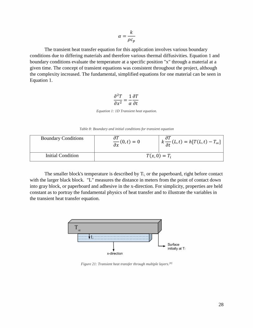
The transient heat transfer equation for this application involves various boundary
conditions due to differing materials and therefore various thermal diffusivities. Equation 1 and
boundary conditions evaluate the temperature at a specific position "x" through a material at a
given time. The concept of transient equations was consistent throughout the project, although
the complexity increased. The fundamental, simplified equations for one material can be seen in
Equation 1.
𝜕2𝑇
𝜕𝑥2=
1
𝛼
𝜕𝑇
𝜕𝑡
Equation 1: 1D Transient heat equation.
Table 8: Boundary and initial conditions for transient equation
Boundary Conditions 𝜕𝑇
𝜕𝑥(0, 𝑡) = 0 𝑘
𝜕𝑇
𝜕𝑡(𝐿, 𝑡) = ℎ[𝑇(𝐿, 𝑡) − 𝑇∞]
Initial Condition 𝑇(𝑥, 0) = 𝑇𝑖
The smaller block's temperature is described by Ti, or the paperboard, right before contact
with the larger black block. "L" measures the distance in meters from the point of contact down
into gray block, or paperboard and adhesive in the x-direction. For simplicity, properties are held
constant as to portray the fundamental physics of heat transfer and to illustrate the variables in
the transient heat transfer equation.
Figure 21: Transient heat transfer through multiple layers.[8]

29
2.3.3 Free Convection
Free or natural convection is the cooling of a body due to buoyancy forces of the air. The
buoyancy forces are due to differences in densities between hot and cooler air. As the fluid
surrounding a hot object heats up, it begins to rise, leaving the cooler fluid to sink beneath it, and
the cycle continues. Natural convection depends on the Rayleigh number, or Ra, as forced
convection depends on the dimensionless Reynolds number (Re).
Due to the complexity of finding an accurate convection coefficient value, there is very
little literature available to account for the press movement from its initial position to the surface
of the raw materials. Literature suggests that convection coefficients of natural convection in
gases range between 1 [W/(m2K)] and 20 [W/(m2K)]. To acquire a closer estimate of an
appropriate “h” value, two experts in the field were consulted for their input on the calculations.
These consulting WPI faculty are Professor Germano Iannacchione and Professor John Sullivan.
Professor Germano Iannacchione shed insight on the complex problem by suggesting the
press movement be modeled as free convection. The press has a 0.12 m/s velocity, and due to the
ridged and indented characteristics of the press trapping the near 400°F air, the heat loss is going
to be minimal. He suggested that’s the “h” value be considered as any value from 5 to 10
[W/(m2 K)].
Professor John Sullivan had a similar view of the assumption. With these very low
speeds, the air flow around the press is going to be in the laminar range. Sullivan suggested that
research be conducted towards how little the difference in heat transfer varies from an “h” value
of 0 to 10. Because of this very small difference in heat loss with convection coefficients
between 0 and 10 [W/(m2 K)] the average of these coefficient values, 5 was used. With this,
Sullivan also suggested that this movement and set of conditions should be modeled as free
convection.
2.3.4 Heat Diffusion Equation
Based on conditions imposed on a system’s boundaries, a temperature distribution can be
determined from conduction analysis. Once the temperature distribution is determined, heat flux
can be computed at any point or surface via the Fourier’s law. The best approach towards solving
an accurate temperature distribution includes considering a differential control volume, relevant
energy transfer processes, and appropriate rate conditions.
Examine a homogeneous medium where there is no convection or radiation, and the
temperature is expressed in Cartesian coordinates T(x,y,z). The conservation of energy theory is
applied, a differential control volume 𝑑𝑥 ∗ 𝑑𝑦 ∗ 𝑑𝑧 is examined. Energy processes considered at
an instance in time are considered with respect to the conservation of energy. The problem
operates under the assumption that there is no energy or work being done on the system, and
only thermal energy is transferred externally. Conduction heat rates that are perpendicular to
each of the volume's surfaces are indicated by qx, qy, and qz on the x-,y-,z-planes respectively.

30
Table 9: Heat transfer equation variables
Variable Units
𝒒 Heat [𝐽
𝑘𝑔∗𝐾]
𝝆 Density [𝑘𝑔
𝑚3]
𝒄𝒑 Specific heat Capacity [𝐽
𝑘𝑔∗𝐾]
𝒌 Thermal conductivity, [𝑊
𝑚∗𝐾]
𝑻 Temperature [K]
�� Energy Source [K*J]
𝜶 Thermal diffusivity [𝑚²
𝑠]
𝒕 Time [s]
The Taylor series expansion can be used to express the heat conduction rates at the
opposite surfaces as seen in Equation 2, Equation 3, and Equation 4.
𝑞𝑥+𝑑𝑥 = 𝑞𝑥 +𝜕𝑞𝑥
𝜕𝑥𝑑𝑥
Equation 2: Heat conduction rate in x dimension.
𝑞𝑦+𝑑𝑦 = 𝑞𝑦 +𝜕𝑞𝑦
𝜕𝑦𝑑𝑦
Equation 3: Heat conduction rate in y dimension.
𝑞𝑧+𝑑𝑧 = 𝑞𝑧 +𝜕𝑞𝑧
𝜕𝑧𝑑𝑧
Equation 4: Heat conduction rate in z dimension.
For this project’s application, the energy source term �� associated with the rate of energy
generation is zero.
Using the conservation of energy, the conduction equation can be seen in Equation 5:
𝑞𝑥 + 𝑞𝑦 + 𝑞𝑧 + ��𝑑𝑥𝑑𝑦𝑑𝑧 − 𝑞𝑥+𝑑𝑥 − 𝑞𝑦+𝑑𝑦 − 𝑞𝑧+𝑑𝑧 = 𝜌𝑐𝑝
𝜕𝑇
𝜕𝑡𝑑𝑥𝑑𝑦𝑑𝑧
Equation 5: Conduction equation with conservation of energy.

31
The following equation can be evaluated by substituting equations in Equations 2, 3, and 4.
−𝜕𝑞𝑥
𝜕𝑥𝑑𝑥 −
𝜕𝑞𝑦
𝜕𝑦𝑑𝑦 −
𝜕𝑞𝑧
𝜕𝑧𝑑𝑧
Where
𝑞𝑥 = −𝑘𝑑𝑦𝑑𝑧𝜕𝑇
𝜕𝑥
𝑞𝑦 = −𝑘𝑑𝑥𝑑𝑧𝜕𝑇
𝜕𝑦
𝑞𝑧 = −𝑘𝑑𝑥𝑑𝑦𝜕𝑇
𝜕𝑧
By substituting the previous three equations into Equation 5, Equation 6 is obtained, the
heat transfer diffusion equation in its general form, in Cartesian coordinates:
𝜕
𝜕𝑥(𝑘
𝜕𝑇
𝜕𝑥) +
𝜕
𝜕𝑦(𝑘
𝜕𝑇
𝜕𝑦) +
𝜕
𝜕𝑧(𝑘
𝜕𝑇
𝜕𝑧) + �� = 𝜌𝑐𝑝
𝜕𝑇
𝜕𝑡
Equation 6: General heat diffusion equation.
From the solution of the heat transfer equation, temperature distributions (x, y, and z) are
explored as a function of time. The heat transfer equation emphasizes the conservation of energy,
and “at any point in the medium the net rate of energy transfer by conduction into a unit volume
plus the volumetric rate of thermal energy generation must equal the rate of change of thermal
energy stored within the volume” (Bergman, 2011, 80).
As mentioned previously, Equation 6 refers to the heat transfer equation in its most
general form. If the thermal conductivity is constant, the heat equation can be simplified to
Equation 7(a)
𝜕2𝑇
𝜕𝑥2+
𝜕2𝑇
𝜕𝑦2+
𝜕2𝑇
𝜕𝑧2+
��
𝑘=
1
𝛼
𝜕𝑇
𝜕𝑡
Equation 7(a): Heat diffusion equation with constant thermal diffusivity.

32
where 𝛼 =𝑘
𝜌𝑐𝑝 is the thermal diffusivity. A consistent thermal diffusivity would be
applicable in cases where the density, specific heat, and thermal conductivity is constant in each
of the three Cartesian directions, most commonly when only one fluid or material is used.
Steady state conditions can also simplify the heat transfer equation. Steady state
conditions are when there is no change in the amount of energy storage in system. When steady
state conditions are applied to the heat transfer equation, the equation is reduced to
𝜕
𝜕𝑥(𝑘
𝜕𝑇
𝜕𝑥) +
𝜕
𝜕𝑦(𝑘
𝜕𝑇
𝜕𝑦) +
𝜕
𝜕𝑧(𝑘
𝜕𝑇
𝜕𝑧) + �� = 0
The simplest and most fundamental form of this heat transfer equation is a one-
dimensional problem that is under steady state conditions. In that case, the equation drastically
reduces to
𝜕
𝜕𝑥(𝑘
𝜕𝑇
𝜕𝑥)
in the x-direction, for example. It is important to note that in a steady state, one dimensional
problem with no energy generation, the heat flux is a constant in the direction of the heat
transfer.
For heat transfer through a medium in two directions (x and y, for example) in steady state
conditions through a single medium as seen in Equation 8:
𝜕2𝑇
𝜕𝑥2+
𝜕2𝑇
𝜕𝑦2=
1
𝛼
𝜕𝑇
𝜕𝑡
Equation 8: 2D heat diffusion equation with no internal heat generation.
Being able to understand and apply the fundamentals of heat transfer is essential to
analyzing the problem at hand, and this equations provides a solid foundation to solving the
problem.

33
3 ANALYTICAL INTERPRETATIONS
3.1 INITIAL HEAT TRANSFER CONFIGURATION The setup for this project reflected a transient conductive heat flow through multiple
layers of material. The first step for solving a problem is to setup the condition experienced, and
Figure 22 gives a simple one dimensional view of a conduction equivalency to the problem
described.
The three different layers in the figure represent the three layers found in the typical blister
packages featured in this project. As can be seen in Figure 22, the heat is first transferred to a
layer of paperboard, then adhesive, plastic, a second layer of adhesive, and then a final layer of
paperboard. Next, a set of boundary conditions will need to be developed to describe what
happens at the edge of this setup.
The first of these boundaries layers concern the bottom and side layers of the package,
where each were equated to insulation. This means that these interfaces will provide no heat
transfer between the boundary and the layers of the packaging. This condition was chosen to help
simplify the problem to a solvable state, but also due to the fact that the heat loss through these
layers should be relatively low compared to the flow of heat into the package from the press.
The final boundary layer condition to be determined is the upper interface where heat is
being applied to the system. To further the simplification of the setup, an assumption was made
that there was perfect heat transfer through the contact between the press and the first paperboard
layer. Furthermore, it was determined that this heat transfer could be described as a constant
temperature or temperature gradient at the top boundary representing the press. The assumption
that this temperature or temperature gradient would not change much with time as the process
went on was based on the idea that the thermal mass of the press system would be much larger
than the system of the package receiving this heat. This means that the press system will have
large reserves of heat in its own mass that can be used to replenish the surface temperature and
keep it from falling. To show what temperature changes would occur, the following thermal
mass comparison was used.
(𝑚𝑐𝑝∆𝑇)𝑝𝑎𝑐𝑘𝑎𝑔𝑒 𝑠𝑦𝑠𝑡𝑒𝑚 = (𝑚𝑐𝑝∆𝑇)𝑝𝑟𝑒𝑠𝑠 𝑠𝑦𝑠𝑡𝑒𝑚
Heat
Paperboard
Plastic Adhesive
Figure 22: 1D representation of conduction through multiple layers.

34
This equation represents the fact that any temperature change in the package will have a
relative change in temperature of the press system itself. The easiest way to visualize this change
is by looking at the mass and specific heat of each system. First, the mass of the press system
will be much larger than the mass of the package system. The package consists of five very small
layers of low mass components, while the press is a large and solid piece of aluminum connected
to a larger series of blocks that represent the heating component and the mechanisms to move the
press. Next, the specific heat for both system are of the same magnitude.
Given the following values of specific heat:
𝑐𝑝 𝑝𝑙𝑎𝑠𝑡𝑖𝑐 = 0.875𝐾𝐽
𝑘𝑔 𝐾
𝑐𝑝 𝑎𝑑ℎ𝑒𝑠𝑖𝑣𝑒 = 1.645𝐾𝐽
𝑘𝑔 𝐾
𝑐𝑝 𝑝𝑎𝑝𝑒𝑟𝑏𝑜𝑎𝑟𝑑 = 1.4𝐾𝐽
𝑘𝑔 𝐾
𝒄𝒑 𝒑𝒂𝒄𝒌𝒂𝒈𝒆 𝒂𝒗𝒆𝒓𝒂𝒈𝒆 =0.875 + 1.654 + 1.4
3= 𝟏. 𝟑𝟎𝟗
𝑲𝑱
𝒌𝒈 𝑲
𝒄𝒑 𝒂𝒍𝒖𝒎𝒊𝒏𝒖𝒎 = 𝟎. 𝟗𝑲𝑱
𝒌𝒈 𝑲
The combination of the specific heat values being close to one another and the mass of
the press system being much greater than the mass of the package system means the change in
temperature of the press will be relatively low to the change in temperature of the package.
Therefore, the assumption that the press’s surface remains at a constant temperature or
temperature gradient throughout the process is adequate.
This satisfies all of the boundary conditions for the package system. The result is a
transient conduction problem through layers with a constant surface temperature on one side and
all other sides being insulated. Figure 23 shows a visualization of the problem.
Constant Temperature
Insulated Heat Transfer Figure 23: Heat transfer of package system.

35
3.2 NUMERICAL SOLUTION For transient conduction problems there is one defining equation that can be applied to
systems with constant properties and no internal heat generation. This three dimensional version
of the equation is shown in Equation 7(b) and its origin is detailed in the background research
section 2.4.4.
1
𝛼
𝜕𝑇
𝜕𝑡=
𝜕2𝑇
𝜕𝑥2+
𝜕2𝑇
𝜕𝑦2+
𝜕2𝑇
𝜕𝑧2
Equation 7(b): Three dimensional heat diffusion equation with no generation.
While this equation is a good starting point, it cannot be used to analytically solve the
problem concerned in this project. Those produced solutions are only valid for cases with simple
boundary conditions, and is often only useful for one dimensional cases. While some cases of
two dimensional and three dimensional cases are possible, the problem presented in this project
is too complex for an analytical solution. The main deviation comes from the thermal diffusivity,
which is required to be constant if the equation is to be solved analytically. Since the package
system is comprised of layers of three different materials it will not have a constant thermal
diffusivity across the board. Therefore, instead of finding an analytical solution to this problem a
finite difference method was used.
To begin, both the physical and temporal aspects of the problem must be discretized,
therefore the subscripts m and n are selected to represent the position of discrete nodal points,
while p represents the discretization in time, where:
𝑡 = 𝑝∆𝑡
Beginning with Equation 7(b):
1
𝛼
𝜕𝑇
𝜕𝑡=
𝜕2𝑇
𝜕𝑥2+
𝜕2𝑇
𝜕𝑦2
where the finite-difference approximation can be expressed as the following three equations, two
for each dimension in space, and one in time.
𝜕2𝑇
𝜕𝑥2 |
𝑚,𝑛
≈
𝜕𝑇𝜕𝑥
|𝑚+
12
,𝑛−
𝜕𝑇𝜕𝑥
|𝑚−
12
,𝑛
∆𝑥
Equation 9: Finite difference approximation of the x dimension.

36
𝜕2𝑇
𝜕𝑦2 |
𝑚,𝑛
≈
𝜕𝑇𝜕𝑦
|𝑚,𝑛+
12
−𝜕𝑇𝜕𝑦
|𝑚,𝑛−
12
∆𝑦
Equation 10: Finite difference approximation of the y dimension.
𝜕𝑇
𝜕𝑡 |
𝑚,𝑛≈
𝑇𝑚,𝑛𝑝+1 − 𝑇𝑚,𝑛
𝑝
∆𝑡
Equation 11: Finite difference approximation of the time dimension.
As stated previously, the superscript p represents an instance in time while p+1 denotes
the next instance of time. This is due to the dependence on time that temperature of a nodal point
will have during a transient situation. Furthermore, this means that the numeric solution can only
be used to solve for temperatures are specific time and spatial locations moving forward with
time, as this is a forward-difference approximation. This is represents an explicit method
solution, as the current temperature is solved for using the previous temperature. This is highly
desired in the context of this project, as the starting temperatures of all parts of the system are
known. Equation 9 can be further solved by expressing the temperature gradients with the
following:
𝜕𝑇
𝜕𝑥 |
𝑚,+12
𝑛≈
𝑇𝑚+1,𝑛 − 𝑇𝑚,𝑛
∆𝑥
𝜕𝑇
𝜕𝑥 |
𝑚,−12
𝑛≈
𝑇𝑚,𝑛 − 𝑇𝑚−1,𝑛
∆𝑥
Taking these expressions and replacing the gradients in Equation 9, results in the following:
𝜕2𝑇
𝜕𝑥2 |
𝑚,𝑛
≈𝑇𝑚+1,𝑛 + 𝑇𝑚−1,𝑛 − 2𝑇𝑚,𝑛
(∆𝑥)2
Equation 12: Finite difference representation of x dimensional partial derivative.
Performing the same procedure for the y dimension produces a similar equation:

37
𝜕2𝑇
𝜕𝑦2 |
𝑚,𝑛
≈𝑇𝑚,𝑛+1 + 𝑇𝑚,𝑛−1 − 2𝑇𝑚,𝑛
(∆𝑦)2
Equation 13: Finite difference representation of x dimensional partial derivative.
Recalling Equation 8, the right hand side can be replaced with Equations 12 and 13 where the
superscript p can be added to represent that they are all concerned with the same instance of
time. Meanwhile the left hand side is replaced with its own equivalent.
1
𝛼
𝜕𝑇
𝜕𝑡=
𝜕2𝑇
𝜕𝑥2+
𝜕2𝑇
𝜕𝑦2
1
𝛼
𝑇𝑚,𝑛𝑝+1 − 𝑇𝑚,𝑛
𝑝
∆𝑡=
𝑇𝑚+1,𝑛𝑝 + 𝑇𝑚−1,𝑛
𝑝 − 2𝑇𝑚,𝑛𝑝
(∆𝑥)2+
𝑇𝑚,𝑛+1𝑝 + 𝑇𝑚,𝑛−1
𝑝 − 2𝑇𝑚,𝑛𝑝
(∆𝑦)2
Using this, the nodal temperature at the next instance of time, p+1, and the current spatial
instance, m and n, and can be solved for:
𝑇𝑚,𝑛𝑝+1 = [(𝑇𝑚+1,𝑛
𝑝 + 𝑇𝑚−1,𝑛𝑝 − 2𝑇𝑚,𝑛
𝑝 )𝛼∆𝑡
(∆𝑥)2] + [(𝑇𝑚,𝑛+1
𝑝 + 𝑇𝑚,𝑛−1𝑝 − 2𝑇𝑚,𝑛
𝑝 )𝛼∆𝑡
(∆𝑦)2] + 𝑇𝑚,𝑛
𝑝
Since the discrete distance between each node is chosen, the x and y dimensions can be selected
so that they are equal. This allows these differences in location to be paired with the thermal
diffusivity and the difference in time to be replaced with a finite-difference form of the Fourier
number.
𝐹𝑜 =𝛼∆𝑡
(∆𝑥)2
Allowing for further simplification, the final two-dimensional result is given in Equation 14.
𝑇𝑚,𝑛𝑝+1 = (𝑇𝑚+1,𝑛
𝑝 + 𝑇𝑚−1,𝑛𝑝 + 𝑇𝑚,𝑛+1
𝑝 + 𝑇𝑚,𝑛−1𝑝 )𝐹𝑜 + (1 − 4𝐹𝑜)𝑇𝑚,𝑛
𝑝
Equation 14: Finite difference approximation of the heat diffusion equation in two dimensions.

38
Equation 14 shows that the temperature at a specific location and time can be found using
the temperatures of the surrounding area one time step in the past. Since all of the starting
temperatures of the process are known, this equation can be used to find the temperature of
important layers of the package at any instance of time after zero. Furthermore, this equation
allows for the thermal diffusivity value to be input at each specific nodal location, allowing for
multiple values to be used as the equation is applied to different areas of the package. This
curtails the large issue that the heat diffusion equation had in being solved analytically in terms
of this project.
As stated previously, the time and spatial intervals are chosen as input values, and in
terms of this project they were chosen to maximize efficiency. The spatial distances were chosen
to allow for nodes to be located in the adhesive layers, which is the smallest of the layers but also
the most important for analysis. As the spatial and time differences get smaller the accuracy of
the equation increases. However, an important side effect of lowering the differences is that the
equation will have to be applied more often over the same total distance. This will drastically
increase the processing time of any program used to perform this equation on a large amount of
nodes. Therefore, it is important to balance accuracy with processing time.
Furthermore, as an explicit solution, the equation is not unconditionally stable. Since the
equation is a numeric approximation, induced oscillations can occur while the method attempts
to acquire a final steady state temperature. To prevent this, the Fourier equivalent, Fo, must be
maintained below a certain value to keep the solution from oscillating. This oscillation occurs
due to the coefficient on the temperature value of a node at the previous time and same location
reaching a negative value while determining the node’s temperature in the present. Looking at
the coefficient from Equation 14,
(𝟏 − 𝟒𝑭𝒐)𝑇𝑚,𝑛𝑝
the Fourier equivalent must be maintained as:
𝐹𝑜 ≤1
4
As long as this condition is satisfied, any values can be used for the temporal and spatial
differences between nodes.
3.3 MATLAB INTERPRETATION Using the aforementioned equation for transient conduction through multiple layers of
varying materials, MATLAB programs were written to model and visually represent the heat
transfer for both a two and three dimensional model of the heat sealing process. A layering order
of paper board, adhesive, plastic blister, adhesive, and paper board was used in order to provide a
script which would be useful to any of the Sponsor’s needs. The two dimensional model shows
the change in temperature at each point of thickness in the package over time, and the three
dimensional model shows the change in temperature at each point across the width of the
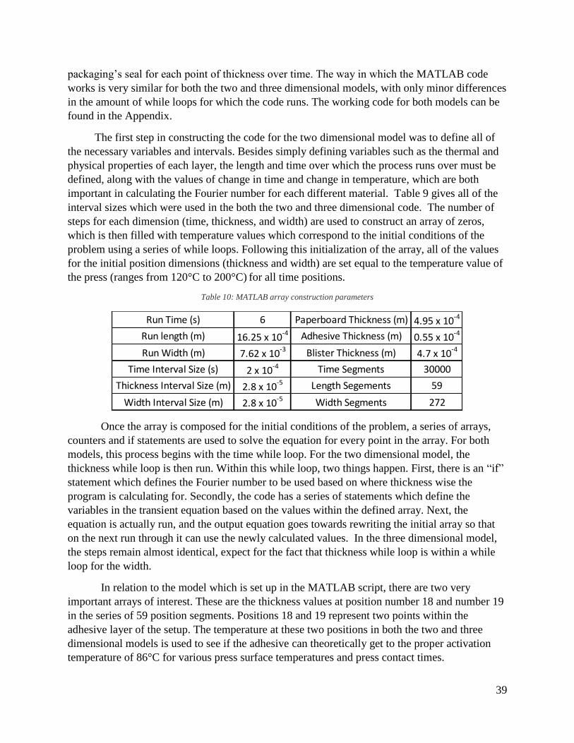
39
packaging’s seal for each point of thickness over time. The way in which the MATLAB code
works is very similar for both the two and three dimensional models, with only minor differences
in the amount of while loops for which the code runs. The working code for both models can be
found in the Appendix.
The first step in constructing the code for the two dimensional model was to define all of
the necessary variables and intervals. Besides simply defining variables such as the thermal and
physical properties of each layer, the length and time over which the process runs over must be
defined, along with the values of change in time and change in temperature, which are both
important in calculating the Fourier number for each different material. Table 9 gives all of the
interval sizes which were used in the both the two and three dimensional code. The number of
steps for each dimension (time, thickness, and width) are used to construct an array of zeros,
which is then filled with temperature values which correspond to the initial conditions of the
problem using a series of while loops. Following this initialization of the array, all of the values
for the initial position dimensions (thickness and width) are set equal to the temperature value of
the press (ranges from 120°C to 200°C) for all time positions.
Table 10: MATLAB array construction parameters
Once the array is composed for the initial conditions of the problem, a series of arrays,
counters and if statements are used to solve the equation for every point in the array. For both
models, this process begins with the time while loop. For the two dimensional model, the
thickness while loop is then run. Within this while loop, two things happen. First, there is an “if”
statement which defines the Fourier number to be used based on where thickness wise the
program is calculating for. Secondly, the code has a series of statements which define the
variables in the transient equation based on the values within the defined array. Next, the
equation is actually run, and the output equation goes towards rewriting the initial array so that
on the next run through it can use the newly calculated values. In the three dimensional model,
the steps remain almost identical, expect for the fact that thickness while loop is within a while
loop for the width.
In relation to the model which is set up in the MATLAB script, there are two very
important arrays of interest. These are the thickness values at position number 18 and number 19
in the series of 59 position segments. Positions 18 and 19 represent two points within the
adhesive layer of the setup. The temperature at these two positions in both the two and three
dimensional models is used to see if the adhesive can theoretically get to the proper activation
temperature of 86°C for various press surface temperatures and press contact times.
Run Time (s) 6 Paperboard Thickness (m) 4.95 x 10⁻⁴
Run length (m) 16.25 x 10⁻⁴ Adhesive Thickness (m) 0.55 x 10⁻⁴
Run Width (m) 7.62 x 10⁻³ Blister Thickness (m) 4.7 x 10⁻⁴
Time Interval Size (s) 2 x 10⁻⁴ Time Segments 30000
Thickness Interval Size (m) 2.8 x 10⁻⁵ Length Segements 59
Width Interval Size (m) 2.8 x 10⁻⁵ Width Segments 272

40
3.3.1 Two-Dimensional Model
The following graphs are representations of the data gathered from the 2D MATLAB
model for various heat press temperatures (120°C, 160°C, and 200ºC). The script which was
composed is capable of giving the temperature of all 59 thickness points of interest. Figure 24
are the graphs and data for the temperatures of the thickness positions 18 and 19 for all three
press surface temperature values of interest. These values vary by a very small amount, not more
than 2%, between the two-dimensional and three-dimensional models. Figure 24 shows the data
obtained from the three press temperatures over 6 seconds.
(a)
(b)
(c)
Figure 24: Various press surfaces temperatures vs time from the two-dimensional model corresponding to press temperatures of
(a) 120 C, (b) 160 C, (c) 200 C.
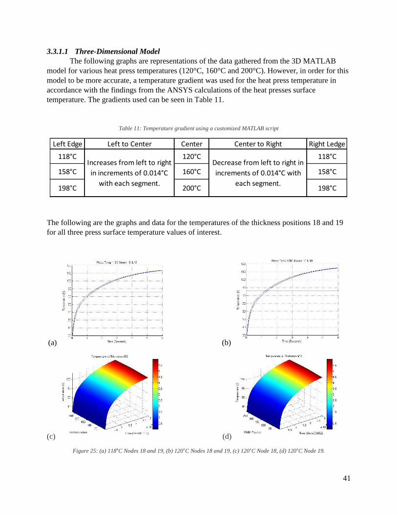
41
3.3.1.1 Three-Dimensional Model
The following graphs are representations of the data gathered from the 3D MATLAB
model for various heat press temperatures (120°C, 160°C and 200°C). However, in order for this
model to be more accurate, a temperature gradient was used for the heat press temperature in
accordance with the findings from the ANSYS calculations of the heat presses surface
temperature. The gradients used can be seen in Table 11.
Table 11: Temperature gradient using a customized MATLAB script
The following are the graphs and data for the temperatures of the thickness positions 18 and 19
for all three press surface temperature values of interest.
(a) (b)
(c) (d)
Figure 25: (a) 118 C Nodes 18 and 19, (b) 120 C Nodes 18 and 19, (c) 120 C Node 18, (d) 120 C Node 19.
Left Edge Left to Center Center Center to Right Right Ledge
118°C 120°C 118°C
158°C 160°C 158°C
198°C 200°C 198°C
Increases from left to right
in increments of 0.014°C
with each segment.
Decrease from left to right in
increments of 0.014°C with
each segment.
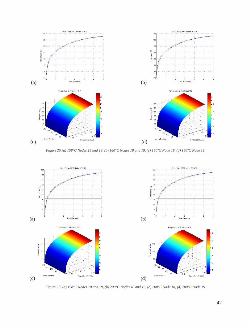
42
(a) (b)
(c) (d)
Figure 26:(a) 158°C Nodes 18 and 19, (b) 160°C Nodes 18 and 19, (c) 160°C Node 18, (d) 160°C Node 19.
(a) (b)
(c) (d)
Figure 27: (a) 198°C Nodes 18 and 19, (b) 200°C Nodes 18 and 19, (c) 200°C Node 18, (d) 200°C Node 19.

43
4 COMPUTATIONAL STUDIES
In addition to the MATLAB program, multiple studies were done in ANSYS to determine
and analyze various conditions, assumptions, and experimental options for the project. ANSYS
was chosen as the program medium for these studies due to the built in ability for SolidWorks
parts to be analyzed by ANSYS. Additionally, the types of studies that were necessary were
highly compatible with the methodology that ANSYS works through.
4.1 STRUCTURAL STUDY The first study performed in ANSYS was the structural study of the press piece and the
different layers of packaging while under pressure. The setup consists of the bottom piece of the
press that comes into contact with the package itself, and three layers of flat material to represent
the paperboard-plastic-paperboard setup of the actual packaging. The bottom paperboard layer
was then fixed and a pressure as applied to the top of the press. The pressure was chosen to by
extrapolating from the recommended process pressure for the adhesive. The pressure range of 40
to 120 pounds per square inch was provided by the Sponsor, and the pressures of 40, 80, and 120
pounds per square inch were chosen to accurately represent the full range. Force values for each
were derived by multiplying these pressure values by the equivalent area of the bottom of the
press, the area that comes into contact with the package. This results in a force value that can be
applied to the top of the press as a uniform load to get the necessary pressure values onto the
three layered sheets representing the package.
(a) (b)
Figure 28: (a) Von-Mises stresses and (b) Strain gradient through the layers of the package.
Error! Reference source not found.29(a) shows the von-Mises stresses located
throughout the package layers while under the pressure of the press. As can be seen, the stresses
are mainly located in the centers of the sides of the contour, with the corners receiving almost no
stress. This means that the corners of the seal might not be experiencing the necessary pressure
for the activation of the adhesive. Another way to look at the situation is to analyze the strain
experienced throughout the package. Error! Reference source not found.29(b) shows the strain
through the package. As can be seen, the strain gradient almost perfectly depicts the outline of
the package. However, just like the stress gradient, the strain is much lower in the corners than

44
the rest of the contour. This combination shows that the seal should theoretically be weaker
along these corners.
4.2 THERMAL STUDIES The bulk of the computational studies performed were thermal studies. While the
MATLAB models were developed mainly to determine the temperatures at different points
within the various layers of the press process, the ANSYS models were designed to validate
experimental designs and procedures, while also validating different assumptions made about the
entire process.
4.2.1 Press Heat Loss Study
In the initial phases of the project, various causes of the inadequate sealing on the
packages were brainstormed and selected for analysis. One such possible cause was convection
heat loss during movement and resting of the press between sealing of the packages. If the press
was losing enough heat between packages it could causes the assumed temperature of the press
to be lower than the temperature needed to accurately seal the packages. Therefore, the first
thermal computational study was one of convection and radiation heat losses in the actual press.
The initial press model was imported directly into ANSYS without any of the
surrounding attachments or packaging equivalents. The initial temperature of the press was set
for 149 Celsius, the mean of the presses effective temperature range. The press was then setup to
experience both convection and radiation heat loss, with the convection coefficient set at 5 watt
per meter squared Kelvin, and an emissivity of 0.1. See section 2.4.3 for an explanation for these
values. The back section of the plate was not given any convection heat transfer due to the fact
that this section of the press would be connected to the other various parts of the system, parts
that have a much larger thermal mass and therefore can be seen as a constant temperature.
Figure 29: Original press heat loss.

45
Figure 29 depicts the final temperature of the press portion of the fixture after the 2.5
second time interval that represents the plate moving to the package. As discussed in the
reasoning of the convection coefficient selection, the press is moving at such a low speed that it
is essentially experiencing free convection. As expected during free convection, the press is
shown to drop by less than a degree over such a short period of time. It is important to note,
however, that such small degree changes might not have any effects on their own, but when
coupled with other alterations such as stress concentrations the compounded conditions could
have a magnified effect causing the package to be inadequately sealed.
4.2.2 Experimental Heating Study
In addition to studying heat loss in the original press, ANSYS was also used to study the
heating procedures for the experimental work that was to be performed to verify the MATLAB
model. This experimental heating study looked at the process of heating up the modified press
design that was to be physically created for testing. The purpose of simulating the heating
process was twofold. First, the simulation could be used to determine how much time is required
to heat the press at a specific power input. Secondly, the simulation could also be used to
determine how much the heat varies along the press surface. This gradient can then be used as
input into the MATLAB model, increasing the accuracy over a simple one dimensional study
where the surface temperature is held constant.
Much like the heat loss study, the press was imported directly from its SolidWorks file
into ANSYS. The press in question was the modified press, specifically designed for the
experimental portion of this project. Section 5.2.1 covers the alterations made to the original
press to get this new design. Once imported, the same heat loss parameters from the previous
study were applied to the modified press. Since the modified press was made from the same
materials and the experimental setup would mirror the typical environment during processing,
the press will experience these same heat losses as it is heating. However, instead of focusing on
the heat loss in the press, this study looks to determine how long it will take to reach the
necessary temperature and under what gradient the modified press will experience after heating.
To that effect, a heat flux was placed applied to designated holes in the press. This heat flux
represents the heating provided by cartridge heaters which will be placed into the modified press
during testing, all four of which are rated for 325 Watts. Additionally, the initial temperature of
the press is set to room temperature, as the press will be heating up from an ambient state. The
resulting heat map after 25 minutes can be seen in Figure 30.

46
Figure 30: Temperature gradient of press after 25 min.
As seen above in Figure 30, the press reaches an average temperature of around 204°C
after heating from room temperature for 25 minutes. 200°C is the highest required press
temperature for the experimental procedure, therefore this confirms the ability of the heaters to
reach the necessary temperature in a reasonable amount of time. Furthermore, it is also possible
to see from a temperature vs time graph how much time would be needed for intermediary
temperatures that will also be used during testing. As noted in Figure 31 the temperature follows
a slight curve over time, and will reach the lower end temperature of 120°C in around 15
minutes.
Figure 31: Maximum press temperature vs time for the press via ANSYS.

47
Finally, the second important aspect of this thermal analysis is to determine the
temperature gradient of the press’s bottom surface. These temperatures are used as a baseline
temperature variation for the two dimensional MATLAB examination. Looking at the same
parameters as before, the temperature gradient shown in Figure 32 was produced. It is important
to note that the variation in temperature of the surface of the press is largely insignificant, on the
order of two degrees Celsius. While not perfectly uniform, this shows that the package should
receive relatively similar temperatures at all areas of the seal. Furthermore, the temperature does
not vary with the width of the contact area, the only variance occurs slightly around the middle
portions of the contour.
Figure 32: Temperature gradient of bottom of press.
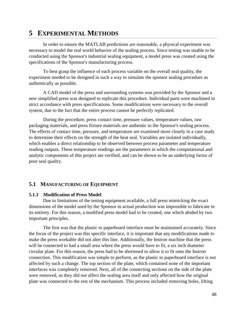
48
5 EXPERIMENTAL METHODS
In order to ensure the MATLAB predictions are reasonable, a physical experiment was
necessary to model the real world behavior of the sealing process. Since testing was unable to be
conducted using the Sponsor's industrial sealing equipment, a model press was created using the
specifications of the Sponsor's manufacturing process.
To best grasp the influence of each process variable on the overall seal quality, the
experiment needed to be designed in such a way to simulate the sponsor sealing procedure as
authentically as possible.
A CAD model of the press and surrounding systems was provided by the Sponsor and a
new simplified press was designed to replicate this procedure. Individual parts were machined in
strict accordance with press specifications. Some modifications were necessary to the overall
system, due to the fact that the entire process cannot be perfectly replicated.
During the procedure, press contact time, pressure values, temperature values, raw
packaging materials, and press fixture materials are authentic to the Sponsor's sealing process.
The effects of contact time, pressure, and temperature are examined more closely in a case study
to determine their effects on the strength of the heat seal. Variables are isolated individually,
which enables a direct relationship to be observed between process parameter and temperature
reading outputs. These temperature readings are the parameters in which the computational and
analytic components of this project are verified, and can be shown to be an underlying factor of
poor seal quality.
5.1 MANUFACTURING OF EQUIPMENT
5.1.1 Modification of Press Model
Due to limitations of the testing equipment available, a full press mimicking the exact
dimensions of the model used by the Sponsor in actual production was impossible to fabricate in
its entirety. For this reason, a modified press model had to be created, one which abided by two
important principles.
The first was that the plastic to paperboard interface must be maintained accurately. Since
the focus of the project was this specific interface, it is important that any modifications made to
make the press workable did not alter this line. Additionally, the Instron machine that the press
will be connected to had a small area where the press would have to fit, a six inch diameter
circular plate. For this reason, the press had to be shortened to allow it to fit onto the Instron
connection. This modification was simple to perform, as the plastic to paperboard interface is not
affected by such a change. The top section of the plate, which contained none of the important
interfaces was completely removed. Next, all of the connecting sections on the side of the plate
were removed, as they did not affect the sealing area itself and only affected how the original
plate was connected to the rest of the mechanism. This process included removing holes, lifting

49
up the side walls, and extruding out the indents into the side of the press. To make the press
attachable to the Instron two holes were added to the center of the press for screws to be inserted
into the Instron’s plate. These holes are directly in the main pocket area above the bubble, and as
such have no real effect on the actual sealing area of the press. Finally, to help the Instron make
accurate passes each time it moves the press down, guiding pin holes were added to the press
itself. These pins would be located on the die which rests on the bottom section of the Instron
and holds the actual package itself. The purpose of these pins to insure that the press always
comes into contact with at the correct interface accurately every time it presses.
Figure 33: The modified press (left) next to the initial press design (right). The blue highlighted section represents the plastic to
paperboard interface that is the focus of the experiments.
The second principle that must be followed is that the press itself must be self-heating.
Since the full press used by the Sponsor was attached to a large machine mechanism that
provided heating, it was not required that the press itself produce heat as it was heated by the
large sections it was connected to. Since the full setup was unable to be replicated in the testing
environment, the press was modified to allow cartridge heaters to be inserted into the upper
portion above the seal area. The thickness of the press was increased to accommodate these
cartridge heaters. In both the original design and the modified press, the plastic to paperboard
interface surface receives heat through conduction through the press itself. Therefore, it does not
matter to the surface whether the heat originates through cartridges, as in the modified press, or
through further conduction to a hot surface above the entire press, as in the original press.

50
Figure 34: The entire modified press, including the holes allowing for the cartridge heater inserts. The important surface
interface is highlighted in blue.
5.1.2 Fabrication of Testing Rig
Upon the finalization of the press fixtures design in SolidWorks, a method of machining
out the parts had to be chosen. While hand machining methods such as drill presses, band saws,
and hack saws were used for the rough cuts of the stock material, fastener pins, and holes, a
computer numerical control (CNC) machine was used on both the press die and the die block.
These machines allow for the easy and quick machining of the complex contours of the pockets
which normally would not be possible to machine in by hand. CNC machines run on what is
referred to as ‘G-Code’. This code can either be manually input into the machine’s interface by
the operator for simple operations such as facing, or generated using computer aided machining
(CAM) software and uploaded into the machine.
Washburn Shop at WPI provides access to CNC machining, CAM Software, as well as a
fully stocked project work space with a plethora of tools and machines. The CNC machines used
in the Washburn Shops are Haas MiniMills. These MiniMills are compatible with CAM
programs written using ESPRIT, the CAM software made by DP Technologies, which is
available on the computers found in the shops.
The two main parts of the design which were machined using programs designed in
ESPRIT were the press die and the die press, which can be seen in Figure 35. The only two types
of operations which were need to make these parts were simple pocketing and drilling
operations. To create the programs, the SolidWorks models needed to be uploaded into ESPRIT.
Given the advanced features of ESPRIT, all of the operations and paths of work were able to be
defined using the smart pocketing and auto chain features. The following is a table of operations
which were used on the parts and which tools were used:

51
Table 12: List of operations and tools
Figure 35: CAD drawings of cutouts.
(a) (b)
Figure 36: (a) Machined press surface, (b) Press and base attached to Instron load frame.
1 Pocketing 3/8 Endmill
2 Pocketing 3/8 Endmill
3 Pocketing 3/8 Endmill
4 Drilling 1/4 Drill Bit
5 Pocketing 3/8 Endmill
6 Drilling 1/4 drill bit

52
5.2 CASE STUDIES
The experimental design will need to reflect the range of process variables as provided by
the Sponsor. To see more clearly the effect each parameter (temperature, pressure, and time) has
on the outcome of the seal, a series of case studies will be performed.
5.2.1 Devices Used for Experiment
4 Watt-Flex Cartridge Heaters: ½ in x 4 ½ in, 325 W, 120 Volts, Cool Tip, 12” standard
leads, 2” cold ends
Cartridge heaters are used to heat the aluminum block to the temperature specified in
each test case. Cartridge heaters are typically tubular in shape, and rely on electrical
resistance to heat substances.
1 Sheet Flexible Composite Mica: 2ft x 2ft, 1mm thickness
Flexible composite Mica is used to insulate the top of the heat sealing press.
Reduction of radiation and free convection both simulates the Sponsor’s heat sealing press
but also allows for a more consistent temperature of the press. Flexible mica is generally
easier to use with this application, especially with its small thickness. The Flexible
Composite Mica is a silicone Mica laminate, and exhibits high flexibility and formability
during set up at room temperature.
1 K-type Thermocouple wire for Al block
Thermocouples are sensors that measure temperature simply made from dissimilar
metals that are joined together at the sensing end, or cold junction compensation end.
Changes in temperatures are read by the sensor as millivolts between the two ends of the
sensor. Different types of thermocouples use different ratios and types of metals for various
applications.
1 K-type Thermocouple wire (sheathed)
Sheathed thermocouples are thermocouple wires surrounded by an insulated material.
Sheathed thermocouples are typically more able to withstand applications that include high
pressures, high temperatures and cycles of vibration.
1 18in x 18in 6061 Aluminum Plate, and 1.5in x 1.5in x 12in 6061 Aluminum Plates
Aluminum was used for the body of the press and die base. It is a solid yet light
weight alloy with exceptional thermal conductivity that will stand up to the pressure put on it
while efficiently transferring heat to the seal.

53
3 .002 in x 1 ft x 1 ft Virgin PTFE Film (MSC Industrial Supply)
o 4 6ft Rolls of PTFE (Virgin) Thickness (Decimal Inch, .0020in)
The Sponsor would have another layer of paperboard that the adhesive would be
sealing to, however since only the seal between plastic and paperboard and not paperboard to
paperboard will be considered, this sheet of Teflon will be used as a non-adhesive layer to
prevent the adhesive from sticking to the lower die base. PTFE Grade 400 typically has a
melting point of 327-335 C, a great deal higher than the temperature range for the project, so
this film was a suitable fit.
Temperature Controller Box with Ceramic Thermocouple
The temperature controller box can measure very high temperatures up for 2300 F,
and is used as a feedback loop to control the temperature to the cartridge heaters.
Digi-Sense Calibrated Dual Laser Infrared Thermometer: Type K, 12:1 ratio
Infrared thermometer calculate temperatures from thermal radiation emitted by the
body being measured. Infrared thermometers are most accurate when comparing
temperatures that are not ambient, and where there is a significant difference in temperatures.
Portable Thermometer/Data Loggers with SD Card and Thermocouple Input
The data loggers are battery powered and can sample, process, and display
measurements without being connected to a computer. The data loggers contain a real time
data recorder, and save the 12-channels temperatures measurements from the thermocouples
into the SD memory card. The data from the memory card can then be downloaded into
Microsoft Excel for further usage and analysis.
5.2.2 Experimental Procedure Overview:
For this procedure, the impact each change in the design variables had on the heat sealing
process as a whole was exploded.
The procedure will be described in greater depth in sections below, but the press will be
heated to temperatures varying from 120 C to 200 C (248 F to 392 F) as suggested by the
Sponsor. The time of seal contact ranges from 1 second to 6 seconds. Lastly, the pressure the
stack of raw packaging materials will be subject to will range from 40 psi to 120 psi.
These case studies are essential to the experimental portion of the project. This testing
set-up isolates single variables at a time. It allows for trends to be observation within temperature
ranges, and amongst pressures, and with changes in time -- this information is vital for the
project deliverable that is to model the relationship between these variables. This information
will be used in conjunction with the analytical and computational models, but this is particularly
insightful because this should be very close to how the Sponsor performs their heat seals.

54
The case studies can be summarized as follows:
1. 3 Temperatures: 120 C, 160 C, 200 C
2. 3 Pressures: 40 psi (727.2 lbf), 80 psi (1454.4 lbf), 120 psi (2181.6 lbf)
3. 4 Press Contact Times: 1 sec, 2 sec, 4 sec, 6 sec
The experimental trials are summarized in Table 13.
Table 13: Trial runs for all temperature, time and pressure parameters
Cartridge heaters will allow for the press to attain the range of temperatures detailed
above and a controller will vary and regulate the power input to the cartridges to ensure a proper
press temperature. With the use of experimental equipment, temperature changes of predefined
positions of each layer will be recorded as the experiment proceeds. These temperature changes
will be then compared to the computational model for accuracy validation of the latter. A more
detailed experimental methodology is described in the next section.
5.2.3 Detailed Experimental Procedure
5.2.3.1 Experimental Setup
1. Attach 2 layers of flexible mica on top of press, and secure for proper insulation.
2. Attach top of press to Instron machine using two screws, and insert the long pins in the
die base into the holes in the press in order to align the base and press.
3. Remove long alignment pins in die base and replace with short structural pins.
4. Power on and configure Portable Thermometer with SD Card. This will be used to record
data temperature data throughout experiment.
5. Insert the four cartridge heaters into their specified bores.
a. Plug heater into socket wire in back of controller, turn on power of controller and
adjust for temperature.
120 C Time 1 Time 2 Time 3 Time 4
Pressure 1 1 second, 40 psi 2 seconds, 40 psi 4 seconds, 40 psi 6 seconds, 40 psi
Pressure 2 1 second, 80 psi 2 seconds, 80 psi 4 seconds 80 psi 6 seconds, 80 psi
Pressure 3 1 second, 120 psi 2 seconds, 120 psi 4 seconds, 120 psi 6 seconds, 120 psi
160 C Time 1 Time 2 Time 3 Time 4
Pressure 1 1 second, 40 psi 2 seconds, 40 psi 4 seconds, 40 psi 6 seconds, 40 psi
Pressure 2 1 second, 80 psi 2 seconds, 80 psi 4 seconds 80 psi 6 seconds, 80 psi
Pressure 3 1 second, 120 psi 2 seconds, 120 psi 4 seconds, 120 psi 6 seconds, 120 psi
200 C Time 1 Time 2 Time 3 Time 4
Pressure 1 1 second, 40 psi 2 seconds, 40 psi 4 seconds, 40 psi 6 seconds, 40 psi
Pressure 2 1 second, 80 psi 2 seconds, 80 psi 4 seconds 80 psi 6 seconds, 80 psi
Pressure 3 1 second, 120 psi 2 seconds, 120 psi 4 seconds, 120 psi 6 seconds, 120 psi

55
6. Attach thermocouples below all layers, between sealed layers, above top layer, and
attached to the heated press, and secure with high temperature tape.
7. Begin heating up the press to the specified temperature. The heating should take about
20-25 minutes to reach initial specified temperature. The controller will indicate the
current temperature as well as the desired temperature, and the experiment should
proceed once the set value and the process value match within a range of 1 degree.
8. Carefully place plastic blister into the pocket of the die base then place the paperboard on
top.
9. Begin Instron test cycle.
5.2.3.2 Trial Run Procedure
1. Configure controller to specified temperature.
2. Ensure that thermometer with SD card is working properly and begin recording.
3. Begin running trials at 120 C, then 160 C, and last 200 C. Complete all trials at specific
temperature before moving onto next set of trials.
For the first temperature of 120 C the following trials should include: 40 psi at
1 second, 40 psi at 2 seconds, 40 psi at 4 seconds, 40 psi at 6 seconds, 80 psi at
1 second, 80 psi at 2 seconds, 80 at 4 seconds, 80 psi at 6 seconds, 120 psi at
1 second, 120 psi at 2 seconds, 120 psi at 4 seconds, and 120 psi at 6 seconds.
4. Very gently lift and remove package to not damage any potential seals.
5. After each trail run, evaluate the strength of the seal.
Comments that include how difficult it was to remove the seal and if there were
any noticeable differences in seal strength along the length of the seal should be
noted.
6. Repeat previous set-up instructions for inserting next plastic and paperboard.
At the end of the cycle, heat the press to the next temperature.

56
6 RESULTS AND DISCUSSION
Throughout the duration of the heat seal simulation, thermocouples were used to measure
the temperature of the important layers during the sealing process. These thermocouples were
placed strategically on top of the paperboard and between the plastic blister, representing the
adhesive layers that is expected to melt to create the seal. These values will be obtained for each
of the 36 trials as described previously.
The temperature values received from these devices for each case study should give way
towards experimental conclusions in regards to the effects of the process parameters as it relates
to seal strength. This experimental component should also be able to verify the analytical
procedure for predicting the temperature values for the adhesive layer.
6.1 VALIDATION OF MATLAB PREDICTIONS Upon completion of the experimental portion of the project, some discrepancies between
the heat transfer data generated from the MATLAB scripts and the temperature data which was
collected from the sealing runs were noticed. However, after further investigation, it appeared
that these differences between the theoretical MATLAB values and the experimental were easily
calculated and showed that the experimental temperature values difference from the theoretical
values was consistent amongst specific temperature and time values. Temperatures recorded
during the experimental runs were for at the adhesive paperboard interface, so the temperatures
from position node 18 of the three dimensional MATLAB script were used for the comparisons.
𝑇𝑇ℎ𝑒𝑜𝑟𝑒𝑡𝑖𝑐𝑎𝑙 − 𝑇𝐸𝑥𝑝𝑒𝑟𝑖𝑚𝑒𝑛𝑡𝑎𝑙
𝑇𝑇ℎ𝑒𝑜𝑟𝑒𝑡𝑖𝑐𝑎𝑙× 100 = 𝑑𝑖𝑓𝑓𝑒𝑟𝑒𝑛𝑐𝑒 (%)
Equation 15: Percent difference formula.

57
(a) (d)
(b) (e)
(c) (f)
(g)
Figure 37: Plots of various surface temperatures for both MATLAB and experimental trials and a plot of percent differences for
all surface temperatures. (a) MATLAB 120 C, (b) MATLAB 160 C, (c) MATLAB 200 C, (d) experimental 120 C,
(e) experimental 160 C, (f) experimental 200 C, (g) plot of percent differences.

58
The percent difference between the theoretical and experimental values was calculated by
using Figure 39. This equation works by first subtracting the experimental temperature from the
theoretical temperature, followed by dividing this subtraction by the theoretical temperature, and
then finally multiplying by one-hundred. The output of this equation is the percentage by which
the temperature of the experimental values are off from the theoretical temperature values.
Figure 39 lays out the results generated from using Equation 15. Table 15 gives an example of
one of the calculations which was used for calculating the percent difference for a specific point.
In order to compensate for the fact that the MATLAB calculations do not take into account the
pressure of the press on the packaging, the three recorded experimental temperatures for any
given set of temperature and time values were averaged and used in the calculations for the
percent difference. An example of this averaging is that the experimental temperature for 120 C
press temp and 1 second of contact was the average of the temperatures for the 40 psi, 80 psi,
and 120 psi runs, which were 51.2 C, 51.2 C, and 55.9 C
Table 14: Values of percent differences for various press surface temperatures
As seen in Figure 36 and Table 14, there is an average of 40% difference between the
results of the MATLAB script and the data collected experimentally. These differences between
the experimental and theoretical values are very much understandable in this situation. The
equation which was used in the MATLAB was for understanding the general workings of the
heat transfer and did not have any means of compensating for any factors that may have affected
the heat transfer except for the thermal conductivity/resistivity of each layer. Compared to an
ideal case such as that of the MATLAB script, the real life process has many variables which
could potentially effect the heat transfer through the packaging. This difference can be explained
using the concept of contact resistance, which was discussed earlier on in the report within the
conductive heat transfer section. With further research and experimentation, values for the
Run
120 C Theoretical Temperature (°C) Experiemental Temperature (°C) Percent Difference Time (sec)
82.288 52.7667 35.87558332 1
95.3746 60.1667 36.91538418 2
109.1619 66.2 39.35613066 4
115.1076 69 40.05608665 6
160°C
105.5773 68.5667 35.05545226 1
124.5084 77.6667 37.62131712 2
144.466 87.2 39.63977683 4
153.0776 88.1333 42.42573701 6
200°C
128.8665 80.6 37.45465268 1
153.6422 93.8667 38.90565222 2
179.7702 101.9 43.31652298 4
191.0477 103.9 45.61567609 6

59
contact resistances can be calculated and applied to the equation for heat transfer in the form of
extra resistivity values. An example of this modified equation can be found in Equation 15.
𝑄 =∆𝑇
∑ 𝑅=
∆𝑇
𝑅𝑃𝑎𝑝𝑒𝑟 + 𝑅𝑐𝑜𝑛𝑡𝑎𝑐𝑡(𝑃𝑎𝑝𝑒𝑟−𝐴𝑑ℎ𝑒𝑠𝑖𝑣𝑒) + 𝑅𝐴𝑑ℎ𝑒𝑠𝑖𝑣𝑒 + 𝑅𝑐𝑜𝑛𝑡𝑎𝑐𝑡(𝐴𝑑ℎ𝑒𝑠𝑖𝑣𝑒−𝑃𝑙𝑎𝑠𝑡𝑖𝑐) + 𝑅𝑃𝑙𝑎𝑠𝑡𝑖𝑐
Equation 16. A modified version of the steady state resistance equivalence that accounts for contact resistance between layers.
6.2 DEVELOPMENT OF SEAL QUALITY SCALE In addition to validating the developed MATLAB program, the results from the
experimental work can be used to develop a seal quality index that can take input in the form of
the three process parameters, temperature, time, and pressure, and produce an approximate grade
for the strength of the seal.
6.2.1 Subjective Quantification
The procedure for seal quality evaluation begins with the identification and categorization
of 3 levels of seal quality. These ratings are based on the end-result of the cardboard after a
sealing attempt has been made. The lowest seal rating is 0 – this is denoted with a lack of
cardboard deformation. Seal areas rated a level 0 would have no visual difference between areas
of the cardboard that made no contact with the press whatsoever. Areas with a rating of level 2
have a very clear, thin, smooth layer that follows the area of the press contour. Level 1 denotes a
seal quality that is between levels 0 and 2. In level 1, there is very slight press indentation, and
there is a noticeable shimmer in the contour when light is reflected off of it. There are speckles in
the semi-clear contour outline. Since there are only three distinct and observable levels of seal
quality to the human eye, a rule of the thumb was developed where any area of the contour that
was not designated a level 0 or a level 2 would be labelled a level 1. The reasoning was due to
the fact that both level 0 and level 2 were easily discernable to the human eye, while level 1 was
harder to recognize. Figure 38 displays the three levels.
(a) (b) (c)
Figure 38. The three levels shown in a seal: (a) Level 0, (b) Level 1, and (c) Level 2.
After a consensus on the definition of each of the seal quality levels, multiple individuals
observed the seals and recorded values for the areas of each leveling of sealing. These areas were
compared between observers and an average value for each area was obtained.

60
6.2.2 Optical Quantification and Analysis
To help improve the accuracy of the previous subjective observations, an optical
quantification was performed to provide exact area percentages for the levels. Each of the three
levels were designated a different color, and the actual seals were colored according to their
designation. These seals were then observed using an image analysis software, which quantifies
the exact level of each color. Figure 39 is an example of a seal after image analysis. The outputs
of the image analysis software are area values in percentages, one seal was chosen to be the
standard size to which all other areas could be compared. For this purpose, the seal created
during trial 36, the highest of all three parameters, was chosen due to it containing a near 100%
level 2 seal. The area determined from this seal was used as the base area and there all other area
values were converted to percentages of this base area.
(a) (b)
Figure 39: (a) Example of colored seal, (b) An example of the seal are analysis performed under the image analyzing equipment.
In addition to providing exact values for the area percentages of each seal, a microscope
was used to detail the different levels on a microstructure level. As can be seen in Figure 40, the
difference between levels 1 and 2 were drastic, while the difference between levels 0 and 1 were
less pronounced. This dramatic difference lead to the determination that the level 2 seal was
fundamentally significant compared to the other two levels. For this reason, the area values for
level 2 would be the largest weighted factor when determining the quality of a seal.

61
Figure 40. The macro and microscopic views of the three different seal levels.
6.2.3 Determination of Seal Quality Scale
Once objective quantification of the areas of each level was achieved a seal quality scale
could be developed. This quality scale would later be used to as part of a larger seal strength
equation that could predict the seal quality of a process with specific temperature, dwell time,
and press inputs. The quality scale will assign a value to each trial run numbering 1 through 5,
with 1 being the lowest quality or “no effect” case, and 5 being the strongest seal created in the
trials.
The quality values themselves were assigned to each trial using a combination of the
areas of each level of seal discussed in the previous section. From the optical observations
performed on a microscopic scale, it was shown that the structure of a level 2 area was
drastically evolved compared to the level 1 structure. Additionally, the level 1 case showed no
large difference over a level 0. For this reason, the level 2 area values were weighted to a much
larger degree than their level 1 counterpart for the process of determining the seal quality scale.
Given these parameters, each trial received a designated seal quality. Each of these qualities
describe an approximation to how well the package had sealed.
Table 15: Specifications of the seal quality index
1 No level 1 or level 2
2 No level 2, less than 50% of total area level 1
3 Less than 25% of total area level 2
4 Between 25 and 50% level 2
5 Over 50% level 2
Seal Quality Index
These can be extrapolated for any combination
Level 0
Level 2
Level1

62
Table 16: The seal quality and process parameters of each experimental run
Run # Time (s) Temperature (°C) Pressure (psi) Strength Rating
1 1 1
2 2 1
3 4 1
4 6 1
5 1 1
6 2 1
7 4 2
8 6 2
9 1 1
10 2 2
11 4 2
12 6 2
13 1 2
14 2 2
15 4 2
16 6 3
17 1 1
18 2 2
19 4 3
20 6 4
21 1 2
22 2 3
23 4 4
24 6 4
25 1 2
26 2 3
27 4 4
28 6 5
29 1 2
30 2 4
31 4 5
32 6 5
33 1 3
34 2 5
35 4 5
36 6 5
80
120
120
160
200
40
80
120
40
80
120
40

63
6.3 SEAL STRENGTH QUALITY EQUATION Once each seal acquired a specified strength quantity, an equation could be developed to
predict these strength values based on the various process parameters. The three process
parameters of this specific sealing operation were pressure, time, and temperature. Each of these
parameters will have different effectiveness on increasing the quality of the total seal strength.
The developed equation will need to reflect these levels of effectiveness for the different process
parameters, and will need to express the value of each on a similar level of magnitude.
To begin the development of this equation, the three process parameters were plotted
individually against the steal strength of each experimental run. This plot allows the visualization
of the correlation between each of these process parameters and the strength of the seal. As can
be seen in the following plots, and increase in each process parameter reflected an increase in the
effective strength of each seal. However, the pressure parameter had the lowest effect, to the
point that increasing the pressure resulted in no valuable increase in strength of the seal. The
time parameter had a slightly larger effect, while the temperature had a much larger effect than
either of the other parameters. This will result in temperature having the largest weight in any
quality prediction equation.
(a) (b)
(c)
Figure 41: (a) Pressure versus seal quality, (b) Time versus seal quality, (c) Temperature versus seal quality.

64
With these correlations between the individual process parameters and the strength of the
seal, an equation could be formed. The final equation can be seen in Equation 17.
1 + 4 [𝑅𝑃
2
Σ𝑅𝑃2 (
𝑃−𝑃𝑚𝑖𝑛
𝑃𝑚𝑎𝑥−𝑃𝑚𝑖𝑛) +
𝑅𝑡2
Σ𝑅𝑡2 (
𝑡−𝑡𝑚𝑖𝑛
𝑡𝑚𝑎𝑥−𝑡𝑚𝑖𝑛) +
𝑅𝑇2
Σ𝑅𝑇2 (
𝑇−𝑇𝑚𝑖𝑛
𝑇𝑚𝑎𝑥−𝑇𝑚𝑖𝑛)]= 𝑆𝑒𝑎𝑙 𝑄𝑢𝑎𝑙𝑖𝑡𝑦
Equation 17: Equation for seal quality prediction.
The three colored weighting factors in Equation 17 represent the effect that each process
parameter has on the seal strength. These weighting factors are the correlation between these
parameters divided by the total correlation of all process parameters, forming a fraction of the
individual parameter to the total of all three parameters. Next, the input process parameters of
pressure, time, and temperature are converted to ratios between the minimum and maximum
values. This conversion is necessary to get each of the process parameters to the same
magnitude, since temperature and pressure are often two magnitudes larger than the time. These
maximum and minimum values are entirely determined by the specific process being studied.
Finally, the result thus far will be a value between 0 and 1, which allows further conversion to
the scale previously used between 1 and 5. Future extrapolation for any heat sealing process can
be further adapted to the desired process by changing the conversion to any scale, such as 1 to 10
or 1 to 100.

65
7 CONCLUSIONS AND FUTURE WORK
The group was able to successfully utilize computational, analytical and experimental
procedures to help verify the fundamental heat transfer relationships at play in the heat sealing. First,
analytical relationships were utilized to estimate key values for the adhesive layer under various
process conditions. The use of MATLAB provided concrete evidence for a few important trends. The
first trend is an observation that suggests the temperatures of the system changed more initially, and
then that temperature change decreased slightly as time elapsed. According to the data collection
through the theoretical model that MATLAB presented, every package whose process parameters
were examined should have sealed. However, this is not accurate as compared the experimental
results that state that at lower temperature values, the packages do not seal. Overall though, the
computational MATLAB model proved to be very precise when predicting the expected temperature
values. However, in the experimental portion of the projects the trials consistently produced results
40% less than the anticipated values. Though these results are inaccurate, they show that the
MATLAB code can consistently solve for a temperature, across all process parameters. After this
data was obtained and considered, steps were taken to correlate the process parameters with a
quantifiable means of measuring heat seal quality. Seal quality was differentiated based on team-
innovated observational analysis and these varying levels of sealing were given a value ranging from
0 to 2. For each trial, the various seal levels were designated a different color and the actual contact
areas were colored according to their designation. Optical quantification provided the percentages of
each seal level. These steps provided data that when combined and manipulated, yielded a predictive
function capable of correlating input process parameters to an output seal quality rating. This
overarching equation is capable of delivering an accurate seal quality prediction. It is recommended
to use this process in conjunction with another supplementary equation that has been developed that
takes the output quality rating as output by the first equation and standardizes it on a scale of 1 to 5.
The group recommends that future work be done to further understand thermal contact
resistance and its role in the consistent percentage error found in the predicted results. A simple
visualization of where the contact resistance would appear can be seen in Equation 16. However, this
equation only applies to simple steady state situations, so further work will need to be done to
extrapolate this into a transient system. Additionally, to further optimize the heat sealing process of
the Sponsor’s packaging, research could be performed to test other material choices and heat transfer
alternatives that may require less energy input in the sealing process to enhance further cost
effectiveness throughout the manufacturing procedure. In the predictive seal quality equation, far
more trials are recommended to make the presented correlation as accurate as possible. The group
would like to note that with the implementation of material choice/heat transfer mode alternatives,
the predictive quality equation may change, but a methodology similar to the one presented in this
project would prove useful to develop this new relationship.

66
8 BIBLIOGRAPHY
1. Kalpakjian, Serope, and Steven R. Schmid. Manufacturing Engineering and Technology.
7th ed. Boston: Pearson, 2006. Print.
2. "Blister cards." Ecobliss. Ecobliss, n.d. Web.
3. "Blister Machine FAQ." The Differences Between Thermoforming and Cold Forming
Blister Pack. Jornen Machinery Co., Ltd., n.d. Web.
4. "Technologies." Ecobliss. Ecobliss, n.d. Web.
5. Bergman, Theodore L., Adrienne S. Lavine, Frank P. Incropera, and David P. Dewitt.
Fundamentals of Heat and Mass Transfer. 7th ed. Jefferson City: John Wiley and Sons,
2011. Print.
6. Calhoun, Allison R., and Jerry Golmanavich. Plastics Technician's Toolbox. Brookfield,
Ct: Society of Plastics Engineers, 2002. Print.
7. Hishinuma, Kazuo. Heat Sealing Technology and Engineering for Packaging: Principles
and Applications. Lancaster, PA: DEStech Publications, 2009. Print.
8. Bergman, T., Lavine, A., Incropera, F., & Dewitt, D. (n.d.). The Heat Diffusion Equation.
In -Introduction to Heat Transfer. 6th ed. 2011: John Wiley & Sons.
9. "Aerospace Specification Metals Inc." Aluminum 6061-T6; 6061-T651. ASM, n.d. Web.
10. Aluminum Tempers, Specification and Designations." Engineers Edge. Engineers Edge.
Web. 26 Apr. 2015. <http://www.engineersedge.com/aluminum_tempers.htm>.
11. Pavlina, E.j., and C.j. Tyne. "Correlation of Yield Strength and Tensile Strength with
Hardness for Steels." Journal of Materials Engineering and Performance 17.6: 888-93.
Springer Link. Web. 26 Apr. 2015. <http://link.springer.com/article/10.1007/s11665-008-
9225-5.
12. Hardenable Alloy Steels." Total Materia. Key to Metals AG, 2 Nov. 2002. Web. 26 Apr.
2015.
<http://www.totalmateria.com/page.aspx?ID=CheckArticle&LN=EN&site=kts&NM=91
13. Callister, William, and David Rethwisch. Fundamentals of Materials Science and
Engineering. Vol. 4. John Wiley & Sons, 2012. Print.
14. Dossett, Jon, and Howard Boyer. Practical Heat Treating. 2nd ed. ASM International,
2006. Print.
15. Sanders, Robert E. "Technology Innovation in Aluminum Products." JOM 53.2: 21-
25.Springer Link. Web. 26 Apr. 2015. http://link.springer.com/article/10.1007/s11837-
001-0115-7.

67
16. Understanding Weld Resistance. Digital image. Resistance Welding Equiprment and
Supplies. SpotWedling Consultants, Inc., n.d. Web.
17. Williamson, M., and A. Majumdar. "Effect of Surface Deformations on Contact
Conductance." Heat Transfer 114 (1992): ASME DC. 23 May 2008. Web. 26 Feb. 2015.
18. Shields, J. Adhesives Handbook. London: Butterworths, 1984. Print.
19. ASTM F3004-13e1, Standard Test Method for Evaluation of Seal Quality and Integrity
Using Airborne Ultrasound, ASTM International, West Conshohocken, PA,
2013, www.astm.org.
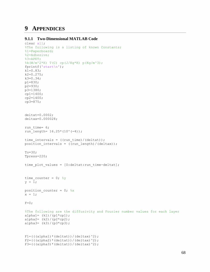
68
9 APPENDICES
9.1.1 Two-Dimensional MATLAB Code clear all; %The following is a listing of known Constants; %1=Paperboard; %2=Adhesive; %3=APET; %k(W/m^2*K) T(C) cp(J/Kg*K) p(Kg/m^3); fprintf('start\n'); k1=0.83; k2=0.275; k3=0.34; p1=830; p2=930; p3=1380; cp1=1400; cp2=1400; cp3=875;
deltat=0.0002; deltax=0.000028;
run_time= 6; run_length= 16.25*(10^(-4));
time_intervals = ((run_time)/(deltat)); position_intervals = ((run_length)/(deltax));
To=30; Tpress=220;
time_plot_values = [0:deltat:run_time-deltat];
time_counter = 0; %y y = 1;
position_counter = 0; %x x = 1;
F=0;
%The following are the diffusivity and Fourier number values for each layer alpha1= (k1)/(p1*cp1); alpha2= (k2)/(p2*cp2); alpha3= (k3)/(p3*cp3);
F1=(((alpha1)*(deltat))/(deltax)^2); F2=(((alpha2)*(deltat))/(deltax)^2); F3=(((alpha3)*(deltat))/(deltax)^2);

69
temperature_array = zeros(2500, 59); % make 15x12500 array of all zeros fprintf('starting zeros\n'); temp_counter = 1; temp2_counter = 1;
while (temp_counter <=2500) while (temp2_counter<=59)
temperature_array(temp_counter,temp2_counter)=To; temp2_counter= temp2_counter +1; end temp2_counter =1; temp_counter= temp_counter+1; end
temp_counter=1;
while (temp_counter <= 2500) temperature_array(temp_counter, 1) = Tpress; % set all columns to 204.444 temp_counter = temp_counter + 1; end fprintf('done x\n'); temp_counter = 1;
while (temp_counter <= 59) temperature_array(1,temp_counter) = To; % set all rows to 30 temp_counter = temp_counter + 1; end
temperature_array(1,1) = Tpress; % fix top left cell fprintf('done with initialization\n');
fprintf('1,2 = %d\n', temperature_array(1,2));
while time_counter <(run_time-deltat) %Time Loop
x=1; y = y + 1; %Defining y position of temperature array position_counter = 0; time_counter = time_counter+deltat;
while position_counter <=(run_length-deltax) %Position Loop
x= x+1; position_counter = position_counter+deltax;
if (position_counter == 4.95*(10^(-4))) F= ((F1+F2)/2); elseif (position_counter== 5.5*(10^(-4))) F=((F2+F3)/2); elseif (position_counter== 10.2*(10^(-4)))

70
F=((F2+F3)/2); elseif (position_counter==10.75*(10^(-4))) F=((F1+F2)/2); elseif (position_counter < (4.95*(10^-4)) && (position_counter > 0)) F=F1; elseif (position_counter < (5.5*(10^(-4))) && position_counter >
(4.95*(10^-4))) F=F2; elseif (position_counter < (10.2*(10^(-4))) && position_counter >
(5.5*(10^(-4)))) F=F3; elseif (position_counter < (10.75*(10^(-4))) && position_counter
>(10.2*(10^(-4)))) F=F2; elseif (position_counter <(16.25*(10^(-4))) && position_counter >
(10.75*(10^(-4)))) F=F1;
else
F=F1;
end
if ((x+1) > position_intervals) Tafter=Tmiddle; else Tafter = temperature_array(y-1,x+1); end
Tbefore = temperature_array(y-1,x-1); Tmiddle= temperature_array(y-1,x); temperature_array(y,x) = ((Tafter + Tbefore)*F)+ ((1-(2*F))*Tmiddle);
if (x == 2 && y == 2) fprintf('Tafter = %d, Tbefore = %d, Tmiddle = %d, F
= %d\n',Tafter,Tbefore,Tmiddle,F); fprintf('Coordinates = (%d, %d), Value = %d\n', x,y,((Tafter +
Tbefore)*F)+ ((1-(2*F))*Tmiddle)); end
end end
plot_counter = 0; grid on; hold on; title('Temperature vs Time'); xlabel('Time (Seconds)'); ylabel('Temperature (C)'); while plot_counter < position_intervals %position_intervals plot(time_plot_values,temperature_array(:,plot_counter+1));

71
plot_counter = plot_counter+1; end
9.1.2 Three-Dimensional MATLAB Code clear all; %The following is a listing of known Constants; %1=Paperboard; %2=Adhesive; %3=APET; %k(W/m^2*K) T(C) cp(J/Kg*K) p(Kg/m^33); fprintf('start\n'); k1=0.83; k2=0.275; k3=0.34; p1=830; p2=930; p3=1380; cp1=1400; cp2=1400; cp3=875;
deltat=0.0002; deltax=0.000028; deltaw=0.000028; % % run_time= 1; run_length= 16.25*(10^(-4)); run_width=0.00762; % % time_intervals = ((run_time)/(deltat)); position_intervals = ((run_length)/(deltax)); width_intervals = ((run_width)/(deltaw)); % To=30; % Tpress=149; Tpress1=[118:(2/135):120]; Tpress2=120; Tpress3=[120:(-2/135):118]; % time_plot_values = [0:deltat:run_time-deltat];
time_counter = 0; %w w = 1;
position_counter = 0; %y y = 1;
width_counter = 0; %x x=0;

72
F=0;
%The following are the diffusivity and Fourier number values for each layer alpha1= (k1)/(p1*cp1); alpha2= (k2)/(p2*cp2); alpha3= (k3)/(p3*cp3);
F1=(((alpha1)*(deltat))/(deltax)^2); F2=(((alpha2)*(deltat))/(deltax)^2); F3=(((alpha3)*(deltat))/(deltax)^2);
temperature_array = zeros(59, 272,5000); % make 2000x2000x2000 array of all
zeros fprintf('starting zeros\n');
temp_counter = 1; temp2_counter = 1; temp3_counter = 1;
while (temp_counter <= 59) while (temp2_counter <=272) while(temp3_counter <=5000) temperature_array(temp_counter,temp2_counter,temp3_counter) = 30; temp3_counter= temp3_counter + 1; end temp3_counter=1; temp2_counter=temp2_counter+1; end temp2_counter=1; temp_counter= temp_counter +1; end
fprintf('done x\n'); temp_counter = 1; temp2_counter =1;
%135 is Tpress1 %136 is Tpress %137 is Tpress2 while (temp_counter <=136) temperature_array(1,temp_counter,1:5000)=Tpress1(temp_counter); temp_counter= temp_counter +1; end temperature_array(1,136,1:5000)=Tpress2;
while (temp2_counter <=136) temperature_array(1,136+temp2_counter,1:5000)=Tpress3(temp2_counter); temp2_counter= temp2_counter +1; end

73
fprintf('done with initialization\n');
fprintf('1,2,2 = %d\n', temperature_array(1,2,2));
while time_counter <(run_time-
deltat) %Time Loop % y=1; % x= x+1; x=0; y=1; w = w + 1; %Defining y position of temperature array
width_counter=0; position_counter = 0; time_counter = time_counter+deltat; fprintf( 'time_counter %d\n', time_counter);
while position_counter <=(run_length-deltax) %Position Loop % y=y+1; width_counter=0; x=0; y= y+1; position_counter = position_counter+deltax;
if (position_counter == 4.95*(10^(-4))) F= ((F1+F2)/2); elseif (position_counter== 5.5*(10^(-4))) F=((F2+F3)/2); elseif (position_counter== 10.2*(10^(-4))) F=((F2+F3)/2); elseif (position_counter==10.75*(10^(-4))) F=((F1+F2)/2); elseif (position_counter < (4.95*(10^-4)) && (position_counter > 0)) F=F1;
elseif (position_counter < (5.5*(10^(-4))) && position_counter >
(4.95*(10^-4))) F=F2; elseif (position_counter < (10.2*(10^(-4))) && position_counter >
(5.5*(10^(-4)))) F=F3; elseif (position_counter < (10.75*(10^(-4))) && position_counter
>(10.2*(10^(-4)))) F=F2; elseif (position_counter <(16.25*(10^(-4))) && position_counter >
(10.75*(10^(-4)))) F=F1;
else

74
F=F1;
end
while width_counter <=(run_width-deltaw) %width Loop
x=x+1;
width_counter = width_counter+deltaw;
Tbeforey = temperature_array (y-1,x,w-1);
Tmiddle= temperature_array(y,x,w-1);
if ((y+1) > position_intervals) Taftery=Tmiddle; else Taftery = temperature_array (y+1,x,w-1); end
if((x==1) && (w<1)) Tbeforex= temperature_array(y,x+1,w); Tafterx=temperature_array(y,x+1,w); elseif(x==1) Tbeforex= temperature_array(y,x+1,w-1); Tafterx=temperature_array(y,x+1,w-1); elseif((x+1) > width_intervals) Tafterx = temperature_array(y,x-1,w-1); Tbeforex = temperature_array(y,x-1,w-1); else Tbeforex = temperature_array(y,x-1,w-1); Tafterx= temperature_array(y,x+1,w-1); end
temperature_array(y,x,w) = ((Taftery + Tbeforey + Tafterx +
Tbeforex)*F)+ ((1-(4*F))*Tmiddle);
end end end

75
% grid on; % hold on;
% y=[0:0.000028:0.00762]; % x=[0:0.0002:6]; % % c=meshgrid(x(1:end-1),y(1:end-1)); % % z(:,:)= temperature_array(18,:,:); % % % figure; % surf(z,c); % title('Temperature_array'); % xlabel('elements in x'); % ylabel('elements in y'); % zlabel('elements in z'); % axis tight; % shading interp; % colorbar;
% plot_counter=1; % width_counter=1; % grid on; % hold on; % graph_counter=1; % % % while plot_counter < position_intervals % graph_counter= graph_counter+1; % plot(time_plot_values,
squeeze(temperature_array(plot_counter,136,:))); % plot_counter=plot_counter+1; % end