heat exchanger efficiency - rice university · pdf filecosmosfloworks 2006 tutorial 6-1 6 heat...

COSMOSFloWorks 2006 Tutorial 6-1

6 Heat Exchanger Efficiency

COSMOSFloWorks can be used to study the fluid flow and heat transfer for a wide variety of engineering equipment. In this example we use COSMOSFloWorks to determine the efficiency of a counterflow heat exchanger and to observe the temperature and flow patterns inside of it. With COSMOSFloWorks the determination of heat exchanger efficiency is straightforward and by investigating the flow and temperature patterns, the design engineer can gain insight into the physical processes involved thus giving guidance for improvements to the design.A convenient measure of heat exchanger efficiency is its “effectiveness” in transferring a given amount of heat from one fluid at a high temperature to another fluid at a lower temperature. The effectiveness can be determined if the temperature at all flow openings are known. In COSMOSFloWorks the temperature at the fluid inlets are specified and the temperature at the outlets can be easily determined. Heat exchanger effectiveness is defined as follows:

The actual heat transfer can be calculated as either the energy lost by the hot fluid or the energy gained by the cold fluid. The maximum possible heat transfer is attained if one of the fluids were to undergo a temperature change equal to the maximum temperature difference present in the exchanger, which is the difference in the inlet temperature of the hot and cold fluids respectively . Thus, for a counterflow heat exchanger

the effectiveness is defined as follows: - if hot liquid capacity rate is

less than cold liquid capacity rate - if hot liquid capacity rate is more

than cold liquid capacity rate, where the capacity rate is the product of the mass flow and the specific heat capacity: C= (Ref.2)

The goal of the project is to calculate the effectiveness of the counterflow heat exchanger.

ε actual heat transfermaximum possible heat transfer ------------------------------------------------------------------------------=

Thotinlet Tcold

inlet–( )

εThot

inlet Thotoutlet–

Thotinlet Tcold

inlet–------------------------------------=

εTcold

outlet Tcoldinlet–

Thotinlet Tcold

inlet–------------------------------------=

m· c

Chapter 6 Heat Exchanger Efficiency

6-2

Open the Model

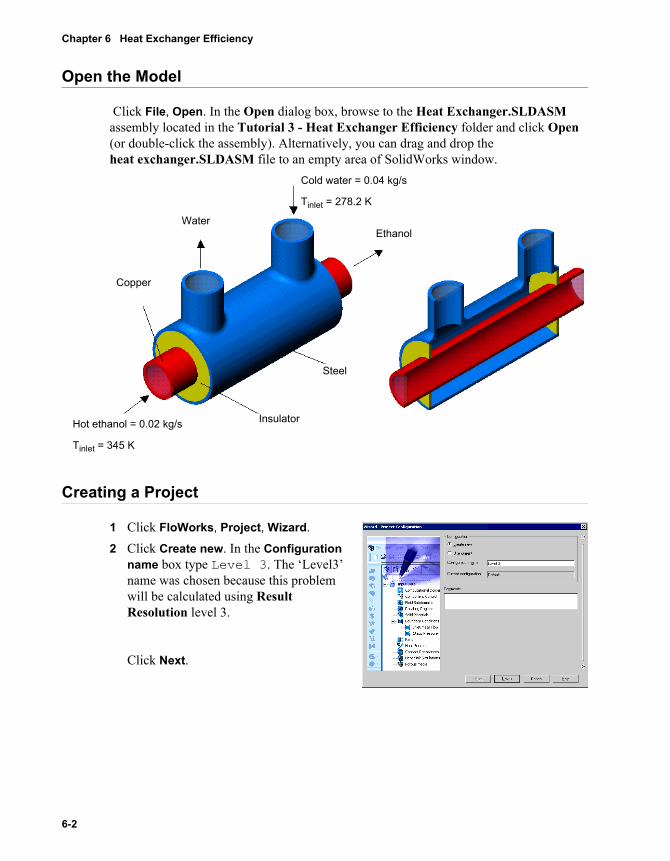
Click File, Open. In the Open dialog box, browse to the Heat Exchanger.SLDASM assembly located in the Tutorial 3 - Heat Exchanger Efficiency folder and click Open (or double-click the assembly). Alternatively, you can drag and drop the heat exchanger.SLDASM file to an empty area of SolidWorks window.

Creating a Project

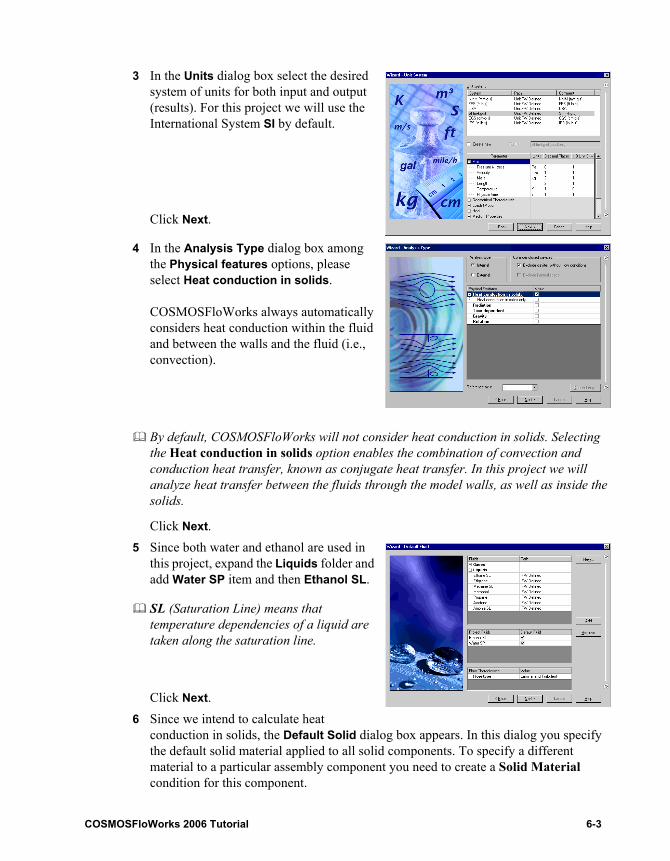
1 Click FloWorks, Project, Wizard. 2 Click Create new. In the Configuration

name box type Level 3. The ‘Level3’ name was chosen because this problem will be calculated using Result Resolution level 3.

Click Next.

Water

Cold water = 0.04 kg/s

Tinlet = 278.2 K

Copper

Ethanol

Steel

InsulatorHot ethanol = 0.02 kg/s

Tinlet = 345 K


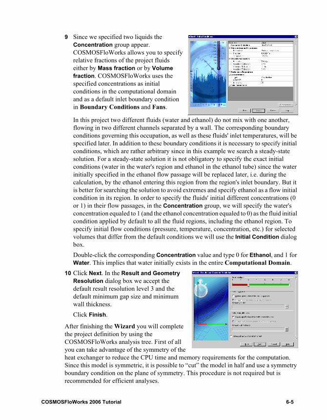
3 In the Units dialog box select the desired system of units for both input and output (results). For this project we will use the International System SI by default.

Click Next.

4 In the Analysis Type dialog box among the Physical features options, please select Heat conduction in solids.

COSMOSFloWorks always automatically considers heat conduction within the fluid and between the walls and the fluid (i.e., convection).

By default, COSMOSFloWorks will not consider heat conduction in solids. Selecting the Heat conduction in solids option enables the combination of convection and conduction heat transfer, known as conjugate heat transfer. In this project we will analyze heat transfer between the fluids through the model walls, as well as inside the solids.

Click Next.5 Since both water and ethanol are used in

this project, expand the Liquids folder and add Water SP item and then Ethanol SL.

SL (Saturation Line) means that temperature dependencies of a liquid are taken along the saturation line.

Click Next.6 Since we intend to calculate heat

conduction in solids, the Default Solid dialog box appears. In this dialog you specify the default solid material applied to all solid components. To specify a different material to a particular assembly component you need to create a Solid Material condition for this component.


6-4

If the material you wish to analyze is not under the Solids table you can click New and define a new substance in the Engineering Database. The heat exchanger in this project is constructed of steel, copper and insulators.

Click Steel,stainless to make it default material.Click Next.

If a component has been previously assigned a solid material by the SolidWorks’ Materials Editor, you can import this material into COSMOSFloWorks and apply it to the component by using the Insert Material from Model option accessible under Floworks, Tools.

7 In the Wall Condition dialog box, select Heat transfer coefficient as Default outer wall thermal condition.

This condition allows you to define the heat flux from the outer model walls to an external fluid (not modeled) by specifying the reference fluid temperature and the heat transfer coefficient value.

Set the Heat transfer coefficient value to 5 W/m2/K and the Temperature of external fluid to 263.2 K.In this project we also will not concern rough walls.Click Next.

8 In the Initial and Ambient Conditions dialog box specify initial values of the flow parameters. Since the inlet water temperature is equal to 278.2 K, we will specify it as an initial condition to be consistent with the specified boundary condition. Double-click the Value cell of the Temperature item and type 278.2.


9 Since we specified two liquids the Concentration group appear. COSMOSFloWorks allows you to specify relative fractions of the project fluids either by Mass fraction or by Volume fraction. COSMOSFloWorks uses the specified concentrations as initial conditions in the computational domain and as a default inlet boundary condition in Boundary Conditions and Fans.

In this project two different fluids (water and ethanol) do not mix with one another, flowing in two different channels separated by a wall. The corresponding boundary conditions governing this occupation, as well as these fluids' inlet temperatures, will be specified later. In addition to these boundary conditions it is necessary to specify initial conditions, which are rather arbitrary since in this example we search a steady-state solution. For a steady-state solution it is not obligatory to specify the exact initial conditions (water in the water's region and ethanol in the ethanol tube) since the water initially specified in the ethanol flow passage will be replaced later, i.e. during the calculation, by the ethanol entering this region from the region's inlet boundary. But it is better for searching the solution to avoid extremes and specify ethanol as a flow initial condition in its region. In order to specify the fluids' initial different concentrations (0 or 1) in their flow passages, in the Concentration group, we will specify the water's concentration equaled to 1 (and the ethanol concentration equaled to 0) as the fluid initial condition applied by default to all the fluid regions, including the ethanol region. To specify initial flow conditions (pressure, temperature, concentration, etc.) for selected volumes that differ from the default conditions we will use the Initial Condition dialog box.Double-click the corresponding Concentration value and type 0 for Ethanol, and 1 for Water. This implies that water initially exists in the entire Computational Domain.

10 Click Next. In the Result and Geometry Resolution dialog box we accept the default result resolution level 3 and the default minimum gap size and minimum wall thickness. Click Finish.

After finishing the Wizard you will complete the project definition by using the COSMOSFloWorks analysis tree. First of all you can take advantage of the symmetry of the heat exchanger to reduce the CPU time and memory requirements for the computation. Since this model is symmetric, it is possible to “cut” the model in half and use a symmetry boundary condition on the plane of symmetry. This procedure is not required but is recommended for efficient analyses.


6-6

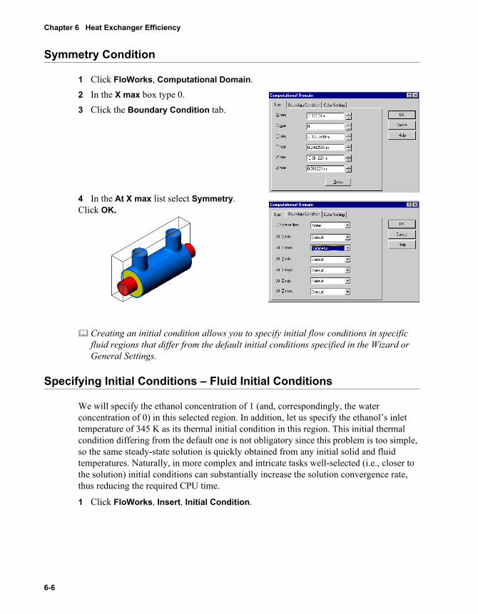
Symmetry Condition

1 Click FloWorks, Computational Domain.2 In the X max box type 0.3 Click the Boundary Condition tab.

4 In the At X max list select Symmetry.Click OK.

Creating an initial condition allows you to specify initial flow conditions in specific fluid regions that differ from the default initial conditions specified in the Wizard or General Settings.

Specifying Initial Conditions – Fluid Initial Conditions

We will specify the ethanol concentration of 1 (and, correspondingly, the water concentration of 0) in this selected region. In addition, let us specify the ethanol’s inlet temperature of 345 K as its thermal initial condition in this region. This initial thermal condition differing from the default one is not obligatory since this problem is too simple, so the same steady-state solution is quickly obtained from any initial solid and fluid temperatures. Naturally, in more complex and intricate tasks well-selected (i.e., closer to the solution) initial conditions can substantially increase the solution convergence rate, thus reducing the required CPU time.

1 Click FloWorks, Insert, Initial Condition.


To specify the initial condition within a fluid region we must specify this condition on the one of the faces lying on the region’s boundary - i.e. on the boundary between solid and fluid substances. The initial condition specified on the region’s boundary will be applied to the entire fluid region.

2 Select the Ethanol Inlet Lid inner face (in contact with the fluid).

If you want to specify an initial condition to a fluid region within a closed internal fluid volume, instead of creating this volume as a separate component (and disabling it), you can select any surface bounding this fluid volume to be automatically considered by the program as the volume to apply the fluid initial conditions.

3 Accept the default Coordinate system and the Reference axis. Click the Setting tab. On the Settings tab COSMOSFloWorks allows you to specify initial flow parameters, initial thermodynamic parameters, initial turbulence parameters (if the Show advanced parameters check box is selected), and initial concentrations.

These settings are applied to the fluid region inside the Tube component.

4 Double-click the Value cell of Temperature and type 345.

5 Expand the Substance Concentrations item and specify concentration as follows: Ethanol - 1, Water - 0.

6 Click OK. The new Initial Condition1 item appears in the analysis tree.7 To easily identify the specified condition you can

give a more descriptive name for the Initial Condition1 item. Right-click the Initial Condition1 item and select Properties. In the Name box type Hot Ethanol and click OK.

You can also click-pause-click an item to rename it directly in the COSMOSFloWorks analysis tree.


6-8

The specified initial condition means that initially hot (345 K) ethanol exists within the tube. Although the specification of this initial condition was optional it will result in a dramatic decrease in the total computation time. The next step is to specify boundary conditions to define the water and ethanol flows passing through the model.

Specifying Boundary Conditions

1 Right-click the Boundary Conditions icon and select Insert Boundary Condition. The Boundary Condition dialog box appears.

2 Select the Water Inlet Lid inner face (in contact with the fluid).The selected face appears in the Faces to apply boundary condition list.

3 Accept the default Inlet Mass Flow condition and the default Coordinate system and Reference axis. Click the Settings tab.

4 Double-click the Value cell of the Mass flow rate normal to face item and set it equal to 0.02 kg/s. Since the symmetry plane halves the opening we need to specify a half of the actual mass flow rate.

5 Expand the Thermodynamic Parameters item. The default temperature value is equal to the value specified as initial temperature in the Wizard. We accept this value.

6 Expand Substance Concentrations item to check that the concentration of the inlet fluid is the default concentration that you specified in the Wizard. The zero concentration for Ethanol implies that water is the only liquid entering the model through this opening.

7 Click OK. The new Inlet Mass Flow1 item appears in the analysis tree.

This boundary condition specifies that water enters the steel jacket at a mass flow rate of 0.04 kg/s and temperature of 278.2 K.


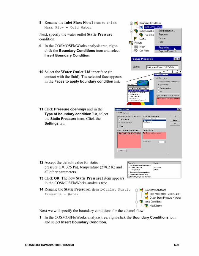
8 Rename the Inlet Mass Flow1 item to Inlet Mass Flow - Cold Water.

Next, specify the water outlet Static Pressure condition.

9 In the COSMOSFloWorks analysis tree, right-click the Boundary Conditions icon and select Insert Boundary Condition.

10 Select the Water Outlet Lid inner face (in contact with the fluid). The selected face appears in the Faces to apply boundary condition list.

11 Click Pressure openings and in the Type of boundary condition list, select the Static Pressure item. Click the Settings tab.

12 Accept the default value for static pressure (101325 Pa), temperature (278.2 K) and all other parameters.

13 Click OK. The new Static Pressure1 item appears in the COSMOSFloWorks analysis tree.

14 Rename the Static Pressure1 item to Outlet Static Pressure – Water.

Next we will specify the boundary conditions for the ethanol flow.

1 In the COSMOSFloWorks analysis tree, right-click the Boundary Conditions icon and select Insert Boundary Condition.


6-10

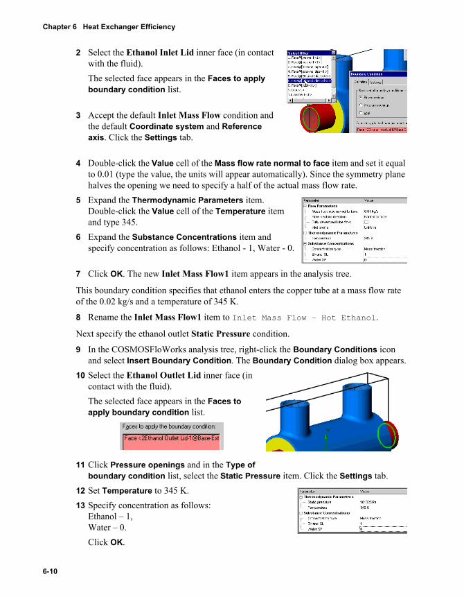
2 Select the Ethanol Inlet Lid inner face (in contact with the fluid).The selected face appears in the Faces to apply boundary condition list.

3 Accept the default Inlet Mass Flow condition and the default Coordinate system and Reference axis. Click the Settings tab.

4 Double-click the Value cell of the Mass flow rate normal to face item and set it equal to 0.01 (type the value, the units will appear automatically). Since the symmetry plane halves the opening we need to specify a half of the actual mass flow rate.

5 Expand the Thermodynamic Parameters item. Double-click the Value cell of the Temperature item and type 345.

6 Expand the Substance Concentrations item and specify concentration as follows: Ethanol - 1, Water - 0.

7 Click OK. The new Inlet Mass Flow1 item appears in the analysis tree.

This boundary condition specifies that ethanol enters the copper tube at a mass flow rate of the 0.02 kg/s and a temperature of 345 K.

8 Rename the Inlet Mass Flow1 item to Inlet Mass Flow – Hot Ethanol.

Next specify the ethanol outlet Static Pressure condition.

9 In the COSMOSFloWorks analysis tree, right-click the Boundary Conditions icon and select Insert Boundary Condition. The Boundary Condition dialog box appears.

10 Select the Ethanol Outlet Lid inner face (in contact with the fluid).The selected face appears in the Faces to apply boundary condition list.

11 Click Pressure openings and in the Type of boundary condition list, select the Static Pressure item. Click the Settings tab.

12 Set Temperature to 345 K.13 Specify concentration as follows:

Ethanol – 1,Water – 0. Click OK.


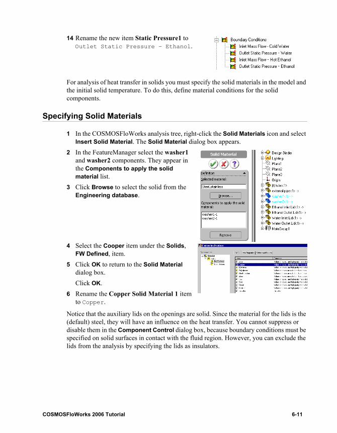
14 Rename the new item Static Pressure1 to Outlet Static Pressure – Ethanol.

For analysis of heat transfer in solids you must specify the solid materials in the model and the initial solid temperature. To do this, define material conditions for the solid components.

Specifying Solid Materials

1 In the COSMOSFloWorks analysis tree, right-click the Solid Materials icon and select Insert Solid Material. The Solid Material dialog box appears.

2 In the FeatureManager select the washer1 and washer2 components. They appear in the Components to apply the solid material list.

3 Click Browse to select the solid from the Engineering database.

4 Select the Cooper item under the Solids, FW Defined, item.

5 Click OK to return to the Solid Material dialog box.Click OK.

6 Rename the Copper Solid Material 1 item to Copper.

Notice that the auxiliary lids on the openings are solid. Since the material for the lids is the (default) steel, they will have an influence on the heat transfer. You cannot suppress or disable them in the Component Control dialog box, because boundary conditions must be specified on solid surfaces in contact with the fluid region. However, you can exclude the lids from the analysis by specifying the lids as insulators.


6-12

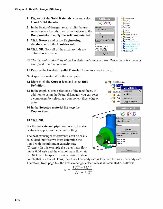
7 Right-click the Solid Materials icon and select Insert Solid Material.

8 In the FeatureManager, select all lid features. As you select the lids, their names appear in the Components to apply the solid material list.

9 Click Browse and in the Engineering database select the Insulator solid.

10 Click OK. Now all of the auxiliary lids are defined as insulators.

The thermal conductivity of the Insulator substance is zero. Hence there is no a heat transfer through an insulator.

11 Rename the Insulator Solid Material 1 item to Insulators.

Next specify a material for the inner pipe.

12 Right-click the Copper icon and select Edit Definition.

13 In the graphics area select one of the tube faces. In addition to using the FeatureManager, you can select a component by selecting a component face, edge or point.

14 In the Selected material list keep the Copper item.

15 Click OK.

For the last external pipe component, the steel is already applied as the default setting.

The heat exchanger effectiveness can be easily calculated, but first we must determine the liquid with the minimum capacity rate (C= ). In this example the water mass flow rate is 0.04 kg/s and the ethanol mass flow rate is 0.02 kg/s. The specific heat of water is about double that of ethanol. Thus, the ethanol capacity rate is less than the water capacity rate. Therefore, from page 6-2 the heat exchanger effectiveness is calculated as follows:

cm&

ε Thotinlet Thot

outlet–Thot

inlet TcoldInlet–

-------------------------------,=


where is the temperature of the ethanol at the inlet, is the temperature of the ethanol at the outlet, and is the temperature of the water at the inlet. Since we already know the ethanol temperature at the inlet (345 K) and the water temperature at the inlet (278.2 K), our goal is to determine the ethanol temperature at the outlet. The easiest and fastest way to find this parameter is to specify the corresponding engineering Goal.

Specifying a Surface Goal

1 In the COSMOSFloWorks analysis tree, right-click the Goals icon and select Insert Surface Goals.

2 In the COSMOSFloWorks analysis tree, select the Outlet Static Pressure - Ethanol item. The face that belongs to this boundary condition is automatically selected.

3 In the Parameter table select the Bulk Av. check box in the Temperature of Fluid row.

4 Accept selected Use for Conv check box to use this goal for convergence control.

5 In the Name template type SG Bulk Av T of Ethanol.

6 Click OK.

Click FloWorks, Project, Rebuild.

Adjusting Mesh Settings

1 Click FloWorks, Initial Mesh and switch off the automatic settings of initial mesh by clearing the Automatic settings check box.

2 On the Solid/Fluid Interface tab set the Curvature refinement level to 2 and the Curvature refinement criterion to 0.1 rad.

This will invoke additional cell refinement at the tube's interface, providing a more accurate heat exchange between the hot ethanol and the water.

3 Click OK.

Thotinlet - Thot

outlet -Tcold

inlet -


6-14

Running the Calculation

1 Click FloWorks, Solve, Run. The Run dialog box appears.2 Click Run.

After the calculation finishes you can obtain the temperature of interest by creating the corresponding Goal Plot.

Viewing the Goals

In additional to using the COSMOSFloWorks analysis tree you can use COSMOSFloWorks Toolbars to get fast and easy access to the most frequently used COSMOSFloWorks features. Toolbars are very convenient for displaying results.

Click View, Toolbars, COSMOSFloWorks Results, Main. The COSMOSFloWorks Results Main toolbar appears.

Click View, Toolbars, COSMOSFloWorks Results Insert. The COSMOSFloWorks Results Insert toolbar appears.

Click View, Toolbars, COSMOSFloWorks Results Display. The COSMOSFloWorks Results Display toolbar appears.

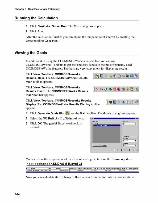
1 Click Generate Goals Plot on the Main toolbar. The Goals dialog box appears.2 Select the SG Bulk Av T of Ethanol item.3 Click OK. The goals1 Excel workbook is

created.

You can view the temperature of the ethanol leaving the tube on the Summary sheet.

Now you can calculate the exchanger effectiveness from the formula mentioned above:

heat exchanger.SLDASM [Level 3]Goal Name Unit Value Averaged Value Minimum Value Maximum Value Progress [%] Use In ConvergenceSG Bulk Average T of Ethanol [K] 339.9732883 339.994 339.962 340.108 100 Yes


Let us now look inside the exchanger to investigate the mechanisms for the heat transfer in the liquids and solids. First we will create a cut plot to see a temperature distribution.

Creating a Cut Plot

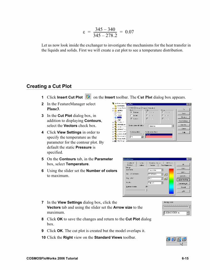
1 Click Insert Cut Plot on the Insert toolbar. The Cut Plot dialog box appears.2 In the FeatureManager select

Plane3.3 In the Cut Plot dialog box, in

addition to displaying Contours, select the Vectors check box.

4 Click View Settings in order to specify the temperature as the parameter for the contour plot. By default the static Pressure is specified.

5 On the Contours tab, in the Parameter box, select Temperature.

6 Using the slider set the Number of colors to maximum.

7 In the View Settings dialog box, click the Vectors tab and using the slider set the Arrow size to the maximum.

8 Click OK to save the changes and return to the Cut Plot dialog box.

9 Click OK. The cut plot is created but the model overlaps it.10 Click the Right view on the Standard Views toolbar.

ε 345 340–345 278.2–---------------------------- 0.07= =


6-16

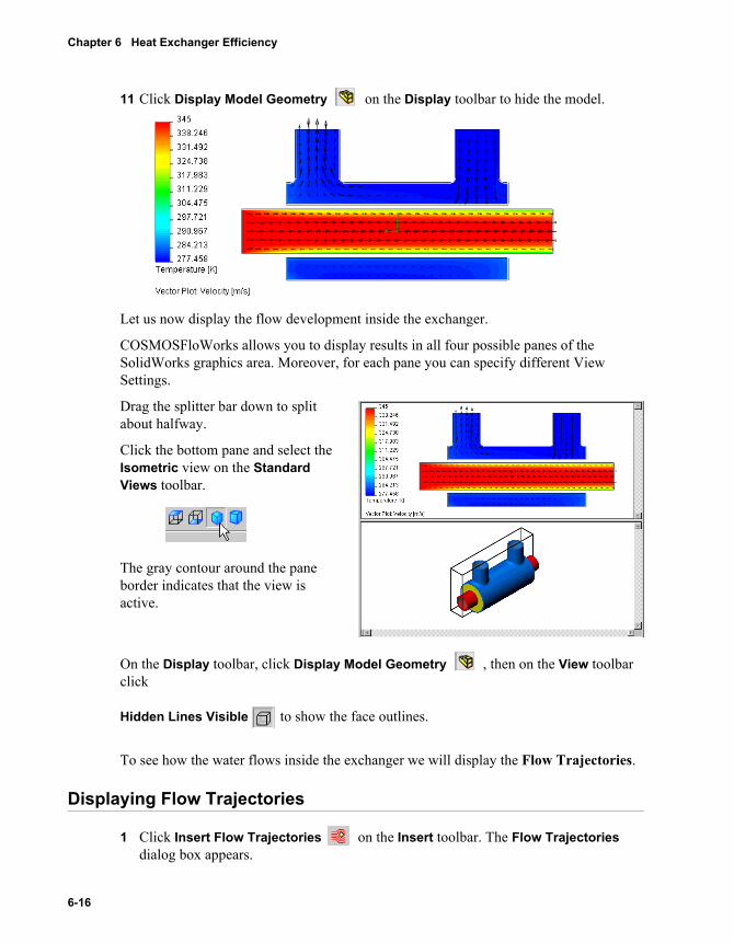
11 Click Display Model Geometry on the Display toolbar to hide the model.

Let us now display the flow development inside the exchanger.

COSMOSFloWorks allows you to display results in all four possible panes of the SolidWorks graphics area. Moreover, for each pane you can specify different View Settings.

Drag the splitter bar down to split about halfway.

Click the bottom pane and select the Isometric view on the Standard Views toolbar.

The gray contour around the pane border indicates that the view is active.

On the Display toolbar, click Display Model Geometry , then on the View toolbar click

Hidden Lines Visible to show the face outlines.

To see how the water flows inside the exchanger we will display the Flow Trajectories.

Displaying Flow Trajectories

1 Click Insert Flow Trajectories on the Insert toolbar. The Flow Trajectories dialog box appears.


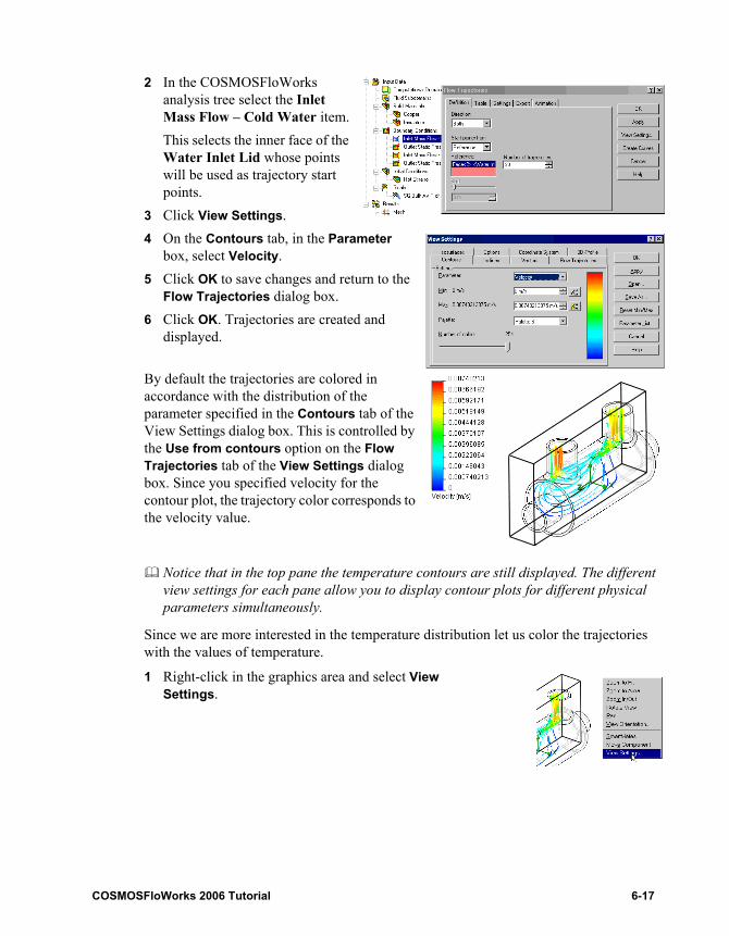
2 In the COSMOSFloWorks analysis tree select the Inlet Mass Flow – Cold Water item.This selects the inner face of the Water Inlet Lid whose points will be used as trajectory start points.

3 Click View Settings.4 On the Contours tab, in the Parameter

box, select Velocity.5 Click OK to save changes and return to the

Flow Trajectories dialog box.6 Click OK. Trajectories are created and

displayed.

By default the trajectories are colored in accordance with the distribution of the parameter specified in the Contours tab of the View Settings dialog box. This is controlled by the Use from contours option on the Flow Trajectories tab of the View Settings dialog box. Since you specified velocity for the contour plot, the trajectory color corresponds to the velocity value.

Notice that in the top pane the temperature contours are still displayed. The different view settings for each pane allow you to display contour plots for different physical parameters simultaneously.

Since we are more interested in the temperature distribution let us color the trajectories with the values of temperature.

1 Right-click in the graphics area and select View Settings.


6-18

2 On the Contours tab, in the Parameter box, select Temperature.

3 Click OK. Immediately the trajectories are updated.

The water temperature range is less than the default overall (Global) range (277 – 345),so all of the trajectories are the same blue color. To get more information about the temperature distribution in water you can manually specify the range of interest.

Let us display temperatures in the range of inlet-outlet water temperature.

The water minimum temperature value is near 277 K. The maximum water temperature value can be determined by using the Surface Parameters command at the water outlet.

Surface Parameters allows you to display parameter values (minimum, maximum, average and integral) calculated over the specified surface. All parameters are divided into two categories: Local and Integral. For local parameters (pressure, temperature, velocity etc.) the maximum, minimum and average values are evaluated.

Computation of Surface Parameters

1 Click Computation of Surface Parameters on the Insert toolbar. The Surface Parameters dialog box appears.

2 Click the Outlet Static pressure - Water item to select the face of the water outlet lid.

3 Click Evaluate.4 After the parameters are calculated

click the Local tab.

You can see that the average water temperature at the outlet is about 280 K. This value will be used as the maximum value.


5 Click Cancel to close the dialog.

Now you can specify the display range for the temperature.

Specifying the Parameter Display Range

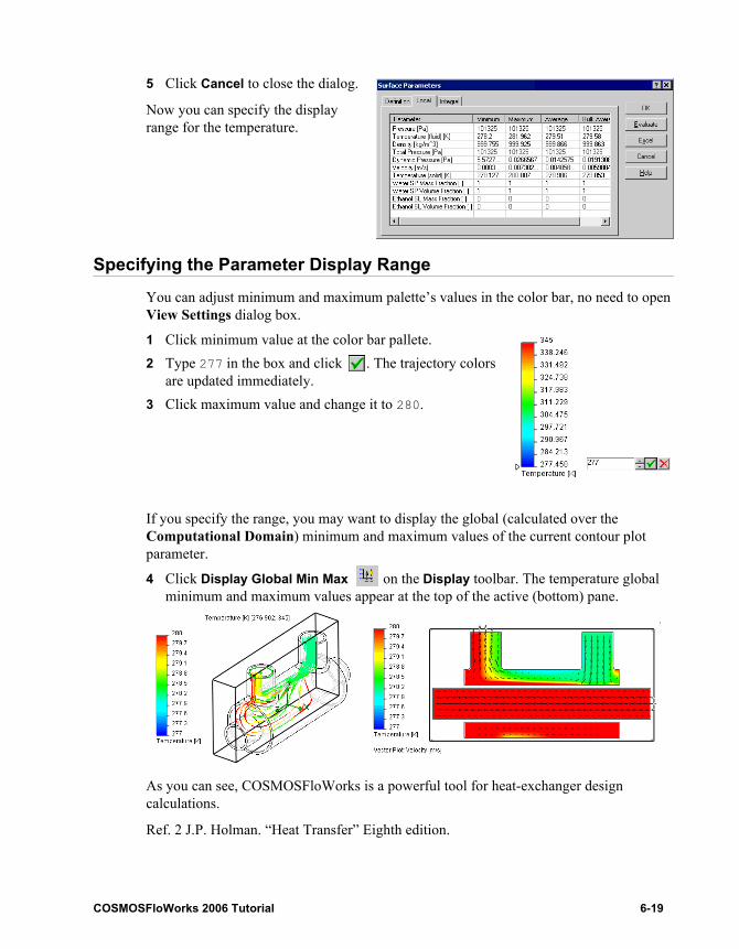
You can adjust minimum and maximum palette’s values in the color bar, no need to open View Settings dialog box.

1 Click minimum value at the color bar pallete. 2 Type 277 in the box and click . The trajectory colors

are updated immediately.3 Click maximum value and change it to 280.

If you specify the range, you may want to display the global (calculated over the Computational Domain) minimum and maximum values of the current contour plot parameter.

4 Click Display Global Min Max on the Display toolbar. The temperature global minimum and maximum values appear at the top of the active (bottom) pane.

As you can see, COSMOSFloWorks is a powerful tool for heat-exchanger design calculations.

Ref. 2 J.P. Holman. “Heat Transfer” Eighth edition.


6-20

heat exchanger efficiency - rice university · pdf filecosmosfloworks 2006 tutorial 6-1 6 heat...

Documents