heat 4e sm chap05
TRANSCRIPT
PROPRIETARY MATERIAL. © 2011 The McGraw-Hill Companies, Inc. Limited distribution permitted only to teachers and educators for course preparation. If you are a student using this Manual, you are using it without permission.
5-1
Solutions Manual for
Heat and Mass Transfer: Fundamentals & Applications Fourth Edition
Yunus A. Cengel & Afshin J. Ghajar McGraw-Hill, 2011
Chapter 5 NUMERICAL METHODS IN HEAT
CONDUCTION
PROPRIETARY AND CONFIDENTIAL This Manual is the proprietary property of The McGraw-Hill Companies, Inc. (“McGraw-Hill”) and protected by copyright and other state and federal laws. By opening and using this Manual the user agrees to the following restrictions, and if the recipient does not agree to these restrictions, the Manual should be promptly returned unopened to McGraw-Hill: This Manual is being provided only to authorized professors and instructors for use in preparing for the classes using the affiliated textbook. No other use or distribution of this Manual is permitted. This Manual may not be sold and may not be distributed to or used by any student or other third party. No part of this Manual may be reproduced, displayed or distributed in any form or by any means, electronic or otherwise, without the prior written permission of McGraw-Hill.
PROPRIETARY MATERIAL. © 2011 The McGraw-Hill Companies, Inc. Limited distribution permitted only to teachers and educators for course preparation. If you are a student using this Manual, you are using it without permission.
5-2
Why Numerical Methods?
5-1C Analytical solutions provide insight to the problems, and allows us to observe the degree of dependence of solutions on certain parameters. They also enable us to obtain quick solution, and to verify numerical codes. Therefore, analytical solutions are not likely to disappear from engineering curricula.
5-2C Analytical solution methods are limited to highly simplified problems in simple geometries. The geometry must be such that its entire surface can be described mathematically in a coordinate system by setting the variables equal to constants. Also, heat transfer problems can not be solved analytically if the thermal conditions are not sufficiently simple. For example, the consideration of the variation of thermal conductivity with temperature, the variation of the heat transfer coefficient over the surface, or the radiation heat transfer on the surfaces can make it impossible to obtain an analytical solution. Therefore, analytical solutions are limited to problems that are simple or can be simplified with reasonable approximations.
5-3C In practice, we are most likely to use a software package to solve heat transfer problems even when analytical solutions are available since we can do parametric studies very easily and present the results graphically by the press of a button. Besides, once a person is used to solving problems numerically, it is very difficult to go back to solving differential equations by hand.
5-4C The energy balance method is based on subdividing the medium into a sufficient number of volume elements, and then applying an energy balance on each element. The formal finite difference method is based on replacing derivatives by their finite difference approximations. For a specified nodal network, these two methods will result in the same set of equations.
5-5C The analytical solutions are based on (1) driving the governing differential equation by performing an energy balance on a differential volume element, (2) expressing the boundary conditions in the proper mathematical form, and (3) solving the differential equation and applying the boundary conditions to determine the integration constants. The numerical solution methods are based on replacing the differential equations by algebraic equations. In the case of the popular finite difference method, this is done by replacing the derivatives by differences. The analytical methods are simple and they provide solution functions applicable to the entire medium, but they are limited to simple problems in simple geometries. The numerical methods are usually more involved and the solutions are obtained at a number of points, but they are applicable to any geometry subjected to any kind of thermal conditions.
5-6C The experiments will most likely prove engineer B right since an approximate solution of a more realistic model is more accurate than the exact solution of a crude model of an actual problem.
PROPRIETARY MATERIAL. © 2011 The McGraw-Hill Companies, Inc. Limited distribution permitted only to teachers and educators for course preparation. If you are a student using this Manual, you are using it without permission.
5-3
Finite Difference Formulation of Differential Equations
5-7C A point at which the finite difference formulation of a problem is obtained is called a node, and all the nodes for a problem constitute the nodal network. The region about a node whose properties are represented by the property values at the nodal point is called the volume element. The distance between two consecutive nodes is called the nodal spacing, and a differential equation whose derivatives are replaced by differences is called a difference equation.
5-8 The finite difference formulation of steady two-dimensional heat conduction in a medium with heat generation and constant thermal conductivity is given by
022 ,
22 ∆1,,1,,1,,1 =+
+−+
+− +−+ eTTTTTT nmnmnmnmnmnmn &
ase by simply adding another index j to the temperature in the z direction, and another difference term for the z direction as
−m
∆ kyx
in rectangular coordinates. This relation can be modified for the three-dimensional c
0222 ,,
21,,,,1,,
2,1,,,,1,
2,,1,,,,1 =+
∆
+−+
∆
+−+
∆
+− +−+−+−
ke
z
TTT
y
TTT
x
TTT jnmjnmjnmjnmjnmjnmjnmjnmjnmjnm &
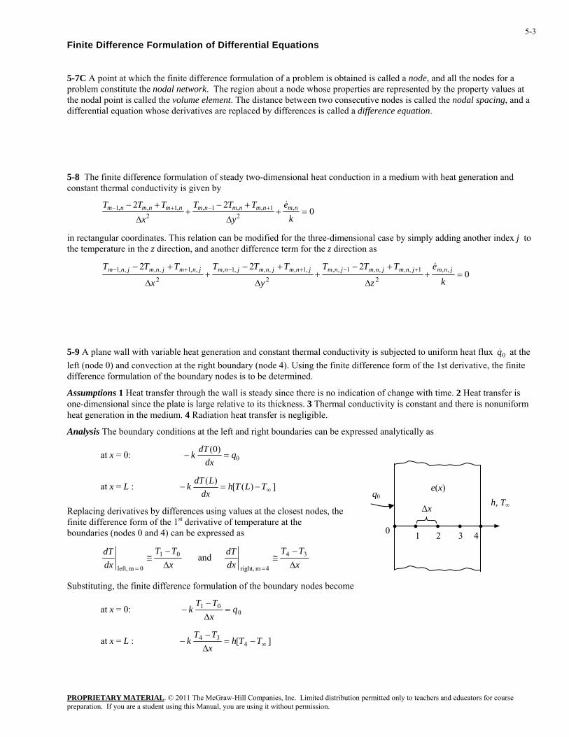
5-9 A plane wall with variable heat generation and constant thermal conductivity is subjected to uniform heat flux 0q& at theleft (node 0) and convection at the right boundary (node 4). Using th
e finite difference form of the 1st derivative, the finite
mal conductivity is constant and there is nonuniform
Analysis ft and right boundaries can be expressed analytically as
at x = 0:
difference formulation of the boundary nodes is to be determined.
Assumptions 1 Heat transfer through the wall is steady since there is no indication of change with time. 2 Heat transfer is one-dimensional since the plate is large relative to its thickness. 3 Therheat generation in the medium. 4 Radiation heat transfer is negligible.
The boundary conditions at the le
0)0( q
dxdTk =−
q0
∆x
e(x)
1
h, T∞
• •• ••0 2 3 4
at x = L : ])([)(
∞−=− TLThdx
LdTk
Replacing derivatives by differences using values at the closest nodes, the of the 1st derivative of temperature at the
ndaries (nodes 0 and 4) can be expressed as finite difference formbou
xTT
dxdT
xTT
dxdT
∆−
≅∆−
≅ 3401 and =4 m right,
Substituting, the finite difference formulation of the boundary nodes become
at x = 0:
= 0 m left,
001 q
xTT
k =∆−
−
at x = L : ][ 434
∞−=∆−
− TThxTT
k
PROPRIETARY MATERIAL. © 2011 The McGraw-Hill Companies, Inc. Limited distribution permitted only to teachers and educators for course preparation. If you are a student using this Manual, you are using it without permission.
5-4
e
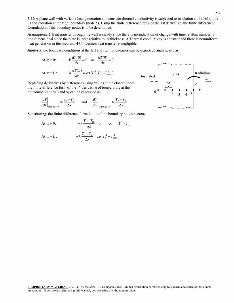
ime. 2 Heat transfer is e-dimen e plate is large relative to its thickness. 3 Thermal conductivity is constant and there is nonuniform t gen di m. 4 Convection heat transfer is negligible.
alysis nditions at the left and right boundaries can be expressed analytically as
5-10 A plane wall with variable heat generation and constant thermal conductivity is subjected to insulation at the left (nod0) and radiation at the right boundary (node 5). Using the finite difference form of the 1st derivative, the finite difference formulation of the boundary nodes is to be determined.
Assumptions 1 Heat transfer through the wall is steady since there is no indication of change with ton sional since thhea eration in the me u
An The boundary co
At x = 0: 0or 0 ==−dxdx
k
At x = L :
)0()0( dTdT
])([)( 4 LT
LdTk =− εσ 4
surrTdx
−
boundari
Replacing derivatives by differences using values at the closest nodes, the finite difference form of the 1st derivative of temperature at the
es (nodes 0 and 5) can be expressed as
xTT
dxdT
xdx ∆= 0 m left,
TTdT∆−
≅−
≅=
45
5 m right,
01 and
Substituting, the finite difference formulation of the boundary nodes become
At x = 0:
Insulated
∆x
(x)
1
ε
•
e
• • ••0 2 3 4•
5
Tsurr
adiation R
0101 or 0 TT
xTT
k ==∆−
−
][ 445
45surrTT
xTT
k −=∆−
− εσ At x = L :
PROPRIETARY MATERIAL. © 2011 The McGraw-Hill Companies, Inc. Limited distribution permitted only to teachers and educators for course preparation. If you are a student using this Manual, you are using it without permission.
5-5
One-Dimensional Steady Heat Conduction
5-11C The finite difference form of a heat conduction problem by the energy balance method is obtained by subdividing the medium into a sufficient number of volume elements, and then applying an energy balance on each element. This is done by first selecting the nodal points (or nodes) at which the temperatures are to be determined, and then forming elements (or control volumes) over the nodes by drawing lines through the midpoints between the nodes. The properties at the node such as the temperature and the rate of heat generation represent the average properties of the element. The temperature is assumed to vary linearly between the nodes, especially when expressing heat conduction between the elements using Fourier’s law.
5-12C The basic steps involved in the iterative Gauss-Seidel method are: (1) Writing the equations explicitly for each unknown (the unknown on the left-hand side and all other terms on the right-hand side of the equation), (2) making a reasonable initial guess for each unknown, (3) calculating new values for each unknown, always using the most recent values, and (4) repeating the process until desired convergence is achieved.
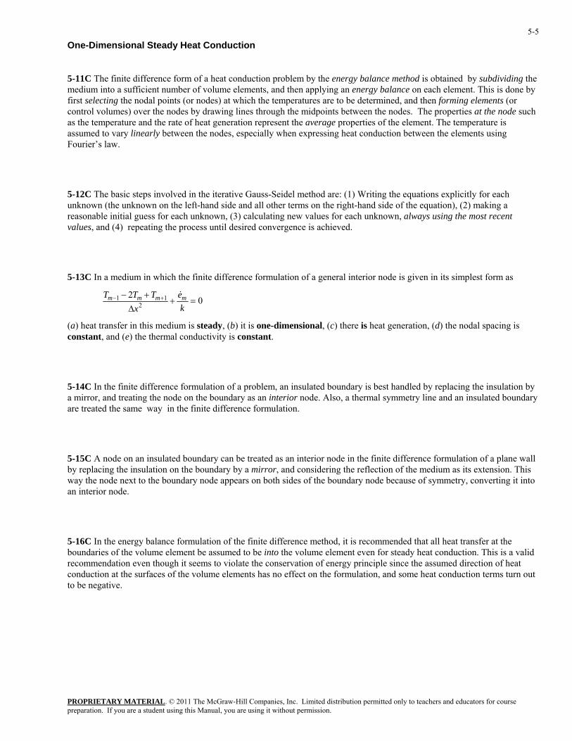
5-13C In a medium in which the finite difference formulation of a general interior node is given in its simplest form as
022
11 =+∆
+− +−
ke
xTTT mmmm &
(a) heat transfer in this medium is steady, (b) it is one-dimensional, (c) there is heat generation, (d) the nodal spacing is constant, and (e) the thermal conductivity is constant.
5-14C In the finite difference formulation of a problem, an insulated boundary is best handled by replacing the insulation by a mirror, and treating the node on the boundary as an interior node. Also, a thermal symmetry line and an insulated boundary are treated the same way in the finite difference formulation.
5-15C A node on an insulated boundary can be treated as an interior node in the finite difference formulation of a plane wall by replacing the insulation on the boundary by a mirror, and considering the reflection of the medium as its extension. This way the node next to the boundary node appears on both sides of the boundary node because of symmetry, converting it into an interior node.
5-16C In the energy balance formulation of the finite difference method, it is recommended that all heat transfer at the boundaries of the volume element be assumed to be into the volume element even for steady heat conduction. This is a valid recommendation even though it seems to violate the conservation of energy principle since the assumed direction of heat conduction at the surfaces of the volume elements has no effect on the formulation, and some heat conduction terms turn out to be negative.
PROPRIETARY MATERIAL. © 2011 The McGraw-Hill Companies, Inc. Limited distribution permitted only to teachers and educators for course preparation. If you are a student using this Manual, you are using it without permission.
5-6
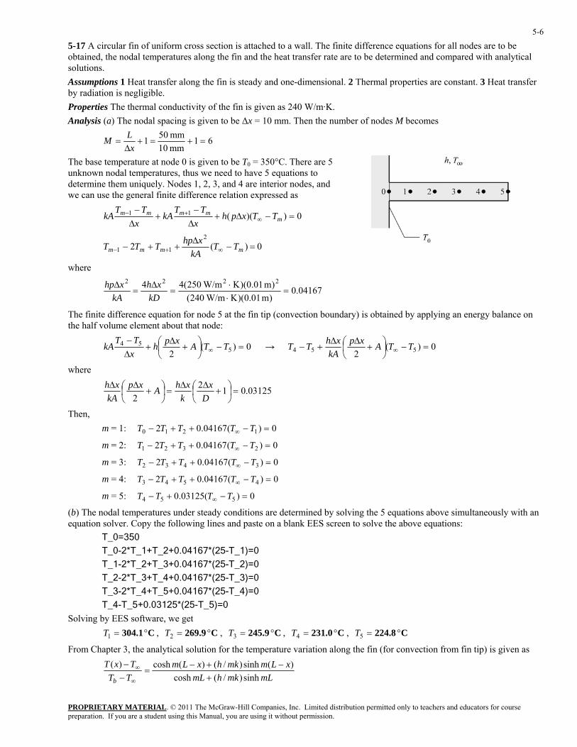
5-17 A circular fin of uniform cross section is attached to a wall. The finite difference equations for all nodes are to be obtained, the nodal temperatures along the fin and the heat transfer rate are to be determined and compared with analytical solutions. Assumptions 1 Heat transfer along the fin is steady and one-dimensional. 2 Thermal properties are constant. 3 Heat transfer by radiation is negligible. Properties The thermal conductivity of the fin is given as 240 W/m·K. Analysis (a) The nodal spacing is given to be ∆x = 10 mm. Then the number of nodes M becomes
61mm 10∆mm 501 =+=+=
xLM
5
es, and we can use the general finite difference relation expressed as
The base temperature at node 0 is given to be T0 = 350°C. There areunknown nodal temperatures, thus we need to have 5 equations to determine them uniquely. Nodes 1, 2, 3, and 4 are interior nod
0))((11 =−∆+∆−
+∆−
∞+−
mmmmm TTxph
xTT
kAx
TTkA
0)(22
11 =−∆
++− ∞+− mmmm TTkA
xhpTTT
where
04167.0 W/m240(
)m 01.0)(K W/m250(44 2222=
⋅=
∆=
∆kD
xhkA
xhp )m 01.0)(K⋅
he finite d equation for node 5 at the fin tip (convection boundary) is obtained by applying an energy balance on ent about that node:
T ifferencethe half volume elem
0)(2 5
54 =−⎟⎠⎞
⎜⎝⎛ +
∆+
∆−
∞ TTAxphxTT
kA → 0)(2 554 =−⎟
⎠⎞
⎜⎝⎛ +
∆∆+− ∞ TTAxp
kAxhTT
where
03125.0122
=⎟⎠⎞
⎜⎝⎛ +
∆∆=⎟
⎠⎞
⎜⎛∆ pxh ⎝
+∆
Dx
kxhAx
kA
Then, m = 1: 0)(04167.02 1210 =−++− ∞ TTTTT
m = 2: 0)(04167.02 2321 =−++ ∞ TTTTT −
m = 3: 0)(04167.02 3432 =−++− TTTTT ∞
m = 4: 0)(04167.02 4543 =−++− ∞ TTTTT
m = 5: 054 +−TT 0)(03125. 5 =−∞ TT
rmined by solving the 5 equations above simultaneously with an nk EES screen to solve the above equations:
67*(25-T_3)=0
T 2*T_4+T_5+ 7*(25-T_4)=
Solving by EES software, we get , ,
(b) The nodal temperatures under steady conditions are deteequation solver. Copy the following lines and paste on a bla T_0=350
T_0-2*T_1+T_2+0.04167*(25-T_1)=0
T_1-2*T_2+T_3+0.04167*(25-T_2)=0
T_2-2*T_3+T_4+0.041
_3- 0.0416 0
T_4-T_5+0.03125*(25-T_5)=0
C 304.1 °=1T C 269.9 °=2T C 245.9 °=3T , C 231.0 °= C 224.8 °=5T 4T ,
From Chapter 3, the analytical solution for the temperature variation along the fin (for convection from fin tip) is given as
mLmkhmL
xLmmkhxLmTTTxT
b sinh)/(cosh)(sinh)/()(cosh)(
+−+−
=−−
∞
∞
PROPRIETARY MATERIAL. © 2011 The McGraw-Hill Companies, Inc. Limited distribution permitted only to teachers and educators for course preparation. If you are a student using this Manual, you are using it without permission.
5-7
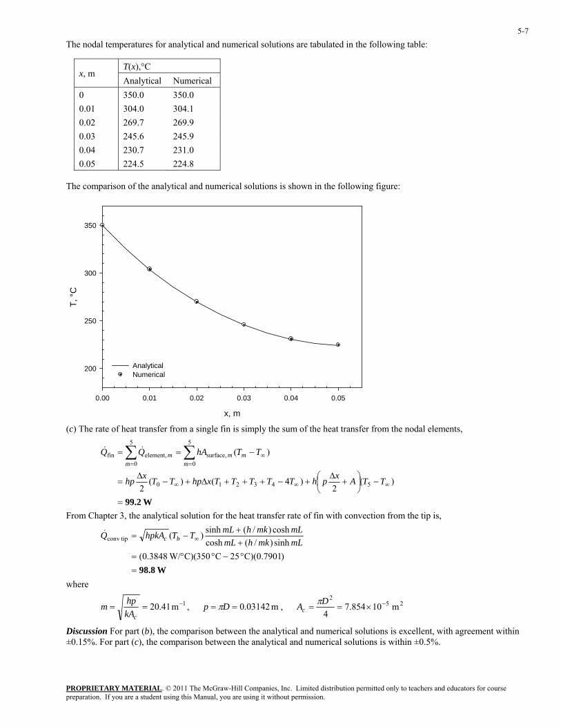
The nodal temperatures for analytical and numerical solutions are tabulated in the following table:
T(x),°C x, m
Analytical Numerical 0 350.0 350.0 0.01 304.0 304.1 0.02 269.7 269.9 0.03 245.6 245.9 0.04 230.7 231.0 0.05 224.5 224.8
The comparison of the analytical and numerical solutions is shown in the following figure:
x, m
0.00 0.01 0.02 0.03 0.04 0.05
200
250
300
350
Analytical
T, °
C
Numerical
(c) The rate of heat transfer from a single fin is simply the sum of the heat transfer from the nodal elements,
W99.2=
−⎟⎠⎞
⎜⎝⎛ +
∆+−+++∆+−
∆=
−==
∞∞∞
=∞
=∑∑
)(2
)4()(2
)(
543210
5
0 surface,
5
0 element,fin
TTAxphTTTTTxhpTTxhp
TThAQQm
mmm
m&&
From Chapter 3, the analytical solution for the heat transfer rate of fin with convection from the tip is,
W98.8=
°−°°=++
−= ∞
)7901.0)(C 25C 350)(C W/3848.0(sinh)/(coshcosh)/(sinh)( tipconv mLmkhmL
mLmkhmLTThpkAQ bc&
where
1m 41.20 −==ckA
hpm , m 03142.0== Dp π , 252
m 10854.74
−×==DAcπ
Discussion For part (b), the comparison between the analytical and numerical solutions is excellent, with agreement within ±0.15%. For part (c), the comparison between the analytical and numerical solutions is within ±0.5%.
PROPRIETARY MATERIAL. © 2011 The McGraw-Hill Companies, Inc. Limited distribution permitted only to teachers and educators for course preparation. If you are a student using this Manual, you are using it without permission.
5-8
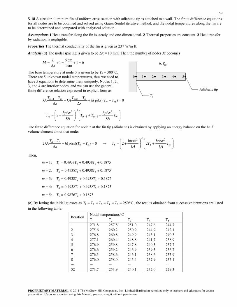
5-18 A circular aluminum fin of uniform cross section with adiabatic tip is attached to a wall. The finite difference equations for all nodes are to be obtained and solved using Gauss-Seidel iterative method, and the nodal temperatures along the fin are to be determined and compared with analytical solution.
Assumptions 1 Heat transfer along the fin is steady and one-dimensional. 2 Thermal properties are constant. 3 Heat transfer by radiation is negligible.
Properties The thermal conductivity of the fin is given as 237 W/m·K.
Analysis (a) The nodal spacing is given to be ∆x = 10 mm. Then the number of nodes M becomes
61cm 1∆cm 51 =+=+=
xLM
2,
finite difference relation expressed in explicit form as
The base temperature at node 0 is given to be T0 = 300°C. There are 5 unknown nodal temperatures, thus we need to have 5 equations to determine them uniquely. Nodes 1, 3, and 4 are interior nodes, and we can use the general
0))((11 =−∆+∆−
+∆−
∞+−
mmmmm TTxph
xTT
kAx
TTkA
⎟⎟ ⎠⎝⎠⎝
The finite difference equation for
⎞⎜⎜⎛ ∆
++⎟⎟⎞
⎜⎜⎛ ∆
+= ∞+−
−
TkA
xhpTTkA
xhpT mmm
2
11
122
node 5 at the fin tip (adiabatic) is obtained by applying an energy balance on the half volume element about that node:
0))((2 554 − =−∆+
∆ ∞ TTxphxTT
kA → ⎟⎟⎠
⎞⎜⎜⎝
⎛ ∆+⎟
⎟⎠
⎞⎜⎜⎝
⎛ ∆+= ∞
−
TkA
xhpTkA
xhpT2
4
12
5 22
Then,
m = 1: 1875.04938.04938.0 201 ++= TTT
m = 2: 1875.04938.04938.0 312 ++= TTT
m = 3: 1875.04938.04938.0 423 ++= TTT
m = 4: 4 1875.04938.04938.0 53 ++= TTT
guesses as , the results obtained from successive iterations are listed in the following table:
dal temp ture,°C
m = 5: 09876.0 45 += TT
(b) By letting the initial
1875.
C 25054321 °===== TTTTT
No eraIteration T1 T2 T3 T4 T5
1 271.8 257.8 251.0 247.6 244.7 2 275.6 260.2 250.9 244.9 242.1 3 276.8 260.8 249.9 243.1 240.3 4 277.1 260.4 248.8 241.7 238.9 5 276.9 259.8 247.8 240.5 237.7 6 276.6 259.2 246.9 239.5 236.7 7 276.3 258.6 246.1 238.6 235.9 8 276.0 .0 .4 .9 .1 258 245 237 235··· ··· ··· ··· ··· ··· 52 273.7 253.9 240.1 232.0 229.3
PROPRIETARY MATERIAL. © 2011 The McGraw-Hill Companies, Inc. Limited distribution permitted only to teachers and educators for course preparation. If you are a student using this Manual, you are using it without permission.
5-9
1T , 2T , 240.1
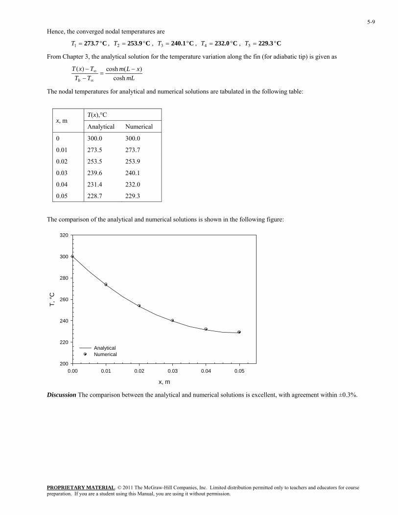
Hence, the converged nodal temperatures are
= = °C 273.7 ° C 253.9 ° C C 232.0 °=4T , C 229.3 °=5T =3T ,
From Chapter 3, the analytical solution for the temperature variation along the fin (for adiabatic tip) is given as
mL
xLmTTTxT
b cosh)(cosh)( −
=−−
∞
∞
The nodal temperatures for analytical and numerical solutions are tabulated in the following table:
T(x),°C x, m
Analytical Numerical
0 300.0 300.0
0.01 273.5 273.7
0.02 253.5 253.9
0.03 239.6 240.1
0.04 231.4 232.0
0.05 228.7 229.3
The comparison of the analytical and numerical solutions is shown in the following figure:
x, m
0.00 0.01 0.02 0.03 0.04 0.05
T, °
C
200
220
240
260
280
300
320
AnalyticalNumerical
Discussion The comparison between the analytical and numerical solutions is excellent, with agreement within ±0.3%.
PROPRIETARY MATERIAL. © 2011 The McGraw-Hill Companies, Inc. Limited distribution permitted only to teachers and educators for course preparation. If you are a student using this Manual, you are using it without permission.
5-10
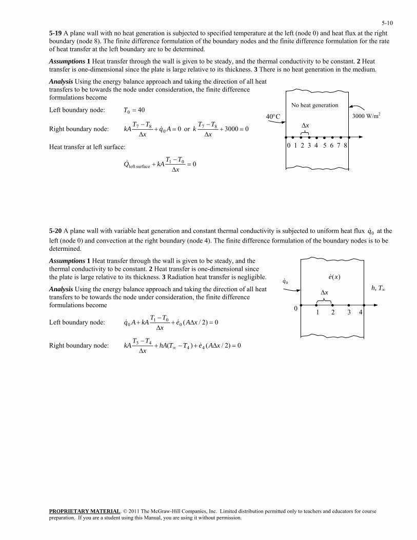
5-19 A plane wall with no heat generation is subjected to specified temperature at the left (node 0) and heat flux at the right boundary (node 8). The finite difference formulation of the boundary nodes and the finite difference formulation for the rate of heat transfer at the left boundary are to be determined.
Assumptions 1 Heat transfer through the wall is given to be steady, and the thermal conductivity to be constant. 2 Heat transfer is one-dimensional since the plate is large relative to its thickness. 3 There is no heat generation in the medium.
Analysis Using the energy balance approach and taking the direction of all heat transfers to be towards the node under consideration, the finite difference formulations become
40°C∆x
No heat generation
•
3000 W/m2
• • •• •• ••0 1 2 3 4 5 6 7 8
Left boundary node: 400 =T
Right boundary node: 03000or 0 870
87 =+∆−
=+∆−
xTT
kAqxTT
kA &
Heat transfer at left surface:
001surfaceleft =
∆−
+xTT
kAQ&
5-20 A plane wall with variable heat generation and constant thermal conductivity is subjected to uniform heat flux 0q& at theleft (node 0) an
d convection at the right boundary (node 4). The finite difference formulation of the boundary nodes is to be
heat the node under consideration, the finite difference
formulations become
Left boundary node:
determined.
Assumptions 1 Heat transfer through the wall is given to be steady, and the thermal conductivity to be constant. 2 Heat transfer is one-dimensional since
∆x
)(xe&
1
h, T∞
•
0q&
•• ••0 2 3 4
the plate is large relative to its thickness. 3 Radiation heat transfer is negligible.
Analysis Using the energy balance approach and taking the direction of alltransfers to be towards
0)2/(001
0 =∆+∆−
+ xAexTT
kAAq &&
0)2/()( 4443 =∆+−+
∆−
∞ xAeTThAxTT
kA & Right boundary node:
PROPRIETARY MATERIAL. © 2011 The McGraw-Hill Companies, Inc. Limited distribution permitted only to teachers and educators for course preparation. If you are a student using this Manual, you are using it without permission.
5-11
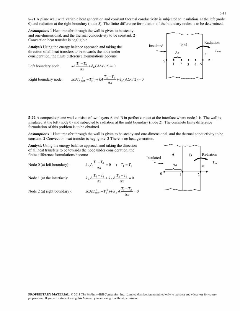
5-21 A plane wall with variable heat generation and constant thermal conductivity is subjected to insulation at the left (node 0) and radiation at the right boundary (node 5). The finite difference formulation of the boundary nodes is to be determined.
Assumptions 1 Heat transfer through the wall is given to be steady and one-dimensional, and the thermal conductivity to be constant. 2 Convection heat transfer is negligible.
Analysis Using the energy balance approach and taking the direction of all heat transfers to be towards the node under consideration, the finite difference formulations become
Left boundary node: 0)2/(001 =∆+
∆−
xAexTT
kA &
Right boundary node: 0)2/()( 5544
54
surr =∆+∆−
+− xAexTT
kATTAσ &ε
ll is diation at the right boundary (node 2). The complete finite difference
nsional, and the thermal conductivity to be eneration.
ode under consideration, the
finite difference formulations become
Node 0 (at left boundary):
Insulated
∆x
1
ε•
)(xe& Radiation
Tsurr
54•0 • ••
3•2
5-22 A composite plane wall consists of two layers A and B in perfect contact at the interface where node 1 is. The wainsulated at the left (node 0) and subjected to raformulation of this problem is to be obtained.
Assumptions 1 Heat transfer through the wall is given to be steady and one-dimeconstant. 2 Convection heat transfer is negligible. 3 There is no heat g
Analysis Using the energy balance approach and taking the directionof all heat transfers to be towards the n
Insulated
∆x
1
ε
• ••0 2
A
Tsurr
RadiationB
0101 0 TT
xTT
Ak A =→=∆−
01210 =∆−
+∆−
xTT
AkxTT
Ak BA Node 1 (at the interface):
0)( 2142
4surr =
∆−
+−xTT
AkTTA Bεσ Node 2 (at right boundary):
PROPRIETARY MATERIAL. © 2011 The McGraw-Hill Companies, Inc. Limited distribution permitted only to teachers and educators for course preparation. If you are a student using this Manual, you are using it without permission.
5-12
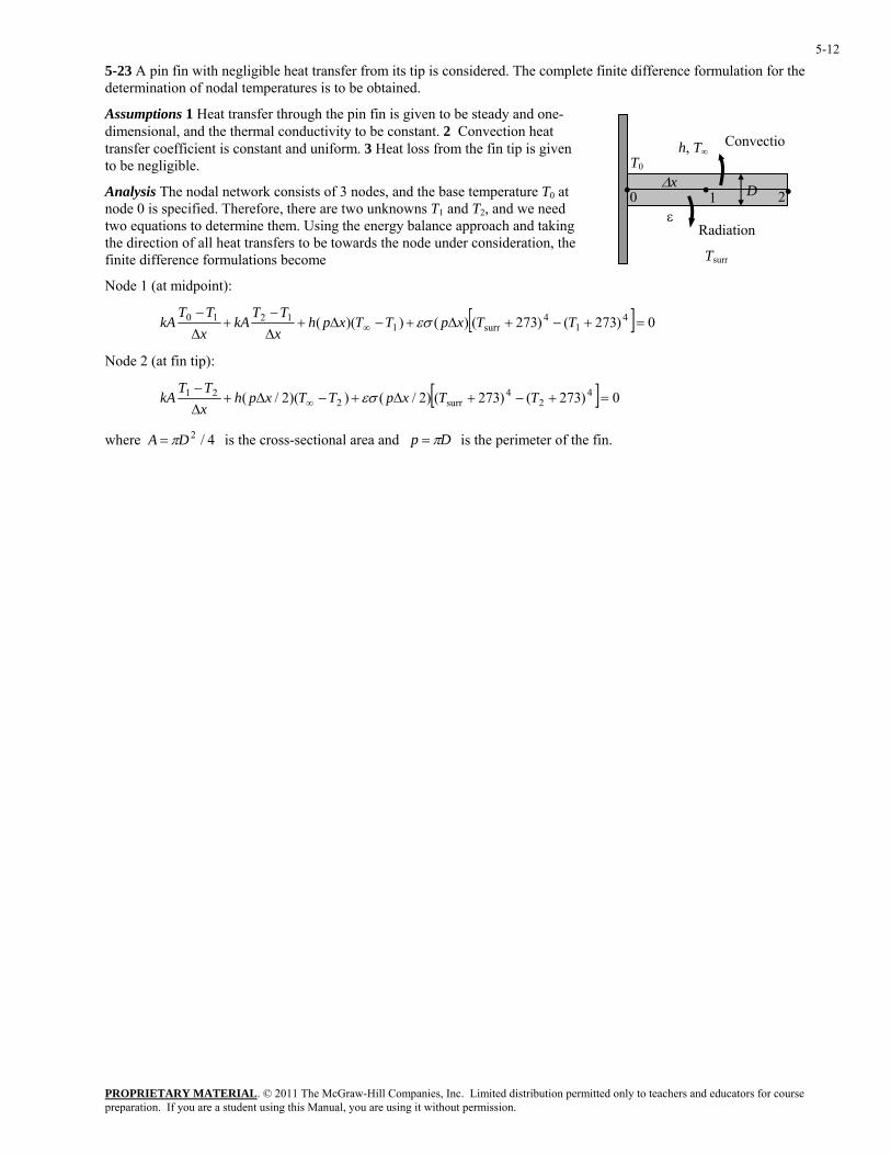
5-23 A pin fin with negligible heat transfer from its tip is considered. The complete finite difference formulation for the determination of nodal temperatures is to be obtained.
Assumptions 1 Heat transfer through the pin fin is given to be steady and one-dimensional, and the thermal conductivity to be constant. 2 Convection heat transfer coefficient is constant and uniform. 3 Heat loss from the fin tip is given to be negligible.
ConvectioT0
h, T∞
εRadiation
Tsurr
∆x D 2•1 ••0Analysis The nodal network consists of 3 nodes, and the base temperature T0 at node 0 is specified. Therefore, there are two unknowns T1 and T2, and we need two equations to determine them. Using the energy balance approach and taking the direction of all heat transfers to be towards the node under consideration, the finite difference formulations become
Node 1 (at midpoint):
[ ] 0)273()273()())(( 41
4surr1
1210 =+−+∆+−∆+∆−
+∆x−
∞ TTxpTTxphxTT
kATT
k εσ
Node 2 (at fin tip):
A
[ ] 0)273()273()2/())(2/( 42
4surr2
21 =+−+∆+−∆+∆x−
∞ TTxpTTxphTT
kA εσ
here is the cross-sectional area and 4/2DA π= Dp π=w is the perimeter of the fin.
PROPRIETARY MATERIAL. © 2011 The McGraw-Hill Companies, Inc. Limited distribution permitted only to teachers and educators for course preparation. If you are a student using this Manual, you are using it without permission.
5-13
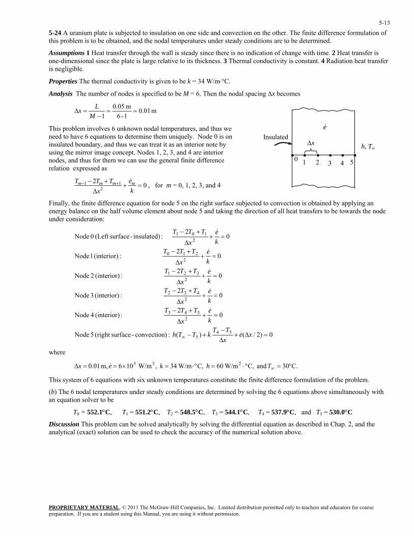
5-24 A uranium plate is subjected to insulation on one side and convection on the other. The finite difference formulation of this problem is to be obtained, and the nodal temperatures under steady conditions are to be determined.
Assumptions 1 Heat transfer through the wall is steady since there is no indication of change with time. 2 Heat transfer is one-dimensional since the plate is large relative to its thickness. 3 Thermal conductivity is constant. 4 Radiation heat transfer is negligible.
Properties The thermal conductivity is given to be k = 34 W/m⋅°C.
Analysis The number of nodes is specified to be M = 6. Then the nodal spacing ∆x becomes
m 01.01-61−M
This problem involves 6 unknown nodal temperatures, and thus we need to have 6 equations to determine them uniquely. Node 0 is oninsulated boundary, and thus we can treat it as an interior note by using the mirror image concept. Nodes 1, 2, 3, and 4 are interior nodes, and thus for the
m 05.0===∆
L
m we can use the general finite difference relation expressed as
x
022∆ kx
Finally, the finite difference equation for node 5 on the right surface subjected to convection is obtained by applying an energy balance on the
11 =++− +− eTTT mmmm &
, for m = 0, 1, 2, 3, and 4
half volume element about node 5 and taking the direction of all heat transfers to be towards the node er cons eration:
∆x
1•
e&
54••0 ••
3•2
Insulatedh, T∞
und id
0)2/()( :)convection -surface(right 5 Node
02
:(interior) 2 Node2
321 =++−
keTTT &
02
:(interior) 4 Node2
543 =++−
∆
keTTT
x&
02
:(interior) 3 Node2
432 =++−
keTTT &
02
:(interior) 1 Node
02
:insulated)-surface(Left 0 Node
545
210
2101
=∆+∆−
+−
∆
∆
=++−
=+∆
+−
∞ xexTT
kTTh
x
x
eTTTke
xTTT
&
&
&
where
This system of 6 equations with six unknown temperatures constitute the finite difference formulation of the problem.
(b) The 6 nodal temperatures under steady conditions are determined by solving the 6 equations above simultaneously with an equation solver to be
T0 = 552.1°C, T1 = 551.2°C, T2 = 548.5°C, T3 = 544.1°C, T4 = 537.9°C, and T5 = 530.0°C
Discussion This problem can be solved analytically by solving the differential equation as described in Chap. 2, and the analytical (exact) solution can be used to check the accuracy of the numerical solution above.
2∆ kx
C.30 and C, W/m60 C, W/m34 , W/m106 m, 01.0 235 °=°⋅=°⋅=×==∆ ∞Thkex &
PROPRIETARY MATERIAL. © 2011 The McGraw-Hill Companies, Inc. Limited distribution permitted only to teachers and educators for course preparation. If you are a student using this Manual, you are using it without permission.
5-14
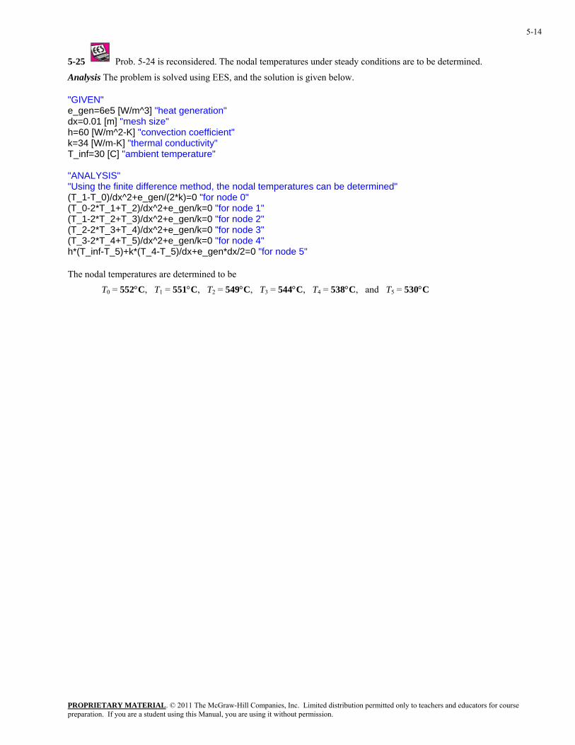
Prob. 5-24 is reconsidered. The nodal temperatures under steady5-25 conditions are to be determined.
nalysis is solved using EES, and the solution is given below.
nt"
peratures can be determined"
2=0 "for node 5"
The nodT0 = 552°C, T1 = 551°C, T2 = 549°C, T3 = 544°C, T4 = 538°C, and T5 = 530°C
A The problem "GIVEN" e_gen=6e5 [W/m^3] "heat generation" dx=0.01 [m] "mesh size" h=60 [W/m^2-K] "convection coefficiek=34 [W/m-K] "thermal conductivity" T_inf=30 [C] "ambient temperature" "ANALYSIS" "Using the finite difference method, the nodal tem(T_1-T_0)/dx^2+e_gen/(2*k)=0 "for node 0" (T_0-2*T_1+T_2)/dx^2+e_gen/k=0 "for node 1" (T_1-2*T_2+T_3)/dx^2+e_gen/k=0 "for node 2" (T_2-2*T_3+T_4)/dx^2+e_gen/k=0 "for node 3" (T_3-2*T_4+T_5)/dx^2+e_gen/k=0 "for node 4" h*(T_inf-T_5)+k*(T_4-T_5)/dx+e_gen*dx/
al temperatures are determined to be
PROPRIETARY MATERIAL. © 2011 The McGraw-Hill Companies, Inc. Limited distribution permitted only to teachers and educators for course preparation. If you are a student using this Manual, you are using it without permission.
5-15
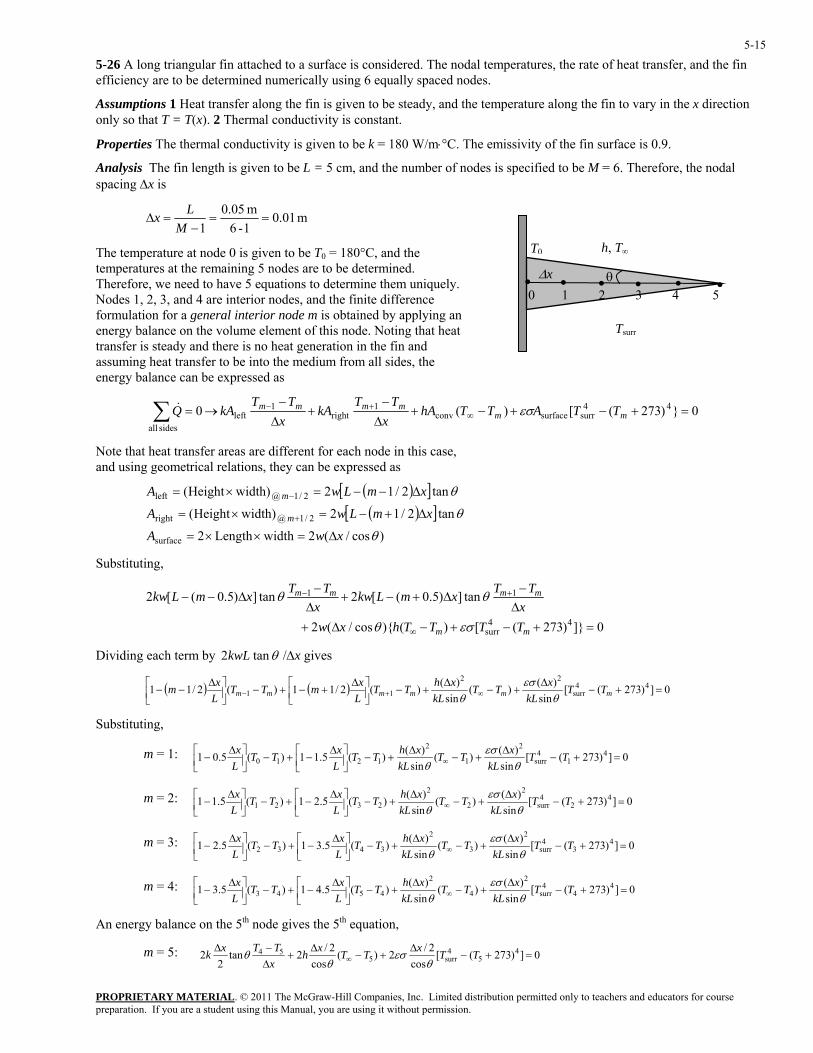
5-26 A long triangular fin attached to a surface is considered. The nodal temperatures, the rate of heat transfer, and the fin efficiency are to be determined numerically using 6 equally spaced nodes.
Assumptions 1 Heat transfer along the fin is given to be steady, and the temperature along the fin to vary in the x direction only so that T = T(x). 2 Thermal conductivity is constant.
Properties The thermal conductivity is given to be k = 180 W/m⋅°C. The emissivity of the fin surface is 0.9.
Analysis The fin length is given to be L = 5 cm, and the number of nodes is specified to be M = 6. Therefore, the nodal spacing ∆x is
m 01.01-6m 05.0
1==
−=∆
MLx
T0 h, T∞
θ ∆x • •• • ••0 1 2 3 4 5
Tsurr
The temperature at node 0 is given to be T0 = 180°C, and the temperatures at the remaining 5 nodes are to be determined. Therefore, we need to have 5 equations to determine them uniquely. Nodes 1, 2, 3, and 4 are interior nodes, and the finite difference formulation for a general interior node m is obtained by applying an energy balance on the volume element of this node. Noting that heat transfer is steady and there is no heat generation in the fin and assuming heat transfer to be into the medium from all sides, the energy balance can be expressed as
0})273([)( 0 44surrsurfaceconvrightleft
sides all ∆∆ xx
Note that heat transfer areas are different for each node in
11 =+−+−+−
+−
→= ∞+−
mmmmmm TTATThA
TTkA
TTkAQ εσ&
this case, and using geometrical relations, they can be expressed as
∑
( )[ ]( )[ ]
)cos/(2widthLength2
tan2/12width)Height(
tan2/12width)Height(
surfA ace
2/1@right
2/1@left
θ
θ
θ
xw
xmLwA
xmLwA
m
m
∆=××=
∆+−=×=
∆−−=×=
+
−
Substituting,
0]})273([)(){cos/(2
tan])5.0([2tan])5.0([2 1 −−− − mm TTmLkw θ
44surr
1
=+−+−∆+∆−
∆+−+∆
∆
∞
+
mm
mm
TTTThxwx
TTxmLkwx
x
εσθ
θ
Dividing each term by ∆x gives θtan2kwL /
( ) ( ) 0])273([sin
)()(sin
)()(2/11)(2/11 44surr
22
11 =+−∆
+−∆
+−⎥⎦⎤
⎢⎣⎡ ∆
+−+−⎥⎦⎤
⎢⎣⎡ ∆
−− ∞+− mmmmmm TTkL
xTTkL
xhTTLxmTT
Lxm
θεσ
θ
Substituting,
0])273([sin
)()(sin
)()(5.11)(5.01 41
4surr
2
1
2
1210 =+−∆
+−∆
+−⎥⎦⎤
⎢⎣⎡ ∆−+−⎥⎦
⎤⎢⎣⎡ ∆− ∞ TT
kLxTT
kLxhTT
LxTT
Lx
θεσ
θ m = 1:
0])273([sin
)()(sin
)()(5.21)(5.11 2321 +−⎥⎦⎤
⎢⎣⎡ −+−⎥⎦
⎤⎢⎣⎡ −
kTT
LTT
L4
24
surr
2
2
2=+−
∆+−
∆∆∆∞ TT
kLxTT
Lxhxx
θεσ
θ m = 2:
0])273([sin
)()(sin
)()(5.31)(5.21 43
4⎡m = 3: surr
2
3
2
3432 =+−∆
+−∆
+−⎥⎦⎤
⎢⎣⎡ ∆−+−⎥⎦
⎤⎢⎣
∆− ∞ TT
kLxTT
kLxhTT
LxTT
Lx
θεσ
θ
m = 4: 0])273([sin
)()(sin
)()(5.41)(5.31 44
4surr
2
4
2
4543 =+−∆
+−∆
+−⎥⎦⎤
⎢⎣⎡ ∆−+−⎥⎦
⎤⎢⎣⎡ ∆− ∞ TT
kLxTT
kLxhTT
LxTT
Lx
θεσ
θ
An energy balance on the 5th node gives the 5th equation,
m = 5: 0])273([cos
2/2)(cos
2/2tan2
2 45
4surr5
54 =+−∆
+−∆
+∆−∆
∞ TTxTTxhxTTxk
θεσ
θθ
PROPRIETARY MATERIAL. © 2011 The McGraw-Hill Companies, Inc. Limited distribution permitted only to teachers and educators for course preparation. If you are a student using this Manual, you are using it without permission.
5-16
4555
TTATThAQQ mm −++−== ∑∑∑ ∞ εσ&&
for the boundary nodes 0 and 5, and twice as large for the interior es 1, 2, , and 4, we have
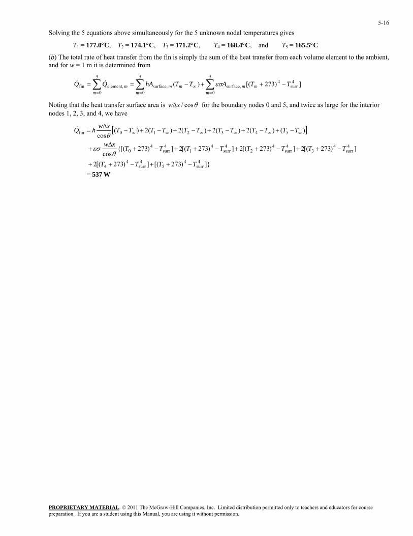
Solving the 5 equations above simultaneously for the 5 unknown nodal temperatures gives
T1 = 177.0°C, T2 = 174.1°C, T3 = 171.2°C, T4 = 168.4°C, and T5 = 165.5°C
(b) The total rate of heat transfer from the fin is simply the sum of the heat transfer from each volume element to the ambient, and for w = 1 m it is determined from
])273[()( 4surr
0 surface,
0 surface,
0 element,fin m
mm
mmm
===
Noting that the heat transfer surface area is θcos/xw∆nod 3
[ ]
W537=]})273[(])273[(2
])273[(2])273[(2])273[(2])273{[(cos
)()(2)(2)(2)(2)(cos
4surr
45
4surr
44
4surr
43
4surr
42
4surr
41
4surr
40
543210fin
TTTT
TTTTTTTTxw
TTTTTTTTTTTTxwhQ
−++−++
−++−++−++−+∆
+
−+−+−+−+−+−∆
= ∞∞∞∞∞∞
θεσ
θ&
PROPRIETARY MATERIAL. © 2011 The McGraw-Hill Companies, Inc. Limited distribution permitted only to teachers and educators for course preparation. If you are a student using this Manual, you are using it without permission.
5-17
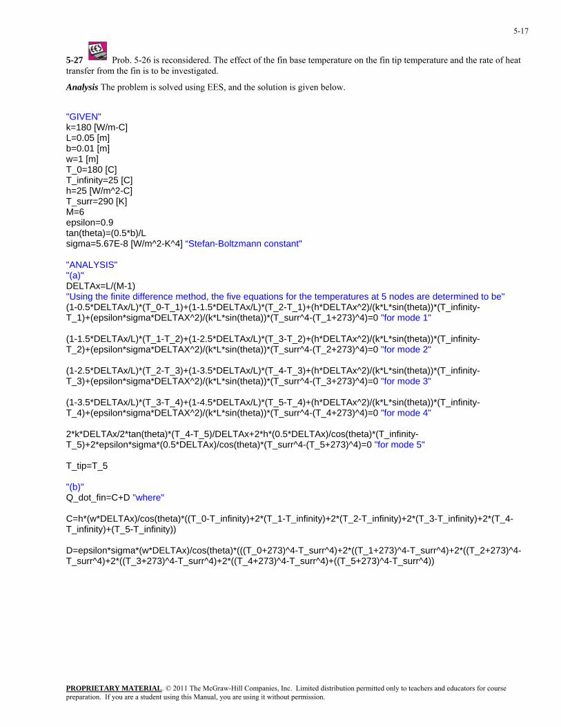
5-27 Prob. 5-26 is reconsidered. The effect of the fin base temperature on the fin tip temperature and the rate of heat transfer from the fin is to be investigated.
Analysis The problem is solved using EES, and the solution is given below.
"GIVEN" k=180 [W/m-C] L=0.05 [m] b=0.01 [m] w=1 [m] T_0=180 [C] T_infinity=25 [C] h=25 [W/m^2-C] T_surr=290 [K] M=6 epsilon=0.9 tan(theta)=(0.5*b)/L sigma=5.67E-8 [W/m^2-K^4] “Stefan-Boltzmann constant" "ANALYSIS" "(a)" DELTAx=L/(M-1) "Using the finite difference method, the five equations for the temperatures at 5 nodes are determined to be" (1-0.5*DELTAx/L)*(T_0-T_1)+(1-1.5*DELTAx/L)*(T_2-T_1)+(h*DELTAx^2)/(k*L*sin(theta))*(T_infinity-T_1)+(epsilon*sigma*DELTAX^2)/(k*L*sin(theta))*(T_surr^4-(T_1+273)^4)=0 "for mode 1" (1-1.5*DELTAx/L)*(T_1-T_2)+(1-2.5*DELTAx/L)*(T_3-T_2)+(h*DELTAx^2)/(k*L*sin(theta))*(T_infinity-T_2)+(epsilon*sigma*DELTAX^2)/(k*L*sin(theta))*(T_surr^4-(T_2+273)^4)=0 "for mode 2" (1-2.5*DELTAx/L)*(T_2-T_3)+(1-3.5*DELTAx/L)*(T_4-T_3)+(h*DELTAx^2)/(k*L*sin(theta))*(T_infinity-T_3)+(epsilon*sigma*DELTAX^2)/(k*L*sin(theta))*(T_surr^4-(T_3+273)^4)=0 "for mode 3" (1-3.5*DELTAx/L)*(T_3-T_4)+(1-4.5*DELTAx/L)*(T_5-T_4)+(h*DELTAx^2)/(k*L*sin(theta))*(T_infinity-T_4)+(epsilon*sigma*DELTAX^2)/(k*L*sin(theta))*(T_surr^4-(T_4+273)^4)=0 "for mode 4" 2*k*DELTAx/2*tan(theta)*(T_4-T_5)/DELTAx+2*h*(0.5*DELTAx)/cos(theta)*(T_infinity-T_5)+2*epsilon*sigma*(0.5*DELTAx)/cos(theta)*(T_surr^4-(T_5+273)^4)=0 "for mode 5" T_tip=T_5 "(b)" Q_dot_fin=C+D "where" C=h*(w*DELTAx)/cos(theta)*((T_0-T_infinity)+2*(T_1-T_infinity)+2*(T_2-T_infinity)+2*(T_3-T_infinity)+2*(T_4-T_infinity)+(T_5-T_infinity)) D=epsilon*sigma*(w*DELTAx)/cos(theta)*(((T_0+273)^4-T_surr^4)+2*((T_1+273)^4-T_surr^4)+2*((T_2+273)^4-T_surr^4)+2*((T_3+273)^4-T_surr^4)+2*((T_4+273)^4-T_surr^4)+((T_5+273)^4-T_surr^4))
PROPRIETARY MATERIAL. © 2011 The McGraw-Hill Companies, Inc. Limited distribution permitted only to teachers and educators for course preparation. If you are a student using this Manual, you are using it without permission.
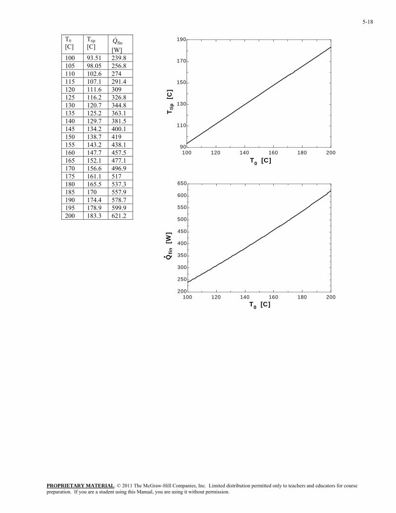
5-18
T0 [C]
Ttip [C]
finQ& [W]
100 93.51 239.8 105 98.05 256.8 110 102.6 274 115 107.1 291.4 120 111.6 309 125 116.2 326.8 130 120.7 344.8 135 125.2 363.1 140 129.7 381.5 145 134.2 400.1 150 138.7 419 155 143.2 438.1 160 147.7 457.5 165 152.1 477.1 170 156.6 496.9 175 161.1 517 180 165.5 537.3 185 170 557.9 190 174.4 578.7 195 178.9 599.9 200 183.3 621.2
100 120 140 160 180 20090
110
130
150
170
190
T0 [C]T t
ip [
C]
100 120 140 160 180 200200
250
300
350
400
450
500
550
600
650
T0 [C]
Qfin
[W
]
PROPRIETARY MATERIAL. © 2011 The McGraw-Hill Companies, Inc. Limited distribution permitted only to teachers and educators for course preparation. If you are a student using this Manual, you are using it without permission.
5-19
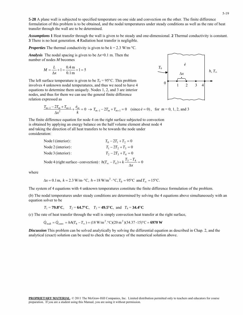
5-28 A plane wall is subjected to specified temperature on one side and convection on the other. The finite difference formulation of this problem is to be obtained, and the nodal temperatures under steady conditions as well as the rate of heat transfer through the wall are to be determined.
Assumptions 1 Heat transfer through the wall is given to be steady and one-dimensional. 2 Thermal conductivity is constant. 3 There is no heat generation. 4 Radiation heat transfer is negligible.
Properties The thermal conductivity is given to be k = 2.3 W/m⋅°C.
Analysis The nodal spacing is given to be ∆x=0.1 m. Then the number of nodes M becomes
T0
∆x
1
h, T∞
•
e&
40 • ••3
•2
51m 1.0m 4.01 =+=+
∆=
xLM
The left surface temperature is given to be T0 = 95°C. This problem involves 4 unknown nodal temperatures, and thus we need to have 4 equations to determine them uniquely. Nodes 1, 2, and 3 are interior nodes, and thus for them we can use the general finite difference relation expressed as
)0 (since 02 02 11 =++− +− eTT mmmm &
11 ==+−→ +− eTTTTmmm & , for m = 0, 1, 2, and 3
ut node 4
irection of all heat transfers to be towards the node under consideration:
2∆ kx
The finite difference equation for node 4 on the right surface subjected to convectionis obtained by applying an energy balance on the half volume element aboand taking the d
0)( :)convection -surface(right 4 Node
02 :(interior) 3 Node02 :(interior) 2 Node02 :(interior) 1 Node
434
432
321
210
=∆−
+−
=+−=+−=+−
∞ xTT
kTTh
TTTTTTTTT
where
tures under steady conditions are determined by solving the 4 equations above simultaneously with an equation
(c) The rate of heat transfer through the wall is simply convection heat transfer at the right surface,
ribed in Chap. 2, and the analytical (exact) solution can be used to check the accuracy of the numerical solution above.
C.15 and C95 C, W/m18 C, W/m3.2 m, 1.0 02 °=°=°⋅=°⋅==∆ ∞TThkx
The system of 4 equations with 4 unknown temperatures constitute the finite difference formulation of the problem.
(b) The nodal tempera solver to be
T1 = 79.8°C, T2 = 64.7°C, T3 = 49.5°C, and T4 = 34.4°C
W6970=°°=−== ∞ C15)-)(34.37m C)(20. W/m18()( 224convwall TThAQQ &&
Discussion This problem can be solved analytically by solving the differential equation as desc
PROPRIETARY MATERIAL. © 2011 The McGraw-Hill Companies, Inc. Limited distribution permitted only to teachers and educators for course preparation. If you are a student using this Manual, you are using it without permission.
5-20
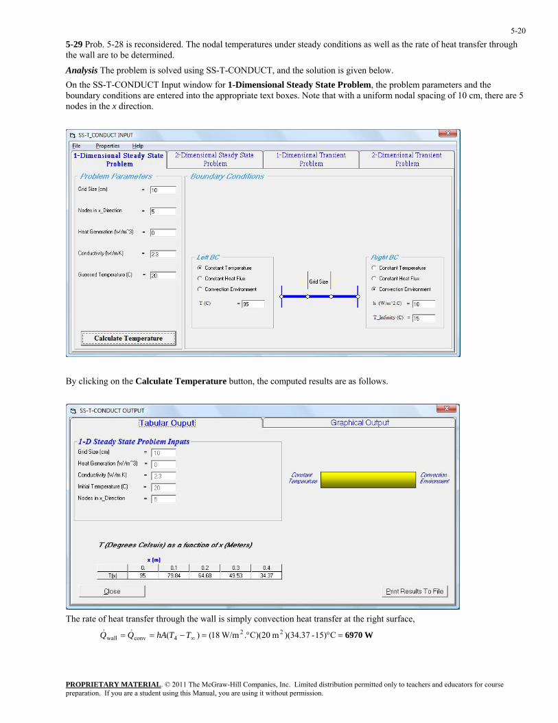
5-29 Prob. 5-28 is reconsidered. The nodal temperatures under steady conditions as well as the rate of heat transfer through the wall are to be determined.
Analysis The problem is solved using SS-T-CONDUCT, and the solution is given below. On the SS-T-CONDUCT Input window for 1-Dimensional Steady State Problem, the problem parameters and the boundary conditions are entered into the appropriate text boxes. Note that with a uniform nodal spacing of 10 cm, there are 5 nodes in the x direction.
By clicking on the Calculate Temperature button, the computed results are as follows.
The rate of heat transfer through the wall is simply convection heat transfer at the right surface,
W6970=°°=−== ∞ C15)-)(34.37m C)(20. W/m18()( 224convwall TThAQQ &&
PROPRIETARY MATERIAL. © 2011 The McGraw-Hill Companies, Inc. Limited distribution permitted only to teachers and educators for course preparation. If you are a student using this Manual, you are using it without permission.
5-21
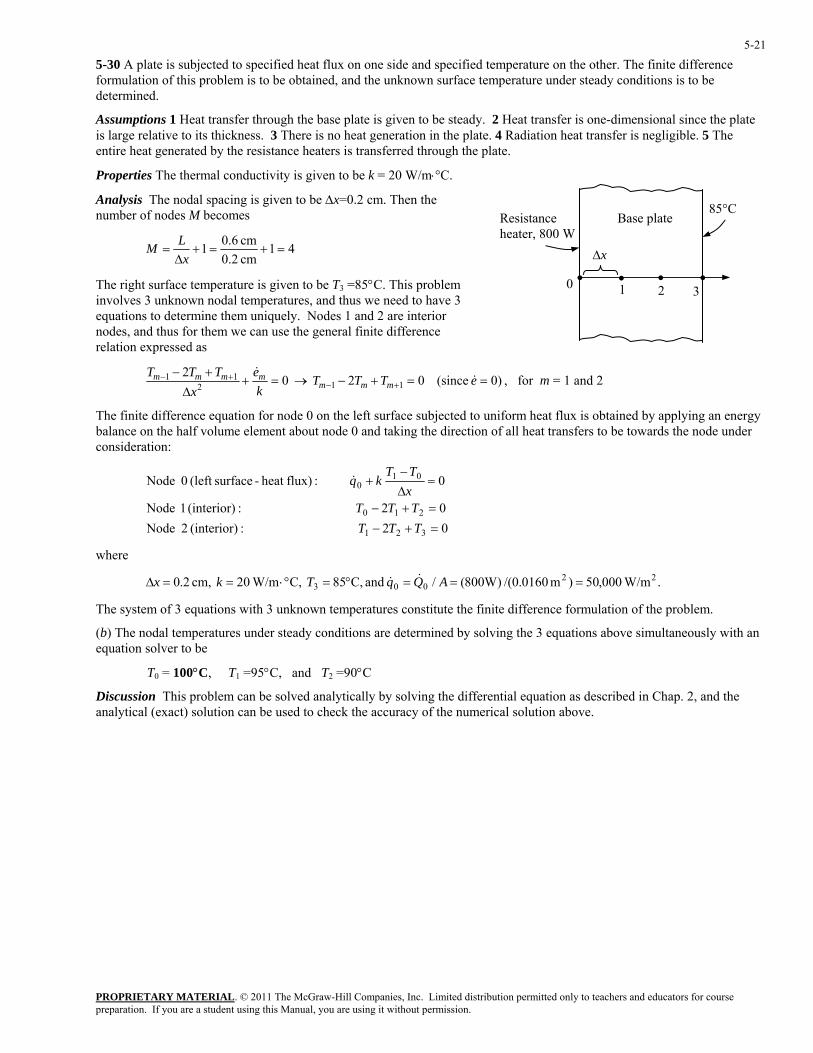
5-30 A plate is subjected to specified heat flux on one side and specified temperature on the other. The finite difference formulation of this problem is to be obtained, and the unknown surface temperature under steady conditions is to be determined.
Assumptions 1 Heat transfer through the base plate is given to be steady. 2 Heat transfer is one-dimensional since the plate is large relative to its thickness. 3 There is no heat generation in the plate. 4 Radiation heat transfer is negligible. 5 The entire heat generated by the resistance heaters is transferred through the plate.
Properties The thermal conductivity is given to be k = 20 W/m⋅°C.
Resistance heater, 800 W
∆x
Base plate
1
85°C
•0 • •3
•2
Analysis The nodal spacing is given to be ∆x=0.2 cm. Then the number of nodes M becomes
41cm 2.0cm 6.01 =+=+
∆=
xLM
The right surface temperature is given to be T3 =85°C. This problem involves 3 unknown nodal temperatures, and thus we need to have 3 equations to determine them uniquely. Nodes 1 and 2 are interior nodes, and thus for them we can use the general finite difference relation expressed as
)0 (since 02 02 11 ++− +− eTT mmmm &
112∆ +−kx mmm
The finite difference equation for node 0 on the left surface subjected to uniform heat flux is obtained by applying an energybalance on the h
==+−→= eTTTT& , for m = 1 and 2
alf volume element about node 0 and taking the direction of all heat transfers to be towards the node under
consideration:
02 :(interior) 2 Node02 :(interior) 1 Node
0 :flux)heat -surface(left 0 Node
321
210
010
=+−=+−
=∆−
+
TTTTTT
xTT
kq&
where
tures under steady conditions are determined by solving the 3 equations above simultaneously with an equation
cribed in Chap. 2, and the analytical (exact) solution can be used to check the accuracy of the numerical solution above.
. W/m000,50)m 0160.0/()W800(/ and C,85 C, W/m20 cm, 2.0 22003 ===°=°⋅==∆ AQqTkx &&
The system of 3 equations with 3 unknown temperatures constitute the finite difference formulation of the problem.
(b) The nodal tempera solver to be
T0 = 100°C, T1 =95°C, and T2 =90°C
Discussion This problem can be solved analytically by solving the differential equation as des
PROPRIETARY MATERIAL. © 2011 The McGraw-Hill Companies, Inc. Limited distribution permitted only to teachers and educators for course preparation. If you are a student using this Manual, you are using it without permission.
5-22
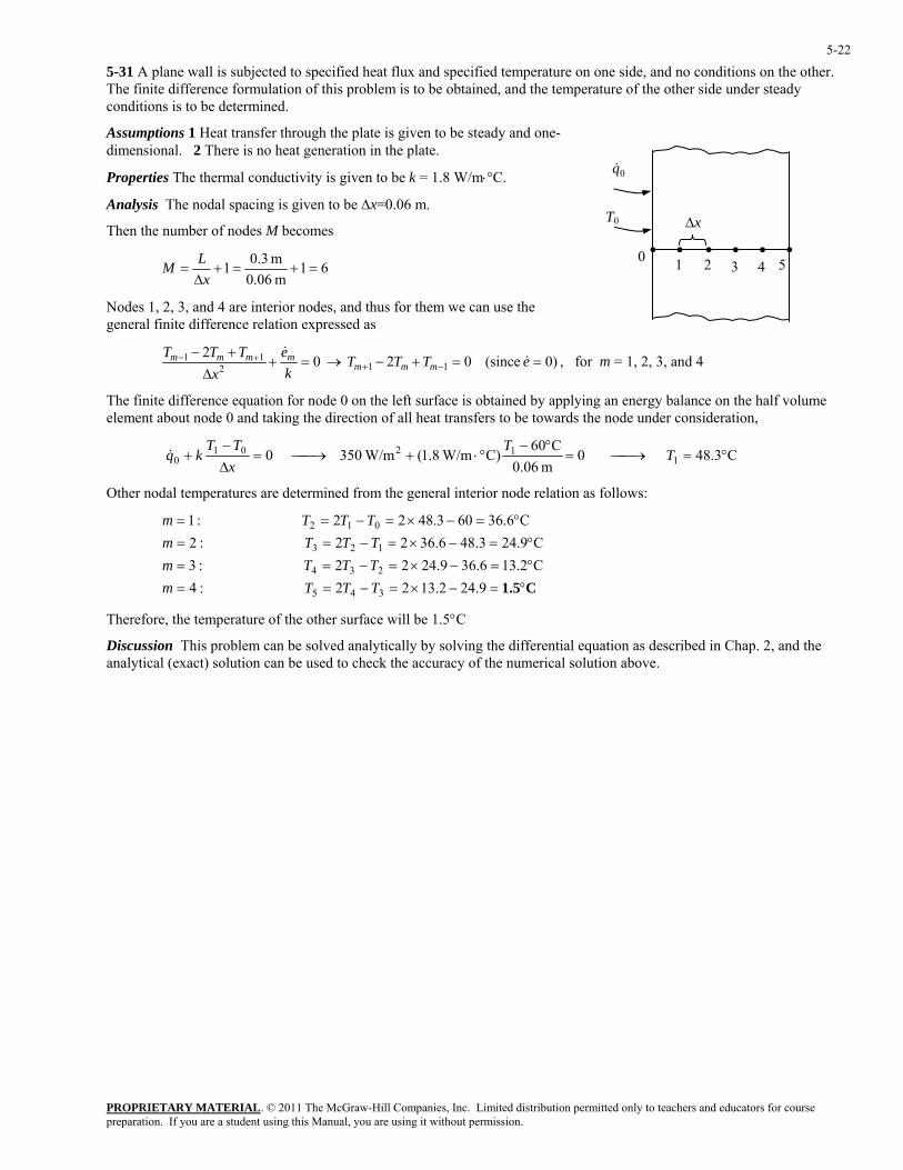
5-31 A plane wall is subjected to specified heat flux and specified temperature on one side, and no conditions on the other. The finite difference formulation of this problem is to be obtained, and the temperature of the other side under steady conditions is to be determined.
Assumptions 1 Heat transfer through the plate is given to be steady and one-dimensional. 2 There is no heat generation in the plate.
∆x
1•
0q&
T0
54•0 • ••
3•2
Properties The thermal conductivity is given to be k = 1.8 W/m⋅°C.
Analysis The nodal spacing is given to be ∆x=0.06 m.
Then the number of nodes M becomes
61m 06.0
m 3.01 =+=+∆
=x
LM
Nodes 1, 2, 3, and 4 are interior nodes, and thus for them we can use the general finite difference relation expressed as
)0 (since 02 02 11 =++− +− eTT mmmm &
112∆ kx mmm
The finite difference equation for node 0 on the left surface is obtained by applying an energy balance on the ha
==+−→ −+ eTTTT& , for m = 1, 2, 3, and 4
lf volume element about node 0 and taking the direction of all heat transfers to be towards the node under consideration,
C3.48 0 m0.060 ∆
C60C) W/m8.1( W/m350 0 1
1201 °=⎯→⎯=°−
°⋅+⎯→⎯=−
+ TT
xTT
kq&
ther noda temperatures are determined from the general interior node relation as follows:
°=°=
9.242.1322 :4
C6.36
345 TTTm
Therefore, the temperature of the other surface will be 1.5°C
Discussion This problem can be solved analytically by solving the differential equation as described in Chap. 2, and the analytical (exact) solution can be used to check the accuracy of the numerical solution above.
O l
°=−×=−==
=C2.136.369.2422 :3C9.243.486.3622 :2
234
123
TTTmTTTm
−×=−=−×=−== 603.4822 :1 012 TTTm
C1.5°=−×=−==
PROPRIETARY MATERIAL. © 2011 The McGraw-Hill Companies, Inc. Limited distribution permitted only to teachers and educators for course preparation. If you are a student using this Manual, you are using it without permission.
5-23
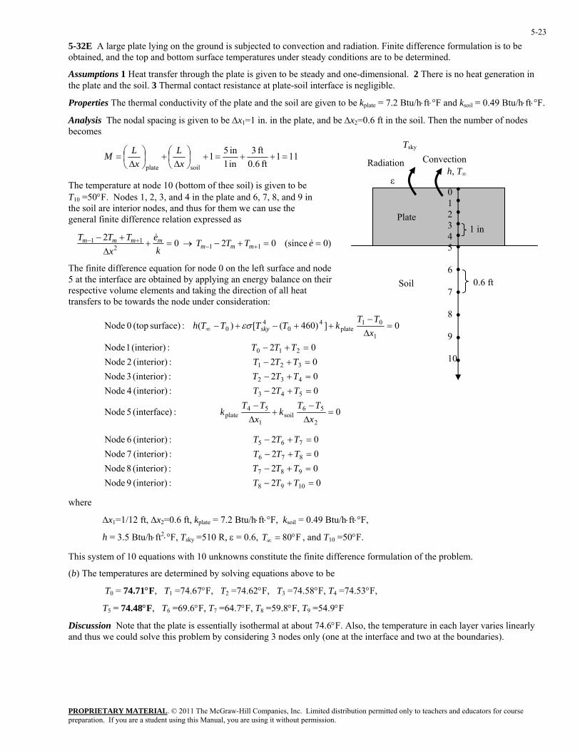
5-32E A large plate lying on the ground is subjected to convection and radiation. Finite difference formulation is to be obtained, and the top and bottom surface temperatures under steady conditions are to be determined.
Assumptions 1 Heat transfer through the plate is given to be steady and one-dimensional. 2 There is no heat generation in the plate and the soil. 3 Thermal contact resistance at plate-soil interface is negligible.
Properties The thermal conductivity of the plate and the soil are given to be kplate = 7.2 Btu/h⋅ft⋅°F and ksoil = 0.49 Btu/h⋅ft⋅°F.
Analysis The nodal spacing is given to be ∆x1=1 in. in the plate, and be ∆x2=0.6 ft in the soil. Then the number of nodes becomes
Tsky
111ft 0.6
ft 3in 1in 51
soilplate=++=+⎟
⎠⎞
⎜⎝⎛∆
+⎟⎠⎞
⎜⎝⎛∆
=x
Lx
LM
The temperature at node 10 (bottom of thee soil) is given to be T10 =50°F. Nodes 1, 2, 3, and 4 in the plate and 6, 7, 8, and 9 in the soil are interior nodes, and thus for them we can use the general finite difference relation expressed as
)0 (since 02 02112
11 ==+−→=+∆ kx
The finite difference equation for node 0 on the left surface and node 5 at the interface are obtained by applying an energy balance onrespective volume elements and taking the direction of
+−+−
+ eTTTeTTTmmm
mmm &&
their all heat
transfers to be towards the node under consideration:
−m
0 :)(interface 5 Node
02 :(interior) 4 Node02 :(interior) 3 Node02 :(interior) 2 Node02 :(interior) 1 Node
0])460([)( :surface) (top 0 Node
2
56soil
1
54plate
543
432
321
210
1
01plate
40
40
=∆−
+∆−
=+−=+−=+−=+−
=∆−
++−+−∞
xTT
kx
TTk
TTTTTTTTTTTT
xTT
kTTTTh skyεσ
Convection
εh, T∞
0.6 ftSoil
Radiation
• • • • • •10
• • • • •
0 1 2 3 4 5 6 7 8 9
Plate1 in
0 :(interior) 9 Node 8
7
=T02 :(interior) 8 Node02 :(interior) 7 Node 876
=+−=−
TTTTTT
2
02 :(interior) 6 Node
109
98
765
+−
+=+−
TT
TTT
h⋅ft⋅°F,
where
∆x1=1/12 ft, ∆x2=0.6 ft, kplate = 7.2 Btu/h⋅ft⋅°F, ksoil = 0.49 Btu/
h = 3.5 Btu/h⋅ft2⋅°F, Tsky =510 R, ε = 0.6, F80°=∞T , and T10 =50°F.
This system of 10 equations with 10 unknowns constitute the finite difference formulation of the problem.
T0 = 74.71°F, T1 =74.67°F, T2 =74.62°F, T3 =74.58°F, T4 =74.53°F,
T5 = 74.48°F, T6 =69.6°F, T7 =64.7°F, T8 =59.8°F, T9 =54.9°F
Discussion Note that the plate is essentially isothermal at about 74.6°F. Also, the temperature in each layer varies linearly and thus we could solve this problem by considering 3 nodes only (one at the interface and two at the boundaries).
(b) The temperatures are determined by solving equations above to be
PROPRIETARY MATERIAL. © 2011 The McGraw-Hill Companies, Inc. Limited distribution permitted only to teachers and educators for course preparation. If you are a student using this Manual, you are using it without permission.
5-24
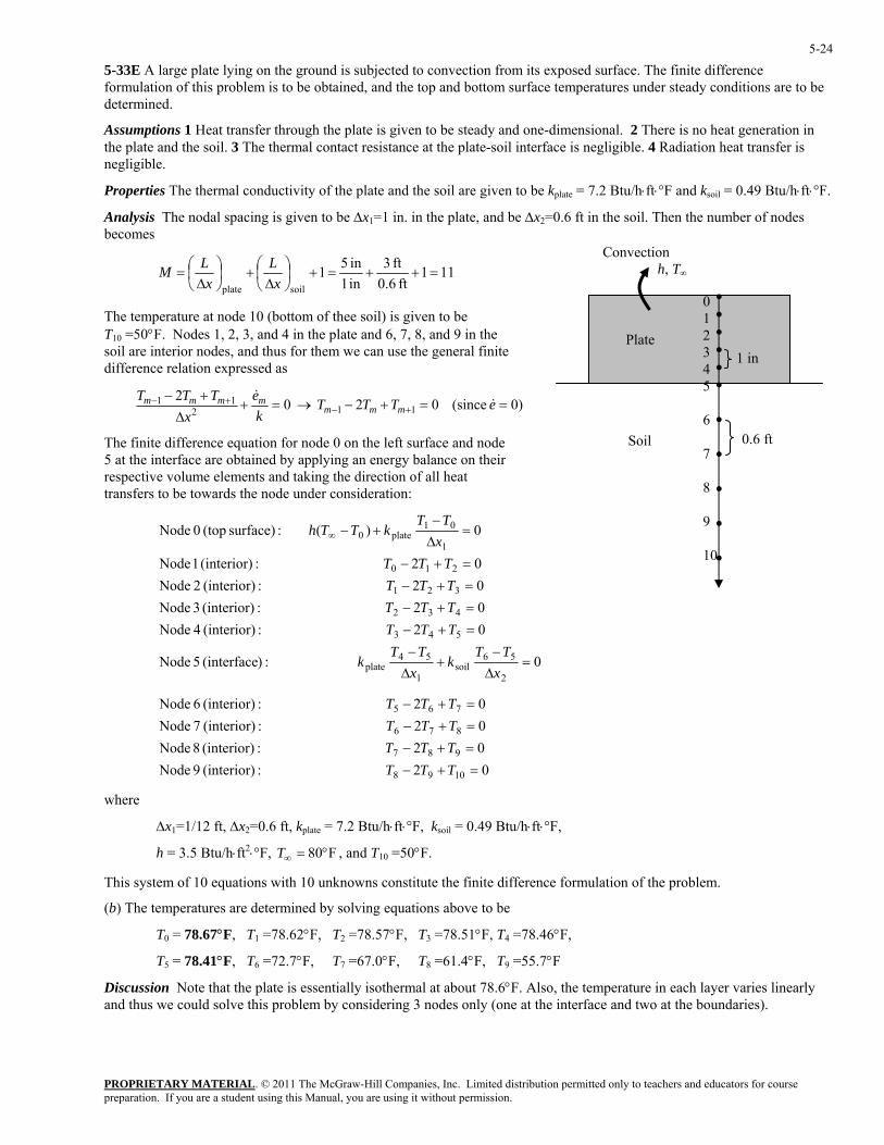
5-33E A large plate lying on the ground is subjected to convection from its exposed surface. The finite difference formulation of this problem is to be obtained, and the top and bottom surface temperatures under steady conditions are to be determined.
Assumptions 1 Heat transfer through the plate is given to be steady and one-dimensional. 2 There is no heat generation in the plate and the soil. 3 The thermal contact resistance at the plate-soil interface is negligible. 4 Radiation heat transfer is negligible.
Properties The thermal conductivity of the plate and the soil are given to be kplate = 7.2 Btu/h⋅ft⋅°F and ksoil = 0.49 Btu/h⋅ft⋅°F.
Analysis The nodal spacing is given to be ∆x1=1 in. in the plate, and be ∆x2=0.6 ft in the soil. Then the number of nodes becomes
111ft 0.6in 1soilplate ⎠⎝ ∆⎠⎝ ∆ xx
The temperature at node 10 (bottom of thee soil) is given to be T
ft 3in 51 =++=+⎟⎞
⎜⎛+⎟
⎞⎜⎛=
LLM
hem we can use the general finite ence relation expressed as
10 =50°F. Nodes 1, 2, 3, and 4 in the plate and 6, 7, 8, and 9 in the soil are interior nodes, and thus for tdiffer
)0 (since 02 0 112 ==+−→=+∆ +− eTTT
kx mmm &
The finite difference equation for node 0 on the left surface and node 5 at the interface are obtained by applying an energy balance onrespective volume elements and taking the direction of al
2 11 +− +− eTTT mmmm &
their l heat
transfers to e towards the node under consideration: b
0 :)(interface 5 Node platek
02 :(interior) 4 Node02 :(interior) 3 Node02 :(interior) 2 Node02 :(interior) 1 Node
0)( :surface) (top 0 Node
2
56soil
1
54
432
321
210
1
01plate0
=∆
+∆
=+−=+−=+−=+−
=∆−
+−∞
xk
x
TTTTTTTTTTTT
xTT
kTTh
h = 3.5 Btu/h⋅ft2⋅°F, , and T10 =50°F.
This system of 10 equations with 10 unknowns constitute the finite difference formulation of the problem.
(b) The temperatures are determined by solving equations above to be
T0 = 78.67°F, T1 =78.62°F, T2 =78.57°F, T3 =78.51°F, T4 =78.46°F,
T5 = 78.41°F, T6 =72.7°F, T7 =67.0°F, T8 =61.4°F, T9 =55.7°F
Discussion Note that the plate is essentially isothermal at about 78.6°F. Also, the temperature in each layer varies linearly and thus we could solve this problem by considering 3 nodes only (one at the interface and two at the boundaries).
Convectionh, T∞
0.6 ftSoil
• • • • • •
•••••
0 1 2 3 4 5 6 7 8 9 10
1 inPlate
543
−− TTTT
02 :(interior) 6 Node 765 =+− TTT
02 :(interior) 8 Node 987 =+− TTT02 :(interior) 7 Node 876 =+− TTT
02 :(interior) 9 Node 1098 =+− TTT
where
∆x1=1/12 ft, ∆x2=0.6 ft, kplate = 7.2 Btu/h⋅ft⋅°F, ksoil = 0.49 Btu/h⋅ft⋅°F,
F80°=∞T
PROPRIETARY MATERIAL. © 2011 The McGraw-Hill Companies, Inc. Limited distribution permitted only to teachers and educators for course preparation. If you are a student using this Manual, you are using it without permission.
5-25
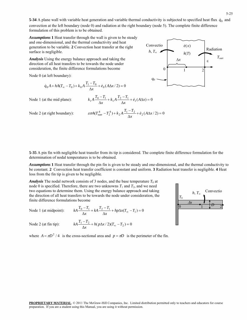
5-34 A plane wall with variable heat generation and variable thermal conductivity is subjected to specified heat flux and convection at the left boundary (node 0) and radiation at the right boundary (node 5). The complete finite difference formulation of this problem is to be obtained.
0q&
Assumptions 1 Heat transfer through the wall is given to be steady and one-dimensional, and the thermal conductivity and heat generation to be variable. 2 Convection heat transfer at the right surface is negligible.
Convectio
∆x
1
ε
k(T)
)(xe& h, T∞
Radiation
Tsurr
q0
20 •••
Analysis Using the energy balance approach and taking the direction of all heat transfers to be towards the node under consideration, the finite difference formulations become
Node 0 (at left boundary):
0)2/()( 001
000 =∆+∆−
+−+ ∞ xAexTT
AkTThAAq &&
0)(112
110
1 =∆+∆−
+∆−
xAexTT
AkxTT
Ak & Node 1 (at the mid plane):
0)2/()( 221
24
24
surr =∆+∆−
+− xAexTT
AkTTA &εσ Node 2 (at right boundary):
5-35 A pin fin with negligible heat transfer from its tip is considered. The complete finite difference formulation for the determination of nodal temperatures is to be obtained.
Assumptions 1 Heat transfer through the pin fin is given to be steady and one-dimensional, and the thermal conductivity to diation heat transfer is negligible. 4 Heat
the energy balance approach and taking the direction of all heat transfers to be towards the node under consideration, the
lations become
be constant. 2 Convection heat transfer coefficient is constant and uniform. 3 Raloss from the fin tip is given to be negligible.
Analysis The nodal network consists of 3 nodes, and the base temperature T0 at node 0 is specified. Therefore, there are two unknowns T1 and T2, and we need two equations to determine them. Using Convectio
T0
, Th ∞
• ••0 1 2D∆xfinite difference formu
0)( 11210 =−∆+
∆−
+∆−
∞ TTxhpxTT
kAxTT
kNode 1 (at midpoint): A
Node 2 (at fin tip): 0))(2/( 221 =−∆+
∆−TT
∞ TTxphx
kA
where is the cross-sectional area and 4/2DA π= Dp π= is the perimeter of the fin.
PROPRIETARY MATERIAL. © 2011 The McGraw-Hill Companies, Inc. Limited distribution permitted only to teachers and educators for course preparation. If you are a student using this Manual, you are using it without permission.
5-26
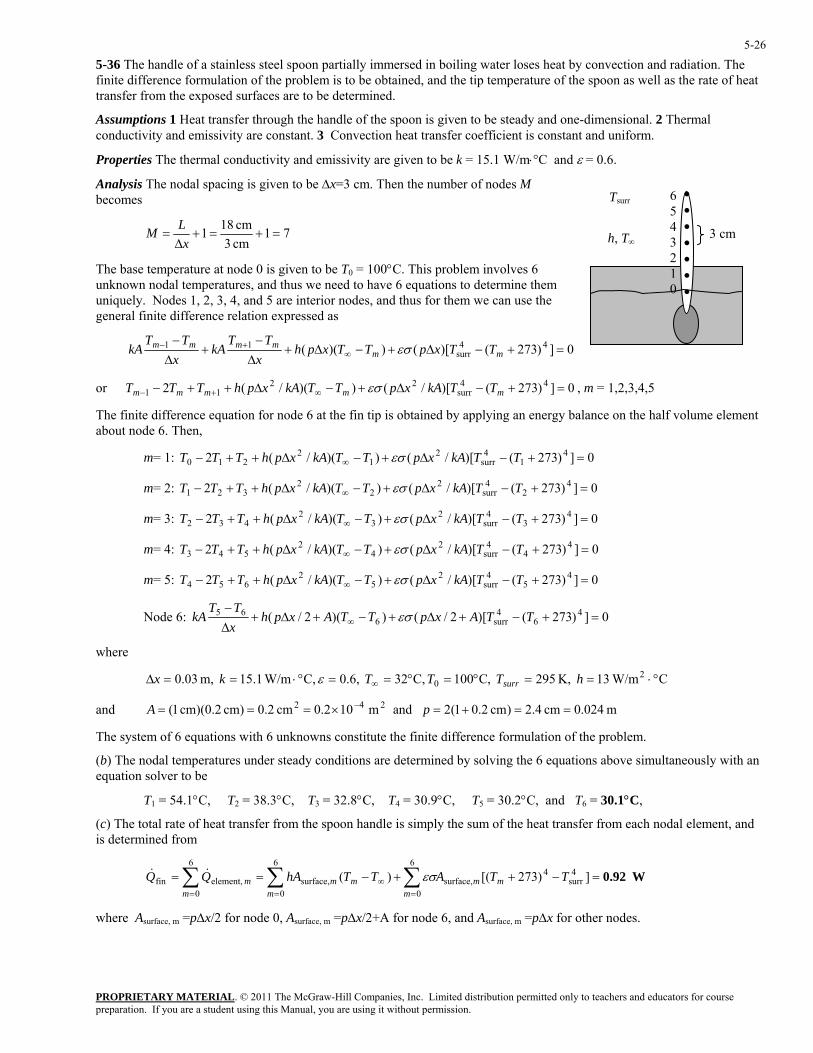
5-36 The handle of a stainless steel spoon partially immersed in boiling water loses heat by convection and radiation. The finite difference formulation of the problem is to be obtained, and the tip temperature of the spoon as well as the rate of heat transfer from the exposed surfaces are to be determined.
Assumptions 1 Heat transfer through the handle of the spoon is given to be steady and one-dimensional. 2 Thermal conductivity and emissivity are constant. 3 Convection heat transfer coefficient is constant and uniform.
Properties The thermal conductivity and emissivity are given to be k = 15.1 W/m⋅°C and ε = 0.6.
Analysis The nodal spacing is given to be ∆x=3 cm. Then the number of nodes M becomes
71cm 3cm 181 =+=+
∆=
xLM
The base temperature at node 0 is given to be T0 = 100°C. This problem involves 6 unknown nodal temperatures, and thus we need to have 6 equations to determine them uniquely. Nodes 1, 2, 3, 4, and 5 are interior nodes, and thus for them we can use the general finite difference relation expressed as
0])273()[())(( 44surr
11 =+−∆+−∆+∆−
+∆−
∞+−
mmmmmm TTxpTTxph
xTT
kAx
TTkA εσ
22
equation for node 6 at the fin tip is obtained by applying an energy balance on the half volume element about node 6. Then,
εσ
∞ TTkAxpTTkAxphTTT εσ
εσ
=+−∆+−∆++ ∞ TTkAxpTTkAxphTTT εσ
=+−∆+−∆++− ∞ TTkAxpTTkAxphTT εσ
Node 6:
h, T∞
Tsurr 6543210
3 cm
•••••••
or 0])273()[/())(/(2 surr11 =+−∆+−∆++− ∞+− mmmmm TTkAxpTTkAxphTTT εσ , m = 1,2,3,4,5
The finite difference
44
m= 1: T 0])273()[/())(/(2 41
4surr
21
2210 =+−∆+−∆++− ∞ TTkAxpTTkAxphTT
m= 2: − 0])273()[/())(/(2 42
4surr
22
2321 =+−∆+−∆++
m= 3: T 0])273()[/())(/(2 43
4surr
23
2432 =+−∆+−∆++− ∞ TTkAxpTTkAxphTT
0])273()[/())(/(2 44
4surr
24
254m= 4: 3 −
0])273()[/())(/(2 45
4surr
25
265m= 5: 4T
0])273()[2/())(2/( 46
4surr6
65 =+−+∆+−+∆+∆−
∞ TTAxpTTAxphxTT
kA εσ
where
The n ultaneously with an ion sol
2 3 4 5 6
(c) The total rate of heat transfer from the spoon handle is simply the sum of the heat transfer from each nodal element, and is determin d from
0surface,
0surface,
0 element,fin TTATThAQQ m
mm
mmm
mm εσ&&
where Asurface, m =p∆x/2 for node 0, Asurface, m =p∆x/2+A for node 6, and Asurface, m =p∆x for other nodes.
C W/m13 K, 295 ,C100 C,32 0.6, C, W/m1.15 m, 03.0 20 °⋅==°=°==°⋅==∆ ∞ hTTTkx surrε
and m 0.024cm 4.2)cm 2.01(2 and m 102.0 cm 0.2cm) cm)(0.2 1( 242 ==+=×=== − pA
The system of 6 equations with 6 unknowns constitute the finite difference formulation of the problem.
(b) odal temperatures under steady conditions are determined by solving the 6 equations above simequat ver to be
T1 = 54.1°C, T = 38.3°C, T = 32.8°C, T = 30.9°C, T = 30.2°C, and T = 30.1°C,
e
W0.92=−++−== ∑∑∑==
∞=
])273[()( 4surr
4666
PROPRIETARY MATERIAL. © 2011 The McGraw-Hill Companies, Inc. Limited distribution permitted only to teachers and educators for course preparation. If you are a student using this Manual, you are using it without permission.
5-27
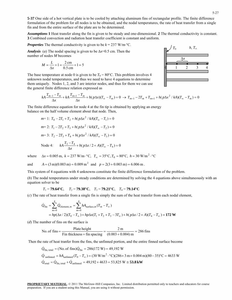
5-37 One side of a hot vertical plate is to be cooled by attaching aluminum fins of rectangular profile. The finite difference formulation of the problem for all nodes is to be obtained, and the nodal temperatures, the rate of heat transfer from a single fin and from the entire surface of the plate are to be determined.
Assumptions 1 Heat transfer along the fin is given to be steady and one-dimensional. 2 The thermal conductivity is constant. 3 Combined convection and radiation heat transfer coefficient is constant and uniform.
Properties The thermal conductivity is given to be k = 237 W/m⋅°C. T0 h, T∞
∆x• • • • •
0 1 2 3 4
Analysis (a) The nodal spacing is given to be ∆x=0.5 cm. Then the number of nodes M becomes
51cm 5.0
cm 21 =+=+∆
=x
LM
The base temperature at node 0 is given to be T0 = 80°C. This problem involves 4 unknown nodal temperatures, and thus we need to have 4 equations to determine them uniquely. Nodes 1, 2, and 3 are interior nodes, and thus for them we can use the general finite difference relation expressed as
0))((11 =−∆+∆∆ xx
The finite difference equation for node 4 at the fin tip is obt
−+
−∞
+m
mmm TTxphTT
kAT
k
ained by applying an energy balance on t volume element about that node. Then,
m= 3: =−∆++− ∞ TTkAxphTTT
Node 4:
−mTA → 0))(/(2 2
11 =−∆++− ∞+− mmmm TTkAxphTTT
he half
m= 1: 0))(/(2 12
210 =−∆++− ∞ TTkAxphTTT
0))(/(2 22
321 =−∆++− ∞ TTkAxphTTT m= 2:
0))(/(2 32
432
0))(2/( 443 =−+∆+
∆−
∞ TTAxphxTT
kA
where
ined bove simultaneously with an equation
(c) The rate of heat transfer from a single fin is simply the sum of the heat transfer from each nodal element,
0surface,
0 element,fin
TTAxphTTTTxhpTTxhp
TThAQQm
mmm
m
C W/m30 C,80 C,35 C, W/m237 m, 005.0 20 °⋅=°=°=°⋅==∆ ∞ hTTkx
and m 006.6)m 003.03(2 and m 0.009m) m)(0.003 3( 2 =+=== pA .
This system of 4 equations with 4 unknowns constitute the finite difference formulation of the problem.
(b) The nodal temperatures under steady conditions are determ by solving the 4 equations a solver to be
T1 = 79.64°C, T2 = 79.38°C, T3 = 79.21°C, T4 = 79.14°C
W172=−+∆+−++∆+−∆=
−==
∞∞∞
=∞
=∑∑
))(2/()3())(2/(
)(
43210
44&&
(d) The number of fins on the surface is
fins 286m 0.004) (0.003
m 2spacingfin essFin thickn
height Plate fins of No. =+
=+
=
Then the rate of heat tranfer from the fins, the unfinned portion, and the entire finned surface become
kW 53.8≅=+=+=
=°−××°⋅=−=
===
∞
W53,8254633192,49
W4633C35)m)(80 0.004 m 3C)(286 W/m30()(
W,19249 W)172(286)fins of No.(
unfinned totalfin,total
20unfinned`unfinned
fin totalfin,
QQQ
TThAQ
&&&
&
&&
PROPRIETARY MATERIAL. © 2011 The McGraw-Hill Companies, Inc. Limited distribution permitted only to teachers and educators for course preparation. If you are a student using this Manual, you are using it without permission.
5-28
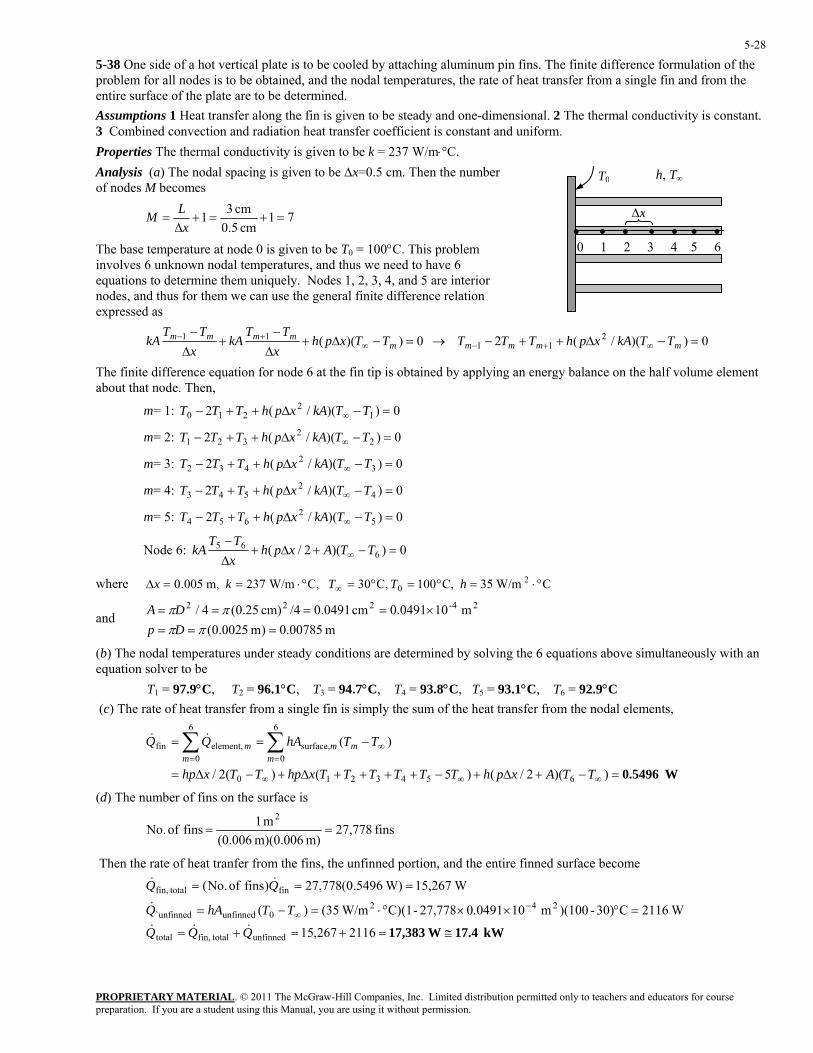
5-38 One side of a hot vertical plate is to be cooled by attaching aluminum pin fins. The finite difference formulation of the problem for all nodes is to be obtained, and the nodal temperatures, the rate of heat transfer from a single fin and from the entire surface of the plate are to be determined. Assumptions 1 Heat transfer along the fin is given to be steady and one-dimensional. 2 The thermal conductivity is constant. 3 Combined convection and radiation heat transfer coefficient is constant and uniform. Properties The thermal conductivity is given to be k = 237 W/m⋅°C. Analysis (a) The nodal spacing is given to be ∆x=0.5 cm. Then the number of nodes M becomes
T0 h, T∞
∆x• • • • • • • 0 1 2 3 4 5 6
71cm 5.0
cm 31 =+=+∆
=x
LM
The base temperature at node 0 is given to be T0 = 100°C. This problem involves 6 unknown nodal temperatures, and thus we need to have 6 equations to determine them uniquely. Nodes 1, 2, 3, 4, and 5 are interior nodes, and thus for them we can use the general finite difference relation expressed as
0))((11−mTA =−∆+
−+
−∞
+m
mmm TTxphTT
kAT
k →
uation for node 6 at the fin tip is obtained by applying an energy balance on the half volume element about tha T en,
=−∆++− ∞ TTkAxphTT
Node 6:
0))(/(2 211 =−∆++− ∞+− mmmm TTkAxphTTT
∆∆ xxThe finite difference eq
t node. h
m= 1: 0))(/(2 12
210 =−∆++− ∞ TTkAxphTTT
0))(/(2 22
321 =−∆++− ∞ TTkAxphTTT m= 2:
m= 3: 0))(/(2 32
432 =−∆++− ∞ TTkAxphTTT
0))(/(2 42
543 =−∆++− ∞ TTkAxphTTT m= 4:
m= 5: 4T 0))(/(2 52
65
0))(2/( 665 =−+∆+
∆−
∞ TTAxphxTT
kA
e 5 C,100 C,30 C, W/m237 m, 005.0 20 °⋅=°=°=°⋅==∆ ∞ hTTkx
×==== ππDA
simultaneously with an
2 3 4 5 6
he ra of heat transfer from a single fin is simply the sum of the heat transfer from the nodal elements,
=
∞=
∑∑))(2/()5()(2/
)(0
surface,0
element,fin
TTAxphTTTTTTxhpTTxhp
TThAQQm
mmm
m&&
wher 3 C W/m
and m 00785.0)m 0025.0( === ππDp
m 100.0491cm 0491.0/4cm) 25.0(4/ 2-4222
(b) The nodal temperatures under steady conditions are determined by solving the 6 equations aboveequation solver to be 1 T = 97.9°C, T = 96.1°C, T = 94.7°C, T = 93.8°C, T = 93.1°C, T = 92.9°C (c) T te
W0.5496=−+∆+−++++∆+−∆=
−==66
∞∞∞ 6543210
ber of fins on the surface is (d) The num
fins 778,27m) m)(0.006 (0.006
m 1 fins of No.2
==
Then the rate of heat tranfer from the fins, the unfinned portion, and the entire finned surface become
kW 17.4 W17,383 ≅=+=+=
=°××°⋅=−=
===−
∞
2116267,15
W2116C30)-)(100m 10 0491.027,778-C)(1 W/m35()(
W15,267 W)5496.0(778,27)fins of No.(
unfinned totalfin,total
2420unfinned`unfinned
fin totalfin,
QQQ
TThAQ
&&&
&
&&
PROPRIETARY MATERIAL. © 2011 The McGraw-Hill Companies, Inc. Limited distribution permitted only to teachers and educators for course preparation. If you are a student using this Manual, you are using it without permission.
5-29
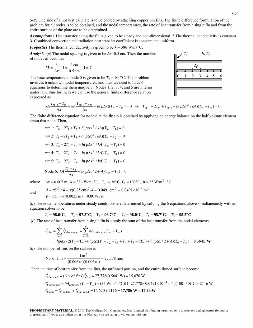
5-39 One side of a hot vertical plate is to be cooled by attaching copper pin fins. The finite difference formulation of the problem for all nodes is to be obtained, and the nodal temperatures, the rate of heat transfer from a single fin and from the entire surface of the plate are to be determined. Assumptions 1 Heat transfer along the fin is given to be steady and one-dimensional. 2 The thermal conductivity is constant. 3 Combined convection and radiation heat transfer coefficient is constant and uniform. Properties The thermal conductivity is given to be k = 386 W/m⋅°C. Analysis (a) The nodal spacing is given to be ∆x=0.5 cm. Then the number of nodes M becomes
T0 h, T∞
∆x• • • • • • • 0 1 2 3 4 5 6
71cm 5.0
cm 31 =+=+∆
=x
LM
The base temperature at node 0 is given to be T0 = 100°C. This problem involves 6 unknown nodal temperatures, and thus we need to have 6 equations to determine them uniquely. Nodes 1, 2, 3, 4, and 5 are interior nodes, and thus for them we can use the general finite difference relation expressed as
0))((11−mTA =−∆+
−+
−∞
+m
mmm TTxphTT
kAT
k →
uation for node 6 at the fin tip is obtained by applying an energy balance on the half volume element about tha T en,
=−∆++− ∞ TTkAxphTT
Node 6:
0))(/(2 211 =−∆++− ∞+− mmmm TTkAxphTTT
∆∆ xxThe finite difference eq
t node. h
m= 1: 0))(/(2 12
210 =−∆++− ∞ TTkAxphTTT
0))(/(2 22
321 =−∆++− ∞ TTkAxphTTT m= 2:
m= 3: 0))(/(2 32
432 =−∆++− ∞ TTkAxphTTT
0))(/(2 42
543 =−∆++− ∞ TTkAxphTTT m= 4:
m= 5: 4T 0))(/(2 52
65
0))(2/( 665 =−+∆+
∆−
∞ TTAxphxTT
kA
5 C,100 C,30 C, W/m386 m, 005.0 20 °⋅=°=°=°⋅==∆ ∞ hTTkx
×==== ππDA
(b) The n e simultaneously with an
1 2 3 4 5 6
he ra of heat transfer from a single fin is simply the sum of the heat transfer from the nodal elements,
=
∞=
∑∑))(2/()5()(2/
)(0
surface,0
element,fin
TTAxphTTTTTTxhpTTxhp
TThAQQm
mmm
m&&
where 3 C W/m
and m 00785.0)m 0025.0( === ππDp
m 100.0491cm 0491.0/4cm) 25.0(4/ 2-4222
odal temperatures under steady conditions are determined by solving the 6 equations abov solver to be equationT 98.6°C, T = 97.5°C, T = 96.7°C, T = 96.0°C, T = 95.7°C, T = 95.5°C =
(c) T te
W0.5641=−+∆+−++++∆+−∆=
−==66
∞∞∞ 6543210
ber of fins on the surface is (d) The num
fins 778,27m) m)(0.006 (0.006
m 1 fins of No.2
==
Then the rate of heat tranfer from the fins, the unfinned portion, and the entire finned surface become
kW 17.8 W17,786 ≅=+=+=
=°××°⋅=−=
===−
∞
2116670,15
W2116C30)-)(100m 10 0491.027,778-C)(1 W/m35()(
W15,670 W)5641.0(778,27)fins of No.(
unfinned totalfin,total
2420unfinned`unfinned
fin totalfin,
QQQ
TThAQ
&&&
&
&&
PROPRIETARY MATERIAL. © 2011 The McGraw-Hill Companies, Inc. Limited distribution permitted only to teachers and educators for course preparation. If you are a student using this Manual, you are using it without permission.
5-30
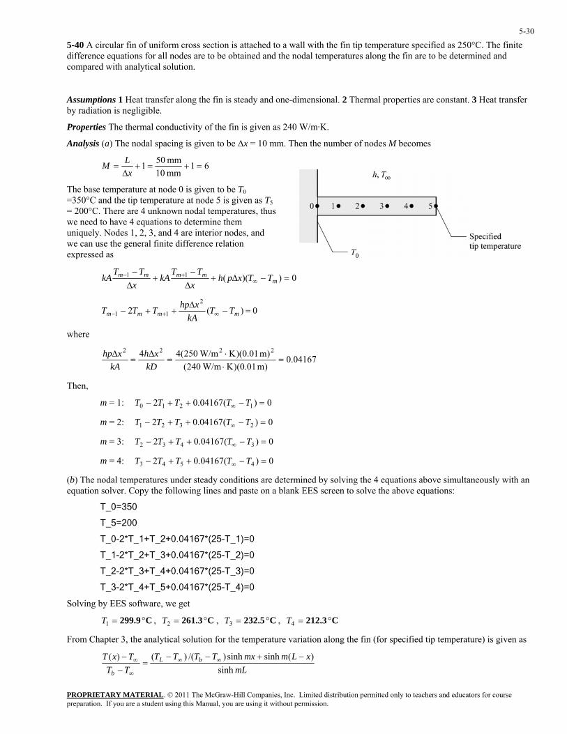
5-40 A circular fin of uniform cross section is attached to a wall with the fin tip temperature specified as 250°C. The finite difference equations for all nodes are to be obtained and the nodal temperatures along the fin are to be determined and compared with analytical solution.
Assumptions 1 Heat transfer along the fin is steady and one-dimensional. 2 Thermal properties are constant. 3 Heat transfer by radiation is negligible.
Properties The thermal conductivity of the fin is given as 240 W/m·K.
Analysis (a) The nodal spacing is given to be ∆x = 10 mm. Then the number of nodes M becomes
61mm 10mm 501 =+=+
∆=
xLM
The base temperature at node 0 is given to be T0 =350°C and the tip temperature at node 5 is given as T5 = 200°C. There are 4 unknown nodal temperatures, thus we need to have 4 equations to determine them uniquely. Nodes 1, 2, 3, and 4 are interior nodes, and we can use the general finite difference relation expressed as
0))((11 =−∆+∆−
+∆−
∞+−
mmmmm TTxph
xTT
kAx
TTkA
0)(22
11 =−∆
++− ∞+− mmmm TTkA
xhpTTT
where
04167.0)m 01.0)(K W/m240()m 01.0)(K W/m250(44 2222
=⋅⋅
=∆
=∆
kDxh
kAxhp
m = 1:
Then,
0)(04167.02 1210 =−++− ∞ TTTTT
m = 2: 0)(04167.02 2321 =−++− ∞ TTTTT
m = 3: 0)(04167.02 3432 =−++− ∞ TTTTT
m = 4: 0)(04167.02 4543 =−++− ∞ TTTTT
(b) The nodal temperatures under steady conditions are determined by solving the 4 equations above simultaneously with an llowing lines and paste on a blank EES screen to solve the above equations:
67*(25-T_3)=0
T_3-2*T_4+T + 04167*(25-T )=
, ,
equation solver. Copy the fo
T_0=350
T_5=200
T_0-2*T_1+T_2+0.04167*(25-T_1)=0
T_1-2*T_2+T_3+0.04167*(25-T_2)=0
T_2-2*T_3+T_4+0.041
_5 0. _4 0
Solving by EES software, we get
C 299.9 °=1T C 261.3 °=2T C 232.5 °=3T , C 212.3 °=4T
From Chapter 3, the analytical solution for the temperature variation along the fin (for specified tip temperature) is given as
mL
xLmmxTTTTTTTxT bL
b sinh)(sinhsinh)/()()( −+−−
=−− ∞∞
∞
∞
PROPRIETARY MATERIAL. © 2011 The McGraw-Hill Companies, Inc. Limited distribution permitted only to teachers and educators for course preparation. If you are a student using this Manual, you are using it without permission.
5-31
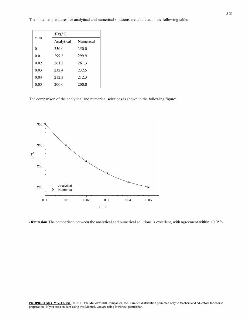
The nodal temperatures for analytical and numerical solutions are tabulated in the following table:
T(x),°C x, m
Analytical Numerical
0 350.0 350.0
0.01 299.8 299.9
0.02 261.2 261.3
0.03 232.4 232.5
0.04 212.3 212.3
0.05 200.0 200.0
The comparison of the analytical and numerical solutions is shown in the following figure:
x, m
0.00 0.01 0.02 0.03 0.04 0.05
T, °
C
200
250
300
350
AnalyticalNumerical
Discussion The comparison between the analytical and numerical solutions is excellent, with agreement within ±0.05%.
PROPRIETARY MATERIAL. © 2011 The McGraw-Hill Companies, Inc. Limited distribution permitted only to teachers and educators for course preparation. If you are a student using this Manual, you are using it without permission.
5-32
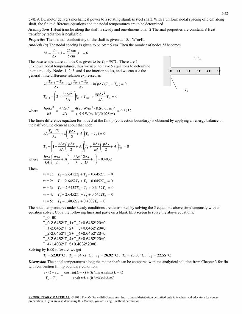
5-41 A DC motor delivers mechanical power to a rotating stainless steel shaft. With a uniform nodal spacing of 5 cm along shaft, the finite difference equations and the nodal temperatures are to be determined. Assumptions 1 Heat transfer along the shaft is steady and one-dimensional. 2 Thermal properties are constant. 3 Heat transfer by radiation is negligible. Properties The thermal conductivity of the shaft is given as 15.1 W/m·K. Analysis (a) The nodal spacing is given to be ∆x = 5 cm. Then the number of nodes M becomes
61cm 5cm 251 =+=+
∆=
xLM
The base temperature at node 0 is given to be T0 = 90°C. There are 5 unknown nodal temperatures, thus we need to have 5 equations to determine them uniquely. Nodes 1, 2, 3, and 4 are interior nodes, and we can use the general finite difference relation expressed as
0))((11 =−∆+∆−
+∆−
∞+−
mmmmm TTxph
xTT
kAx
TTkA
022
1
2
1 =∆
++⎟⎟⎠
⎞⎜⎜⎝
⎛ ∆+− ∞+− T
kAxhpTT
kAxhpT mmm
where 6452.0 W/m5.15(
)m 05.0)(K W/m25(44 2222=
⋅⋅
=∆
=∆
kDxh
kAxhp
)m 025.0)(K
he finite difference equation for node 5 at the fi tip (convection boundary) is obtained by applying an energy balance on the half volume element about that node: T n
0)(2 5
54 =−⎟⎠⎞
⎜⎝⎛ +
∆+
∆−
∞ TTAxphxTT
kA
022
1 54 =⎟⎠⎞
⎜⎝⎛ +
∆∆+⎥
⎦
⎤⎢⎣
⎡⎟⎠⎞
⎜⎝⎛ +
∆∆+− ∞TAxp
kAxhTAxp
kAxhT
4032.0122
=⎟⎠⎞
⎜⎝⎛ +
∆∆=⎟
⎠⎞
⎜⎝kA
⎛ +∆ pxhwhere ∆
Dx
kxhAx
hen, T m = 1: 06452.06452.2 210 =++− ∞TTTT
m = 2: − 06452.06452.2 321 =++ ∞TTTT
m = 3: 06452.06452.2 432 =++− ∞TTTT
m = 4: 06452.06452.23 54 =++− TTTT ∞
m = 5: 04032.04032.1 54 =+− ∞TTT The nodal temperatures under steady conditions are determined by solving the 5 equations above simultaneously with an
lank EES screen to solve the above equations:
0.6452*20=0 T_2-2.6452* 3 _4+0.6452*2 0
1T , ,
equation solver. Copy the following lines and paste on a b T_0=90 T_0-2.6452*T_1+T_2+0.6452*20=0 T_1-2.6452*T_2+T_3+ T_ +T 0= T_3-2.6452*T_4+T_5+0.6452*20=0 T_4-1.4032*T_5+0.4032*20=0
ving by EES software, we get Sol = C 52.03 ° C 34.72 °=2T C 26.92 °=3T , C 23.58 °=4T , C 22.55 °=5T
Discussion The nodal temperatures along the motor shaft can be compared with the analytical solution from Chapter 3 for fin with convection fin tip boundary condition:
mLmkhmL
xLmmkhxLmTTTxT
b sinh)/(cosh)(sinh)/()(cosh)(
+−+−
=−−
∞
∞
PROPRIETARY MATERIAL. © 2011 The McGraw-Hill Companies, Inc. Limited distribution permitted only to teachers and educators for course preparation. If you are a student using this Manual, you are using it without permission.
5-33
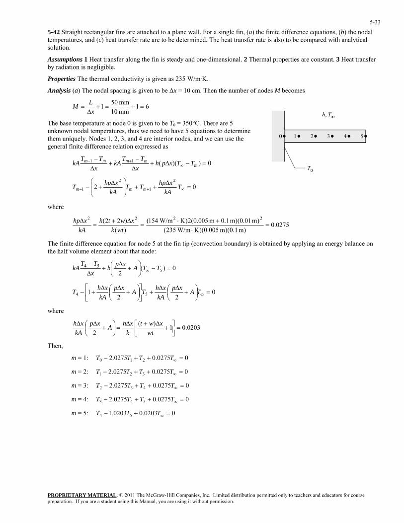
5-42 Straight rectangular fins are attached to a plane wall. For a single fin, (a) the finite difference equations, (b) the nodal temperatures, and (c) heat transfer rate are to be determined. The heat transfer rate is also to be compared with analytical solution.
Assumptions 1 Heat transfer along the fin is steady and one-dimensional. 2 Thermal properties are constant. 3 Heat transfer by radiation is negligible.
Properties The thermal conductivity is given as 235 W/m·K.
Analysis (a) The nodal spacing is given to be ∆x = 10 cm. Then the number of nodes M becomes
61mm 01mm 051 =+=+
∆=
xLM
The base temperature at node 0 is given to be T0 = 350°C. There are 5 unknown nodal temperatures, thus we need to have 5 equations to determine them uniquely. Nodes 1, 2, 3, and 4 are interior nodes, and we can use the general finite difference relation expressed as
0))((11 =−∆+∆−
+∆−
∞+−
mmmmm TTxph
xTT
kAx
TTkA
022
1
2
1 =∆
++⎟⎟⎠
⎞⎜⎜⎝
⎛ ∆+− ∞+− T
kAxhpTT
kAxhpT mmm
where
0275.0)m 01.0)(m 1.0m 005.0(2)K W/m154()()22( 2222
=+⋅
=∆+
=∆
wtkxwth
kAxhp
)m 1.0)(m 005.0)(K W/m235( ⋅
he finite difference equation for node 5 at the fi tip (convection boundary) is obtained by applying an energy balance on e half volume element about that node:
T nth
0)(2 5
54 =−⎟⎠⎞
⎜⎝⎛ +
∆+
∆−
∞ TTAxphxTT
kA
022
1 54 =⎟⎠⎞
⎜⎝⎛ +
∆∆+⎥
⎦
⎤⎢⎣
⎡⎟⎠⎞
⎜⎝⎛ +
∆∆+− ∞TAxp
kAxhTAxp
kAxhT
where
0203.01)(2
=⎥⎦⎤
⎢⎣⎡ +
∆+∆=⎟
⎠⎞
⎜⎛ +
∆ pkA
xh ⎝
∆wt
xwtk
xhAx
Then,
m = 1: 00275.00275.2 210 =++− ∞TTTT
m = 2: 00275.00275.2 321 =++− ∞TTTT
m = 3: 00275.00275.2 432 =++− ∞TTTT
m = 4: 00275.00275.2 543 =++− ∞TTTT
m = 5: 00203.00203.1 54 =+− ∞TTT
PROPRIETARY MATERIAL. © 2011 The McGraw-Hill Companies, Inc. Limited distribution permitted only to teachers and educators for course preparation. If you are a student using this Manual, you are using it without permission.
5-34
T ,
(b) The nodal temperatures under steady conditions are determined by solving the 5 equations above simultaneously with an equation solver. Copy the following lines and paste on a blank EES screen to solve the above equations:
T_0=350
T_0-2.0275*T_1+T_2+0.0275*25=0
T_1-2.0275*T_2+T_3+0.0275*25=0
T_2-2.0275*T_3+T_4+0.0275*25=0
T_3-2.0275*T_4+T_5+0.0275*25=0
T_4-1.0203*T_5+0.0203*25=0
Solving by EES software, we get
, =2C 316.6 °=1T C 291.2 ° C 273.2 °=3T , C 261.9 °=4T , C 257.2 °=5T
(c) The rate of heat transfer from a single fin is simply the sum of the heat transfer from the nodal elements,
W445=
−⎟⎠⎞
⎜⎝⎛ +
∆+−+++∆+−
∆=
−==
∞∞∞
=∞
= 0 surface,
0 element,num ,fin
mmm
mm
∑∑
)(2
)4()(2
)(
543210
55
TTAxphTTTTTxhpTTxhp
TThAQQ &&
or straight angular fins, the analytical solution from Chapter 3 for the heat transfer rate is,
ThAQ bη&
here
F rect
W427=°−⋅=−= ∞ C )25350)(m 0105.0)(K W/m154)(813.0()( 22finfinexact fin, T
w
1m 19.162 -
kthm ==
m 0525.02/ =+= tLLc
2fin m 0105.02 == cwLA
8130tanh
fin .mL
mL
c
c ==η
Discussion The comparison between the analytical and numerical solutions is within ±4.3% agreement. One way to increase the accuracy of the numerical solution is by reducing the nodal spacing, thereby increasing the number of nodes.
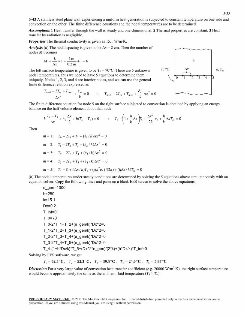
PROPRIETARY MATERIAL. © 2011 The McGraw-Hill Companies, Inc. Limited distribution permitted only to teachers and educators for course preparation. If you are a student using this Manual, you are using it without permission.
5-35
5-43 A stainless steel plane wall experiencing a uniform heat generation is subjected to constant temperature on one side and convection on the other. The finite difference equations and the nodal temperatures are to be determined. Assumptions 1 Heat transfer through the wall is steady and one-dimensional. 2 Thermal properties are constant. 3 Heat transfer by radiation is negligible. Properties The thermal conductivity is given as 15.1 W/m·K. Analysis (a) The nodal spacing is given to be ∆x = 2 cm. Then the number of nodes M becomes
61m 2.0∆
m 11 =+=+=x
LM
n
or nodes, and we can use the general finite difference relation expressed as
The left surface temperature is given to be T0 = 70°C. There are 5 unknownodal temperatures, thus we need to have 5 equations to determine them uniquely. Nodes 1, 2, 3, and 4 are interi
02
2∆ kx11 =+
+− +− eTTT mmmm & → 02 2
11 =∆++− +− xk
The finite difference equation for node 5 on the right
eTTT m
mmm&
surface subjected to convection is obtained by applying an energy balance on the half volume element about that node:
0)(2 55
54 =−+∆
+∆−
∞ TThxexTT
k & → 02
1 5
2
54 =∆+∆
+⎟⎠⎞
⎜⎝⎛ ∆+− ∞xT
khe
kxTx
khT &
Then
=∆++− xkeTTT &
=∆++− xkeTTT &
r steady conditions are determined by solving the 5 equations above simultaneously with an ng lines and paste on a blank EES screen to solve the above equations:
x^2*e_gen)/(2*k)+(h*Dx/k)*T_inf=0
olving by S software, ge
m2·K), the right surface temperature would become approximately the same as the ambient fluid temperature (T5 ≈ T∞).
0)/(2 2121 m = 1: 0
m = 2: 0)/(2 22321 =∆++− xkeTTT &
0)/(2 2343 m = 3: 2
0)/(2 24543 =∆++− xkeTTT & m = 4:
m = 5: 0)/()2/()()/1( 52
54 =∆+∆+∆+− ∞TkxhkexTkxhT &
(b) The nodal temperatures undeequation solver. Copy the followi e_gen=1000
h=250
k=15.1
Dx=0.2
T_inf=0
T_0=70
T_0-2*T_1+T_2+(e_gen/k)*Dx^2=0
T_1-2*T_2+T_3+(e_gen/k)*Dx^2=0
T_2-2*T_3+T_4+(e_gen/k)*Dx^2=0
T_3-2*T_4+T_5+(e_gen/k)*Dx^2=0
T_4-(1+h*Dx/k)*T_5+(D
S EE we t C 62.5 °=1T , C 52.3 °=2T , C 39.5 °=3T , C 24.0 °=4T , C 5.87 °=5T
Discussion For a very large value of convection heat transfer coefficient (e.g. 20000 W/
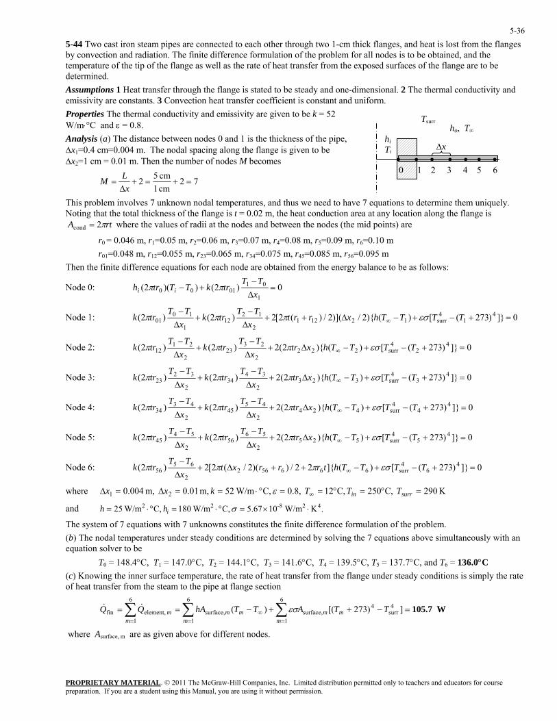
PROPRIETARY MATERIAL. © 2011 The McGraw-Hill Companies, Inc. Limited distribution permitted only to teachers and educators for course preparation. If you are a student using this Manual, you are using it without permission.
5-36
5-44 Two cast iron steam pipes are connected to each other through two 1-cm thick flanges, and heat is lost from the flanges by convection and radiation. The finite difference formulation of the problem for all nodes is to be obtained, and the temperature of the tip of the flange as well as the rate of heat transfer from the exposed surfaces of the flange are to be determined. Assumptions 1 Heat transfer through the flange is stated to be steady and one-dimensional. 2 The thermal conductivity and emissivity are constants. 3 Convection heat transfer coefficient is constant and uniform. Properties The thermal conductivity and emissivity are given to be k = 52 W/m⋅°C and ε = 0.8.
hi Ti
∆x• • • • • • •
0 1 2 3 4 5 6
ho, T∞
Tsurr
Analysis (a) The distance between nodes 0 and 1 is the thickness of the pipe, ∆x1=0.4 cm=0.004 m. The nodal spacing along the flange is given to be ∆x2=1 cm = 0.01 m. Then the number of nodes M becomes
72cm 1cm 52 =+=+
∆=
xLM
This problem involves 7 unknown nodal temperatures, and thus we need to have 7 equations to determine them uniquely. Noting that the total thickness of the flange is t = 0.02 m, the heat conduction area at any location along the flange is
rtA π2cond = where the values of radii at the nodes and between the nodes (the mid points) are
r0 = 0.046 m, r1=0.05 m, r2=0.06 m, r3=0.07 m, r4=0.08 m, r5=0.09 m, r6=0.10 m r01=0.048 m, r12=0.055 m, r23=0.065 m, r34=0.075 m, r45=0.085 m, r56=0.095 m Then the finite difference equations for each node are obtained from the energy balance to be as follows:
Node 0: 0)2())(2(1
010100 =
∆−
+−xTT
trkTTtrh ii ππ
Node 1: 0]})273([)(){2/)](2/)(2[2)2()2( 41
4surr12121
2
1212
1
1001 =+−+−∆++
∆−
+∆−
∞ TTTThxrrtx
TTtrk
xTT
trk εσπππ
Node 2: 0]})273([)(){2(2)2()2( 42
4surr222
2
2323
2
2112 =+−+−∆+
∆−
+∆−
∞ TTTThxtrx
TTtrk
xTT
trk εσπππ
0]})273([)(){2(2)2()2( 43
4surr323
2
3434
2
3223 =+−+−∆+
∆−
+∆−
∞ TTTThxtrx
TTtrk
xTT
trk εσπππNode 3:
Node 4: 0]})273([)(){2(2)2()2( 44
4surr424
2
4545
2
4334 =+−+−∆+
∆−
+∆−
∞ TTTThxtrx
TTtrk
xTT
trk εσπππ
Node 5: 0]})273([)(){2(2)2()2( 45
4surr525
2
5656
2
5445 =+−+−∆+
∆−
+∆−
∞ TTTThxtrx
TTtrk
xTT
trk εσπππ
Node 6: 0]})273([)(]{t22/))(2/(2[2)2( 46
4surr666562
6556 =+−+−++∆+
−∞ TTTThrrrxt
TTtrk εσπππ
2∆x
where K 290 ,C250 C,12 0.8, C, W/m52 m, 01.0 m, 004.0 21 =°=°==°⋅==∆=∆ ∞ surrin TTTkxx ε
and W/m25 2=h .C, ×i K W/m105.67 C, W/m180 42-82 ⋅=°⋅=°⋅ σh
0 14 °C, T4 = 139.5°C, T5 = 137.7°C, and T6 = 136.0°C transfer from the flange under steady conditions is simply the rate
of heat transfer from the steam to the pipe at flange section
where Asurface, m are as given above for different nodes.
The system of 7 equations with 7 unknowns constitutes the finite difference formulation of the problem. (b) The nodal temperatures under steady conditions are determined by solving the 7 equations above simultaneously with an equation solver to be T 8.4°C, T = 1 = 147.0°C, T2 = 144.1°C, T3 = 141.6(c) Knowing the inner surface temperature, the rate of heat
W105.7=−++−== ∑∑∑==
∞=
])273[()( 4surr
46
1surface,
6
1surface,
6
1 element,fin TTATThAQQ m
mm
mmm
mm εσ&&
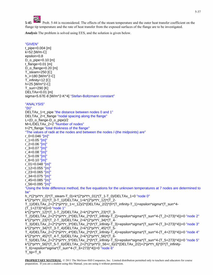
PROPRIETARY MATERIAL. © 2011 The McGraw-Hill Companies, Inc. Limited distribution permitted only to teachers and educators for course preparation. If you are a student using this Manual, you are using it without permission.
5-37
5-45 Prob. 5-44 is reconsidered. The effects of the steam temperature and the outer heat transfer coefficient on the flange tip temperature and the rate of heat transfer from the exposed surfaces of the flange are to be investigated.
Analysis The problem is solved using EES, and the solution is given below.
"GIVEN" t_pipe=0.004 [m] k=52 [W/m-C] epsilon=0.8 D_o_pipe=0.10 [m] t_flange=0.01 [m] D_o_flange=0.20 [m] T_steam=250 [C] h_i=180 [W/m^2-C] T_infinity=12 [C] h=25 [W/m^2-C] T_surr=290 [K] DELTAx=0.01 [m] sigma=5.67E-8 [W/m^2-K^4] “Stefan-Boltzmann constant" "ANALYSIS" "(b)" DELTAx_1=t_pipe "the distance between nodes 0 and 1" DELTAx_2=t_flange "nodal spacing along the flange" L=(D_o_flange-D_o_pipe)/2 M=L/DELTAx_2+2 "Number of nodes" t=2*t_flange "total thixkness of the flange" "The values of radii at the nodes and between the nodes /-(the midpoints) are" r_0=0.046 "[m]" r_1=0.05 "[m]" r_2=0.06 "[m]" r_3=0.07 "[m]" r_4=0.08 "[m]" r_5=0.09 "[m]" r_6=0.10 "[m]" r_01=0.048 "[m]" r_12=0.055 "[m]" r_23=0.065 "[m]" r_34=0.075 "[m]" r_45=0.085 "[m]" r_56=0.095 "[m]" "Using the finite difference method, the five equations for the unknown temperatures at 7 nodes are determined to be" h_i*(2*pi*t*r_0)*(T_steam-T_0)+k*(2*pi*t*r_01)*(T_1-T_0)/DELTAx_1=0 "node 0" k*(2*pi*t*r_01)*(T_0-T_1)/DELTAx_1+k*(2*pi*t*r_12)*(T_2-T_1)/DELTAx_2+2*2*pi*t*(r_1+r_12)/2*(DELTAx_2/2)*(h*(T_infinity-T_1)+epsilon*sigma*(T_surr^4-(T_1+273)^4))=0 "node 1" k*(2*pi*t*r_12)*(T_1-T_2)/DELTAx_2+k*(2*pi*t*r_23)*(T_3-T_2)/DELTAx_2+2*2*pi*t*r_2*DELTAx_2*(h*(T_infinity-T_2)+epsilon*sigma*(T_surr^4-(T_2+273)^4))=0 "node 2" k*(2*pi*t*r_23)*(T_2-T_3)/DELTAx_2+k*(2*pi*t*r_34)*(T_4-T_3)/DELTAx_2+2*2*pi*t*r_3*DELTAx_2*(h*(T_infinity-T_3)+epsilon*sigma*(T_surr^4-(T_3+273)^4))=0 "node 3" k*(2*pi*t*r_34)*(T_3-T_4)/DELTAx_2+k*(2*pi*t*r_45)*(T_5-T_4)/DELTAx_2+2*2*pi*t*r_4*DELTAx_2*(h*(T_infinity-T_4)+epsilon*sigma*(T_surr^4-(T_4+273)^4))=0 "node 4" k*(2*pi*t*r_45)*(T_4-T_5)/DELTAx_2+k*(2*pi*t*r_56)*(T_6-T_5)/DELTAx_2+2*2*pi*t*r_5*DELTAx_2*(h*(T_infinity-T_5)+epsilon*sigma*(T_surr^4-(T_5+273)^4))=0 "node 5" k*(2*pi*t*r_56)*(T_5-T_6)/DELTAx_2+2*(2*pi*t*(r_56+r_6)/2*(DELTAx_2/2)+2*pi*t*r_6)*(h*(T_infinity-T_6)+epsilon*sigma*(T_surr^4-(T_6+273)^4))=0 "node 6" T_tip=T_6
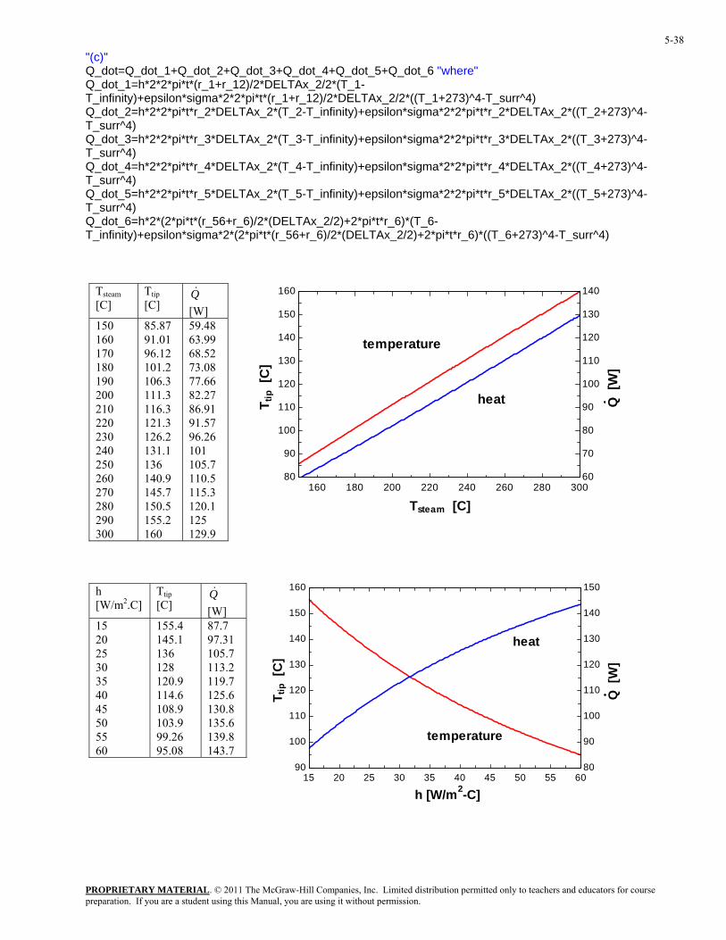
PROPRIETARY MATERIAL. © 2011 The McGraw-Hill Companies, Inc. Limited distribution permitted only to teachers and educators for course preparation. If you are a student using this Manual, you are using it without permission.
5-38
"(c)" Q_dot=Q_dot_1+Q_dot_2+Q_dot_3+Q_dot_4+Q_dot_5+Q_dot_6 "where" Q_dot_1=h*2*2*pi*t*(r_1+r_12)/2*DELTAx_2/2*(T_1-T_infinity)+epsilon*sigma*2*2*pi*t*(r_1+r_12)/2*DELTAx_2/2*((T_1+273)^4-T_surr^4) Q_dot_2=h*2*2*pi*t*r_2*DELTAx_2*(T_2-T_infinity)+epsilon*sigma*2*2*pi*t*r_2*DELTAx_2*((T_2+273)^4-T_surr^4) Q_dot_3=h*2*2*pi*t*r_3*DELTAx_2*(T_3-T_infinity)+epsilon*sigma*2*2*pi*t*r_3*DELTAx_2*((T_3+273)^4-T_surr^4) Q_dot_4=h*2*2*pi*t*r_4*DELTAx_2*(T_4-T_infinity)+epsilon*sigma*2*2*pi*t*r_4*DELTAx_2*((T_4+273)^4-T_surr^4) Q_dot_5=h*2*2*pi*t*r_5*DELTAx_2*(T_5-T_infinity)+epsilon*sigma*2*2*pi*t*r_5*DELTAx_2*((T_5+273)^4-T_surr^4) Q_dot_6=h*2*(2*pi*t*(r_56+r_6)/2*(DELTAx_2/2)+2*pi*t*r_6)*(T_6-T_infinity)+epsilon*sigma*2*(2*pi*t*(r_56+r_6)/2*(DELTAx_2/2)+2*pi*t*r_6)*((T_6+273)^4-T_surr^4)
Tsteam [C]
Ttip [C]
Q& [W]
150 160 170 180 190 200 210 220 230 240 250 260 270 280 290 300
85.87 91.01 96.12 101.2 106.3 111.3 116.3 121.3 126.2 131.1 136 140.9 145.7 150.5 155.2 160
59.48 63.99 68.52 73.08 77.66 82.27 86.91 91.57 96.26 101 105.7 110.5 115.3 120.1 125 129.9
160 180 200 220 240 260 280 30080
90
100
110
120
130
140
150
160
60
70
80
90
100
110
120
130
140
Tsteam [C]
T tip
[C
]
Q [
W]
temperature
heat
h [W/m2.C]
T tip[C]
Q& [W]
15 20 25 30 35 40 45 50 55 60
155.4 145.1 136 128 120.9 114.6 108.9 103.9 99.26 95.08
87.7 97.31 105.7 113.2 119.7 125.6 130.8 135.6 139.8 143.7
15 20 25 30 35 40 45 50 55 6090
100
110
120
130
140
150
160
80
90
100
110
120
130
140
150
h [W/m2-C]
T tip
[C
]
Q [
W]
temperature
heat
PROPRIETARY MATERIAL. © 2011 The McGraw-Hill Companies, Inc. Limited distribution permitted only to teachers and educators for course preparation. If you are a student using this Manual, you are using it without permission.
5-39
5-46 Using EES, the solutions of the systems of algebraic equations are determined to be as follows:
olution: x1 = 2, x2 = 3, x3 = −1
2
11.964
olution: x1 = 2.33, x2 = 2.29, x3 = −1.62
"(a)"
3*x_1-x_2+3*x_3=0
-x_1+2*x_2+x_3=3
2*x_1-x_2-x_3=2
S
"(b)"
4*x_1-2*x_2^2+0.5*x_3=-
x_1^3-x_2+-x_3=
x_1+x_2+x_3=3
S
5-47 Using EES, the solutions of the systems of algebraic equations are determined to be as follows:
_4=6
4=2
olution: x1 = 13, x2 = −9, x3 = 13, x4 = −2
93
olution: x1 = 2.825, x2 = 1.791, x3 = −1.841
"(a)"
3*x_1+2*x_2-x_3+x
x_1+2*x_2-x_4=-3
-2*x_1+x_2+3*x_3+x_
3*x_2+x_3-4*x_4=-6
S
"(b)"
3*x_1+x_2^2+2*x_3=8
-x_1^2+3*x_2+2*x_3=-6.2
2*x_1-x_2^4+4*x_3=-12
S
PROPRIETARY MATERIAL. © 2011 The McGraw-Hill Companies, Inc. Limited distribution permitted only to teachers and educators for course preparation. If you are a student using this Manual, you are using it without permission.
5-40
5-48 Using EES, the solutions of the systems of algebraic equations are determined to be as follows:
=-1
olution: x1 = −2, x2 = −1, x3 = 0, x4 = 1
*x_4=-3
Solution: x1 = 0.263, x2 = −1.15, x3 = 1.70, x4 = 2.14
"(a)"
4*x_1-x_2+2*x_3+x_4=-6
x_1+3*x_2-x_3+4*x_4
-x_1+2*x_2+5*x_4=5
2*x_2-4*x_3-3*x_4=-5
S
"(b)"
2*x_1+x_2^4-2*x_3+x_4=1
x_1^2+4*x_2+2*x_3^2-2
-x_1+x_2^4+5*x_3=10
3*x_1-x_3^2+8*x_4=15
PROPRIETARY MATERIAL. © 2011 The McGraw-Hill Companies, Inc. Limited distribution permitted only to teachers and educators for course preparation. If you are a student using this Manual, you are using it without permission.
5-41
Two-Dimensional Steady Heat Conduction
5-49C A region that cannot be filled with simple volume elements such as strips for a plane wall, and rectangular elements for two-dimensional conduction is said to have irregular boundaries. A practical way of dealing with such geometries in the finite difference method is to replace the elements bordering the irregular geometry by a series of simple volume elements.
5-50C For a medium in which the finite difference formulation of a general interior node is given in its simplest form as : 4/)( bottomrighttopleftnode TTTTT +++=
(a) Heat transfer is steady, (b) heat transfer is two-dimensional, (c) there is no heat generation in the medium, (d) the nodal spacing is constant, and (e) the thermal conductivity of the medium is constant.
5-51C For a medium in which the finite difference formulation of a general interior node is given in its simplest form as
042
nodenodebottomrighttopleft k
(a) Heat transfer is steady, (b) heat transfer is two-dimensional, (c) there is heat generat
=+−+++le
TTTTT&
:
ion in the medium, (d) the nodal acing is constant, and (e) the thermal conductivity of the medium is constant.
sp
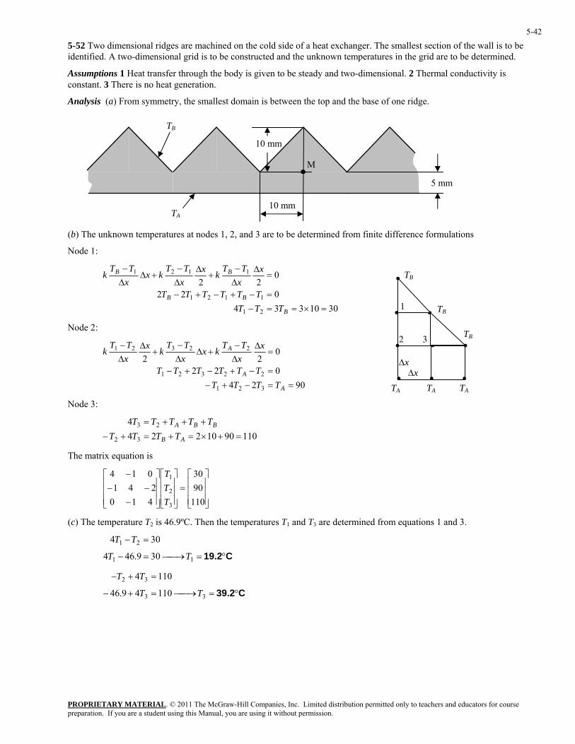
PROPRIETARY MATERIAL. © 2011 The McGraw-Hill Companies, Inc. Limited distribution permitted only to teachers and educators for course preparation. If you are a student using this Manual, you are using it without permission.
5-42
5-52 Two dimensional ridges are machined on the cold side of a heat exchanger. The smallest section of the wall is to be identified. A two-dimensional grid is to be constructed and the unknown temperatures in the grid are to be determined.
Assumptions 1 Heat transfer through the body is given to be steady and two-dimensional. 2 Thermal conductivity is constant. 3 There is no heat generation.
Analysis (a) From symmetry, the smallest domain is between the top and the base of one ridge.
5 mm
10 mm TA
TB
M
10 mm
(b) The unknown temperatures at nodes 1, 2, and 3 are to be determined from finite difference formulations
Node 1:
3010334022
022
21
1121
1121
=×==−=−+−+−
=∆
∆−
+∆
∆−
+∆∆−
B
BB
BB
TTTTTTTTT
xxTT
kxxTT
kxxTT
k
Node 2:
9024022
022
3T21
22321
22321
==−+−=−+−+−
=∆
∆−
+∆∆−
+∆
∆−
A
A
A
TTTTTTTTT
xxTT
kxxTT
kxxT
k
Node 3:
32
23
=+×=+=+−+++
AB
BBA
TTTTTT
241014
3
2
1
TTT
(c) The temperature T2 is 46.9ºC. Then the temperatures T1 and T3 are determined from equations 1 and 3.
• •
• • •
• • •
∆x
1
•
2 3
TA TA TA
TB
TB
TB
∆x
T
4 = TTT 1109010224
The matrix equation is
⎥⎥⎥
⎦
⎤
⎢⎢⎢
⎣
⎡=
⎥⎥⎥
⎦
⎤
⎢⎢⎢
⎣
⎡
⎥⎥⎥
⎦
⎤
⎢⎢⎢
⎣
⎡
−−−
−
1109030
410
C19.2°=⎯→⎯=−
=−
11
21
309.464
304
TT
TT
C39.2°=⎯→⎯=+−
=+−
33
32
11049.46
1104
TT
TT
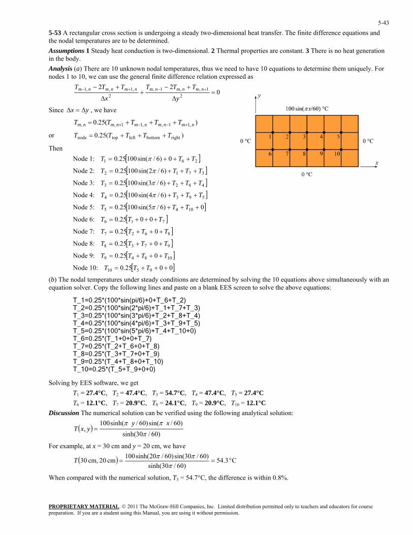
PROPRIETARY MATERIAL. © 2011 The McGraw-Hill Companies, Inc. Limited distribution permitted only to teachers and educators for course preparation. If you are a student using this Manual, you are using it without permission.
5-43
5-53 A rectangular cross section is undergoing a steady two-dimensional heat transfer. The finite difference equations and the nodal temperatures are to be determined. Assumptions 1 Steady heat conduction is two-dimensional. 2 Thermal properties are constant. 3 There is no heat generation in the body. Analysis (a) There are 10 unknown nodal temperatures, thus we need to have 10 equations to determine them uniquely. For nodes 1 to 10, we can use the general finite difference relation expressed as
022
21 , ,1 ,
2 ,1 , ,1 =
∆
+−+
∆
+− +−+−
y
TTT
x
TTT nmnmnmnmnmnm
Since yx ∆= , we∆ have
)(25.0 ,11 , ,11 , , nmnmnmnmnm TTTTT +−−+ +++=
or )(25.0 rightbottomlefttopnode TTTTT +++=
Then Node 1: [ ]261 0)6/sin(10025.0 TTT +++= π
Node 2: [ ]3712 )6/2sin(10025.0 TTTT +++= π
Node 3: [ ]4823 )6/3sin(10025.0 TTTT +++= π
Node 4: [ ]5934 )6/4sin(10025.0 TTTT +++= π
Node 5: [ ]0)6/5sin(10025.0 1045 +++= TTT π
Node 6: [ ]716 0025.0 TTT +++=
Node 7: T [ ]8627 025.0 TTT +++=
+++=
Node 8: [ ]9738 025.0 TTTT +++=
Node 9: [ ]10849 025.0 TTTT +++=
Node 10: [ ]0025.0 9510 TTT
(b) The nodal temperatures under steady conditions are determined by solving the 10 equations above simultaneously with an ion solver. Copy the following lines and paste on a blank EES screen to solve the above equations: equat
T_1=0.25*(100*sin(pi/6)+0+T_6+T_2) T_2=0.25*(100*sin(2*pi/6)+T_1+T_7+T_3) T_3=0.25*(100*sin(3*pi/6)+T_2+T_8+T_4) T_4=0.25*(100*sin(4*pi/6)+T_3+T_9+T_5)
10+0) T_5=0.25*(100*sin(5*pi/6)+T_4+T_ T_6=0.25*(T_1+0+0+T_7) T_7=0.25*(T_2+T_6+0+T_8) T_8=0.25*(T_3+T_7+0+T_9) T_9=0.25*(T_4+T_8+0+T_10) T_10=0.25*(T_5+T_9+0+0)
olving S by EES software, we get T1 = 27.4°C, T2 = 47.4°C, T3 = 54.7°C, T4 = 47.4°C, T5 = 27.4°C T6 = 12.1°C, T7 = 20.9°C, T8 = 24.1°C, T9 = 20.9°C, T10 = 12.1°C Discussion The numerical solution can be verified using the following analytical solution:
( ))60/30sinh(
)60/sin()60/sinh(100,
πππ xy
yxT =
For example, at x = 30 cm and y = 20 cm, we have
( ) C 3.54)60/30sinh(
)60/30sin()60/20sinh(100cm 20 ,cm 30 °==π
ππT
When compared with the numerical solution, T3 = 54.7°C, the difference is within 0.8%.
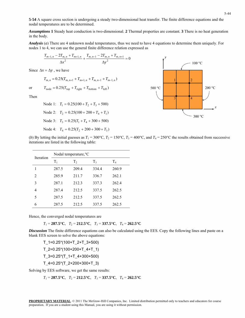
PROPRIETARY MATERIAL. © 2011 The McGraw-Hill Companies, Inc. Limited distribution permitted only to teachers and educators for course preparation. If you are a student using this Manual, you are using it without permission.
5-44
5-54 A square cross section is undergoing a steady two-dimensional heat transfer. The finite difference equations and the nodal temperatures are to be determined.
Assumptions 1 Steady heat conduction is two-dimensional. 2 Thermal properties are constant. 3 There is no heat generation in the body.
Analysis (a) There are 4 unknown nodal temperatures, thus we need to have 4 equations to determine them uniquely. For nodes 1 to 4, we can use the general finite difference relation expressed as
022
21 , ,1 ,
2 ,1 , ,1 =
∆
+−+
∆
+− +−+−
y
TTT
x
TTT nmnmnmnmnmnm
Since yx ∆= , we∆ have
)(25.0 ,11 , ,11 , , nmnmnmnmnm TTTTT −−++ +++=
or )(25.0 leftbottomrighttopnode TTTTT +++=
Then
Node 1: )500100(25.0 321 +++= TTT
Node 2: )200100(25.0 142 TTT +++=
Node 3: )500300(25.0 413 +++= TTT
Node 4: )300200(25.0 324 TTT +++=
(b) By letting the initial guesses as T1 = 300°C, T2 = 150°C, T3 = 400°C, and T4 = 250°C the results obtained from successive iterations are listed in the following table:
Nodal temperature,°C Iteration
T1 T2 T3 T4
1 287.5 209.4 334.4 260.9
2 285.9 211.7 336.7 262.1
3 287.1 212.3 337.3 262.4
4 287.4 212.5 337.5 262.5
5 287.5 212.5 337.5 262.5
6 287.5 212.5 337.5 262.5
Hence, the converged nodal temperatures are
T1 = 287.5°C, T2 = 212.5°C, T3 = 337.5°C, T4 = 262.5°C
Discussion The finite difference equations can also be calculated using the EES. Copy the following lines and paste on a blank EES screen to solve the above equations:
T_1=0.25*(100+T_2+T_3+500)
T_2=0.25*(100+200+T_4+T_1)
T_3=0.25*(T_1+T_4+300+500)
T_4=0.25*(T_2+200+300+T_3)
Solving by EES software, we get the same results:
T1 = 287.5°C, T2 = 212.5°C, T3 = 337.5°C, T4 = 262.5°C
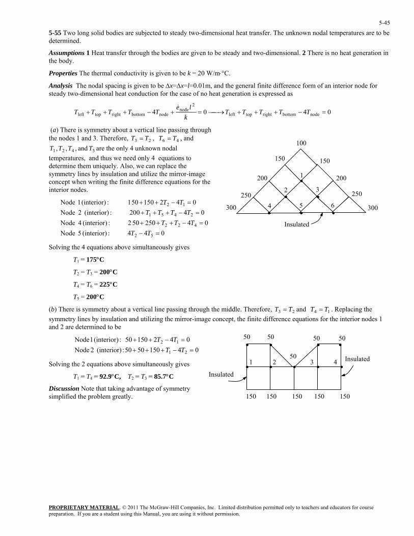
PROPRIETARY MATERIAL. © 2011 The McGraw-Hill Companies, Inc. Limited distribution permitted only to teachers and educators for course preparation. If you are a student using this Manual, you are using it without permission.
5-45
5-55 Two long solid bodies are subjected to steady two-dimensional heat transfer. The unknown nodal temperatures are to be determined.
Assumptions 1 Heat transfer through the bodies are given to be steady and two-dimensional. 2 There is no heat generation in the body.
Properties The thermal conductivity is given to be k = 20 W/m⋅°C.
Analysis The nodal spacing is given to be ∆x=∆x=l=0.01m, and the general finite difference form of an interior node for steady two-dimensional heat conduction for the case of no heat generation is expressed as
0404 nodebottomrighttopleft
2node
nodebottomrighttopleft =−+++⎯→⎯=+−+++ TTTTTk
leTTTTT
&
(a) There is symmetry about a vertical line passing through the nodes 1 and 3. Therefore, = 46 T= and
5421 and ,,, TTTT are the only 4 unknown nodal temperatures, and thus we need only 4 equations to determine them uniquely. Also, we can replace the symmetry lines by insulation and utilize the mirror-imageconcept when writing the finite d
23 TT , ,
ifference equations for the
interior nodes.
422
2451
12
=−+++=−+++
=−++
TTTTTTT
TT
olving t s above simultaneously gives
°C
T100
Insulated
•
• •
• • •
1
2 3
4 5 6
150
200
250
300
150
200
250
300
0402550 2 :(interior) 4 Node04200 :(interior) 2 Node
04201550 1 :(interior) 1 Node
044 :(interior) 5 Node 52 =− TT
S he 4 equation
T1 = 175°C
T2 = T3 = 200°C
T4 = T6 = 225
T5 = 200°C
(b) There is symmetry about a vertical line passing through the middle. Therefore, 23 TT = and 14 TT = . Replacing the symmetry lines by insulation and utilizing the mirror-image concept, the finite difference equations for the interior nodes 1 and 2 are determined to be
2
T3 = 85.7°C
iscussion Note that taking advantage of symmetry mplified the problem greatly.
• • • • 50 50
31 2 4• • • • •
Insulated
50 50
150 150 150 150 150
Insulated 5040150550 :(interior) 2 Node
04201550 :(interior) 1 Node 12
=−+++=−++TT
TT01
Solving the 2 equations above simultaneously gives
T1 = T4 = 92.9°C, T2 =
Dsi
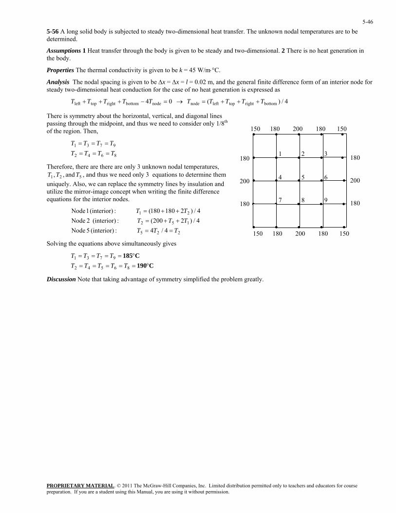
PROPRIETARY MATERIAL. © 2011 The McGraw-Hill Companies, Inc. Limited distribution permitted only to teachers and educators for course preparation. If you are a student using this Manual, you are using it without permission.
5-46
5-56 A long solid body is subjected to steady two-dimensional heat transfer. The unknown nodal temperatures are to be determined.
Assumptions 1 Heat transfer through the body is given to be steady and two-dimensional. 2 There is no heat generation in the body.
Properties The thermal conductivity is given to be k = 45 W/m⋅°C.
Analysis The nodal spacing is given to be ∆x = ∆x = l = 0.02 m, and the general finite difference form of an interior node for steady two-dimensional heat conduction for the case of no heat generation is expressed as
4/)( 04 bottomrighttopleftnodenodebottomrighttopleft TTTTTTTTTT +++=→=−+++
There is symmetry about the horizontal, vertical, and diagonal lines passing through the midpoint, and thus we need to consider only 1/8th of the region. Then,
8642 TTTT ===
Therefore, there are there are only 3 unknown nodal temperatures, 521 and , , TTT , and thus we need only 3 equations to determine them
uniquely. Also, we can replace the symmetry lines by insulation andutilize the mirror-image concept w
9731 TTTT ===
hen writing the finite difference
equations for the interior nodes.
4/4 :(interior) 5 Node4/)2200( :(interior) 2 Node4/)
TTTTTT
==++=
225
152
21 2180180( :(interior) 1 Node T
T
++=
Discussion Note that taking advantage of symmetry simplified the problem greatly.
• • • • •
• • • • •
180 200 180
• • • • •
• • • • •
• • • • •
150 180 200 180 150
150 180 200 180 150
180 200 180
1 2 3
4 5 6
7 8 9
Solving the equations above simultaneously gives
C190C185
°=====°====
86542
9731
TTTTTTTTT
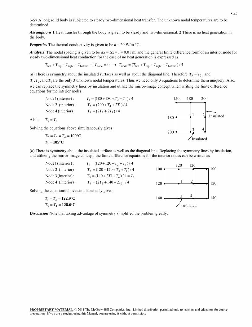
PROPRIETARY MATERIAL. © 2011 The McGraw-Hill Companies, Inc. Limited distribution permitted only to teachers and educators for course preparation. If you are a student using this Manual, you are using it without permission.
5-47
5-57 A long solid body is subjected to steady two-dimensional heat transfer. The unknown nodal temperatures are to be determined.
Assumptions 1 Heat transfer through the body is given to be steady and two-dimensional. 2 There is no heat generation in the body.
Properties The thermal conductivity is given to be k = 20 W/m⋅°C.
Analysis The nodal spacing is given to be ∆x = ∆x = l = 0.01 m, and the general finite difference form of an interior node for steady two-dimensional heat conduction for the case of no heat generation is expressed as
4/)( 04 bottomrighttopleftnodenodebottomrighttopleft TTTTTTTTTT +++=→=−+++
(a) There is symmetry about the insulated surfaces as well as about the diagonal line. Therefore T , and
421 and ,, TTT are the only 3 unknown nodal temperatures. Thus we need only 3 equations to determine them uniquely. Alwe can replace the symmetry lines by insulation and utilize the mirror-image concept when writing the finite differenceequations for th
23 T=so,
e interior nodes.
4/)22( :(interior) 4 Node
4/)2200( :(interior) 2 Node4/)180180( :(interior) 1 Node
324
142
321
TTTTTT
TTT
+=++=
+++=
Insulated
• • •
180 200
150 180 200
3
1 2
4
• • •
• • •
Insulated
Also, 23 TT =
Solving the equations above simultaneously gives
C185C190
°=°===
1
432
TTTT
(b) There is symmetry about the insulated surface as well as the diagonal line. Replacing the symmetry lines by insulation, and utilizing the mirror-image concept, the finite difference equations for the interior nodes can be written as
4/)21402( :(interior) 4 Node4/)12140( :(interior) 3 Node
4/)4/)120120( :(interior) 1 Node
324
243
14
321
TTTTTTT
TTTTT
++=
=++=++++=
Discussion Note that taking advantage of symmetry simplified the problem greatly.
120120( :(interior) 2 Node 2T ++= • • • •100 120 140
120 120
3
1 2
4
• • • •
• • • •
Insulated
100 120 140
Solving the equations above simultaneously gives
C128.6C122.9°==°==
43
21
TTTT
PROPRIETARY MATERIAL. © 2011 The McGraw-Hill Companies, Inc. Limited distribution permitted only to teachers and educators for course preparation. If you are a student using this Manual, you are using it without permission.
5-48
5-58 Starting with an energy balance on a volume element, the steady two-dimensional finite difference equation for a general interior node in rectangular coordinates for T(x, y) for the case of variable thermal conductivity and uniform heat generation is to be obtained.
Analysis We consider a volume element of size 1×∆×∆ yx centered about a general interior node (m, n) in a region in which heat is generated at a constant rate of e& and the thermal conductivity k is variable (see Fig. 5-24 in the text). Assuming the direction of heat conduction to be towards the node under consideration at all surfaces, the energy balance on the volume element can be expressed as
0elementelementbottom cond,right cond, topcond,left cond, =
∆t
for the steady case. Again assuming the temp ratures between the adjacent nodes to vary linearly and noting t
∆=++++
EGQQQQ &&&&&
e hat the heat transfer area is in the x direction and 1×∆y 1×∆x in the y direction, the energy balance relation above becomes
0)1()1(+
)1()1(+)1(
0,1,
,
,,1,
,1,,
,,1,
=×∆×∆+∆
−×∆
∆
−×∆+
∆
−×∆
∆
−×∆
−
++−
yxey
TTxk
xTT
yky
TTxk
xTT
yk
nmnmnm
nmnmnm
nmnmnm
nmnmnm
&
Dividing each term by and simplifying gives 1×∆×∆ yx
022
,∆0
21,,1,
2,1,,1 =+
+−+
+− +−+− nmnmnmnmnmnm
keTTTTTT &
For a square mesh with ∆x = ∆y = l, and the relation above simplifies to
∆ nmyx
042
0,1,1,,1,1 =+−+++ +−+− nmnmnmnmnm
leTTTTT
&
,nmk
It can also be expressed in the following easy-to-remem ber form
04node
20
nodebottomrighttopleft =+−+++k
leTTTTT
&
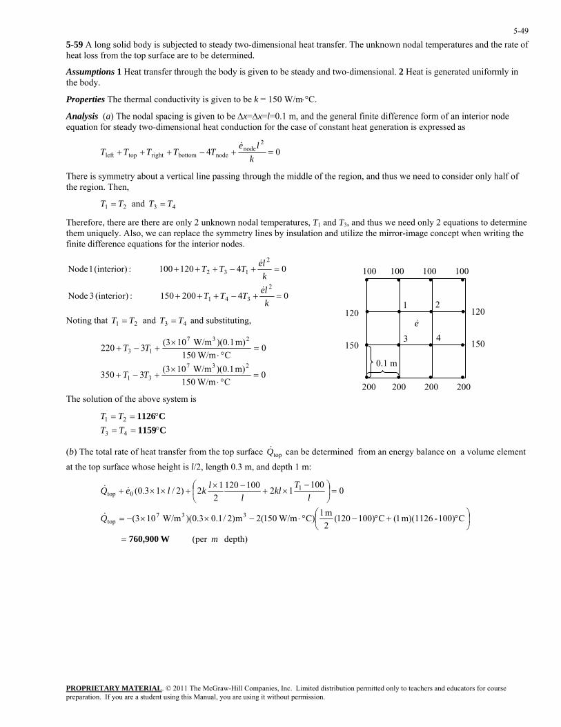
PROPRIETARY MATERIAL. © 2011 The McGraw-Hill Companies, Inc. Limited distribution permitted only to teachers and educators for course preparation. If you are a student using this Manual, you are using it without permission.
5-49
5-59 A long solid body is subjected to steady two-dimensional heat transfer. The unknown nodal temperatures and the rate of heat loss from the top surface are to be determined.
Assumptions 1 Heat transfer through the body is given to be steady and two-dimensional. 2 Heat is generated uniformly in the body.
Properties The thermal conductivity is given to be k = 150 W/m⋅°C.
Analysis (a) The nodal spacing is given to be ∆x=∆x=l=0.1 m, and the general finite difference form of an interior node equation for steady two-dimensional heat conduction for the case of constant heat generation is expressed as
042
nodenodebottomrighttopleft k
There is symmetry
=+−+++le
TTTTT&
about a vertical line passing through the middle of the region, and thus we need to consider only half of the region. Then,
lines by insulation and utilize the mirror-image concept when writing the fi te difference equations for the interior nodes.
4321 and TTTT ==
Therefore, there are there are only 2 unknown nodal temperatures, T1 and T3, and thus we need only 2 equations to determine them uniquely. Also, we can replace the symmetry
ni
04200150 :(interior) 3 Node ++
01100 :ior)
2
341
2
=+−+
=+
kleTTT
kle
&
&
Noting that 21 and TTTT = and substituting,
420(inter 1 Node 132 +−++ TTT
43 =
0C W/m150
m) )(0.1 W/m103(
0C W/m150
3220
237
13
×
=°⋅
+−+ TT
3350
m) )(0.1 W/m103(
31
237
=°⋅
+−+
×
TT
The solution of the above system is
(b) The total rate of heat transfer from the top surface can be determined from an energy balance on a volume element at the top surface whose height is l/2, length 0.3 m, and depth 1 m:
• • • •
• • • •
• • • •
• • • •100 100 100 100
120 3
1 2
0.1 m
200 200 200 200
120 1504
e&
150
C1159C1126°==°==
43
21
TTTT
topQ&
depth) (per
C100)-m)(1126 1(C)100120(2m 1)C W/m150(2m)2/1.03.0)( W/m103(
0100
121001202
12)2/13.0(
337top
10top
m
Q
lT
kll
lkleQ
W760,900=
⎟⎠⎞
⎜⎝⎛ °+°−°⋅−××−=
=⎟⎠
⎞⎜⎝
⎛ −×+
−×+××+
&
&&
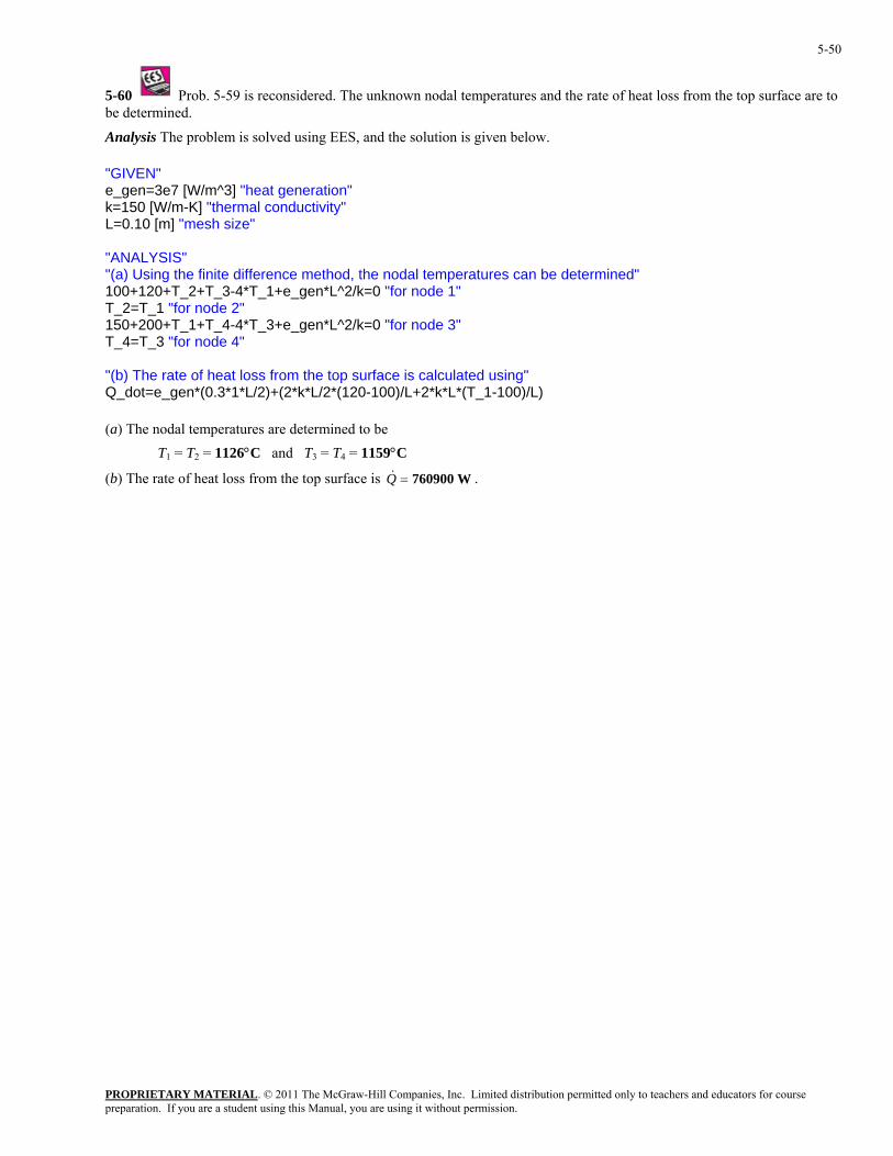
PROPRIETARY MATERIAL. © 2011 The McGraw-Hill Companies, Inc. Limited distribution permitted only to teachers and educators for course preparation. If you are a student using this Manual, you are using it without permission.
5-50
5-60 Prob. 5-59 is reconsidered. The unknown nodal temperatures and the rate of heat loss from the top surface are to
nalysis The problem is solved using EES, and the solution is given below.
conductivity"
atures can be determined"
_3+e_gen*L^2/k=0 "for node 3"
_dot=e_gen*(0.3*1*L/2)+(2*k*L/2*(120-100)/L+2*k*L*(T_1-100)/L)
(a) The n°C
) The rate of heat loss from the top surface is
be determined.
A "GIVEN" e_gen=3e7 [W/m^3] "heat generation"k=150 [W/m-K] "thermal L=0.10 [m] "mesh size" "ANALYSIS" "(a) Using the finite difference method, the nodal temper100+120+T_2+T_3-4*T_1+e_gen*L^2/k=0 "for node 1" T_2=T_1 "for node 2" 150+200+T_1+T_4-4*TT_4=T_3 "for node 4" "(b) The rate of heat loss from the top surface is calculated using" Q
odal temperatures are determined to be T1 = T2 = 1126°C and T3 = T4 = 1159
W760900=Q& . (b
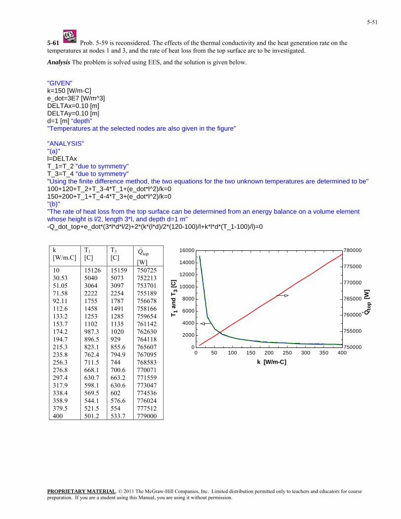
PROPRIETARY MATERIAL. © 2011 The McGraw-Hill Companies, Inc. Limited distribution permitted only to teachers and educators for course preparation. If you are a student using this Manual, you are using it without permission.
5-51
5-61 Prob. 5-59 is reconsidered. The effects of the thermal conductivity and the heat generation rate on the
nalysis The problem is solved using EES, and the solution is given below.
]
s at the selected nodes are also given in the figure"
"
equations for the two unknown temperatures are determined to be"
_dot_top+e_dot*(3*l*d*l/2)+2*(k*(l*d)/2*(120-100)/l+k*l*d*(T_1-100)/l)=0
.C]
temperatures at nodes 1 and 3, and the rate of heat loss from the top surface are to be investigated.
A
"GIVEN" k=150 [W/m-C] e_dot=3E7 [W/m^3DELTAx=0.10 [m] DELTAy=0.10 [m] d=1 [m] “depth" "Temperature "ANALYSIS"(a)" l=DELTAx T_1=T_2 "due to symmetry" T_3=T_4 "due to symmetry" "Using the finite difference method, the two 100+120+T_2+T_3-4*T_1+(e_dot*l^2)/k=0 150+200+T_1+T_4-4*T_3+(e_dot*l^2)/k=0 "(b)" "The rate of heat loss from the top surface can be determined from an energy balance on a volume element whose height is l/2, length 3*l, and depth d=1 m" -Q
k [W/m
T1 [C]
T3 [C]
topQ& [W]
10 30.53 51.05 71.58 92.11 112.6 133.2 153.7 174.2 194.7 215.3 235.8 256.3 276.8 297.4 317.9 338.4 358.9 379.5 400
501.2
533.7 779000
151265040 3064 2222 1755 1458 1253 1102 987.3 896.5 823.1 762.4 711.5 668.1 630.7 598.1 569.5 544.1 521.5
151595073 3097 2254 1787 1491 1285 1135 1020 929 855.6 794.9 744 700.6 663.2 630.6 602 576.6 554
750725 752213 753701 755189 756678 758166 759654 761142 762630 764118 765607 767095 768583 770071 771559 773047 774536 776024 777512
0 50 100 150 200 250 300 350 4000
2000
4000
6000
8000
10000
12000
14000
16000
750000
755000
760000
765000
770000
775000
780000
T 1 a
nd T
3 [C
]
Qto
p [W
]k [W/m-C]
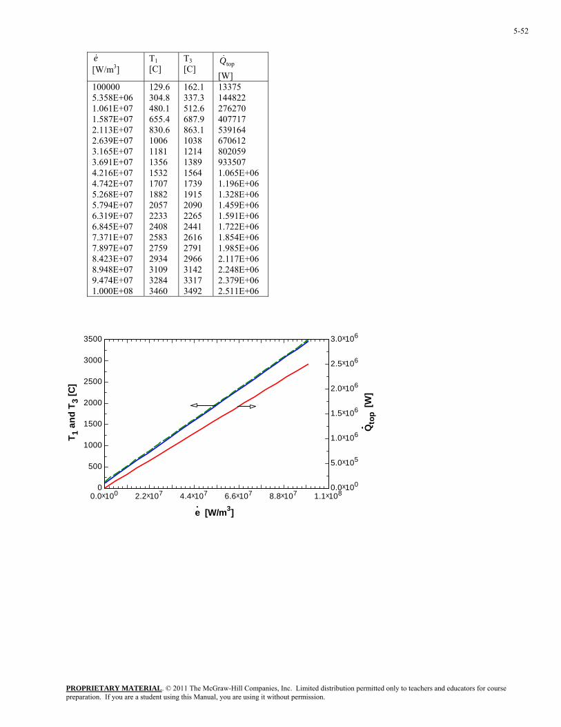
PROPRIETARY MATERIAL. © 2011 The McGraw-Hill Companies, Inc. Limited distribution permitted only to teachers and educators for course preparation. If you are a student using this Manual, you are using it without permission.
5-52
e& [W/m3]
T1 [C]
T3 [C]
topQ& [W]
100000 5.358E+06 1.061E+07 1.587E+07 2.113E+07 2.639E+07 3.165E+07 3.691E+07 4.216E+07 4.742E+07 5.268E+07 5.794E+07 6.319E+07 6.845E+07 7.371E+07 7.897E+07 8.423E+07 8.948E+07 9.474E+07 1.000E+08
129.6 304.8 480.1 655.4 830.6 1006 1181 1356 1532 1707 1882 2057 2233 2408 2583 2759 2934 3109 3284 3460
162.1 337.3 512.6 687.9 863.1 1038 1214 1389 1564 1739 1915 2090 2265 2441 2616 2791 2966 3142 3317 3492
13375 144822 276270 407717 539164 670612 802059 933507 1.065E+06 1.196E+06 1.328E+06 1.459E+06 1.591E+06 1.722E+06 1.854E+06 1.985E+06 2.117E+06 2.248E+06 2.379E+06 2.511E+06
0.0x100 2.2x10⁷ 4.4x10⁷ 6.6x10⁷ 8.8x10⁷ 1.1x1080
500
1000
1500
2000
2500
3000
3500
0.0x100
5.0x10⁵
1.0x10⁶
1.5x10⁶
2.0x10⁶
2.5x10⁶
3.0x10⁶
e [W/m3]
Qto
p [W
]
T 1 a
nd T
3 [C
]
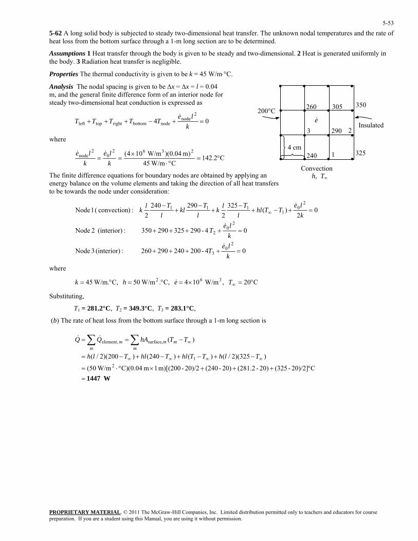
PROPRIETARY MATERIAL. © 2011 The McGraw-Hill Companies, Inc. Limited distribution permitted only to teachers and educators for course preparation. If you are a student using this Manual, you are using it without permission.
5-53
5-62 A long solid body is subjected to steady two-dimensional heat transfer. The unknown nodal temperatures and the rate of heat loss from the bottom surface through a 1-m long section are to be determined.
Assumptions 1 Heat transfer through the body is given to be steady and two-dimensional. 2 Heat is generated uniformly in the body. 3 Radiation heat transfer is negligible.
Properties The thermal conductivity is given to be k = 45 W/m⋅°C.
Analysis The nodal spacing is given to be ∆x = ∆x = l = 0.04 m, and the general finite difference form of an interior node for steady two-dimensional heat conduction is expressed as
042
nodenodebottomrighttopleft =+−+++
kle
TTTTT&
where
C2.142C W/m45 °⋅kk
The finite difference equations for boundary nodes are obtained by applying an energy balance on the volume elements and t
)m 04.0)( W/m104( 23620
2de °=
×==
lele &&
aking the direction of all heatto be towards the node under consideration:
no
transfers
04-200240290260 :(interior) 3 Node
0 4-290325290350 :(interior) 2 Node
02
)(325
2290240
2 :)convection ( 1 Node
20
3
20
2
20
1111
=++++
=++++
=+−+−
+−
+−
∞
kle
T
kle
T
kle
TThll
Tlkl
Tkl
lTlk
&
&
&
where
5 362 °=×=°=° ∞Teh &
Substitut
(b) The rate of heat loss from the bottom surface through a 1-m long section is
h, T∞
Insulated
• • • •
• • • •
• • • •
• • • •
240
200°C350260 305
2903
1
2
4 cm 325
Convection
e&
4=k C20 , W/m104 C,. W/m50 C, W/m.
ing,
T1 = 281.2°C, T2 = 349.3°C, T3 = 283.1°C,
W1447=°+++×°⋅=
−+−+−+−=
−==
∞∞∞∞
∞∑∑
C20)/2]-(32520)-(281.220)-(24020)/2-m)[(200 1 m C)(0.04 W/m50(
)325)(2/()()240()200)(2/(
)(
21
surface, element,
TlhTThlThlTlh
TThAQQm
mmm
m&&
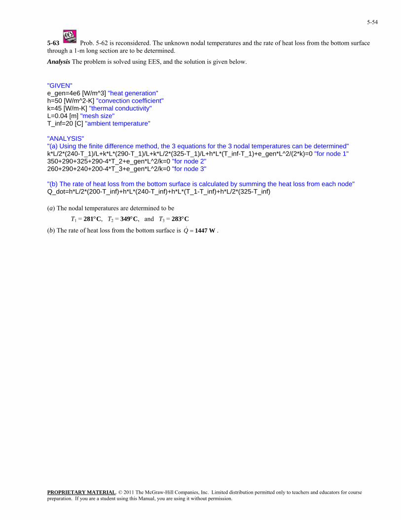
PROPRIETARY MATERIAL. © 2011 The McGraw-Hill Companies, Inc. Limited distribution permitted only to teachers and educators for course preparation. If you are a student using this Manual, you are using it without permission.
5-54
5-63 Prob. 5-62 is reconsidered. The unknown nodal temperatures and the rate of heat loss from the bottom surface
nalysis The problem is solved using EES, and the solution is given below.
nt"
*L*(T_inf-T_1)+e_gen*L^2/(2*k)=0 "for node 1"
e heat loss from each node" _dot=h*L/2*(200-T_inf)+h*L*(240-T_inf)+h*L*(T_1-T_inf)+h*L/2*(325-T_inf)
(a) The nC
) The rate of heat loss from the bottom surface is
through a 1-m long section are to be determined.
A "GIVEN" e_gen=4e6 [W/m^3] "heat generation" h=50 [W/m^2-K] "convection coefficiek=45 [W/m-K] "thermal conductivity"L=0.04 [m] "mesh size" T_inf=20 [C] "ambient temperature" "ANALYSIS" "(a) Using the finite difference method, the 3 equations for the 3 nodal temperatures can be determined" k*L/2*(240-T_1)/L+k*L*(290-T_1)/L+k*L/2*(325-T_1)/L+h350+290+325+290-4*T_2+e_gen*L^2/k=0 "for node 2" 260+290+240+200-4*T_3+e_gen*L^2/k=0 "for node 3" "(b) The rate of heat loss from the bottom surface is calculated by summing thQ
odal temperatures are determined to be T1 = 281°C, T2 = 349°C, and T3 = 283°
W1447=Q& . (b
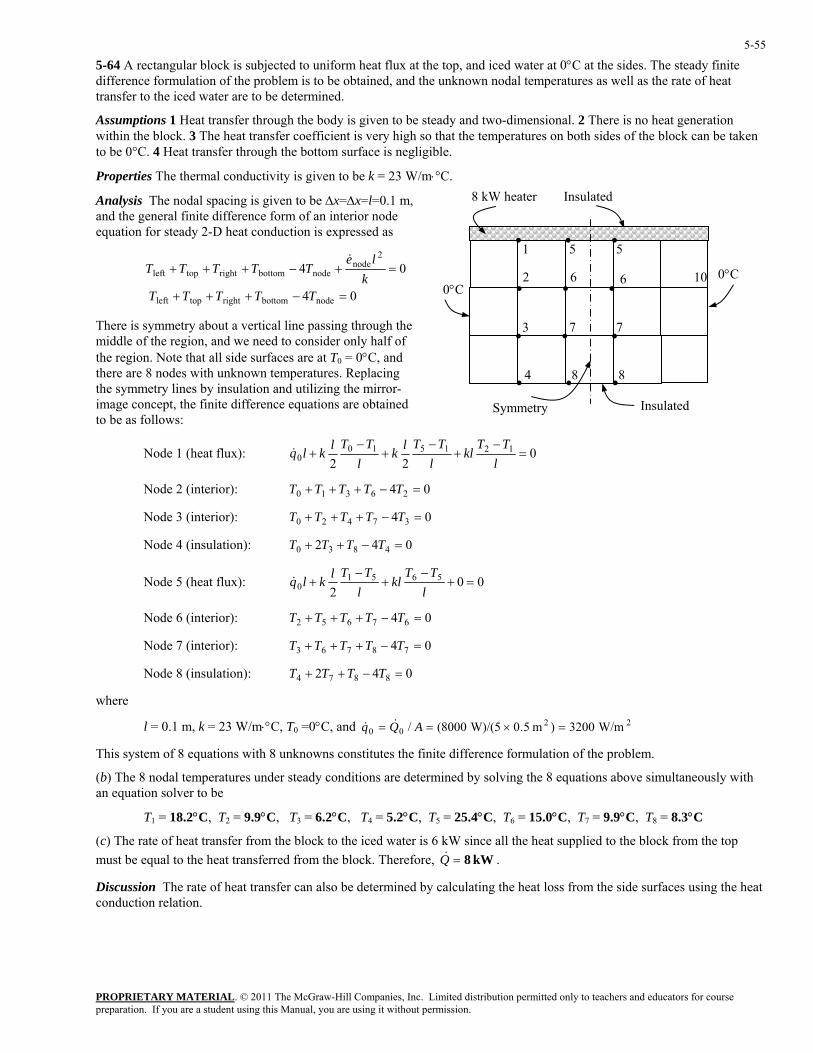
PROPRIETARY MATERIAL. © 2011 The McGraw-Hill Companies, Inc. Limited distribution permitted only to teachers and educators for course preparation. If you are a student using this Manual, you are using it without permission.
5-55
5-64 A rectangular block is subjected to uniform heat flux at the top, and iced water at 0°C at the sides. The steady finite difference formulation of the problem is to be obtained, and the unknown nodal temperatures as well as the rate of heat transfer to the iced water are to be determined.
Assumptions 1 Heat transfer through the body is given to be steady and two-dimensional. 2 There is no heat generation within the block. 3 The heat transfer coefficient is very high so that the temperatures on both sides of the block can be taken to be 0°C. 4 Heat transfer through the bottom surface is negligible.
Properties The thermal conductivity is given to be k = 23 W/m⋅°C.
0°C62 6 10
Insulated
3 7 7
0°C
8 kW heater Insulated
• • •
• • •
• • •
• • •4 8 8
1 5 5
Symmetry
Analysis The nodal spacing is given to be ∆x=∆x=l=0.1 m, and the general finite difference form of an interior node equation for steady 2-D heat conduction is expressed as
04 nodebottomrighttopleft
nodebottomrighttopleft
=−+++ TTTTTk
There is symmetry about a vertical line passing through thmiddle of the region, and we need to consider only half ofthe region. Note that all side surfaces are at T
042
node =+−+++le
TTTTT&
e
with unknown temperatures. Replacing the symmetry lines by insulation and utilizing the mirror-image co rence equations are obtained to be as fo
0 = 0°C, and there are 8 nodes
ncept, the finite diffellows:
022
1215100 =
−+
−+
−+
lTT
kll
TTlkl
TTlkNode 1 (heat flux): lq&
Node 2 (interior): 04 26310 =−+++ TTTTT
Node 3 (interior): 04 37420 =−+++ TTTTT
042 4830 =−++ TTTT Node 4 (insulation):
002
56510 =+
−+
−+
lTT
kll
TTlklq& Node 5 (heat flux):
Node 6 (interior): 2 04 6765 =−+++ TTTTT
Node 7 (interior): 04 78763 =−+++ TTTTT
Node 8 (insulation): 2 874 ++ TTT 04 8 =− T
s the finite difference formulation of the problem.
) The sly with
= 5.4°C, T6 = 15.0°C, T7 = 9.9°C, T8 = 8.3°C
eat transferred from the block. Therefore,
Discussion The rate of heat transfer can also be determined by calculating the heat loss from the side surfaces using the heat conduction relation.
where
l = 0.1 m, k = 23 W/m⋅°C, T0 =0°C, and 2200 W/m3200)m 5.0 W)/(58000(/ =×== AQq &&
This system of 8 equations with 8 unknowns constitute
(b 8 nodal temperatures under steady conditions are determined by solving the 8 equations above simultaneouan equation solver to be
T1 = 18.2°C, T2 = 9.9°C, T3 = 6.2°C, T4 = 5.2°C, T5 2
(c) The rate of heat transfer from the block to the iced water is 6 kW since all the heat supplied to the block from the top must be equal to the h kW 8=Q& .
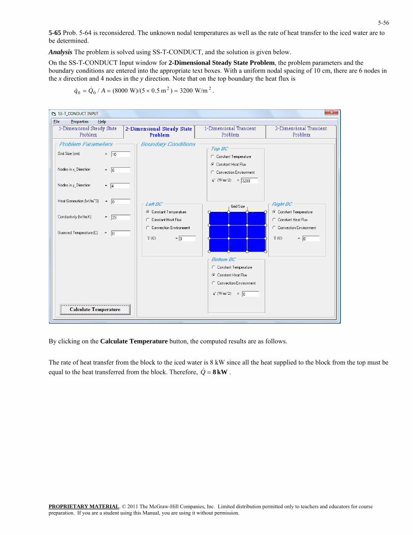
PROPRIETARY MATERIAL. © 2011 The McGraw-Hill Companies, Inc. Limited distribution permitted only to teachers and educators for course preparation. If you are a student using this Manual, you are using it without permission.
5-56
5-65 Prob. 5-64 is reconsidered. The unknown nodal temperatures as well as the rate of heat transfer to the iced water are to be determined.
Analysis The problem is solved using SS-T-CONDUCT, and the solution is given below. On the SS-T-CONDUCT Input window for 2-Dimensional Steady State Problem, the problem parameters and the boundary conditions are entered into the appropriate text boxes. With a uniform nodal spacing of 10 cm, there are 6 nodes in the x direction and 4 nodes in the y direction. Note that on the top boundary the heat flux is
2200 W/m3200)m 5.0 W)/(58000(/ =×== AQq && .
By clicking on the Calculate Temperature button, the computed results are as follows. The rate of heat transfer from the block to the iced water is 8 kW since all the heat supplied to the block from the top must be equal to the heat transferred from the block. Therefore, kW 8=Q& .
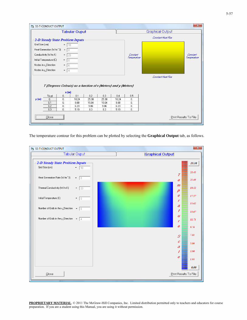
PROPRIETARY MATERIAL. © 2011 The McGraw-Hill Companies, Inc. Limited distribution permitted only to teachers and educators for course preparation. If you are a student using this Manual, you are using it without permission.
5-57
The temperature contour for this problem can be plotted by selecting the Graphical Output tab, as follows.
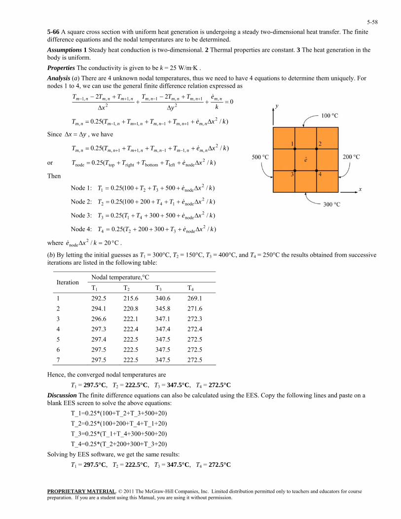
PROPRIETARY MATERIAL. © 2011 The McGraw-Hill Companies, Inc. Limited distribution permitted only to teachers and educators for course preparation. If you are a student using this Manual, you are using it without permission.
5-58
5-66 A square cross section with uniform heat generation is undergoing a steady two-dimensional heat transfer. The finite difference equations and the nodal temperatures are to be determined. Assumptions 1 Steady heat conduction is two-dimensional. 2 Thermal properties are constant. 3 The heat generation in the body is uniform. Properties The conductivity is given to be k = 25 W/m·K . Analysis (a) There are 4 unknown nodal temperatures, thus we need to have 4 equations to determine them uniquely. For nodes 1 to 4, we can use the general finite difference relation expressed as
022 ,
21 , ,1 ,
2 ,1 , ,1 =+
∆
+−+
∆
+− +−+−
ke
y
TTT
x
TTT nmnmnmnmnmnmnm &
25.0 ,T nm = )/( 2 ,1 ,1 , ,1 ,1 kxeTTTT nmnmnmnmnm ∆++++ +−+− &
ince , we have
hen
Node 4: kxeTTT ∆++++= &
(b) By letting th 300°C, T2 = 150°C, T3 = 400°C, and T4 = 250°C the results obtained from successive iterations are listed in the following table:
temp °C
yx ∆=∆S
)/(25.0 2 , ,11 , ,11 , , kxeTTTTT nmnmnmnmnmnm ∆++++= −−++ &
)/(25.0 2nodeleftbottomrighttopnode kxeTTTTT ∆++++= & or
T
)/500100(25.0 2node321 kxeTTT ∆++++= & Node 1:
Node 2: )/200100(25.0 2node142 kxeTTT ∆++++= &
)/500300(25.0 2node413 kxeTTT ∆++++= & Node 3:
)/300200(25.0 2 node324
where C 20/2node °=∆ kxe& .
e initial guesses as T1 =
Nodal erature,Iteration
T1 T2 T3 T4
1 292.5 215.6 340.6 269.1 2 294.1 220.8 345.8 271.6 3 296.6 222.1 347.1 272.3 4 297.3 222.4 347.4 272.4 5 297.4 222.5 347.5 272.5 6 297.5 222.5 347.5 272.5 7 297.5 222.5 347.5 272.5
Hence, the converged nodal temperatures are T1 = 297.5°C, T2 = 222.5°C, T3 = 347.5°C, T4 = 272.5°C
also be calculated using the EES. Copy the following lines and paste on a :
Solving by EES software, we get the same results: T1 = 297.5°C, T2 = 222.5°C, T3 = 347.5°C, T4 = 272.5°C
Discussion The finite difference equations canblank EES screen to solve the above equations T_1=0.25*(100+T_2+T_3+500+20) T_2=0.25*(100+200+T_4+T_1+20) T_3=0.25*(T_1+T_4+300+500+20) T_4=0.25*(T_2+200+300+T_3+20)
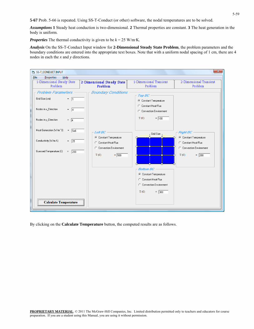
PROPRIETARY MATERIAL. © 2011 The McGraw-Hill Companies, Inc. Limited distribution permitted only to teachers and educators for course preparation. If you are a student using this Manual, you are using it without permission.
5-59
5-67 Prob. 5-66 is repeated. Using SS-T-Conduct (or other) software, the nodal temperatures are to be solved.
Assumptions 1 Steady heat conduction is two-dimensional. 2 Thermal properties are constant. 3 The heat generation in the body is uniform.
Properties The thermal conductivity is given to be k = 25 W/m·K.
Analysis On the SS-T-Conduct Input window for 2-Dimensional Steady State Problem, the problem parameters and the boundary conditions are entered into the appropriate text boxes. Note that with a uniform nodal spacing of 1 cm, there are 4 nodes in each the x and y directions.
By clicking on the Calculate Temperature button, the computed results are as follows.
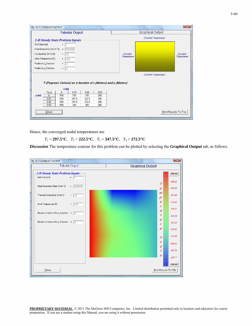
PROPRIETARY MATERIAL. © 2011 The McGraw-Hill Companies, Inc. Limited distribution permitted only to teachers and educators for course preparation. If you are a student using this Manual, you are using it without permission.
5-60
Hence, the converged nodal temperatures are
T1 = 297.5°C, T2 = 222.5°C, T3 = 347.5°C, T4 = 272.5°C
Discussion The temperature contour for this problem can be plotted by selecting the Graphical Output tab, as follows.
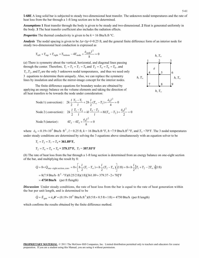
PROPRIETARY MATERIAL. © 2011 The McGraw-Hill Companies, Inc. Limited distribution permitted only to teachers and educators for course preparation. If you are a student using this Manual, you are using it without permission.
5-61
5-68E A long solid bar is subjected to steady two-dimensional heat transfer. The unknown nodal temperatures and the rate of heat loss from the bar through a 1-ft long section are to be determined.
Assumptions 1 Heat transfer through the body is given to be steady and two-dimensional. 2 Heat is generated uniformly in the body. 3 The heat transfer coefficient also includes the radiation effects.
Properties The thermal conductivity is given to be k = 16 Btu/h.ft⋅°C.
Analysis The nodal spacing is given to be ∆x=∆y=l=0.25 ft, and the general finite difference form of an interior node for steady two-dimensional heat conduction is expressed as
042
nodenodebottomrighttopleft =+−+++
kle
TTTTT&
• • •
4 5 6
• •
• • •h, T∞
1 2 3
7 8 9
h, T∞ h, T∞
h, T∞
e&
(a) There is symmetry about the vertical, horizontal, and diagonal lines passing through the center. Therefore, 3T 971 TTT == and T= 864 TTT2 === , and
521 and ,, TTT are the only 3 unknown nodal temperatures, and thus we need only3 equations to determine them uniquely. Also, we can replace the symmetry lines by insulation and utilize the mirror-image c
oncept for the interior nodes.
The finite difference equations for boundary nodes are obtained by applying an energy balance on the volume elements and taking the direction of all heat transfers to be towards the node under consideration:
044 :(interior) 5 Node
02
)( 2
2 :)convection ( 2 Node
04
)(2
22
2 :)convection ( 1 Node
20
52
20
22521
20
112
=+−
=+−+−
+−
=+−+−
∞
∞
kle
TT
leTThl
lTT
kll
TTlk
leTTlh
lTTlk
&
&
&
where 350 ftBtu/h 1019.0 ⋅×= , l = 0.25 ft, k = 16 Btu/h.ft⋅°F, h =7.9 Btu/h.fte& 2⋅°F, and T∞ =70°F. The 3 nodal temperatures
under steady conditions are determined by solving the 3 equations above simultaneously with an equation solver to be
T T5 = 397.93°F
9731 TTTT === = 361.89°F,
864 TTT === = 379.37°F, 2
(b) The rate of heat loss from the bar through a 1-ft long section is determined from an energy balance on one-eight section of the bar, and multiplying the result by 8:
[ ]
flength)ft per (F70]2-37.379ft)[361.89 ft)(1 F)(0.25/2ftBtu/h 9.7(8
ft) 1()22
8ft) 1()(2
)(2
88
2
2121conv section,eight one
Btu/h 4750=°×+°⋅⋅=
−+×=⎥⎦⎤
⎢⎣⎡ −+−×=×= ∞∞∞− TTTlhTTlhTTlhQQ &&
Discussion Under steady conditions, the rate of heat loss from the bar is equal to the rate of heat generation within the bar per unit length, and is determined to be
length)ft per (Btu/h 4750ft) 1 ft 0.5 ft 5.0)(Btu/h.ft 1019.0( 350gen =×××== VeEQ &&&
which confirms the results obtained by the finite difference method.
=
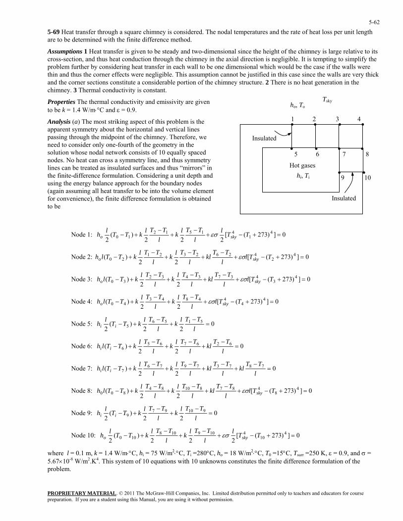
PROPRIETARY MATERIAL. © 2011 The McGraw-Hill Companies, Inc. Limited distribution permitted only to teachers and educators for course preparation. If you are a student using this Manual, you are using it without permission.
5-62
5-69 Heat transfer through a square chimney is considered. The nodal temperatures and the rate of heat loss per unit length are to be determined with the finite difference method.
Assumptions 1 Heat transfer is given to be steady and two-dimensional since the height of the chimney is large relative to its cross-section, and thus heat conduction through the chimney in the axial direction is negligible. It is tempting to simplify the problem further by considering heat transfer in each wall to be one dimensional which would be the case if the walls were thin and thus the corner effects were negligible. This assumption cannot be justified in this case since the walls are very thick and the corner sections constitute a considerable portion of the chimney structure. 2 There is no heat generation in the chimney. 3 Thermal conductivity is constant.
• • • • 1 2 3 4
Tskyho, To
• • • •
• •
5 6 7 8
9 10hi, Ti
Insulated
Insulated
Hot gases
Properties The thermal conductivity and emissivity are given to be k = 1.4 W/m⋅°C and ε = 0.9.
Analysis (a) The most striking aspect of this problem is the apparent symmetry about the horizontal and vertical lines passing through the midpoint of the chimney. Therefore, we need to consider only one-fourth of the geometry in the solution whose nodal network consists of 10 equally spaced nodes. No heat can cross a symmetry line, and thus symmetry lines can be treated as insulated surfaces and thus “mirrors” in the finite-difference formulation. Considering a unit depth and using the energy balance approach for the boundary nodes (again assuming all heat transfer to be into the volume element for convenience), the finite difference formulation is obtained to be
Node 1: 0])273([222
)(2
41
4151210 =+−+
−+
−+− TTl
lTTlk
lTTlkTTlh skyo εσ
Node 2: 0])273([22
)( 42
426232120 =+−+
−+
−+
−+− TTl
lTT
kll
TTlkl
TTlkTTlh skyo εσ
Node 3: 0])273([22
)( 43
437343230 =+−+
−+
−+
−+− TTl
lTT
kll
TTlkl
TTlkTTlh skyo εσ
Node 4: 0])273([l22
)( 44
4484340 =+−+
−+
−+− TT
lTTlk
lTTlkTTlh skyo εσ
022
)(2
51565 =
−+
−+−
lTTlk
lTTlkTTlh ii Node 5:
022
)( 6267656 =
−+
−+
−+−
lTT
kll
TTlkl
TTlkTTlh ii Node 6:
022
)( 787379767 =
−+
−+
−+
−+−
lTT
kll
TTkl
lTTlk
lTTlkTTlh ii Node 7:
(TlhNode 8: 0])273([22
) 48
48781084800 =+−+
−+
−+
−+− TTl
lTT
kll
TTlkl
TTlkT skyεσ
Node 9: 022
)(2
910979 =
−+
−+−
lTTlk
lTTlkTTlh ii
0])273([222
)(2
410
4109108100 =+−+
−+
−+− TTl
lTTlk
lTTlkTTlh skyo εσ Node 10:
where l = 0.1 m, k = 1.4 W/m⋅°C, hi = 75 W/m2⋅°C, Ti =280°C, ho = 18 W/m2⋅°C, T0 =15°C, Tsurr =250 K, ε = 0.9, and σ = 5.67×10⁻⁸ W/m2.K4. This system of 10 equations with 10 unknowns constitutes the finite difference formulation of the problem.
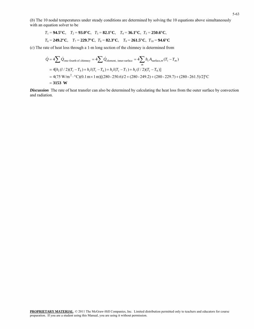
PROPRIETARY MATERIAL. © 2011 The McGraw-Hill Companies, Inc. Limited distribution permitted only to teachers and educators for course preparation. If you are a student using this Manual, you are using it without permission.
5-63
(b) The 10 nodal temperatures under steady conditions are determined by solving the 10 equations above simultaneously with an equation solver to be
T1 = 94.5°C, T2 = 93.0°C, T3 = 82.1°C, T4 = 36.1°C, T5 = 250.6°C,
T6 = 249.2°C, T7 = 229.7°C, T8 = 82.3°C, T9 = 261.5°C, T10 = 94.6°C
(c) The rate of heat loss through a 1-m long section of the chimney is determined from
W3153=°+++×°⋅=
−+−+−+−=
−=== ∑∑∑
C261.5)/2]-(280229.7)-(280249.2)-(280250.6)/2-m)[(280 1 m C)(0.1 W/m75(4
)])(2/()()())(2/([4
)(444
29765
surface,surfaceinner element,chimney offourth -one
TTlhTTlhTTlhTTlh
TTAhQQQ
iiiiiiii
mmimi
&&&
Discussion The rate of heat transfer can also be determined by calculating the heat loss from the outer surface by convection and radiation.
PROPRIETARY MATERIAL. © 2011 The McGraw-Hill Companies, Inc. Limited distribution permitted only to teachers and educators for course preparation. If you are a student using this Manual, you are using it without permission.
5-64
5-70 Heat transfer through a square chimney is considered. The nodal temperatures and the rate of heat loss per unit length are to be determined with the finite difference method.
Assumptions 1 Heat transfer is given to be steady and two-dimensional since the height of the chimney is large relative to its cross-section, and thus heat conduction through the chimney in the axial direction is negligible. It is tempting to simplify the problem further by considering heat transfer in each wall to be one dimensional which would be the case if the walls were thin and thus the corner effects were negligible. This assumption cannot be justified in this case since the walls are very thick and the corner sections constitute a considerable portion of the chimney structure. 2 There is no heat generation in the chimney. 3 Thermal conductivity is constant. 4 Radiation heat transfer is negligible.
• • • • 1 2 3 4
ho, To
• • • •
• •
5 6 7 8
9 10hi, Ti
Insulated
Insulated
Hot gases
Properties The thermal conductivity of chimney is given to be k = 1.4 W/m⋅°C.
Analysis (a) The most striking aspect of this problem is the apparent symmetry about the horizontal and vertical lines passing through the midpoint of the chimney. Therefore, we need to consider only one-fourth of the geometry in the solution whose nodal network consists of 10 equally spaced nodes. No heat can cross a symmetry line, and thus symmetry lines can be treated as insulated surfaces and thus “mirrors” in the finite-difference formulation. Considering a unit depth and using the energy balance approach for the boundary nodes (again assuming all heat transfer to be into the volume element for convenience), the finite difference formulation is obtained to be
Node 1: 022
)(2
151210 =
−+
−+−
lTTlk
lTTlkTTlho
022
)( 26232120 =
−+
−+
−+−
lTT
kll
TTlkl
TTlkTTlho Node 2:
022
)( 37343230 =
−+
−+
−+−
lTT
kll
TTlkl
TTlkTTlho Node 3:
022
)( 484340 =
−+
−+−
lTTlk
lTTlkTTloh Node 4:
022
)(2
51565 =
−+
−+−
lTTlk
lTTlkTTlh ii Node 5:
022
)( 6267656 =
−+
−+
−+−
lTT
kll
TTlkl
TTlkTTlh ii Node 6:
(lNode 7: 022
) 787379767 =
−+
−+
−+
−+−
lTT
kll
TTkl
lTTlk
lTTlkTTh ii
022
)( 87 −h 8108480 =+
−+
−+−
lTT
kll
TTlkl
TTlkTTlo Node 8:
Node 9: 022
)(2
910979 =
−+
−+−
lTTlk
lTTlkTTlh ii
022
)(2
109108100 =
−+
−+−
lTTlk
lTTlkTTlho Node 10:
where l = 0.1 m, k = 1.4 W/m⋅°C, hi = 75 W/m2⋅°C, Ti =280°C, ho = 18 W/m2⋅°C, T0 =15°C, and σ = 5.67×10⁻⁸ W/m2.K4. This system of 10 equations with 10 unknowns constitutes the finite difference formulation of the problem.
PROPRIETARY MATERIAL. © 2011 The McGraw-Hill Companies, Inc. Limited distribution permitted only to teachers and educators for course preparation. If you are a student using this Manual, you are using it without permission.
5-65
−== ∑∑∑
C263.7)/2]-(280235.2)-(280253.0)-(280254.4)/2-m)[(280 1 m C)(0.1 W/m75(4
)])(2/()()())(2/(
)(444
29765 TTlhTTlhTTlhTTl
TTAhQQQ
iiiiiii
&&&
Discussion The rate of heat transfer can also be determined by calculating the heat loss from the outer surface by convection.
(b) The 10 nodal temperatures under steady conditions are determined by solving the 10 equations above simultaneously with an equation solver to be
T1 = 118.8°C, T2 = 116.7°C, T3 = 103.4°C, T4 = 53.7°C, T5 = 254.4°C,
T6 = 253.0°C, T7 = 235.2°C, T8 = 103.5°C, T9 = 263.7°C, T10 = 117.6°C
(c) The rate of heat loss through a 1-m long section of the chimney is determined from
= [4
surface,surfaceinner element,chimney offourth -one
hi
mmimi
W2783=°+++×°⋅=
−+−+−+−
=
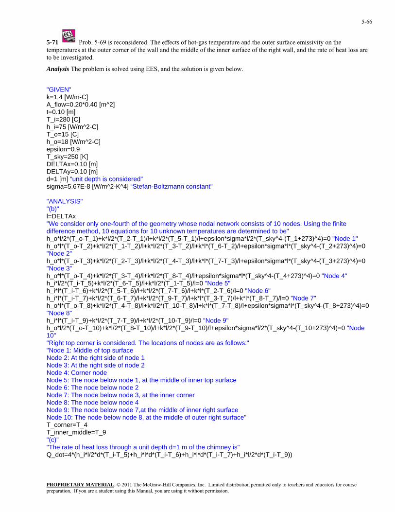
PROPRIETARY MATERIAL. © 2011 The McGraw-Hill Companies, Inc. Limited distribution permitted only to teachers and educators for course preparation. If you are a student using this Manual, you are using it without permission.
5-66
5-71 Prob. 5-69 is reconsidered. The effects of hot-gas temperature and the outer surface emissivity on the temperatures at the outer corner of the wall and the middle of the inner surface of the right wall, and the rate of heat loss are to be investigated.
Analysis The problem is solved using EES, and the solution is given below.
"GIVEN" k=1.4 [W/m-C] A_flow=0.20*0.40 [m^2] t=0.10 [m] T_i=280 [C] h_i=75 [W/m^2-C] T_o=15 [C] h_o=18 [W/m^2-C] epsilon=0.9 T_sky=250 [K] DELTAx=0.10 [m] DELTAy=0.10 [m] d=1 [m] “unit depth is considered" sigma=5.67E-8 [W/m^2-K^4] “Stefan-Boltzmann constant" "ANALYSIS" "(b)" l=DELTAx "We consider only one-fourth of the geometry whose nodal network consists of 10 nodes. Using the finite difference method, 10 equations for 10 unknown temperatures are determined to be" h_o*l/2*(T_o-T_1)+k*l/2*(T_2-T_1)/l+k*l/2*(T_5-T_1)/l+epsilon*sigma*l/2*(T_sky^4-(T_1+273)^4)=0 "Node 1" h_o*l*(T_o-T_2)+k*l/2*(T_1-T_2)/l+k*l/2*(T_3-T_2)/l+k*l*(T_6-T_2)/l+epsilon*sigma*l*(T_sky^4-(T_2+273)^4)=0 "Node 2" h_o*l*(T_o-T_3)+k*l/2*(T_2-T_3)/l+k*l/2*(T_4-T_3)/l+k*l*(T_7-T_3)/l+epsilon*sigma*l*(T_sky^4-(T_3+273)^4)=0 "Node 3" h_o*l*(T_o-T_4)+k*l/2*(T_3-T_4)/l+k*l/2*(T_8-T_4)/l+epsilon*sigma*l*(T_sky^4-(T_4+273)^4)=0 "Node 4" h_i*l/2*(T_i-T_5)+k*l/2*(T_6-T_5)/l+k*l/2*(T_1-T_5)/l=0 "Node 5" h_i*l*(T_i-T_6)+k*l/2*(T_5-T_6)/l+k*l/2*(T_7-T_6)/l+k*l*(T_2-T_6)/l=0 "Node 6" h_i*l*(T_i-T_7)+k*l/2*(T_6-T_7)/l+k*l/2*(T_9-T_7)/l+k*l*(T_3-T_7)/l+k*l*(T_8-T_7)/l=0 "Node 7" h_o*l*(T_o-T_8)+k*l/2*(T_4-T_8)/l+k*l/2*(T_10-T_8)/l+k*l*(T_7-T_8)/l+epsilon*sigma*l*(T_sky^4-(T_8+273)^4)=0 "Node 8" h_i*l*(T_i-T_9)+k*l/2*(T_7-T_9)/l+k*l/2*(T_10-T_9)/l=0 "Node 9" h_o*l/2*(T_o-T_10)+k*l/2*(T_8-T_10)/l+k*l/2*(T_9-T_10)/l+epsilon*sigma*l/2*(T_sky^4-(T_10+273)^4)=0 "Node 10" "Right top corner is considered. The locations of nodes are as follows:" "Node 1: Middle of top surface Node 2: At the right side of node 1 Node 3: At the right side of node 2 Node 4: Corner node Node 5: The node below node 1, at the middle of inner top surface Node 6: The node below node 2 Node 7: The node below node 3, at the inner corner Node 8: The node below node 4 Node 9: The node below node 7,at the middle of inner right surface Node 10: The node below node 8, at the middle of outer right surface" T_corner=T_4 T_inner_middle=T_9 "(c)" "The rate of heat loss through a unit depth d=1 m of the chimney is" Q_dot=4*(h_i*l/2*d*(T_i-T_5)+h_i*l*d*(T_i-T_6)+h_i*l*d*(T_i-T_7)+h_i*l/2*d*(T_i-T_9))
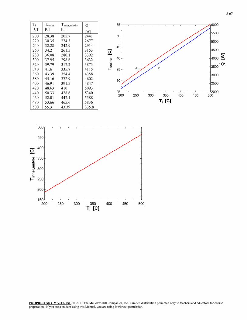
PROPRIETARY MATERIAL. © 2011 The McGraw-Hill Companies, Inc. Limited distribution permitted only to teachers and educators for course preparation. If you are a student using this Manual, you are using it without permission.
5-67
Ti [C]
Tcorner [C]
Tinner, middle [C]
Q& [W]
200 220 240 260 280 300 320 340 360 380 400 420 440 460 480 500
28.38 30.35 32.28 34.2 36.08 37.95 39.79 41.6 43.39 45.16 46.91 48.63 50.33 52.01 53.66 55.3
205.7 224.3 242.9 261.5 280.1 298.6 317.2 335.8 354.4 372.9 391.5 410 428.6 447.1 465.6 43.39
2441 2677 2914 3153 3392 3632 3873 4115 4358 4602 4847 5093 5340 5588 5836 335.8
200 250 300 350 400 450 50025
30
35
40
45
50
55
2000
2500
3000
3500
4000
4500
5000
5500
6000
Ti [C]
T cor
ner
[C]
Q [
W]
200 250 300 350 400 450 500150
200
250
300
350
400
450
500
Ti [C]
T inn
er,m
iddl
e [C
]
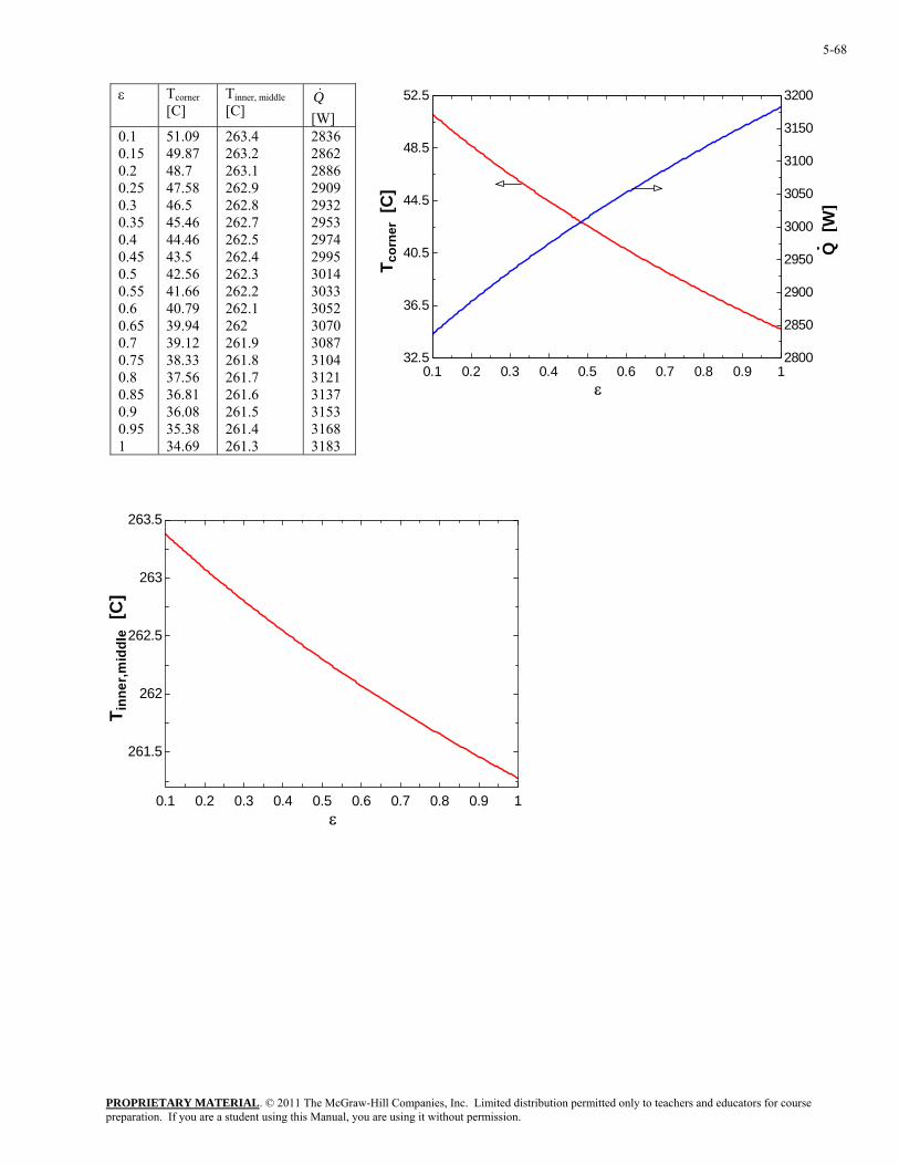
PROPRIETARY MATERIAL. © 2011 The McGraw-Hill Companies, Inc. Limited distribution permitted only to teachers and educators for course preparation. If you are a student using this Manual, you are using it without permission.
5-68
ε Tcorner
[C] Tinner, middle [C]
Q& [W]
0.1 0.15 0.2 0.25 0.3 0.35 0.4 0.45 0.5 0.55 0.6 0.65 0.7 0.75 0.8 0.85 0.9 0.95 1
51.09 49.87 48.7 47.58 46.5 45.46 44.46 43.5 42.56 41.66 40.79 39.94 39.12 38.33 37.56 36.81 36.08 35.38 34.69
263.4 263.2 263.1 262.9 262.8 262.7 262.5 262.4 262.3 262.2 262.1 262 261.9 261.8 261.7 261.6 261.5 261.4 261.3
2836 2862 2886 2909 2932 2953 2974 2995 3014 3033 3052 3070 3087 3104 3121 3137 3153 3168 3183
0.1 0.2 0.3 0.4 0.5 0.6 0.7 0.8 0.9 132.5
36.5
40.5
44.5
48.5
52.5
2800
2850
2900
2950
3000
3050
3100
3150
3200
εT c
orne
r [C
]
Q [
W]
0.1 0.2 0.3 0.4 0.5 0.6 0.7 0.8 0.9 1
261.5
262
262.5
263
263.5
ε
T inn
er,m
iddl
e [C
]
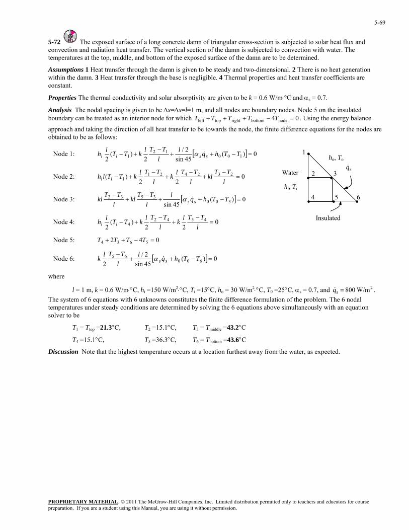
PROPRIETARY MATERIAL. © 2011 The McGraw-Hill Companies, Inc. Limited distribution permitted only to teachers and educators for course preparation. If you are a student using this Manual, you are using it without permission.
5-69
5-72 The exposed surface of a long concrete damn of triangular cross-section is subjected to solar heat flux aconvection and radiation heat transfer. The vertical section of the damn is subjected to convection with
nd water. The
damn. 3 Heat transfer through the base is negligible. 4 Thermal properties and heat transfer coefficients are
m, and all nodes are boundary nodes. N
temperatures at the top, middle, and bottom of the exposed surface of the damn are to be determined.
Assumptions 1 Heat transfer through the damn is given to be steady and two-dimensional. 2 There is no heat generationwithin theconstant.
Properties The thermal conductivity and solar absorptivity are given to be k = 0.6 W/m⋅°C and αs = 0.7.
Analysis The nodal spacing is given to be ∆x=∆x=l=1 ode 5 on the insulated boundary can be treated as an interior node for which 04 nodebottomrighttopleft =−+++ TTTTT . Using the energy balance approach and taking the direction of all h finite difference equations for the nodes are eat transfer to be towards the node, the obtained to be as follows:
[ ] 0)(45sin2/
2)(
2 10012
1 =−++−
+− TThqll
TTlkTTlh ssii &α Node 1:
Node 2: 022
)( 2324211 =
−+
−+
−+−
lTT
kll
TTlkl
TTlkTTlh ii
[ ] 0)(45sin 300
3532 =
Insulated
Water
hi, Ti
ho, To
• •
• • •
•
4 5 6
2 3
1
&qs
Node 3: −++−
+−
TThqll
TTkl
lTT
kl ss &α
Node 4: 022
)(2
45424 =
−+
−+−
lTTlk
lTTlkTTlh ii
042 5634 =−++ TTTT Node 5:
Node 6: [ ] 0)(45sin2 600
65 =−++ TThql
k ss &α
where
2/− lTTl
C, h T 2⋅°C, T0 =25°C, αs = 0.7, and The syst init formulation of the problem. The 6 nodal temperatures under steady conditions are determ ultaneously with an equation
T1 = Ttop =21.3°C, T2 =15.1°C, T3 = Tmiddle =43.2°C
T4 =15.1°C, T5 =36.3°C, T6 = Tbottom =43.6°C
Discussion Note that the highest temperature occurs at a location furthest away from the water, as expected.
2 W/m800=sq& . l = 1 m, k = 0.6 W/m⋅° i =150 W/m2⋅°C, i =15°C, ho = 30 W/mem of 6 equations with 6 unknowns constitutes the f e difference
ined by solving the 6 equations above simsolver to be
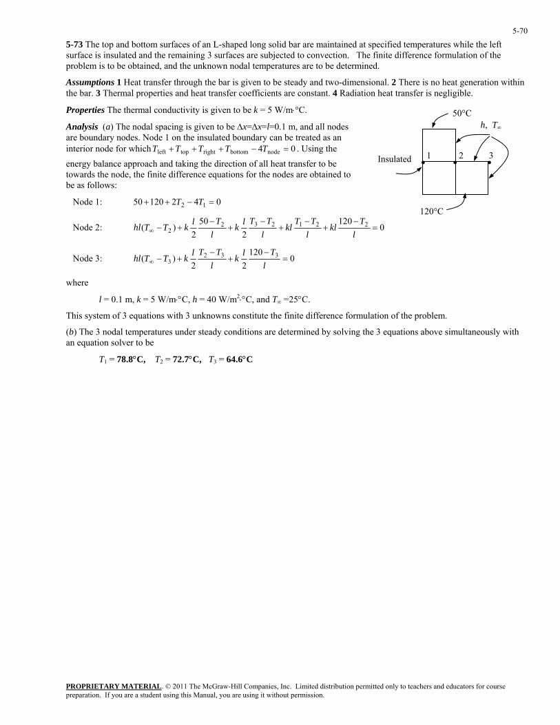
PROPRIETARY MATERIAL. © 2011 The McGraw-Hill Companies, Inc. Limited distribution permitted only to teachers and educators for course preparation. If you are a student using this Manual, you are using it without permission.
5-70
5-73 The top and bottom surfaces of an L-shaped long solid bar are maintained at specified temperatures while the left surface is insulated and the remaining 3 surfaces are subjected to convection. The finite difference formulation of the problem is to be obtained, and the unknown nodal temperatures are to be determined.
Assumptions 1 Heat transfer through the bar is given to be steady and two-dimensional. 2 There is no heat generation within the bar. 3 Thermal properties and heat transfer coefficients are constant. 4 Radiation heat transfer is negligible.
Properties The thermal conductivity is given to be k = 5 W/m⋅°C.
Analysis (a) The nodal spacing is given to be ∆x=∆x=l=0.1 m, and all nodes are boundary nodes. Node 1 on the insulated boundary can be treated as an interior node for which . Using the energy balance approach and taking the direction of all heat transfer to be towards the node, the finite difference equations for the nodes are obtained to be as follows:
04 nodebottomrighttopleft =−+++ TTTTT
Node 1: 04212050 12 =−++ TT
Node 2: 0120
250
2)( 221232
2 =−
+−
+−
+−
+−∞ lT
kll
TTkl
lTTlk
lTlkTThl
120°C
1 2 3• • •
h, T∞
Insulated
50°C
Node 3: 0120
22)( 332
3 =−
+−
+−∞ lTlk
lTTlkTThl
where
res under steady conditions are determined by solving the 3 equations above simultaneously with an equat
T1 = 78.8°C, T2 = 72.7°C, T3 = 64.6°C
l = 0.1 m, k = 5 W/m⋅°C, h = 40 W/m2⋅°C, and T∞ =25°C.
This system of 3 equations with 3 unknowns constitute the finite difference formulation of the problem.
(b) The 3 nodal temperatuion solver to be
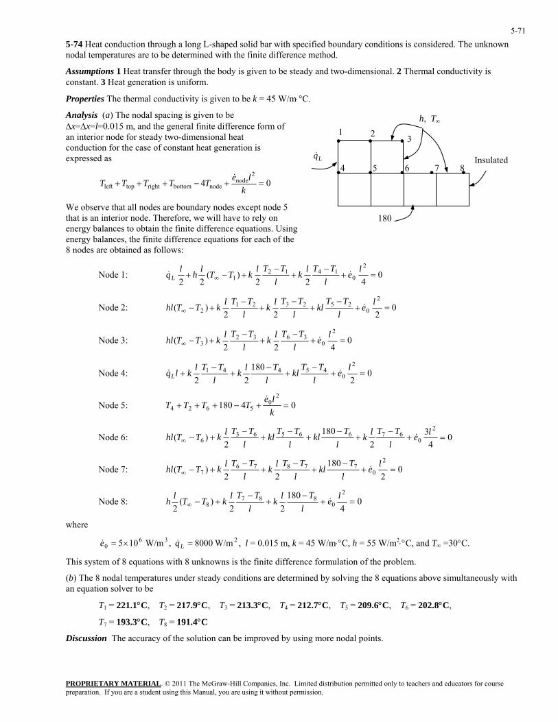
PROPRIETARY MATERIAL. © 2011 The McGraw-Hill Companies, Inc. Limited distribution permitted only to teachers and educators for course preparation. If you are a student using this Manual, you are using it without permission.
5-71
5-74 Heat conduction through a long L-shaped solid bar with specified boundary conditions is considered. The unknown nodal temperatures are to be determined with the finite difference method.
Assumptions 1 Heat transfer through the body is given to be steady and two-dimensional. 2 Thermal conductivity is constant. 3 Heat generation is uniform.
Properties The thermal conductivity is given to be k = 45 W/m⋅°C.
Analysis (a) The nodal spacing is given to be ∆x=∆x=l=0.015 m, and the general finite difference form of an interior node for steady two-dimensional heat conduction for the case of constant heat generation is expressed as
• • •
180
31 2
4 5 6 7 8• • • • •
h, T∞
InsulatedLq&
042
nodenodebottomrighttopleft =+−+++
kleTTTTT
&
We observe that all nodes are boundary nodes except node 5 that is an interior node. Therefore, we will have to rely on energy balances to obtain the finite difference equations. Using energy balances, the finite difference equations for each of the 8 nodes are obtained as follows:
Node 1: 0422
)(22
2
01412
1 =+−
+−
+−+ ∞le
lTTlk
lTTlkTTlhlqL &&
0222
)(2
0252321
2 =+−
+−
+−
+−∞le
lTT
kll
TTlkl
TTlkTThl & Node 2:
0422
)(2
03632
3 =+−
+−
+−∞le
lTTlk
lTTlkTThl & Node 3:
02
18022
2
045441 =+
−+
−+
−+
lel
TTkl
lTlk
lTTlkNode 4: lqL &&
Node 5: 041802
05624 =+−+++
kle
TTTT&
04
32
1802
)(2
06766563
6 =+−
+−
+−
+−
+−∞le
lTTlkNode 6:
lT
kll
TTkl
lTTlkTThl &
Node 7: 02
18022
)(2
077876
7 =+−
+−
+−
+−∞le
lT
kll
TTlkl
TTlkTThl &
Node 8: 04
18022
)(2 0
8878 =+
−+
−+−∞
lel
Tlkl
TTlkTTlh & 2
.
This sys wns is the finite difference formulation of the problem.
ations above simultaneously with an equation solver to be
T1 = 221.1°C, T2 = 217.9°C, T3 = 213.3°C, T4 = 212.7°C, T5 = 209.6°C, T6 = 202.8°C,
T7 = 193.3°C, T8 = 191.4°C
Discussion The accuracy of the solution can be improved by using more nodal points.
where
, W/m8000 , W/m105 2360 =×= Lqe && l = 0.015 m, k = 45 W/m⋅°C, h = 55 W/m2⋅°C, and T∞ =30°C
tem of 8 equations with 8 unkno
(b) The 8 nodal temperatures under steady conditions are determined by solving the 8 equ
PROPRIETARY MATERIAL. © 2011 The McGraw-Hill Companies, Inc. Limited distribution permitted only to teachers and educators for course preparation. If you are a student using this Manual, you are using it without permission.
5-72
Transient Heat Conduction
5-75C The formulation of a transient heat conduction problem differs from that of a steady heat conduction problem in that the transient problem involves an additional term that represents the change in the energy content of the medium with time. This additional term represent the change in the internal energy content during ∆t in the transient finite difference formulation.
tTTxcA im
imp ∆−∆ + /)( 1ρ
5-76C The two basic methods of solution of transient problems based on finite differencing are the explicit and the implicit methods. The heat transfer terms are expressed at time step i in the explicit method, and at the future time step i + 1 in the implicit method as
Explicit method: t
TTcEQ
im
im
pi
∆−
=++
∑1
elementi
element gen,sides All
Vρ&&
tTT
cEQi
mi
mp
i
∆−
=++
+∑1
element1+i
element gen,sides All
1 Vρ&& Implicit method:
5-77C The explicit finite difference formulation of a general interior node for transient heat conduction in a plane wall is
given by τ
im
im
imi
mi
mi
mTT
kxe
TTT−
=∆
++−+
+−
12
11 2&
. The finite difference formulation for the steady case is obtained by
mply setting and disregarding the time index i. It yields im
im TT =+1si
022
11 =++− +− kTTT mmm
∆xem&
5-78C For transient one-dimensional heat conduction in a plane wall with both sides of the wall at specified temperatures, e stability criteria for the explicit method can be expressed in its simplest form as
th
2)( 2∆x
1≤
∆=
tατ
licit method can be expressed in its simplest form as
5-79C For transient one-dimensional heat conduction in a plane wall with specified heat flux on both sides, the stability criteria for the exp
21
)( 2≤
∆
∆=
xtατ
which is identical to the one for the interior nodes. This is because the heat flux boundary conditions have no effect on the stability criteria.
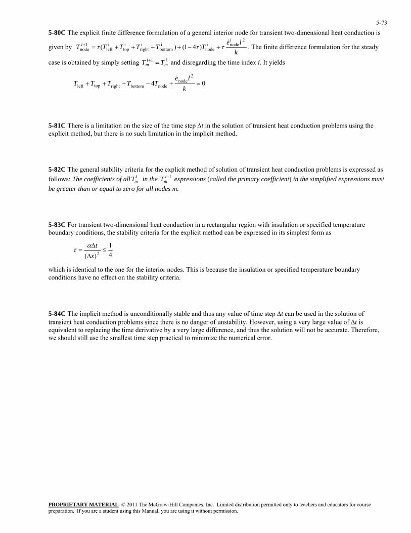
PROPRIETARY MATERIAL. © 2011 The McGraw-Hill Companies, Inc. Limited distribution permitted only to teachers and educators for course preparation. If you are a student using this Manual, you are using it without permission.
5-73
5-80C The explicit finite difference formulation of a general interior node for transient two-dimensional heat conduction is
given by k
leTTTTTT i
2inodei
nodei
bottomi
righti
topi
left1
node )41()(&
τττ +−++++=+ . The finite difference formulation for the steady
case is obtained by simply setting im
im T=+1 and disregarding the time index i. ItT yields
042
nodenodebottomrighttopleft =+−+++
kle
TTTTT&
5-81C There is a limitation on the size of the time step ∆t in the solution of transient heat conduction problems using the explicit method, but there is no such limitation in the implicit method.
5-82C The general stability criteria for the explicit method of solution of transient heat conduction problems is expressed as follows: The coefficients of all i
m in the 1 expressions (called the primary coefficient) in the simplified expressions must be greater than or equal to zero for all nodes m.
T +imT
5-83C For transient two-dimensional heat conduction in a rectangular region with insulation or specified temperature boundary conditions, the stability criteria for the explicit method can be expressed in its simplest form as
4)( 2∆x
interior nodes. This is because the in
1≤
∆tατ
sulation or specified temperature boundary onditions have no effect on the stability criteria.
we should still use the smallest time step practical to minimize the numerical error.
=
which is identical to the one for the c
5-84C The implicit method is unconditionally stable and thus any value of time step ∆t can be used in the solution of transient heat conduction problems since there is no danger of unstability. However, using a very large value of ∆t is equivalent to replacing the time derivative by a very large difference, and thus the solution will not be accurate. Therefore,
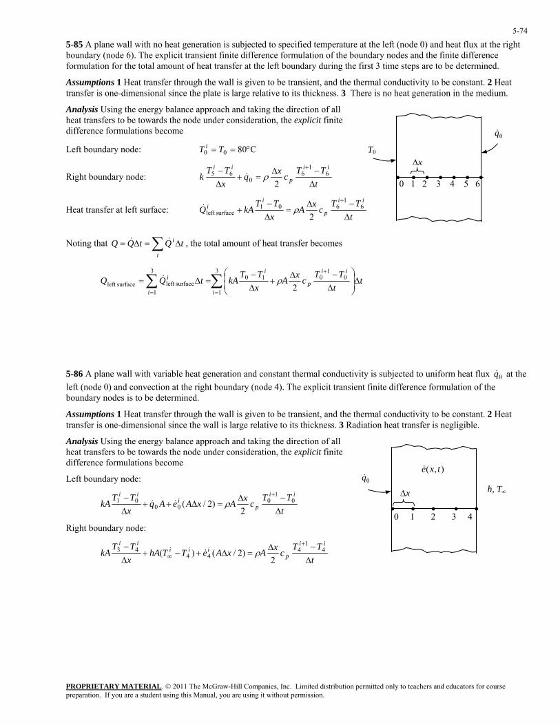
PROPRIETARY MATERIAL. © 2011 The McGraw-Hill Companies, Inc. Limited distribution permitted only to teachers and educators for course preparation. If you are a student using this Manual, you are using it without permission.
5-74
5-85 A plane wall with no heat generation is subjected to specified temperature at the left (node 0) and heat flux at the right boundary (node 6). The explicit transient finite difference formulation of the boundary nodes and the finite difference formulation for the total amount of heat transfer at the left boundary during the first 3 time steps are to be determined.
Assumptions 1 Heat transfer through the wall is given to be transient, and the thermal conductivity to be constant. 2 Heat transfer is one-dimensional since the plate is large relative to its thickness. 3 There is no heat generation in the medium.
Analysis Using the energy balance approach and taking the direction of all heat transfers to be towards the node under consideration, the explicit finite difference formulations become
Left boundary node: C8000 °== TT i
Right boundary node: t
TTcxq
xTT
kii
p
ii
∆−∆
=+∆− +
61
60
65
2ρ&
Heat transfer at left surface: t
TTcxA
x∆surfaceleft TT
kAQii
p
ii
∆−∆
=−
++
61
601
2ρ&
Noting that , the total amount of heat transfer becomes ∑ ∆=∆=i
i tQtQQ &&
∆x T0
• • • • • • • 0 1 2 3 4 5 6
0q&
∑∑=
+
=
∆⎟⎟⎠
⎞⎜⎜⎝
⎛
∆−∆
+∆−
=∆=3
1
01
0103
1surfaceleft surfaceleft 2i
ii
p
i
i
i tt
TTcxA
xTT
kAtQQ ρ&
5-86 A plane wall with variable heat generation and constant thermal conductivity is subjected to uniform heat flux 0q& at left (node 0) and convection at the right boundary (node 4). The explicit transient finite difference formulation of the boundary nodes is to be determined.
the
e thermal conductivity to be constant. 2 Heat Radiation heat transfer is negligible.
y lance approach and taking the direction of all explicit finite
rence formulations become
Left boundary node:
Assumptions 1 Heat transfer through the wall is given to be transient, and thtransfer is one-dimensional since the wall is large relative to its thickness. 3
Analysis Using the energ baheat transfers to be towards the node under consideration, the
h, T∞∆x
• • • • • 0 1 2 3 4
0q&
),( txe&diffe
tTT
cxAxAeAqxTT ii − 01 kA
ii
pi
∆−∆
=∆++∆
+0
10
00 2)2/( ρ&&
Right boundary node:
t
TTcxAxAeTThA
xTT
kAii
piii
ii
∆−∆
=∆+−+∆− +
∞4
14
4443
2)2/()( ρ&
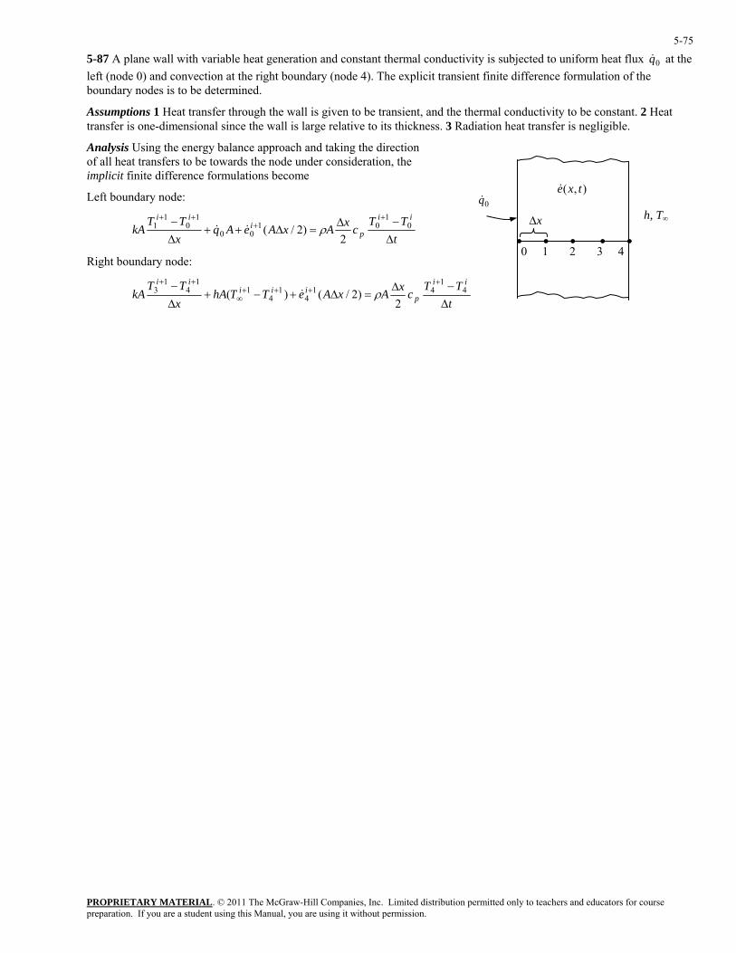
PROPRIETARY MATERIAL. © 2011 The McGraw-Hill Companies, Inc. Limited distribution permitted only to teachers and educators for course preparation. If you are a student using this Manual, you are using it without permission.
5-75
5-87 A plane wall with variable heat generation and constant thermal conductivity is subjected to uniform heat flux at the left (node 0) and convection at the right boundary (node 4). The explicit transient finite difference formulation of the boundary nodes is to be determined.
0q&
Assumptions 1 Heat transfer through the wall is given to be transient, and the thermal conductivity to be constant. 2 Heat transfer is one-dimensional since the wall is large relative to its thickness. 3 Radiation heat transfer is negligible.
Analysis Using the energy balance approach and taking the direction of all heat transfers to be towards the node under consideration, the implicit finite difference formulations become
Left boundary node:
t
TTcxAxAeAq
x∆TT
kAii
pi
ii
∆−∆
=∆++− +
+++
01
0100
10
11
2)2/( ρ&&
Right boundary node:
t
TTcxAxAeTThA
xTT
kAii
piii
ii
∆−∆
=∆+−+∆− +
+++∞
++4
141
41
41
14
13
2)2/()( ρ&
h, T∞∆x
• • • • • 0 1 2 3 4
),( txe&0q&
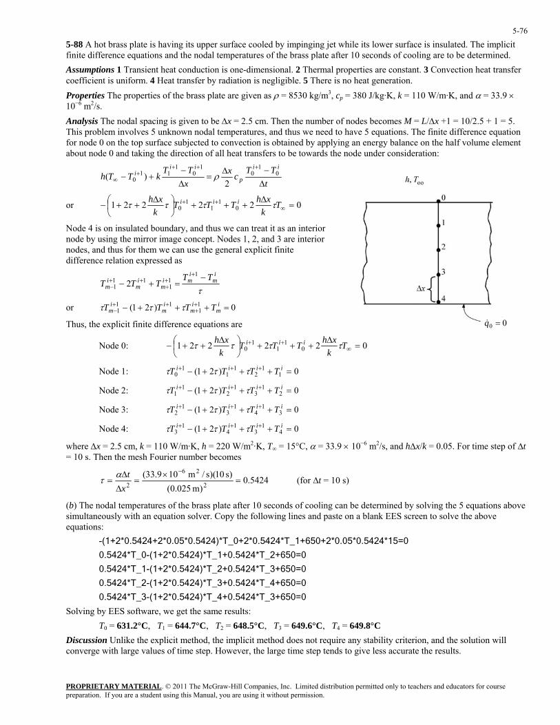
PROPRIETARY MATERIAL. © 2011 The McGraw-Hill Companies, Inc. Limited distribution permitted only to teachers and educators for course preparation. If you are a student using this Manual, you are using it without permission.
5-76
5-88 A hot brass plate is having its upper surface cooled by impinging jet while its lower surface is insulated. The implicit finite difference equations and the nodal temperatures of the brass plate after 10 seconds of cooling are to be determined. Assumptions 1 Transient heat conduction is one-dimensional. 2 Thermal properties are constant. 3 Convection heat transfer coefficient is uniform. 4 Heat transfer by radiation is negligible. 5 There is no heat generation. Properties The properties of the brass plate are given as ρ = 8530 kg/m3, cp = 380 J/kg·K, k = 110 W/m·K, and α = 33.9 × 10⁻⁶ m2/s. Analysis The nodal spacing is given to be ∆x = 2.5 cm. Then the number of nodes becomes M = L/∆x +1 = 10/2.5 + 1 = 5. This problem involves 5 unknown nodal temperatures, and thus we need to have 5 equations. The finite difference equation for node 0 on the top surface subjected to convection is obtained by applying an energy balance on the half volume element about node 0 and taking the direction of all heat transfers to be towards the node under consideration:
t
TTcx
xTT
kTThii
p
iii
∆−∆
=∆−
+−+++
+∞
01
01
01
110 2
)( ρ
00 =q&
022221or 010⎠⎝
∞kk
Node 4 is on insulated boundary, and thus we can treat it as an interior node by using the mirror image concept. Nodes 1, 2, and 3 are inodes, and thus for them we can
11 =∆
+++⎟⎞
⎜⎛ ∆
++− ++ TxhTTTxh iii ττττ
nterior use the general explicit finite
ifference lation expressed as d re
τ11 +++ iii
im
imi
mi
mi
mTT
TTT−
=+−+
++
++−
111
111 2
r 1 =++ +o 1(11 +− 0)2− mmm TTT ττ
hus, the nite difference equations are
imTτ
T explicit fi
022221 01
11
0 =∆
+++⎟⎠⎞
⎜⎝⎛ Node 0: ∆
++− ∞++ T
kxhTTT
kxh iii ττττ
111 =+++− +++ iii TTT τττ
34 =+ TTτ
Node 4: 13
14
13 ++− +++ iii TTT τττ
where ∆x = 2.5 cm, k = 110 W/m·K, h = 220 W/m2·K, T∞ = 15°C, α = 33.9 × 10⁻⁶ m2/s, and h∆x/k = 0.05. For time step of ∆t
Node 1: 0)21( 11
21
11
0 =+++− +++ iiii TTTT τττ
iNode 2: 2321 T
Node 3: )21( 113
12 ++− +++ iiii TT ττ
0)21(
0
04 =+ iT )21(
= 10 s. Then the mesh Fourier number becomes
5424.0)m 025.0(∆x
)s 10)(s/m 109.33( 26×∆ −tατ 22 === (for ∆t = 10 s)
n be determined by solving the 5 equations above
05*0.5424*15=0
*T_3+650=0
T0 = 631.2°C, T1 = 644.7°C, T2 = 648.5°C, T3 = 649.6°C, T4 = 649.8°C Discussion Unlike the explicit method, the implicit method does not require any stability criterion, and the solution will converge with large values of time step. However, the large time step tends to give less accurate the results.
(b) The nodal temperatures of the brass plate after 10 seconds of cooling casimultaneously with an equation solver. Copy the following lines and paste on a blank EES screen to solve the above equations: -(1+2*0.5424+2*0.05*0.5424)*T_0+2*0.5424*T_1+650+2*0.
0.5424*T_0-(1+2*0.5424)*T_1+0.5424*T_2+650=0
0.5424*T_1-(1+2*0.5424)*T_2+0.5424
0.5424*T_2-(1+2*0.5424)*T_3+0.5424*T_4+650=0
0.5424*T_3-(1+2*0.5424)*T_4+0.5424*T_3+650=0
Solving by EES software, we get the same results:
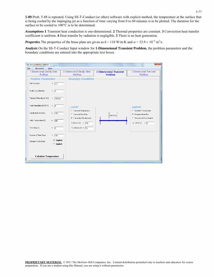
PROPRIETARY MATERIAL. © 2011 The McGraw-Hill Companies, Inc. Limited distribution permitted only to teachers and educators for course preparation. If you are a student using this Manual, you are using it without permission.
5-77
5-89 Prob. 5-88 is repeated. Using SS-T-Conduct (or other) software with explicit method, the temperature at the surface that is being cooled by the impinging jet as a function of time varying from 0 to 60 minutes is to be plotted. The duration for the surface to be cooled to 100°C is to be determined.
Assumptions 1 Transient heat conduction is one-dimensional. 2 Thermal properties are constant. 3 Convection heat transfer coefficient is uniform. 4 Heat transfer by radiation is negligible. 5 There is no heat generation.
Properties The properties of the brass plate are given as k = 110 W/m·K and α = 33.9 × 10⁻⁶ m2/s.
Analysis On the SS-T-Conduct Input window for 1-Dimensional Transient Problem, the problem parameters and the boundary conditions are entered into the appropriate text boxes.
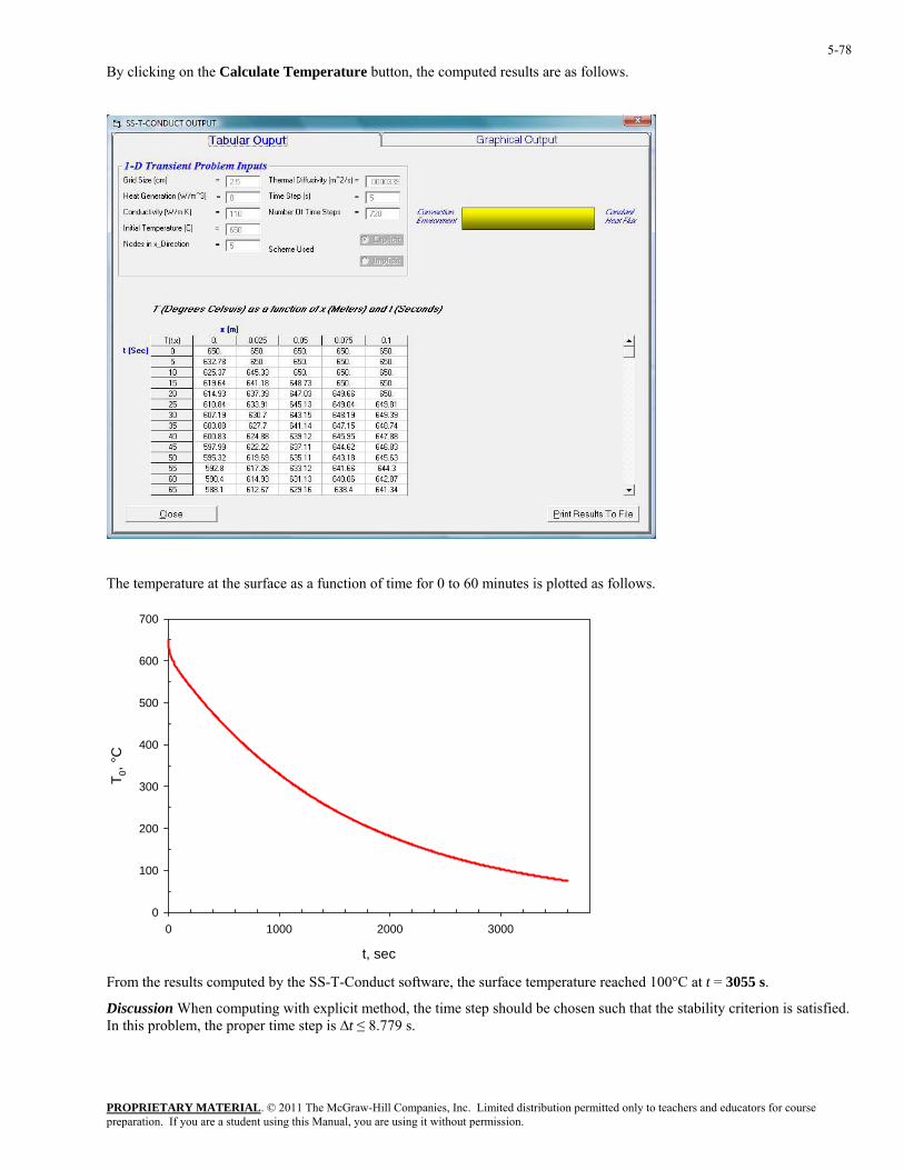
PROPRIETARY MATERIAL. © 2011 The McGraw-Hill Companies, Inc. Limited distribution permitted only to teachers and educators for course preparation. If you are a student using this Manual, you are using it without permission.
5-78
By clicking on the Calculate Temperature button, the computed results are as follows.
The temperature at the surface as a function of time for 0 to 60 minutes is plotted as follows.
t, sec
0 1000 2000 3000
T 0, °C
0
100
200
300
400
500
600
700
From the results computed by the SS-T-Conduct software, the surface temperature reached 100°C at t = 3055 s.
Discussion When computing with explicit method, the time step should be chosen such that the stability criterion is satisfied. In this problem, the proper time step is ∆t ≤ 8.779 s.
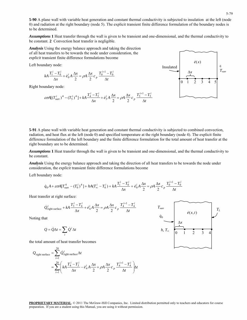
PROPRIETARY MATERIAL. © 2011 The McGraw-Hill Companies, Inc. Limited distribution permitted only to teachers and educators for course preparation. If you are a student using this Manual, you are using it without permission.
5-79
5-90 A plane wall with variable heat generation and constant thermal conductivity is subjected to insulation at the left (node 0) and radiation at the right boundary (node 5). The explicit transient finite difference formulation of the boundary nodes is to be determined.
Assumptions 1 Heat transfer through the wall is given to be transient and one-dimensional, and the thermal conductivity to be constant. 2 Convection heat transfer is negligible.
Analysis Using the energy balance approach and taking the direction of all heat transfers to be towards the node under consideration, the explicit transient finite difference formulations become
Left boundary node:
t
TTcxAxAe
xTT
kAii
pi
ii
∆−∆
=∆
+∆− +
01
00
01
22ρ&
Right boundary node:
t
TTcxAxAe
xTT
kATTAii
pi
iii
∆−∆
=∆
+∆−
+−+
51
55
5445
4isurr 22
])()[( ρεσ &
ary and the finite difference formulation for the total amount of heat transfer at the
1 Heat transfer through the wall is given to be transient and one-dimensional, and the thermal conductivity to
heat transfers to be towards the node under it transient finite difference formulations become
Left boundary node:
∆x
)(xe&
• • • • • •0 1 2 3 4 5
Insulated ε Tsurr
5-91 A plane wall with variable heat generation and constant thermal conductivity is subjected to combined convection, radiation, and heat flux at the left (node 0) and specified temperature at the right boundary (node 4). The explicit finite difference formulation of the left boundright boundary are to be determined.
Assumptions be constant.
Analysis Using the energy balance approach and taking the direction of allconsideration, the explic
tTT
cxAxAexTT
kATThATTAAqii
pi
iiiii
∆−∆
=∆
+∆−
+−+−++
∞0
10
001
04
0surr04
22)(])([ ρεσ &&
t transf at right surface: Hea er
h, T∞
∆x
• • • • • 0 1 2 3 4
Tsurr TL),( txe&
0q&t
TTcxAxAe
xTT
kAQiright &
ii
pi
ii
∆−∆
=∆
+∆−
++
41
44
43surface 22
ρ&
Noting that
the total amount of heat transfer becomes
∑ ∆=∆= i tQtQQ && i
∑
∑
=
+
=
∆⎟⎟⎠
⎞⎜⎜⎝
⎛
∆−∆
+∆
−∆−
=
∆=
20
1
41
44
34
20
1surfaceright surfaceright
22i
ii
pi
iii
i
tt
TTcxAxAe
xTT
kA
tQQ
ρ&
&
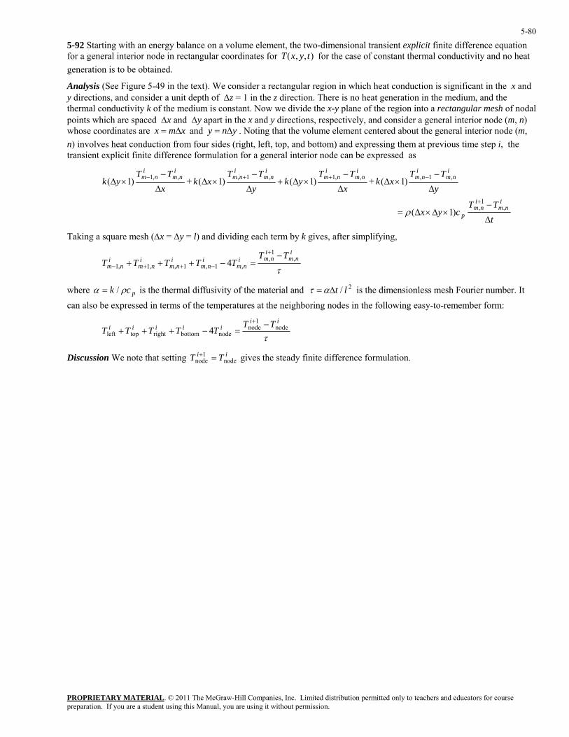
PROPRIETARY MATERIAL. © 2011 The McGraw-Hill Companies, Inc. Limited distribution permitted only to teachers and educators for course preparation. If you are a student using this Manual, you are using it without permission.
5-80
x and (m, e
5-92 Starting with an energy balance on a volume element, the two-dimensional transient explicit finite difference equation for a general interior node in rectangular coordinates for for the case of constant thermal conductivity and no heat generation is to be obtained.
T x y t( , , )
Analysis (See Figure 5-49 in the text). We consider a rectangular region in which heat conduction is significant in the x and y directions, and consider a unit depth of ∆z = 1 in the z direction. There is no heat generation in the medium, and the thermal conductivity k of the medium is constant. Now we divide the x-y plane of the region into a rectangular mesh of nodal points which are spaced ∆x and ∆y apart in the x and y directions, respectively, and consider a general interior node (m, n) whose coordinates are m∆= yn∆= . Noting that the volume element centered about the general interior node n) involves heat conduction from four sides (right, left, top, and bottom) and expressing them at previous time step i, thtransient explicit finite difference formulation for a general interior node can be expressed as
x y
tTT
cyx
yTT
xkxyx ∆∆∆
TTyk
TTxk
TTyk
inm
inm
p
inm
inm
inm
inm
inm
inm
inm
inm
∆
−×∆×∆=
∆
−×∆
−×∆+
−×∆
−×
+
−++−
,1
,
,1,,,1,1,,,1
)1(
)1(+)1()1(+)1
ρ
Taking a square mesh (∆x = ∆y = l) and dividing each term by k gives, after simplifying,
∆(
τ
inm
inmi
nmi
nmi
nmi
nmi
nmTT
TTTTT ,1
,4−
=−++++
−++− ,1,1,,1,1
where pck ρα /= is the thermal diffusivity f the material and 2/ lt∆=ατ is the dimension o less mesh Fourier number. It can also be expressed in terms of the temperatures at the neighboring nodes in the following easy-to-remember form:
τ
iiiiiii TT
TTTTT node1
nodenodebottomrighttopleft 4
−=−+++
+
Discussion We note that setting gives the steady finite difference formulation. ii TT node1
node =+
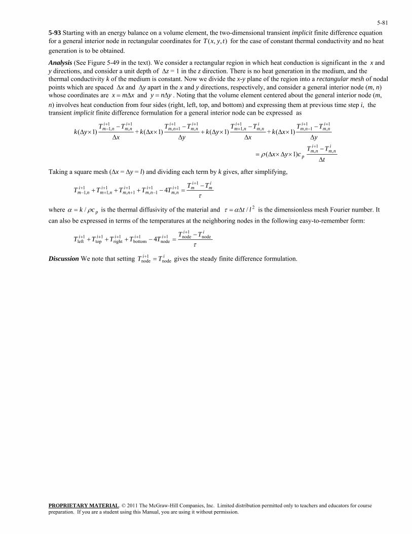
PROPRIETARY MATERIAL. © 2011 The McGraw-Hill Companies, Inc. Limited distribution permitted only to teachers and educators for course preparation. If you are a student using this Manual, you are using it without permission.
5-81
o heat
m, e
5-93 Starting with an energy balance on a volume element, the two-dimensional transient implicit finite difference equation for a general interior node in rectangular coordinates for ),,( tyx for the case of constant thermal conductivity and ngeneration is to be obtained.
T
Analysis (See Figure 5-49 in the text). We consider a rectangular region in which heat conduction is significant in the x and y directions, and consider a unit depth of ∆z = 1 in the z direction. There is no heat generation in the medium, and the thermal conductivity k of the medium is constant. Now we divide the x-y plane of the region into a rectangular mesh of nodal points which are spaced ∆x and ∆y apart in the x and y directions, respectively, and consider a general interior node (m, n) whose coordinates are and yn∆= . Noting that the volume element centered about the general interior node (n) involves heat conduction from four sides (right, left, top, and bottom) and expressing them at previous time step i, thtransient implicit finite difference formulation for a general interior node can be expressed as
xmx ∆= y
tTT
cyx
yTT
xkx
TTyk
yTT
xkx
TTyk
inm
inm
p
inm
inm
inm
inm
inm
inm
inm
inm
∆
−×∆×∆=
∆
−×∆
∆
−×∆+
∆
−×∆
∆
−×∆
+
++−
++
+++
++−
,1
,
1,
11,,
1,1
1,
11,
1,
1,1
)1(
)1(+ )1()1(+)1(
ρ
Taking a square mesh (∆x = ∆y = l) and dividing each term by k gives, after simplifying,
τnmnmnmnm −+
im
imiiii
nmTT
TTTTT−
=−++++
++++i++−
111111
,1 4
urier number. It can also be expressed in terms of the temperatures at the neighboring nodes in the following easy-to-remember form:
,1,1,,1
where pck ρα /= is the thermal diffusivity of the material and 2/ lt∆=ατ is the dimensionless mesh Fo
τnodebottomrighttopleft
iiiiiii TT
TTTTT node1
node11111 4−
=−++++
+++++
iscussion We note that setting gives the steady finite difference formulation.
ii TT node1
node =+D
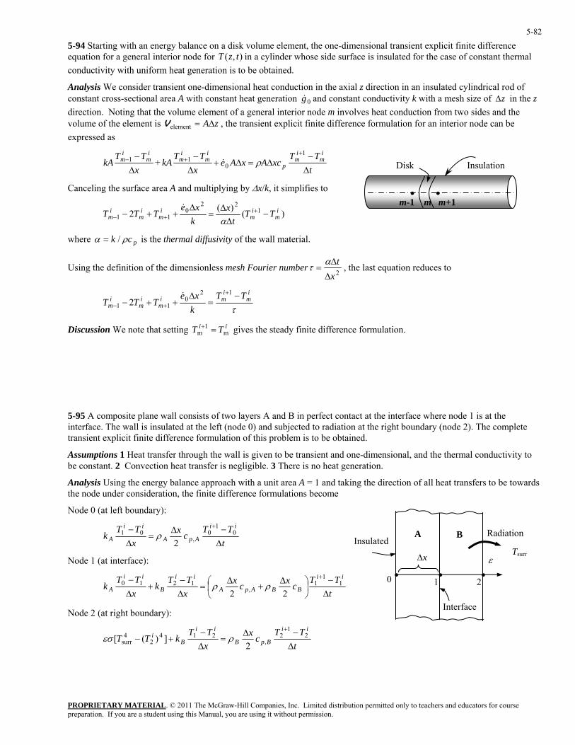
PROPRIETARY MATERIAL. © 2011 The McGraw-Hill Companies, Inc. Limited distribution permitted only to teachers and educators for course preparation. If you are a student using this Manual, you are using it without permission.
5-82
5-94 Starting with an energy balance on a disk volume element, the one-dimensional transient explicit finite difference equation for a general interior node for in a cylinder whose side surface is insulated for the case of constant thermal conductivity with uniform heat generation is to be obtained.
),( tzT
Analysis We consider transient one-dimensional heat conduction in the axial z direction in an insulated cylindrical rod of constant cross-sectional area A with constant heat generation 0 and constant conductivity k with a mesh size ofg& z∆ in the zdirection. Noting that the volume element of a general interior node m involves heat conduction from two sides and the volume of the element is zA∆=element , the transient explicit finite difference formulation for an interior node can be
expressed as V
txx ∆∆∆TT
xcAxAeTT
kATT
kAi
mi
mp
im
im
im
im −
∆=∆+−− +
+−1
011 + ρ&
Canceling the surface area A and multiplying by ∆x/k, it simplifies to
)()( 122
01
im
im
im
im TTxxe
T −∆
=∆
++ ++
& 21
im tk
TT∆
−− α
Using the definition of the dimensionless mesh Fourier number
where pck ρα /= is the thermal diffusivity of the wall material.
2xt
∆
∆=ατ , the last equation reduces to
τ
ii −+12mmi
mi
mi
mTT
kxe
TTT =∆
++− +−0
11 2&
We note that setting gives the steady finite difference formulation.
ght boundary (node 2). The complete
one-dimensional, and the thermal conductivity to t tran s negligible. 3 There is no heat generation.
Analysis Using the energy balance approach with a unit area A = 1 and taking the direction of all heat transfers to be towards the node under consideration, the finite difference formulations become
Discussion ii TT m1
m =+
5-95 A composite plane wall consists of two layers A and B in perfect contact at the interface where node 1 is at the interface. The wall is insulated at the left (node 0) and subjected to radiation at the ritransient explicit finite difference formulation of this problem is to be obtained.
Assumptions 1 Heat transfer through the wall is given to be transient and
• • m-1 m m+1
InsulationDisk
Insulated
∆x
1
ε• ••0 2
A
Tsurr
RadiationB
Interface
be constant. 2 Convection hea sfer i
Node 0 (at left boundary):
tTT
cxx 2TT
kii
ApA
ii
∆−∆
=∆− +
01
0,
01 ρ
Node 1 (at interface):
A
tTT
cxcxxTT
kxTT
kii
1BBApA
ii
B
ii
A ∆−
⎟⎠⎞
⎜⎝⎛ ∆
+∆
=∆−
+∆− +
11
,1210
22ρρ
Node 2 (at right boundary):
tTT
cxxTT
kTTii
BpB
ii
Bi
∆−∆
=∆−
+−+
21
2,
2142
4surr 2
])([ ρεσ
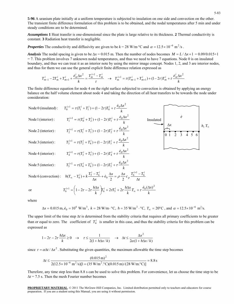
PROPRIETARY MATERIAL. © 2011 The McGraw-Hill Companies, Inc. Limited distribution permitted only to teachers and educators for course preparation. If you are a student using this Manual, you are using it without permission.
5-83
α .
5-96 A uranium plate initially at a uniform temperature is subjected to insulation on one side and convection on the other. The transient finite difference formulation of this problem is to be obtained, and the nodal temperatures after 5 min and under steady conditions are to be determined.
Assumptions 1 Heat transfer is one-dimensional since the plate is large relative to its thickness. 2 Thermal conductivity is constant. 3 Radiation heat transfer is negligible.
Properties The conductivity and diffusivity are given to be k = 28 W/m⋅°C and = /sm 105.12 26−×
Analysis The nodal spacing is given to be ∆x = 0.015 m. Then the number of nodes becomes 1/ +∆= xLM = 0.09/0.015+1 = 7. This problem involves 7 unknown nodal temperatures, and thus we need to have 7 equations. Node 0 is on insulated boundary, and thus we can treat it as an interior note by using the mirror image concept. Nodes 1, 2, and 3 are interior nodes, and thus for them we can use the general explicit finite difference relation expressed as
τ
im
im
imi
mi
mi
mTT
kxe
TT−−1 2T−
=∆
+++
+
12
1&
→ k
xeTTTT
imi
mi
mi
mi
m
2
111 )21()(
∆+−++= +−
+ &τττ
The finite difference equation for node 4 on the right surface subjected to convection is obtained by applying an energy balance on the half volume element about node 4 and taking the direction of all heat transfers to be towards the node under consideration:
tTT
cxxeTT
kTThiiii
i −∆=
∆+
−+−
+6
1665)( :n)(convectioNode ρ&
x
kxe
TTTT
kxe
TTTT
kxe
TT
kxe
TTTT
kxe
TTTT
p
iiii
iiii
iiii
iiii
iiii
∆∆
∆+−++=
∆+−++=
∆+−+=
∆+−++=
∆+−++=
∞
+
+
+
+
+
06
20
5641
5
0453
14
20
231
2
20
1201
1
20
0111
0
22 6
)21()( :(interior) 5 Node
)21()( :r)
)21() :(interior) 2 Node
)21()( :(interior) 1 Node
)21()( :)(insulated 0 Node
τττ
τττ
ττ
τττ
τττ
&
&
&
&
&
or
TT +1(τ
kxe
TTTT iiii ∆+−++=+
2
20
3421
3
(interio 4 Node
)21()( :(interior) 3 Node τττ&
kkk ⎠⎝
where
xeTxhTTxhT iii
20
561
6)(
22221∆
+∆
++⎟⎞
⎜⎛ ∆
−−= ∞+ &
τττττ
& , and m2/s.
er ro. The coefficient of is smaller in this case, and thus the stability criteria for this problem can be
C20 C, W/m35 C, W/m28 , W/m10 m, 015.0 2360 °=°⋅=°⋅===∆ ∞Thke 6105.12 −×=αx
The upper limit of the time step ∆t is determined from the stability criteria that requires all primary coefficients to be greatthan or equal to ze iT4
expressed as
)/1(2
)/1(2
0221kxh
tkxhk ∆+
≤∆→∆+
≤→≥−−α
τττ
since 2/ xt ∆∆=ατ . Substituting the given quantities, the maximum allowable the time step becomes
1 2xxh ∆∆
s 8.8C)] W/m.28/(m) 015.0)(C. W/m35(1/s)[m 105.12(2
)m 015.0( 2
226 =°°+×
≤∆−
t
Therefore, any time step less than 8.8 s can be used to solve this problem. For convenience, let us choose the time step to be ∆t = 7.5 s. Then the mesh Fourier number becomes
h, T∞∆x
Insulated
• • • • • • • 0 1 2 3 4 5 6
e&
PROPRIETARY MATERIAL. © 2011 The McGraw-Hill Companies, Inc. Limited distribution permitted only to teachers and educators for course preparation. If you are a student using this Manual, you are using it without permission.
5-84
4167.0)m 015.0( 22 ==
∆=
xτ s) /s)(7.5m 105.12( 26×∆ −tα
Substituting this value of τ and other given quantities, the nodal temperatures after 5×60/7.5 = 40 time steps (5 min) are ined to be determ
After 5 min:
T = 229.9°C, T = 229.7°C, T = 229.0°C, T = 227.7°C, T = 225.8°C, T = 223.3°C, and T6 = 220.0 °C
the number of time steps until the nodal temperatures no longer change. Using EES, we increased time steps for 16.8 hours (60500 seconds). The temperatures seem to remain constant at about this time. Then, the nodal temperatures under steady conditions are
T0 = 2736°C, T1 = 2732°C, T2 = 2720°C, T4 = 2700°C, T5 = 2672°C, T6 = 2636°C, and T7 = 2591 °C
0 1 2 3 4 5
b) The time needed for transient operation to be established is determined by increasing (
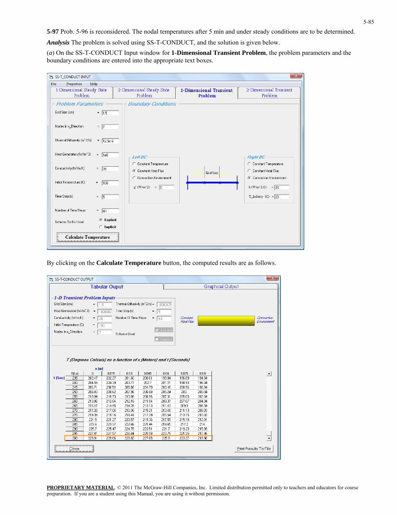
PROPRIETARY MATERIAL. © 2011 The McGraw-Hill Companies, Inc. Limited distribution permitted only to teachers and educators for course preparation. If you are a student using this Manual, you are using it without permission.
5-85
5-97 Prob. 5-96 is reconsidered. The nodal temperatures after 5 min and under steady conditions are to be determined.
ThT Input window for 1-Dimensional Transient Problem, the problem parameters and the
Analysis e problem is solved using SS-T-CONDUCT, and the solution is given below. (a) On the SS-T-CONDUCboundary conditions are entered into the appropriate text boxes.
By clicking on the Calculate Temperature button, the computed results are as follows.
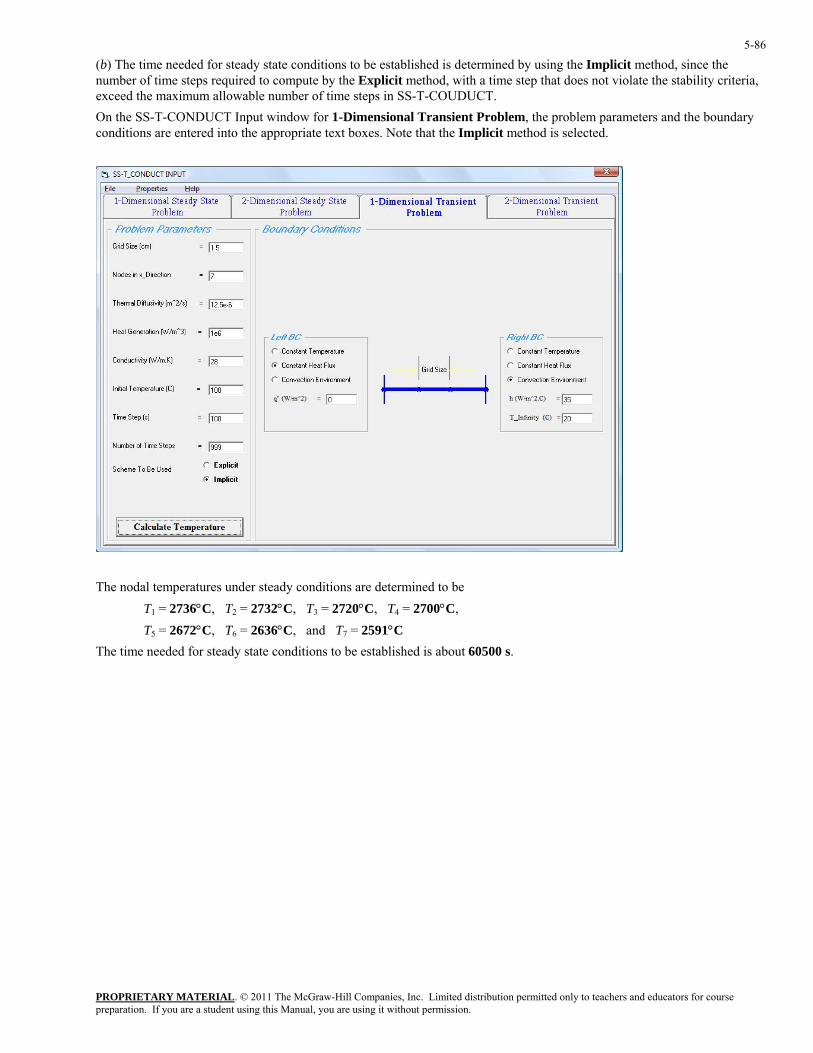
PROPRIETARY MATERIAL. © 2011 The McGraw-Hill Companies, Inc. Limited distribution permitted only to teachers and educators for course preparation. If you are a student using this Manual, you are using it without permission.
5-86
) The time needed for steady state conditions to be established is determined by using the Implicit method, since the number of time steps required to compute by the E cit me , with e st at do violate the stability criteria, exceed the maximu owab mber of time ste SS-T UDUOn the SS-T-COND Inp ow im T m parameters and the boundary condit re ente th ria box e t mp ethod is selected.
(bxpli thod a tim ep th es not
m all le nu ps in -CO CT. UCT
red intout winde approp
for 1-Dte text
ensional ransient Problhat the I
elicit m
, the problemions a es. Not
The nodal temperatures under steady conditions are determined to be
T1 = 2736°C, T2 = 2732°C, T3 = 2720°C, T4 = 2700°C, T5 = 2672°C, T6 = 2636°C, and T7 = 2591°C
The time needed for steady state conditions to be established is about 60500 s.
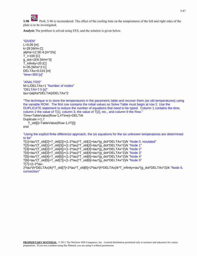
PROPRIETARY MATERIAL. © 2011 The McGraw-Hill Companies, Inc. Limited distribution permitted only to teachers and educators for course preparation. If you are a student using this Manual, you are using it without permission.
5-87
5-98 Prob. 5-96 is reconsidered. The effect of the cooling time on the temperatures of the left and right sides of the plate is to be investigated.
Analysis The problem is solved using EES, and the solution is given below.
g_dot=1E6 [W/m^3] ity=20 [C]
h=35 [W/m^2-C]
M=L/DELTAx+1 "Number of nodes" "DELTAt=7.5 [s]" tau=(alpha*DELTAt)/DELTAx^2 "The technique is to store the temperatures in the parametric table and recover them (as old temperatures) using the variable ROW. The first row contains the initial values so Solve Table must begin at row 2. Use the
UPLICATE statement to reduce the number of equations that need to be typed. Column 1 contains the time, value of T[2], etc., and column 9 the Row."
Time=TableValue(Row-1,#Time)+DELTAt Duplicate i=1,7 T_old[i]=TableValue(Row-1,#T[i]) end
"Using the explicit finite difference approach, the six equations for the six unknown temperatures are determined
tau)*T_old[3]+tau*(g_dot*DELTAx^2)/k "Node 2" tau)*T_old[4]+tau*(g_dot*DELTAx^2)/k "Node 3"
T[5]=tau*(T_old[4]+T_old[6])+(1-2*tau)*T_old[5]+tau*(g_dot*DELTAx^2)/k "Node 4" T[6]=tau*(T_old[5]+T_old[7])+(1-2*tau)*T_old[6]+tau*(g_dot*DELTAx^2)/k "Node 5"
1-2*tau-2*tau*(h*DELTAx)/k)*T_old[7]+2*tau*T_old[6]+2*tau*(h*DELTAx)/k*T_infinity+tau*(g_dot*DELTAx^2)/k "Node 6, convection"
"GIVEN" L=0.09 [m] k=28 [W/m-C] alpha=12.5E-6 [m^2/s] T_i=100 [C]
T_infin
DELTAx=0.015 [m] "time=300 [s]" "ANALYSIS"
Dcolumn 2 the value of T[1], column 3, the
to be" T[1]=tau*(T_old[2]+T_old[2])+(1-2*tau)*T_old[1]+tau*(g_dot*DELTAx^2)/k "Node 0, insulated" T[2]=tau*(T_old[1]+T_old[3])+(1-2*tau)*T_old[2]+tau*(g_dot*DELTAx^2)/k "Node 1" T[3]=tau*(T_old[2]+T_old[4])+(1-2*T[4]=tau*(T_old[3]+T_old[5])+(1-2*
T[7]=(
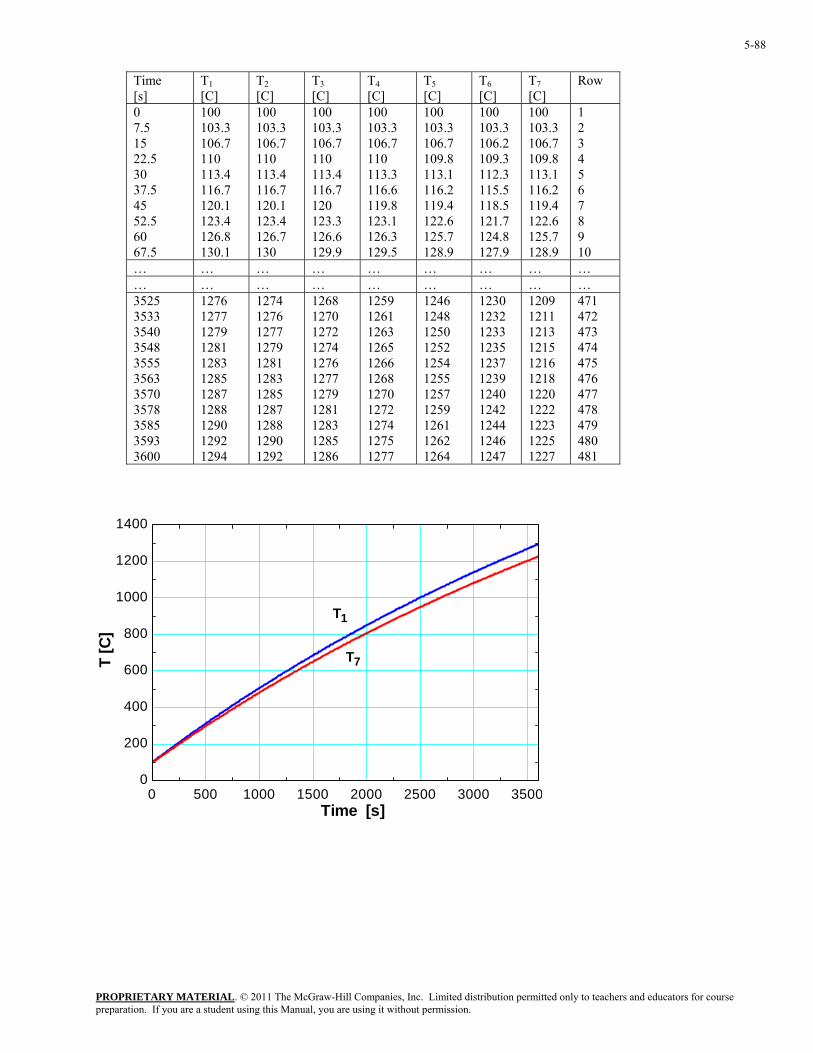
PROPRIETARY MATERIAL. © 2011 The McGraw-Hill Companies, Inc. Limited distribution permitted only to teachers and educators for course preparation. If you are a student using this Manual, you are using it without permission.
5-88
] [C] [C] [C] [C] [C] [C]
Time [s]
T1 [C
T2 T3 T4 T5 T6 T7 Row
0 7.5 15
100 103.3 106.7
100 103.3 106.7
100 103.3 106.7
100 103.3 106.7
100 103.3 106.7
100 103.3 106.2
100 103.3
1 2
22.5 110 110 110 110 130 37.5 45 52.5 60
113.4 116.7 120.1 123.4 126.8
113.4 116.7 120.1 123.4
113.4 116.7 120 123.3
113.3 116.6 119.8 123.1
113.1 116.2 119.4 122.6
112.3 115.5 118.5 121.7
11311611912
67.5 130.1 126.7 130
126.6 129.9
126.3 129.5
09.8
125.7 128.9
109.3
124.8 127.9
106.7 109.8
.1
.2
.4 2.6
125.7 128.9
3 4 5 6 7 8 9 10
… … … … … … … … … … … … … … … … … … 3525 3533 3540 3548 3555 3563 3570 3578 3585 3593 3600
1276 1277 1279 1281 1283 1285 1287 1288 1290 1292 1294
1274 1276 1277 1279 1281 1283 1285 1287 1288 1290 1292
1268 1270 1272 1274 1276 1277 1279 1281 1283 1285 1286
1259 1261 1263 1265 1266 1268 1270 1272 1274 1275 1277
1246 1248 1250 1252 1254 1255 1257 1259 1261 1262 1264
1230 1232 1233 1235 1237 1239 1240 1242 1244 1246 1247
1209 1211 1213 1215 1216 1218 1220 1222 1223 1225 1227
471 472 473 474 475 476 477 478 479 480 481
0 500 1000 1500 2000 2500 3000 35000
200
400
600
800
1000
1200
1400
Time [s]
T [C
]
T1
T7
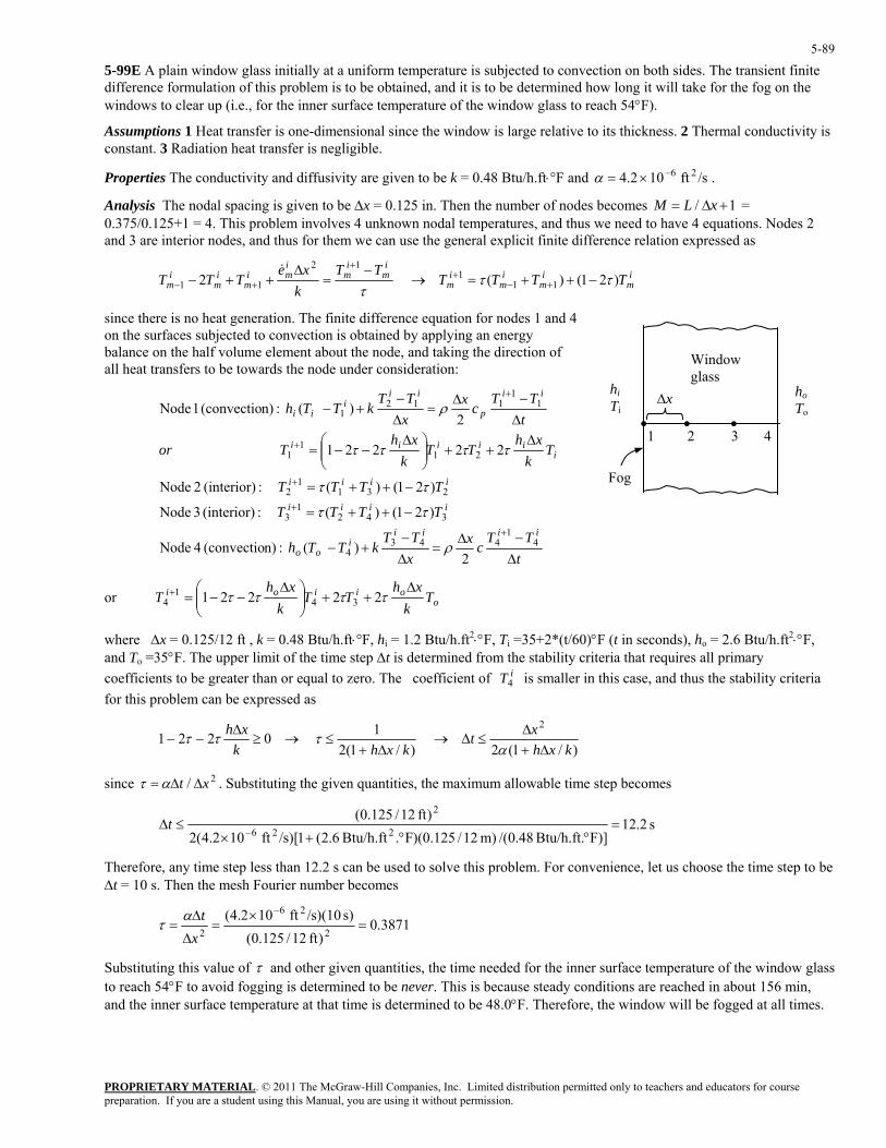
PROPRIETARY MATERIAL. © 2011 The McGraw-Hill Companies, Inc. Limited distribution permitted only to teachers and educators for course preparation. If you are a student using this Manual, you are using it without permission.
5-89
-99E A plain window glass initially at a uniform temperature is subjected to convection on both sides. The transient finite difference formulation of this problem is to be obtained, and it is to be determined how long it will take for the fog on the windows to clear up (i.e., for the inner surface temperature of the window glass to reach 54°F).
ssumptions 1 Heat transfer is one-dimensional since the window is large relative to its thickness. 2 Thermal conductivity is
Properties The conductivity and diffusivity are given to be k = 0.48 Btu/h.ft⋅°F and
lysis The nodal spacing is given to be ∆x = 0.125 in. Then the number of nodes become
5
Aconstant. 3 Radiation heat transfer is negligible.
/sft 102.4 26−×=α .
s 1/ +∆= xLMAna = 0.375/0.125+1 = 4. This problem involves 4 unknown nodal temperatures, and thus we need to have 4 equations. Nodes 2
rior nodes, and t f hem we can use the general explicit finite difference relation expressed as and 3 are inte hus or t
τ
im
im
imiii TTxe
TTT−
=∆
++−+12
2&
→ iiii TTTT )21()(1 ττ −++=+ mmm k+− 11 mmm 11 +−
since there is no heat generation. The fi tion for nodes 1 and 4 on the surfaces subjected to convection balance on the half volume n i ion of all hea f tow ode r tion
m
nite difference equais obtained by aut the
pplying an energy ode, and tak element abo ng the direct
t trans ers to be ards the n unde considera : hoTo
∆x
Fog
• • • 1 2 3 4
Window glass
hiTi
tc
xkTTh oo ∆
=∆
+− 4 2)( :n)(convectio 4 Node ρ
TTxTT
TTT
TT
Tk
xhT
tT
kT
iiiii
ii
ii
iii
i
i
−∆−
−+
∆+⎟⎟
⎠
⎞⎜⎜⎝
⎛=
∆−
=−
+
+
41
443
34
23
1
11
)21()(ior)Nod
)(ior)d
221
ectiod
ττ
ττ
τ
ρ
T i =+13
2
:
Ti +T i =+1 :
T i +22τk
xhiτT i+11 or
Tcx i
p∆ 1
x∆
∆TT ii − 12Thi ( :n)
i2
1
i +1 )
+
−+ 21()
−− 2τ
(inter 3 e
(inter 2 eNo
2(conv 1 eNo
ooiioi Tk
xhTT
kxh
T∆
++⎟⎟⎠
⎞⎜⎜⎝
⎛ ∆−−=+ ττττ 22221 34
14 or
where ∆x = 0.125/12 ft , k = 0.48 Btu/h.ft⋅°F, hi = 1.2 Btu/h.ft2⋅°F, Ti =35+2*(t/60)°F (t in seconds), ho = 2.6 Btu/h.ft2⋅°F, and To =35°F. The upper limit of the time step ∆t is determined from the stability criteria that requires all primary coefficients to be greater than or equal to zero. The coefficient of is smaller in this case, and thus the stability criteria for this problem can be expressed as
iT4
)/1(2
)/1(2
1 02212
kxhxt
kxhkxh
∆+∆
≤∆→∆+
≤→≥∆
−−α
τττ
since . Substituting the given quantities, the maximum allowable time step becomes 2/ xt ∆∆=ατ
s 2.12F)]Btu/h.ft. 48.0/(m) 12/125.0)(F.Btu/h.ft 6.2(1/s)[ft 102.4(2
)ft 12/125.0(226
2=
°°+×≤∆
−t
Therefore, any time step less than 12.2 s can be used to solve this problem. For convenience, let us choose the time step to be ∆t = 10 s. Then the mesh Fourier number becomes
3871.0)ft 12/125.0(
s) /s)(10ft 102.4(2
26
2=
×=
∆
∆=
−
xtατ
τ and other given quantities, the time needed for the inner surface temperature of the window glass Substituting this value ofto reach 54°F to avoid fogging is determined to be never. This is because steady conditions are reached in about 156 min, and the inner surface temperature at that time is determined to be 48.0°F. Therefore, the window will be fogged at all times.
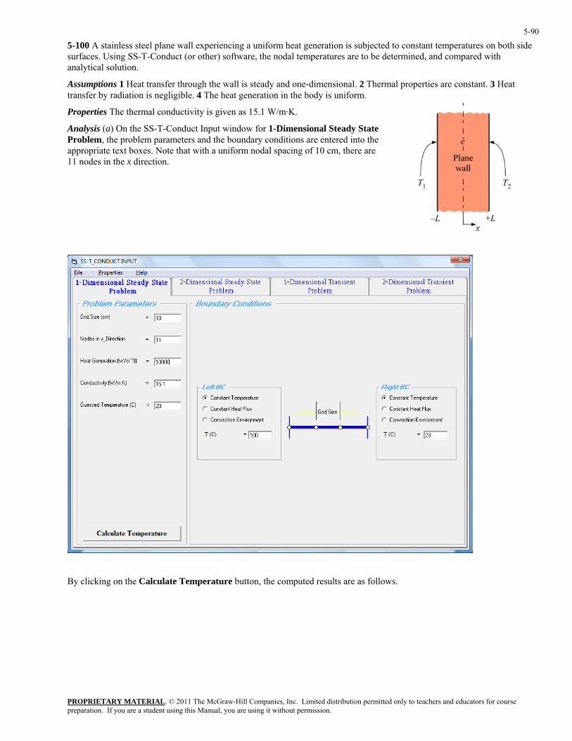
PROPRIETARY MATERIAL. © 2011 The McGraw-Hill Companies, Inc. Limited distribution permitted only to teachers and educators for course preparation. If you are a student using this Manual, you are using it without permission.
5-90
ough the wall is steady and one-dimensional. 2 Thermal properties are constant. 3 Heat
n.
5-100 A stainless steel plane wall experiencing a uniform heat generation is subjected to constant temperatures on both sidesurfaces. Using SS-T-Conduct (or other) software, the nodal temperatures are to be determined, and compared with analytical solution.
Assumptions 1 Heat transfer thrtransfer by radiation is negligible. 4 The heat generation in the body is uniform.
Properties The thermal conductivity is given as 15.1 W/m·K.
Analysis (a) On the SS-T-Conduct Input window for 1-Dimensional Steady State Problem, the problem parameters and the boundary conditions are entered into the appropriate text boxes. Note that with a uniform nodal spacing of 10 cm, there are 11 nodes in the x directio
By clicking on the Calculate Temperature button, the computed results are as follows.
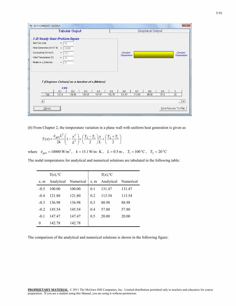
PROPRIETARY MATERIAL. © 2011 The McGraw-Hill Companies, Inc. Limited distribution permitted only to teachers and educators for course preparation. If you are a student using this Manual, you are using it without permission.
5-91
(b) From Chapter 2, the temperature variation in a plane wall with uniform heat generation is given as
⎟⎠
⎞⎜⎝
⎛ ++⎟
⎠
⎞⎜⎝
⎛ −+⎟
⎟⎠
⎞⎜⎜⎝
⎛−=
221
2)( 1212
2
22 TTLxTT
Lx
kLe
xT gen&
where 3 W/m10000= , K W/m1.15 ⋅=k , m 5.0=L , C 100gene& 1 °=T C 202 °=T ,
The nodal temperatures for analytical and numerical solutions are tabulated in the following table:
T(x),°C T(x),°C
x, m Analytical Numerical x, m Analytical Numerical
-0.5 100.00 100.00 0.1 131.47 131.47
-0.4 121.80 121.80 0.2 113.54 113.54
-0.3 136.98 136.98 0.3 88.98 88.98
-0.2 145.54 145.54 0.4 57.80 57.80
-0.1 147.47 147.47 0.5 20.00 20.00
0 142.78 142.78
The comparison of the analytical and numerical solutions is shown in the following figure:
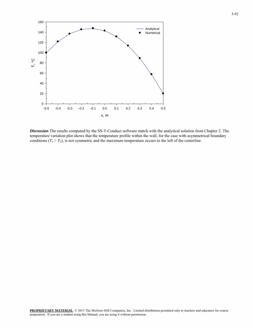
PROPRIETARY MATERIAL. © 2011 The McGraw-Hill Companies, Inc. Limited distribution permitted only to teachers and educators for course preparation. If you are a student using this Manual, you are using it without permission.
5-92
x, m
T, °
160
AnalyticalNumerical140
100
120
C
0
20
40
60
80
-0.5 -0.4 - -0.2 -0.1 0. 0.1 0.2 0.3 0.4 0.50.3 0
iscussion The results computed by the SS-T-Conduct software match with the analytical solution from Chapter 2. The mperature variation plot shows that the temperature profile within the wall, for the case with asymmetrical boundary
onditions (T1 > T2), is not symmetric and the maximum temperature occurs to the left of the centerline.
Dtec
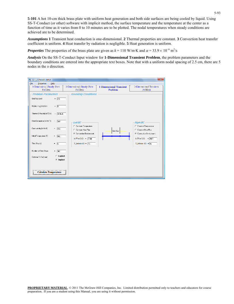
PROPRIETARY MATERIAL. © 2011 The McGraw-Hill Companies, Inc. Limited distribution permitted only to teachers and educators for course preparation. If you are a student using this Manual, you are using it without permission.
5-93
5-101 A hot 10-cm thick brass plate with uniform heat generation and both side surfaces are being cooled by liquid. Using o duct (o ther) software with implicit method, the surface temperature and the temperature at the center as a
function of time as it varies from 0 to 10 minutes are to be plotted. The nodal temperatures when steady conditions are are to be determined.
Assump n ensi are constant. 3 Convection heat transfer coefficient is uniform .
Properties −6 m2/s
SS-T-C n r o
achieved
tions 1 Transient heat conductio is one-dim onal. 2 Thermal properties. 4 Heat transfer by radiation is negligible. 5 Heat generation is uniform
The properties of the brass plate are given as k = 110 W/m·K and α = 33.9 × 10
Analysis On the SS-T-Conduct Input window for 1-Dimensional Transient Problem, the problem parameters and the boundary conditions are entered into the appropriate text boxes. Note that with a uniform nodal spacing of 2.5 cm, there are 5nodes in the x direction.
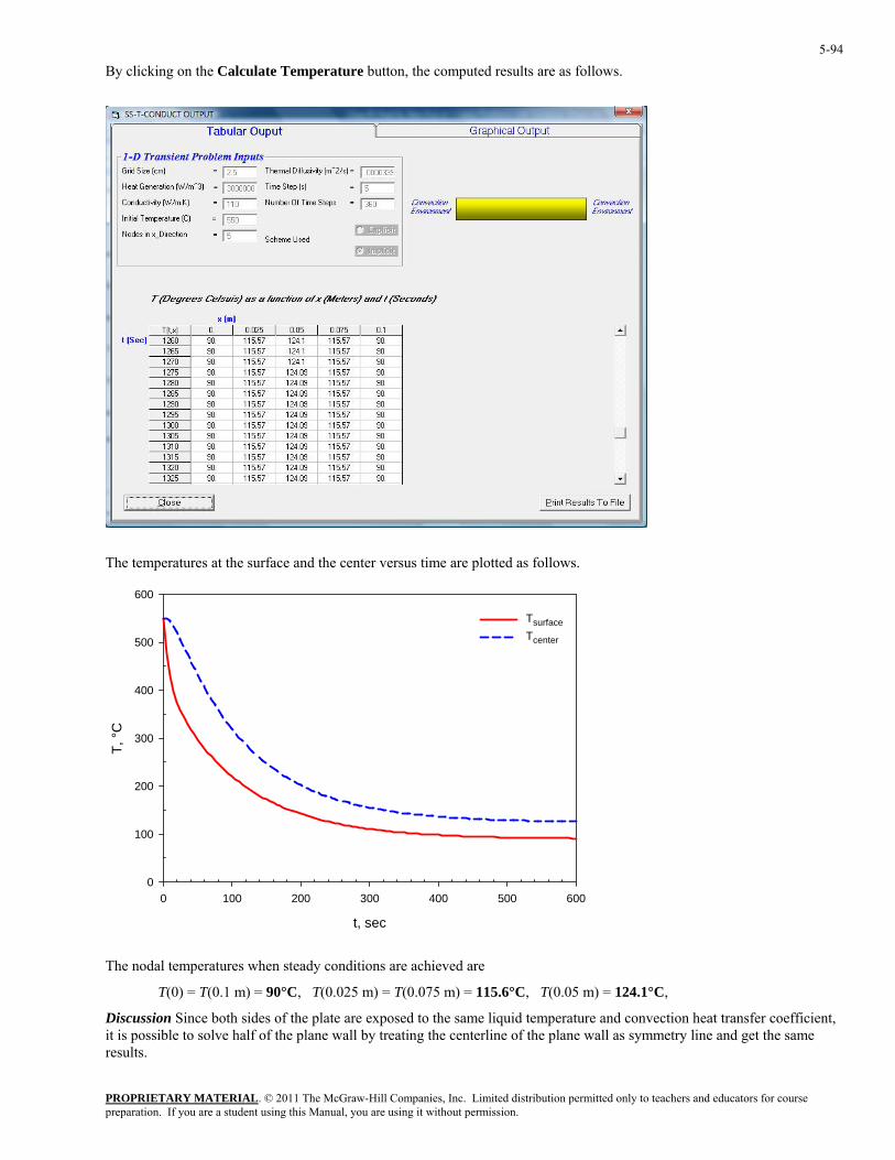
PROPRIETARY MATERIAL. © 2011 The McGraw-Hill Companies, Inc. Limited distribution permitted only to teachers and educators for course preparation. If you are a student using this Manual, you are using it without permission.
5-94
y clicking on the Calculate Temperature button, the computed results are as follows. B
The temperatures at the surface and the center versus time are plotted as follows.
t, sec
0 100 200 300 400 500 600
T, °
C
0
100
200
300
600
500
400
Tsurface Tcenter
Discussion Since both sides of the plate are exposed to the same liquid temperature and convection heat transfer coefficient, it is possible to solve half of the plane wall by treating the centerline of the plane wall as symmetry line and get the same results.
The nodal temperatures when steady conditions are achieved are
T(0) = T(0.1 m) = 90°C, T(0.025 m) = T(0.075 m) = 115.6°C, T(0.05 m) = 124.1°C,
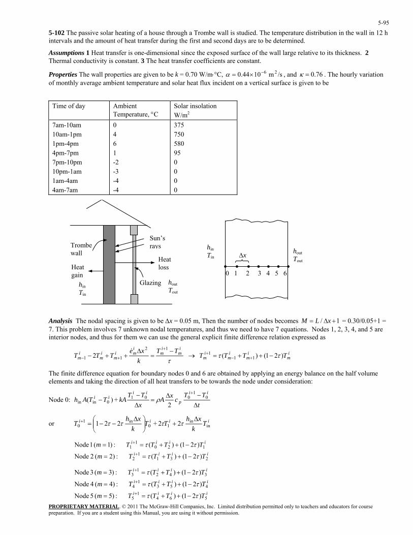
PROPRIETARY MATERIAL. © 2011 The McGraw-Hill Companies, Inc. Limited distribution permitted only to teachers and educators for course preparation. If you are a student using this Manual, you are using it without permission.
5-95
ons 1 Heat transfer is one-dimensional since the exposed surface of the wall large relative to its thickness. 2
⋅°C, , and
5-102 The passive solar heating of a house through a Trombe wall is studied. The temperature distribution in the wall in 12 h intervals and the amount of heat transfer during the first and second days are to be determined.
AssumptiThermal conductivity is constant. 3 The heat transfer coefficients are constant.
/sm 1044.0 26−×=α 76.0=κProperties The wall properties are given to be k = 0.70 W/m . The hourly variation ux incident on a vertical surface is given to be of monthly average ambient temperature and solar heat fl
Time of day Ambient Temperature, °C
Solar insolation W/m2
7am-10am 10am-1pm
4am-7am
0 4 6
-4
375 750
0
1pm-4pm 4pm-7pm 7pm-10pm 10pm-1am 1am-4am
1 -2 -3 -4
580 95 0 0 0
Analysis The nodal spacing is given to be ∆x = 0.05 m, Then the number of nodes becomes = 0.30/0.05+1 = blem involves 7 unknown nodal temperatures, and thus we need to have 7 equations. Nodes 1, 2, 3, 4, and 5 are des, and t us for them we can use the general explicit finite difference relation expressed as
Trombe ∆x
• • • • • • • 0 1 2 3 4 5 6
hinTin
houtTout
wall
Glazing
Sun’s rays
Heat loss Heat
in
gahoutTout
hinTin
1/ +∆= xLM7. This prointerior no h
τ
im
im
imi
mi
mi
mTT
kxe
TTT i −
=∆
++−+
+−
12
11 2&
→ mi
mi
mi
m TTTT )21()( 111 ττ −++= +−+
e difference equation for boundary nodes 0 and 6 are obtained by applying an energy balance on the half volume elements a de under consideration:
Node 0:
The finitnd taking the direction of all heat transfers to be towards the no
tTT
cxAxTT
kATTAhii
p
iiii
∆−∆
=∆−
−+
01
0010inin 2
+)( ρ
or iiii Tk
xhTT
kxh
T inin
10in1
0 22+221∆
+⎟⎟⎠
⎞⎜⎜⎝
⎛ ∆−−=+ ττττ
iiii
iiii
TTTTm
TTTTm
2311
2
1201
1
)21()( :)2( 2 Node
)21()( :)1( 1 Node
ττ
ττ
−++==
−++==+
+
iiii
iiii
iiii
TTTTm
TTTTm
TTTTm
5641
5
4531
4
3421
3
)21()( :)5( 5 Node
)21()( :)4( 4 Node
)21()( :)3( 3 Node
ττ
ττ
ττ
−++==
−++==
−++==
+
+
+

PROPRIETARY MATERIAL. © 2011 The McGraw-Hill Companies, Inc. Limited distribution permitted only to teachers and educators for course preparation. If you are a student using this Manual, you are using it without permission.
5-96
Node 6 t
TTcxA
xTT
kAqATTAhii
p
iiiii
∆−∆
=∆−
+−+
61
665solar6outout 2
+)( ρκ &
or k
xqT
kxh
TTk
xhT
iiiii ∆∆
+⎟⎟⎞
⎜⎜⎛ ∆
−−=+ou
out56
out16 22+221
&κττττ +
⎠⎝solar
t 2τ
where
L = 0.30 m, k = 0.70 W/m.°C, /sm 1044.0 T26−×=α , out and solarq& are as given in the table,
=κ 0.76 , hout = 3.4 W/m2.°C, Tin = 20°C, hin = 9.1 W/m2.°C, and ∆x = 0.05 m.
Next we need to determine the upper limit of the time step ∆t from the stability criteria since we are using the explicit method. This requires the identification of the smallest primary coefficient in the system. We know that the boundary nodes
cient in this case is the coefficient of in the formulation of node 0 since hin >
are more restrictive than the interior nodes, and thus we examine the formulations of the boundary nodes 0 and 6 only. The smallest and thus the most restrictive primary coeffi iT0
hout, and thus
kxh
kxh ∆
−−<∆
−− outin 221221 ττττ
Therefore, the stability criteria for this problem can be expressed as
)/1(2
)/1(2
1 0221in
2
in
in
kxhxt
kxhkxh
∆+∆
≤∆→∆+
≤→≥∆
−−α
τττ
since . Substituting the given quantities, the maximum allowable the time step becomes 2/ xt ∆∆=ατ
s 1722C)] W/m.70.0/(m) 05.0)(C. W/m1.9(1/s)[m 1044.0(2
)m 05.0(226
2=
°°+×≤∆
−t
Therefore, any time step less than 1722 s can be used to solve this problem. For convenience, let us choose the time step to be ∆t = 900 s = 15 min. Then the mesh Fourier number becomes
1584.0)m 05.0(
s) /s)(900m 1044.0(2
26
2=
×=
∆
∆=
−
xtατ
Initially (at 7 am or t = 0), the temperature of the wall is said to vary linearly between 20°C at node 0 and 0°C at node 6. Noting that there are 6 nodal spacing of equal length, the temperature change between two neighboring nodes is (20 - 0)°C/6 = 3.33°C. Therefore, the initial nodal temperatures are
Substituting the given and calculated quantities, the nodal temperatures after 6, 12, 18, 24, 30, 36, 42, and 48 h are calculated and presented in the following table and chart.
C0 C,33.3 C,66.6 C,10 C,33.13 C,66.16 C,20 06
05
04
03
02
01
00 °=°=°=°=°=°=°= TTTTTTT
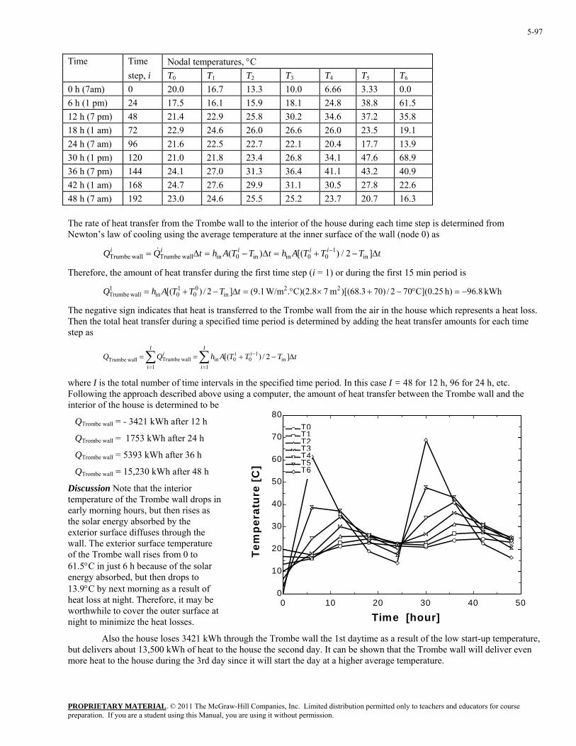
PROPRIETARY MATERIAL. © 2011 The McGraw-Hill Companies, Inc. Limited distribution permitted only to teachers and educators for course preparation. If you are a student using this Manual, you are using it without permission.
5-97
Time Time Nodal temperatures, °C step, i T0 T1 T2 T3 T4 T5 T6
0 h (7am) 0 20.0 16.7 13.3 10.0 6.66 3.33 0.0 6 h (1 pm) 24 17.5 16.1 15.9 18.1 24.8 38.8 61.5 12 h (7 pm) 48 21.4 22.9 25.8 30.2 34.6 37.2 35.8 18 h (1 am) 72 22.9 24.6 26.0 26.6 26.0 23.5 19.1 24 h (7 am) 96 21.6 22.5 22.7 22.1 20.4 17.7 13.9 30 h (1 pm) 120 21.0 21.8 23.4 26.8 34.1 47.6 68.9 36 h (7 pm) 144 24.1 27.0 31.3 36.4 41.1 43.2 40.9 42 h (1 am) 168 24.7 27.6 29.9 31.1 30.5 27.8 22.6 48 h (7 am) 192 23.0 24.6 25.5 25.2 23.7 20.7 16.3
t transfeThe rate of heaewton’s law o
r from the Trombe wall to the interior of the house during each time step is determined from f cooling using the average temperature at the inner surface of the wall (node 0) as
iiii ∆−+=∆−=∆= − ]2/)[()( in1
00inin0in wallTrumbe wallbe&
ount of heat transfer during the first time step (i = 1) or during the first 15 min period is 22
in0 −=°−+×°=∆− tT
loss. e
=
∆ii
t11
]
ified time period. In this case I = 48 for 12 h, 96 for 24 h, etc. wing the approach described above using a computer, the amount of heat transfer between the Trombe wall and the
kWh after 12 h
r
eat loss at night. Therefore, it may be worthwhile to cover the outer surface at night to minimize the heat losses.
Also the house loses 3421 kWh through the Trombe wall the 1st daytime as a result of the low start-up temperature, but delivers about 13,500 kWh of heat to the house the second day. It can be shown that the Trombe wall will deliver even more heat to the house during the 3rd day since it will start the day at a higher average temperature.
N
Qium tTTTAhtTTAhtQTr
Therefore, the am
[( 010in
1 wallTrumbe += TTAhQ kWh 8.96h) 25.0](C702/)703.68)[(m 7C)(2.8. W/m1.9(]2/)
The negative sign indicates that heat is transferred to the Trombe wall from the air in the house which represents a heateach timThen the total heat transfer during a specified time period is determined by adding the heat transfer amounts for
step as
∑∑ − −+== iii TTTAhQQ in1
00in wallTrumbe wallTrumbe 2/)[(II
=
where I is the total number of time intervals in the specFollointerior of the house is determined to be
QTrombe wall = - 3421
0 10 20 30 40 50
80
QTrombe wall = 1753 kWh after 24 h
QTrombe wall = 5393 kWh after 36 h
QTrombe wall = 15,230 kWh after 48 h
Discussion Note that the interiotemperature of the Trombe wall drops in early morning hours, but then rises as the solar energy absorbed by the exterior surface diffuses through the wall. The exterior surface temperature of the Trombe wall rises from 0 to 61.5°C in just 6 h because of the solar energy absorbed, but then drops to 13.9°C by next morning as a result of h
0
10
20
30
40
50
60
70
Time [hour]
e
T0T0T1T1T2T2T3T3T4T4T5T5T6T6]
[CTe
mpe
ratu
r
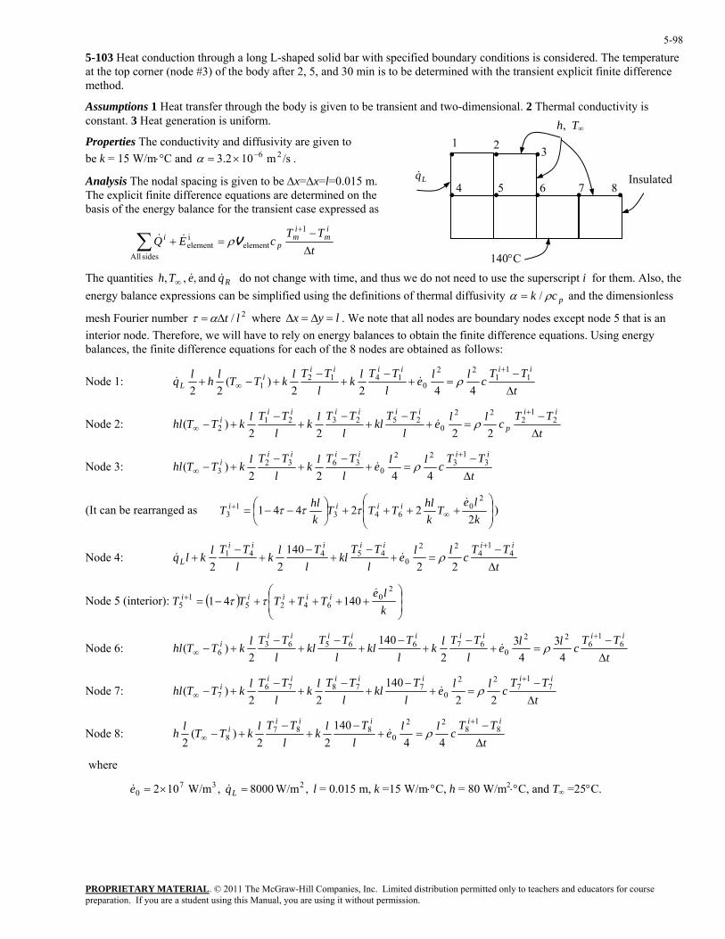
PROPRIETARY MATERIAL. © 2011 The McGraw-Hill Companies, Inc. Limited distribution permitted only to teachers and educators for course preparation. If you are a student using this Manual, you are using it without permission.
5-98
-103 Heat conduction through a long L-shaped solid bar with specified boundary conditions is considered. The temperature at t cor node f the b after and 3 to be determ with t ansient explicit finite difference me .
Assumptions tra rou bod en trans tw nsi Thermal conductivity is constant. 3 H era nif
Properties Th duct d d ty a n tobe 5 W/ d 1× .
An is The nodal spacing is given to be ∆x 0.0Th icit f ffe ua e d ed bas the e ala the nt c res
5he top thod
ner ( #3) o ody 2, 5, 0 min is ined he tr
1 Heateat gen
nsfer thtion is u
gh the orm.
y is giv to be ient and o-dime onal. 2
e con ivity an iffusivi re give k = 1 m⋅°C an /sm 0 26−2.3=α
alys =∆x=l= 15 m. e expl inite di rence eq tions ar etermin on the is of nergy b nce for transie ase exp sed as
tT i
m−+1TcE
im
p∑ elementiele
si All
Vρ&
Th itie &, , do not change with tim hus not us pe t i for them. Also, the ene lan ss be ied the ons ma ivit d the dimensionless
me rier r τ x
Qi&∆
=+ mentdes
e quant s Th , Rq& and
• • •
14
32
6 7 8 • • • •
, T∞
0°C
1
4 5 •
h
InsulatedLq&
e∞ e, and t we do need to e the su rscriprgy ba ce expre ions can simplif using definiti of ther l diffus y kα = pcρ an/
2/ l lt∆=α where sh Fou numbe y =∆=∆ . e th de un des pt node 5 that is an inte de ore ll h ely rgy es n th di eq s. Using energy balances, the finite difference equations for e the s ar ed ws
Node 1:
We not at all no s are bo dary no excerior no . Theref , we wi ave to r on ene balanc to obtai e finite fference uation
ach of 8 node e obtain as follo :
t∆T ii −+
11T
lTll
=−
+−∞1
2
422
ode 2:
c4
ρ l 2li1 e+ 0&
Tl i4k
2lTT ii − 12kT +1 )Th+ (
2lqL&
i
tTT
cllel
TTkl
lTTlk
lTTlkTThl
ii
pNiiii
i
∆−
=+−
+−
+−
+−∞2
12
2
0252321
2 2222)( ρ&
Node 3:
ii +2
tTT
cllel
TTlkl
TTlkTThliiiiii
i
∆−
=+−
+−
+−+
∞3
13
22
03632
3 4422)( ρ&
⎟⎟⎠
⎞⎜⎜⎝
⎛++++⎟
⎠⎞
⎜⎝⎛ −−= ∞
+
kle
TkhlTTT
khlT iiii
222441
20
6431
3&
τττ ) (It can be rearranged as
tTT
cllel
TTkl
lTlk
lTTlklq
iiiiiii
L ∆−
=+−
+−
+−
++
41
422
045441
22140
22ρ&& Node 4:
Node 5 (interior): ( ) ⎟⎟⎠
⎞⎜⎜⎝
⎛+++++−=+
kle
TTTTT iiiii2
06425
15 14041
&ττ
tTT
cllel
TTlkl
Tkl
lTT
kll
TTlkTThliiiiiiiii
i
∆−
=+−
+−
+−
+−
+−+
∞6
16
22
06766563
6 43
43
2140
2)( ρ& Node 6:
tTT
cllel
Tkl
lTTlk
lTTlkTThl
iiiiiiii
∆−
=+−
+−
+−
+−+
∞7
17
22
077876
7 22140
22)( ρ& Node 7:
tTT
cllel
Tlkl
TTlkTTlhiiiii
i
∆−
=+−
+−
+−+
∞8
18
22
0887
8 44140
22)(
2ρ& Node 8:
where
l = 0.015 m, k =15 W/m⋅°C, h = 80 W/m2⋅°C, and T∞ =25°C. , W/m8000 , W/m102 2370 =×= Lqe &&
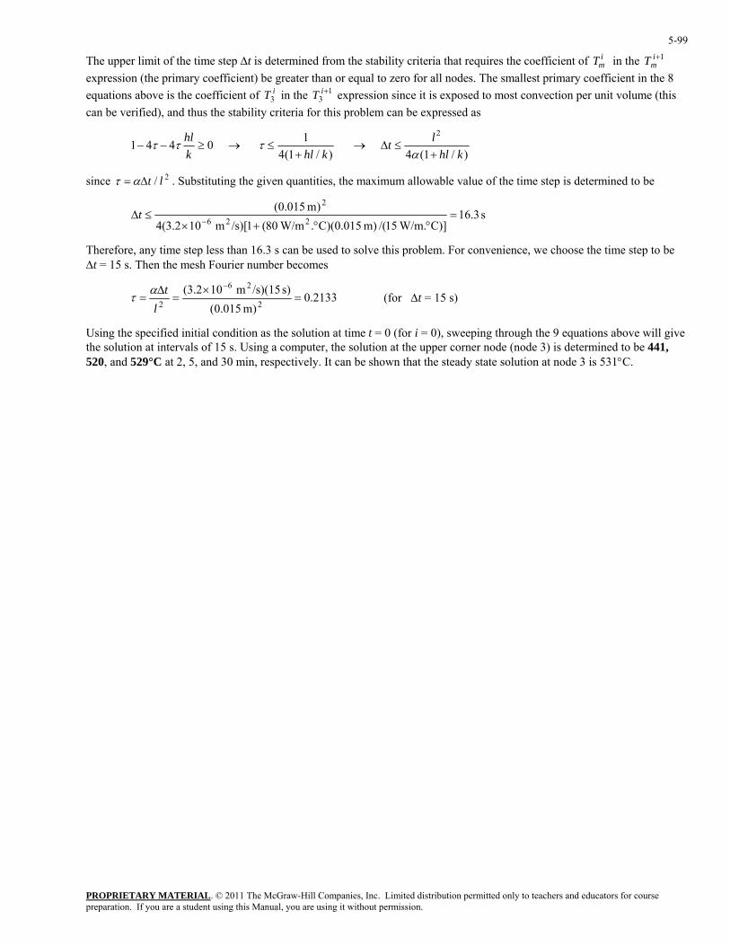
PROPRIETARY MATERIAL. © 2011 The McGraw-Hill Companies, Inc. Limited distribution permitted only to teachers and educators for course preparation. If you are a student using this Manual, you are using it without permission.
5-99
The upper limit of the time step ∆t is determined from the stability criteria that requires the coefficient of imT in the 1+i
mT expression (the primary coefficient) be greater than or equal to zero for all nodes. The smallest primary coefficient in the 8 equations above is the coefficient of iT3 in the 1
3+iT expression since it is exposed to most convection per unit volume (this
can be verified), and thus the stability criteria for this problem can be expressed as
1 4 4 0 14 1 4 1
2− − ≥ → ≤
+→ ≤
+τ τ τ
αhlk hl k
t lhl k
( / ) ( /
∆
2
)
since =τ . Substituting the given quantities, the maximum allowable value of the time step is determined to be / lt∆α
s 3.16C)] W/m.15/(m) 015.0)(C. W/m80(1/s)[m 102.3(4
)m 015.0(226
2=
°°+×≤∆
−t
Therefore, any time step less than 16.3 s can be used to solve this problem. For convenience, we choose the time step to be ∆t = 15 s. Then the mesh Fourier number becomes
2133.0)m 015.0(
10.3(2
6
2=
×==
−
lτ (for ∆t = 15 s)
Using the specified initial condition as the solution at time t = 0 (for i = 0), sweeping through the 9 equations above will givthe solution at intervals of 15 s
s) /s)(15m 2 2∆tα
e . Using a computer, the solution at the upper corner node (node 3) is determined to be 441,
9°C at 2, 5, and 30 min, respectively. It can be shown that the steady state solution at node 3 is 531°C. 520, and 52
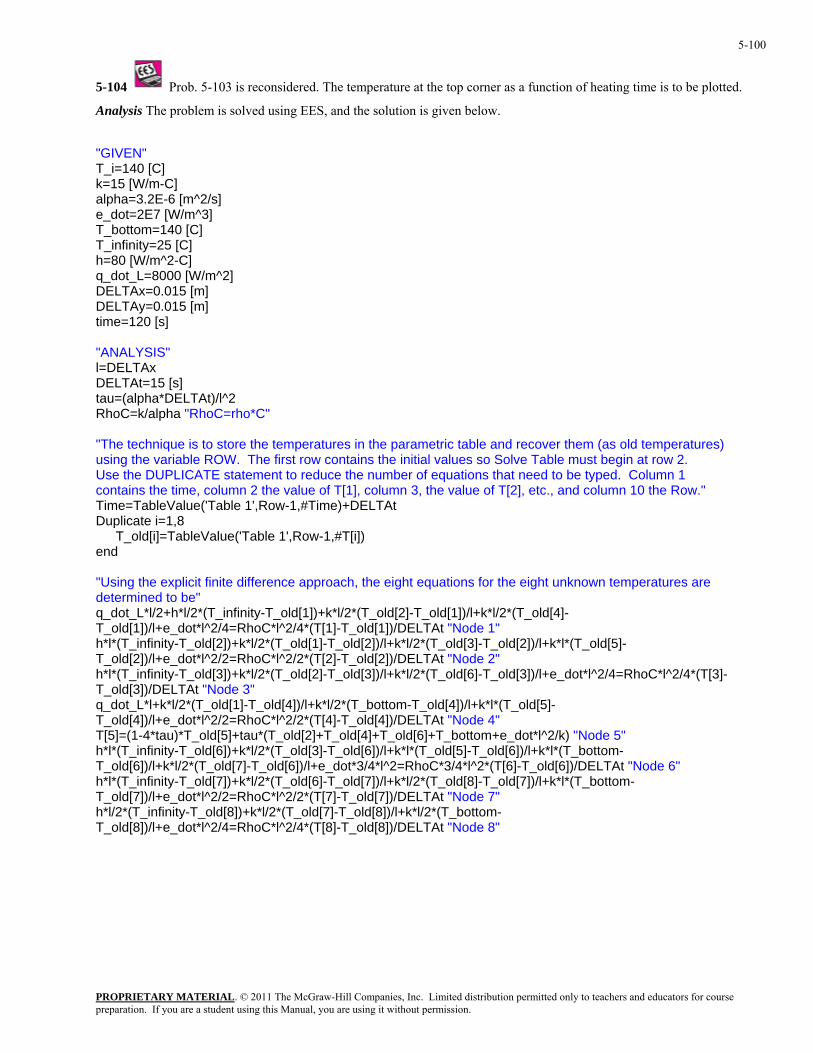
PROPRIETARY MATERIAL. © 2011 The McGraw-Hill Companies, Inc. Limited distribution permitted only to teachers and educators for course preparation. If you are a student using this Manual, you are using it without permission.
5-100
5-104 Prob. 5-103 is reconsidered. The temperature at the top corner as a function of heating time is to be plotted.
T_i=140 [C] k=
T_infinity=25 [C] h=80 [W/m^2-C] q_dot_L=8000 [W/m^2] DELTAx=0.015 [m] DELTAy=0.015 [m] time=120 [s] "ANALYSIS" l=DELTAx DELTAt=15 [s] tau=(alpha*DELTAt)/l^2 RhoC=k/alpha "RhoC=rho*C" "The technique is to store the temperatures in the parametric table and recover them (as old temperatures) using the variable ROW. The first row contains the initial values so Solve Table must begin at row 2. Use the DUPLICATE statement to reduce the number of equations that need to be typed. Column 1 contains the time, column 2 the value of T[1], column 3, the value of T[2], etc., and column 10 the Row." Time=TableValue('Table 1',Row-1,#Time)+DELTAt Duplicate i=1,8 T_old[i]=TableValue('Table 1',Row-1,#T[i]) end "Using the explicit finite difference approach, the eight equations for the eight unknown temperatures are determined to be" q_dot_L*l/2+h*l/2*(T_infinity-T_old[1])+k*l/2*(T_old[2]-T_old[1])/l+k*l/2*(T_old[4]-T_old[1])/l+e_dot*l^2/4=RhoC*l^2/4*(T[1]-T_old[1])/DELTAt "Node 1" h*l*(T_infinity-T_old[2])+k*l/2*(T_old[1]-T_old[2])/l+k*l/2*(T_old[3]-T_old[2])/l+k*l*(T_old[5]-T_old[2])/l+e_dot*l^2/2=RhoC*l^2/2*(T[2]-T_old[2])/DELTAt "Node 2" h*l*(T_infinity-T_old[3])+k*l/2*(T_old[2]-T_old[3])/l+k*l/2*(T_old[6]-T_old[3])/l+e_dot*l^2/4=RhoC*l^2/4*(T[3]-T_old[3])/DELTAt "Node 3" q_dot_L*l+k*l/2*(T_old[1]-T_old[4])/l+k*l/2*(T_bottom-T_old[4])/l+k*l*(T_old[5]-T_old[4])/l+e_dot*l^2/2=RhoC*l^2/2*(T[4]-T_old[4])/DELTAt "Node 4" T[5]=(1-4*tau)*T_old[5]+tau*(T_old[2]+T_old[4]+T_old[6]+T_bottom+e_dot*l^2/k) "Node 5" h*l*(T_infinity-T_old[6])+k*l/2*(T_old[3]-T_old[6])/l+k*l*(T_old[5]-T_old[6])/l+k*l*(T_bottom-T_old[6])/l+k*l/2*(T_old[7]-T_old[6])/l+e_dot*3/4*l^2=RhoC*3/4*l^2*(T[6]-T_old[6])/DELTAt "Node 6" h*l*(T_infinity-T_old[7])+k*l/2*(T_old[6]-T_old[7])/l+k*l/2*(T_old[8]-T_old[7])/l+k*l*(T_bottom-T_old[7])/l+e_dot*l^2/2=RhoC*l^2/2*(T[7]-T_old[7])/DELTAt "Node 7" h*l/2*(T_infinity-T_old[8])+k*l/2*(T_old[7]-T_old[8])/l+k*l/2*(T_bottom-T_old[8])/l+e_dot*l^2/4=RhoC*l^2/4*(T[8]-T_old[8])/DELTAt "Node 8"
Analysis The problem is solved using EES, and the solution is given below.
"GIVEN"
15 [W/m-C] alpha=3.2E-6 [m^2/s] e_dot=2E7 [W/m^3] T_bottom=140 [C]
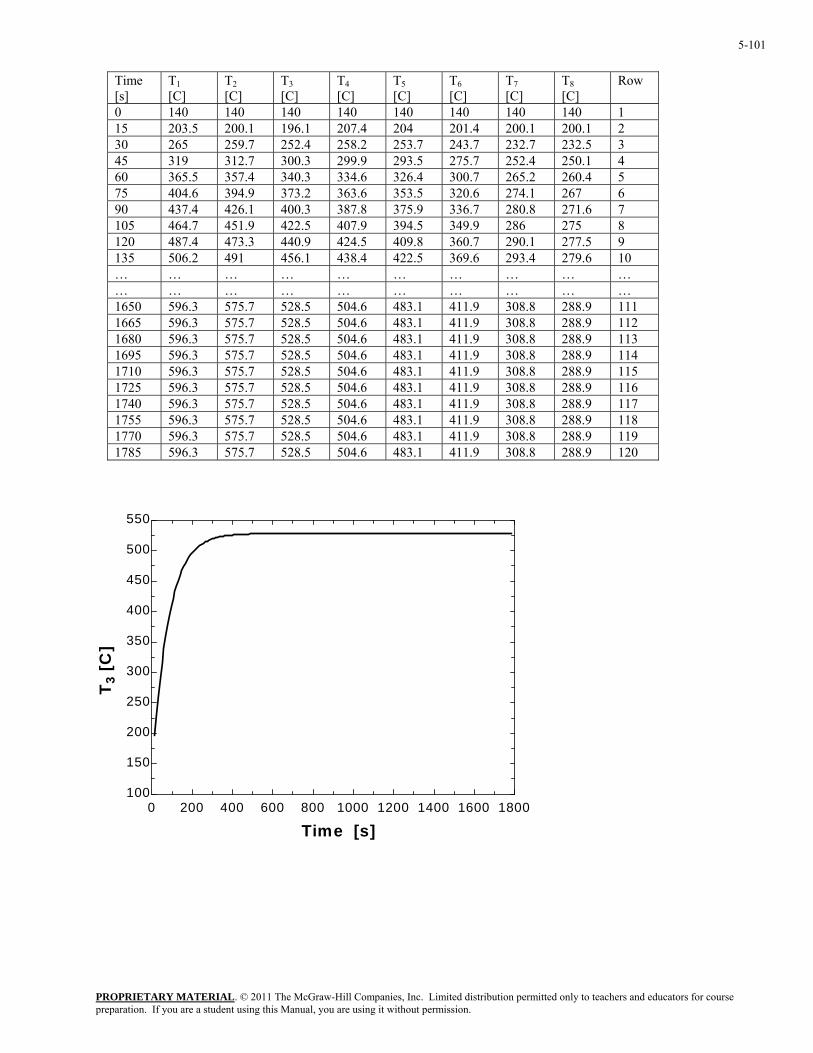
PROPRIETARY MATERIAL. © 2011 The McGraw-Hill Companies, Inc. Limited distribution permitted only to teachers and educators for course preparation. If you are a student using this Manual, you are using it without permission.
5-101
Time [s]
T1 [C]
T2 [C]
T3 [C]
T4 [C]
T5 [C]
T6 [C]
T7 [C]
T8 [C]
Row
0 140 140 140 140 140 140 140 140 1 15 203.5 200.1 196.1 207.4 204 201.4 200.1 200.1 2 30 265 259.7 252.4 258.2 253.7 243.7 232.7 232.5 3 45 319 312.7 300.3 299.9 293.5 275.7 252.4 250.1 4 60 365.5 357.4 340.3 334.6 326.4 300.7 265.2 260.4 5 75 404.6 394.9 373.2 363.6 353.5 320.6 274.1 267 6 90 437.4 426.1 400.3 387.8 375.9 336.7 280.8 271.6 7 105 464.7 451.9 422.5 407.9 394.5 349.9 286 275 8 120 487.4 473.3 440.9 424.5 409.8 360.7 290.1 277.5 9 135 506.2 491 456.1 438.4 422.5 369.6 293.4 279.6 10 … … … … … … … … … … … … … … … … … … … … 1650 596.3 575.7 528.5 504.6 483.1 411.9 308.8 288.9 111 1665 596.3 575.7 528.5 504.6 483.1 411.9 308.8 288.9 112 1680 596.3 575.7 528.5 504.6 483.1 411.9 308.8 288.9 113 1695 596.3 575.7 528.5 504.6 483.1 411.9 308.8 288.9 114 1710 596.3 575.7 528.5 504.6 483.1 411.9 308.8 288.9 115 1725 596.3 575.7 528.5 504.6 483.1 411.9 308.8 288.9 116 1740 596.3 575.7 528.5 504.6 483.1 411.9 308.8 288.9 117 1755 596.3 575.7 528.5 504.6 483.1 411.9 308.8 288.9 118 1770 596.3 575.7 528.5 504.6 483.1 411.9 308.8 288.9 119 1785 596.3 575.7 528.5 504.6 483.1 411.9 308.8 288.9 120
0 200 400 600 800 1000 1200 1400 1600 1800100
150
200
250
300
350
400
450
500
550
Time [s]
T 3 [C
]
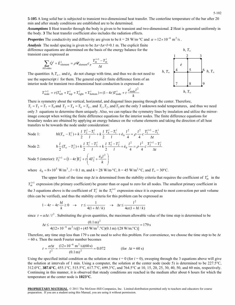
PROPRIETARY MATERIAL. © 2011 The McGraw-Hill Companies, Inc. Limited distribution permitted only to teachers and educators for course preparation. If you are a student using this Manual, you are using it without permission.
5-102
0
dimensional. 2 Heat is generated uniformly in
. explicit finite
5-105 A long solid bar is subjected to transient two-dimensional heat transfer. The centerline temperature of the bar after 2min and after steady conditions are established are to be determined. Assumptions 1 Heat transfer through the body is given to be transient and two-the body. 3 The heat transfer coefficient also includes the radiation effects. Properties The conductivity and diffusivity are given to be k = 28 W/m⋅°C and =αAnalysis The nodal spacing is given to be ∆x=∆x=l=0.1 m. The
/sm 1012 26−×
difference equations are determined on the basis of the energy balance for thetransient case expressed as
• • •
4 5 6
• • •
• • •h, T∞
1 2 3
7 8 9
h, T∞
h, T∞
e& tTT
cEQ mmp
i
∆−
=+∑ elementielement
sides All
Vρ&&
The quantities 0 and , , eTh &∞
ii+1
do not change with time, and thus we do not need to use the superscript i for them. The general explicit finite difference form of an
h, T∞
interior node for transient two-dimensional heat conduction is expressed as
kle
TTTTTT i2i
nodeinode
ibottom
iright
itop
ileft
1node )41()(
&τττ +−++++=+
There is symmetry about the vertical, horizontal, and diagonal lines passing through the center. Therefore, and , and are the only 3 unknown noda tures, and thus we need
ations to determine them uniquely. Also, we can replace the symmetry lines by insulation and utilize the mirror-image concept when writing the finite difference equations for the interior nodes. The finite difference equations for
applying an energy balance on the volume elements and taking the direction of all heat be towa s the node under consideration:
9731 TTTT === 8642 TTTT === 521 and ,, TTT l temperaonly 3 equ
boundary nodes are obtained bytransfers to rd
tTT
cllel
TTlkl
TTlkTThliiiiii
i
∆−
=+−
+−
+−+
∞1
11
22
01412
1 4422)( ρ& Node 1:
tTT
cllel
TTlkl
TTlkTTlhiiiiii
i
∆−
=+−
+−
+−+
∞2
12
22
02521
2 4422)(
2ρ& Node 2:
Node 5 (interior): ( ) ⎟⎟⎠
⎞⎜⎜⎝
⎛++−=+
kle
TTT iii2
025
15 441
&ττ
350 W/m108×=where e& , l = 0.1 m, and k = 28 W/m⋅°C, h = 45 W/m2⋅°C, and T∞ = 30°C.
he upper limit of the time step ∆t is determined from the stability criteria that requires the coefficient of in the
expression (the primary coefficient) be greater than or equal to zero for all nodes. The smallest primary coefficient in
tions abov is the coefficient of in the expression since it is exposed to most convection per unit volume (this can be verified), and thus the stability criteria for this problem can be expressed as
T imT
1+imT
iT11
1+iTthe 3 equa e
)/1(4
)/1(4
1 04412
khllt
khlkhl
+≤∆→
+≤→≥−−
ατττ
since ∆=ατ um allowable value of the time step is determined to be 2/ lt . Substituting the given quantities, the maxim
s 179C)] W/m.28/(m) 1.0)(C. W/m45(1/s)[m 1012(4 226 °+×
≤∆−
t)m 1.0( 2
=°
Therefore, any time step less than 179 s can be used to solve this problem. For convenience, we choose the time step to be ∆t = 60 s. Then the mesh Fourier number becomes
072.0)m 1.0(
s) /s)(60m 1012(2
26
2=
×=
∆=
−
ltατ (for ∆t = 60 s)
Using the specified initial condition as the solution at time t = 0 (for i = 0), sweeping through the 3 equations above will give the solution at intervals of 1 min. Using a computer, the solution at the center node (node 5) is determined to be 227.5°C, 312.0°C, 387.6°C, 455.1°C, 515.5°C, 617.7°C, 699.3°C, and 764.5°C at 10, 15, 20, 25, 30, 40, 50, and 60 min, respectively. Continuing in this manner, it is observed that steady conditions are reached in the medium after about 6 hours for which the temperature at the center node is 1023°C.
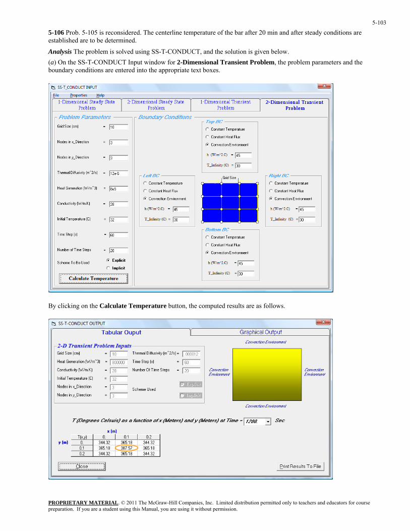
PROPRIETARY MATERIAL. © 2011 The McGraw-Hill Companies, Inc. Limited distribution permitted only to teachers and educators for course preparation. If you are a student using this Manual, you are using it without permission.
5-103
di
Transient Problem, the problem parameters and the boundary conditions are entered into the appropriate text boxes.
5-106 Prob. 5-105 is reconsidered. The centerline temperature of the bar after 20 min and after steady con tions areestablished are to be determined.
Analysis The problem is solved using SS-T-CONDUCT, and the solution is given below. (a) On the SS-T-CONDUCT Input window for 2-Dimensional
By clicking on the Calculate Temperature button, the computed results are as follows.
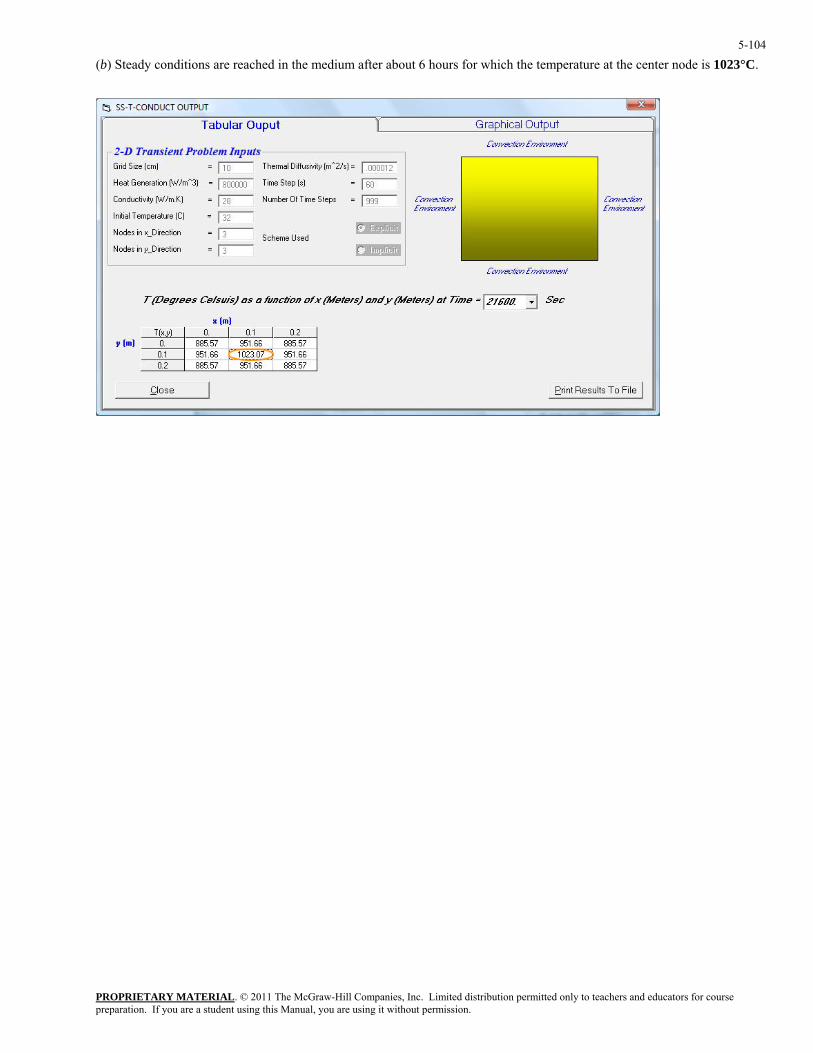
PROPRIETARY MATERIAL. © 2011 The McGraw-Hill Companies, Inc. Limited distribution permitted only to teachers and educators for course preparation. If you are a student using this Manual, you are using it without permission.
5-104
(b) Steady conditions are reached in the medium after about 6 hours for which the temperature at the center node is 1023°C.
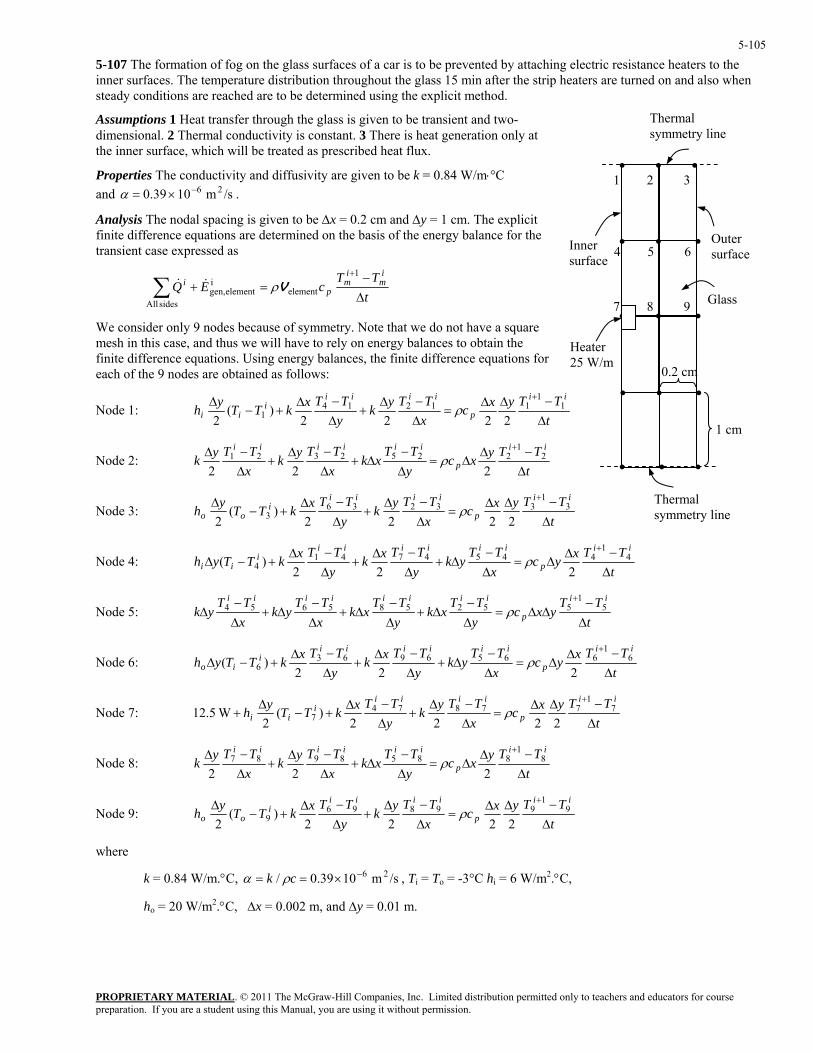
PROPRIETARY MATERIAL. © 2011 The McGraw-Hill Companies, Inc. Limited distribution permitted only to teachers and educators for course preparation. If you are a student using this Manual, you are using it without permission.
5-105
the explicit method.
neration only at
ty are given to be k = 0.84 W/m⋅°C
1 cm. The exnergy balance f
5-107 The formation of fog on the glass surfaces of a car is to be prevented by attaching electric resistance heaters to theinner surfaces. The temperature distribution throughout the glass 15 min after the strip heaters are turned on and also whensteady conditions are reached are to be determined using
Assumptions 1 Heat transfer through the glass is given to be transient and two-dimensional. 2 Thermal conductivity is constant. 3 There is heat gethe inner surface, which will be treated as prescribed heat flux.
Properties The conductivity and diffusivi26−
• • •
and /sm 1039.0 ×=α .
Analysis The nodal spacing is given to be ∆x = 0.2 cm and ∆y =finite difference equations are determined on the basis of the etransient case expressed as
plicit or the
tTT
EQii
i −+
+
∑1
igen,&& c mm
p ∆= elementelement
sides All
Vρ
metry. Note that we do not have a square mesh in this case, and thus we will have to rely on energy balances to obtain the
e nce equations. Using energy balances, the finite difference equations for
We consider only 9 nodes because of sym
finite diff reeach of the 9 nodes are obtained as follows:
Node 1: t
TTyxxTTyk
yTTxkTTyh
iiiii
ii∆
=∆−∆
+∆−∆
+−∆ 1214
1 22)(
2ρc p ∆
−∆ 11
22
Node 2:
ii+1
tTTyxc
yTT
xkxTTyk
xTTyk
ii
p
iiiiii
∆−∆
∆=∆−
∆+∆−∆
+∆−∆ +
21
2252321
222ρ
Node 3: t
TTyxcxTTyk
yTTxkTTyh
ii
p
iiiii
oo ∆−∆∆
=∆−∆
+∆−∆
+−∆ +
31
332363 2222
)(2
ρ
Heater 25 W/m
Thermal symmetry line
0.2 cm
1 cm
Outer surface
1 2 3
Glass
Inner surface
• • •
• • •
• • •
• • •
4 5 6
7 8 9
Thermal symmetry line
tTTxyc
xTT
ykyTTxk
yTTxkTTyh
ii
p
iiiiiii
ii ∆−∆
∆=∆−
∆+∆−∆
+∆−∆
+−∆+
41
44547414 222
)( ρ Node 4:
Node 5: t
yxcy
xky
xkx
ykx
yk p ∆∆∆=
∆∆+
∆∆+
∆∆+
∆∆ 55258565 ρ
TTTTTTTTTT iiiiiiiiii −−−−− +5
14
Node 6: t
TTxycxTT
ykyTTxk
yTTxkTTyh
ii
p
iiiiiii
io ∆−∆
∆=∆−
∆+∆−∆
+∆−∆
+−∆+
61
66569636 222
)( ρ
Node 7: t
TTyxcxTTyk
yTTxkTTyh p
iii ∆
−∆∆=
∆−∆
+∆−∆
+−∆
+ 7778747 2222
)(2
W5.12 ρ iiiiii +1
tTTyxc
TTxk
TTykTTyk
iiiiiii ∆∆=
−∆+
−∆+
−∆ +18858987 ρ
yxx
i
p ∆−
∆∆∆8
222 Node 8:
tTTyxc
xk
ykTTh poo =
∆+
∆+− 9 22
)(2
ρNode 9: TTyTTxy iiiii
i
∆−∆∆−∆−∆∆ +
91
99896
22
where
k = 0.84 W/m.°C, Ti = To = -3°C hi = 6 W/m2.°C,
ho = 20 W/m2.°C, ∆x = 0.002 m, and ∆y = 0.01 m.
i
/sm 1039.0/ 26−×== ck ρα ,
PROPRIETARY MATERIAL. © 2011 The McGraw-Hill Companies, Inc. Limited distribution permitted only to teachers and educators for course preparation. If you are a student using this Manual, you are using it without permission.
5-106
e stability criteria that requires the coefficient of in the xpression (the primary coefficient) be greater than or equal to zero for all nodes. The smallest primary coefficient in the 9
imT 1+i
mT The upper limit of the time step ∆t is determined from theequations above is the coefficient of iT6 in the 1
6+iT expression since it is exposed to most convection per unit volume (this
can be verified). The equation for node 6 can be rearranged as
⎟⎟⎠
⎞⎜⎜⎝
⎛
∆+
∆
++
∆∆+
⎥⎥⎦
⎤
⎢⎢⎣
⎡⎟⎟⎠
⎞⎜⎜⎝
⎛
∆+
∆+
∆∆−=+
25
293
06221
6 21121x
Ty
TTT
xkh
tTxyxk
htT
iiioioi αα
Therefore, the stability criteria for this problem can be expressed as
⎟⎟⎠
⎞⎜⎜⎝
⎛
∆+
∆+
∆
⎟⎠
⎜⎝ ∆∆∆
22
22 112xyxk
hxyxk oα
Substituting the given quantities, the maximum allowable value of the time step is determined to be
or,
≤∆→≥⎟⎞
⎜⎛
++∆−1t 01121
ht oα
s 7.4
m) 01.0()m 002.0(m) 002.0)(C W/m84.0()/m 1039.0(2
2226
⎟⎟⎠
⎜⎜⎝
++°⋅
×× s
Therefore, any time step less than 4.8 s can be used to solve this problem. For convenience, we choose the time
11C W/m20
1t2
=⎞⎛ °⋅
≤∆
step to be ∆t 4 s. Then the temperature distribution throughout the glass 15 min after the strip heaters are turned on and when steady
ined to be (from the EES solutions in CD)
T = -0.73°C, T = -0.84°C, T = -0.98°C, T = 0.68°C, T = -0.03°C,
T6 = -2.0 C, T7 = 36.0 C, T8 = 32.0 C, T9 = 29.2 C
Steady-state: T1 = -0.69°C, T2 = -0.79°C, T3 = -0.93°C, T4 = 0.71°C, T5 °C,
T = -2.0°C, T = 36.1°C, T = 32.0°C, T = 29.2°C
=conditions are reached are determ
15 min: 1 2 3 4 5
° ° ° °
= -0.005
6 7 8 9
Discussion Steady operating conditions are reached in about 10 min.
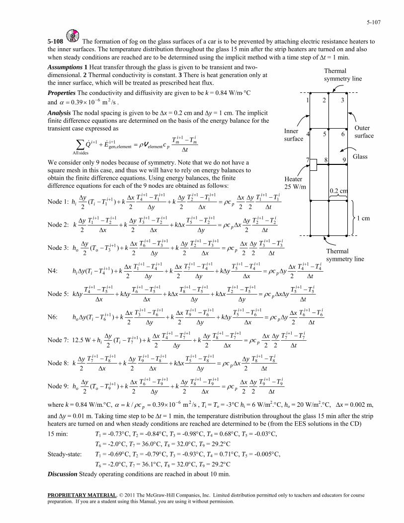
PROPRIETARY MATERIAL. © 2011 The McGraw-Hill Companies, Inc. Limited distribution permitted only to teachers and educators for course preparation. If you are a student using this Manual, you are using it without permission.
5-107
5-108 The formation of fog on the glass surfaces of a car is to be prevented by attaching electric resistance heaters to the inner surfaces. The temperature distribution throughout the glass 15 min after the strip heaters are turned on and also
step of ∆t = 1 min. Assumptions 1 Heat transfer through the glass is given to be transient and two-
nsional. 2 Thermal conductivity is constant. 3 There is heat generation only at the inner surface, which will be treated as prescribed heat flux.
alanp sed as
when steady conditions are reached are to be determined using the implicit method with a time
dime
Properties The conductivity and diffusivity are given to be k = 0.84 W/m⋅°C and /sm 1039.0 26−×=α . Analysis The nodal spacing is given to be ∆x = 0.2 cm and ∆y = 1 cm. The implicit finite difference equations are determined on the basis of the energy b ce for the transient case ex res
• • • 1 2 3
tTT
cEQi
mi
mp
i
∆−
=++
+∑1
element1+i
elementgen,sides All
1 Vρ&&
We consider only 9 nodes because of symmetry. Note that we do not have a uare mesh in this case, and thus we will have to rely on energy balances to
btain the finite difference equations. Using energy balances, the finite sqodifference equations for each of the 9 nodes are obtained as follows:
Node 1: t
TTyxcxTTyk
yTTxkTTyh
ii
p
iiiii
ii ∆−∆∆
=∆−∆
+∆−∆
+−∆ +++++
+ 11
11
11
21
11
411 2222
)(2
ρ
Node 2: t
TTyxcyTT
xkxTTyk
xTTyk
ii
p
iiiiii
∆−∆
∆=∆−
∆+∆−∆
+∆−∆ +++++++
21
21
21
51
21
31
21
1
222ρ
Node 3: t
TTyxcxTTyk
yTTxkTTyh
iiiiii −−− +++++ 11111
pi
oo ∆∆∆
=∆
∆+
∆∆
+−∆ + 3332361
3 2222)(
2ρ
N4: t
TTxycx
yky
xkyTTxkTTyh p
iii ∆
∆∆=
∆∆+
∆∆
+∆
∆+−∆ + 444547411
4 222)( ρ
TTTT iiiiiiii −−−− +++++++ 1111111
Heater
Thermal symmetry line
1 cm
Outer
Glass
Inner • surfacesurface
25 W/m 0.2 cm
• •
• • •
• • •
• • •
4 5 6
7 8 9
Thermal symmetry line
tTT
yxcyTT
xkyTT
xkxTT
ykxTT
ykii
p
iiiiiiii
∆−
∆∆=∆−
∆+∆−
∆+∆−
∆+∆−
∆+++++++++
51
51
51
21
51
81
51
61
51
4 ρ Node 5:
N6: txyy pio ∆∆∆∆6 222
Node 7:
TTxycTT
ykTTxk
TTxkTTyhiiiiiiii
i −∆∆=
−∆+
−∆+
−∆+−∆
++++++++ 6
16
16
15
16
19
16
131 )( ρ
tTTyxTTyTTxkTTyh
iiiiiii
ii−∆∆−∆−∆
+−∆
++++++
+1111
71
417 )( W5.12 c
xk
y p ∆=
∆+
∆7778
22222ρ
ode 8:N tyxx ∆∆∆∆ 222
Node 9:
TTyxcTT
xkTTyk
TTykii
p
iiiiii −∆∆=
−∆+
−∆+
−∆ +++++++8
18
18
15
18
19
18
17 ρ
tTTyxc
xTTyk
yTTxkTTyh
ii
p
iiiii
oo ∆−∆∆
=∆−∆
+∆−∆
+−∆ +++++
+ 91
91
91
81
91
619 2222
)(2
ρ
26− 2 2where k = 0.84 W/m.°C, ×== pck ρα , Ti = To = -3°C hi = 6 W/m .°C, ho = 20 W/m .°C, ∆x = 0.002 m,
and ∆y = 0.01 m. Taking time step to be ∆t = 1 min, the temperature distribution throughout the glass 15 min after the strip heaters are turned on and when steady conditions are reached are determined to be (from the EES solutions in the CD) 15 min: T1 = -0.73°C, T2 = -0.84°C, T3 = -0.98°C, T4 = 0.68°C, T5 = -0.03°C,
T6 = -2.0°C, T7 = 36.0°C, T8 = 32.0°C, T9 = 29.2°C Steady-state: T1 = -0.69°C, T2 = -0.79°C, T3 = -0.93°C, T4 = 0.71°C, T5 = -0.005°C,
T6 = -2.0°C, T7 = 36.1°C, T8 = 32.0°C, T9 = 29.2°C Discussion Steady operating conditions are reached in about 10 min.
/sm 1039.0/
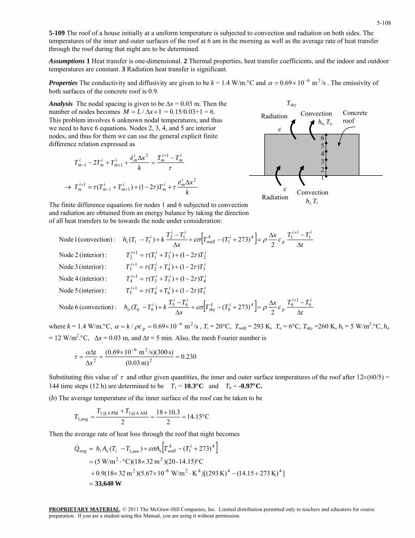
PROPRIETARY MATERIAL. © 2011 The McGraw-Hill Companies, Inc. Limited distribution permitted only to teachers and educators for course preparation. If you are a student using this Manual, you are using it without permission.
5-108
use initially at a uniform temperature is subjected to convection and radiation on both sides. The mperatures of the inner and outer surfaces of the roof at 6 am in the morning as well as the average rate of heat transfer rough the roof during that night are to be determined.
roperties, heat transfer coefficients, and the indoor and outdoor ant.
.4 W/m.° . The emissivity of roof is 0.9.
0.03 m. Then the
eior
5-109 The roof of a hoteth
Assumptions 1 Heat transfer is one-dimensional. 2 Thermal ptemperatures are constant. 3 Radiation heat transfer is signific
Properties The conductivity and diffusivity are given to be k = 1both surfaces of the concrete
C and α /sm 1069.0 26−×=
Analysis The nodal spacing is given to be ∆x = number of nodes becomes 1/ +∆= xLM = 0.15/0.03+1 = 6. This problem involves 6 unknown nodal temp ratures, and thus we need to have 6 equations. Nodes 2, 3, 4, and 5 are internodes, and thus for them we can use the general explicit finitedifference relation expressed as
τ
im
im
imi
mi
mi
mTT
kxe
TTT−
=∆
++−+
+−
12
11 2&
→ k
xeTTTT mi
mi
mi
mi
m 111 )21()(
∆+−++= +−
+ &τττ
i 2
The finite difference equations for nodes 1 and 6 subjected to convection and radiation are obtained from an energy balance by taking the direction
towards the node under consideration:
Convection
εho, To
Concrete roof
Tsky
Radiation
• • • • • •
6 5 4 3 2 1
hi, Ti
εRadiation
Convection
of all heat transfers to be
[ ]
[ ]t
TTcxTT
xTT
kTTh
TTTT iiii −++=+14534
)21()( :(interior) 5 Node ττ
TTTT
TTTT
Tt
TTcxTT
TTkTTh
ii
pi
sky
iii
o
iiii
iiii
ii
pi
wall
iii
ii
∆−∆
=+−+∆−
+−
−++=
−++=
∆−∆
=+−+−
+−
+
+
+
+
61
646
46560
5645
1342
13
2312
11
141
4121
2)273()( :n)(convectio 6 Node
)21()( :(interior) 4 Node
)21()( :(interior) 3 Node
)21()( :(interior) 2 Node2
)273()( :n)onvectio 1 Node
ρεσ
ττ
ττ
ρεσ
where k = 1.4 W/m.°C, Ti = 20°C, Twall = 293 K, To = 6°C, Tsky =260 K, hi = 5 W/m2.°C, ho
= 12 W/m2.°C, ∆x = 0.03 m, and ∆t = 5 min. Also, the mesh Fourier number is
(c
TTTx
iiii −++=∆
+1 ττ
/sm 1069.0/ 26−×== pck ρα ,
230.0)m 03.0(
s) /s)(300m 1069.0(2
26
2=
×=
∆
∆=
−
xtατ
τSubstituting this value of and other given quantities, the inner and outer surface temperatures of the roof after 12×(60/5) = 144 time steps (12 h) are determined to be T1 = 10.3°C and T6 = -0.97°C.
(b) The average temperature of the inner surface of the roof can be taken to be
C15.142
3.10182
AM 6 @ 1PM 6 @ 1,1 °=
+=
+=
TTT avg
Then the average rate of heat loss through the roof that night becomes
[ ]
W33,640=+−⋅××+
°×°⋅=
+−+−=
]K) 27315.14(K) 293)[(K W/m10)(5.67m 320.9(18
C14.15) -)(20m 32C)(18 W/m5(
)273()(
44428-2
22
41
4,1
iwallsaveisiavg TTATTAhQ εσ&
PROPRIETARY MATERIAL. © 2011 The McGraw-Hill Companies, Inc. Limited distribution permitted only to teachers and educators for course preparation. If you are a student using this Manual, you are using it without permission.
5-109
exact results obtained analytically because the results een a numerical solution and the exact solution (the
alled the truncation or formulation error) which is l method, and the round-off error which is caused by nificant digits and continuously rounding (or
formulation error) is due to replacing the derivatives by ion between two adjacent nodes by a straight line
ween the two solutions at each time step is called the local discretization error. The total discretization error at any step is called the global or accumulated discretization error. The local and global discretization errors are identical for the first time step.
5-112C Yes, the global (accumulated) discretization error be less than the local error during a step. The global discretization error usually increases with increasing number of steps, but the opposite may occur when the solution function changes direction frequently, giving rise to local discretization errors of opposite signs which tend to cancel each other.
The Tay
Special Topic: Controlling the Numerical Error
5-110C The results obtained using a numerical method differ from theobtained by a numerical method are approximate. The difference betwerror) is primarily due to two sources: The discretization error (also ccaused by the approximations used in the formulation of the numericathe computers' representing a number by using a limited number of sigchopping) off the digits it cannot retain.
5-111C The discretization error (also called the truncation ordifferences in each step, or replacing the actual temperature distributsegment. The difference bet
5-113C lor series expansion of the temperature at a specified nodal point m about time ti is
L+∂
∆+∂
∆+=∆+2
2 ),(1),(),(),(
txTt
txTttxTttxT imim
∂∂ 22 ttimim
The finite difference formulation of the time derivative at the same nodal point is expressed as
t
TTtxTtxTtxT im
imimimim −
=−∆+
≅∂ +1),(),(),( or
tt
t ∆∆∂ ttxTttxTttxT ≅∆+ (),( im
imim ∂∂
∆+),(),
which resembles the Taylor series expansion terminated after the first two terms.
PROPRIETARY MATERIAL. © 2011 The McGraw-Hill Companies, Inc. Limited distribution permitted only to teachers and educators for course preparation. If you are a student using this Manual, you are using it without permission.
5-110
5-114C The Taylor series expansion of the temperature at a specified nodal point m about time ti is
L+∂
∆+∂
∆+=∆+2
2 ),(1),(),(),(
txTt
txTttxTttxT imim
imim ∂∂ 22 tt
l point is expressed as The finite difference formulation of the time derivative at the same noda
t
TTt
txTttxTt
txT mmimimim
∆−
=∆
−∆+≅
∂∂ ),(),(),( or
ii+1
ttxTttxTttxT m ,(
which resembles the Taylor series expa
imimi ∂
∂+≅∆+
),(),()
nsion terminated after the first two terms. Therefore, the 3rd and following terms in ed in the finite difference approximation. For a sufficiently small time
es, and their contributions become smaller and smaller. The first term neglected in the Taylor series expansion is proportional to , and thus the local discretization error is also
proportional to .
proportional to the step size to ∆t itself since, at the worst case, the accumulated discretization error after I time steps during a time period is which is proportional to ∆t.
5-115C The round-off error is caused by retaining a limited number of digits during calculations. It depends on the number of calculations, the method of rounding off, the type of the computer, and even the sequence of calculations. Calculations that involve the alternate addition of small and large numbers are most susceptible to round-off error.
5-116C As the step size is decreased, the discretization error decreases but the round-off error increases.
5-117C The round-off error can be reduced by avoiding extremely small mess sizes (smaller than necessary to keep the discretization error in check) and sequencing the terms in the program such that the addition of small and large numbers is avoided.
5-118C A practical way of checking if the round-off error has been significant in calculations is to repeat the calculations using double precision holding the mesh size and the size of the time step constant. If the changes are not significant, we conclude that the round-off error is not a problem.
5-119C A practical way of checking if the discretization error has been significant in calculations is to start the calculations with a reasonable mesh size ∆x (and time step size ∆t for transient problems), based on experience, and then to repeat the calculations using a mesh size of ∆x/2. If the results obtained by halving the mesh size do not differ significantly from the results obtained with the full mesh size, we conclude that the discretization error is at an acceptable level.
∆
the Taylor series expansion represent the error involvstep, these terms decay rapidly as the order of derivative increas
2)( t∆2)( t∆
The global discretization error is
0t ttttttI ∆=∆∆=∆ 02
02 )/(
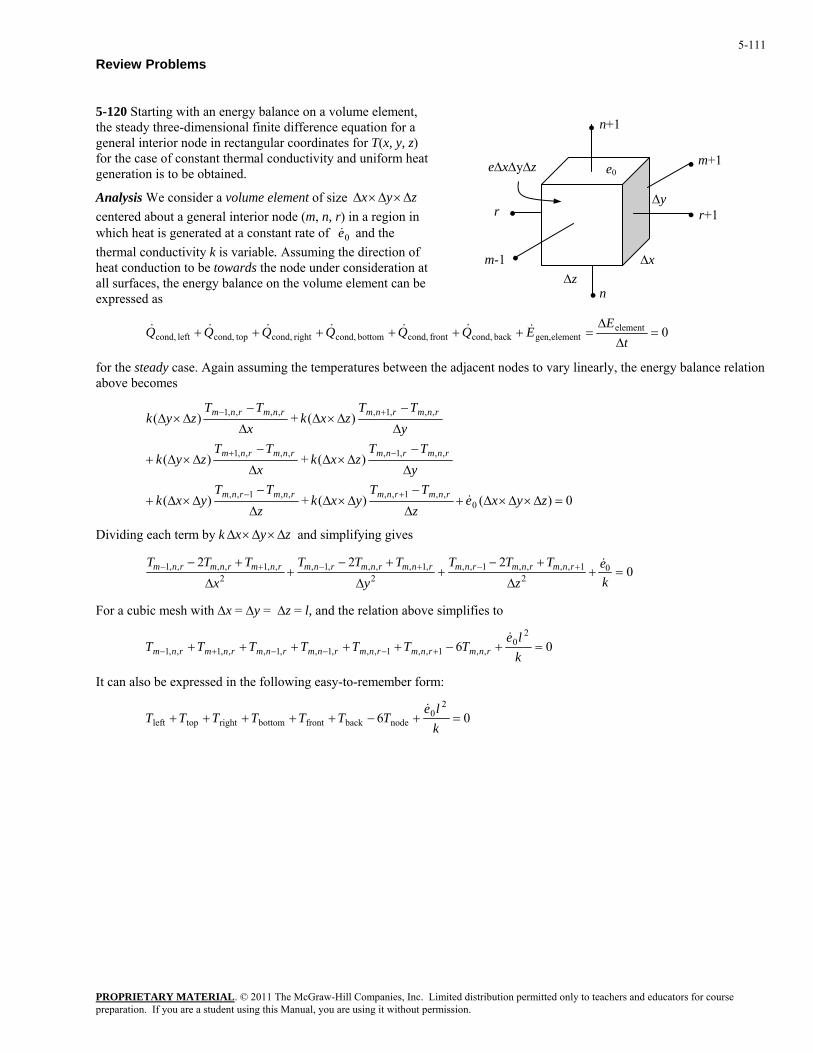
PROPRIETARY MATERIAL. © 2011 The McGraw-Hill Companies, Inc. Limited distribution permitted only to teachers and educators for course preparation. If you are a student using this Manual, you are using it without permission.
5-111
at
e element of size
Review Problems
5-120 Starting with an energy balance on a volume element, the steady three-dimensional finite difference equation for a n+1 general interior node in rectangular coordinates for T(x, y, z) for the case of constant thermal conductivity and uniform hegeneration is to be obtained.
Analysis We consider a volum zyx ∆×∆×∆ c (mentered about a general interior node , n, r) in a region in which heat is generated at a constant rate of and the
0e&thermal conductivity k is variable. Assuming the direction of heat conduction to be towards the node under consideration at all surfaces, the energy balance on the volume element can be expressed as
0elementelementgen,back cond,front left cond, cond,bottom cond,right cond, topcond, =
∆∆
=++++++t
EEQQQQQQ &&&&&&&
for the steady case. Again assuming the temperatures between the adjacent nodes to vary linearly, the energy balance relation above becomes
0)()(+ )( ∆×∆ yxk m
)(+ )( ,,,1,,,,,1 −∆×∆
∆
−∆×∆+ −+ TT
zxkx
TTzyk rnmrnmrnmrnm
)(+
0,,1,,,,1,,
,,,,,,,,1
=∆×∆×∆+∆
−∆×∆
∆
−+
∆
∆
−∆×∆
∆
−
+−
−
zyxez
TTyxk
zTT
y
yTT
zxkx
Tk
rnrnmrnmrnm
rnmrmrnmrnm
&
ng each term by and simplifying gives
)( 1∆×∆ +Tzy n
Dividi k zyx ∆×∆×∆
0222 0
21,,,,1,,
2,1,,,,1,
2,,1,,,,1 =+
∆
+−+
∆
+−+
∆
+− +−+−+
ke
zTTT
yTTT
xT rnmrnmrnmrnmrnmrnmrnmrnm &
w ∆x = ∆y = ∆z = l, and the relation above simplifies to
− rnm TT
For a cubic mesh ith
062
0,,1,,1,,,1,,1,,,1,,1− mrnm =+−+++++ +−−−+ k
leTTTTTTT rnmrnmrnmrnmrnmrn
&
can al ressed in the following easy-to-remember form: It so be exp
062
0nodebackfrontbottomrighttopleft =+−+++++
kle
TTTTTTT&
e∆x∆y∆z
•
•
•
•
••
n
r+1r
m+1
m-1
e0
∆z ∆x
∆y
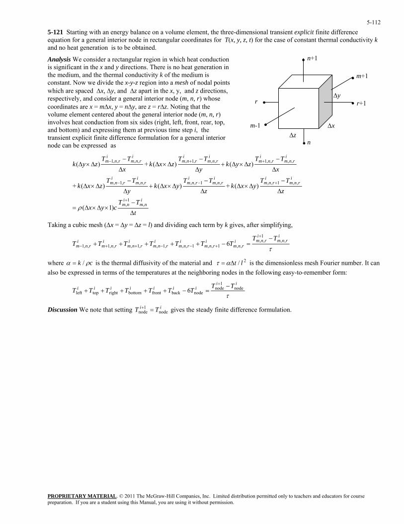
PROPRIETARY MATERIAL. © 2011 The McGraw-Hill Companies, Inc. Limited distribution permitted only to teachers and educators for course preparation. If you are a student using this Manual, you are using it without permission.
5-112
ance on a volume element, the three-dimensional transient explicit finite difference in rectangular coordinates for T(x, y, z, t) for the case of constant thermal conductivity k
nd no hea neration is to be obtained.
nalysis We consider a rectangular region in which heat conduction
l points ∆z apart in the x, y, and z directions, eneral interior node (m, n, r) whose
t centered about e general interior node (m, n, r)
ssed as
5-121 Starting with an energy balequation for a general interior node a t ge
A n+1 is significant in the x and y directions. There is no heat generation in the medium, and the thermal conductivity k of the medium is constant. Now we divide the x-y-z region into a mesh of nodawhich are spaced ∆x, ∆y, andrespectively, and consider a gcoordinates are x = m∆x, y = n∆y, are z = r∆z. Noting that the volume elemen thinvolves heat conduction from six sides (right, left, front, rear, top, and bottom) and expressing them at previous time step i, the transient explicit finite difference formulation for a general interior node can be expre
tTT
cyx
zTT
yxkz
TTyxk
yTT
zxk
xTT
zyky
TTzxk
xTT
zyk
inm
inm
irnm
irnm
irnm
irnm
irnm
irnm
irnm
irnm
irnm
irnm
irnm
irnm
∆
−×∆×∆=
∆
−∆×∆
∆
−∆×∆+
∆
−∆×∆
∆
−∆×∆+
∆
−∆×∆
∆
−∆×∆
+
+−−
++−
,1
,
,,1,,,,1,,,,,1,
,,,,1,,,1,,,,,1
)1(
)(+)()(+
)()(+)(
ρ
Taking a cubic mesh (∆x = ∆y = ∆z = l) and dividing each term by k gives, after simplifying,
τ
irnm
irnmi
rnmi
rnmi
rnmi
rnmi
rnmi
rnmi
rnmTT
TTTTTTT ,,1,,
,,1,,1,,,1,,1,,,1,,1 6−
=−++++++
+−−++−
where ck ρα /= is the thermal diffusivity of the material and is the dimensionless mesh Fourier number. It can also be expressed in terms of the temperatures at the neighboring nodes in the following easy-to-remember form:
2/ lt∆=ατ
τ
iiiiiiiii TT
TTTTTTT node1
nodenodebackfrontbottomrighttopleft 6
−=−+++++
+
Discussion We note that setting gives the steady finite difference formulation. ii TT node1
node =+
•
•
•
•
••
n
1
m+1
∆yr+r
m-1∆z
∆x
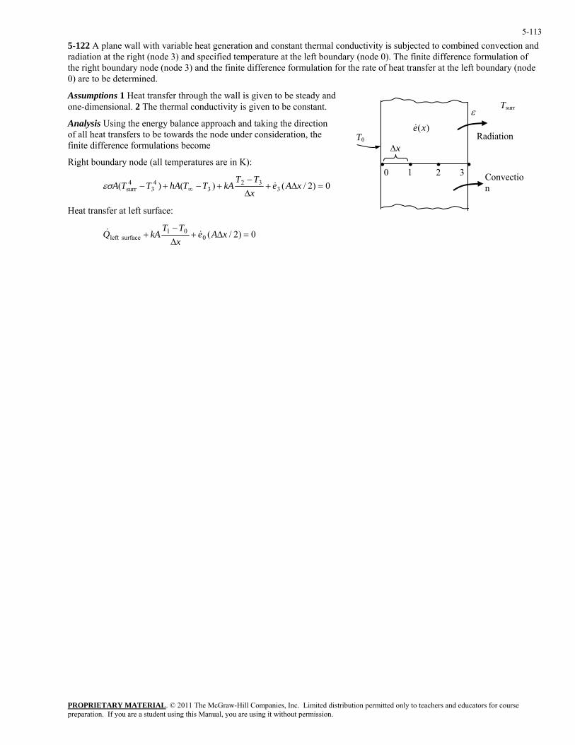
PROPRIETARY MATERIAL. © 2011 The McGraw-Hill Companies, Inc. Limited distribution permitted only to teachers and educators for course preparation. If you are a student using this Manual, you are using it without permission.
5-113
node (node 3) and the finite difference formulation for the rate of heat transfer at the left boundary (node
wall is given to be steady and onstant.
become
ight boundary node (all temperatures are in K):
5-122 A plane wall with variable heat generation and constant thermal conductivity is subjected to combined convection andradiation at the right (node 3) and specified temperature at the left boundary (node 0). The finite difference formulation of the right boundary0) are to be determined.
Assumptions 1 Heat transfer through the
Convection
∆xT0
• • • •0 1 2 3
Tsurr
Radiation
ε
)(xe&
one-dimensional. 2 The thermal conductivity is given to be c
Analysis Using the energy balance approach and taking the directionof all heat transfers to be towards the node under consideration, the finite difference formulations
R
0)2/()()( 332
34
34
surr =∆+∆−
+−+− ∞ xAexTT
kATThATTA &εσ
Heat transfer at left surface:
0)2/(001
surfaceleft =∆+∆
+ xAex
kAQ && −TT
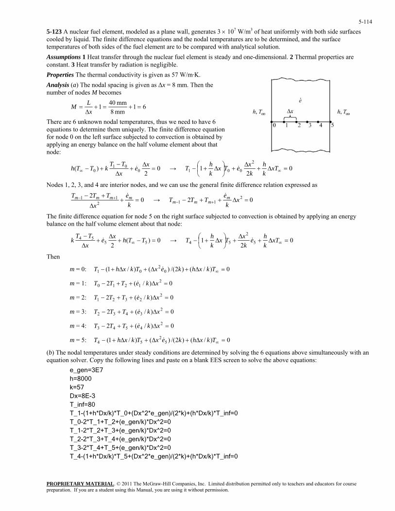
PROPRIETARY MATERIAL. © 2011 The McGraw-Hill Companies, Inc. Limited distribution permitted only to teachers and educators for course preparation. If you are a student using this Manual, you are using it without permission.
5-114
eat uniformly with both side surfaces nce equations and the nodal temperatures are to be determined, and the surface uel element are to be compared with analytical solution.
ssumptions 1 Heat transfer through the nuclear fuel element is steady and one-dimensional. 2 Thermal properties are onstant. 3 at transfer b d tion is negligible.
ies The thermal conductivity is given as 57 W/m·K.
5-123 A nuclear fuel element, modeled as a plane wall, generates 3 × 10⁷ W/m3 of hcooled by liquid. The finite differetemperatures of both sides of the fAc He y ra iaPropertAnalysis (a) The nodal spacing is given as ∆x = 8 mm. Then the number of nodes M becomes
61mm 8mm 401 =+=+
∆=
xLM
There are 6 unknown nodal temperatures, thus we need to have 6 equations to determine them uniquely. The finite difference equation for node 0 on t e lh eft surface subjected to convection is obtained by pplying an energy balance on the half volume element about that
node:
a
02
)( 001
0 =∆
+∆−
+−∞xe
xTT
kTTh & → 02
12
001 =∆+∆
+⎟⎠⎞
⎜⎝⎛ ∆+− ∞xT
kh
kxeTx
khT &
Nodes 1, 2, 3, and 4 are interior nodes, and we can use the general finite difference relation expressed as
02
211 =+
∆
+− +−
ke
xTTT mmmm &
→ 02 211 =∆++− +− x
ke
TTT mmmm
&
The finite difference equation for node 5 on the right surface subjected to convection is obtained by applying an energy balance on the half volume element about that node:
0)(2 55
54 =−+∆
+∆−
∞ TThxexTT
k & → 02
1 5
2
54 =∆+∆
+⎟⎠⎞
⎜⎝⎛ ∆+− ∞xT
khe
kxTx
khT &
Then
m = 0:
m = 1:
m = 2:
m = 3:
m = 4:
m = 5:
(b) The nodal temperatures under steady conditions are determined by solving the 6 equations above simultaneously with an equation solver. Copy the following lines and paste on a blank EES screen to solve the above equations: e_gen=3E7 h=8000 k=57 Dx=8E-3 T_inf=80 T_1-(1+h*Dx/k)*T_0+(Dx^2*e_gen)/(2*k)+(h*Dx/k)*T_inf=0 T_0-2*T_1+T_2+(e_gen/k)*Dx^2=0 T_1-2*T_2+T_3+(e_gen/k)*Dx^2=0 T_2-2*T_3+T_4+(e_gen/k)*Dx^2=0 T_3-2*T_4+T_5+(e_gen/k)*Dx^2=0 T_4-(1+h*Dx/k)*T_5+(Dx^2*e_gen)/(2*k)+(h*Dx/k)*T_inf=0
0)/()2/()()/1( 02
01 =∆+∆+∆+− ∞TkxhkexTkxhT &
0)/(2 21210 =∆++− xkeTTT &
0)/(2 22321 =∆++− xkeTTT &
0)/(2 23432 =∆++− xkeTTT &
0)/(2 24543 =∆++− xkeTTT &
0)/()2/()()/1( 52
54 =∆+∆+∆+− ∞TkxhkexTkxhT &
PROPRIETARY MATERIAL. © 2011 The McGraw-Hill Companies, Inc. Limited distribution permitted only to teachers and educators for course preparation. If you are a student using this Manual, you are using it without permission.
5-115
Solving by EES software, we get
C 155 °=0T , C 222 °=1T , C 256 °=2T
C 256 °=3T , C 222 °=4T , C 155 °=5T
(c) Using the analytical solution from Chapter 2, for a plane wall temperature exposed to convection can be determined using
of thickness 2L with heat generation, the surface
C 155 °=⋅
×+°=+=
W103(C 807
gen LeTT
&∞ W/m8000 2 wallplane , hs
The analytical solution matches exactly with the results obtained temperatures, C 155 °== TT .
K)m 02.0)(/m3
(for both sides)
using numerical method for both sides of the surface
ent are exposed to the same liquid temperature and convection heat transfer coefficient, it is possible to solve half of the plane wall by treating the centerline of the plane wall as symmetry line and get
50
Discussion Since both side of the fuel elem
the same results.
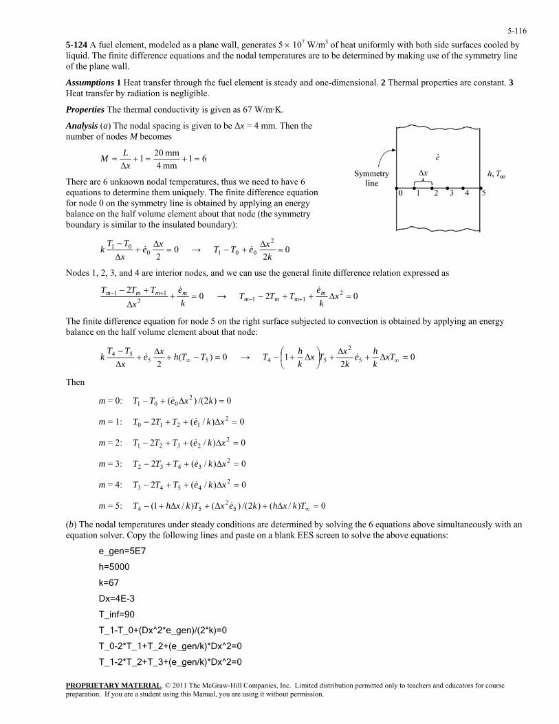
PROPRIETARY MATERIAL. © 2011 The McGraw-Hill Companies, Inc. Limited distribution permitted only to teachers and educators for course preparation. If you are a student using this Manual, you are using it without permission.
5-116
at uniformly with both side surfaces cooled by mined by making use of the symmetry line
2 Thermal properties are constant. 3
given to be ∆x = 4 mm. Then the omes
5-124 A fuel element, modeled as a plane wall, generates 5 × 10⁷ W/m3 of heliquid. The finite difference equations and the nodal temperatures are to be deterof the plane wall.
Assumptions 1 Heat transfer through the fuel element is steady and one-dimensional. Heat transfer by radiation is negligible.
Properties The thermal conductivity is given as 67 W/m·K.
Analysis (a) The nodal spacing isnumber of nodes M bec
61mm 4mm 201 =+=+
∆=
xLM
There are 6 unknown nodal temequations to determine
peratures, thus we need to have 6 them uniquely. The finite difference equation
ode 0 the symmetry line is obtained by applying an energy e element about that node (the symmetry
ry is similar
for n onbalance on the half volumbounda to the insulated boundary):
020
01 =∆
+∆− xexTT
k & → 02
2
001 =∆
+−kxeTT &
Nodes 1, 2, 3, and 4 are interior nodes, and we can use the general finite difference relation expressed as
02
211 =+
∆
+− +−
ke
xTTT mmmm &
→ 02 211 =∆++− +− x
ke
TTT mmmm
&
The finite difference equation for node 5 on the right surface subjected to convection is obtained by applying an energy balance on the half volume element about that node:
0)(2 55
54 =−+∆
+∆−
∞ TThxexTT
k & → 02
1 5
2
54 =∆+∆
+⎟⎠⎞
⎜⎝⎛ ∆+− ∞xT
khe
kxTx
khT &
Then
m = 0:
m = 1:
m = 2:
m = 3:
m = 4:
m = 5:
(b) The nodal temperatures under steady conditions are determined by solving the 6 equations above simultaneously with an equation solver. Copy the following lines and paste on a blank EES screen to solve the above equations:
e_gen=5E7
h=5000
k=67
Dx=4E-3
T_inf=90
T_1-T_0+(Dx^2*e_gen)/(2*k)=0
T_0-2*T_1+T_2+(e_gen/k)*Dx^2=0
T_1-2*T_2+T_3+(e_gen/k)*Dx^2=0
0)2/()( 2001 =∆+− kxeTT &
0)/(2 21210 =∆++− xkeTTT &
0)/(2 22321 =∆++− xkeTTT &
0)/(2 23432 =∆++− xkeTTT &
0)/(2 24543 =∆++− xkeTTT &
0)/()2/()()/1( 52
54 =∆+∆+∆+− ∞TkxhkexTkxhT &
PROPRIETARY MATERIAL. © 2011 The McGraw-Hill Companies, Inc. Limited distribution permitted only to teachers and educators for course preparation. If you are a student using this Manual, you are using it without permission.
5-117
T_4-(1+h*Dx/k)*T_5+(Dx^2*e_gen)/(2*k)+(h*Dx/k)*T_inf=0
,
T_2-2*T_3+T_4+(e_gen/k)*Dx^2=0
T_3-2*T_4+T_5+(e_gen/k)*Dx^2=0
Solving by EES software, we get
C 439 °=0T , C 433 °=1T , C 415 °=2T
C 386 °=3T , =4T C 290 ° C 344 ° =5T
Discussion Using the analytical solution from Chapter 2, for a plane wall of thickness 2L with heat generation, the surfatemperature exposed to convection can be determined using
ce
C290K W/m5000
C 90 2 wallplane , °=⋅
+°=+= ∞ h
TTs )m 02.0)( W/m105( 37gen ×Le&
The analytical solution matches exactly with the results obtained using numerical method for both sides of the surface temperatures, C2905 °= T .
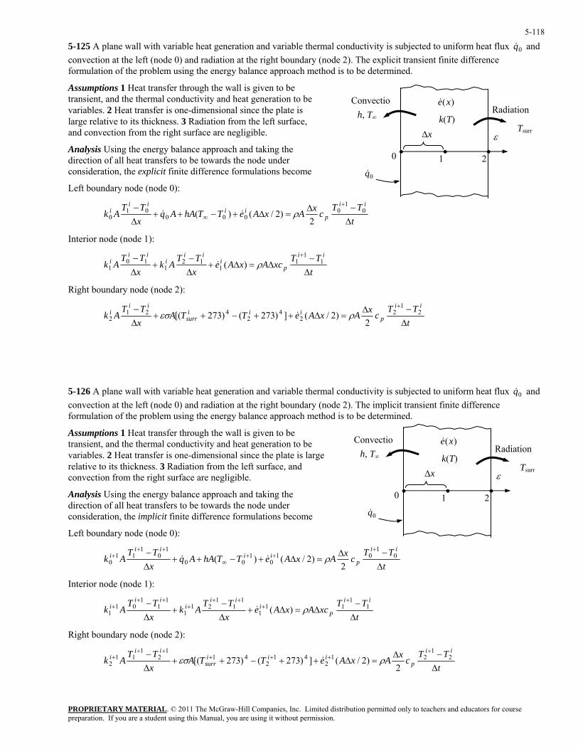
PROPRIETARY MATERIAL. © 2011 The McGraw-Hill Companies, Inc. Limited distribution permitted only to teachers and educators for course preparation. If you are a student using this Manual, you are using it without permission.
5-118
nd
at transfer through the wall is given to be
t
n, the explicit
5-125 A plane wall with variable heat generation and variable thermal conductivity is subjected to uniform heat flux 0q& aconvection at the left (node 0) and radiation at the right boundary (node 2). The explicit transient finite difference formulation of the problem using the energy balance approach method is to be determined.
Assumptions 1 Hetransient, and the thermal conductivity and heat generation to be variables. 2 Heat transfer is one-dimensional since the plate is large relative to its thickness. 3 Radiation from the left surface, and convection from he right surface are negligible.
Analysis Using the energy balance approach and taking the direction of all heat transfers to be towards the node under consideratio finite difference formulations become
Left boundary node (node 0):
tp ∆∞ 000 2)2/()(
TTcxAxAeTThAAq
xTT
Aki
iiii
i −∆=∆+−++
∆− +
01
0010 ρ&&
terior no (node 1):
i
In de
tTT
cAeTT
AkTT
Akii
pi
iii
iii −
+−
+− +
11
11
121
101 (& xAx
xx ∆∆=∆
∆∆) ρ
Right boundary node (node 2):
t
TTcxAxAeTTA
x∆ 2TT
Akii
piii
surr
iii
∆−∆
=∆++−++− +
21
22
42
4212 )2/(])273()273[( ρεσ &
5-126 A plane wall with variable heat generation and variable thermal conductivity is subjected to uniform heat flux and convection at the left (node 0) and radiation at the right boundary (node 2). The implicit transient finite difference formulation of the problem using the energy balance approach method is to be determined.
Assumptions 1 Heat transfer through the wall is given to be transient, and the thermal conductivity and heat generation to be variables. 2 Heat transfer is one-dimensional since the plate is large relative to its thickness. 3 Radiation from the left surface, and convection from the right surface are negligible.
Analysis Using the energy balance approach and taking the direction of all heat transfers to be towards the node under consideration, the implicit finite difference formulations become
Left boundary node (node 0):
&q0
tTT
cxAxAeTThAAqxTT
Akii
pii
iii
∆−∆
=∆+−++∆− +
++∞
+++ 0
101
01
00
10
111
0 2)2/()( ρ&&
Interior node (node 1):
tTT
xcAxAexTT
AkxTT
Akii
pi
iii
iii
∆−
∆=∆+∆−
+∆− +
+++
+++
+ 11
111
11
121
1
11
101
1 )( ρ&
Right boundary node (node 2):
t
TTcxAxAeTTA
xTT
Akii
piii
surr
iii
∆−∆
=∆++−++∆− +
+++++
+ 21
212
412
411
21
112 2
)2/(])273()273[( ρεσ &
Convectio
∆x
1
ε
Convectio
∆x
1
ε• ••0 2
Tsurr
Radiationh, T∞ k(T)
)(xe&
0q&
Tsurr
Radiation h, T∞ k(T)
)(xe&
0q&
• ••0 2
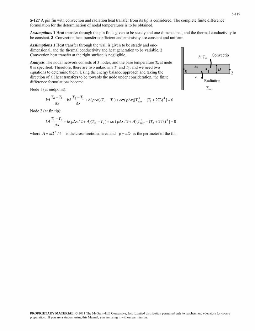
PROPRIETARY MATERIAL. © 2011 The McGraw-Hill Companies, Inc. Limited distribution permitted only to teachers and educators for course preparation. If you are a student using this Manual, you are using it without permission.
5-119
to
at transfer at the right surface is negligible.
ature T0 at node we need two
ance approach and taking the ration, the finite
5-127 A pin fin with convection and radiation heat transfer from its tip is considered. The complete finite difference formulation for the determination of nodal temperatures is to be obtained.
Assumptions 1 Heat transfer through the pin fin is given to be steady and one-dimensional, and the thermal conductivitybe constant. 2 Convection heat transfer coefficient and emissivity are constant and uniform.
Assumptions 1 Heat transfer through the wall is given to be steady and one-dimensional, and the thermal conductivity and heat generation to be variable. 2 Convection he Convectio
h, T∞
• ••0 1 2D∆x
Tsurr
Radiationε
Analysis The nodal network consists of 3 nodes, and the base temper0 is specified. Therefore, there are two unknowns T1 and T2, andequations to determine them. Using the energy baldirection of all heat transfers to be towards the node under considedifference formulations become
Node 1 (at midpoint):
0])273()[())(( 11210 ∆+−∆+
∆−
+∆−
∞ xpTTxphxTT
kAxTT
kA εσ 41
4surr =+− TT
ode 2 (at fin tip): N
0])273()[2/( ∆+εσ))(2/( 42
4surr2
21 =+−+−+∆+∆−
∞ TTAxpTTAxphxTT
kA
where 4/2DA π= is the cross-sectional area and Dp π= is the perimeter of the fin.
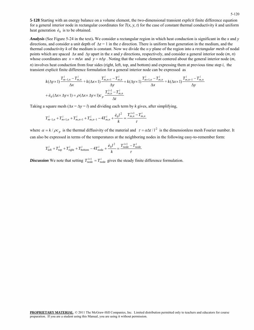
PROPRIETARY MATERIAL. © 2011 The McGraw-Hill Companies, Inc. Limited distribution permitted only to teachers and educators for course preparation. If you are a student using this Manual, you are using it without permission.
5-120
rm
and y
ates are and . Noting that the volume element centered about the general interior node (m, xpressing them at previous time step i, the
n be expressed as
5-128 Starting with an energy balance on a volume element, the two-dimensional transient explicit finite difference equation for a general interior node in rectangular coordinates for T(x, y, t) for the case of constant thermal conductivity k and unifoheat generation 0e& is to be obtained.
Analysis (See Figure 5-24 in the text). We consider a rectangular region in which heat conduction is significant in the x directions, and consider a unit depth of ∆z = 1 in the z direction. There is uniform heat generation in the medium, and thethermal conductivity k of the medium is constant. Now we divide the x-y plane of the region into a rectangular mesh of nodal points which are spaced ∆x and ∆y apart in the x and y directions, respectively, and consider a general interior node (m, n) whose coordin xmx ∆= yny ∆=n) involves heat conduction from four sides (right, left, top, and bottom) and etransient explicit finite difference formulation for a general interior node ca
tTT
cyxyxe
TTyk
yTT
xkTT
yk
inm
inm
p
inm
inm
inm
inm
inm
∆
−×∆×∆=×∆×∆+
∆
−×∆+
∆
−×∆
−×∆
+
++−
,1
,0
,1,1,,,1
)1()1(
)1()1(+)1(
ρ&
yTT
xkxx
inm
inm
inm
∆
−×∆
∆− ,1,, )1(+
ng a sq re mesh (∆x = ∆y = l) and dividing each term by k gives, after simplifying, Taki ua
τ
inm
inmi
nmi
nmi
nmi
nmi
nmTT
kle
TTTTT ,1
,2
0,1,1,,1,1 4
−=+−+++
+
−++−&
where pck ρα /= is the thermal diffusivity of the material and 2/ lt∆=ατ is the dimensionless mesh Fourier number. It ca en also be xpressed in terms of the temperatures at the neighboring nodes in the following easy-to-remember form:
τ
iiiii T
TTT node1
node −+++
ii Tkle
TT2
0nodebottomrighttopleft 4 =+−+
&
Discussion gives the steady finite difference formulation. ii TT node1
node =+ We note that setting
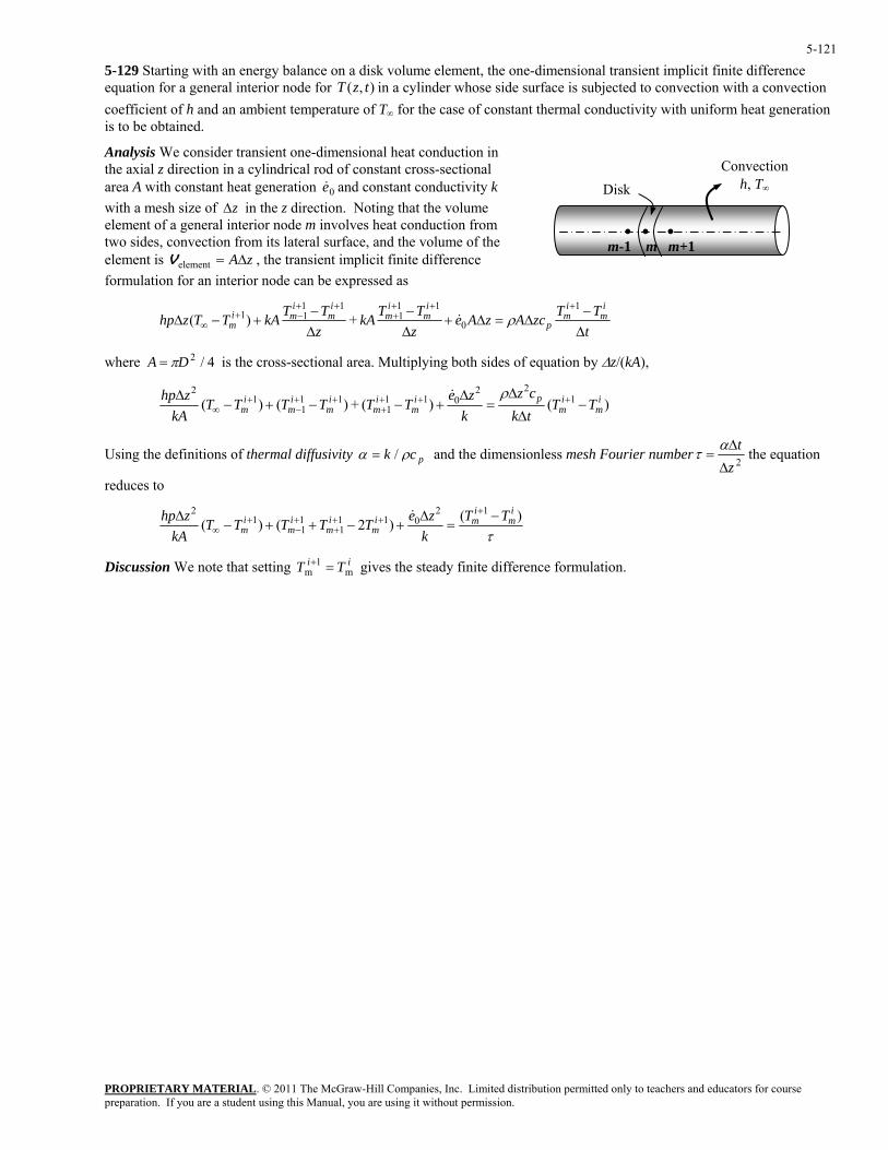
PROPRIETARY MATERIAL. © 2011 The McGraw-Hill Companies, Inc. Limited distribution permitted only to teachers and educators for course preparation. If you are a student using this Manual, you are using it without permission.
5-121
s subjected to convection with a convection al conductivity with uniform heat generation
heat conduction in on in a cylindrical rod of constant cross-sectional
stant conductivity k
5-129 Starting with an energy balance on a disk volume element, the one-dimensional transient implicit finite difference equation for a general interior node for ),( tzT in a cylinder whose side surface icoefficient of h and an ambient temperature of T∞ for the case of constant thermis to be obtained.
Analysis We consider transient one-dimensionalthe axial z directi
• • • m-1 m m+1
Convectionh, T∞Disk area A with constant heat generation 0e& and con
with a mesh size of z∆ in the z direction. Notingelement of a general interior node
that the volume m involves heat conduction from
o sides, convecti om its lateral surface, and the volume of the lement is , the transient implicit finite difference rmulation for an interior
twe
on frzA∆=elementV
fo node can be expressed as
tTTzcAzAe
zTTkA
zTTkATTzhp
im
im
p
im
im
im
imi
m ∆−
∆=∆+∆−
∆−
+−∆+++
+++
−+∞
1
0
111
1111 +)( ρ&
where is the cross-sectional area. Multiplying both sides of equation by ∆z/(kA),
4/2DA π=
)()(+)()( 122
0111
111
12
im
im
pim
im
im
im
im TT
tkcz
kzeTTTTTT
kAzhp
−∆
∆=
∆+−−+−
∆ ++++
++−
+∞
ρ&
pck ρα /= and the dimensionless mesh Fourier number2zt
∆
∆=ατUsing the definitions of thermal diffusivity the equation
reduces to
τ)()2()(
12011
111
12 i
mi
mim
im
im
im
TTk
zeTTTTTkA
zhp −=
∆+−++−
∆ +++
++−
+∞
&
Discussion We note that setting gives the steady finite difference formulation. ii TT m1
m =+
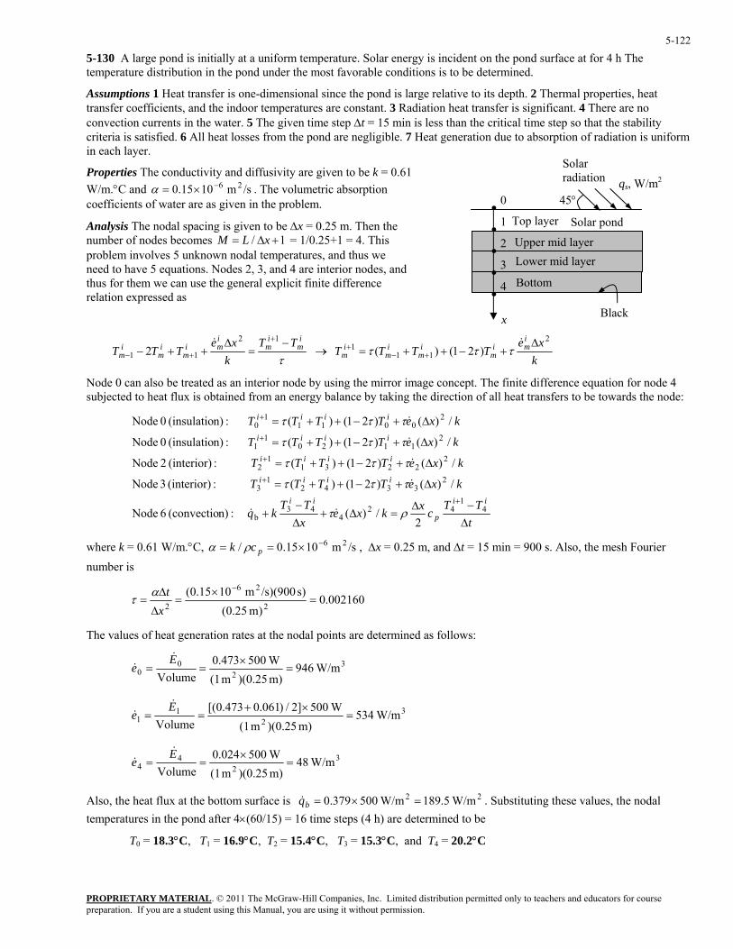
PROPRIETARY MATERIAL. © 2011 The McGraw-Hill Companies, Inc. Limited distribution permitted only to teachers and educators for course preparation. If you are a student using this Manual, you are using it without permission.
5-122
perties, heat
lity uniform
roperties The conductivity and diffusivity are given to be k = 0.61 /m.°C and . The volumetric absorption
oefficients of water are as given in the problem.
nalysis The nodal spacing is given to be ∆x = 0.25 m. Then the ber of nodes become = 1/0.25+1 = 4. This
roblem involves 5 unknown nodal temperatures, and thus we eed to have 5 equations. Nodes 2, 3, and 4 are interior nodes, and us for them we can use the general explicit finite difference lation expressed as
5-130 A large pond is initially at a uniform temperature. Solar energy is incident on the pond surface at for 4 h The temperature distribution in the pond under the most favorable conditions is to be determined.
Assumptions 1 Heat transfer is one-dimensional since the pond is large relative to its depth. 2 Thermal protransfer coefficients, and the indoor temperatures are constant. 3 Radiation heat transfer is significant. 4 There are no convection currents in the water. 5 The given time step ∆t = 15 min is less than the critical time step so that the stabicriteria is satisfied. 6 All heat losses from the pond are negligible. 7 Heat generation due to absorption of radiation isin each layer.
qs, W/m2
Solar radiation
x
Top layer
45°
Solar pond
Black
• • • • •
0 1 2 3 4
Upper mid layerLower mid layer
Bottom
P/sm 1015.0 26−×=αW
c
As 1/ +∆= xLMnum
pnthre
τ
im
im
imi
mi
mi
mTT
kxe
TTT−
=∆
++−+
+−
12
11 2&
→ k
xeTTTT
imi
mi
mi
mi
m
2
111 )21()(
∆+−++= +−
+ &τττ
Node 0 can also be treated as an interior node by using the mirror image concept. The finite difference equation for node 4 subjec ea btain n energy balance by taking the direction of all heat transfers to be towards the node:
ted to h t flux is o ed from a
tTT
cxkxexTT
kq &
kxeTTT
kxeTTT
kxeTTT
kxeTTT
ii
p
ii
iii
iiii
iii
iiii
∆−∆
=∆+∆−
+
∆+−++=
∆+−++=
∆+−++=
∆+−++=
+
+
+
41
424
43b
23342
22231
12
211201
20011
1
2/)(:n)nvectio6 Node
/)()21()( :rior)3 Node
/)()21()( :erior)2 Node
/)()21()( :n)ulatio0 Node
/)()21()( :n)atio0 Node
ρτ
τττ
τττ
τττ
τττ
&
&
&
&
&
= 0.61 W/m.°C, , ∆x = 0.25 m, and ∆t = 15 min = 900 s. Also, the mesh Fourier
T i+13
T
T
T i+1
0
(co
(inte
(int
(ins
(ins ul
/sm 1015.0/ 26−×== pck ραwhere k number is
002160.0)m 25.0(
s) /s)(900m 1015.0(2
26
2=
×=
∆
∆=
−
xtατ
The values of heat generation rates at the nodal points are determined as follows:
32
00 W/m946
m) )(0.25m (1 W500473.0
Volume=
×==
Ee
&&
32
11 W/m534
m) )(0.25m (1 W500]2/)061.0473.0[(
Volume=
×+==
Ee
&&
32
44 W/m48
m) )(0.25m (1 W500024.0
Volume=
×==
Ee
&&
Also, the heat flux at the bottom surface is . Substituting these values, the nodal temperatures in the pond after 4×(60/15) = 16 time steps (4 h) are determined to be
T0 = 18.3°C, T1 = 16.9°C, T2 = 15.4°C, T3 = 15.3°C, and T4 = 20.2°C
22 W/m5.189 W/m500379.0 =×=bq&
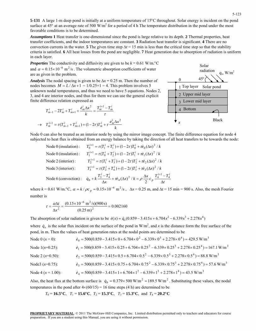
PROPRIETARY MATERIAL. © 2011 The McGraw-Hill Companies, Inc. Limited distribution permitted only to teachers and educators for course preparation. If you are a student using this Manual, you are using it without permission.
5-123
temperature of 15°C throughout. Solar energy is incident on the pond rface at 4 ° at an average rate of 500 W/m2 for a period of 4 h The temperature distribution in the pond under the most vorable c nditions is to be determined.
t transfer is one-dimensional since the pond is large relative to its depth. 2 Thermal properties, heat transfer coefficients, and the indoor temperatures are constant. 3 Radiation heat transfer is significant. 4 There are no onvection currents in the water. 5 The given time step t = 15 min is less than the critical time step so that the stability
criteria is satisfied. 6 All heat losses from the pond are negligible. 7 Heat generation due to absorption of radiation is uniform
are given to be k = 0.61 W/m.°C nd . The volumetric absorption coefficients of water
. Analysis The nodal spacing is given to be ∆x = 0.25 m. Then the number of odes become = 1/0.25+1 = 4. This problem involves 5
peratures, and thus we need to have 5 equations. Nodes 2, 3, and 4 are interior nodes, and thus for them we can use the general explicit
xpressed as
5-131 A large 1-m deep pond is initially at a uniformsu 5fa oAssumptions 1 Hea
c ∆
in each layer. Properties The conductivity and diffusivity
qs, W/m2
Solar radiation
x
Top layer
45°
Solar pond
Black
• • • • •
0 1 2 3 4
Upper mid layerLower mid layer
Bottom
/sm 1015.0 26−×=αaare as given in the problem
nunknown nodal tem
s 1/ +∆= xLM
finite difference relation e
τ
im
im
imi
mi
mi m
TTk
xeTTT
−=
∆++−
+
+−
12
11 2&
→ k
xeTTTT
imi
mi
mi
mi
m
2
111 )21()(
∆+−++= +−
+ &τττ
Node 0 can also be treated as an interior node by using the mirror image concept. The finite difference equation for node 4 subjected to heat flux is obtained from an energy balance by taking the direction of all heat transfers to be towards the node:
tTT
cxkxexTT
kq
kxeTTTT
kxeTTTT
kxeTTTT
kxeTTTT
ii
p
ii
b
iiii
iiii
iiii
iiii
∆−∆
=∆+∆−
+
∆+−++=
∆+−++=
∆+−++=
∆+−++=
+
+
+
+
+
41
424
43
23342
13
22231
12
21120
11
20011
10
2/)( :n)(convectio 6 Node
/)()21()( :(interior) 3 Node
/)()21()( :(interior) 2 Node
/)()21()( :n)(insulatio 0 Node
/)()21()( :n)(insulatio 0 Node
ρτ
τττ
τττ
τττ
τττ
&&
&
&
&
&
where k = 0.61 W/m.°C, , ∆x = 0.25 m, and ∆t = 15 min = 900 s. Also, the mesh Fourier number is
/sm 1015.0/ 26−×== pck ρα
002160.0)m 25.0(
s) /s)(900m 1015.0(2
26
2=
×=
∆
∆=
−
xtατ
The absorption of solar radiation is given to be
where is the solar flux incident on the surface of the pond in W/m2, and x is the distance form the free surface of the pond, in m. Then the values of heat generation rates at the nodal points are determined to be
Node 0 (x = 0):
Node 1(x=0.25):
Node 2 (x=0.50):
Node3 (x=0.75):
Node 4 (x = 1.00):
Also, the heat flux at the bottom surface is . Substituting these values, the nodal temperatures in the pond after 4×(60/15) = 16 time steps (4 h) are determined to be
T0 = 16.5°C, T1 = 15.6°C, T2 = 15.3°C, T3 = 15.3°C, and T4 = 20.2°C
)278.2339.6704.6415.3859.0()( 432 xxxxqxe s +−+−= &&
sq&
34320 W/m5.429)0278.20339.60704.60415.3859.0(500 =×+×−×+×−=e&
34321 W/m1.167)25.0278.225.0339.625.0704.625.0415.3859.0(500 =×+×−×+×−=e&
34322 W/m8.88)5.0278.25.0339.65.0704.65.0415.3859.0(500 =×+×−×+×−=e&
34323 W/m6.57)75.0278.275.0339.675.0704.675.0415.3859.0(500 =×+×−×+×−=e&
34324 W/m5.43)1278.21339.61704.61415.3859.0(500 =×+×−×+×−=e&
22 W/m5.189 W/m500379.0 =×=bq&
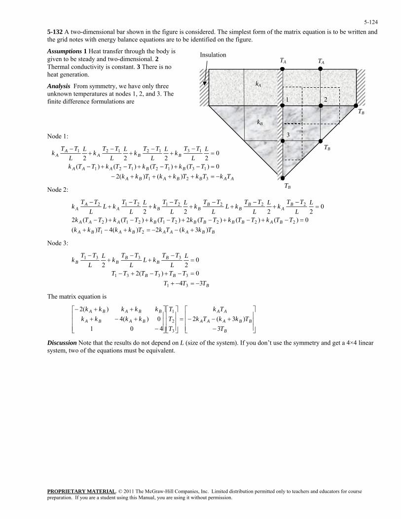
PROPRIETARY MATERIAL. © 2011 The McGraw-Hill Companies, Inc. Limited distribution permitted only to teachers and educators for course preparation. If you are a student using this Manual, you are using it without permission.
5-124
d
.
Node 1:
5-132 A two-dimensional bar shown in the figure is considered. The simplest form of the matrix equation is to be written anthe grid notes with energy balance equations are to be identified on the figure.
Assumptions 1 Heat transfer through the body is given to be steady and two-dimensional. 2 Thermal conductivity is constant. 3 There is no heat generation
Insulation
Analysis From symmetry, we have only three unknown temperatures at nodes 1, 2, and 3. The finite difference formulations are
AABBABA
BB
BBA
A
TkTkTkkTkTTkTTkTk
LL
TTkL
LTTT
k
−=++++=−+−+
=−
+−
+
321
13121
1312
)()0)()()
022
Node 2:
TB
kB
kA
1
3
2
TB
TB
TA TA
AAA
kTkTT
−−+− 21
(2()(
A kLL
TTkL
LT −
+− 121
22
BBAAABABA
BABBBBBA
AA
TkkTkTkkTkTTkT
LTT
k
)3(2)(40()
21
22221212
2
+−−=+−+
−
Node 3:
AA
BA
BB
BBBA
kkTTkTTkTTTTkTk
LL
TTkL
LTT
kLL
TTkL
LTT
kLL
TTkL
)()()()(2)()(2
02222
2222121
+=−+−+−+−+−−
=−
+−
+−
+−
+−
+
B
BB
TTTTTTTTT
340)(2
31
3331
−=−+=−+−+−
BB
BBB L
kLL
kL
k 022
3331 =++LTTTTLTT −−−
The matrix equation is
Discussion Note that the results do not depend on L (size of the system). If you don’t use the symmetry and get a 4×4 linear system, two of the equations must be equivalent.
⎥⎥⎥
⎦
⎤
⎢⎢⎢
⎣
⎡
−+−−=
⎥⎥⎥
⎦
⎤
⎢⎢⎢
⎣
⎡
⎥⎥⎥
⎦
⎤
⎢⎢⎢
⎣
⎡
−+−+
++−
B
BBAAA
AA
BABA
BBABA
TTkkTk
Tk
TTT
kkkkkkkkk
3)3(2
4010)(4
)(2
3
2
1
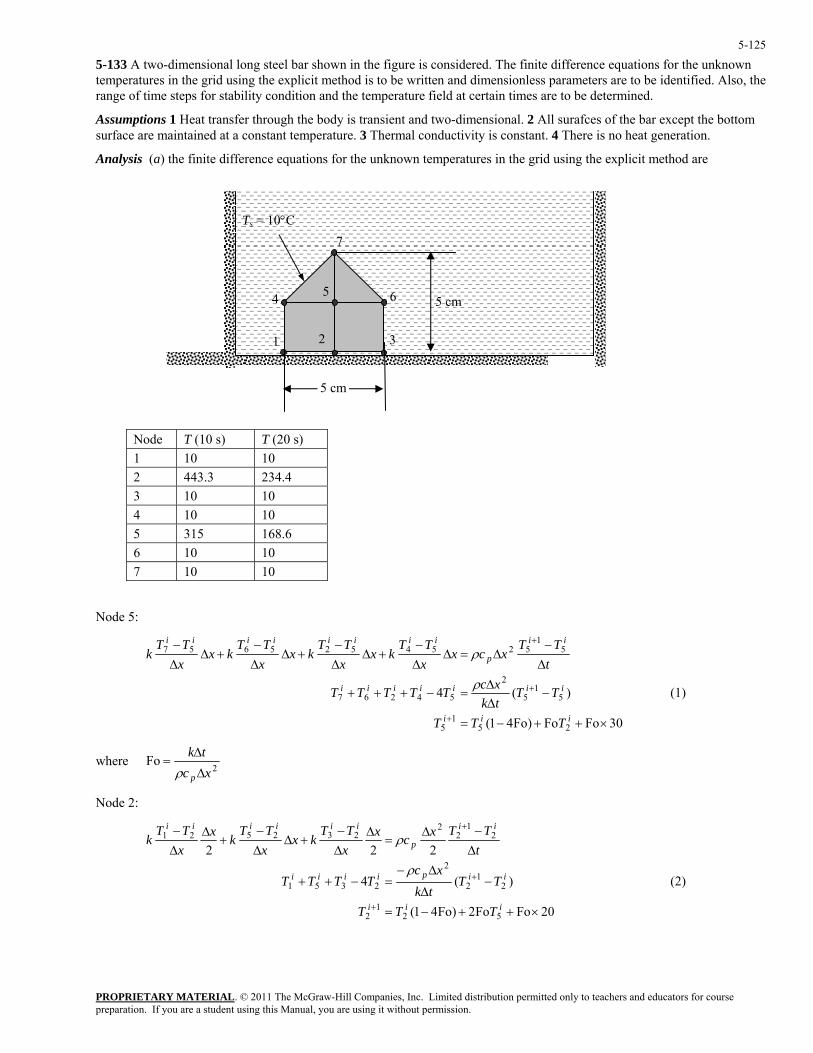
PROPRIETARY MATERIAL. © 2011 The McGraw-Hill Companies, Inc. Limited distribution permitted only to teachers and educators for course preparation. If you are a student using this Manual, you are using it without permission.
5-125
e steps for stability condition and the temperature field at certain times are to be determined.
nsional. 2 All surafces of the bar except the bottom is constant. 4 There is no heat generation.
the unknown temperatures in the grid using the explicit method are
Node T (10 s) T (20 s)
5-133 A two-dimensional long steel bar shown in the figure is considered. The finite difference equations for the unknown temperatures in the grid using the explicit method is to be written and dimensionless parameters are to be identified. Also, thrange of time
Assumptions 1 Heat transfer through the body is transient and two-dimesurface are maintained at a constant temperature. 3 Thermal conductivity
Analysis (a) the finite difference equations for
Ts = 10°C
1 10 10 2 443.3 234.4 3 10 10 4 10 10 5 315 168.6 6 10 10 7 10 10
Node 5:
30FoFo)Fo41(
)(4
251
5
51
5
2
54267
51
5254525657
×++−=
−∆∆
=−+++
∆−
∆=∆∆−
+∆∆−
+∆∆−
+∆∆−
+
+
+
iii
iiiiiii
ii
p
iiiiiiii
TTT
TTtkxcTTTTT
tTT
xcxxTT
kxxTT
kxxTT
kxxTT
k
ρ
ρ
(1)
where 2
Foxctk
p∆
∆=ρ
Node 2:
20FoFo2)Fo41(
)(4
222
521
2
21
2
2
2351
21
22
232521
×++−=
−∆
∆−=−++
∆−∆
=∆
∆−
+∆∆−
+∆
∆−
+
+
+
iii
iipiiii
ii
p
iiiiii
TTT
TTtk
xcTTTT
tTTxcx
xTT
kxxTT
kxxTT
k
ρ
ρ
(2)
1 8 3
6 5 4
7
5 cm 5
2
5 cm
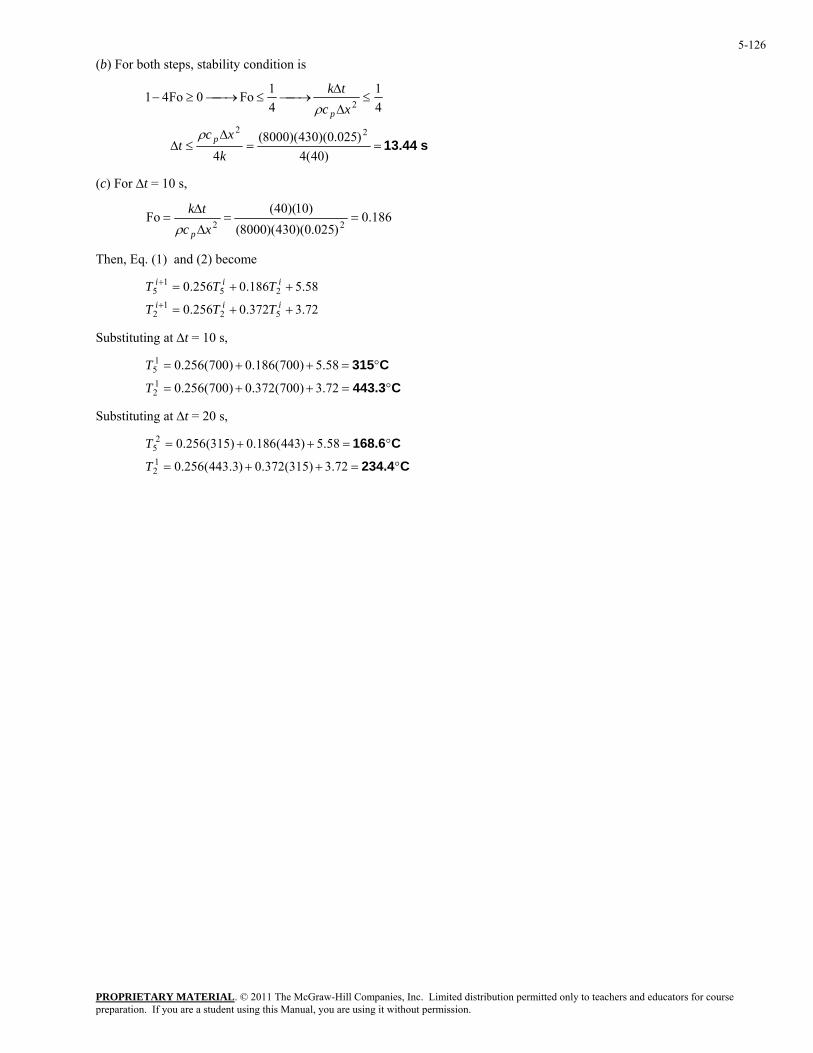
PROPRIETARY MATERIAL. © 2011 The McGraw-Hill Companies, Inc. Limited distribution permitted only to teachers and educators for course preparation. If you are a student using this Manual, you are using it without permission.
5-126
(b) For both steps, stability condition is
s 13.44==∆
≤∆
≤∆
∆⎯→⎯≤⎯→⎯≥−
)40(4)025.0)(430)(8000(
4
44Fo0Fo41
22
2
kxc
t
xc
p
p
ρ
ρ
(c) For ∆t = 10 s,
11 tk
186.0 )025.0)(430)(8000(
)10)(40(Fo2
==∆
∆=
xctk
pρ
Then, Eq. (1) and (2) become
58.5186.0256.0
125
15 ++=+
+
iii
iii TTT
2
522 ++= TTT
Substituting at ∆t = 10 s,
°=++= 58.5)700(186.0)700(256.01
5T
°=++ 58.5)443(186.0)315(256T
72.3372.0256.0
C315
C443.3°=++= 72.3)700(372.0)700(256.012T
Substituting at ∆t = 20 s,
= .02
5 C168.6
C234.4°=++= 72.3)315(372.0)3.443(256.012T
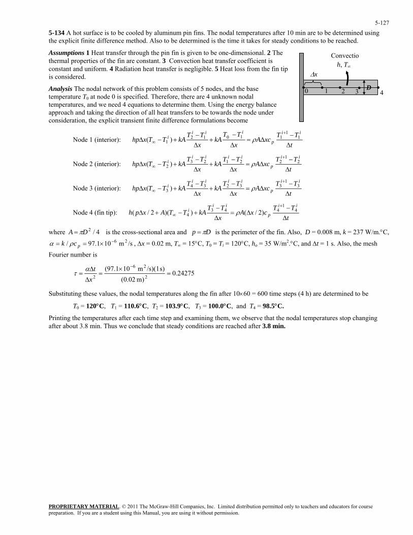
PROPRIETARY MATERIAL. © 2011 The McGraw-Hill Companies, Inc. Limited distribution permitted only to teachers and educators for course preparation. If you are a student using this Manual, you are using it without permission.
5-127
hot surface is to be cooled by aluminum pin fins. The nodal tem tthe explicit finite difference method. Also to be determined is the time it takes for steady conditions to be reached.
ransfer through the pin fi ven t . 2 The
iatio sfer is nis considered.
temperat al temperat gy balance approach and taking the direction of all heat transfers to be towards the node under consideration, the explicit transient finite difference formulations become
5-134 A peratures after 10 min are to be de ermined using
Assumptions 1 Heat t n is gi o be one-dimensional Convectio
thermal properties of the fin are constant. 3 Convection heat transfer coefficient is constant and uniform. 4 Rad n heat tran egligible. 5 Heat loss from the fin tip h, T∞
• •4
•0 2 D
∆x
• •31Analysis The nodal network of this problem consists of 5 nodes, and the base ure T0 at node 0 is specified. Therefore, there are 4 unknown nodures, and we need 4 equations to determine them. Using the ener
Node 1 (interior): t
xcAx
kAx
kATTxhp pi
∆∆=
∆+
∆+−∆ ∞
1110121 )( ρ
TTTTTT iiiii −−− +1
Node 2 (interior): t
TTxcA
xTT
kAxTT
kATTxhpii
p
iiiii
∆−
∆=∆−
+∆−
+−∆+
∞2
122123
2 )( ρ
tTT
xcAxTT
kAxTT
kATTxhpii
p
iiiii
∆−
∆=∆−
+∆−
+−∆+
∞3
133234
3 )( ρ Node 3 (interior):
Node 4 (fin tip): t
cxAx
kATTAxph pi
∆∆=
∆+−+∆ ∞
44434 )2/())(2/( ρ
where 4/2DA π=
TTTT iiii −− +1
is the cross-sectional area and Dp π= is the perimeter of the fin. Also, D = 0.008 m, k = 237 W/m.°C, 6−== pck ρα °C, T0 = Ti = 120°C, ho = 35 W/m2.°C, and ∆t = 1 s. Also, the mesh
Fourier number is
/sm 101 2× , ∆x = 0.02 m, T∞ = 15.97/
24275.0)m 02.0(
s) /s)(1m 101.97(2
26
2=
×=
∆
∆=
−
xtατ
Substituting these values, the nodal temperatures along the fin after 10×60 = 600 time steps (4 h) are determined to be
T0 = 120°C, T1 = 110.6°C, T2 = 103.9°C, T3 = 100.0°C, and T4 = 98.5°C.
Printing the temperatures after each time step and examining them, we observe that the nodal temperatures stop changing after about 3.8 min. Thus we conclude that steady conditions are reached after 3.8 min.
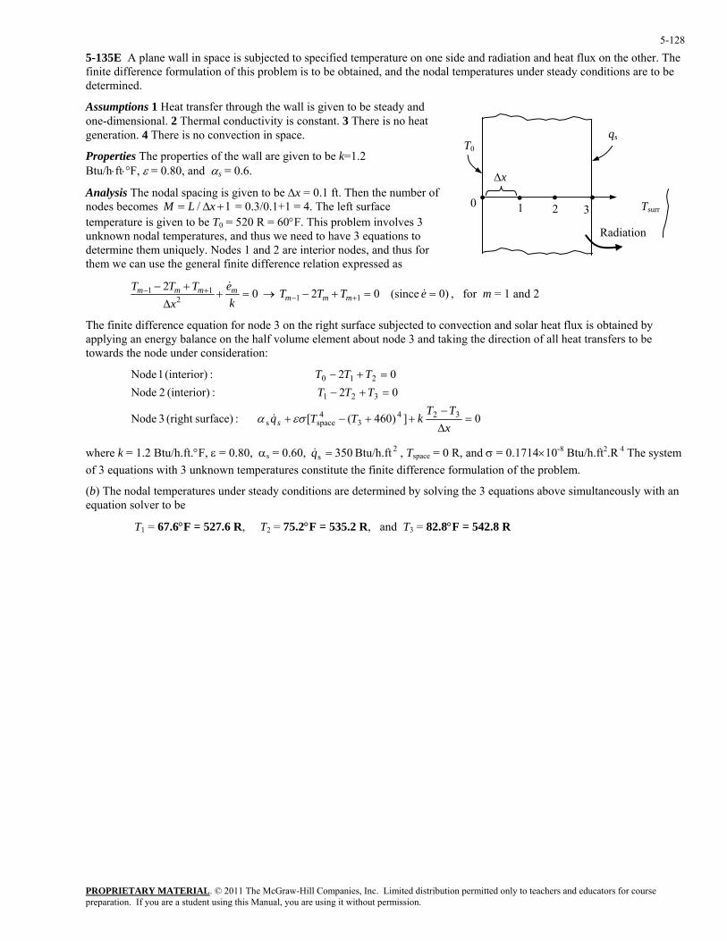
PROPRIETARY MATERIAL. © 2011 The McGraw-Hill Companies, Inc. Limited distribution permitted only to teachers and educators for course preparation. If you are a student using this Manual, you are using it without permission.
5-128
itions are to be
he number of ce
ves 3 s, and thus we need have 3 equations to
determine them uniqu and thus for ressed as
5-135E A plane wall in space is subjected to specified temperature on one side and radiation and heat flux on the other. The finite difference formulation of this problem is to be obtained, and the nodal temperatures under steady conddetermined.
Assumptions 1 Heat transfer through the wall is given to be steady and one-dimensional. 2 Thermal conductivity is constant. 3 There is no heat generation. 4 There is no convection in space.
Properties The properties of the wall are given to be k=1.2 Btu/h⋅ft⋅°F, ε = 0.80, and αs = 0.6.
qsT0
Analysis The nodal spacing is given to be ∆x = 0.1 ft. Then tnodes becomes 1/ +∆= xLM = 0.3/0.1+1 = 4. The left surfatemperature is given to be T0 = 520 R = 60°F. This problem involunknown nodal temperature to
ely. Nodes 1 and 2 are interior nodes, them we can use the general finite difference relation exp
)0 (since 02 021 −− TT mm112
1 ==+−→=+∆
++−
+ eTTTk
ex
Tmmm
mm &&
, for m = 1 and 2
The finite difference equation for node 3 on the right surface subjected to convection and solar heat flux is obtained by applying an energy balance on the half volume element about node 3 and taking the direction of all heat transfers to be towards the node under consideration:
0])460([ :surface)(right 3 Node 3243
4spaces =
∆−
++−+
0 :(interior) 2 Node02 :(interior) 1 Node
321
210
=2 +−=+−
xTT
kTTqs εσα &
TTTTT
where k = 1.2 Btu/h.ft.°F, ε = 0.80, αs = 0.60, Tspace = 0 R, and σ = 0.1714×10⁻⁸ Btu/h.ft2.R 4 The system s with 3 unknown temperatures constitute the finite difference formulation of the problem.
(b The nodal temperatures under steady conditions are determined by solving the 3 equations above simultaneously with an equation solver to be
T1 = 67.6°F = 527.6 R, T2 = 75.2°F = 535.2 R, and T3 = 82.8°F = 542.8 R
•
∆x
Radiation
1• ••0 2 3 Tsurr
T
2s Btu/h.ft 350=q& ,
of 3 equation
)
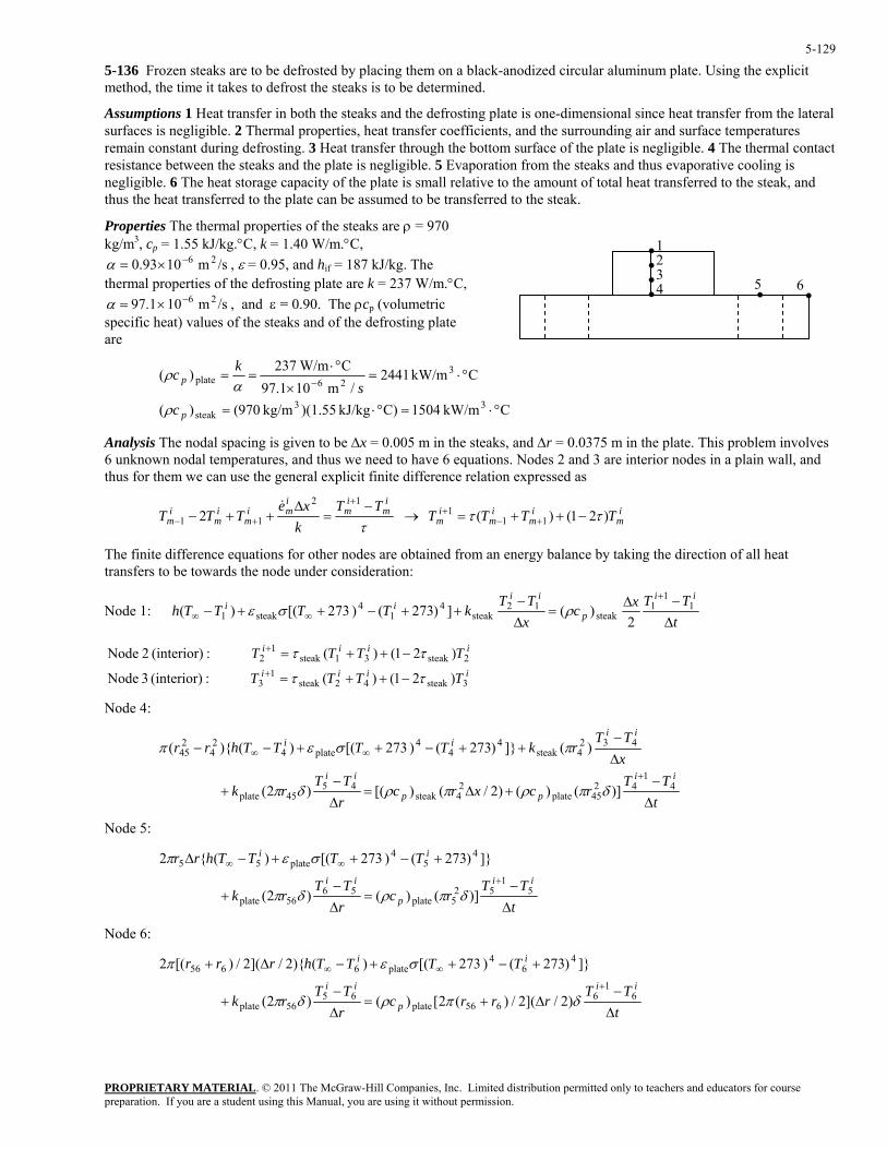
PROPRIETARY MATERIAL. © 2011 The McGraw-Hill Companies, Inc. Limited distribution permitted only to teachers and educators for course preparation. If you are a student using this Manual, you are using it without permission.
5-129
F lacing them on a black-a takes to defrost the steaks is to be determined.
eral
remain constant during defrosting. 3 Heat transfer through the bottom surface of the plate is negligible. 4 The thermal contact resistance between the steaks and the plate is negligible Evaporation from the steaks and thus evaporative cooling is negligible. 6 The heat storage capacity of the plate is small relative to the amount of total heat transferred to the steak, and
p
ε = 0.95, and hif = 187 kJ/kg. The he defrosting plate are k = 237 W/m.°C, , and ε = 0.90. The ρcp (volumetric
eaks and of the defrosting plate
5-136 rozen steaks are to be defrosted by p nodized circular aluminum plate. Using he explicit method, the time it t
Assumptions 1 Heat transfer in both the steaks and the defrosting plate is one-dimensional since heat transfer from the latsurfaces is negligible. 2 Thermal properties, heat transfer coefficients, and the surrounding air and surface temperatures
. 5
thus the heat transferred to the plate can be assumed to be transferred to the steak.
Properties The thermal properties of the steaks are ρ = 970 kg/m3, c = 1.55 kJ/kg.°C, k = 1.40 W/m.°C,
5
• • •
12 3 4 ••
6/sm 1093.0 26−×=α ,
thermal properties of t/sm 101.97 26−×=α
specific heat) values of the st
•
are
CkW/m 1504C)kJ/kg )(1.55kg/m 970()( 33steak °⋅=°⋅=pcρ
Analysis The nodal spacing is given to be ∆x = 0.005 m in the steaks, and ∆r = 0.0375 m in the plate. This problem involves
CkW/m 2441/m 101.97
)(26plate °⋅=
×==
−psα
6 unknown nodal t m eratures, and t o have 6 equations. Nodes 2 and 3 are interior nodes in a plain wall, and thus for t licit finite difference relation expressed as
C W/m237 3°⋅kcρ
e p hus we need them we can use the general exp
τ
im
im
imi
mi
mi
mTT
kxe
TTT−
=∆
++−+
+−
12
11 2&
→
The finite difference equations for other nodes are obtained from an energy balance by taking the direction of all heat transfers to be towards the node under consideration:
Node 1:
im
im
im
im TTTT )21()( 11
1 ττ −++= +−+
tTTxc
xTT
kTTTThii
p
iiii
∆−∆
=∆−
++−++−+
∞∞1
11
steak12
steak4
14
steak1 2)(])273() 273[()( ρσε
iiii
iiii
TTTT
TTTT
3steak42steak1
3
2steak31steak1
2
)21()( :(interior) 3 Node
)21()( :(interior) 2 Node
ττ
ττ
−++=
−++=+
+
Node 4:
tTT
rcxrcrTT
rk
xTT
rkTTTThrr
ii
pp
ii
iiii
∆−
+∆=∆−
+
∆−
++−++−−
+
∞∞
41
4245plate
24steak
4545plate
4324steak
44
4plate4
24
245
)]()()2/()[()2(
)(]})273() 273[()(){(
δπρπρδπ
πσεπ
Node 5:
tTT
rcrTT
rk
TTTThrrii
p
ii
ii
∆−
=∆−
+
+−++−∆+
∞∞
51
525plate
5656plate
45
4plate55
)]()()2(
]})273() 273[()({2
δπρδπ
σεπ
Node 6:
tTT
rrrcrTT
rk
TTTThrrrii
p
ii
ii
∆−
∆+=∆−
+
+−++−∆++
∞∞
61
6656plate
6556plate
46
4plate6656
)2/](2/)(2[)()2(
]})273() 273[()(){2/](2/)[(2
δπρδπ
σεπ
PROPRIETARY MATERIAL. © 2011 The McGraw-Hill Companies, Inc. Limited distribution permitted only to teachers and educators for course preparation. If you are a student using this Manual, you are using it without permission.
5-130
×= , and εplate = 0.90, T∞ = 20°C,
where C,kW/m 1504)( C,kW/m 2441)( 3steak
3plate °⋅=°⋅= pp cc ρρ ksteak = 1.40 W/m.°C, , εsteak = 0.95,
/sm 1093.0 26steak
−×=α , hif = 187 kJ/kg, kplate = 237 W/m.°C, 26plate
−α /sm 101.97
h =12 W/m2.°C, δ = 0.01 m, ∆x = 0.005 m, ∆r = 0.0375 m, and ∆t = 5 s. Also, the mesh Fourier number for the steaks is
186.0)m 005.0( 22steak ==
∆=
xτ
s) /s)(5m 1093.0( 26×∆ −tα
The vari i are ous radi r4 =0.075 m, r5 =0.1125 m, r6 =0.15 m, r45 = (0.075+0.1125)/2 m, and r = (0.1125+0.15)/2 m.
The total amount of heat transfer needed to defrost the steaks is
πV
akifsteaklatentsensible
°°=
56
kg 257.0)]m 015.0(m) (0.075)[kg/m 970( 23steak === ρm
kJ 55.2=kJ/kg) kg)(187 257.0(+C)](-18-C)[0kJ/kg. kg)(1.55 257.0(
)()( stesteak total, +∆=+= mhTmcQQ p
The amount of heat transfer to the steak during a time step i is the sum of the heat transferred to the steak directly from its p surfa irectly through the plate, and is expressed as
]})273() 273[()(){(
]})273() 273[()(){2/](2/)[(2
]})273() 273[()({
41
4steak1
44
4plate4
24
245
46
4plate6656
45
4plate5
+−++−
+−++−−
+−++−∆++
+−++−∆=
∞∞
∞∞
∞∞
∞∞
ii
ii
ii
iii
TTTThr
TTTThrr
TTTThrrr
TTTThrr
σεπ
σεπ
σεπ
σεπ
ined by finding the amount of heat transfer during each time step, and adding them up until we 5.2 ultiplying the number of time steps N by the time step ∆t = 5 s will give the defrosting time. In this case it is
∆tdefrost = N∆t = 44(5 s) = 220 s
Q
to ce, and ind
2 5steakQ
+
21+ ]})273() 273[()({
The defrosting time is determobtain 5 kJ. Mdetermined to be
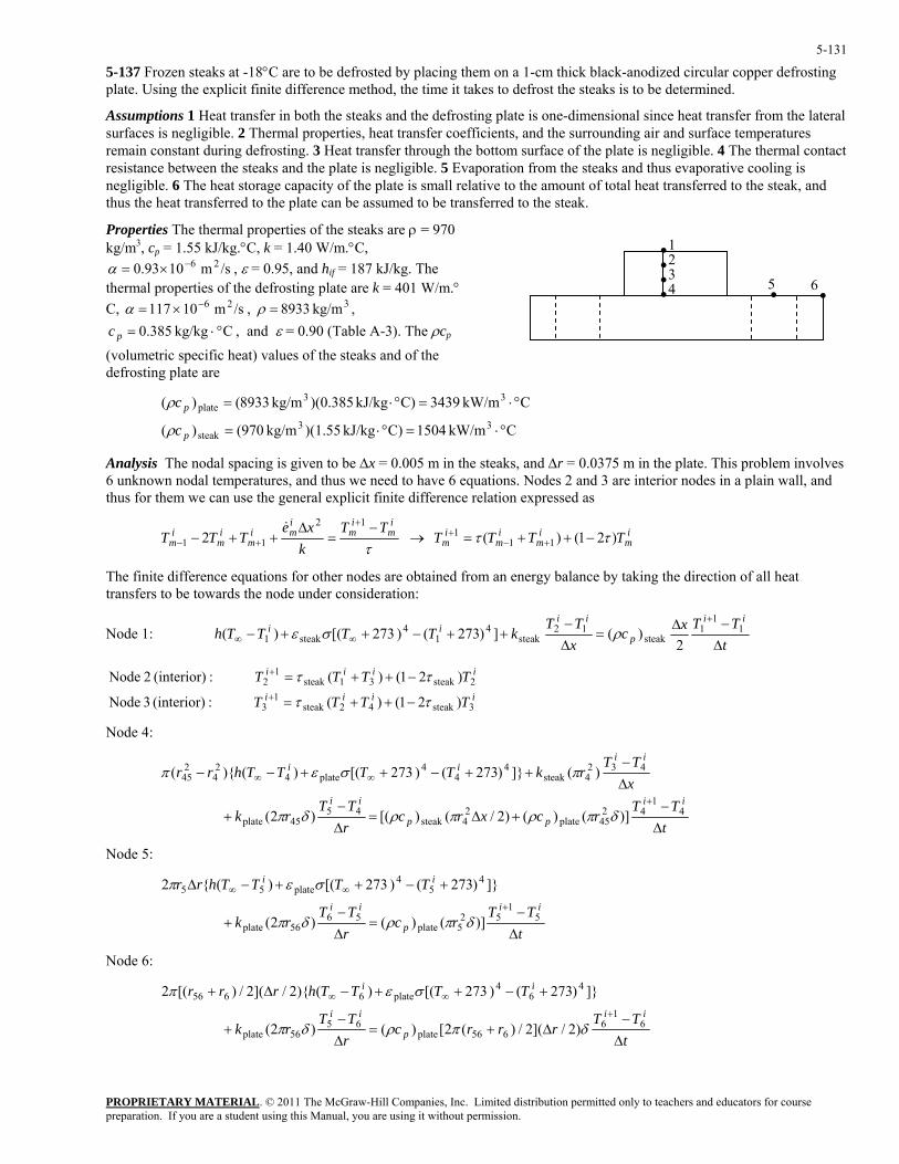
PROPRIETARY MATERIAL. © 2011 The McGraw-Hill Companies, Inc. Limited distribution permitted only to teachers and educators for course preparation. If you are a student using this Manual, you are using it without permission.
5-131
defrosting
at transfer in both the steaks and the defrosting plate is one-dimensional since heat transfer from the lateral ts, and the surrounding air and surface temperatures m surface of the plate is negligible. 4 The thermal contact
an be assumed to be transferred to the steak.
roperties The thermal properties of the steaks are ρ = 970 kg 3, cp = 1.55 kJ/kg.°C, k = 1.40 W/m.°C,
ε = 0.95, and hif = 187 kJ/kg. The ermal properties of the defrosting plate are k = 401 W/m.°
e A-3). The ρcp
(volumetric specific heat) values of the steaks and of the defrosting plate are
Analysis The nodal spacing is given to be ∆x = 0.005 m in the steaks, and ∆r = 0.0375 m in the plate. This problem involves 6 unknown nodal temperatures, and thus we need to have 6 equations. Nodes 2 and 3 are interior nodes in a plain wall, and thus for them we can use the general explicit finite difference relation expressed as
5-137 Frozen steaks at -18°C are to be defrosted by placing them on a 1-cm thick black-anodized circular copper plate. Using the explicit finite difference method, the time it takes to defrost the steaks is to be determined.
Assumptions 1 Hesurfaces is negligible. 2 Thermal properties, heat transfer coefficienremain constant during defrosting. 3 Heat transfer through the bottoresistance between the steaks and the plate is negligible. 5 Evaporation from the steaks and thus evaporative cooling is negligible. 6 The heat storage capacity of the plate is small relative to the amount of total heat transferred to the steak, and thus the heat transferred to the plate c
P/m
5
• • • •
12 3 4 ••
6/sm 1093.0 26−×=α ,
thC, /sm 10117 26−×=α , 3kg/m 8933=ρ ,
Ckg/kg 385.0 °⋅=pc , and ε = 0.90 (Tabl
CkW/m 1504C)kJ/kg )(1.55kg/m 970()(
CkW/m 3439C)kJ/kg )(0.385kg/m 8933()(33
steak
33plate
°⋅=°⋅=
°⋅=°⋅=
p
p
c
c
ρ
ρ
τ
im
im
imi
mi
mi
mTT
kxe
TTT−
=∆
++−+
+−
12
11 2&
→
The finite difference equations for other nodes are obtained from an energy balance by taking the direction of all heat transfers to be towards the node under consideration:
Node 1:
im
im
im
im TTTT )21()( 11
1 ττ −++= +−+
tTTxc
xTT
kTTTThii
p
iiii
∆−∆
=∆−
++−++−+
∞∞1
11
steak12
steak4
14
steak1 2)(])273() 273[()( ρσε
iiii
iiii
TTTT
TTTT
3steak42steak1
3
2steak31steak1
2
)21()( :(interior) 3 Node
)21()( :(interior) 2 Node
ττ
ττ
−++=
−++=+
+
Node 4:
tTT
rcxrcrTT
rk
xTT
rkTTTThrr
ii
pp
ii
iiii
∆−
+∆=∆−
+
∆−
++−++−−
+
∞∞
41
4245plate
24steak
4545plate
4324steak
44
4plate4
24
245
)]()()2/()[()2(
)(]})273() 273[()(){(
δπρπρδπ
πσεπ
Node 5:
tTT
rcrTT
rk
TTTThrrii
p
ii
ii
∆−
=∆−
+
+−++−∆+
∞∞
51
525plate
5656plate
45
4plate55
)]()()2(
]})273() 273[()({2
δπρδπ
σεπ
Node 6:
tTT
rrrcrTT
rk
TTTThrrrii
p
ii
ii
∆−
∆+=∆−
+
+−++−∆++
∞∞
61
6656plate
6556plate
46
4plate6656
)2/](2/)(2[)()2(
]})273() 273[()(){2/](2/)[(2
δπρδπ
σεπ
PROPRIETARY MATERIAL. © 2011 The McGraw-Hill Companies, Inc. Limited distribution permitted only to teachers and educators for course preparation. If you are a student using this Manual, you are using it without permission.
5-132
here ksteak = 1.40 W/m.°C, εsteak = 0.95,
hif = 187 kJ/kg, kplate = 401 W/m.°C, , and εplate = 0.90, T∞ = 20°C,
h =12 W/m2.°C, δ = 0.01 m, ∆x = 0.005 m, ∆r = 0.0375 m, and ∆t = 5 s. Also, the mesh Fourier number for the steaks is
w C,kW/m 1504)( C,kW/m 3439)( 3steak
3plate °⋅=°⋅= pp cc ρρ
/sm 1093.0 26steak
−×=α , /sm 10117 26plate
−×=α
186.0)m 005.0(
s) /s)(5m 1093.0(2
26
2steak =×
=∆
∆=
−
xtατ
The various radii are r4 =0.075 m, r5 =0.1125 m, r6 =0.15 m, r45 = (0.075+0.1125)/2 m, and r56 = (0.1125+0.15)/2 m.
The total amount of heat transfer needed to defrost the steaks is
kg 257.0)]m 015.0(m) (0.075)[kg/m 970( 23steak === πρVm
kJ 55.2=kJ/kg) kg)(187 257.0(+C)](-18-C)[0kJ/kg. kg)(1.55 257.0(
)()( steakifsteaklatentsensiblesteak total,
°°=
+∆=+= mhTmcQQQ p
The amount of heat transfer to the steak during a time step i is the sum of the heat transferred to the steak directly from its top surface, and indirectly through the plate, and is expressed as
]})273() 273[(
]})273() 273[()(){2/](2/)[(2
]})273() 273[()({2
41
44
4
46
4plate6656
45
4plate55steak
+
+−+
+−++−∆++
+−++−∆=
∞
∞∞
∞∞
i
i
ii
iii
TT
TTTThrrr
TTTThrrQ
σ
σεπ
σεπ
we btain 55.2 kJ. Multiplying the number of time steps N by the time step ∆t = 5 s will give the defrosting time. In this case it is etermined to be
∆tdefrost = N∆t = 47(5 s) = 235 s
)(){( plate42
42
45 +−−+ ∞iTThrr επ
() 273[()({ 4steak1
21 −++−+ ∞∞
i TTTThr σεπ ]})273
The defrosting time is determined by finding the amount of heat transfer during each time step, and adding them up until od
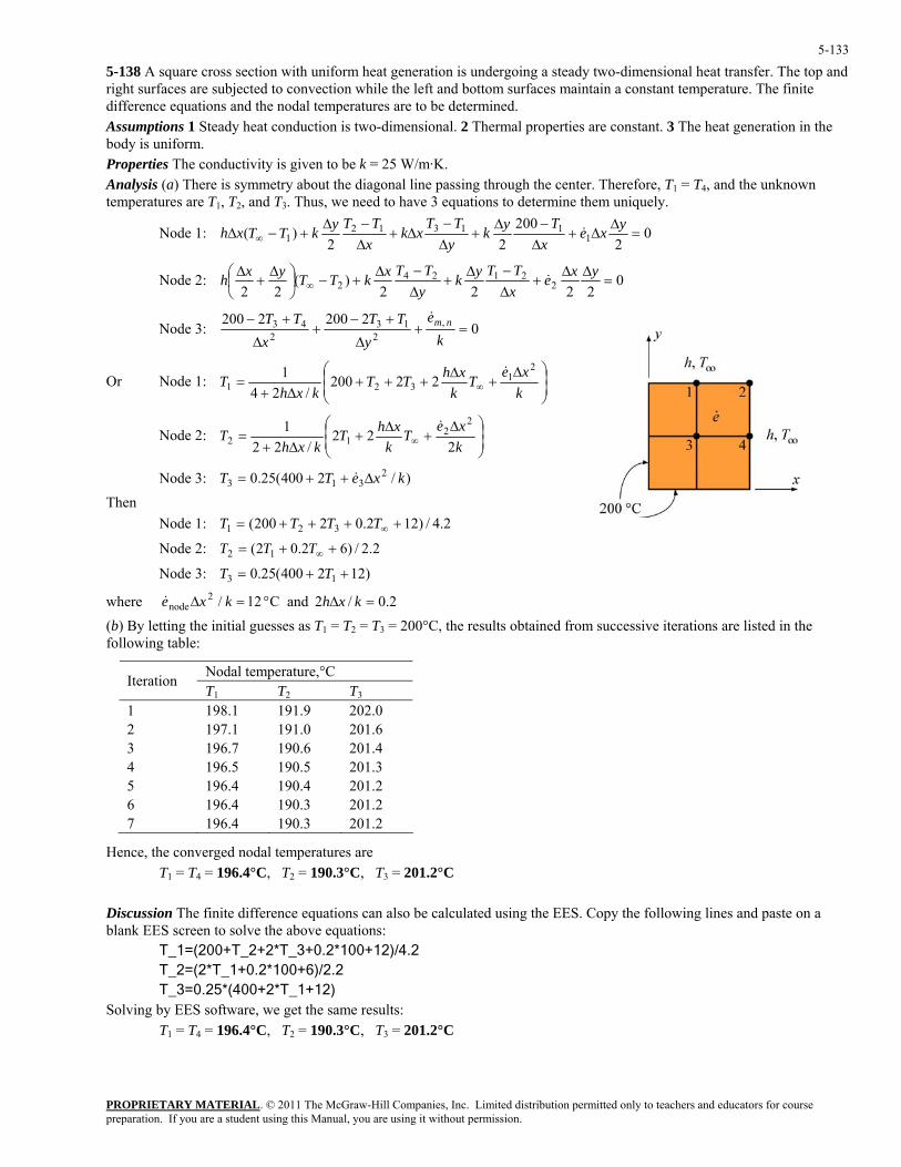
PROPRIETARY MATERIAL. © 2011 The McGraw-Hill Companies, Inc. Limited distribution permitted only to teachers and educators for course preparation. If you are a student using this Manual, you are using it without permission.
5-133
d
etermined.
s are T1, T2, and T3. Thus, we need to have 3 equations to determine them uniquely.
5-138 A square cross section with uniform heat generation is undergoing a steady two-dimensional heat transfer. The top anright surfaces are subjected to convection while the left and bottom surfaces maintain a constant temperature. The finite difference equations and the nodal temperatures are to be dAssumptions 1 Steady heat conduction is two-dimensional. 2 Thermal properties are constant. 3 The heat generation in the body is uniform. Properties The conductivity is given to be k = 25 W/m·K. Analysis (a) There is symmetry about the diagonal line passing through the center. Therefore, T1 = T4, and the unknown temperature
Node 1: 02
20022
)( 13121 ∆
−∆+
∆−
∆+∆−∆
+−∆ ∞ xyk
yTT
xkxTTykTTxh
Node 2:
11 =
∆∆+
yxeT
&
02222
)(22
1242 +
∆−∆
+∆−∆
+−⎟⎠⎞
⎜⎝⎛ ∆
+∆
∞ xTyk
yTTxkTTyxh
Node 3:
22 =
∆∆ yxeT
&
022002200
243 +−+
+− eTTTT & ,2
13 =+∆∆ kyx
nm
Or Node 1: ⎟⎟⎠
⎞⎜⎜⎝
⎛ ∆+
∆+++
∆+= ∞ k
xeT
kxhTT
kxhT
21
321 22200/24
1 &
Node 2: ⎟⎟⎠
⎞⎜⎜⎝
⎛ ∆+
∆+
∆+= ∞ k
xeT
kxhT
kxhT
222
/221 2
212
&
)/2400(25.0 2313 kxeTT ∆++= &
Then
Node 3:
Node 1: 2.4/)122.02200( 321 ++++= ∞TTTT
Node 2: 2.2/)62.02( 12 ++= ∞TTT
Node 3:
here °=k and
b) By lettin itial guesses as T1 = T2 = T3 = 200°C, the results obtained from successive iterations are listed in the llowin
dal temperature,°C
)122400(25.0 13 ++= TT
w /2node∆xe& C 12 2.0/2 =∆ kxh
( g the info g table:
NoIteration T2 T3T1
1 198.1 191.9 202.0 2 197.1 191.0 201.6 3 196.7 190.6 201.4
196.5 190.5 201.3 5 4
196.4 190.4 201.2 6 196.4 190.3 201.2 7 196.4 190.3 201.2
Hence, the converged nodal temperatures are T1 = T4 = 196.4°C, T2 = 190.3°C, T3 = 201.2°C
Discussion The finite difference equations can also be calculated using the EES. Copy the following lines and paste on a
T_3=0.25*(400+2*T_1+12) Solving by EES software, we get the same results: T1 = T4 = 196.4°C, T2 = 190.3°C, T3 = 201.2°C
blank EES screen to solve the above equations: T_1=(200+T_2+2*T_3+0.2*100+12)/4.2 T_2=(2*T_1+0.2*100+6)/2.2
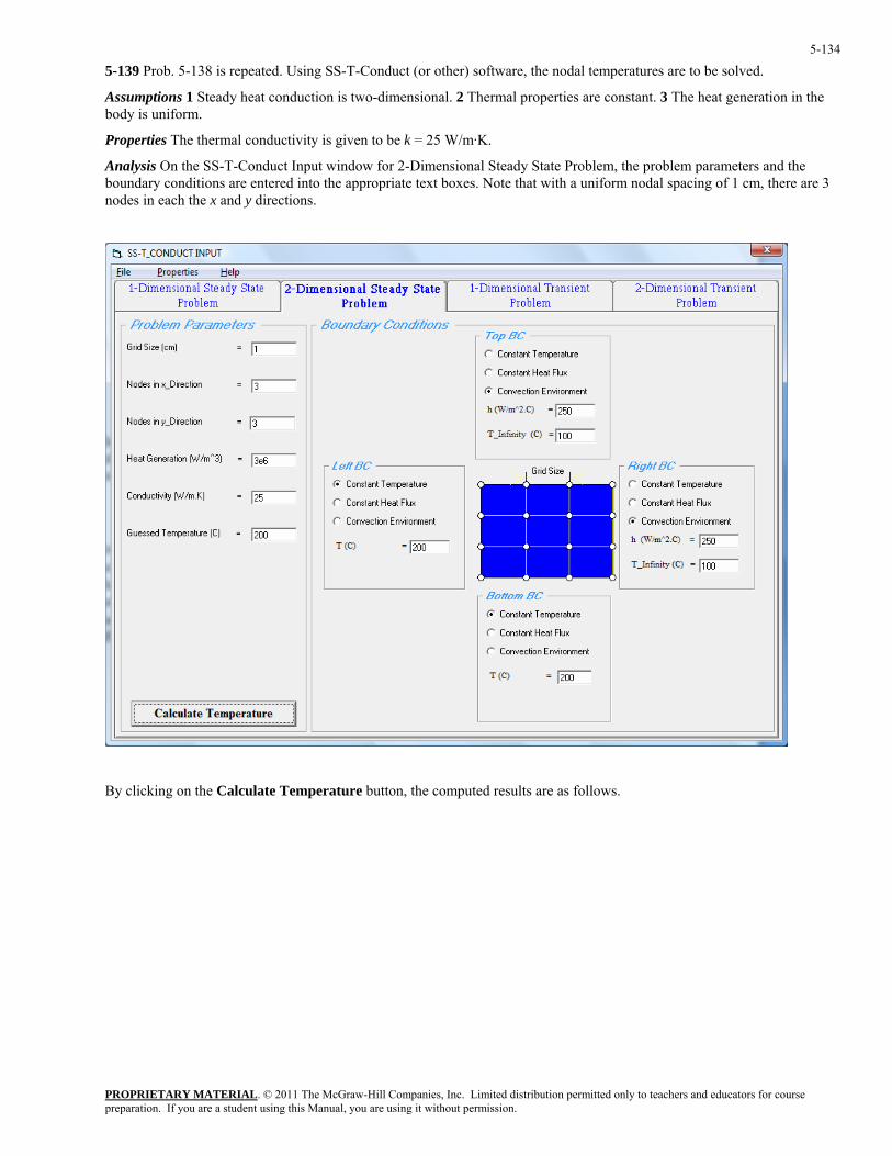
PROPRIETARY MATERIAL. © 2011 The McGraw-Hill Companies, Inc. Limited distribution permitted only to teachers and educators for course preparation. If you are a student using this Manual, you are using it without permission.
5-134
ional. 2 Thermal properties are constant. 3 The heat generation in the ody is uni
is On the SS-T-Conduct Input window for 2-Dimensional Steady State Problem, the problem parameters and the oundary conditions are entered into the appropriate text boxes. Note that with a uniform nodal spacing of 1 cm, there are 3
nodes in each the x and y directions.
5-139 Prob. 5-138 is repeated. Using SS-T-Conduct (or other) software, the nodal temperatures are to be solved.
Assumptions 1 Steady heat conduction is two-dimensb form.
Properties The thermal conductivity is given to be k = 25 W/m·K.
Analysb
B puted results are as follows. y clicking on the Calculate Temperature button, the com
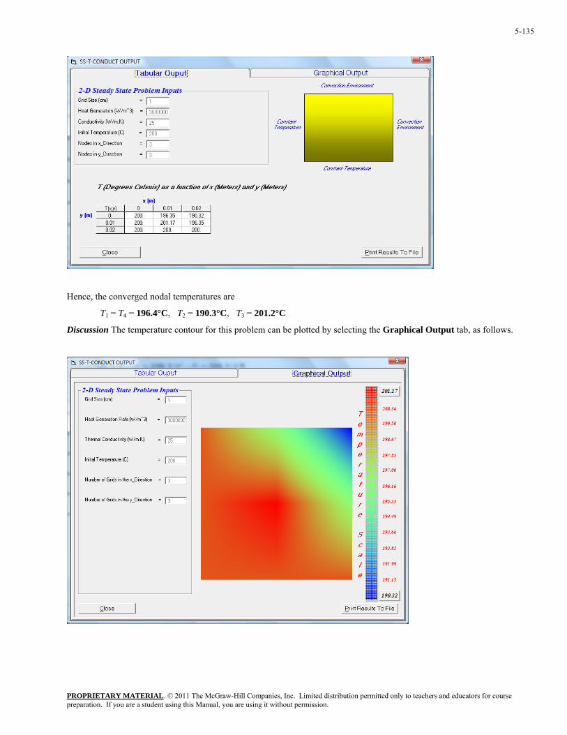
PROPRIETARY MATERIAL. © 2011 The McGraw-Hill Companies, Inc. Limited distribution permitted only to teachers and educators for course preparation. If you are a student using this Manual, you are using it without permission.
5-135
he converged nodal temperatures are
1 4 2 3
Discussion The temperature contour for this problem can be plotted by selecting the Graphical Output tab, as follows.
Hence, t
T = T = 196.4°C, T = 190.3°C, T = 201.2°C
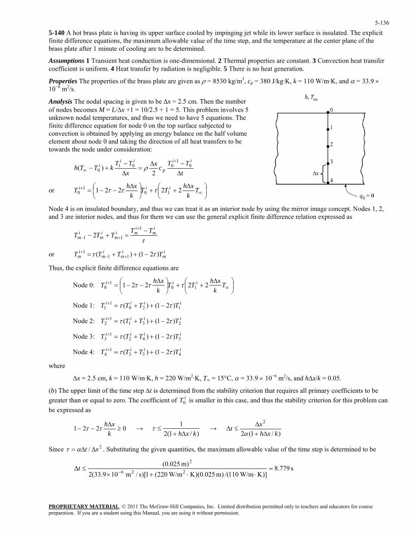
PROPRIETARY MATERIAL. © 2011 The McGraw-Hill Companies, Inc. Limited distribution permitted only to teachers and educators for course preparation. If you are a student using this Manual, you are using it without permission.
5-136
-140 A hot brass plate is having its upper surface cooled by impinging jet while its lower surface is insulated. The explicit finite difference equations, the maximum allowable value of the time step, and the temperature at the center plane of the brass plate after 1 minute of cooling are to be determined.
Assumptions 1 Transient heat conduction is one-dimensional. 2 Thermal properties are constant. 3 Convection heat transfer coefficient is uniform. 4 Heat transfer by radiation is negligible. 5 There is no heat generation.
Properties The properties of the brass plate are given as ρ = 8530 kg/m3, cp = 380 J/kg·K, k = 110 W/m·K, and α = 33.9 × 10⁻⁶ m2/s.
Analysis The nodal spacing is given to be ∆x = 2.5 cm. Then the number of nodes becomes M = L/∆x +1 = 10/2.5 + 1 = 5. This problem involves 5 unknown nodal temperatures, and thus we need to have 5 equations. The finite difference equation for node 0 on the top surface subjected to convection is obtained by applying an energy balance on the half volume element about node 0 and taking the direction of all heat transfers to be towards the node under consideration:
5
tTT
cxxTT
kTThii
p
iii
∆−∆
=∆−
+−+
∞0
1001
0 2)( ρ
⎟⎠⎞
⎜⎝⎛ ∆
++⎟⎠⎞
⎜⎝⎛ ∆
−−= ∞+ T
kxhTT
kxhT iii 22221 10
10 τττ or
Node 4 is on insulated boundary, and thus we can treat it as an interior node by using the mirror image concept. Nand 3 are interior nodes, and thus for them we can use the general explicit finite difference relation expressed as
odes 1, 2,
ii+1
τmmi
mi
mi
mTT
TTT−
=+− +− 11 2
or
Thus, the explicit finite difference equations are
Node 0:
im
im
im
im TTTT )21()( 11
1 ττ −++= +−+
⎟⎠⎞
⎜⎝⎛ ∆
++⎟⎠⎞
⎜⎝⎛ ∆
−−= ∞+ T
kxhTT
kxhT iii 22221 10
10 τττ
Node 1:
Node 2:
Node 3:
Node 4:
where
∆x = 2.5 cm, k = 110 W/m·K, h = 220 W/m2·K, T∞ = 15°C, α = 33.9 × 10⁻⁶ m2/s, and h∆x/k = 0.05.
(b) The upper limit of the time step ∆t is determined from the stability criterion that requires all primary coefficients to be greater than or equal to zero. The coefficient of is smaller in this case, and thus the stability criterion for this problem can be expressed as
iiii TTTT 1201
1 )21()( ττ −++=+
iiii TTTT 2311
2 )21()( ττ −++=+
iiii TTTT 3421
3 )21()( ττ −++=+
iiii TTTT 4331
4 )21()( ττ −++=+
iT0
0221 ≥∆
−−k
xhττ → )/1(2
1kxh∆+
≤τ → )/1(2
2
kxhxt∆+
∆≤∆
α
Since . Substituting the given quantities, the maximum allowable value of the time step is determined to be
2/ xt ∆∆= ατ
s 779.8)]K W/m110/()m 025.0)(K W/m220(1)[s/m 109.33(2
)m 025.0(226
2=
⋅⋅+×≤∆
−t
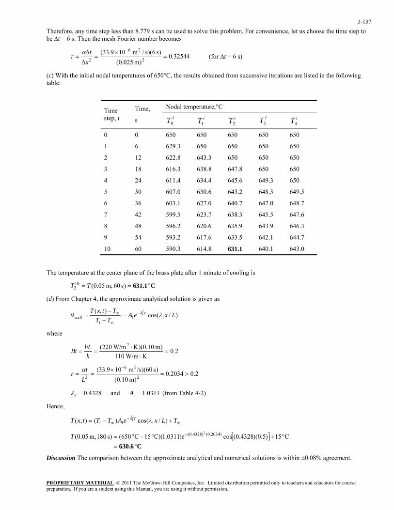
PROPRIETARY MATERIAL. © 2011 The McGraw-Hill Companies, Inc. Limited distribution permitted only to teachers and educators for course preparation. If you are a student using this Manual, you are using it without permission.
5-137
e this problem. For convenience, let us choose the time step to e ∆t = 6 s. Then the mesh Fourier number becomes
Therefore, any time step less than 8.779 s can be used to solvb
32544.0)m 025.0(
)s 6)(s/m 109.33(2
26
2 =×
=∆
∆=
−
xtατ (for ∆t = 6 s)
(c) With the initial nodal temperatures of 650°C, the results obtaine iterationsd from successive are listed in the following table:
Nodal temperature,°C
Time step, i
Time,
s iT0 iT1 iT2 iT3 iT4
0 0 650 650 650 650 650
1 6 629.3 650 650 650 650
650 650 650
647.8 650 650
24 611.4 634.4 645.6 649.3 650
627.0 640.7 647.0 648.7
599.5 623.7 638.3 645.5 647.6
6.2 620.6 635.9 643.9 646.3
617.6 633.5 642.1 644.7
10 60 590.3 614.8 631.1 640.1 643.0
2 12 622.8 643.3
3 18 616.3 638.8
4
5 30 607.0 630.6 643.2 648.3 649.5
6 36 603.1
7 42
8 48 59
9 54 593.2
The temperature at the center plane of the brass plate after 1 minute of cooling is
g en as
C 631.1 °== )s 60 ,m 05.0(2 TT
(d) From Chapter 4, the approximate analytical solution is iv
10
)/cos(),(
11wall21 LxeA
TTTtxT
iλθ τλ−
∞
∞ =−−
=
where
2.0K W/m110
)m 10.0)(K W/m220( 2=
⋅⋅
==k
hLBi
2.02034.0)m 10.0(
)s 60)(/sm 109.33(2
26
2 >=×
==τ −
Ltα
and (from Table 4-2)
Hence,
4328.01 =λ 0311.11 =A
∞−
∞ +−= TLxeATTtxT i )/cos()(),( 1121 λτλ
[ ]C 630.6 °=
°+°−°= − C 15)5.0)(4328.0(cos)0311.1)(C 15C 650()s 180 ,m 05.0( )2034.0()4328.0( 2eT
Discussion The comparison between the approximate analytical and numerical solutions is within ±0.08% agreement.
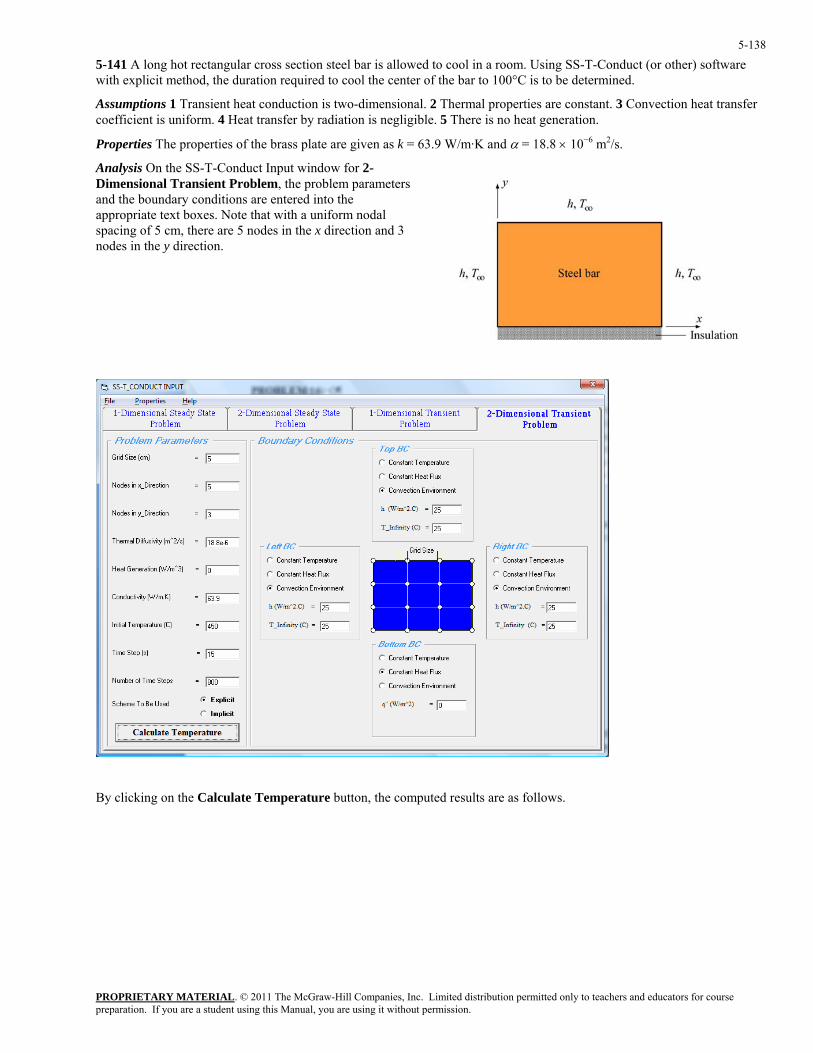
PROPRIETARY MATERIAL. © 2011 The McGraw-Hill Companies, Inc. Limited distribution permitted only to teachers and educators for course preparation. If you are a student using this Manual, you are using it without permission.
5-138
lowed to cool in a room. Using SS-T-Conduct (or other) software center of the bar to 100°C is to be determined.
conduction is two-dimensional. 2 Thermal properties are constant. 3 Convection heat transfer ransfer by radiation is negligible. 5 There is no heat generation.
ate are given as k = 63.9 W/m·K and α = 18.8 × 10⁻⁶ m2/s.
Input window for 2-P m, the problem parameters
entered into the with a uniform nodal
cm, there are 5 nodes in the x direction and 3 y direction.
5-141 A long hot rectangular cross section steel bar is alwith explicit method, the duration required to cool the
Assumptions 1 Transient heatcoefficient is uniform. 4 Heat t
Properties The properties of the brass pl
Analysis On the SS-T-ConductDimensional Transient robleand the boundary conditions areappropriate text boxes. Note thatspacing of 5 nodes in the
By clicking on the Calculate Temperature button, the computed results are as follows.
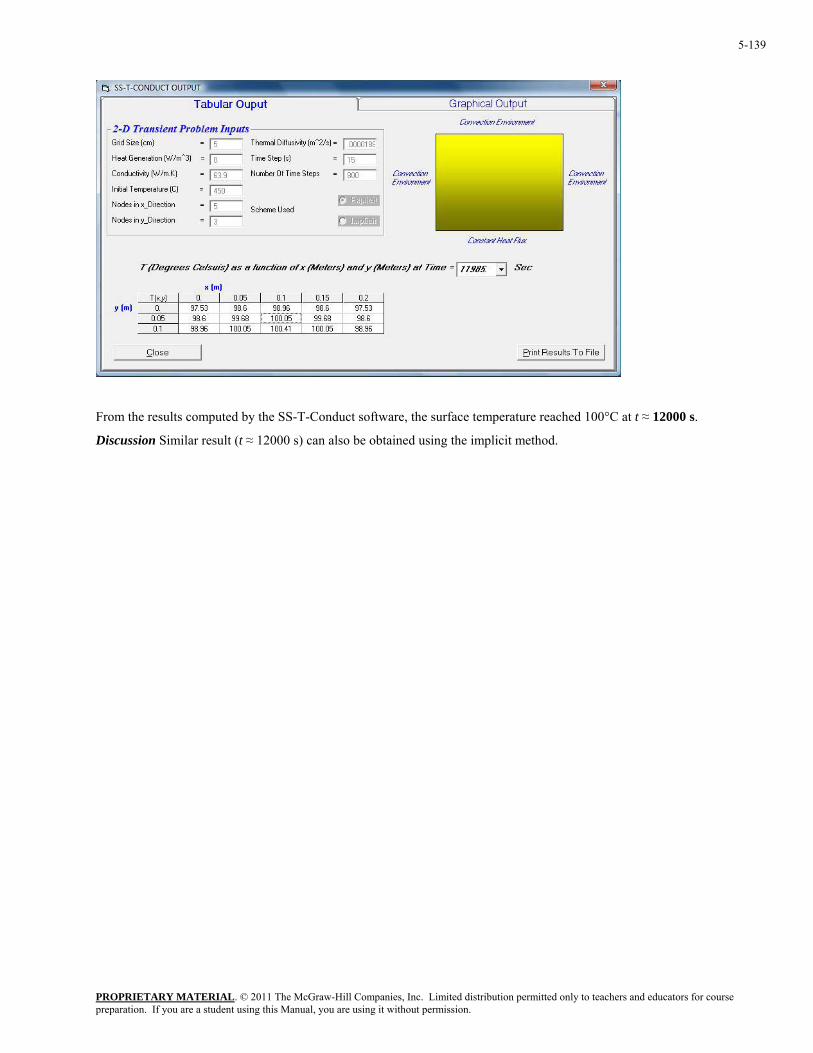
PROPRIETARY MATERIAL. © 2011 The McGraw-Hill Companies, Inc. Limited distribution permitted only to teachers and educators for course preparation. If you are a student using this Manual, you are using it without permission.
5-139
From the results computed by the SS-T-Conduct software, the surface temperature reached 100°C at t ≈ 12000 s.
Discussion Similar result (t ≈ 12000 s) can also be obtained using the implicit method.
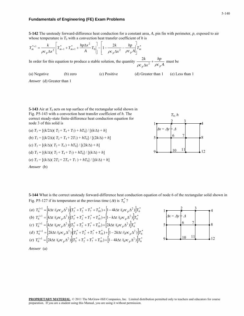
PROPRIETARY MATERIAL. © 2011 The McGraw-Hill Companies, Inc. Limited distribution permitted only to teachers and educators for course preparation. If you are a student using this Manual, you are using it without permission.
5-140
Fundamentals of Engineering (FE) Exam Problems
5-142 The unsteady forward-difference heat conduction for a constant area, A, pin fin with perimeter, p, exposed to air whose temperature is T B0B with a convection heat transfer coefficient of h is
*20
2*
1*
121* 21 m
ppmm
pm T
Achp
xckT
Axhp
TTxc
kT⎥⎥⎦
⎤
⎢⎢⎣
⎡−
∆−−
⎥⎥⎦
⎤
⎢⎢⎣
⎡ ∆++
∆= +−
+
ρρρ
In order for this equation to produce a stable solution, the quantity Ac
hpxc
k
pp ρρ+
∆ 22 must be
(a) Negative (b) zero (c) Positive (d) Greater than 1 (e) Less than 1
Answer (d) Greater than 1
5-143 Air at T B0B acts on top surface of the rectangular solid shown in Fig. P5-143 with a convection heat transfer coefficient of h. The correct steady-state finite-difference heat conduction equation for node 3 of this solid is
(a) T B3B = [(k/2∆)( T B2 B+ T B4 B+ T B7B) + hT B0B] / [(k/∆) + h]
(b) T B3B = [(k/2∆)( T B2 B+ T B4 B+ 2T B7B) + hT B0B] / [(2k/∆) + h]
(c) T B3B = [(k/∆)( T B2 B+ T B4 B) + hT B0B] / [(2k/∆) + h]
(d) T B3B = [(k/∆)( T B2 B+ T B4 B+ T B7B) + hT B0B] / [(k/∆) + h]
(e) T B3B = [(k/∆)( 2T B2 B+ 2T B4 B+ T B7B ) + hT B0B] / [(k/∆) + h]
Answer (b)
5-144 What is the correct unsteady forward-difference heat conduction equation of node 6 of the rectangular solid shown in Fig. P5-127 if its temperature at the previous time (∆t) is *
6T ?
[ ] [ ][ ] [ ][ ] [ ][ ] [ ][ ] [ ] *
62*
10*7
*2
*5
216
*6
2*10
*7
*2
*5
216
*6
2*10
*7
*2
*5
216
*6
2*10
*7
*2
*5
216
*6
2*10
*7
*2
*5
216
)/(41)()/(2 )(
)/(21)()/(2 )(
)/(2)()/( )(
)/(1)()/( )(
)/(41)()/( )(
TctkTTTTctkTe
TctkTTTTctkTd
TctkTTTTctkTc
TctkTTTTctkTb
TctkTTTTctkTa
ppi
ppi
ppi
ppi
ppi
∆∆−++++∆∆=
∆∆−++++∆∆=
∆∆++++∆∆=
∆∆−++++∆∆=
∆∆−++++∆∆=
+
+
+
+
+
ρρ
ρρ
ρρ
ρρ
ρρ
Answer (a)
T B0B, h
• • • • B 1 5 9 B
2 3 B
10 B
6 7 B
11 B
• • • • B
• • • • B
4 8 12 B
∆x = ∆y = ∆B
• • • • B 1 5 9 B
2 3 B
10 B
6 7 B
11 B
• • • • B
• • • • B
4 8 12 B
∆x = ∆y = ∆B
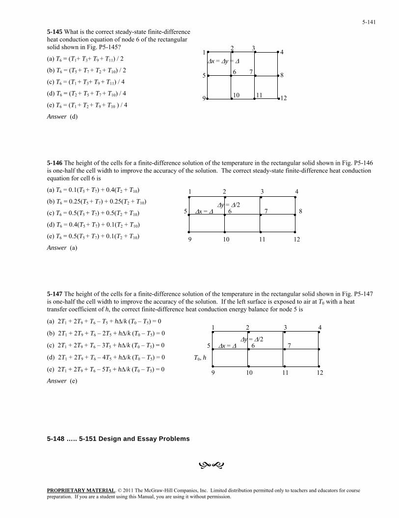
PROPRIETARY MATERIAL. © 2011 The McGraw-Hill Companies, Inc. Limited distribution permitted only to teachers and educators for course preparation. If you are a student using this Manual, you are using it without permission.
5-141
5-145 What is the correct steady-state finite-difference heat conduction equation of node 6 of the rectangular solid shown in Fig. P5-145?
(a) T B6B = (T B1B+ T B3B+ T B9 B+ T B11B) / 2
(b) T B6B = (T B5 B+ T B7 B+ T B2 B+ T B10B) / 2
(c) T B6B = (T B1 B+ T B3B+ T B9 B+ T B11B) / 4
(d) T B6B = (T B2 B+ T B5 B+ T B7 B+ T B10B) / 4
(e) T B6B = (T B1 B+ T B2 B+ T B9 B+ T B10B ) / 4
Answer (d)
5-146 The height of the cells for a finite-difference solution of the temperature in the rectangular solid shown in Fig. P5-146 is one-half the cell width to improve the accuracy of the solution. The correct steady-state finite-difference heat conduction equation for cell 6 is
(a) T B6B = 0.1(T B5 B+ T B7B) + 0.4(T B2B + T B10B)
(b) T B6B = 0.25(T B5 B+ T B7B) + 0.25(T B2B + T B10B)
(c) T B6B = 0.5(T B5 B+ T B7B) + 0.5(T B2B + T B10B)
(d) T B6B = 0.4(T B5 B+ T B7B) + 0.1(T B2B + T B10B)
(e) T B6B = 0.5(T B5 B+ T B7B) + 0.1(T B2B + T B10B)
Answer (a)
5-147 The height of the cells for a finite-difference solution of the temperature in the rectangular solid shown in Fig. P5-147 is one-half the cell width to improve the accuracy of the solution. If the left surface is exposed to air at T B0B with a heat transfer coefficient of h, the correct finite-difference heat conduction energy balance for node 5 is
(a) 2T B1 B + 2T B9B + T B6B – T B5B + h∆/k (T B0B – T B5B) = 0
(b) 2T B1B + 2T B9 B + T B6B – 2T B5B + h∆/k (T B0B – T B5B) = 0
(c) 2T B1 B + 2T B9B + T B6B – 3T B5B + h∆/k (T B0B – T B5B) = 0
(d) 2T B1B + 2T B9 B + T B6B – 4T B5B + h∆/k (T B0B – T B5B) = 0
(e) 2T B1 B + 2T B9B + T B6B – 5T B5B + h∆/k (T B0B – T B5B) = 0
Answer (e)
5-148 ….. 5-151 Design and Essay Problems
1 2 3 4 B
∆y = ∆/2 B
• • • • B
• • • • B
• • • • B
∆x = ∆B 5 6 7 8 B
9 10 11 12 B
1 2 3 4 B
∆y = ∆/2 B
• • • • B
• • • • B
• • • • B
∆x = ∆B 5 6 7
9 10 11 12 B
T B0B, h
• • • • B 1 5 9 B
2 3 B
10 B
6 7 B
11 B
• • • • B
• • • • B
4 8 12 B
∆x = ∆y = ∆B