health inequality between black and white women · health inequality between black and white women...

Institute for Research on Poverty Discussion Paper no. 1251-02

Health Inequality between Black and White Women

Yu-Whuei Hu Department of Economics

National Taiwan University

Barbara Wolfe Departments of Economics and Population Health Sciences

University of Wisconsin–Madison Email: [email protected]

April 2002 An earlier version of this paper was presented at the IHEA 2000 Conference. We thank Betty Evanson for her excellent editing work. We also acknowledge the financial support of the T. Wu Visiting Scholarship of University of Wisconsin–Madison. IRP publications (discussion papers, special reports, and the newsletter Focus) are available on the Internet. The IRP Web site can be accessed at the following address: http://www.ssc.wisc.edu/irp/

Abstract

The black-white inequality in health status in the United States has persisted despite large

increases in life expectancy and improvements in the health status of both races. Our objective is to

examine the inequality in health status between black and white women and to explore the extent to

which such differences are associated with observed dissimilarities in characteristics such as insurance

status, utilization of care, and socioeconomic status. We use data from the 1996 Medical Expenditure

Panel Survey to estimate (reduced-form) health production functions. Based on results of a “Chow-type”

test, separate models are estimated for the black and white samples. To account for the endogeneity of

medical care utilization, we employ a Murphy-Topel two-step econometric method; a Hausman test

rejects the exogeneity hypothesis. According to our medical care utilization estimation, those who are

both poor and uninsured are less likely to use physician services. Controlling for observed factors,

including prior health status, our estimation of the health production function shows that greater use of

medical care and higher educational levels increase the likelihood of being healthy, while lower incomes

and being overweight reduce that likelihood. On the basis of our estimates, we predict that black women’s

likelihood of having excellent health would increase by 3–4 percentage points if they had the same

characteristics, such as number of physician visits, educational level, marital status, weight status, and

income level, as those of their white counterparts.

Health Inequality between Black and White Women

1. INTRODUCTION

Inequality in the health status of blacks and whites in the United States has persisted despite large

increases in life expectancy and improvements in the health status of both races. For example, in 1998 a

6.9-year difference in life expectancy at birth (67.6 vs. 74.5 years) remained between black and white

males, and a 5.2-year difference (74.8 vs. 80 years) existed between black and white females. As of 1997,

the mortality rate of infants born to black mothers was more than double that of those born to white

mothers (14.2 vs. 6 percent). And across different age groups, self-reports of health status differ

systematically. For example, as of 1996, white women were far less likely to report that they were in poor

or fair health than were black women; at ages 18 to 44 the relative proportions were 11 and 19 percent; at

ages 45 to 64 they were 15 and 29 percent; and for women 65 and over, they were 26 and 40 percent,

respectively (Adams, Hendershot, and Marano, 1999.)

In this paper we attempt to address the extent to which such inequality is due to differences in

observed characteristics thought to underlie health outcomes (e.g., medical care utilization, income,

education, etc.) and to what extent it is due to differences in the effects of those characteristics. In other

words, how much of the existing black-white inequality in health would disappear if blacks had the same

observed individual characteristics as whites?1

Unfortunately, the answer to this question is very complicated. Sources of these health

differentials may be associated with low socioeconomic status (e.g., economic barriers to access to

medical services and lack of health insurance due to chronic unemployment), differences in risk-factor

exposures and lifestyle, poorer knowledge of appropriate health practices, more hazardous occupations

1In a recent paper, Deaton and Lubotsky (2001) find that race is likely to be a more powerful factor associated with differences in mortality rates across income/race groups than is income inequality.

2

and environmental exposures, and genetic factors (Behrman et al., 1991; Behrman, Sickles, and Taubman,

1988; Sickles and Taubman, 1986; Kitigawa and Hauser, 1973). Because of the likely interaction of these

factors, we do not attempt to identify the contribution of each separate factor to black-white differentials

in health. Instead, our objective is to explore the inequality in health status between blacks and whites and

to answer the overall question of the extent to which such differences are associated with observed

differences in such characteristics as access to care, education, and socioeconomic status.

We focus on racial inequality in women’s health for two reasons. One, there are well-documented

differences in health between males and females, so we focus on members of only one sex, women, for

ease of analysis. The other is the more limited research in the United States directed at problems specific

to minority women (Kumaryika, Morssink, and Nestle, 2001), suggesting a greater possibility of making

a policy contribution if we can shed some light on possible ways to improve black women’s health status,

thereby reducing the racial inequality in women’s health.

The economics literature on the determinants of women’s health in the context of racial

differences is limited. Two lines of work relate to the issues addressed in this study. The first, work on the

relation of health status and medical care, is based on the theoretic framework of health production first

proposed by Michael Grossman (1972). In this model, the individual is assumed to combine market and

nonmarket inputs according to a household production function to obtain an output of good health

(Grossman, 1972). Health status at a point in time depends on initial health, depreciation of health, and

health investment. Health investment is determined by a weighting of marginal costs and benefits of

health, while health depreciation is related to age and lifestyle.

The second set of contributions concerns the determinants of medical care utilization. Here, we

focus mainly on the role of health insurance. Health insurance plays an important role in access to care.

Literature has shown that more generous coverage will encourage the use of medical care by reducing the

effective price of medical services (Manning et al., 1987; Pauly, 1986; Wolfe and Goddeeris, 1991);

however, issues of endogeneity plague nearly all empirical results. On the other hand, publicly provided

3

health insurance can eliminate the access barrier for those who cannot afford private health insurance

policies. Providing government-financed health programs to all citizens is the way in which many

countries attempt to equalize access to medical care. Of course, equalizing access to care will reduce the

gap in health status between black and white women only to the extent that medical care improves health

status. In this paper, we focus on the tie both between utilization and health and between insurance and

utilization, including the effects of different types of health insurance on medical care utilization. In

particular, we interact income and health insurance to distinguish utilization by the uninsured rich from

that of the uninsured poor.

Although theoretical works assert that medical care is positively associated with health outcomes,

the majority of empirical studies have not confirmed this. One possible reason for the ambiguous effect of

medical care is that medical care utilization may be endogenous in estimating health outcomes. For

example, in many cross-sectional studies, health status and medical care utilization are observed at the

same point in time, so that the frequent utilization of medical care may be the result, rather than the cause,

of poor health. To solve this problem, the use of longitudinal data should be helpful, since the post-

utilization health outcome can be observed. Unfortunately, even in a longitudinal study, the endogeneity

problem may still remain if there are unobserved factors (such as individual tastes) that influence both

medical care utilization and health. Therefore, the estimate of the effect of medical care utilization on

health output may remain inconsistent.

We used panel data from the Medical Expenditure Panel Survey (MEPS) to estimate the effect of

prior utilization of medical services on later (post) health status. We attempt to resolve the issue of the

potential endogeneity of medical care utilization by estimating a two-step maximum likelihood model,

correcting the covariance matrix of the estimates following Murphy and Topel (1985). An alternative to

the two-step procedure is to estimate the first- and second-step models jointly, using an approach such as

full information maximum likelihood (FIML). However, the efficiency and consistency of the estimators

of FIML depend on appropriate specification of the joint distribution. In cases where the proper joint

4

distribution for the econometric models is not known, as is the case here (see Section 2), the two-step

method is more useful, in addition to its advantage in terms of computational simplicity (Murphy and

Topel, 1985).

Many studies of health production functions suffer from a contemporaneous model and/or

inadequate ability to measure health at the beginning of a period, prior to the utilization of medical care

and investment in health-producing activities. In the work presented here, we avoid this problem by using

panel data to measure health at the beginning and at the end of the period. We use a comprehensive set of

measures of prior health in an attempt to fully capture both the need for medical care and chronic

conditions that are likely to continue through the end of the period.

We first describe our conceptual framework and discuss the specification of econometric models

for analyzing the effects of individual characteristics on health. We then present the data and variable

definitions. We discuss our empirical estimates, testing results, and policy simulation, and conclude with

some brief remarks.

2. CONCEPTUAL FRAMEWORK AND ECONOMETRIC MODELS

In the health production framework (Grossman, 1972), an individual is assumed to choose the

optimum level of good health to maximize her utility, subject to her initial health and her monetary and

time constraints. Based on the health effect and direct utility effect of the health inputs, the individual

chooses the optimum combination of health inputs. Through choice of the optimum level of health inputs,

she also determines her health.

A reduced-form version of a health production function is assumed to have the following form:

(1) ,YHCMH 3210* η+α′+α′+α+α=

where *H is the health outcome; M is a measure of medical care utilization; is a vector consisting of

preexisting health conditions;

HC

Y is a vector of health inputs other than medical care and the individual’s

characteristics, which may be variant or invariant through time; and η , which includes unobservable

5

factors and random error. The vector Y includes those factors that influence health outcome directly (e.g.,

lifestyle), those factors that determine health depreciation (e.g., age), those factors that influence the

productivity of gross investment in health (e.g., education), and socioeconomic factors such as income,

gender, and marital status.

As mentioned previously, medical care utilization may be endogenous if some unobservable

factors influence both medical care utilization and health. To test whether medical care is endogenous, we

employ a two-step estimation method. That is, we first estimate the function of medical care utilization,

and then we estimate the health production function, where the observed medical care variable is replaced

with its fitted value.

The individual’s reduced-form function of medical care utilization is assumed to have the

following form:

(2) ,YXHCMlog 3210 ε+β′+β′+β′+β=

where X includes the factors associated with access to care (e.g., the ownership of health insurance) and

opportunity costs regarding time (the presence of children and work status), andε includes unobservable

factors and random error.

If the error terms of equations 1 and 2 share common factors, the result is an inconsistent

estimation of the coefficient of medical care, 1α in equation 1. The two-step method is therefore

employed.

The first step is to estimate medical care utilization. The individual’s utilization of physician

services is our dependent variable. We assume that the number of physician visits, which is a nonnegative

integer variable, follows a negative binomial distribution. The second step is to estimate the health

production function. We do not observe *H , but we do observe an ordered outcome dependent on *H .

6

That is, we select self-assessed health status, say , to represent the individual’s general health status.iH

s

2

The values of represent the ordered rank of her health status (for example, 0=poor, 1=fair, 2=good,

3=very good, and 4=excellent). We replace the observed number of physician visits with its fitted value

obtained from the first-step estimation. Therefore, we estimate the following equation instead of equation

1:

iH

′

(1′) .YHCM̂H 3210* η+α′+α′+α+α=

In Appendix A, we illustrate the maximum likelihood functions for the equations and the

derivation of the correct covariance matrix for α according to Murphy and Topel (1985). We provide a

Hausman test statistic for each two-step model to examine the exogeneity of medical care utilization. If

the exogeniety hypothesis is rejected that is, the test statistic is sufficiently large a two-step model

should be used

In addition, we use a “Chow-type” test (Greene, 2000) to test the hypothesis that all coefficients

of the health production functions for both races are the same. The test statistic is calculated as follows:

],L)LL[(2k PooledWhiteBlack −+×=

where is the test statistic and follows a distribution; and are values of the log-likelihood

functions from the estimation of models for black and white women, respectively; and is the same

measure for the pooled sample of black and white women. If the coefficients are the same, the value of

will be very close to zero. If the “Chow-type” test rejects the above hypothesis, we may conclude that

these individual characteristics influence the health status of black and white women differently. In that

k 2χ BlackL WhiteL

PooledL

k

2Health is clearly a multidimensional outcome. However, in empirical studies, it is difficult to capture multiple aspects and so we use a general measure, self-assessed health rank, which has been shown to be highly correlated with subsequent morbidity and mortality and has proven to be consistent and reliable. (Ware et al., 1978; Smith, 1999).

7

case, racial inequality in health is caused not only by the racial differences in individual characteristics,

but also by racial differences in the effects of those characteristics on health.

3. DATA AND SPECIFICATION

MEPS, cosponsored by the Agency for Health Care Research and Quality and the National

Center for Health Statistics (NCHS), has been collecting nationally representative data on health status

and medical expenditure for the U.S. civilian noninstitutionalized population since 1996. In this study, we

use the household component (HC) of the MEPS (MEPS HC), which includes detailed data on

demographic characteristics, health conditions, health status, use of medical care services, charges and

payments, access to care, satisfaction with care, health insurance coverage, income, and employment.

MEPS HC uses an overlapping panel design in which data are collected through a preliminary

contact followed by a series of five rounds of interviews over a period of 2.5 years. We employ the first

three rounds of the matching samples that contain the individual health information collected in both 1996

and 1997 and the medical care utilization data for the full year 1996. Our initial health measure is based

on data collected approximately 1 year prior to our final measure. The sampling frame for MEPS HC is

drawn from respondents to the National Health Interview Survey (NHIS), conducted by NCHS. NHIS

provides a nationally representative sample of the U.S. civilian noninstitutionalized population, with

oversampling of Hispanics and blacks.

The original sample contains data on 11,768 women. Targeting on nonelderly adult women, we

selected those between 18 and 64 years old (7,681 women). For the ease of analysis, we selected only the

non-Hispanic white and non-Hispanic black women, yielding a total of 5,825 women. We also deleted

those who were pregnant or disabled in 1996 and those with missing values in health status or in the

number of physician visits. In all, our sample for analysis included 4,365 women, 754 of whom were

black.

8

3.1 Variables Included in the Analyses of Medical Care Utilization and Health

Table 1 lists the means and standard deviations of the variables included in the analysis, by race.

Two dependent variables are included in this study, one measuring medical care utilization and the other

measuring current general health status. The total number of physician visits in 1996, which consists of

office-based visits to physicians and hospital outpatient visits to physicians, defines the medical care

utilization variable. Overall, approximately 25 percent of the sample reported no physician visits for the

year. The self-assessed health status collected from the third round of the MEPS survey, in which the

individuals were asked to assess their own overall health status at the beginning of 1997, is used as the

measure of current health status.

Four categories of explanatory variables are included in the models of medical care utilization

and health production: demographic factors, prior health conditions, family income, and geographic

location. The demographic factors, in addition to race (black = 1 if a woman is a non-Hispanic black;

non-Hispanic white is the omitted group), are age (two dummies indicating age groups of 40–54 and 55–

64; 18–39 is the omitted age group), education (years of schooling), and marital status (single = 1 if a

woman is not married or does not cohabit; married is the omitted group). The race variable is included to

test the significance of racial differences with respect to medical care utilization and health status.3 Based

on the theory of demand for health (Grossman, 1972), age determines the individual’s health depreciation

parameter and educational level plays an important role in influencing the productivity of health inputs.

Older individuals are expected to be less healthy and use more medical care owing to their higher

depreciation rate of health stock. Higher educational level is expected to increase the individual’s health

stock; however, its effect on medical care utilization is ambiguous. Many empirical findings have shown

that “married” individuals (including those who cohabit) appear to be healthier than their single

3This variable was omitted in the regression analyses for race-specific subsamples.

9

TABLE 1 Descriptive Statistics of Variables

Black

(n = 754) White

(n = 3,611) Number of Observations Mean Std.Dev. Mean Std.Dev.

Self-Reported Health Statusa Poor 0.03 0.16 0.02 0.14 Fair 0.12 0.33 0.07 0.26 Good 0.31 0.46 0.26 0.44 Very good 0.32 0.47 0.37 0.48 Excellent 0.22 0.42 0.28 0.45

Health Factors Number of conditionsa 1.24 1.52 1.59 1.74 Any work limitation 0.06 0.23 0.07 0.25 Any social limitation 0.03 0.17 0.04 0.20 Number of difficulties performing ADLsa 0.53 1.77 0.44 1.52 Any cancera 0.04 0.20 0.08 0.26 BMI indexa

Obesity 0.25 0.43 0.17 0.38 Severe obesity 0.14 0.35 0.09 0.29

Medical Care Utilization At least one physician visit in year 1996a 0.67 0.47 0.76 0.43 Number of physician visitsa 3.02 4.79 4.23 6.92

Income Categorya Highb 0.23 0.42 0.44 0.50 Middle 0.29 0.45 0.32 0.47 Low or near-poor 0.23 0.42 0.15 0.36 Poor 0.25 0.43 0.09 0.29

Access to Care Health insurancea Public-only health insurance 0.20 0.40 0.08 0.27 Non-HMO private-only insuranceb 0.20 0.43 0.37 0.50 HMO private-only insurance 0.35 0.48 0.40 0.49 No health insurance 0.24 0.43 0.16 0.36

Interaction terms No insurance and middle incomea 0.06 0.24 0.04 0.21 No insurance and near poor or low incomea 0.07 0.26 0.05 0.21 No insurance and poora 0.08 0.27 0.04 0.19

Demographics Age (in years)b 38.77 11.84 40.83 11.95 Agea

Age<40b 0.55 0.50 0.46 0.50 40<=age<=54 0.33 0.47 0.39 0.49 55<=age<=64 0.12 0.32 0.15 0.36

Education (in years)a 12.56 2.30 13.22 2.31 Singlea 0.66 0.48 0.39 0.49

(table continues)

10

TABLE 1, continued

Black

(n = 754) White

(n = 3,611) Number of Observations Mean Std.Dev. Mean Std.Dev. Time Costs

Children under 18 (X)a No children under 18b 0.51 0.50 0.61 0.49 Children aged 0–4 0.15 0.36 0.11 0.32 Children aged 5–13 0.33 0.47 0.28 0.45 Children aged 14–17 0.17 0.37 0.15 0.36

Interaction Terms Single and children aged 0–4a 0.09 0.29 0.03 0.17 Single and children aged 5–13a 0.20 0.40 0.06 0.24 Currently working 0.77 0.42 0.78 0.42 Student 0.06 0.25 0.05 0.23 Have paid sick leave 0.38 0.49 0.36 0.48

Area of Residence Metropolitan statistical areaa 0.85 0.36 0.75 0.44 Northeast 0.22 0.41 0.21 0.40 Midwest 0.20 0.40 0.28 0.45 Southb 0.52 0.50 0.33 0.46 West 0.07 0.26 0.19 0.39

Source: Authors’ calculation based on the Medical Expenditure Panel Survey, 1996. aThe distributions between whites and blacks are statistically different at the 5% level. bVariable is not included in the regression analysis.

11

counterparts.4 Therefore, being single is expected to have a negative association with health, but its

relationship with the demand for medical care is uncertain.

Prior health conditions are included in order to capture health status at the beginning of the

observation period. Individual health conditions were collected in the first round of MEPS, including

number of medical conditions, work limitations, social limitations, cognitive limitations, total number of

difficulties in performing activities of daily living (ADLs), cancer, and obesity measures (obesity = 1 if

body mass index, or BMI, is between 27.3 and 32.3; severe obesity = 1 if BMI>32.3; BMI<27.3 is the

omitted group). Obesity is included because it is considered a risk factor for several diseases, including

breast cancer.5 Other than genetic causes, obesity is associated with aspects of an individual’s lifestyle,

such as insufficient exercise and inappropriate diet or nutrition. Those who are obese are expected to have

poorer health and to use more medical care.

We include three dummy variables to represent family income levels (middle-income, low-

income or near poor, and poor; high-income is the omitted category). Lower family income constrains the

individual’s expenditures, including those for market goods, used to produce health, and is therefore

expected to have a negative effect on both medical care utilization and health status.

3.2 Variables Included Only in the Analysis of Medical Care Utilization

We include two additional categories of variables in the analysis of medical care utilization: time

cost factors and access to care. Time cost factors consist of eight binary variables. The first three variables

indicate whether children of certain ages are present in the family (whether the woman has children

4During the past decade, many researchers have debated the relationship between marriage and mortality rate. Using aggregate or individual-level data, studies provide evidence of lower mortality rates among married couples than among their single counterparts. One potential explanation is based on the protection hypothesis, which assumes that married individuals engage in low-risk activities, share resources, and enjoy caring from each other. The alternative explanation attributes low mortality among married couples to an initial self-selection effect into marriage (Goldman, 1993; Trowbridge, 1994; Waite, 1995; Lillard, 1995; Lillard and Panis, 1996).

5For example, one study found that severe obesity is an explanatory factor for the black-white difference in stage at diagnosis of breast cancer (Jones et al., 1997).

12

whose ages are 0–4, 5–13, or 14–17; having children aged 18 and over is omitted). In addition, we

interact the first two (youngest) groups with the individual’s marital status (single and having children

aged 0–4 or 5–13). Having younger children in the family may reduce an individual’s time available to

devote to health production, while single mothers may have more restricted time for such activities. If the

individual is a mother (or a single mother) of young children, she is expected to use medical services to a

lesser degree.6 Two more variables indicate the individual’s occupational status (whether currently

employed and whether currently a student). If the individual is a worker or a student, she may have higher

opportunity costs of time for health production; she is expected to use less medical care. Finally, we

include a dummy variable indicating whether the individual’s employer provides paid sick leave. If an

employed woman does not have paid sick leave, her time costs for visiting a doctor will be higher, and so

she is expected to use less care.

The last category of variables influencing health are multiple aspects of medical care utilization.

Inequality in access to medical care is often claimed to be a, or the, major factor behind racial differences

in health. Therefore, many public health programs are targeted on equalizing access to care to reduce

racial health inequality. To examine whether lowering the access barriers would reduce racial inequality

in health care and in health, this study considers six variables. Three variables indicate health insurance

status (public health insurance, HMO-type private health insurance, and no health insurance; non-HMO-

type private health insurance is the omitted category). Women who have multiple types of coverage are

included in the public coverage category as all of them have public coverage.7 We expect that in contrast

to those who have non-HMO-type private health insurance, those who have public or HMO-type health

insurance use more physician services, and those who have no health insurance use fewer physician

services. We also expect that those with dual sources of coverage will use more physician services.

Furthermore, we add three variables that interact health insurance status (i.e., no health insurance) with

6Recall that pregnant women are omitted from our sample. 7In an alternative specification, these women are assigned to a separate category of dual coverage.

13

income (middle, low or near-poor, and poor) to distinguish those who choose to be self-insured from

those who cannot afford a health insurance policy. We expect individuals who are poor and have no

health insurance to have reduced access and use fewer physician services.

3.3 Descriptive Data Analysis

The means reported in Table 1 indicate a somewhat better health status for white woman than for

black women. For example, black women are more likely than white women to assess their own health as

poor or fair (15 percent versus 9 percent); are far more likely to be obese or severely obese (39 percent

versus 26 percent); and to report that they have more difficulties in performing activities of daily living

(.53 versus .44). On the other hand, white women are more likely to report the occurrence of specific

health conditions (1.59 versus 1.24), including cancer (0.08 percent versus 0.04 percent), although at least

part of this difference may be tied to white women’s greater access to health care.

In terms of utilization, white women are both more likely to have had at least one physician visit

(76 versus 67 percent) and to have had more visits to a physician than black women (4+ versus 3). The

greater utilization by white women is consistent with the pattern of insurance coverage—white women

are more likely to have coverage; 24 percent of black women report they do not have coverage compared

with 16 percent of white women. If insured, black women are far more likely to have public coverage

than are white women (20 percent versus 8 percent.) In contrast, white women are nearly twice as likely

to have private coverage that is not an HMO (37 percent) than are black women (20 percent).

There are also some notable differences in characteristics of these two groups of women. The

white women are slightly older on average (41 versus 39), have slightly more years of schooling, and are

far less likely to be single (39 versus 66 percent.) The income distribution clearly shows that black

women have lower income than white women—48 percent of black women report their income as poor or

low or near-poor, compared with 24 percent of white women. Black women are more likely to have

children in all three of the age groups and to live in an urban area. Perhaps somewhat surprisingly, the

two groups of women are equally likely to be in the labor force.

14

4. RESULTS

We next present our analysis of the determinants of health status, measured by self-reported

general health status, coded from 0 for poor to 4 for excellent. Given the ordered but categorical nature of

this measure for health, we use an ordered probit maximum likelihood specification. These results are

reported in the last column of Tables 2, 3, and 5. Table 2 presents results for the entire sample of women,

and Tables 3 and 5 present race-specific results. However, as discussed above, including actual utilization

of medical care in the estimate raises problems of endogeneity that is, those people who have health

problems are more likely to use more care. This is the case even though we include several measures of

health at the beginning of the year in which we observe these women; their inclusion reduces but may not

eliminate this problem. Thus we also estimate a two-step model in which the first stage is a prediction of

the number of physician visits and the second stage is an ordered probit similar to that discussed above

but in which the actual utilization is replaced with the predicted utilization derived from the first-stage

estimate. We conduct a statistical test, the Hausman test, to ascertain whether physician utilization is

endogenous in the model.

Based on the test of endogeneity that we conduct, the two-stage model is our preferred

specification; these results are reported in the second and third columns of Tables 2, 3, and 5. The test for

endogeneity (Hausman test) is 67.9 for the combined model; it is significant at the 1 percent level,

indicating that we should rely on the two-step model.

Since the focus of our exploration is race, we turn first to the variable black in Table 2. It has the

expected sign in all three estimates and is significant at the 1 percent level. Being black relative to being

white is associated with fewer physician visits and with poorer health.

We also conduct a test to see whether the same model applies to both races; the test statistic,

based on an F test, clearly indicates that we should rely on the separate estimates, or that the same model

15

TABLE 2 Regression Analysis for Physician Care Utilization and Health Status

(black and white women, 4,365 cases)

Model Number of Physician Visits

Health Status Variable Negative Binomial

Two-Step Ordered Probit

One-Step Ordered Probit

Constant 0.234* (0.12)

2.082*** (0.12)

2.080*** (0.12)

Health Care Utilization Physician visits -0.016***

(0.00) Physician visits (fitted) 0.001

(0.001)

Demographics Race (re: white)

Black -0.238*** (0.05)

-0.177*** (0.05)

-0.189*** (0.05)

Age (re: 18<=age<=39) 40<=age<=54 0.079**

(0.04) -0.121***

(0.04) -0.115*** (0.04)

55<=age<=64 0.188*** (0.05)

-0.070 (0.05)

-0.060 (0.05)

Education (in years) 0.024*** (0.01)

0.076*** (0.01)

0.079*** (0.01)

Marital Status (re: married, coresidence) Single 0.005

(0.04) -0.069*

(0.04) -0.072** (0.04)

Health Factors Number of conditions 0.265***

(0.01) -0.156***

(0.01) -0.132*** (0.01)

Any work limitation 0.432*** (0.08)

-0.533*** (0.08)

-0.499*** (0.08)

Any social limitation 0.276*** (0.09)

-0.232** (0.09)

-0.171* (0.09)

Number of difficulties performing ADLs 0.066*** (0.01)

-0.116*** (0.01)

-0.107*** (0.01)

Any cancer 0.496*** (0.08)

-0.071 (0.06)

-0.034 (0.06)

Obesity or severe obesity 0.093** (0.04)

Obesity -0.150*** (0.05)

-0.142*** (0.05)

Severe obesity -0.297*** (0.06)

-0.294*** (0.06)

(table continues)

16

TABLE 2, continued





Financial Factors Family income level (re: high)

Middle 0.021 (0.04)

-0.056 (0.04)

-0.056 (0.04)

Low or near-poor -0.062 (0.06)

-0.176*** (0.05)

-0.180*** (0.05)

Poor 0.064 (0.07)

-0.285*** (0.06)

-0.286*** (0.06)

Area of Residence (re: not in MSA) Metropolitan statistical area 0.060

(0.04) -0.0003

(0.04) 0.005

(0.04) Geographic location (re: South)

North 0.206*** (0.04)

-0.006 (0.05)

0.008 (0.05)

Midwest 0.026 (0.04)

-0.043 (0.04)

-0.046 (0.04)

West -0.095** (0.05)

0.044 (0.05)

0.034 (0.05)

Time Costs Having children aged 1–4 -0.080

(0.07)

Having children aged 5–13 -0.088* (0.05)

Having children aged 14–17 0.026 (0.05)

Interaction terms: single * X Single and children aged 1–4 0.140

(0.10)

Single and children aged 5–13 -0.056 (0.08)

Currently working -0.030 (0.04)

Student -0.298*** (0.09)

Employer-provided paid sick leave 0.066 (0.04)

(table continues)

17

TABLE 2, continued





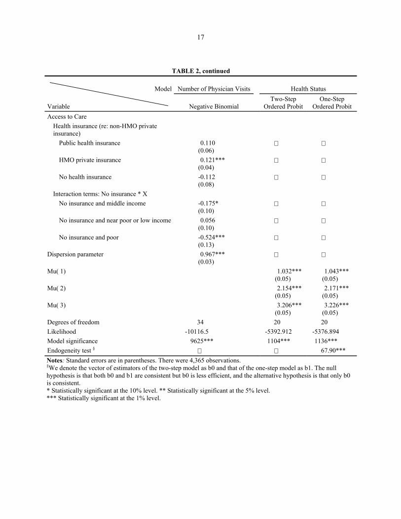
Access to Care Health insurance (re: non-HMO private insurance)

Public health insurance 0.110 (0.06)

HMO private insurance 0.121*** (0.04)

No health insurance -0.112 (0.08)

Interaction terms: No insurance * X No insurance and middle income -0.175*

(0.10)

No insurance and near poor or low income 0.056 (0.10)

No insurance and poor -0.524*** (0.13)

Dispersion parameter 0.967*** (0.03)

Mu( 1) 1.032*** (0.05)

1.043*** (0.05)

Mu( 2) 2.154*** (0.05)

2.171*** (0.05)

Mu( 3) 3.206*** (0.05)

3.226*** (0.05)

Degrees of freedom 34 20 20 Likelihood -10116.5 -5392.912 -5376.894 Model significance 9625*** 1104*** 1136*** Endogeneity test § 67.90*** Notes: Standard errors are in parentheses. There were 4,365 observations. §We denote the vector of estimators of the two-step model as b0 and that of the one-step model as b1. The null hypothesis is that both b0 and b1 are consistent but b0 is less efficient, and the alternative hypothesis is that only b0 is consistent. * Statistically significant at the 10% level. ** Statistically significant at the 5% level. *** Statistically significant at the 1% level.

18

does not apply to members of both races.8 The test statistics for both the utilization and health status

equations are significant at the 1 percent level, which means that their overall effects differ between black

and white women. Therefore, we focus primarily on our estimates for black and white samples separately,

and we discuss the results for black women in Table 3 and white women in Table 5.

4.1 Determinants of Health and Medical Care Use among Black Women

Insurance clearly is associated with medical care use among black women (Table 3). Women

with HMO private insurance use more care; women with no insurance and whose incomes are in the

middle-income category or less receive less care. Those with public insurance seem to use more care, but

the coefficient is not statistically significant. Black women who have more adverse health conditions and

those who have cancer use more care than other women. Few other variables are statistically significant,

with the exception of the negative associations between the use of care by women who are students and

women who have children aged 5–13.

Turning to the determinants of health status among black women, we find that women who use

more care (our fitted value from stage one described above) have better health. Women who have poorer

health at the beginning of the period in terms of more health conditions, a work limitation, difficulties

performing ADL’s, or cancer report poorer health at the end of the period than do other women. Women

who are severely obese also report poorer health than women who are thinner. Women with more years of

schooling report better health. The only relationship that might seem somewhat surprising is the negative

association between being aged 40–54 and health status. This is not surprising among the younger

omitted age group, but it is surprising among the older group, those aged 55–64 (although the coefficient

on the 55–64 dummy variable is negative, is smaller in magnitude than the 40–54 coefficient, and is not

8For the analysis of medical care utilization, the test statistic is .

For the analysis of health status, it is .

82)]10126()8565()1520[(21k =−−−+−×=

54)]5400()4389()984[(22k =−−−+−×=

19


(black women, 754 cases)

Model Number of Physician Visits Health Status

Variable (Negative Binomial) (Two-Step Ordered Probit) Constant 0.059

(0.42) 1.820***

(0.30) Health Care Utilization

Physician visits (fitted)

0.006 (0.01)

Demographics Age (re: 18<=age<=39)

40<=age<=54 -0.048 (0.12)

-0.301*** (0.10)

55<=age<=64 0.151 (0.18)

-0.105 (0.13)

Education (in years) 0.032 (0.02)

0.074*** (0.02)

Marital status (re: married, coresidence) Single 0.053

(0.15) -0.074 (0.09)


(0.03) -0.143*** (0.03)

Any work limitation 0.400 (0.29)

-0.490*** (0.18)

Any social limitation 0.502 (0.36)

-0.291 (0.29)

Number of difficulties performing ADLs 0.065 (0.04)

-0.092*** (0.03)

Any cancer 0.601** (0.27)

-0.410** (0.18)

Obesity or severe obesity 0.033 (0.10)

Obesity

-0.070 (0.10)

Severe obesity

-0.329** (0.13)


Middle 0.142 (0.15)

0.163 (0.12)


-0.114 (0.13)

Poor 0.161 (0.21)

-0.114 (0.13)

Area of Residence (re: not in MSA) Metropolitan statistical area -0.204

(0.15) 0.004

(0.11)

(table continues)

20

TABLE 3, continued


Variable (Negative Binomial) (Two-Step Ordered Probit) Geographic location (re: South)

North 0.216 (0.14)

0.008 (0.10)

Midwest 0.169 (0.13)

-0.044 (0.12)

West 0.202 (0.19)

0.107 (0.17)

Time Costs Children aged 0–4 -0.108

(0.29)

Children aged 5–13 -0.483** (0.22)

Children aged 14–17 -0.114 (0.13)

Interaction terms: single * X Single and children aged 0–4 -0.151

(0.33)

Single and children aged 5–13 0.257 (0.26)


Student -0.798*** (0.25)

Employer provide paid sick leave 0.028 (0.13)



HMO private insurance 0.202** (0.13)

No health insurance 0.696*** (0.24)

Interaction terms: No insurance * X No insurance and Middle income -1.316***

(0.35)

No insurance and low or near-poor income -0.911*** (0.33)

No insurance and poor -1.437*** (0.32)

(table continues)

21

TABLE 3, continued


Variable (Negative Binomial) (Two-Step Ordered Probit) Dispersion Parameter 0.997***

(0.09)

Mu( 1) 1.101*** (0.11)

Mu( 2) 2.179*** (0.11)

Mu( 3) 3.134*** (0.12)

Likelihood -1522 -986 Degrees of freedom 33 19 Model significance (chi-square statistic) 1109*** 165*** Notes: Standard errors are in parentheses. Dispersion parameter measures the size of dispersion. If the parameter is significant, the hypothesis that the mean equals the variance is rejected and the negative binomial model is more appropriate for the data. These Mu(I)’s are the estimates of the thresholds of health ranks from the Ith rank to the (I+1)th rank, I=1,2,3. * Statistically significant at the 10% level. ** Statistically significant at the 5% level. *** Statistically significant at the 1% level.

22

significant). None of the other included factors, such as income and area of residence, are significantly

related to health. Thus, once prior health status is controlled for, the factors that might improve health are

education, medical care, and weight (obesity). How much difference might these make? In Table 4 we

calculate the marginal effects of the factors included in the regressions both on physician visits and on

health status. Health status is presented as the increased or decreased probability of having poor, fair,

good, very good, and excellent health. Right-hand-side variables are held at their means except for

variables for which marginal effects are being calculated.

The marginal effects suggest that having one more physician visit is associated with a of 0.02

percentage point reduction in being in poor health or a 0.15 percentage point increase in being in excellent

health. Going from age 39 or younger to age 40–54 is associated with a 0.92 percentage point increase in

the probability of being in poor health and a reduction of 8.18 percentage points in being in excellent

health. Having 1 more year of schooling is associated with being 0.23 of a percentage point less likely to

be in poor health and 2.01 percentage points more likely to be in excellent health. Those women who are

severely obese have a 5.6 percentage point greater probability of being in fair health and about a 9

percentage point lower probability of being in excellent health than do thinner women. Prior health status

is highly associated with subsequent health, so black women with one additional health condition are

nearly 4 percentage points less likely to have excellent health than other black women. Black women with

any work limitation are more than 13 percentage points less likely to be in excellent health, and those who

had cancer at the beginning of the period are 11 percentage points less likely to be in excellent health. A

woman with one more limitation in ADLs than an otherwise similar woman has a 2.5 percentage point

lower probability of being in excellent health.

4.2 Determinants of Health and Medical Care Use among White Women

As with black women, insurance coverage is a determinant of health care utilization by white

women, although the pattern differs somewhat (Table 5). All white women without insurance use less

care, especially among those who are poor. Women with HMO-based private insurance use more care (as

23

TABLE 4 Marginal Effects of Characteristics on Number of Physician Visits and Likelihood of Various Health Statuses

(black women, 754 cases)

Likelihood of Health Status Being

Variable

Number Physician

Visits Poor Fair Good Very Good Excellent

Constant 0.128 -0.0556 -0.3123 -0.3554 0.2296 0.4940 Physician visits -0.0002 -0.001 -0.0011 0.0007 0.0015 40<=age<=54 -0.105 0.0092 0.0517 0.0589 -0.0380 -0.0818 55<=age<=64 0.331 0.0032 0.018 0.0205 -0.0132 -0.0285 Education 0.071 -0.0023 -0.0127 -0.0145 0.0093 0.0201 Single 0.117 0.0023 0.0127 0.0145 -0.0094 -0.0201 Number of conditions 0.732 0.0044 0.0245 0.0279 -0.0180 -0.0388 Any work limitation 0.876 0.0149 0.084 0.0956 -0.0618 -0.1329 Any social limitation 1.101 0.0089 0.0499 0.0569 -0.0367 -0.0790 Number of difficulties performing ADLs 0.143 0.0028 0.0157 0.0179 -0.0116 -0.0249 Any cancer 1.317 0.0125 0.0703 0.08 -0.0517 -0.1113 Obesity or severe obesity 0.073 Obesity 0.0021 0.0119 0.0136 -0.0088 -0.0189 Severe obesity 0.01 0.0564 0.0642 -0.0415 -0.0892 Middle income 0.311 -0.005 -0.0279 -0.0318 0.0205 0.0442 Near poor or low income -0.493 0.0035 0.0196 0.0223 -0.0144 -0.0310 Poor income 0.353 0.0035 0.0195 0.0222 -0.0143 -0.0309 Metropolitan statistical area -0.448 -0.0001 -0.0007 -0.0008 0.0005 0.0010 North 0.474 -0.0002 -0.0014 -0.0016 0.0010 0.0022 Midwest 0.370 0.0013 0.0075 0.0085 -0.0055 -0.0119 West 0.444 -0.0033 -0.0183 -0.0209 0.0135 0.0290 Children aged 0–4 -0.236 Children aged 5–13 -1.059 Children aged 14–17 -0.251 Single and children aged 0–4 -0.330 Single and children aged 5–13 0.564 Currently working 0.007 Student -1.749 Employer-provided paid sick leave 0.061 Public health insurance 0.326 HMO private insurance 0.442 No health insurance 1.526 No insurance and middle income -2.885 No insurance and low or near-poor income -1.996 No insurance and poor -3.150 Note: Bold figures indicate statistical significance at 1%~10% level.

24


(white women, 3,611 cases)

Model Number of outpatient Visits Health Status Variable Negative Binomial Two-Step Ordered Probit Constant 0.202

(0.13) 2.093***

(0.13) Health Care Utilization

Physician visits (fitted) 0.002* (0.001)

Demographics Age (re: 18<=age<=39)

40<=age<=54 0.090** (0.04)

-0.083** (0.04)

55<=age<=64 0.194*** (0.06)

-0.070 (0.06)

Education (in years) 0.028*** (0.01)

0.078*** (0.01)

Marital status (re: married, coresidence) Single -0.035

(0.05) -0.066* (0.04)


(0.01) -0.165*** (0.01)

Any work limitation 0.439*** (0.09)

-0.539*** (0.09)

Any social limitation 0.266*** (0.09)

-0.241** (0.10)

Number of difficulties performing ADLs 0.061*** (0.02)

-0.128*** (0.02)

Any cancer 0.490*** (0.08)

0.022 (0.07)

Obesity or severe obesity 0.109*** (0.04)

Obesity -0.179*** (0.05)

Severe obesity -0.297*** (0.07)


Middle 0.009 (0.05)

-0.088** (0.04)


-0.168 (0.06)

Poor 0.036 (0.09)

-0.334*** (0.07)

Area of Residence (re: not in MSA) Metropolitan statistical area 0.078*

(0.05) 0.003

(0.04) (table continues)

25

TABLE 5, continued

Model Number of outpatient Visits Health Status Variable Negative Binomial Two-Step Ordered Probit Geographic Location (re: South)

North 0.189*** (0.05)

-0.009 (0.05)

Midwest -0.001 (0.05)

-0.047 (0.05)

West -0.128** (0.05)

0.033 (0.05)

Time Costs Children aged 0–4 -0.076

(0.07)

Children aged 5–13 -0.060 (0.05)

Children aged 14–17 0.045 (0.05)

Interaction terms: single * X Single and children aged 0–4 0.277**

(0.12)

Single and children aged 5–13 -0.072 (0.09)


Student -0.190 (0.10)

Employer-provided paid sick leave 0.079* (0.04)



HMO private insurance 0.109*** (0.04)

No health insurance -0.324*** (0.10)

Interaction terms: no insurance * X No insurance and middle income 0.106

(0.13)

No insurance and low or near-poor income 0.312 (0.13)

No insurance and poor -0.275* (0.16)

(table continues)

26

TABLE 5, continued

Model Number of outpatient Visits Health Status Variable Negative Binomial Two-Step Ordered Probit Dispersion Parameter 0.946***

(0.03)

Mu( 1) 1.013*** (0.06)

Mu( 2) 2.153*** (0.06)

Mu( 3) 3.231*** (0.06)

Likelihood -8565 -4376 Degrees of freedom 33 19 Model significance (chi-square statistic) 8355*** 964***

Notes: Standard errors are in parentheses. Dispersion parameter measures the size of dispersion. If the parameter is significant, the hypothesis that the mean equals the variance is rejected and the negative binomial model is more appropriate for the data. These Mu(I)’s are the estimates of the thresholds of health ranks from the Ith rank to the (I+1)th rank, I=1,2,3. * Statistically significant at the 10% level. ** Statistically significant at the 5% level. *** Statistically significant at the 1% level.

27

is the case with black women), and those with public insurance register a positive coefficient, but it is not

significant. Women with poorer health, such as more medical conditions, any work limitation, any social

limitation, any cancer, or difficulties with ADLs, all use more care. Women who are obese use more

medical care. In contrast to black women, other factors among white women are also significantly related

to medical care use. Older women use more care, as do those who live in an urban area, those who are

single, and those who have a child under age 5. There is also some indication that women whose

employers provide paid sick leave are somewhat more likely to use more care.

Turning to the health status equation for white women, we again find that having poor health at

the beginning of the period as measured by number of health conditions, a work or social limitation, or

more difficulties performing ADLs are all associated with a higher probability of reporting poorer

health at the end of the period. Again, being obese is associated with poorer health, although among white

women being obese and being severely obese are associated with poorer health, while among black

women only those with severe obesity had a significantly greater probability of reporting poorer health

than thinner women. White women who use more medical care (measured by the fitted value) are

somewhat more likely to have better health, but the coefficient is small and is significant only at the 10

percent level. White women whose family income is not high are less likely to have excellent health,

especially women who are poor or those of middle income. Single women also appear to be less likely to

be healthy. Women with more education appear to be more likely to have better health. As with black

women, white women aged 40–54 appear more likely to have poorer health than those who are younger,

but also than those who are somewhat older.

How much difference might these factors make? In Table 6 we calculate the marginal effects of

the included variables both on physician visits and on health status among white women. As in Table 4,

health status is presented as the increased or decreased probability of having poor, fair, good, very good,

and excellent health. Right-hand-side variables are held at their means except for the variables for which

marginal effects are calculated.

28

TABLE 6 Marginal Effects on Number of Physician Visits and Likelihood of Various Health Statuses

(based on sample mean, white women, 3,611 cases)

Likelihood of Health Status Being

Variable

Number Physician

Visits Poor Fair Good Very Good Excellent

Constant 0.685 -0.0328 -0.2257 -0.5150 0.1304 0.6489 Physician visits 0.00003 -0.0002 -0.0005 0.0001 0.0007 40<=age<=54 0.305 0.0013 0.0089 0.0204 -0.0052 -0.0257 55<=age<=64 0.659 0.0011 0.0076 0.0173 -0.0044 -0.0218 Education 0.095 -0.0012 -0.0084 -0.0192 0.0049 0.0241 Single -0.118 0.0010 0.0072 0.0163 -0.0041 -0.0206 Number of conditions 0.874 0.0026 0.0178 0.0406 -0.0103 -0.0512 Any work limitation 1.491 0.0085 0.0582 0.1327 -0.0336 -0.1672 Any social limitation 0.905 0.0038 0.0260 0.0593 -0.0150 -0.0748 Number of difficulties performing ADLs 0.206 0.0020 0.0138 0.0316 -0.0080 -0.0398 Any cancer 1.664 0.0004 0.0024 0.0055 -0.0014 -0.0070 Obesity or severe obesity 0.370 Obesity 0.0028 0.0193 0.0441 -0.0112 -0.0555 Severe obesity 0.0047 0.0320 0.0730 -0.0185 -0.0920 Middle income 0.032 0.0014 0.0095 0.0217 -0.0055 -0.0274 Low or near-poor income -0.093 0.0026 0.0181 0.0414 -0.0105 -0.0521 Poor income 0.123 0.0052 0.0360 0.0822 -0.0208 -0.1035 Metropolitan statistical area 0.266 0.0000 0.0003 0.0008 -0.0002 -0.0010 North 0.641 0.0001 0.0010 0.0023 -0.0006 -0.0029 Midwest -0.002 0.0007 0.0051 0.0117 -0.0030 -0.0147 West -0.433 -0.0005 -0.0036 -0.0082 0.0021 0.0103 Children aged 0–4 -0.259 Children aged 5–13 -0.205 Children of aged 14–17 0.153 Single and children aged 0–4 0.941 Single and children aged 5–13 -0.244 Currently working -0.134 Student -0.646 Employer-provided paid sick leave 0.268 Public health insurance 0.344 HMO private insurance 0.369 No health insurance -1.101 No insurance and middle income 0.358 No insurance and near poor or low income 1.060 No insurance and poor -0.934 Note: Bold figures indicate statistical significance at 1%~10% level

29

The marginal effects suggest that having one more physician visit is associated with a 0.07

percentage point increase in being in excellent health. Women aged 40–54, relative to those aged 39 or

younger, appear to have a 0.09 percentage point greater chance of having fair health and a 2.6 percentage

point reduction in the likelihood of being in excellent health. Women with more education again seem

more likely to be healthy. At the margin, women with an additional year of schooling have a 2.4

percentage point greater probability of being in excellent health. Women who are single have a 2.1

percentage point lower probability of being in excellent health than do married women. Having a health

condition at the beginning of the period has a large marginal association with health; at the margin,

women with one more prior health condition are 5.1 percentage points less likely to report excellent

health and nearly 2 percentage points more likely to report poor or fair health. Women with a work or

social limitation are far less likely than other women to report excellent health (the marginal effect is !17

percentage points for presence of a work limitation and !7.5 percentage points for a social limitation).

Women who report that they are severely obese have a 9 percentage point lower probability of being in

excellent health (and nearly 4 percentage points lower than women who report they are obese). Women

whose family income places them below the poverty line have a marginal probability of being in excellent

health that is more than 10 percentage points below that of other women.

As a test of robustness of our model, and because work itself may be endogenous and influence

health and utilization, we also conduct this analysis after dividing the women into groups by labor force

participation no participation, full-time work, and part-time work. We do this for white women

separately and for the entire group; there are too few black women to successfully conduct the analysis on

some of these subgroups. The descriptive statistics show the expected pattern, namely that women who do

not work tend to be older, less healthy, and less likely to have private coverage. The racial differences

noted above remain in the descriptive statistics.9 The analysis of the determinants of utilization and health

9These tables are available from the authors.

30

status by labor force participation subgroups tends to show the same pattern as that reported above for the

entire group of white women. To the extent that there are differences, they seem to be concentrated in the

utilization estimates. White women who work full-time seem more responsive to type of coverage than

other white women and to receive more care if they have a health condition than do other white women.

The results for determinants of health status are generally consistent with those discussed above for all

white women.

4.3 Disentangling Reasons for the Poorer Health of Black Women

Using the coefficients from the model that we estimated over our sample of black women and the

characteristics of the white women in our sample, we now attempt to disentangle the reasons for which

black women’s health is worse than that of white women. In particular, we would like to know the extent

to which black women’s care utilization and health status would change if their observed characteristics

were identical to those among our sample of white women. To do so, we multiply the difference in the

black and white means of selected characteristics by the marginal effects of these variables from our two-

stage model. The results of the simulation for utilization and health status are reported in Tables 7 and 8.

We report on the expected effect of a number of individual factors, and at the bottom of each table we

report on the overall change in utilization or health status that our model predicts if black women had the

same observed characteristics, in terms of education, marital status, income, and insurance status, as the

white women in our sample. In terms of utilization (Table 7), we expect that on average, black women

would increase their number of provider visits by .19, or by 6.5 percent, were they to have the same

characteristics as white women. This is still far below the mean number of visits by white women (4.23

visits per year).

In terms of health status (Table 8), we note some larger changes. If black women had white

women’s observed characteristics, including their predicted higher use of medical care, we expect that

black women on average would have a 13 percent lower probability of reporting poor health, a 19 percent

lower probability of reporting fair health, and an 8 percent lower probability of reporting good health. In

31

TABLE 7

Changes in Marginal and Total Effects of Selected Individual Characteristics on Mean Number of Physician Visits, if Blacks Had Whites’ Characteristics

Characteristics

Changes in Marginal Effect on Mean Number of Physician Visits

Mean Difference (White-Black)

Education 0.04704 0.66060 Single -0.03160 -0.27073 Middle income 0.00998 0.03206 Low or near-poor income 0.03945 -0.08006 Poor income -0.05394 -0.15286 Public health insurance 0.013931 0.04267 HMO private insurance -0.03826 -0.08652 No health insurance -0.02994 -0.01963 No insurance and middle income 0.07525 -0.02609 No insurance and near poor or low income 0.087543 -0.04385 No insurance and poor 0.075437 -0.02395 Total effects on mean number of physician visits 0.19489 Actual mean number of physician visits by black women 3.02 Percentage change 6.45

32

TABLE 8

Changes in Marginal and Total Effects of Selected Individual’s Characteristics on Likelihood of Having Different Health Ranks, if Blacks Had Whites’ Characteristics

Health Rank

Characteristics Poor Fair Good Very Good Excellent

Mean Difference

(White-Black)

Number of physician visits -0.000242 -0.001208 -0.001329 0.000846 0.001872 1.20836 Education -0.001519 -0.00839 -0.009579 0.006012 0.013282 0.66060 Single -0.000623 -0.003438 -0.003926 0.002464 0.005447 -0.27073 Obesity -0.000164 -0.000928 -0.00106 0.000671 0.001473 -0.07798 Poor income -0.000535 -0.002981 -0.003394 0.002140 0.004719 -0.15286

Total effects on likelihood of having different health status -0.00403 -0.02225 -0.02532 0.015942 0.035179 Actual proportion 0.03 0.12 0.31 0.32 0.22 Percentage change -13% -19% -8% 5% 16%

33

contrast, they would have a 5 percent greater probability of reporting very good health and a 16 percent

higher probability of reporting excellent health. Even with these changes, black women would still be

reporting poorer health than white women, but the differences would be substantially decreased. For

example, black women are actually 1.7 times more likely than white women to report fair health, but if

their observed characteristics were like those of white women, this ratio would be reduced to 1.4. And if

their observed characteristics were like those of white women, the ratio of the probability that they would

be in excellent health would go from 0.8 to 0.9.

The factors most important in accounting for such shifts to better health are, in order of

importance, a higher level of education, a decline in the proportion single, a decrease in the proportion

poor, and a decline in the proportion severely obese.

4.4 Potential Impact of Changes in Health Insurance System on Utilization and Health for Black and White Women

Among all the policy instruments for improving health, reducing barriers to care is the most

recognized and widely used approach in many countries. This may take the form of universal coverage or

subsidies to encourage the private sector to provide coverage. Here, we ask to what extent a change in

health insurance coverage would change utilization and health. Using the coefficients from the model

estimated over our samples of black and white women, we design two policy simulations to gauge the

overall effects of changing the health insurance system on utilization and health. In the first, we assume

that all women have private HMO health insurance, and in the other we assume that all those who are

uninsured obtain public coverage. We present the results for black and white women in Tables 9 and 10,

respectively. The procedure used for these simulations is given in Appendix B.

If all women were covered only by private HMO insurance (including those with other forms of

coverage and those without coverage), we predict a 16 percent increase in physician visits by black

34

TABLE 9

Potential Impacts of Changes in Health Insurance System on Utilization and Health Status of Black Women

All Covered by Private HMO Insurance (N=754)

All Those without Insurance Get Public Coverage (N=183)

New Health Insurance System New Prediction % Change New Prediction % Change Mean number of physician visits 4.79 16 4.87 18

Health Status % % Change % % Change

Poor or fair 4.64 -20 5.46 -19

35

TABLE 10

Potential Impacts of Changes in Health Insurance System on Utilization and Health Status of White Women

All Covered by Private HMO Insurance (N=3611)

All Those without Insurance Get Public Coverage (N=564)

New Health Insurance System New Prediction % Change New Prediction % Change Mean number of physician visits 5.70 11 7.41 45

Health Status % % Change % % Change

Poor or fair 2.99 -2 3.37 -85

36

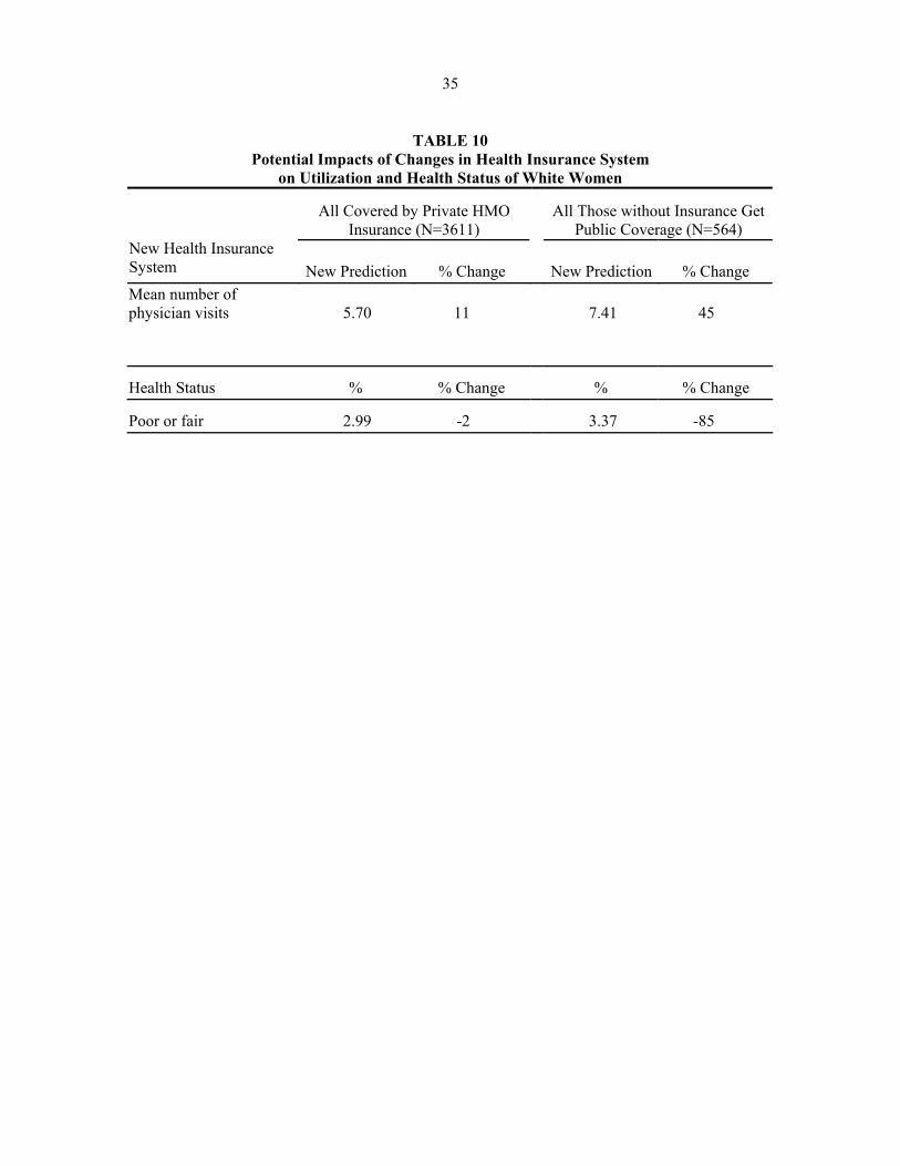
women and an 11 percent increase by white women. The expected change in terms of health10 is also

substantial, reducing the proportion in poor or fair health among black women by 20 percent, versus only

2 percent for white women.11

Last, we turn to those who have no health insurance (183 black women and 564 white women).

We simulate the potential changes in their medical care utilization if all were to obtain public coverage.

For both races we find that the effect of providing public health coverage to those who are uninsured is

substantial an expected 18 percent increase in the mean number of physician visits for black women and

a 45 percent increase for white women. This supports the notion that providing health insurance to the

uninsured can lower the barrier to care and increase utilization. In terms of health status, the uninsured

will be much less likely to report that they are in poor health; more specifically, we simulate a 19 percent

reduction in the proportion who report poor or fair health among black women and an 85 percent

reduction for white women. It is interesting to note that the policy change may benefit white women’s

health more than black women’s health.

5. CONCLUSION

In this paper we have explored the determinants of black and white women’s health status and

health care utilization. Our purpose has been to learn whether the differences are largely due to

differences in observed characteristics ranging from unchangeable factors such as race and age to partially

changeable factors such as education to changeable factors such as insurance coverage. Or, to what extent

do the sizable differences in health status reflect differential relationships between observed

characteristics and these outcomes? We find, not surprisingly, that both observed factors and differential

relationships play a role.

10We choose the health rank that has the largest predicted likelihood as the individual’s health status. 11Among black women this is entirely a reduction of the proportion in poor health. Among white women

there is a 4 percent reduction in the proportion in poor health, which is offset by a shift of half of these women to fair health.

37

In terms of utilization, we find little change among black women were they to have white

women’s observed characteristics. However, we find that black women’s health status is expected to

improve considerably. In particular we predict they would have a 13 percent lower probability of

reporting poor health, a 19 percent lower probability of reporting fair health, a 5 percent greater

probability of reporting very good health, and a 16 percent greater probability of reporting excellent

health. Even with these changes, the health of black women would on average be below that of white

women, but the difference would be substantially decreased. For example, the ratio of the probability that

they would be in excellent health would increase from 0.8 to 0.9, while the ratio of the probability they

would be in fair health would decline from 1.7 to 1.4. We find that the observed factors which would play

the largest role in these improvements are increased education, a decrease in the proportion single, a

decrease in the proportion poor, and a decline in the proportion severely obese. Since at some level these

can all be changed, there is reason to be optimistic that black women’s health can be improved.

Finally, we also focus on the potential role of increased insurance coverage in improving the

health status of all women, particularly that of black women. Here we find that moving all women to one

form of coverage, private HMO coverage, would increase utilization and improve health of women of

both races, with greater improvement among black women than white women. Next we simulate the

potential role of providing public coverage to only those women who are currently without coverage. We

again find an improvement for women of both races, but a greater improvement among white women.

Whereas the improvement is clearly of value, the differential between the races would not decrease under

this policy, according to our simulation.

39

APPENDIX A

Derivation of Adjusted Covariance Matrix Based on Murphy and Topel’s (1985) Approach

Individual’s medical care utilization is a function of her own characteristics, say . The

probability of individual i using visits of physician services is given by

iZ

m

( ) ( )( ) ( )m

iii uummmM −

Γ+Γ== 1

!Pr θ

θθ ,

where i

iuλθ

θ+

= , ( )Π′= ii Zexpλ , αθ 1= . ( ) iiME λ= , and V ( ) [ ]iiiM λαλ += 1 .

The log-likelihood function of the number of physician visits is as follows.

( )mML ii == Prln1

( ) ( ) ( ii umumm −++− )Γ−+Γ= 1lnln!lnlnln θθθ

( ) (∑−

=

−++−+=1

01lnln!lnln

m

jii umumj θθ )

The first-order conditions to maximize are iL1

( )

( )

−−++

+=

∂∂

−=Π∂

∂

∑−

=

1

0

1

1

1ln1m

j

iii

i

iiii

muuuj

L

ZumL

θθθ

λ.

The individual is assumed to assess her health status based on her true health that has the following

form:

*iH

iiii YHCMH ηαααα +′+′++= 3210*

iiW ηα +′=

40

where W , ( ) matrix 1k a is ,, ×′′=′ iiii YCHM ( 1,0~ Ni )η , and ( 30 ,, )ααα L=′ . and are assumed to

associate with according to the following rule: *iH

0* if ,0 µ<= ii HH

jii HjH µµ <≤= *1-j if ,

4J , if , 1* =>= −Jii HJH µ

Therefore, the ordered probit model is appropriate to estimate α and 11 ,..., −Jµµ simultaneously.

( ) ( )jiji HjH µµ <≤== −*

1PrPr ( ) ( )αµαµ ijij WW ′−Φ−′−Φ= −1 1,, −Φ−Φ= jiji ,

where is the standard normal distribution function. ji,Φ

Defining , the log-likelihood function of the health status is as

follows:

o.w. , 0 ; if , 1 === ijiij djHd

( )∑=

−Φ−Φ=4

01,,2 ln

jjijiiji dL

The first-order conditions are:

∑= −

−

Φ−Φ−

=∂∂ 4

0 1,,

,1,2

ji

jiji

jijiij

i WdL φφα

,

3,2,1,4

0 1,,

1,,1,,2 =

Φ−Φ−

=∂∂ ∑

= −

−− kdL

j jiji

jikjjikjij

k

i φδφδµ

where ( )αµφφ ijji W ′−=, is the p.d.f of , and ( 1,0N ) o.w. ,0 ; if,1 ,, === kjkj jk δδ

We denote

41

( )

( )

−−++

+=

∂∂

−=Π∂

∂

∂∂

∑−

=

1

0

1

1

1

1ln1m

j

iii

i

iiii

i

muuu

jL

ZumL

AL

θθθ

λ

=

Φ−Φ−

=∂∂

Φ−Φ−

=∂∂

∂∂

∑

∑

= −

−−

= −

−

3,2,1,4

0 1,,

1,,1,,2

4

0 1,,

,1,2

2

kdL

WdL

BL

j jiji

jikjjikjij

k

i

ji

jiji

jijiij

i

i

φδφδµ

φφα

and

=∂∂

⋅⋅

Φ−Φ−

⋅=Π∂

∂

∂∂ ∑

= −

−

φθ

λγφφ

i

jii

jiji

jijiij

i

i

L

ZdL

AL

2

4

0 1,,

,1,2

2

ˆˆ,

where and

Π=θ̂

ˆA

= µ

αˆˆ

B .

Therefore, the adjusted covariance matrix (Murphy and Topel, 1985) of

µαˆˆ

2V is

[ ] 21122*

2ˆˆˆˆˆˆˆˆˆˆˆˆˆ VRVCCVRCVCVVV ′−′−′⋅+= ,

where , ( )BarVarVVk

ˆˆˆˆ

2̂ =

=

µα

( )AarVarVV ˆˆˆˆ

1̂ =

Π=θ

,

∑=

′∂

∂

∂∂=

n

i A

i

B

i

AL

BL

nC

1

221ˆ , and

42

∑=

′∂

∂

∂∂=

n

i A

i

B

i

AL

BL

nR

1

121ˆ .

43

APPENDIX B

Simulation Procedure

I. Assume all have private HMO health insurance. STEPS: 1. Assign Private HMO variable = 1 and all other insurance type variables = 0 for each case. 2. Use the estimated coefficients from out utilization equation (from Table 2 and Table 4 for black

and white, respectively) and use the new sets of insurance variables to calculate the predicted values of physician visits for each case.

3. Calculate the average (mean) number of visits and compare with the original predicted value

using actual coverage, and calculate the percentage change. 4. Using the predicted values from Step 2 as the new values of predicted utilization variable in the

health equation, recalculate the likelihood of having poor, fair, good, very good, or excellent health status for each case, based on the estimates of the coefficients of health equation (from Table 3 and Table 5 for black and white, respectively).

5. Select the health rank that has the largest likelihood as the new predicted health status for each

case. 6. Calculate the proportion of each health rank based on the values from Step 5. 7. Compare the new proportion of each health rank with the old ones, and report the percentage

change of the proportions for two big groups (poor or fair versus good, very good, or excellent). II. For those who have no health insurance only, simulate that they have public health insurance. STEPS: 1. Select those who have no health insurance. Assign public coverage variable = 1 and all other

insurance type variables = 0 for each case. 2. Repeat Steps 2 to 7 in I.

45

References

Adams, P., G. Hendershot, and M. Marano. 1999. “Current Estimates from the National Health Interview Survey, 1996.” Vital Health Statistics 10(200): 83–84.

Behrman, Jere R., Robin C. Sickles, and Paul Taubman. 1988. “Age-Specific Death Rates.” In Issues in Contemporary Retirement, edited by R. Ricardo-Campbell and E. P. Lazear. Stanford, CA: Hoover Institution.

Behrman, Jere R., Robin C. Sickles, Paul Taubman, and Abdo Yazbeck. 1991. “Black-White Mortality Inequalities.” Journal of Econometrics 50: 183–203.

Deaton, Angus, and Darren Lubotsky. 2001. “Mortality, Inequality and Race in American Cities and States.” Center for Health and Well-Being, Princeton University.

Goldman, N. 1993. “Marriage Selection and Mortality Patterns: Inferences and Fallacies.” Demography 30(2): 189–208.

Greene, William H. 2000. Econometric Analysis. London: Prentice-Hall.

Grossman, Michael. 1972. “On the Concept of Health Capital and the Demand for Health.” Journal of Political Economy 80(2): 223–255.

Jones, Beth A., Stanislav V. Kasl, Mary G. McCrea Curnen, Patricia H. Owens, and Robert Dubrow. 1997. “Severe Obesity as an Explanatory Factor for the Black/White Difference in Stage at Diagnosis of Breast Cancer.” American Journal of Epidemiology 146(5): 394–404.

Kitigawa, E., and P. Hauser. 1973. Differential Mortality in the United States of America: A Study of Socioeconomic Epidemiology. Cambridge, MA: Harvard University Press.

Kumaryika, Shirki K., Christiaan B. Morssink, and Marion Nestle. 2001. “Minority Women and Advocacy for Women’s Health.” American Journal of Public Health 91(9): 1383–1388.

Lillard, L. A. 1995. “‘Til Death Do Us Part: Marital Disruption and Mortality.” American Journal of Sociology 10: 1131–1156.

Lillard, L. A., and C. W. A. Panis. 1996. “Marital Status and Mortality: The Role of Health.” Demography 33: 313–327.

Manning, W. G., J. P. Newhouse, N. Duan, E. B. Keeler, A. Leibowitz, and M. S. Marquis. 1987. “Health Insurance and the Demand for Medical Care: Evidence from a Randomized Experiment.” American Economic Review 77: 251–277.

Murphy, Kevin M., and Robert H. Topel. 1985. “Estimation and Inference in Two-Step Econometric Models.” Journal of Business and Economic Statistics 3(4): 370–379.

Pauly, Mark. 1986. “Taxation, Health Insurance, and Market Failures in the Medical Economy.” Journal of Economic Literature 24: 629–675.

Sickles, Robin C., and Paul Taubman. 1986. “An Analysis of the Health and Retirement Status of the Elderly.” Econometrica 54: 1339–1356.

46

Smith, J. P. 1999. “Health Bodies and Thick Wallets: The Dual Relation between Health and Economic Status.” Journal of Economic Perspectives 13: 145–166.

Trowbridge, C. L. 1994. “Mortality Rates by Marital Status.” Transactions of Society of Actuaries XLVI: 99–122.

Waite, L. J. 1995. “Does Marriage Matter?” Demography 32: 483–507.

Ware, John, Allyson Davies-Avery, and Cathy Donald. 1978. “General Health Perceptions.” R-1987/5 HEW, RAND. Santa Monica, CA.

Wolfe, J., and J. H. Goddeeris. 1991. “Adverse Selection, Moral Hazard, and Wealth Effects in the Medigap Insurance Market.” Journal of Health Economics 10: 433–459.

health inequality between black and white women · health inequality between black and white women...

Documents