The Metropolis Hastings Algorithm

M. K. Hastings - Biometrika, 1970

Lorenzo MasoeroAllievi Program, course in Bayesian Statistics, Professor J. Arbel

April 17th, 2015

MCMC (Markov Chain Monte Carlo) methods are a particularclass of Monte Carlo sampling and approximation techniques,useful to sample from complicated distributions which involve ahigh number of dimensions.In the following we assume that we’re interested in sampling froma distribution p(x) which is a complicated distribution, possibly ina high dimensional space.

Reliability of MCMC: an intuition

If the distribution we’re trying to sample from is particularlycomplicated, we can still try to obtain variatesXMCMC = {x (1), ..., x (S)} which empirical distributionapproximately satisfies:

p(xa)

p(xb)≈∣∣{x s ∈ XMCMC : x s = xa}

∣∣|{x s ∈ XMCMC : x s = xb}|

(1)

∀ a, b ∈ X , where X is the ”set of possible states”

The Metropolis Algorithm(I)

For simplicity, let p(x) be discrete, let X be the set of possiblestates.

The basic Metropolis algorithm produces a sequence of valuesXMCMC = {x (0), x (1), .., x (S)} through a Markov chain which hasthe desired target distribution p(x) as a unique stationarydistribution

The Metropolis Algorithm (II)

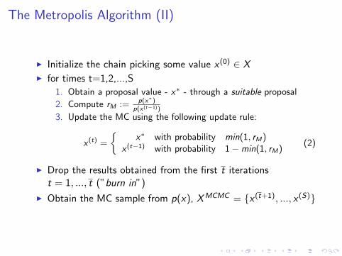
I Initialize the chain picking some value x (0) ∈ XI for times t=1,2,...,S

1. Obtain a proposal value - x∗ - through a suitable proposal

2. Compute rM := p(x∗)p(x (t−1))

3. Update the MC using the following update rule:

x (t) =

{x∗ with probability min(1, rM)

x (t−1) with probability 1−min(1, rM)(2)

I Drop the results obtained from the first t iterationst = 1, ..., t (”burn in”)

I Obtain the MC sample from p(x), XMCMC = {x (t+1), ..., x (S)}

The Metropolis Algorithm (III)

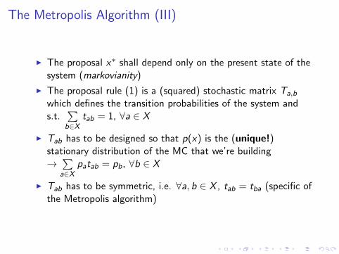
I The proposal x∗ shall depend only on the present state of thesystem (markovianity)

I The proposal rule (1) is a (squared) stochastic matrix Ta,b

which defines the transition probabilities of the system ands.t.

∑b∈X

tab = 1, ∀a ∈ X

I Tab has to be designed so that p(x) is the (unique!)stationary distribution of the MC that we’re building→∑a∈X

patab = pb, ∀b ∈ X

I Tab has to be symmetric, i.e. ∀a, b ∈ X , tab = tba (specific ofthe Metropolis algorithm)

Important Remarks on MA

First remark: the samples we obtain, won’t be uncorrelated. Still,from ergodic theory we know that they will be representative forp(x)Second remark: the acceptance ratio rM is defined only throughratios of probabilities. Due to such property, we do not need tocompute any normalization constant of the desired targetdistribution

Definition: Stationariety

Stationary (probability mass) distribution: if T is a transitionmatrix which describes a (time homogeneous) Markov chain, π is astationary (probability mass) distribution for T ifπT = π ⇒

∑a∈X

πatab = πb. Indeed π is a left-eigenvector of T

with eigen-value 1

Definition: Reversibility

Reversibility : A process (Tn)n is said to be reversible if(Tt1 ,Tt2 , ...,Ttn) has the same distribution as(Tτ−t1,Tτ−t2 , ...,Tτ−tn) for all t1, ..., tn and τ .An intuitive interpretation of the reversibility condition is that theprocess should be such that, chosen any subsequence of theprocess, the flipped version of such subsequence should come fromthe same process

Definition: Irreducibility

Irreducibility: A Markov chain T is irreducible if ∀ a, b ∈ X , thereexists some t such that T t

ab > 0. If T is time homogeneous -T tab = T τ

ab ∀t, τ - and the previous reduces to the existence ofsome path a 7→ b, ∀a, b ∈ X which has positive probability andtakes places in a finite number of transition steps

Definition: Aperiodicity

Aperiodicity: A Markov chain T is aperiodic if ∀a, b ∈ X we havegcd{t : T t

ab > 0} = 1. This implies that there is not predefinedtime-pattern for future realizations of the chain

Thm: Ergodic Thm

Ergodic Theorem: if {x (1), x (2), ...} is an irreducible1, aperiodic,and recurrent Markov chain, then there exists a unique probabilitydistribution π such that as S →∞,

I P(x (s) ∈ A)→ π(A) for any set A

I 1S

S∑s=1

g(x (s))→∫g(x)π(x)dx

Such distribution π is then the stationary distribution of theMarkov chain. Moreover π has the following property: if x (s) ∼ π,and x (s+1) is generated from the Markov chain starting at x (s),then P(x (s+1) ∈ A) = π(A) 2

1in an irreducible MC, either all states are recurrent or all are transient2in other words: once you’re sampling from π, you continue sampling from π

The Metropolis Hastings Algorithm (I)

I Detailed Balance → p(a)p(b) = tba

tab⇔ p(a)tab = p(b)tba

I Transition Matrix decomposition →

tab =

qabαab if a 6= b

1−∑j 6=a

taj if a = b(3)

where

αab :=

min

{1, p(b)

p(a)qbaqab

}if paqab > 0

1 otherwise

(4)

I Qab is another transition matrix of an arbitrary Markov chainon the states in X (transition matrix)

I αab is a conditional probability of acceptance of moves in thesystem(acceptance matrix or distribution)

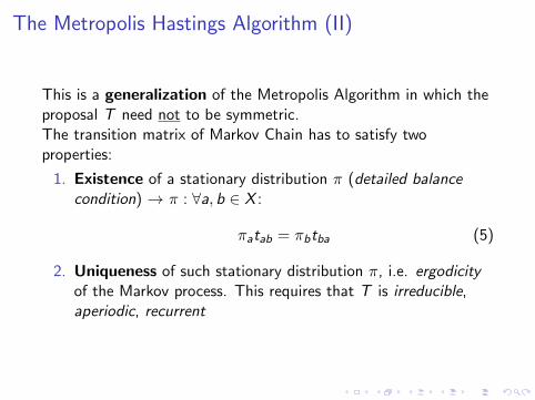
The Metropolis Hastings Algorithm (II)

This is a generalization of the Metropolis Algorithm in which theproposal T need not to be symmetric.The transition matrix of Markov Chain has to satisfy twoproperties:

1. Existence of a stationary distribution π (detailed balancecondition) → π : ∀a, b ∈ X :

πatab = πbtba (5)

2. Uniqueness of such stationary distribution π, i.e. ergodicityof the Markov process. This requires that T is irreducible,aperiodic, recurrent

The Metropolis Hastings Algorithm (III)

I Initialize the chain picking some value x0 ∈ XI for times t=1,2,...,S

1. Obtain a proposal value - x∗ - through the transition matrixQab, and specifically looking at the row QT

x t−1

2. Compute αx t−1x∗ → Hastings correction factor3. Update the MC using the following update rule:

x (t) =

{x∗ with probability αx (t−1)x∗

x (t−1) with probability 1− αx (t−1)x∗(6)

I Drop the results obtained from iterations t = 1...t

I Obtain the MC sample from p(x) as {x (t+1)...x (S)}

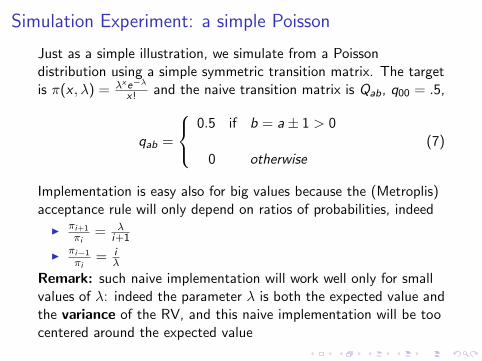
Simulation Experiment: a simple Poisson

Just as a simple illustration, we simulate from a Poissondistribution using a simple symmetric transition matrix. The targetis π(x , λ) = λxe−λ

x! and the naive transition matrix is Qab, q00 = .5,

qab =

0.5 if b = a± 1 > 0

0 otherwise(7)

Implementation is easy also for big values because the (Metroplis)acceptance rule will only depend on ratios of probabilities, indeed

I πi+1

πi= λ

i+1

I πi−1

πi= i

λ

Remark: such naive implementation will work well only for smallvalues of λ: indeed the parameter λ is both the expected value andthe variance of the RV, and this naive implementation will be toocentered around the expected value

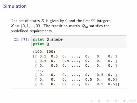
Simulation

The set of states X is given by 0 and the first 99 integers,X := {0, 1, ..., 99} The transition matrix Qab satisfies thepredefined requirements,

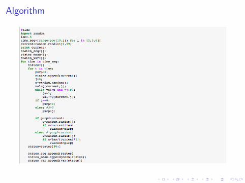
Algorithm

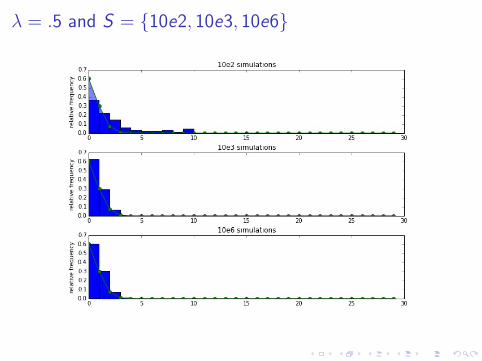
λ = .5 and S = {10e2, 10e3, 10e6}

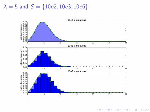
λ = 5 and S = {10e2, 10e3, 10e6}

λ = 50 and S = {10e2, 10e3, 10e6}

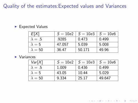
Quality of the estimates:Expected values and Variances

I Expected Values

E [X ] S = 10e2 S = 10e3 S = 10e6

λ = .5 .9285 0.473 0.499

λ = 5 47.057 5.039 5.008

λ = 50 36.47 50.171 49.96

I Variances

Var [X ] S = 10e2 S = 10e3 S = 10e6

λ = .5 1.009 0.436 0.499

λ = 5 43.05 10.44 5.029

λ = 50 9.334 25.17 49.647

Bibliography I

W. K. Hastings, Monte Carlo Sampling Methods Using Markov Chains and Their Applications,

Biometrika, Vol. 57, No. 1. (Apr., 1970), pp. 97-109

P.D. Hoff, A First Course in Bayesian Statistical Methods, Springer, chapter 10

S. Chib & E. Greenberg, Understanding the Metropolis Hastings Algorithm, The American Statistician, Vol.

49, No. 4. (Nov., 1995), pp. 327-335.