harold jeffreys's theory of probability revisited · σ-finite measure, jeffreys’s prior,...
TRANSCRIPT
arX
iv:0
804.
3173
v7 [
mat
h.ST
] 1
8 Ja
n 20
10
Statistical Science
2009, Vol. 24, No. 2, 141–172DOI: 10.1214/09-STS284c© Institute of Mathematical Statistics, 2009
Harold Jeffreys’s Theory of ProbabilityRevisitedChristian P. Robert, Nicolas Chopin and Judith Rousseau
Abstract. Published exactly seventy years ago, Jeffreys’s Theory ofProbability (1939) has had a unique impact on the Bayesian commu-nity and is now considered to be one of the main classics in BayesianStatistics as well as the initiator of the objective Bayes school. In par-ticular, its advances on the derivation of noninformative priors as wellas on the scaling of Bayes factors have had a lasting impact on the field.However, the book reflects the characteristics of the time, especially interms of mathematical rigor. In this paper we point out the fundamen-tal aspects of this reference work, especially the thorough coverage oftesting problems and the construction of both estimation and testingnoninformative priors based on functional divergences. Our major aimhere is to help modern readers in navigating in this difficult text andin concentrating on passages that are still relevant today.
Key words and phrases: Bayesian foundations, noninformative prior,σ-finite measure, Jeffreys’s prior, Kullback divergence, tests, Bayes fac-tor, p-values, goodness of fit.
Christian P. Robert is Professor of Statistics, AppliedMathematics Department, Universite Paris Dauphineand Head of the Statistics Laboratory, Center forResearch in Economics and Statistics (CREST),National Institute for Statistics and Economic Studies(INSEE), Paris, France e-mail:[email protected]. He was the President ofISBA (International Society for Bayesian Analysis) for2008. Nicolas Chopin is Professor of Statistics, ENSAE(National School for Statistics and EconomicAdministration), and Member of the StatisticsLaboratory, Center for Research in Economics andStatistics (CREST), National Institute for Statisticsand Economic Studies (INSEE), Paris, France e-mail:[email protected]. Judith Rousseau is Professorof Statistics, Applied Mathematics Department,Universite Paris Dauphine, and Member of theStatistics Laboratory, Center for Research in Economicsand Statistics (CREST), National Institute forStatistics and Economic Studies (INSEE), Paris,France e-mail: [email protected].
1Discussed in 10.1214/09-STS284E, 10.1214/09-STS284D,10.1214/09-STS284A, 10.1214/09-STS284F,10.1214/09-STS284B, 10.1214/09-STS284C; rejoinder at10.1214/09-STS284REJ.
1. INTRODUCTION
The theory of probability makes it possible torespect the great men on whose shoulders we stand.H. Jeffreys, Theory of Probability, Section 1.6.
Few Bayesian books other than Theory of Proba-bility are so often cited as a foundational text.1 Thisbook is rightly considered as the principal referencein modern Bayesian statistics. Among other innova-tions, Theory of Probability states the general princi-ple for deriving noninformative priors from the sam-pling distribution, using Fisher information. It also
This is an electronic reprint of the original articlepublished by the Institute of Mathematical Statistics inStatistical Science, 2009, Vol. 24, No. 2, 141–172. Thisreprint differs from the original in pagination andtypographic detail.
1Among the “Bayesian classics,” only Savage (1954), DeG-root (1970) and Berger (1985) seem to get more citations thanJeffreys (1939, 1948, 1961), the more recent book by Bernardoand Smith (1994) coming fairly close. The homonymous The-ory of Probability by de Finetti (1974, 1975) gets quoted athird as much (Source: Google Scholar).
1
2 C. P. ROBERT, N. CHOPIN AND J. ROUSSEAU
proposes a clear processing of Bayesian testing, in-cluding the dimension-free scaling of Bayes factors.This comprehensive treatment of Bayesian inferencefrom an objective Bayes perspective is a major inno-vation for the time, and it has certainly contributedto the advance of a field that was then submitted tosevere criticisms by R. A. Fisher (Aldrich, 2008) andothers, and was in danger of becoming a feature ofthe past. As pointed out by Zellner (1980) in his in-troduction to a volume of essays in honor of HaroldJeffreys, a fundamental strength of Theory of Prob-ability is its affirmation of a unitarian principle inthe statistical processing of all fields of science.For a 21st century reader, Jeffreys’s Theory of
Probability is nonetheless puzzling for its lack offormalism, including its difficulties in handling im-proper priors, its reliance on intuition, its long de-bate about the nature of probability, and its re-peated attempts at philosophical justifications. Thetitle itself is misleading in that there is absolutelyno exposition of the mathematical bases of probabil-ity theory in the sense of Billingsley (1986) or Feller(1970): “Theory of Inverse Probability” would havebeen more accurate. In other words, the style of thebook appears to be both verbose and often vague inits mathematical foundations for a modern reader.2
(Good, 1980, also acknowledges that many passagesof the book are “obscure.”) It is thus difficult to ex-tract from this dense text the principles that madeTheory of Probability the reference it is nowadays.In this paper we endeavor to revisit the book froma Bayesian perspective, in order to separate founda-tional principles from less relevant parts.This review is neither a historical nor a critical
exercise: while conscious that Theory of Probabil-ity reflects the idiosyncrasies both of the scientificachievements of the 1930’s—with, in particular, theemerging formalization of Probability as a branch ofMathematics against the ongoing debate on the na-ture of probabilities—and of Jeffreys’s background—as a geophysicist—, we aim rather at providing themodern reader with a reading guide, focusing on thepioneering advances made by this book. Parts thatcorrespond to the lack (at the time) of analytical(like matrix algebra) or numerical (like simulation)tools and their substitution by approximation de-vices (that are not used any longer, even though
2In order to keep readability as high as possible, we shalluse modern notation whenever the original notation is eitherunclear or inconsistent, for example, Greek letters for param-eters and roman letters for observations.
they may be surprisingly accurate), and parts thatare linked with Bayesian perspectives will be coveredfleetingly. Thus, when pointing out notions that mayseem outdated or even mathematically unsound bymodern standards, our only aim is to help the mod-ern reader stroll past them, and we apologize in ad-vance if, despite our intent, our tone seems overlypresumptuous: it is rather a reflection of our igno-rance of the current conditions at the time since (toborrow from the above quote which may sound it-self somehow presumptuous) we stand respectfullyat the feet of this giant of Bayesian Statistics.The plan of the paper follows Theory of Probabil-
ity linearly by allocating a section to each chapter ofthe book (Appendices are only mentioned through-out the paper). Section 10 contains a brief conclu-sion. Note that, in the following, words, sentencesor passages quoted from Theory of Probability arewritten in italics with no precise indication of theirlocation, in order to keep the style as light as pos-sible. We also stress that our review is based onthe third edition of Theory of Probability (Jeffreys,1961), since this is both the most matured and themost available version (through the last reprint byOxford University Press in 1998). Contemporary re-views of Theory of Probability are found in Good(1962) and Lindley (1962).
2. CHAPTER I: FUNDAMENTAL NOTIONS
The posterior probabilities of the hypotheses areproportional to the products of the prior
probabilities and the likelihoods.H. Jeffreys, Theory of Probability, Section 1.2.
The first chapter of Theory of Probability sets gen-eral goals for a coherent theory of induction. Moreimportantly, it proposes an axiomatic (if slightlytautological) derivation of prior distributions, whilejustifying this approach as coherent, compatible withthe ordinary process of learning and allowing for theincorporation of imprecise information. It also rec-ognizes the fundamental property of coherence whenupdating posterior distributions, since they can beused as the prior probability in taking into accountof a further set of data. Despite a style that is oftendifficult to penetrate, this is thus a major chapter ofTheory of Probability. It will also become clearer at alater stage that the principles exposed in this chap-ter correspond to the (modern) notion of objectiveBayes inference: despite mentions of prior probabil-ities as reflections of prior belief or existing pieces of
THEORY OF PROBABILITY REVISITED 3
information, Theory of Probability remains strictly“objective” in that prior distributions are always de-rived analytically from sampling distributions andthat all examples are treated in a noninformativemanner. One may find it surprising that a physi-cist like Jeffreys does not emphasise the appeal ofsubjective Bayes, that is, the ability to take into ac-count genuine prior information in a principled way.But this is in line with both his predecessors, in-cluding Laplace and Bayes, and their use of uniformpriors and his main field of study that he perceivedas objective (Lindley, 2008, private communication),while one of the main appeals of Theory of Probabil-ity is to provide a general and coherent frameworkto derive objective priors.
2.1 A Philosophical Exercise
The chapter starts in Section 1.0 with an epis-temological discussion of the nature of (statistical)inference. Some sections are quite puzzling. For in-stance, the example that the kinematic equation foran object in free-fall,
s= a+ ut+ 12gt
2,
cannot be deduced from observations is used as anargument against deduction under the reasoning thatan infinite number of functions,
s= a+ ut+ 12gt
2 + f(t)(t− t1) · · · (t− tn),
also apply to describe a free fall observed at timest1, . . . , tn. The limits of the epistemological discus-sion in those early pages are illustrated by the in-troduction of Ockham’s razor (the choice of the sim-plest law that fits the fact), as the meaning of whata simplest law can be remains unclear, and the sec-tion lacks a clear (objective) argument in motivatingthis choice, besides common sense, while the discus-sion ends up with a somehow paradoxical statementthat, since deductive logic provides no explanationof the choice of the simplest law, this is proof thatdeductive logic is grossly inadequate to cover scien-tific and practical requirements. On the other hand,and from a statistician’s narrower perspective, onecan re-interpret this gravity example as possibly theearliest discussion of the conceptual difficulties asso-ciated with model choice, which are still not entirelyresolved today. In that respect, it is quite fascinat-ing to see this discussion appear so early in the book(third page), as if Jeffreys had perceived how impor-tant this debate would become later.
Note that, maybe due to this very call to Ockham,the later Bayesian literature abounds in referencesto Ockham’s razor with little formalization of thisprinciple, even though Berger and Jefferys (1992),Balasubramanian (1997) and MacKay (2002) developelaborate approaches. In particular, the definitionof the Bayes factor in Section 1.6 can be seen as apartial implementation of Ockham’s razor when set-ting the probabilities of both models equal to 1/2.In the beginning of his Chapter 28, entitled ModelChoice and Occam’s Razor, MacKay (2002) arguesthat Bayesian inference embodies Ockham’s razorbecause “simple” models tend to produce more pre-cise predictions and, thus, when the data is equallycompatible with several models, the simplest onewill end up as the most probable. This is generallytrue, even though there are some counterexamplesin Bayesian nonparametrics.Overall, we nonetheless feel that this part of The-
ory of Probability could be skipped at first read-ing as less relevant for Bayesian studies. In particu-lar, the opposition between mathematical deductionand statistical induction does not appear to carry astrong argument, even though the distinction needs(needed?) to be made for mathematically orientedreaders unfamiliar with statistics. However, from ahistorical point of view, this opposition must be con-sidered against the then-ongoing debate about thenature of induction, as illustrated, for instance, byKarl Popper’s articles of this period about the logi-cal impossibility of induction (Popper, 1934).
2.2 Foundational Principles
The text becomes more focused when dealing withthe construction of a theory of inference: while somenotions are yet to be defined, including the pervasiveevidence, sentences like inference involves in its verynature the possibility that the alternative chosen asthe most likely may in fact be wrong are in line withour current interpretation of modeling and obviouslywith the Bayesian paradigm. In Section 1.1 Jeffreyssets up a collection of postulates or rules that actlike axioms for his theory of inference, some of whichrequire later explanations to be fully understood:
1. All hypotheses must be explicitly stated and theconclusions must follow from the hypotheses: whatmay first sound like an obvious scientific principleis in fact a leading characteristic of Bayesian statis-tics. While it seems to open a whole range of new
4 C. P. ROBERT, N. CHOPIN AND J. ROUSSEAU
questions—“To what extent must we define our be-lief in the statistical models used to build our in-ference? How can a unique conclusion stem from agiven model and a given set of observations?”—andwhile it may sound far too generic to be useful, wemay interpret this statement as setting the workingprinciple of Bayesian decision theory: given a prior,a sampling distribution, an observation and a lossfunction, there exists a single decision procedure.In contrast, the frequentist theories of Neyman orof Fisher require the choice of ad hoc procedures,whose (good or bad) properties they later analyze.But this may be a far-fetched interpretation of thisrule at this stage even though the comment will ap-pear more clearly later.2. The theory must be self-consistent. The state-
ment is somehow a repetition of the previous ruleand it is only later (in Section 3.10) that its mean-ing becomes clearer, in connection with the intro-duction of Jeffreys’s noninformative priors as a self-contained principle. Consistency is nonetheless a dom-inant feature of the book, as illustrated in Section 3.1with the rejection of Haldane’s prior.3
3. Any rule must be applicable in practice. This“rule” does not seem to carry any weight in prac-tice. In addition, the explicit prohibition of esti-mates based on impossible experiments sounds im-plementable only through deductive arguments. Butthis leads to the exclusion of rules based on fre-quency arguments and, as such, is fundamental insetting a Bayesian framework. Alternatively (andthis is another interpretation), this constraint shouldbe worded in more formal terms of the measurabilityof procedures.4. The theory must provide explicitly for the pos-
sibility that inferences made by it may turn out tobe wrong. This is both a fundamental aspect of sta-tistical inference and an indication of a surprisingview of inference. Indeed, even when conditioningon the model, inference is never right in the sensethat a point estimate rarely gives the true answer.It may be that Jeffreys is solely thinking of sta-tistical testing, in which case the rightfulness of adecision is necessarily conditional on the truthful-ness of the corresponding model and thus dubious.A more relative (or more precise) statement would
3Consistency is then to be understood in the weak sense ofinvariant under reparameterization, which is a usual argumentfor Jeffreys’s principle, not in terms of asymptotic convergenceproperties.
have been more adequate. But, from reading fur-ther (as in Section 1.2), it appears that this rule isto be understood as the foundational principle (thechief constructive rule) for defining prior distribu-tions. While this is certainly not clear at this stage,Bayesian inference does indeed provide for the pos-sibility that the model under study is not correctand for the unreliability of the resulting inferencevia a posterior probability.5. The theory must not deny any empirical propo-
sition a priori. This principle remains unclear whenput into practice. If it is to be understood in thesense of a physical theory, there is no reason whysome empirical proposition could not be excludedfrom the start. If it is the sense of an inferentialtheory, then the statement would require a betterdefinition of empirical proposition. But Jeffreys us-ing the epithet a priori seems to imply that the priordistribution corresponding to the theory must be asinclusive as possible. This certainly makes sense aslong as prior information does not exclude parts ofthe parameter space as, for instance, in Physics.6. The number of postulates should be reduced to a
minimum. This rule sounds like an embedded Ock-ham’s razor, but, more positively, it can also be in-terpreted as a call for noninformative priors. Onceagain, the vagueness of the wording opens a widerange of interpretations.7. The theory need not represent thought-processes
in details, but should agree with them in outline.This vague principle could be an attempt at rec-onciliating statistical theories, but it does not giveclear directions on how to proceed. In the light ofJeffreys’s arguments, it could rather signify that theconstruction of prior distributions cannot exactly re-flect an actual construction in real life. Since a non-informative (or “objective”) perspective is adoptedfor most of the book, this is more likely to be a pre-liminary argument in favor of this line of thought. InSection 1.2 this rule is invoked to derive the (prior)ordering of events.8. An objection carries no weight if [it] would in-
validate part of pure mathematics. This rule groundsTheory of Probability within mathematics, which maybe a necessary reminder in the spirit of the time(where some were attempting to dissociate statis-tics from mathematics).
The next paragraph discusses the notion of prob-ability. Its interest is mostly historical: in the early1930’s, the axiomatic definition of probability based
THEORY OF PROBABILITY REVISITED 5
on Kolmogorov’s axioms was not yet universally ac-cepted, and there were still attempts to base thisdefinition on limiting properties. In particular,Lebesgue integration was not part of the undergrad-uate curriculum till the late 1950’s at either Cam-bridge or Oxford (Lindley, 2008, private communi-cation). This debate is no longer relevant, and thecurrent theory of probability, as derived from mea-sure theory, does not bear further discussion. Thisalso removes the ambiguity of constructing objectiveprobabilities as derived from actual or possible ob-servations. A probability model is to be understoodas a mathematical (and thus unobjectionable) con-struct, in agreement with Rule 8 above.Then follows (still in Section 1.1) a rather long
debate on causality versus determinism. While theprinciples stated in those pages are quite accept-able, the discussion only uses the most basic conceptof determinism, namely, that identical causes giveidentical effects, in the sense of Laplace. We thusagree with Jeffreys that, at this level, the principleis useless, but the same paragraph actually leavesus quite confused as to its real purpose. A likely ex-planation (Lindley, 2008, personal communication)is that Jeffreys stresses the inevitability of probabil-ity statements in Science: (measurement) errors arenot mistakes but part of the picture.
2.3 Prior Distributions
In Section 1.2 Jeffreys introduces the notion ofprior in an indirect way, by considering that theprobability of a proposition is always conditional onsome data and that the occurrence of new items ofinformation (new evidence) on this proposition sim-ply updates the available data. This is slightly con-trary to our current way of defining a prior distri-bution π on a parameter θ as the information avail-able on θ prior to the observation of the data, butit simply conveys the fact that the prior distribu-tion must be derived from some prior items of in-formation about θ. As pointed out by Jeffreys, thisalso allows for the coexistence of prior distributionsfor different experts within the same probabilisticframework.4 In the sequel all statements will, how-ever, condition on the same data.The following paragraphs derive standard math-
ematical logic axioms that directly follow from a
4Jeffreys seems to further note that the same conditioningapplies for the model of reference.
formal (modern) definition of a probability distri-bution, with the provision that this probability isalways conditional on the same data. This is alsoreminiscent of the derivation of the existence of aprior distribution from an ordering of prior proba-bilities in DeGroot (1970), but the discussion aboutthe arbitrary ranking of probabilities between 0 and1 may sound anecdotal today. Note also that, froma mathematical point of view, defining only condi-tional probabilities like P (p|q) is somehow superflu-ous in that, if the conditioning q is to remain fixed,P (·|q) is a regular probability distribution, while, ifq is to be updated into qr, P (·|qr) can be derivedfrom P (·|q) by Bayes’ theorem (which is to be in-troduced later). Therefore, in all cases, P (·|q) ap-pears like the reference probability. At some stage,while stating that the probability of the sure eventis equal to one is merely a convention, Jeffreys indi-cates that, when expressing ignorance over an infi-nite range of values of a quantity, it may be conve-nient to use ∞ instead. Clearly, this paves the wayfor the introduction of improper priors.5 Unfortu-nately, the convention and the motivation (to keepratios for finite ranges determinate) do not seemcorrect, if in tune with the perspective of the time(see, e.g., Lhoste, 1923; Broemeling and Broemel-ing, 2003). Notably, setting all events involving aninfinite range with a probability equal to ∞ seemsto restrict the abilities of the theory to a far ex-tent.6 Similar to Laplace, Jeffreys is more used tohandling equal probability finite sets than continu-ous sets and the extension to continuous settings isunorthodox, using, for instance, Dedekind’s sectionsand putting several meanings under the notation dx.Given the convoluted derivation of conditional prob-abilities in this context, the book states the productrule P (qr|p) = P (q|p)P (r|qp) as an axiom, ratherthan as a consequence of the basic probability ax-ioms. It leads (in Section 1.22) to Bayes’ theorem,
5Jeffreys’s Theory of Probability strongly differs from theearlier Scientific Inference (1931) in this respect, the latter be-ing rather dismissive of the mathematical difficulty: To makethis integral equal to 1 we should therefore have to includea zero factor unless very small and very large values are ex-cluded. This does appear to be the case (Section 5.43, page67).
6This difficulty with handling σ-finite measures and contin-uous variables will be recurrent throughout the book: Jeffreysdoes not seem to be adverse to normalizing an improper dis-tribution by ∞, even though the corresponding derivationsare not meaningful.
6 C. P. ROBERT, N. CHOPIN AND J. ROUSSEAU
namely, that, for all events qr,
P (qr|pH)∝ P (qr|H)P (p|qrH),
where H denotes the information available and p aset of observations. In this (modern) format P (p|qrH)is identified as Fisher likelihood and P (qr|H) as theprior probability. Bayes’ theorem is defined as theprinciple of inverse probability and only for finitesets, rather than for measures.7 Obviously, the gen-eral version of Bayes’ theorem is used in the sequelfor continuous parameter spaces.Section 1.3 represents one of the few forays of
the book into the realm of decision theory,8 in con-nection with Laplace’s notions of mathematical andmoral expectations, and with Bernoulli’s Saint Pe-tersburg paradox, but there is no recognition of thecentral role of the loss function in defining an opti-mal Bayes rule as formalized later by Wald (1950)and Raiffa and Schlaifer (1961). The attribution ofa decision-theoretic background to T. Bayes himselfis surprising, since there is not anything close to thenotion of loss or of benefit in Bayes’ (1763) origi-nal paper. We nonetheless find there the seed of anidea later developed in Rubin (1987), among oth-ers, that prior and loss function are indistinguish-able. [Section 1.8 briefly re-enters this perspectiveto point out that (posterior) expectations are oftennowhere near the actual value of the random quan-tity.] The next section (Section 1.4) is important inthat it tackles for the first time the issue of nonin-formative priors. When the number of alternativesis finite, Jeffreys picks the uniform prior as his non-informative prior, following Laplace’s Principle ofInsufficient Reason. The difficulties associated withthis choice in continuous settings are not mentionedat this stage.
2.4 More Axiomatics and Some Asymptotics
Section 1.5 attempts an axiomatic derivation thatthe Bayesian principles just stated follow the rules
7As noted by Fienberg (2006), the adjective term“Bayesian” had not yet appeared in the statistical literatureby the time Theory of Probability was published, and Jeffreyssticks to the 19th century denomination of “inverse probabil-ity.” The adjective can be traced back to either Ronald Fisher,who used it in a rather derogatory meaning, or to AbrahamWald, who gave it a more complimentary meaning in Wald(1950).
8The reference point estimator advocated by Jeffreys (ifany) seems to be the maximum a posteriori (MAP) estimator,even though he stated in his discussion of Lindley (1953) thathe deprecated the whole idea of picking out a unique estimate.
imposed earlier. This part does not bring much nov-elty, once the fundamental properties of a proba-bility distribution are stated. This is basically thepurpose of this section, where earlier “Axioms” arechecked in terms of the posterior probability P (·|pH).A reassuring consequence of this derivation is thatthe use of a posterior probability as the basis forinference cannot lead to inconsistency. The use ofthe posterior as a new prior for future observationsand the corresponding learning principle are devel-oped at this stage. The debate about the choice ofthe prior distribution is postponed till later, whilethe issue of the influence of this prior distributionis dismissed as having very little difference [on] theresults, which needs to be quantified, as in the quotebelow at the beginning of Section 5.Given the informal approach to (or rather with-
out) measure theory adopted in Theory of Probabil-ity, the study of the limiting behavior of posteriordistributions in Section 1.6 does not provide muchinsight. For instance, the fact that
P (q|p1 · · ·pnH)
=P (q|H)
P (p1|H)P (p2|p1H) · · ·P (pn|p1 · · ·pn−1H)
is shown to induce that P (pn|p1 · · ·pn−1H) convergesto 1 is not particularly surprising, although it relatesto Laplace’s principle that repeated verifications ofconsequences of a hypothesis will make it practicallycertain that the next consequence will be verified. Itwould have been equally interesting to focus on casesin which P (q|p1 · · ·pnH) goes to 1.The end of Section 1.62 introduces some quanti-
ties of interest, such as the distinction between esti-mation problems and significance tests, but with noclear guideline: when comparing models of complex-ity m (this quantity being only defined for differen-tial equations), Jeffreys suggests using prior prob-abilities that are penalized by m, such as 2−m or6/π2m2, the motivation for those specific values be-ing that the corresponding series converge. Penal-ization by the model complexity is quite an inter-esting idea, to be formalized later by, for example,Rissanen (1983, 1990), but Jeffreys somehow killsthis idea before it is hatched by pointing out thedifficulties with the definition of m.Instead, Jeffreys switches to a completely different
(if paramount) topic by defining in a few lines theBayes factor for testing a point null hypothesis,
K =P (q|θH)
P (q′|θH)
/ P (q|H)
P (q′|H),
THEORY OF PROBABILITY REVISITED 7
where θ denotes the data. He suggests using P (q|H) =1/2 as a default value, except for sequences of em-bedded hypotheses for which he suggests
P (q|H)
P (q′|H)= 2,
presumably because the series with leading term 2−n
is converging.Once again, the rather quick coverage of this ma-
terial is somehow frustrating, as further justifica-tions would have been necessary for the choice ofthe constant and so on.9 Instead, the chapter con-cludes with a discussion of the distinction between“idealism” and “realism” that can be skipped formost purposes.
3. CHAPTER II: DIRECT PROBABILITIES
The whole of the information contained in theobservations that is relevant to the posterior
probabilities of different hypotheses is summedup in the values that they give to the likelihood.
H. Jeffreys, Theory of Probability, Section 2.0.
This chapter is certainly the least “Bayesian” chap-ter of the book, since it covers both the standardsampling distributions and some equally standardprobability results. It starts with a reminder thatthe principle of inverse probability can be stated inthe form
Posterior Probability ∝ Prior Probability
· Likelihood ,thus rephrasing Bayes’ theorem in terms of the like-lihood and with the proper indication that the rel-evant information contained in the observations issummarized by the likelihood (sufficiency will bementioned later in Section 3.7). Then follows (stillin Section 2.0) a long paragraph about the tenta-tive nature of models, concluding that a statisticalmodel must be made part of the prior informationH before it can be tested against the observations,which (presumably) relates to the fact that Bayesian
9Similarly, the argument against philosophers that main-tain that no method based on the theory of probability can givea (...) non-zero probability to a precise value against a contin-uous background is not convincing as stated. The distinctionbetween zero measure events and mixture priors including aDirac mass should have been better explained, since this isthe basis for Bayesian point-null testing.
model assessment must involve a description of thealternative(s) to be validated.The main bulk of the chapter is about sampling
distributions. Section 2.1 introduces binomial andhypergeometric distributions at length, including theinteresting problem of deciding between binomialversus negative binomial experiments when facedwith the outcome of a survey, used later in the de-fence of the Likelihood Principle (Berger andWolpert,1988). The description of the binomial contains theequally interesting remark that a given coin repeat-edly thrown will show a bias toward head or tail dueto the wear, a remark later exploited in Diaconis andYlvisaker (1985) to justify the use of mixtures ofconjugate priors. Bernoulli’s version of the CentralLimit theorem is also recalled in this section, withno particular appeal if one considers that a mod-ern Statistics course (see, e.g., Casella and Berger,2001) would first start with the probabilistic back-ground.10
The Poisson distribution is first introduced as alimiting distribution for the binomial distributionB(n,p) when n is large and np is bounded. (Connec-tions with radioactive disintegration are mentionedafterward.) The normal distribution is proposed asa large sample approximation to a sum of Bernoullirandom variables. As for the other distributions,there is some attempt at justifying the use of thenormal distribution, as well as [what we find to be]a confusing paragraph about the “true” and “actualobserved” values of the parameters. A long section(Section 2.3) expands about the properties of Pear-son’s distributions, then allowing Jeffreys to intro-duce the negative binomial as a mixture of Poissondistributions. The introduction of the bivariate nor-mal distribution is similarly convoluted, using firstbinomial variates and second a limiting argument,and without resorting to matrix formalism.Section 2.6 attempts to introduce cumulative dis-
tribution functions in a more formal manner, usingthe current three-step definition, but again dealingwith limits in an informal way. Rather coherentlyfrom a geophysicist’s point of view, characteristicfunctions are also covered in great detail, includingconnections with moments and the Cauchy distribu-tion, as well as Levy’s inversion theorem. The main
10In fact, some of the statements in Theory of Probabilitythat surround the statement of the Central Limit theorem arenot in agreement with measure theory, as, for instance, theconfusion between pointwise and uniform convergence, andconvergence in probability and convergence in distribution.
8 C. P. ROBERT, N. CHOPIN AND J. ROUSSEAU
goal of using characteristic functions seems nonethe-less to be able to establish the Central Limit theo-rem in its full generality (Section 2.664).Rather surprisingly for a Bayesian reference book
and mostly in complete disconnection with the test-ing chapters, the χ2 test of goodness of fit is given alarge and uncritical place within this book, includ-ing an adjustment for the degrees of freedom.11 Ex-amples include the obvious independence of a rect-angular contingency table. The only criticism (Sec-tion 2.76) is fairly obscure in that it blames poorperformances of the χ2 test on the fact that all di-vergences in the χ2 sum are equally weighted. Thetest is nonetheless implemented in the most classi-cal manner, namely, that the hypothesis is rejectedif the χ2 statistic is outside the standard interval.It is unclear from the text in Section 2.76 that re-jection would occur were the χ2 statistic too small,even though Jeffreys rightly addresses the issue atthe end of Chapter 5 (Section 5.63). He also men-tions the need to coalesce small groups into groupsof size at least 5 with no further justification. Thechapter concludes with similar uses of Student’s tand Fisher’s z tests.
4. CHAPTER III: ESTIMATION PROBLEMS
If we have no information relevant to the actualvalue of the parameter, the probability must be
chosen so as to express the fact that we have none.H. Jeffreys, Theory of Probability, Section 3.1.
This is a major chapter of Theory of Probabil-ity as it introduces both exponential families andthe principle of Jeffreys noninformative priors. Themain concepts are already present in the early sec-tions, including some invariance principles. The pur-pose of the chapter is stated as a point estimationproblem, where obtaining the probability distribu-tion of [the] parameters, given the observations isthe goal. Note that estimation is not to be under-stood in the (modern?) sense of point estimation,that is, as a way to produce numerical substitutesfor the true parameters that are based on the data,
11Interestingly enough, the parameters are estimated byminimum χ2 rather than either maximum likelihood orBayesian point estimates. This is, again, a reflection of thepractice of the time, coupled with the fact that most ap-proaches are asymptotically indistinguishable. Posterior ex-pectations are not at all advocated as Bayes (point) estima-tors in Theory of Probability.
since the decision-theoretic perspective for building(point) estimators is mostly missing from the book(see Section 1.8 for a very brief remark on expecta-tions). Both Good (1980) and Lindley (1980) stressthis absence.
4.1 Noninformative Priors of Former Days
Section 3.1 sets the principles for selecting nonin-formative priors. Jeffreys recalls Laplace’s rule that,if a parameter is real-valued, its prior probabilityshould be taken as uniformly distributed, while, ifthis parameter is positive, the prior probability of itslogarithm should be taken as uniformly distributed.The motivation advanced for using both priors isthe invariance principle, namely, the invariance ofthe prior selection under several different sets of pa-rameters. At this stage, there is no recognition ofa potential problem with using a σ-finite measureand, in particular, with the fact that these priorsare not probability distributions, but rather a sim-ple warning that these are formal rules expressingignorance. We face the difficulty mentioned earlierwhen considering σ-finite measures since they arenot properly handled at this stage: when statingthat one starts with any distribution of prior proba-bility, it is not possible to include σ-finite measuresthis way, except via the [incorrect] argument that aprobability is merely a number and, thus, that thetotal weight can be ∞ as well as 1: use ∞ insteadof 1 to indicate certainty on data H . The wrong in-terpretation of a σ-finite measure as a probabilitydistribution (and of ∞ as a “number”) then leadsto immediate paradoxes, such as the prior proba-bility of any finite range being null, which soundsinconsistent with the statement that we know noth-ing about the parameter, but this results from anover-interpretation of the measure as a probabilitydistribution already pointed out by Lindley (1971,1980) and Kass and Wasserman (1996).The argument for using a flat (Lebesgue) prior is
based (a) on its use by both Bayes and Laplace infinite or compact settings, and (b) on the argumentthat it correctly reflects the absence of prior knowl-edge about the value of the parameter. At this stage,no point is made against it for reasons related withthe invariance principle—there is only one parame-terization that coincides with a uniform prior—butJeffreys already argues that flat priors cannot beused for significance tests, because they would al-ways reject the point null hypothesis. Even thoughBayesian significance tests, including Bayes factors,
THEORY OF PROBABILITY REVISITED 9
have not yet been properly introduced, the notionof an infinite mass canceling a point null hypothesisis sufficiently intuitive to be used at this point.While, indeed, using an improper prior is a ma-
jor difficulty when testing point null hypotheses be-cause it gives an infinite mass to the alternative(DeGroot, 1970), Jeffreys fails to identify the prob-lem as such but rather blames the flat prior appliedto a parameter with a semi-infinite range of pos-sible values. He then goes on justifying the use ofπ(σ) = 1/σ for positive parameters (replicating theargument of Lhoste, 1923) on the basis that it isinvariant for the change of parameters = 1/σ, aswell as any other power, failing to recognize thatother transforms that preserve positivity do not ex-hibit such an invariance. One has to admit, however,that, from a physicist’s perspective, power trans-forms are more important than other mathematicaltransforms, such as arctan, because they can be as-signed meaningful units of measurement, while otherfunctions cannot. At least this seems to be the spiritof the examples considered in Theory of Probability :Some methods of measuring the charge of an elec-tron give e, others e2.There is a vague indication that Jeffreys may also
recognize π(σ) = 1/σ as the scale group invariantmeasure, but this is unclear. An indefensible argu-ment follows, namely, that
∫ a
0vn dv
/
∫ ∞
avn dv
is only indeterminate when n=−1, which allows usto avoid contradictions about the lack of prior in-formation. Jeffreys acknowledges that this does notsolve the problem since this choice implies that theprior “probability” of a finite interval (a, b) is thenalways null, but he avoids the difficulty by admit-ting that the probability that σ falls in a particu-lar range is zero, because zero probability does notimply impossibility. He also acknowledges that theinvariance principle cannot encompass the wholerange of transforms without being inconsistent, buthe nonetheless sticks to the π(σ) = 1/σ prior as itis better than the Bayes–Laplace rule.12 Once again,the argument sustaining the whole of Section 3.1 is
12In both the 19th and early 20th centuries, there is a tra-dition within the not-yet-Bayesian literature to go to extremelengths in the justification of a particular prior distribution, asif there existed one golden prior. See, for example, Broemelingand Broemeling (2003) in this respect.
incomplete since missing the fundamental issue ofdistinguishing proper from improper priors.While Haldane’s (1932) prior on probabilities (or
rather on chances as defined in Section 1.7),
π(p)∝ 1
p(1− p),
is dismissed as too extreme (and inconsistent), thereis no discussion of the main difficulty with this prior(or with any other improper prior associated with afinite-support sampling distribution), which is thatthe corresponding posterior distribution is not de-fined when x ∼ B(n,p) is either equal to 0 or to n(although Jeffreys concludes that x = 0 leads to apoint mass at p = 0, due to the infinite mass nor-malization).13 Instead, the corresponding Jeffreys’sprior
π(p)∝ 1√
p(1− p)
is suggested with little justification against the (truly)uniform prior: we may as well use the uniform dis-tribution.
4.2 Laplace’s Succession Rule
Section 3.2 contains a Bayesian processing ofLaplace’s succession rule, which is an easy introduc-tion given that the parameter of the sampling dis-tribution, a hypergeometric H(N,r), is an integer.The choice of a uniform prior on r, π(r) = 1/(N+1),does not require much of a discussion and the pos-terior distribution
π(r|l,m,N,H) =
(
rl
)(
N − rm
)
/
(
N +1l+m+ 1
)
is available in closed form, including the normal-izing constant. The posterior predictive probabilitythat the next specimen will be of the same type isthen (l+1)/(l+m+1) and more complex predictiveprobabilities can be computed as well. As in earlierbooks involving Laplace’s succession rule, the sec-tion argues about its truthfulness from a metaphys-ical point of view (using classical arguments about
13Jeffreys (1931, 1937) does address the problem in aclearer manner, stating that this is not serious, for so longas the sample is homogeneous (meaning x = 0, n) the ex-treme values (meaning p = 0,1) are still admissible, and wedo attach a high probability to the proposition is of one type;while as soon as any exceptions are known the extreme valuesare completely excluded and no infinity arises (Section 10.1,page 195).
10 C. P. ROBERT, N. CHOPIN AND J. ROUSSEAU
the probabilities that the sun rising tomorrow andthat all swans are white that always seem to be as-sociates themselves with this topic) but, more inter-estingly, it then moves to introducing a point masson specific values of the parameter in preparationfor hypothesis testing. Namely, following a renewedcriticism of the uniform assessment via the fact that
P (r =N |l,m= 0,N,H)
P (r 6=N |l= n,N,H)=
l+ 1
N + 1
is too small, Jeffreys suggests setting aside a portion2k of the prior mass for both extreme values r = 0and r=N . This is indeed equivalent to using a pointmass on the null hypothesis of homogeneity of thepopulation. While mixed samples are independentof the choice of k (since they exclude those extremevalues), a sample of the first type with l = n leadsto a posterior probability ratio of
P (r =N |l= n,N,H)
P (r 6=N |l= n,N,H)=n+ 1
N − n
k
1− 2k
N − 1
1,
which leads to the crucial question of the choice14 ofk. The ensuing discussion is not entirely convincing:12 is too large, 1
4 is not unreasonable [but] too low inthis case. The alternative
k =1
4+
1
N +1
argues that the classification of possibilities [is] asfollows: (1) Population homogeneous on account ofsome general rule. (2) No general rule but extremevalues to be treated on a level with others. This pro-posal is mostly interesting for its bearing on thecontinuous case, for, in the finite case, it does notsound logical to put weight on the null hypothesis(r = 0 and r =N ) within the alternative, since thisconfuses the issue. (See Berger, Bernardo and Sun,2009, for a recent reappraisal of this approach fromthe point of view of reference priors.)Section 3.3 seems to extend Laplace’s succession
rule to the case in which the class sampled consistsof several types, but it actually deals with the (muchmore interesting) case of Bayesian inference for themultinomial M(n;p1, . . . , pr) distribution, when us-ing the Dirichlet D(1, . . . ,1) distribution as a prior.Jeffreys recovers the Dirichlet D(x1 + 1, . . . , xr + 1)
14A prior weight of 2k = 1/2 is reasonable since it givesequal probability to both hypotheses.
distribution as the posterior distribution and he de-rives the predictive probability that the next memberwill be of the first type as
(x1 +1)/∑
i
xi + r.
There could be some connections there with the ir-relevance of alternative hypotheses later (in time)discussed in polytomous regression models (Gourierouxand Monfort, 1996), but they are well hidden. In anycase, the Dirichlet distribution is not invariant to theintroduction of new types.
4.3 Poisson Distribution
The processing of the estimation of the parameterα of the Poisson distribution P(α) is based on the[improper] prior π(α)∝ 1/α, deemed to be the cor-rect prior probability distribution for scale invariancereasons. Given n observations from P(α) with sumSn, Jeffreys reproduces Haldane’s (1932) derivationof the Gamma posterior Ga(Sn, n) and he notes thatSn is a sufficient statistic, but does not make a gen-eral property of it at this stage. (This is done inSection 3.7.)The alternative choice π(α) ∝ 1/
√α will be later
justified in Section 3.10 not as Jeffreys’s (invariant)prior but as leading to a posterior defined for allobservations, which is not the case of π(α) ∝ 1/αwhen x= 0, a fact overlooked by Jeffreys. Note thatπ(α)∝ 1/α can nonetheless be advocated by Jeffreyson the ground that the Poisson process derives fromthe exponential distribution, for which α is a scaleparameter: e−αt represents the fraction of the atomsoriginally present that survive after time t.
4.4 Normal Distribution
When the sampling variance σ2 of a normal modelN (µ,σ2) is known, the posterior distribution associ-ated with a flat prior is correctly derived as µ|x1, . . . ,xn ∼N (x, σ2/n) (with the repeated difficulty aboutthe use of a σ-finite measure as a probability). Underthe joint improper prior
π(µ,σ)∝ 1/σ,
the (marginal) posterior on µ is obtained as a Stu-dent’s t
T (n− 1, x, s2/n(n− 1))
distribution, while the marginal posterior on σ2 isan inverse gamma IG((n− 1)/2, s2/2).15
15Section 3.41 also contains the interesting remark that,conditional on two observations, x1 and x2, the posterior
THEORY OF PROBABILITY REVISITED 11
Jeffreys notices that, when n= 1, the above priordoes not lead to a proper posterior since π(µ|x1)∝1/|µ − x1| is not integrable, but he concludes thatthe solution degenerates in the right way, which, wesuppose, is meant to say that there is not enoughinformation in the data. But, without further for-malization, it is a delicate conclusion to make.Under the same noninformative prior, the predic-
tive density of a second sample with sufficient statis-tic (x2, s2) is found
16 to be proportional to
{
n1s21 + n2s
22 +
n1n2n1 + n2
(x2 − x1)2
}−(n1+n2−1)/2
.
A direct conclusion is that this implies that x2 ands2 are dependent for the predictive, if independentgiven µ and σ, while the marginal predictives on x2and s22 are Student’s t and Fisher’s z, respectively.Extensions to the prediction of multiple future sam-ples with the same (Section 3.43) or with different(Section 3.44) means follow without surprise. In thelatter case, given m samples of nr (1≤ r ≤m) nor-mal N (µi, σ
2) measurements, the posterior on σ2
under the noninformative prior
π(µ1, . . . , µr, σ)∝ 1/σ
is again an inverse gamma IG(ν/2, s2/2) distribu-tion,17 with s2 =
∑
r
∑
i(xri − xr)2 and ν =
∑
r nr,while the posterior on t=
√ni(µi − xi)/s is a Stu-
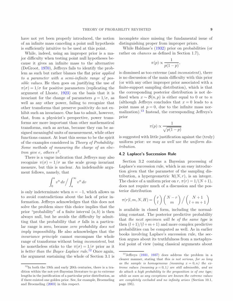
dent’s t with ν degrees of freedom for all i’s (nomatter what the number of observations within thisgroup is). Figure 1 represents the posteriors on themeans µi for the data set analyzed in this section onseven sets of measurements of the gravity. A para-
probability that µ is between both observations is exactly 1/2.Jeffreys attributes this property to the fact that the scale σ isdirectly estimated from those two observations under a nonin-formative prior. Section 3.8 generalizes the observation to alllocation-scale families with median equal to the location. Oth-erwise, the posterior probability is less than 1/2. Similarly, theprobability that a third observation x3 will be between x1 andx2 is equal to 1/3 under the predictive. While Jeffreys givesa proof by complete integration, this is a direct consequenceof the exchangeability of x1, x2 and x3. Note also that this isone of the rare occurrences of a credible interval in the book.
16In the current 1961 edition, n2s22 is mistakenly typed as
n22s
22 in equation (6) of Section 3.42.
17Jeffreys does not use the term “inverse gamma distribu-tion” but simply notes that this is a distribution with a scaleparameter that is given by a single set of tables (for a given ν).He also notices that the distribution of the transform log(σ/s)is closer to a normal distribution than the original.
Fig. 1. Seven posterior distributions on the values of accel-eration due to gravity (in cm/sec2) at locations in East Africawhen using a noninformative prior.
graph in Section 3.44 contains hints about hierar-chical Bayes modeling as a way of strengthening es-timation, which is a perspective later advanced infavor of this approach (Lindley and Smith, 1972;Berger and Robert, 1990).The extension in Section 3.5 to the setting of the
normal linear regression model should be simple (see,e.g., Marin and Robert, 2007, Chapter 3), exceptthat the use of tensorial conventions—like when asuffix i is repeated it is to be given all values from 1to m—and the absence of matrix notation makes thereading quite arduous for today’s readers.18 Becauseof this lack of matrix tools, Jeffreys uses an implicitdiagonalization of the regressor matrix XTX (withmodern notation) and thus expresses the posteriorin terms of the transforms ξi of the regression co-efficients βi. This section is worth reading if onlyto realize the immense advantage of using matrixnotation. The case of regression equations
yi =Xiβ + εi, εi ∼N (0, σ2i ),
with different unknown variances leads to a poly-t output (Bauwens, 1984) under a noninformativeprior, which is deemed to be a complication, andJeffreys prefers to revert to the case when σ2i = ωiσ
2
with known ωi’s.19 The final part of this section
18Using the notation ci for yi, xi for βi, yi for βi and air
for xir certainly makes reading this part more arduous.19Sections 3.53 and 3.54 detail the numerical resolution of
the normal equations by iterative methods and have no realbearing on modern Bayesian analysis.
12 C. P. ROBERT, N. CHOPIN AND J. ROUSSEAU
mentions the interesting subcase of estimating a nor-mal mean α when truncated at α = 0: negative ob-servations do not need to be rejected since only theposterior distribution has to be truncated in 0. [Ina similar spirit, Section 3.6 shows how to process auniform U(α−σ,α+σ) distribution under the non-informative π(α,σ) = 1/σ prior.]Section 3.9 examines the estimation of a two-dimen-
sional covariance matrix
Θ =
(
σ2 στστ τ2
)
under centred normal observations. The prior advo-cated by Jeffreys is π(τ, σ, )∝ 1/τσ, leading to the(marginal) posterior
π(| ˆ, n)
∝∫ ∞
0
(1− 2)n/2
(coshβ − ˆ)ndβ
=(1− 2)n/2
(1− ˆ)n−1/2
·∫ 1
0
(1− u)n−1
√2u
{1− (1 + ˆ)u/2}−1/2 du
that only depends on ˆ. (Jeffreys notes that, when σand τ are known, the posterior of also depends onthe empirical variances for both components. Thisparadoxical increase in the dimension of the suffi-cient statistics when the number of parameters is de-creasing is another illustration of the limited mean-ing of marginal sufficient statistics pointed out byBasu, 1988.) While this integral can be computedvia confluent hypergeometric functions (Gradshteynand Ryzhik, 1980),
∫ 1
0
(1− x)n−1
√
u(1− au)du
=B(1/2, n)2F1{1/2,1/2;n+ 1/2; (1 + ˆ)/2},the corresponding posterior is certainly less manage-able than the inverse Wishart that would result froma power prior |Θ|γ on the matrix Θ itself. The ex-tension to noncentred observations with flat priorson the means induces a small change in the outcomein that
π(| ˆ, n)∝ (1− 2)(n−1)/2
(1− ˆ)n−3/2
·∫ 1
0
(1− u)n−2
√2u
· {1− (1 + ˆ)u/2}−1/2 du,
which is also the posterior obtained directly from thedistribution of ˆ. Indeed, the sampling distributionis given by
f(ˆ|) = n− 2√2π
(1− ˆ2)(n−4)/2
· (1− 2)(n−1)/2 Γ(n− 1)
Γ(n− 1/2)
· (1− ˆ)−(n−3/2)
· 2F1{1/2,1/2;n− 1/2; (1 + ˆ)/2}.There is thus no marginalization paradox (Dawid,Stone and Zidek, 1973) for this prior selection, whileone occurs for the alternative choice π(τ, σ, )∝ 1/τ2σ2.
4.5 Sufficiency and Exponential Families
Section 3.7 generalizes20 observations made pre-viously about sufficient statistics for particular dis-tributions (Poisson, multinomial, normal, uniform).If there exists a sufficient statistic T (x) when x ∼f(x|α), the posterior distribution on α only dependson T (x) and on the number n of observations.21 Thegeneric form of densities from exponential families
log f(x|α) = (x−α)µ′(α) + µ(α) +ψ(x)
is obtained by a convoluted argument of imposing xas the MLE of α, which is not equivalent to requiringx to be sufficient. The more general formula
f(x|α1, . . . , αm)
= φ(α1, . . . , αm)ψ(x) expm∑
s=1
us(α)vs(x)
is provided as a consequence of the (then very re-cent) Pitman–Koopman[–Darmois] theorem22 on thenecessary and sufficient connection between the ex-istence of fixed dimensional sufficient statistics andexponential families. The theorem as stated doesnot impose a fixed support on the densities f(x|α)and this invalidates the necessary part, as shownin Section 3.6 with the uniform distribution. It is
20Jeffreys’s derivation remains restricted to the unidimen-sional case.
21Stating that n is an ancillary statistic is both formallycorrect in Fisher’s sense (n does not depend on α) and am-biguous from a Bayesian perspective since the posterior on αdepends on n.
22Darmois (1935) published a version (in French) of thistheorem in 1935, about a year before both Pitman (1936)and Koopman (1936).
THEORY OF PROBABILITY REVISITED 13
only later in Section 3.6 that parameter-dependentsupports are mentioned, with an unclear conclusion.Surprisingly, this section does not contain any in-dication that the specific structure of exponentialfamilies could be used to construct conjugate23 pri-ors (Raiffa, 1968). This lack of connection with reg-ular priors highlights the fully noninformative per-spective advocated in Theory of Probability, despitecomments (within the book) that priors should re-flect prior beliefs and/or information.
4.6 Predictive Densities
Section 3.8 contains the rather amusing and notwell-known result that, for any location-scale para-metric family such that the location parameter isthe median, the posterior probability that the thirdobservation lies between the first two observationsis 1/2. This may be the first use of Bayesian predic-tive distributions, that is, p(x3|x1, x2) in this case,where parameters are integrated out. Such predic-tive distributions cannot be properly defined in fre-quentist terms; at best, one may take p(x3|θ = θ)
where θ is a plug-in estimator. Building more sen-sible predictives seems to be one major appeal ofthe Bayesian approach for modern practitioners, inparticular, econometricians.
4.7 Jeffreys’s Priors
Section 3.10 introduces Fisher information as aquadratic approximation to distributional distances.Given the Hellinger distance and the Kullback–Leibler divergence,
d1(P,P′) =
∫
|(dP )1/2 − (dP ′)1/2|2
and
d2(P,P′) =
∫
logdP
dP ′d(P − P ′),
we have the second-order approximations
d1(Pα, Pα′)≈ 1
4(α− α′)TI(α)(α−α′)
and
d2(Pα, Pα′)≈ (α− α′)TI(α)(α−α′),
where
I(α) = Eα
[
∂f(x|α)∂α
∂f(x|α)T∂α
]
23As pointed to us by Dennis Lindley, Section 1.7 comesclose to the concept of exchangeability when introducingchances.
is Fisher information.24 A first comment of impor-tance is that I(α) is equivariant under reparameter-ization, because both distances are functional dis-tances and thus invariant for all nonsingular trans-formations of the parameters. Therefore, if α′ is a(differentiable) transform of α,
I(α′) =dα
dα′I(α)
dαT
dα′,
and this is the spot where Jeffreys states his generalprinciple for deriving noninformative priors (Jeffreys’spriors):25
π(α)∝ |I(α)|1/2
is thus an ideal prior in that it is invariant underany (differentiable) transformation.Quite curiously, there is no motivation for this
choice of priors other than invariance (at least at thisstage) and consistency (at the end of the chapter).Fisher information is only perceived as a second or-der approximation to two functional distances, withno connection with either the curvature of the like-lihood or the variance of the score function, and nomention of the information content at the currentvalue of the parameter or of the local discriminatingpower of the data. Finally, no connection is madeat this stage with Laplace’s approximation (see Sec-tion 4.0). The motivation for centering the choiceof the prior at I(α) is thus uncertain. No mentionis made either of the potential use of those func-tional distances as intrinsic loss functions for the[point] estimation of the parameters (Le Cam, 1986;Robert, 1996). However, the use of these intrinsicdivergences (measures of discrepancy) to introduceI(α) as a key quantity seems to indicate that Jeffreysunderstood I(α) as a local discriminating power ofthe model and to some extent as the intrinsic fac-tor used to compensate for the lack of invarianceof |α− α′|2. It corroborates the fact that Jeffreys’spriors are known to behave particularly well in one-dimensional cases.Immediately, a problem associated with this generic
principle is spotted by Jeffreys for the normal distri-bution N (µ,σ2). While, when considering µ and σ
24Jeffreys uses an infinitesimal approximation to deriveI(α) in Theory of Probability, which is thus not defined thisway, nor connected with Fisher.
25Obviously, those priors are not called Jeffreys’s priors inthe book but, as a counter-example to Steve Stigler’s law ofeponimy (Stigler, 1999), the name is now correctly associatedwith the author of this new concept.
14 C. P. ROBERT, N. CHOPIN AND J. ROUSSEAU
separately, one recovers the invariance priors π(µ)∝1 and π(σ)∝ 1/σ, Jeffreys’s prior on the pair (µ,σ)is π(µ,σ) ∝ 1/σ2. If, instead, m normal observa-tions with the same variance σ2 were proposed, theywould lead to π(µ1, . . . , µm, σ) ∝ 1/σm+1, which isunacceptable (because it induces a growing depar-ture from the true value as m increases). Indeed, ifone considers the likelihood
L(µ1, . . . , µm, σ)
∝ σ−mn exp− n
2σ2
m∑
i=1
{(xi − µi)2 + s2i },
the marginal posterior on σ is
σ−mn−1 exp− n
2σ2
m∑
i=1
s2i ,
that is,
σ−2 ∼Ga{
(mn− 1)/2, n∑
i
s2i /2
}
and
E[σ2] =n∑m
i=1 s2i
mn− 1
whose own expectation is
mn−m
mn− 1σ20 ,
if σ0 denotes the “true” standard deviation. If n issmall against m, the bias resulting from this choicewill be important.26 Therefore, in this special case,Jeffreys proposes a departure from the general ruleby using π(µ,σ) ∝ 1/σ. (There is a further men-tion of difficulties with a large number of param-eters when using one single scale parameter, withthe same solution proposed. There may even be anindication about reference priors at this stage, whenstating that some transforms do not need to be con-sidered.)The arc-sine law on probabilities,
π(p) =1
π
1√
p(1− p),
26As pointed out to us by Lindley (2008, private commu-nication), Jeffreys expresses more clearly the difficulty thatthe corresponding t distribution would always be [of index](n+ 1)/2, no matter how many true values were estimated,that is, that the natural reduction of the degrees of freedomwith the number of nuisance parameters does not occur withthis prior.
is found to be the corresponding reference distribu-tion, with a more severe criticism of the other dis-tributions (see Section 4.1): both the usual rule andHaldane’s rule are rather unsatisfactory. The corre-sponding Dirichlet D(1/2, . . . ,1/2) prior is obtainedon the probabilities of a multinomial distribution.Interestingly too, Jeffreys derives most of his priorsby recomputing the L2 or Kullback distance and byusing a second-order approximation, rather than byfollowing the genuine definition of the Fisher infor-mation matrix. Because Jeffreys’s prior on the Pois-son P(λ) parameter is π(λ) ∝ 1/
√λ, there is some
attempt at justification, with the mention that gen-eral rules for the prior probability give a startingpoint, that is, act like reference priors (Berger andBernardo, 1992).In the case of the (normal) correlation coefficient,
the posterior corresponding to Jeffreys’s priorπ(, τ, σ) ∝ 1/τσ(1 − 2)3/2 is not properly definedfor a single observation, but Jeffreys does not ex-pand on the generic improper nature of those priordistributions. In an attempt close to defining a refer-ence prior, he notices that, with both τ and σ fixed,the (conditional) prior is
π()∝√
1 + 2
1− 2,
which, while improper, can also be compared to thearc-sine prior
π() =1
π
1√
1− 2,
which is integrable as is. Note that Jeffreys does notconclude in favor of one of those priors: We cannotreally say that any of these rules is better than theuniform distribution.In the case of exponential families with natural
parameter β,
f(x|β) = ψ(x)φ(β) expβv(x),
Jeffreys does not take advantage of the fact thatFisher information is available as a transform of φ,indeed,
I(β) = ∂2 logφ(β)/∂β2,
but rather insists on the invariance of the distri-bution under location-scale transforms, β = kβ′ +l, which does not correctly account for potentialboundaries on β.Somehow, surprisingly, rather than resorting to
the natural “Jeffreys’s prior,” π(β) ∝ |∂2 logφ(β)/
THEORY OF PROBABILITY REVISITED 15
∂β2|1/2, Jeffreys prefers to use the “standard” flat,log-flat and symmetric priors depending on the rangeof β. He then goes on to study the alternative ofdefining the noninformative prior via the mean pa-rameterization suggested by Huzurbazar (see Huzur-bazar, 1976),
µ(β) =
∫
v(x)f(x|β)dx.
Given the overall invariance of Jeffreys’s priors, thisshould not make any difference, but Jeffreys choosesto pick priors depending on the range of µ(β). Forinstance, this leads him once again to promote theDirichlet D(1/2,1/2) prior on the probability p ofa binomial model if considering that log p/(1 − p)is unbounded,27 and the uniform prior if consider-ing that µ(p) = np varies on (0,∞). It is interestingto see that, rather than sticking to a generic prin-ciple inspired by the Fisher information that Jef-freys himself recognizes as consistent and that offersan almost universal range of applications, he resortsto group invariant (Haar) measures when the rule,though consistent, leads to results that appear to dif-fer too much from current practice.We conclude with a delicate example that is found
within Section 3.10. Our interpretation of a set ofquantitative laws φr with chances αr [such that] if φris true, the chance of a variable x being in a rangedx is fr(x,αr1, . . . , αrn)dx is that of a mixture ofdistributions,
x∼m∑
r=1
αrfr(x,αr1, . . . , αrn).
Because of the complex shape (convex combination)of the distribution, the Fisher information is notreadily available and Jeffreys suggests assigning areference prior to the weights (α1, . . . , αm), that is,a Dirichlet D(1/2, . . . ,1/2), along with separate ref-erence priors on the αrs. Unfortunately, this leadsto an improper posterior density (which integratesto infinity). In fact, mixture models do not allow forindependent improper priors on their components(Marin, Mengersen and Robert, 2005).
5. CHAPTER IV: APPROXIMATE METHODS
AND SIMPLIFICATIONS
The difference made by any ordinary change of theprior probability is comparable with the effect
27There is another typo when stating that log p/(1 − p)ranges over (0,∞).
of one extra observation.H. Jeffreys, Theory of Probability, Section 4.0.
As in Chapter II, many points of this chapter areoutdated by modern Bayesian practice. The mainbulk of the discussion is about various approxima-tions to (then) intractable quantities or posteriors,approximations that have limited appeal nowadayswhen compared with state-of-the-art computationaltools. For instance, Sections 4.43 and 4.44 focus onthe issue of grouping observations for a linear regres-sion problem: if data is gathered modulo a round-ing process [or if a polyprobit model is to be esti-mated (Marin and Robert, 2007)], data augmenta-tion (Tanner and Wong, 1987; Robert and Casella,2004) can recover the original values by simulation,rather than resorting to approximations. Mentionsare made of point estimators, but there is unfortu-nately no connection with decision theory and lossfunctions in the classical sense (DeGroot, 1970; Berger,1985). A long section (Section 4.7) deals with rankstatistics, containing apparently no connection withBayesian Statistics, while the final section (Section 4.9)on randomized designs also does not cover the spe-cial issue of randomization within Bayesian Statis-tics (Berger and Wolpert, 1988).The major components of this chapter in terms
of Bayesian theory are an introduction to Laplace’sapproximation, although not so-called (with an in-teresting side argument in favor of Jeffreys’s priors),some comments on orthogonal parameterisation [un-derstood from an information point of view] and thewell-known tramcar example.
5.1 Laplace’s Approximation
When the number of observations n is large, theposterior distribution can be approximated by a Gaus-sian centered at the maximum likelihood estimatewith a range of order n−1/2. There are numerousinstances of the use of Laplace’s approximation inBayesian literature (see, e.g., Berger, 1985; MacKay,2002), but only with specific purposes oriented to-ward model choice, not as a generic substitute. Jef-freys derives from this approximation an incentiveto treat the prior probability as uniform since thisis of no practical importance if the number of obser-vations is large. His argument is made more precisethrough the normal approximation,
L(θ|x1, . . . , xn)≈ L(θ|x)∝ exp{−n(θ− θ)TI(θ)(θ− θ)/2},
16 C. P. ROBERT, N. CHOPIN AND J. ROUSSEAU
to the likelihood. [Jeffreys notes that it is of trivialimportance whether I(θ) is evaluated for the actual
values or for the MLE θ.] Since the normalizationfactor is
(n/2π)m/2|I(θ)|1/2,using Jeffreys’s prior π(θ) ∝ |I(θ)|1/2 means thatthe posterior distribution is properly normalized andthat the posterior distribution of θi − θi is nearlythe same (. . .) whether it is taken on data θi oron θi. This sounds more like a pivotal argument inFisher’s fiducial sense than genuine Bayesian rea-soning, but it nonetheless brings an additional ar-gument for using Jeffreys’s prior, in the sense thatthe prior provides the proper normalizing factor. Ac-tually, this argument is much stronger than it firstlooks in that it is at the very basis of the construc-tion of matching priors (Welch and Peers, 1963). In-deed, when considering the proper normalizing con-stant (π(θ)∝ |I(θ)|1/2), the agreement between thefrequentist distribution of the maximum likelihoodestimator and the posterior distribution of θ getscloser by an order of 1.
5.2 Outside Exponential Families
When considering distributions that are not fromexponential families, sufficient statistics of fixed di-mension do not exist, and the MLE is much harderto compute. Jeffreys suggests in Section 4.1 using aminimum χ2 approximation to overcome this diffi-culty, an approach which is rarely used nowadays.A particular example is the poly-t (Bauwens, 1984)
distribution
π(µ|x1, . . . , xs)∝s∏
r=1
{
1 +(µ− xr)
2
νrs2r
}−(νr+1)/2
that happens when several series of observations yieldindependent estimates [xr] of the same true value[µ]. The difficulty with this posterior can now beeasily solved via a Gibbs sampler that demarginal-izes each t density.Section 4.3 is not directly related to Bayesian Statis-
tics in that it is considering (best) unbiased esti-mators, even though the Rao–Blackwell theorem issomehow alluded to. The closest connection withBayesian Statistics could be that, once summarystatistics have been chosen for their availability, acorresponding posterior can be constructed condi-tional on those statistics.28 The present equivalent
28A side comment on the first-order symmetry between theprobability of a set of statistics given the parameters and that
of this proposal would then be to use variationalmethods (Jaakkola and Jordan, 2000) or ABC tech-niques (Beaumont, Zhang and Balding, 2002).An interesting insight is given by the notion of
orthogonal parameters in Section 4.31, to be under-stood as the choice of a parameterization such thatI(θ) is diagonal. This orthogonalization is central inthe construction of reference priors (Kass, 1989; Tib-shirani, 1989; Berger and Bernardo, 1992; Berger,Philippe and Robert, 1998) that are identical to Jef-freys’s priors. Jeffreys indicates, in particular, thatfull orthogonalization is impossible for m = 4 andmore dimensions.In Section 4.42 the errors-in-variables model is
handled rather poorly, presumably because of com-putational difficulties: when considering (1≤ r ≤ n)
yr = αξ + β + εr, xr = ξ + ε′r,
the posterior on (α,β) under standard normal errorsis
π(α,β|(x1, y1), . . . , (xn, yx))
∝n∏
r=1
(t2r +α2s2r)−1/2
· exp{
−n∑
r=1
(yr − αxr − β)2
2(t2r +α2s2r)
}
,
which induces a normal conditional distribution onβ and a more complex t-like marginal posterior dis-tribution on α that can still be processed by present-day standards.Section 4.45 also contains an interesting example
of a normal N (µ,σ2) sample when there is a knowncontribution to the standard error, that is, whenσ2 > σ′2 with σ′ known. In that case, using a flatprior on log(σ2 − σ′2) leads to the posterior
π(µ,σ|x, s2, n)
∝ 1
σ2 − σ′21
σn−1exp
[
− n
2σ2{(µ− x)2 + s2}
]
,
which integrates out over µ to
π(σ|s2, n)∝ 1
σ2 − σ′21
σn−2exp
[
−ns2
2σ2
]
.
The marginal obviously has an infinite mode (orpole) at σ = σ′, but there can be a second (and
of the parameters given the statistics seems to precede thefirst-order symmetry of the (posterior and frequentist) confi-dence intervals established in Welch and Peers (1963).
THEORY OF PROBABILITY REVISITED 17
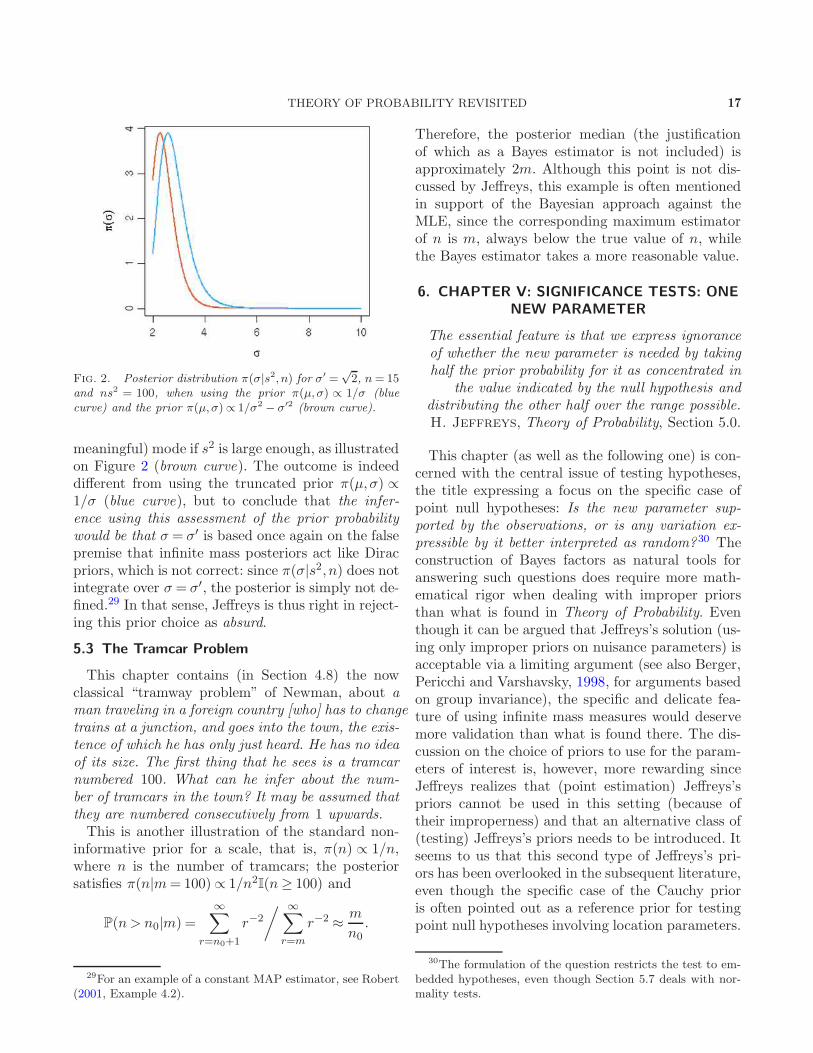
Fig. 2. Posterior distribution π(σ|s2, n) for σ′ =√2, n= 15
and ns2 = 100, when using the prior π(µ,σ) ∝ 1/σ (bluecurve) and the prior π(µ,σ)∝ 1/σ2 − σ′2 (brown curve).
meaningful) mode if s2 is large enough, as illustratedon Figure 2 (brown curve). The outcome is indeeddifferent from using the truncated prior π(µ,σ) ∝1/σ (blue curve), but to conclude that the infer-ence using this assessment of the prior probabilitywould be that σ = σ′ is based once again on the falsepremise that infinite mass posteriors act like Diracpriors, which is not correct: since π(σ|s2, n) does notintegrate over σ = σ′, the posterior is simply not de-fined.29 In that sense, Jeffreys is thus right in reject-ing this prior choice as absurd.
5.3 The Tramcar Problem
This chapter contains (in Section 4.8) the nowclassical “tramway problem” of Newman, about aman traveling in a foreign country [who] has to changetrains at a junction, and goes into the town, the exis-tence of which he has only just heard. He has no ideaof its size. The first thing that he sees is a tramcarnumbered 100. What can he infer about the num-ber of tramcars in the town? It may be assumed thatthey are numbered consecutively from 1 upwards.This is another illustration of the standard non-
informative prior for a scale, that is, π(n) ∝ 1/n,where n is the number of tramcars; the posteriorsatisfies π(n|m= 100)∝ 1/n2I(n≥ 100) and
P(n> n0|m) =∞∑
r=n0+1
r−2
/ ∞∑
r=m
r−2 ≈ m
n0.
29For an example of a constant MAP estimator, see Robert(2001, Example 4.2).
Therefore, the posterior median (the justificationof which as a Bayes estimator is not included) isapproximately 2m. Although this point is not dis-cussed by Jeffreys, this example is often mentionedin support of the Bayesian approach against theMLE, since the corresponding maximum estimatorof n is m, always below the true value of n, whilethe Bayes estimator takes a more reasonable value.
6. CHAPTER V: SIGNIFICANCE TESTS: ONE
NEW PARAMETER
The essential feature is that we express ignoranceof whether the new parameter is needed by takinghalf the prior probability for it as concentrated in
the value indicated by the null hypothesis anddistributing the other half over the range possible.H. Jeffreys, Theory of Probability, Section 5.0.
This chapter (as well as the following one) is con-cerned with the central issue of testing hypotheses,the title expressing a focus on the specific case ofpoint null hypotheses: Is the new parameter sup-ported by the observations, or is any variation ex-pressible by it better interpreted as random?30 Theconstruction of Bayes factors as natural tools foranswering such questions does require more math-ematical rigor when dealing with improper priorsthan what is found in Theory of Probability. Eventhough it can be argued that Jeffreys’s solution (us-ing only improper priors on nuisance parameters) isacceptable via a limiting argument (see also Berger,Pericchi and Varshavsky, 1998, for arguments basedon group invariance), the specific and delicate fea-ture of using infinite mass measures would deservemore validation than what is found there. The dis-cussion on the choice of priors to use for the param-eters of interest is, however, more rewarding sinceJeffreys realizes that (point estimation) Jeffreys’spriors cannot be used in this setting (because oftheir improperness) and that an alternative class of(testing) Jeffreys’s priors needs to be introduced. Itseems to us that this second type of Jeffreys’s pri-ors has been overlooked in the subsequent literature,even though the specific case of the Cauchy prioris often pointed out as a reference prior for testingpoint null hypotheses involving location parameters.
30The formulation of the question restricts the test to em-bedded hypotheses, even though Section 5.7 deals with nor-mality tests.
18 C. P. ROBERT, N. CHOPIN AND J. ROUSSEAU
6.1 Model Choice Formalism
Jeffreys starts by analyzing the question,
In what circumstances do observations sup-port a change of the form of the law it-self?,
from a model-choice perspective, by assigningprior probabilities to the models Mi that are incompetition, π(Mi) (i = 1,2, . . .). He further con-strains those probabilities to be terms of a conver-gent series.31 When checking back in Chapter I (Sec-tion 1.62), it appears that this condition is due to theconstraint that the probabilities can be normalizedto 1, which sounds like an unnecessary condition ifdealing with improper priors at the same time.32
The consequence of this constraint is that π(Mi)must decrease like 2−i or i−2 and it thus (a) pre-vents the use of equal probabilities advocated beforeand (b) imposes an ordering of models.Obviously, the use of the Bayes factor eliminates
the impact of this choice of prior probabilities, asit does for the decomposition of an alternative hy-pothesis H1 into a series of mutually irrelevant alter-native hypotheses. The fact that m alternatives aretested at once induces a Bonferroni effect, though,that is not (correctly) taken into account at the be-ginning of Section 5.04 (even if Jeffreys notes thatthe Bayes factor is then multiplied by 0.7m). Thefollowing discussion borders more on “ranking andselection” than on testing per se, although the useof Bayes factors with correction factor m or m2 isthe proposed solution. It is only at the end of Sec-tion 5.04 that the Bonferroni effect of repeated test-ing is properly recognized, if not correctly solvedfrom a Bayesian point of view.If the hypothesis to be tested is H0 : θ = 0, against
the alternative H1 that is the aggregate of other pos-sible values [of θ], Jeffreys initiates one of the majoradvances of Theory of Probability by rewriting theprior distribution as a mixture of a point mass inθ = 0 and of a generic density π on the range of θ,
π(θ) = 12I0(θ) +
12π(θ).
31The perspective of an infinite sequence of models undercomparison is not pursued further in this chapter.
32In Jeffreys (1931), Jeffreys puts forward a similar argu-ment that it is impossible to construct a theory of quantitativeinference on the hypothesis that all general laws have the sameprior probability (Section 4.3, page 43). See Earman (1992) fora deeper discussion of this point.
This is indeed a stepping stone for Bayesian Statis-tics in that it explicitly recognizes the need to sep-arate the null hypothesis from the alternative hy-pothesis within the prior, lest the null hypothesisis not properly weighted once it is accepted. Theoverall principle is illustrated for a normal setting,x ∼ N (θ,σ2) (with known σ2), so that the Bayesfactor is
K =π(H0|x)π(H1|x)
/π(H0)
π(H1)
=exp{−x2/2σ2}
∫
f(θ) exp{−(x− θ)2/2σ2}dθ .
The numerical calibration of the Bayes factor is notdirectly addressed in the main text, except via aqualitative divergence from the neutral K = 1. Ap-pendix B provides a grading of the Bayes factor, asfollows:
• Grade 0. K > 1. Null hypothesis supported.• Grade 1. 1 > K > 10−1/2. Evidence against H0,
but not worth more than a bare mention.• Grade 2. 10−1/2 >K > 10−1. Evidence against H0
substantial.• Grade 3. 10−1 >K > 10−3/2. Evidence against H0
strong.• Grade 4. 10−3/2 >K > 10−2. Evidence against H0
very strong.• Grade 5. 10−2 >K >. Evidence against H0 deci-
sive.
The comparison with the χ2 and t statistics in thisappendix shows that a given value of K leads to anincreasing (in n) value of those statistics, in agree-ment with Lindley’s paradox (see Section 6.3 below).If there are nuisance parameters ξ in the model
(Section 5.01), Jeffreys suggests using the same prioron ξ under both alternatives, π0(ξ), resulting in thegeneral Bayes factor
K =
∫
π0(ξ)f(x|ξ,0)dξ/
∫
π0(ξ)π1(θ|ξ)f(x|ξ, θ)dξ dθ,
where π1(θ|ξ) is a conditional density. Note that Jef-freys uses a normal model with Laplace’s approxi-mation to end up with the approximation
K ≈ 1
π1(θ|ξ)
√
ngθθ2π
exp
{
−1
2ngθθθ
2
}
,
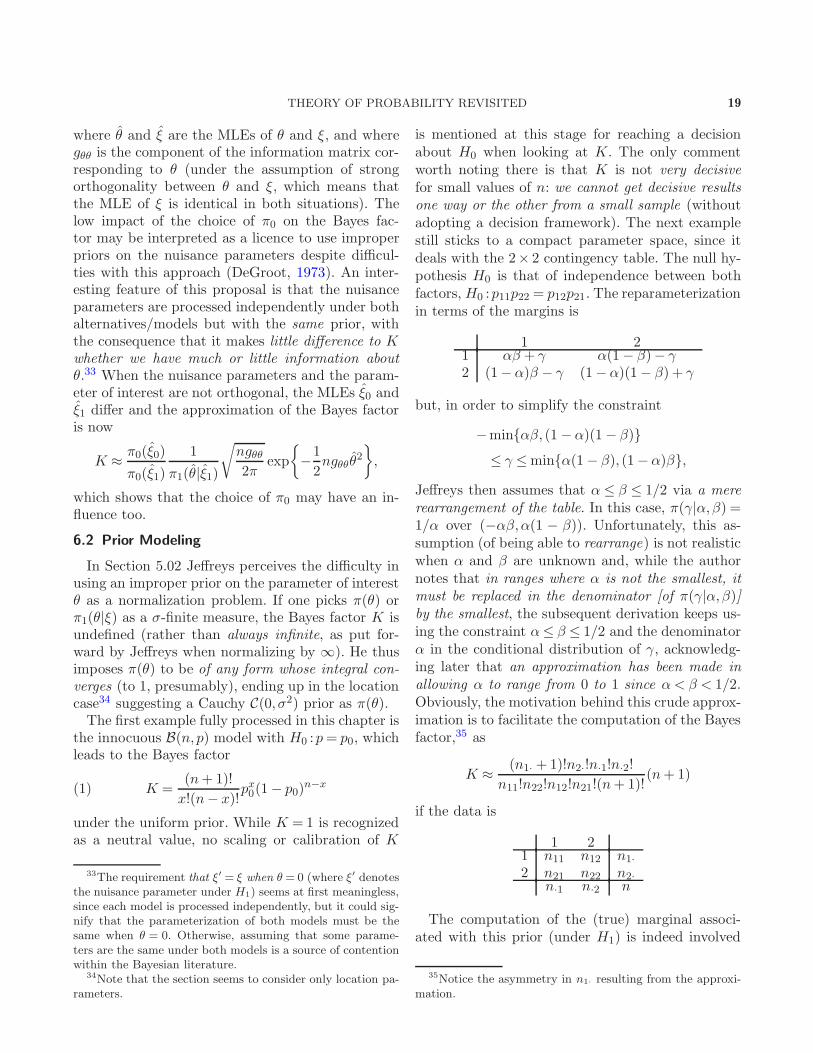
THEORY OF PROBABILITY REVISITED 19
where θ and ξ are the MLEs of θ and ξ, and wheregθθ is the component of the information matrix cor-responding to θ (under the assumption of strongorthogonality between θ and ξ, which means thatthe MLE of ξ is identical in both situations). Thelow impact of the choice of π0 on the Bayes fac-tor may be interpreted as a licence to use improperpriors on the nuisance parameters despite difficul-ties with this approach (DeGroot, 1973). An inter-esting feature of this proposal is that the nuisanceparameters are processed independently under bothalternatives/models but with the same prior, withthe consequence that it makes little difference to Kwhether we have much or little information aboutθ.33 When the nuisance parameters and the param-eter of interest are not orthogonal, the MLEs ξ0 andξ1 differ and the approximation of the Bayes factoris now
K ≈ π0(ξ0)
π0(ξ1)
1
π1(θ|ξ1)
√
ngθθ2π
exp
{
−1
2ngθθθ
2
}
,
which shows that the choice of π0 may have an in-fluence too.
6.2 Prior Modeling
In Section 5.02 Jeffreys perceives the difficulty inusing an improper prior on the parameter of interestθ as a normalization problem. If one picks π(θ) orπ1(θ|ξ) as a σ-finite measure, the Bayes factor K isundefined (rather than always infinite, as put for-ward by Jeffreys when normalizing by ∞). He thusimposes π(θ) to be of any form whose integral con-verges (to 1, presumably), ending up in the locationcase34 suggesting a Cauchy C(0, σ2) prior as π(θ).The first example fully processed in this chapter is
the innocuous B(n,p) model with H0 :p= p0, whichleads to the Bayes factor
K =(n+ 1)!
x!(n− x)!px0(1− p0)
n−x(1)
under the uniform prior. While K = 1 is recognizedas a neutral value, no scaling or calibration of K
33The requirement that ξ′ = ξ when θ = 0 (where ξ′ denotesthe nuisance parameter under H1) seems at first meaningless,since each model is processed independently, but it could sig-nify that the parameterization of both models must be thesame when θ = 0. Otherwise, assuming that some parame-ters are the same under both models is a source of contentionwithin the Bayesian literature.
34Note that the section seems to consider only location pa-rameters.
is mentioned at this stage for reaching a decisionabout H0 when looking at K. The only commentworth noting there is that K is not very decisivefor small values of n: we cannot get decisive resultsone way or the other from a small sample (withoutadopting a decision framework). The next examplestill sticks to a compact parameter space, since itdeals with the 2× 2 contingency table. The null hy-pothesis H0 is that of independence between bothfactors, H0 :p11p22 = p12p21. The reparameterizationin terms of the margins is
1 21 αβ + γ α(1− β)− γ2 (1−α)β − γ (1−α)(1− β) + γ
but, in order to simplify the constraint
−min{αβ, (1−α)(1− β)}≤ γ ≤min{α(1− β), (1−α)β},
Jeffreys then assumes that α ≤ β ≤ 1/2 via a mererearrangement of the table. In this case, π(γ|α,β) =1/α over (−αβ,α(1 − β)). Unfortunately, this as-sumption (of being able to rearrange) is not realisticwhen α and β are unknown and, while the authornotes that in ranges where α is not the smallest, itmust be replaced in the denominator [of π(γ|α,β)]by the smallest, the subsequent derivation keeps us-ing the constraint α≤ β ≤ 1/2 and the denominatorα in the conditional distribution of γ, acknowledg-ing later that an approximation has been made inallowing α to range from 0 to 1 since α < β < 1/2.Obviously, the motivation behind this crude approx-imation is to facilitate the computation of the Bayesfactor,35 as
K ≈ (n1· +1)!n2·!n·1!n·2!
n11!n22!n12!n21!(n+ 1)!(n+ 1)
if the data is
1 21 n11 n12 n1·2 n21 n22 n2·
n·1 n·2 n
The computation of the (true) marginal associ-ated with this prior (under H1) is indeed involved
35Notice the asymmetry in n1· resulting from the approxi-mation.
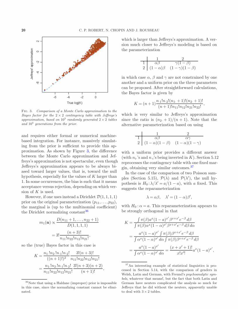
20 C. P. ROBERT, N. CHOPIN AND J. ROUSSEAU
Fig. 3. Comparison of a Monte Carlo approximation to theBayes factor for the 2 × 2 contingency table with Jeffreys’sapproximation, based on 103 randomly generated 2× 2 tablesand 104 generations from the prior.
and requires either formal or numerical machine-based integration. For instance, massively simulat-ing from the prior is sufficient to provide this ap-proximation. As shown by Figure 3, the differencebetween the Monte Carlo approximation and Jef-freys’s approximation is not spectacular, even thoughJeffreys’s approximation appears to be always bi-ased toward larger values, that is, toward the nullhypothesis, especially for the values of K larger than1. In some occurrences, the bias is such that it meansacceptance versus rejection, depending on which ver-sion of K is used.However, if one uses instead a Dirichlet D(1,1,1,1)
prior on the original parameterization (p11, . . . , p22),the marginal is (up to the multinomial coefficient)the Dirichlet normalizing constant36
m1(n)∝D(n11 +1, . . . , n22 +1)
D(1,1,1,1)
= 3!(n+3)!
n11!n22!n12!n21!,
so the (true) Bayes factor in this case is
K =n1·!n2·!n·1!n·2!
((n+1)!)23!(n+3)!
n11!n22!n12!n21!
=n1·!n2·!n·1!n·2!
n11!n22!n12!n21!
3!(n+3)(n+2)
(n+ 1)!,
36Note that using a Haldane (improper) prior is impossiblein this case, since the normalizing constant cannot be elimi-nated.
which is larger than Jeffreys’s approximation. A ver-sion much closer to Jeffreys’s modeling is based onthe parameterization
1 21 αβ γ(1− β)2 (1− α)β (1− γ)(1− β)
in which case α, β and γ are not constrained by oneanother and a uniform prior on the three parameterscan be proposed. After straightforward calculations,the Bayes factor is given by
K = (n+1)n·1!n·2!(n1· + 1)!(n2· + 1)!
(n+ 1)!n11!n12!n21!n22!,
which is very similar to Jeffreys’s approximationsince the ratio is (n2· + 1)/(n + 1). Note that thealternative parameterization based on using
1 21 αβ αγ2 (1−α)(1− β) (1−α)(1− γ)
with a uniform prior provides a different answer(with ni·’s and n·i’s being inverted inK). Section 5.12reprocesses the contingency table with one fixed mar-gin, obtaining very similar outcomes.37
In the case of the comparison of two Poisson sam-ples (Section 5.15), P(λ) and P(λ′), the null hy-pothesis is H0 :λ/λ
′ = a/(1− a), with a fixed. Thissuggests the reparameterization
λ= αβ, λ′ = (1−α)β′,
with H0 : α= a. This reparameterization appears tobe strongly orthogonal in that
K =
∫
π(β)ax(1− a)x′βx+x′
e−β dβ∫
π(β)αx(1− α)x′βx+x′e−β dβ dα
=ax(1− a)x
′ ∫
π(β)βx+x′e−β dβ
∫
αx(1− α)x′ dα∫
π(β)βx+x′e−β dβ
=ax(1− a)x
′
∫
αx(1− α)x′ dα=
(x+ x′ +1)!
x!x′!ax(1− a)x
′
,
37An interesting example of statistical linguistics is pro-cessed in Section 5.14, with the comparison of genders inWelsh, Latin and German, with Freund’s psychoanalytic sym-bols, whatever that means!, but the fact that both Latin andGerman have neuters complicated the analysis so much forJeffreys that he did without the neuters, apparently unableto deal with 3× 2 tables.
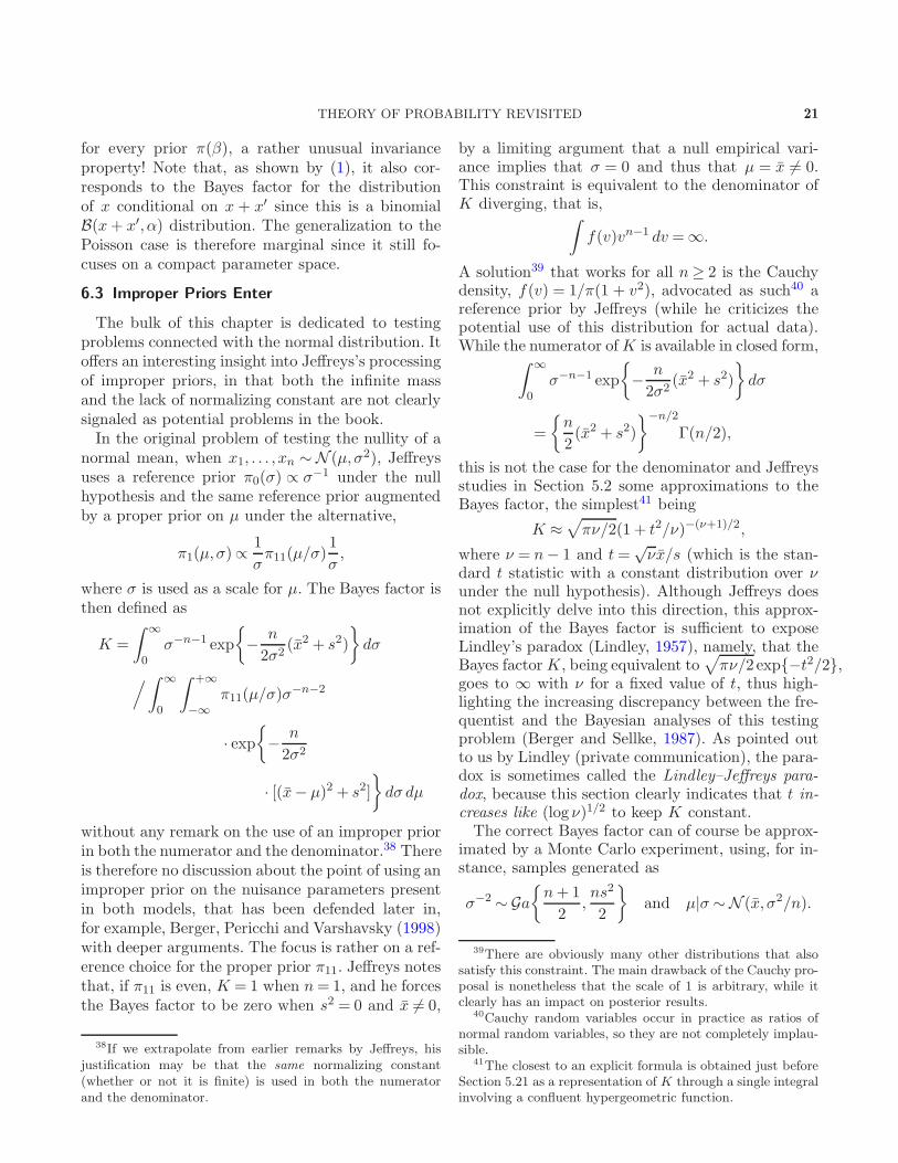
THEORY OF PROBABILITY REVISITED 21
for every prior π(β), a rather unusual invarianceproperty! Note that, as shown by (1), it also cor-responds to the Bayes factor for the distributionof x conditional on x + x′ since this is a binomialB(x+ x′, α) distribution. The generalization to thePoisson case is therefore marginal since it still fo-cuses on a compact parameter space.
6.3 Improper Priors Enter
The bulk of this chapter is dedicated to testingproblems connected with the normal distribution. Itoffers an interesting insight into Jeffreys’s processingof improper priors, in that both the infinite massand the lack of normalizing constant are not clearlysignaled as potential problems in the book.In the original problem of testing the nullity of a
normal mean, when x1, . . . , xn ∼ N (µ,σ2), Jeffreysuses a reference prior π0(σ) ∝ σ−1 under the nullhypothesis and the same reference prior augmentedby a proper prior on µ under the alternative,
π1(µ,σ)∝1
σπ11(µ/σ)
1
σ,
where σ is used as a scale for µ. The Bayes factor isthen defined as
K =
∫ ∞
0σ−n−1 exp
{
− n
2σ2(x2 + s2)
}
dσ
/
∫ ∞
0
∫ +∞
−∞π11(µ/σ)σ
−n−2
· exp{
− n
2σ2
· [(x− µ)2 + s2]
}
dσ dµ
without any remark on the use of an improper priorin both the numerator and the denominator.38 Thereis therefore no discussion about the point of using animproper prior on the nuisance parameters presentin both models, that has been defended later in,for example, Berger, Pericchi and Varshavsky (1998)with deeper arguments. The focus is rather on a ref-erence choice for the proper prior π11. Jeffreys notesthat, if π11 is even, K = 1 when n= 1, and he forcesthe Bayes factor to be zero when s2 = 0 and x 6= 0,
38If we extrapolate from earlier remarks by Jeffreys, hisjustification may be that the same normalizing constant(whether or not it is finite) is used in both the numeratorand the denominator.
by a limiting argument that a null empirical vari-ance implies that σ = 0 and thus that µ = x 6= 0.This constraint is equivalent to the denominator ofK diverging, that is,
∫
f(v)vn−1 dv =∞.
A solution39 that works for all n≥ 2 is the Cauchydensity, f(v) = 1/π(1 + v2), advocated as such40 areference prior by Jeffreys (while he criticizes thepotential use of this distribution for actual data).While the numerator ofK is available in closed form,
∫ ∞
0σ−n−1 exp
{
− n
2σ2(x2 + s2)
}
dσ
=
{
n
2(x2 + s2)
}−n/2
Γ(n/2),
this is not the case for the denominator and Jeffreysstudies in Section 5.2 some approximations to theBayes factor, the simplest41 being
K ≈√
πν/2(1 + t2/ν)−(ν+1)/2,
where ν = n− 1 and t=√νx/s (which is the stan-
dard t statistic with a constant distribution over νunder the null hypothesis). Although Jeffreys doesnot explicitly delve into this direction, this approx-imation of the Bayes factor is sufficient to exposeLindley’s paradox (Lindley, 1957), namely, that theBayes factorK, being equivalent to
√
πν/2 exp{−t2/2},goes to ∞ with ν for a fixed value of t, thus high-lighting the increasing discrepancy between the fre-quentist and the Bayesian analyses of this testingproblem (Berger and Sellke, 1987). As pointed outto us by Lindley (private communication), the para-dox is sometimes called the Lindley–Jeffreys para-dox, because this section clearly indicates that t in-creases like (log ν)1/2 to keep K constant.The correct Bayes factor can of course be approx-
imated by a Monte Carlo experiment, using, for in-stance, samples generated as
σ−2 ∼ Ga{
n+1
2,ns2
2
}
and µ|σ ∼N (x, σ2/n).
39There are obviously many other distributions that alsosatisfy this constraint. The main drawback of the Cauchy pro-posal is nonetheless that the scale of 1 is arbitrary, while itclearly has an impact on posterior results.
40Cauchy random variables occur in practice as ratios ofnormal random variables, so they are not completely implau-sible.
41The closest to an explicit formula is obtained just beforeSection 5.21 as a representation of K through a single integralinvolving a confluent hypergeometric function.
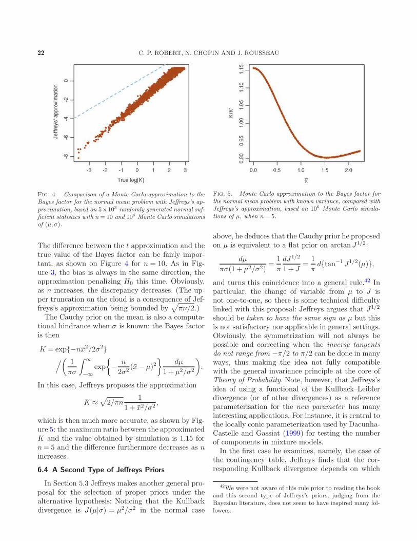
22 C. P. ROBERT, N. CHOPIN AND J. ROUSSEAU
Fig. 4. Comparison of a Monte Carlo approximation to theBayes factor for the normal mean problem with Jeffreys’s ap-proximation, based on 5×10³ randomly generated normal suf-ficient statistics with n= 10 and 104 Monte Carlo simulationsof (µ,σ).
The difference between the t approximation and thetrue value of the Bayes factor can be fairly impor-tant, as shown on Figure 4 for n = 10. As in Fig-ure 3, the bias is always in the same direction, theapproximation penalizing H0 this time. Obviously,as n increases, the discrepancy decreases. (The up-per truncation on the cloud is a consequence of Jef-freys’s approximation being bounded by
√
πν/2.)The Cauchy prior on the mean is also a computa-
tional hindrance when σ is known: the Bayes factoris then
K = exp{−nx2/2σ2}/
(
1
πσ
∫ ∞
−∞exp
{
− n
2σ2(x− µ)2
}
dµ
1 + µ2/σ2
)
.
In this case, Jeffreys proposes the approximation
K ≈√
2/πn1
1 + x2/σ2,
which is then much more accurate, as shown by Fig-ure 5: the maximum ratio between the approximatedK and the value obtained by simulation is 1.15 forn= 5 and the difference furthermore decreases as nincreases.
6.4 A Second Type of Jeffreys Priors
In Section 5.3 Jeffreys makes another general pro-posal for the selection of proper priors under thealternative hypothesis: Noticing that the Kullbackdivergence is J(µ|σ) = µ2/σ2 in the normal case
Fig. 5. Monte Carlo approximation to the Bayes factor forthe normal mean problem with known variance, compared withJeffreys’s approximation, based on 106 Monte Carlo simula-tions of µ, when n= 5.
above, he deduces that the Cauchy prior he proposedon µ is equivalent to a flat prior on arctanJ1/2:
dµ
πσ(1 + µ2/σ2)=
1
π
dJ1/2
1 + J=
1
πd{tan−1 J1/2(µ)},
and turns this coincidence into a general rule.42 Inparticular, the change of variable from µ to J isnot one-to-one, so there is some technical difficultylinked with this proposal: Jeffreys argues that J1/2
should be taken to have the same sign as µ but thisis not satisfactory nor applicable in general settings.Obviously, the symmetrization will not always bepossible and correcting when the inverse tangentsdo not range from −π/2 to π/2 can be done in manyways, thus making the idea not fully compatiblewith the general invariance principle at the core ofTheory of Probability. Note, however, that Jeffreys’sidea of using a functional of the Kullback–Leiblerdivergence (or of other divergences) as a referenceparameterisation for the new parameter has manyinteresting applications. For instance, it is central tothe locally conic parameterization used by Dacunha-Castelle and Gassiat (1999) for testing the numberof components in mixture models.In the first case he examines, namely, the case of
the contingency table, Jeffreys finds that the cor-responding Kullback divergence depends on which
42We were not aware of this rule prior to reading the bookand this second type of Jeffreys’s priors, judging from theBayesian literature, does not seem to have inspired many fol-lowers.
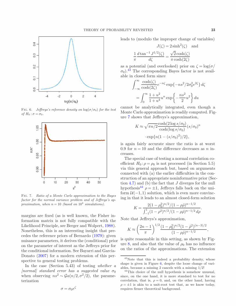
THEORY OF PROBABILITY REVISITED 23
Fig. 6. Jeffreys’s reference density on log(σ/σ0) for the testof H0 : σ = σ0.
Fig. 7. Ratio of a Monte Carlo approximation to the Bayesfactor for the normal variance problem and of Jeffreys’s ap-proximation, when n= 10 (based on 104 simulations).
margins are fixed (as is well known, the Fisher in-formation matrix is not fully compatible with theLikelihood Principle, see Berger and Wolpert, 1988).Nonetheless, this is an interesting insight that pre-cedes the reference priors of Bernardo (1979): givennuisance parameters, it derives the (conditional) prioron the parameter of interest as the Jeffreys prior forthe conditional information. See Bayarri and Garcia-Donato (2007) for a modern extension of this per-spective to general testing problems.In the case (Section 5.43) of testing whether a
[normal] standard error has a suggested value σ0when observing ns2 ∼ Ga(n/2, σ2/2), the parame-terization
σ = σ0eζ
leads to (modulo the improper change of variables)
J(ζ) = 2sinh2(ζ) and
1
π
d tan−1 J1/2(ζ)
dζ=
√2cosh(ζ)
π cosh(2ζ)
as a potential (and overlooked) prior on ζ = log(σ/σ0).
43 The corresponding Bayes factor is not avail-able in closed form since
∫ ∞
−∞
cosh(ζ)
cosh(2ζ)e−nζ exp{−ns2/2σ20e2ζ}dζ
=
∫ ∞
0
1 + u2
1 + u4un exp
{
−ns2
2u2
}
du
cannot be analytically integrated, even though aMonte Carlo approximation is readily computed. Fig-ure 7 shows that Jeffreys’s approximation,
K ≈√
πn/2cosh(2 log s/σ0)
cosh(log s/σ0)(s/σ0)
n
· exp{n(1− (s/σ0)2)/2},
is again fairly accurate since the ratio is at worst0.9 for n= 10 and the difference decreases as n in-creases.The special case of testing a normal correlation co-
efficient H0 :ρ= ρ0 is not processed (in Section 5.5)via this general approach but, based on argumentsconnected with (a) the earlier difficulties in the con-struction of an appropriate noninformative prior (Sec-tion 4.7) and (b) the fact that J diverges for the nullhypothesis44 ρ=±1, Jeffreys falls back on the uni-form U(−1,1) solution, which is even more convinc-ing in that it leads to an almost closed-form solution
K =2(1− ρ20)
n/2/(1− ρρ)n−1/2
∫ 1−1(1− ρ2)n/2/(1− ρρ)n−1/2 dρ
.
Note that Jeffreys’s approximation,
K ≈(
2n− 1
π
)1/2 (1− ρ20)n/2(1− ρ2)(n−3)/2
(1− ρρ)n−1/2,
is quite reasonable in this setting, as shown by Fig-ure 8, and also that the value of ρ0 has no influenceon the ratios of the approximations. The extension
43Note that this is indeed a probability density, whoseshape is given in Figure 6, despite the loose change of vari-ables, because a missing 2 cancels with a missing 1/2!
44This choice of the null hypothesis is somehow unusual,since, on the one hand, it is more standard to test for nocorrelation, that is, ρ = 0, and, on the other hand, havingρ = ±1 is akin to a unit-root test that, as we know today,requires firmer theoretical background.
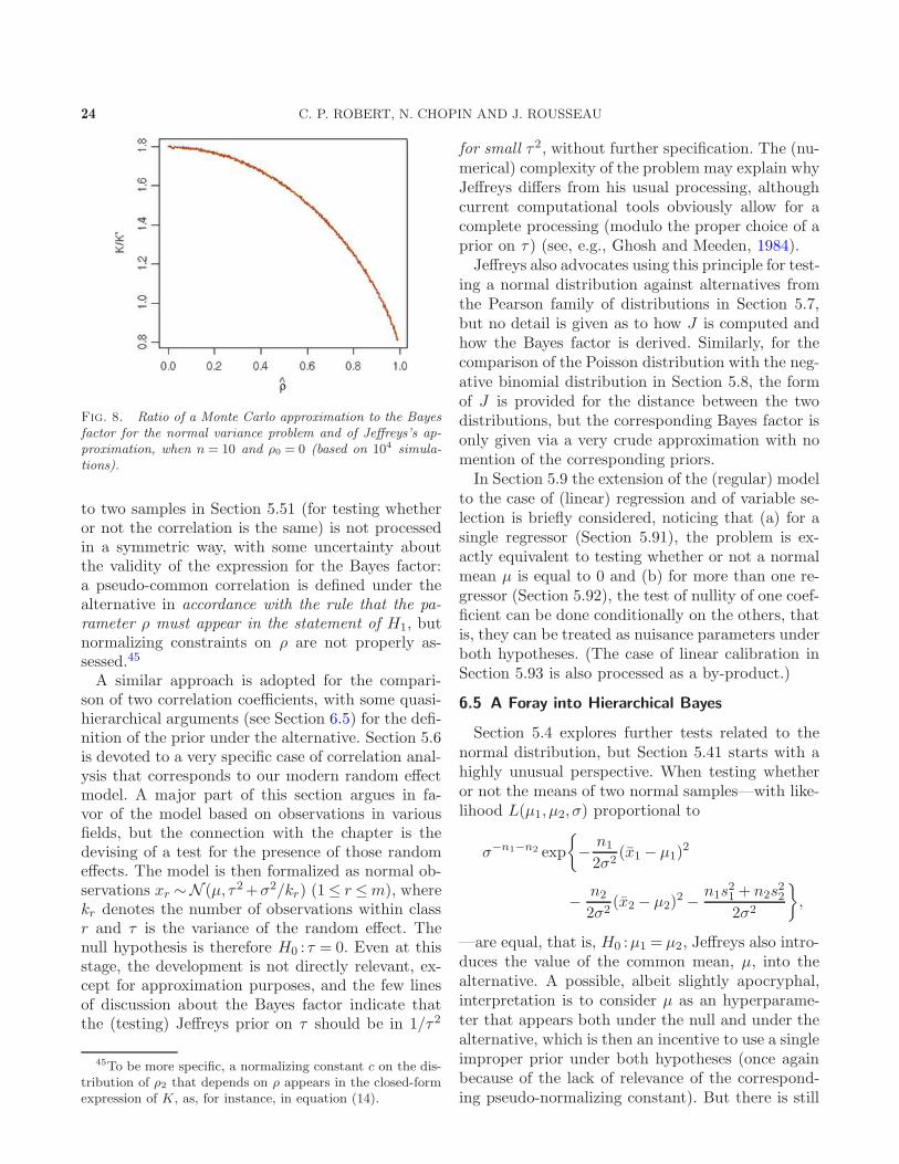
24 C. P. ROBERT, N. CHOPIN AND J. ROUSSEAU
Fig. 8. Ratio of a Monte Carlo approximation to the Bayesfactor for the normal variance problem and of Jeffreys’s ap-proximation, when n = 10 and ρ0 = 0 (based on 104 simula-tions).
to two samples in Section 5.51 (for testing whetheror not the correlation is the same) is not processedin a symmetric way, with some uncertainty aboutthe validity of the expression for the Bayes factor:a pseudo-common correlation is defined under thealternative in accordance with the rule that the pa-rameter ρ must appear in the statement of H1, butnormalizing constraints on ρ are not properly as-sessed.45
A similar approach is adopted for the compari-son of two correlation coefficients, with some quasi-hierarchical arguments (see Section 6.5) for the defi-nition of the prior under the alternative. Section 5.6is devoted to a very specific case of correlation anal-ysis that corresponds to our modern random effectmodel. A major part of this section argues in fa-vor of the model based on observations in variousfields, but the connection with the chapter is thedevising of a test for the presence of those randomeffects. The model is then formalized as normal ob-servations xr ∼N (µ, τ2+σ2/kr) (1≤ r≤m), wherekr denotes the number of observations within classr and τ is the variance of the random effect. Thenull hypothesis is therefore H0 : τ = 0. Even at thisstage, the development is not directly relevant, ex-cept for approximation purposes, and the few linesof discussion about the Bayes factor indicate thatthe (testing) Jeffreys prior on τ should be in 1/τ2
45To be more specific, a normalizing constant c on the dis-tribution of ρ2 that depends on ρ appears in the closed-formexpression of K, as, for instance, in equation (14).
for small τ2, without further specification. The (nu-merical) complexity of the problem may explain whyJeffreys differs from his usual processing, althoughcurrent computational tools obviously allow for acomplete processing (modulo the proper choice of aprior on τ ) (see, e.g., Ghosh and Meeden, 1984).Jeffreys also advocates using this principle for test-
ing a normal distribution against alternatives fromthe Pearson family of distributions in Section 5.7,but no detail is given as to how J is computed andhow the Bayes factor is derived. Similarly, for thecomparison of the Poisson distribution with the neg-ative binomial distribution in Section 5.8, the formof J is provided for the distance between the twodistributions, but the corresponding Bayes factor isonly given via a very crude approximation with nomention of the corresponding priors.In Section 5.9 the extension of the (regular) model
to the case of (linear) regression and of variable se-lection is briefly considered, noticing that (a) for asingle regressor (Section 5.91), the problem is ex-actly equivalent to testing whether or not a normalmean µ is equal to 0 and (b) for more than one re-gressor (Section 5.92), the test of nullity of one coef-ficient can be done conditionally on the others, thatis, they can be treated as nuisance parameters underboth hypotheses. (The case of linear calibration inSection 5.93 is also processed as a by-product.)
6.5 A Foray into Hierarchical Bayes
Section 5.4 explores further tests related to thenormal distribution, but Section 5.41 starts with ahighly unusual perspective. When testing whetheror not the means of two normal samples—with like-lihood L(µ1, µ2, σ) proportional to
σ−n1−n2 exp
{
− n12σ2
(x1 − µ1)2
− n22σ2
(x2 − µ2)2 − n1s
21 + n2s
22
2σ2
}
,
—are equal, that is, H0 :µ1 = µ2, Jeffreys also intro-duces the value of the common mean, µ, into thealternative. A possible, albeit slightly apocryphal,interpretation is to consider µ as an hyperparame-ter that appears both under the null and under thealternative, which is then an incentive to use a singleimproper prior under both hypotheses (once againbecause of the lack of relevance of the correspond-ing pseudo-normalizing constant). But there is still
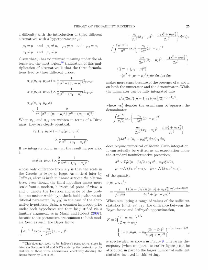
THEORY OF PROBABILITY REVISITED 25
a difficulty with the introduction of three differentalternatives with a hyperparameter µ:
µ1 = µ and µ2 6= µ, µ1 6= µ and µ2 = µ,
µ1 6= µ and µ2 6= µ.
Given that µ has no intrinsic meaning under the al-ternative, the most logical46 translation of this mul-tiplication of alternatives is that the three formula-tions lead to three different priors,
π11(µ,µ1, µ2, σ)∝1
π
1
σ2 + (µ2 − µ)2Iµ1=µ,
π12(µ,µ1, µ2, σ)∝1
π
1
σ2 + (µ1 − µ)2Iµ2=µ,
π13(µ,µ1, µ2, σ)
∝ 1
π2σ
{σ2 + (µ1 − µ)2}{σ2 + (µ2 − µ)2} .
When π11 and π12 are written in terms of a Diracmass, they are clearly identical,
π11(µ1, µ2, σ) = π12(µ1, µ2, σ)
∝ 1
π
1
σ2 + (µ1 − µ2)2.
If we integrate out µ in π13, the resulting posterioris
π13(µ1, µ2, σ)∝2
π
1
4σ2 + (µ1 − µ2)2,
whose only difference from π11 is that the scale inthe Cauchy is twice as large. As noticed later byJeffreys, there is little to choose between the alterna-tives, even though the third modeling makes moresense from a modern, hierarchical point of view: µand σ denote the location and scale of the prob-lem, no matter which hypothesis holds, with an ad-ditional parameter (µ1, µ2) in the case of the alter-native hypothesis. Using a common improper priorunder both hypotheses can then be justified via alimiting argument, as in Marin and Robert (2007),because those parameters are common to both mod-els. Seen as such, the Bayes factor∫
σ−n−1 exp
{
− n12σ2
(x1 − µ)2
46This does not seem to be Jeffreys’s perspective, since helater (in Sections 5.46 and 5.47) adds up the posterior prob-abilities of those three alternatives, effectively dividing theBayes factor by 3 or such.
− n22σ2
(x2 − µ)2 − n1s21 + n2s
22
2σ2
}
dσ dµ
/
∫
σ−n+1
π2exp
{
− n12σ2
(x1 − µ1)2
− n22σ2
(x2 − µ2)2 − n1s
21 + n2s
22
2σ2
}
/({σ2 + (µ1 − µ)2}· {σ2 + (µ2 − µ)2})dσ dµdµ1 dµ2
makes more sense because of the presence of σ and µon both the numerator and the denominator. Whilethe numerator can be fully integrated into
√
π/2nΓ{(n− 1)/2}(ns20/2)−(n−1)/2,
where ns20 denotes the usual sum of squares, thedenominator
∫
σ−n
π/2exp
{
− n12σ2
(x1 − µ1)2
− n22σ2
(x2 − µ2)2 − n1s
21 + n2s
22
2σ2
}
/(4σ2 + (µ1 − µ2)2)dσ dµ1 dµ2
does require numerical or Monte Carlo integration.It can actually be written as an expectation underthe standard noninformative posteriors,
σ2 ∼ IG((n− 3)/2, (n1s21 + n2s
22)/2),
µ1 ∼N (x1, σ2/n1), µ2 ∼N (x2, σ
2/n2),
of the quantity
h(µ1, µ2, σ2)
=2√n1n2
Γ((n− 3)/2){(n1s21 + n2s22)/2}−(n−3)/2
4σ2 + (µ1 − µ2)2.
When simulating a range of values of the sufficientstatistics (ni, xi, si)i=1,2, the difference between theBayes factor and Jeffreys’s approximation,
K ≈ 2
(
π
2
n1n2n1 + n2
)1/2
·{
1 + n1n2n1 + n2(x1 − x2)
2
n1s21 + n2s2
}−(n1+n2−1)/2
,
is spectacular, as shown in Figure 9. The larger dis-crepancy (when compared to earlier figures) can beattributed in part to the larger number of sufficientstatistics involved in this setting.
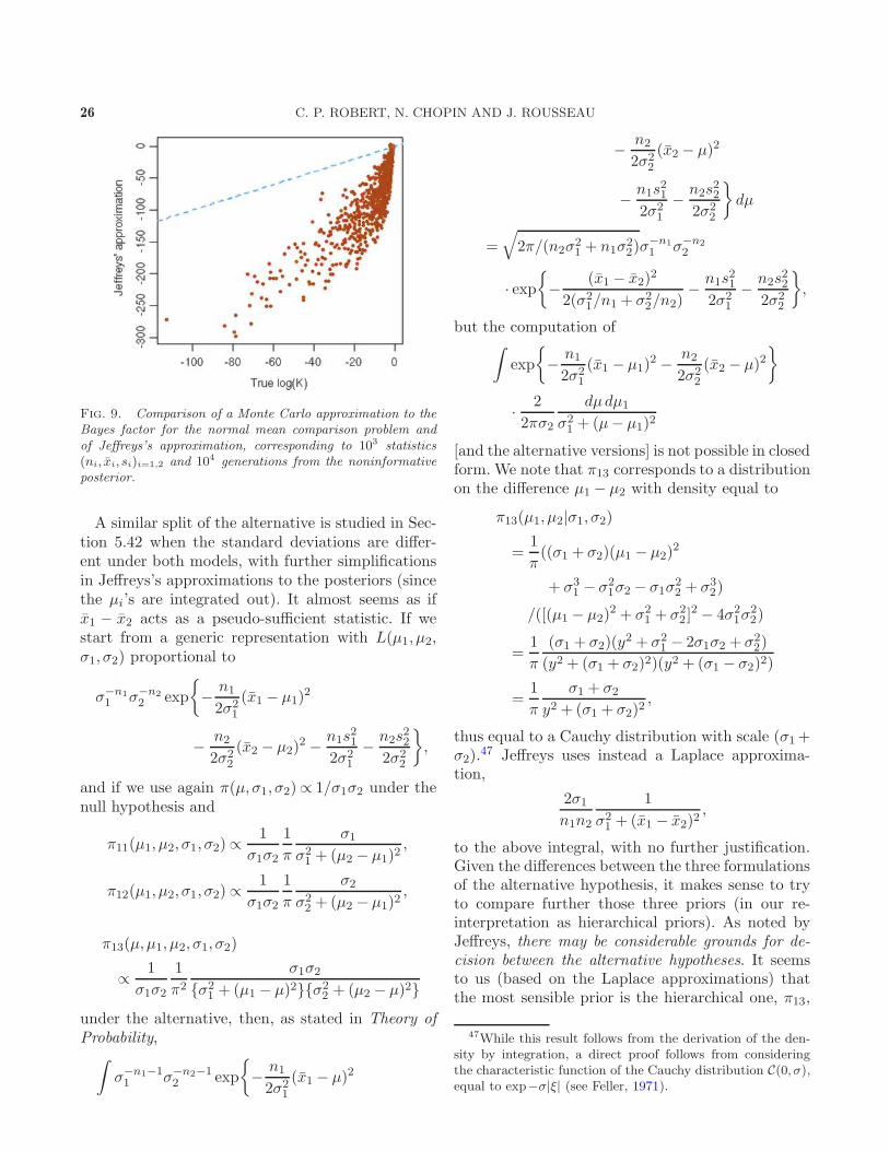
26 C. P. ROBERT, N. CHOPIN AND J. ROUSSEAU
Fig. 9. Comparison of a Monte Carlo approximation to theBayes factor for the normal mean comparison problem andof Jeffreys’s approximation, corresponding to 103 statistics(ni, xi, si)i=1,2 and 104 generations from the noninformativeposterior.
A similar split of the alternative is studied in Sec-tion 5.42 when the standard deviations are differ-ent under both models, with further simplificationsin Jeffreys’s approximations to the posteriors (sincethe µi’s are integrated out). It almost seems as ifx1 − x2 acts as a pseudo-sufficient statistic. If westart from a generic representation with L(µ1, µ2,σ1, σ2) proportional to
σ−n11 σ−n2
2 exp
{
− n12σ21
(x1 − µ1)2
− n22σ22
(x2 − µ2)2 − n1s
21
2σ21− n2s
22
2σ22
}
,
and if we use again π(µ,σ1, σ2)∝ 1/σ1σ2 under thenull hypothesis and
π11(µ1, µ2, σ1, σ2)∝1
σ1σ2
1
π
σ1σ21 + (µ2 − µ1)2
,
π12(µ1, µ2, σ1, σ2)∝1
σ1σ2
1
π
σ2σ22 + (µ2 − µ1)2
,
π13(µ,µ1, µ2, σ1, σ2)
∝ 1
σ1σ2
1
π2σ1σ2
{σ21 + (µ1 − µ)2}{σ22 + (µ2 − µ)2}under the alternative, then, as stated in Theory ofProbability,
∫
σ−n1−11 σ−n2−1
2 exp
{
− n12σ21
(x1 − µ)2
− n22σ22
(x2 − µ)2
− n1s21
2σ21− n2s
22
2σ22
}
dµ
=√
2π/(n2σ21 + n1σ22)σ−n11 σ−n2
2
· exp{
− (x1 − x2)2
2(σ21/n1 + σ22/n2)− n1s
21
2σ21− n2s
22
2σ22
}
,
but the computation of∫
exp
{
− n12σ21
(x1 − µ1)2 − n2
2σ22(x2 − µ)2
}
· 2
2πσ2
dµdµ1σ21 + (µ− µ1)2
[and the alternative versions] is not possible in closedform. We note that π13 corresponds to a distributionon the difference µ1 − µ2 with density equal to
π13(µ1, µ2|σ1, σ2)
=1
π((σ1 + σ2)(µ1 − µ2)
2
+ σ31 − σ21σ2 − σ1σ22 + σ32)
/([(µ1 − µ2)2 + σ21 + σ22 ]
2 − 4σ21σ22)
=1
π
(σ1 + σ2)(y2 + σ21 − 2σ1σ2 + σ22)
(y2 + (σ1 + σ2)2)(y2 + (σ1 − σ2)2)
=1
π
σ1 + σ2y2 + (σ1 + σ2)2
,
thus equal to a Cauchy distribution with scale (σ1+σ2).
47 Jeffreys uses instead a Laplace approxima-tion,
2σ1n1n2
1
σ21 + (x1 − x2)2,
to the above integral, with no further justification.Given the differences between the three formulationsof the alternative hypothesis, it makes sense to tryto compare further those three priors (in our re-interpretation as hierarchical priors). As noted byJeffreys, there may be considerable grounds for de-cision between the alternative hypotheses. It seemsto us (based on the Laplace approximations) thatthe most sensible prior is the hierarchical one, π13,
47While this result follows from the derivation of the den-sity by integration, a direct proof follows from consideringthe characteristic function of the Cauchy distribution C(0, σ),equal to exp−σ|ξ| (see Feller, 1971).
THEORY OF PROBABILITY REVISITED 27
in that the scale depends on both variances ratherthan only one.An extension of the test on a (normal) standard
deviation is considered in Section 5.44 for the agree-ment of two estimated standard errors. Once again,the most straightforward interpretation of Jeffreys’sderivation is to see it as a hierarchical modeling,with a reference prior π(σ) = 1/σ on a global scale,σ1 say, and the corresponding (testing) Jeffreys prioron the ratio σ1/σ2 = exp ζ . The Bayes factor (in fa-vor of the null hypothesis) is then given by
K =
√2
π/
∫ ∞
−∞
cosh(ζ)
cosh(2ζ)e−n1ζ
(
n1e2(z−ζ) + n2
n2e2z + n2
)−n/2
dζ,
if z denotes log s1/s2 = log σ1/σ2.
6.6 P -what?!
Section 5.6 embarks upon a historically interest-ing discussion on the warnings given by too good ap-value: if, for instance, a χ2 test leads to a value ofthe χ2 statistic that is very small, this means (al-most certain) incompatibility with the χ2 assump-tion just as well as too large a value. (Jeffreys re-calls the example of the data set of Mendel that wasmodified by hand to agree with the Mendelian lawof inheritance, leading to too small a χ2 value.) Thiscan be seen as an indirect criticism of the standardtests (see also Section 8 below).
7. CHAPTER VI: SIGNIFICANCE TESTS:
VARIOUS COMPLICATIONS
The best way of testing differences from asystematic rule is always to arrange our work so as
to ask and answer one question at a time.H. Jeffreys, Theory of Probability, Section 6.1.
This chapter appears as a marginalia of the pre-vious one in that it contains no major advance butrather a sequence of remarks, such as, for instance,an entry on time-series models (see Section 7.2 be-low). The very first paragraph of this chapter pro-duces a remarkably simple and intuitive justificationof the incompatibility between improper priors andsignificance tests: the mere fact that we are seriouslyconsidering the possibility that it is zero may be as-sociated with a presumption that if it is not zero itis probably small.
Then, Section 6.0 discusses the difficulty of set-tling for an informative prior distribution that takesinto account the actual state of knowledge. By subdi-viding the sample into groups, different conclusionscan obviously be reached, but this contradicts theLikelihood Principle that the whole data set mustbe used simultaneously. Of course, this could alsobe interpreted as a precursor attempt at definingpseudo-Bayes factors (Berger and Pericchi, 1996).Otherwise, as correctly pointed out by Jeffreys, theprior probability when each subsample is consideredis not the original prior probability but the poste-rior probability left by the previous one, which isthe basic implementation of the Bayesian learningprinciple. However, even with this correction, thefinal outcome of a sequential approach is not theproper Bayesian solution, unless posteriors are alsoused within the integrals of the Bayes factor.Section 6.5 also recapitulates both Chapters V
and VI with general comments. It reiterates the warn-ing, already made earlier, that the Bayes factors ob-tained via this noninformative approach are usuallyrarely immensely in favor of H0. This somehow con-tradicts later studies, like those of Berger and Sellke(1987) and Berger, Boukai and Wang (1997), thatthe Bayes factor is generally less prone to reject thenull hypothesis. Jeffreys argues that, when an alter-native is actually used (. . .), the probability that it isfalse is always of order n−1/2, without further justi-fication. Note that this last section also includes theseeds of model averaging: when a set of alternativehypotheses (models Mr) is considered, the predic-tive should be
p(x′|x) =∑
r
pr(x′|x)π(Mr|x),
rather than conditional on the accepted hypothesis.Obviously, when K is large, [this] will give almostthe same inference as the selected model/hypothesis.
7.1 Multiple Parameters
Although it should proceed from first principles,the extension of Jeffreys’s (second) rule for selectionpriors (see Section 6.4) to several parameters is dis-cussed in Sections 6.1 and 6.2 in a spirit similar tothe reference priors of Berger and Bernardo (1992),by pointing out that, if two parameters α and β areintroduced sequentially against the null hypothesisH0 :α = β = 0, testing first that α 6= 0 then β 6= 0conditional on α does not lead to the same joint
28 C. P. ROBERT, N. CHOPIN AND J. ROUSSEAU
prior as the symmetric steps of testing first β 6= 0then α 6= 0 conditional on β. In fact,
darctanJ1/2α darctanJ
1/2β|α
6= darctanJ1/2β darctanJ
1/2α|β .
Jeffreys then suggests using instead the marginal-ized version
π(α,β) =1
π2
dJ1/2αdα
1 + Jα
dJ1/2β
dβ
1 + Jβ,
although he acknowledges that there are cases wherethe symmetry does not make sense (as, for instance,when parameters are not defined under the null, as,e.g., in a mixture setting). He then resorts to Ock-ham’s razor (Section 6.12) to rank those unidimen-sional tests by stating that there is a best order ofprocedures, although there are cases where such anordering is arbitrary or not even possible. Section 6.2considers a two-dimensional parameter (λ,µ) and,switching to polar coordinates, uses a (half-)Cauchy
prior on the radius ρ =√
λ2 + µ2 (and a uniformprior on the angle). The Bayes factor for testing thenullity of the parameter (λ,µ) is then
K =
∫
σ−2n−1 exp
{
−2ns2 + n(x2 + y2)
2σ2
}
dσ
/
∫
1
π2σ2n
· exp{−(2ns2
+ n([x− λ]2
+ [y − µ]2))/2σ2} dλdµdσ
ρ(σ2 + ρ2)
= 2n(n− 1)!{2ns2 + n(x2 + y2)}−n
/
∫
1
π2σ2n
· exp{
− n
2σ2
· [2s2 + ρ2
− 2ρρ cosφ+ ρ2]
}
dφdρdσ
ρ(σ2 + ρ2),
where ρ2 = x2+ y2 and which can only be integratedup to
1
K=
2
π
∫ ∞
0exp
(
− ns2v2
2s2 + ρ2
)
· 1F1
{
1− n,1,− nρ2v2
2(2s2 + ρ2)
}
dv
1 + v2,
1F1 denoting a confluent hypergeometric function.A similar analysis is conducted in Section 6.21 fora linear regression model associated with a pair ofharmonics (xt = α cos t+ β sin t+ εt), the only dif-ference being the inclusion of the covariate scales Aand B within the prior,
π(α,β|σ)
=
√A2 +B2
π2√2
· σ√
α2 + β2{σ2 + (A2 +B2)(α2 + β2)/2}.
7.2 Markovian Models
While the title of Section 6.3 (Partial and serialcorrelation) is slightly misleading, this section dealswith an AR(1) model,
xt+1 = ρxt + τεt.
It is not conclusive with respect to the selection ofthe prior on ρ given that Jeffreys does not considerthe null value ρ= 0 but rather ρ= ±1 which leadsto difficulties, if only because there is no stationarydistribution in that case. Since the Kullback diver-gence is given by
J(ρ, ρ′) =1+ ρρ′
(1− ρ2)(1− ρ′2)(ρ′ − ρ)2,
Jeffreys’s (testing) prior (against H0 :ρ= 0) shouldbe
1
π
J1/2(ρ,0)′
1 + J(ρ,0)=
1
π
1√
1− ρ2,
which is also Jeffreys’s regular (estimation) prior inthat case.The (other) correlation problem of Section 6.4 also
deals with a Markov structure, namely, that
P (xt+1 = s|xt = r) =
{
α+ (1−α)pr, if s= r,(1− α)ps, otherwise,
the null (independence) hypothesis correspondingto H0 :α = 0. Note that this parameterization ofthe Markov model means that the pr’s are the sta-tionary probabilities. The Kullback divergence beingparticularly intractable,
J = α
m∑
r=1
pr log
{
1 +α
pr(1− α)
}
,
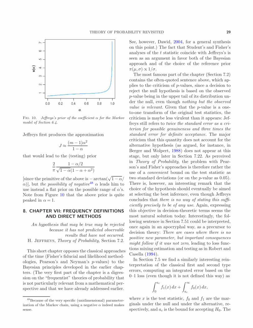
THEORY OF PROBABILITY REVISITED 29
Fig. 10. Jeffreys’s prior of the coefficient α for the Markovmodel of Section 6.4.
Jeffreys first produces the approximation
J ≈ (m− 1)α2
1−α
that would lead to the (testing) prior
2
π
1− α/2√1− α(1−α+α2)
[since the primitive of the above is −arctan(√1−α/
α)], but the possibility of negative48 α leads him touse instead a flat prior on the possible range of α’s.Note from Figure 10 that the above prior is quitepeaked in α= 1.
8. CHAPTER VII: FREQUENCY DEFINITIONS
AND DIRECT METHODS
An hypothesis that may be true may be rejectedbecause it has not predicted observable
results that have not occurred.H. Jeffreys, Theory of Probability, Section 7.2.
This short chapter opposes the classical approachesof the time (Fisher’s fiducial and likelihood method-ologies, Pearson’s and Neyman’s p-values) to theBayesian principles developed in the earlier chap-ters. (The very first part of the chapter is a digres-sion on the “frequentist” theories of probability thatis not particularly relevant from a mathematical per-spective and that we have already addressed earlier.
48Because of the very specific (unidimensional) parameter-ization of the Markov chain, using a negative α indeed makessense.
See, however, Dawid, 2004, for a general synthesison this point.) The fact that Student’s and Fisher’sanalyses of the t statistic coincide with Jeffreys’s isseen as an argument in favor both of the Bayesianapproach and of the choice of the reference priorπ(µ,σ)∝ 1/σ.The most famous part of the chapter (Section 7.2)
contains the often-quoted sentence above, which ap-plies to the criticism of p-values, since a decision toreject the null hypothesis is based on the observedp-value being in the upper tail of its distribution un-der the null, even though nothing but the observedvalue is relevant. Given that the p-value is a one-to-one transform of the original test statistics, thecriticism is maybe less virulent than it appears: Jef-freys still refers to twice the standard error as a cri-terion for possible genuineness and three times thestandard error for definite acceptance. The majorcriticism that this quantity does not account for thealternative hypothesis (as argued, for instance, inBerger and Wolpert, 1988) does not appear at thisstage, but only later in Section 7.22. As perceivedin Theory of Probability, the problem with Pear-son’s and Fisher’s approaches is therefore rather theuse of a convenient bound on the test statistic astwo standard deviations (or on the p-value as 0.05).There is, however, an interesting remark that thechoice of the hypothesis should eventually be aimedat selecting the best inference, even though Jeffreysconcludes that there is no way of stating this suffi-ciently precisely to be of any use. Again, expressingthis objective in decision-theoretic terms seems themost natural solution today. Interestingly, the fol-lowing sentence in Section 7.51 could be interpreted,once again in an apocryphal way, as a precursor todecision theory: There are cases where there is nopositive new parameter, but important consequencesmight follow if it was not zero, leading to loss func-tions mixing estimation and testing as in Robert andCasella (1994).In Section 7.5 we find a similarly interesting rein-
terpretation of the classical first and second typeerrors, computing an integrated error based on the0–1 loss (even though it is not defined this way) as
∫ ac
0f1(x)dx+
∫ ∞
ac
f0(x)dx,
where x is the test statistic, f0 and f1 are the mar-ginals under the null and under the alternative, re-spectively, and ac is the bound for acceptingH0. The
30 C. P. ROBERT, N. CHOPIN AND J. ROUSSEAU
optimal value of ac is therefore given by f0(ac) =f1(ac), which amounts to
π(H0|x= ac) = π(Hc0|x= ac),
that is,K = 1 if both hypotheses are equally weighteda priori. This is a completely rigorous derivationof the optimal Bayesian decision for testing, eventhough Jeffreys does not approach it this way, inparticular, because the prior probabilities are notnecessarily equal (a point discussed earlier in Sec-tion 6.0 for instance). It is nonetheless a fairly con-vincing argument against p-values in terms of small-est number of mistakes. More prosaically, Jeffreysbriefly discusses in this section the disturbing asym-metry of frequentist tests, when both hypotheses areof the same type: if we must choose between two def-initely stated alternatives, we should naturally takethe one that gives the larger likelihood, even thougheach may be within the range of acceptance of theother.
9. CHAPTER VIII: GENERAL QUESTIONS
A prior probability used to express ignorance ismerely the formal statement of that ignorance.
H. Jeffreys, Theory of Probability, Section 8.1.
This concluding chapter summarizes the main rea-sons for using the Bayesian perspective:
1. Prior and sampling probabilities are represen-tations of degrees of belief rather than frequencies(Section 8.0). Once again, we believe that this de-bate49 is settled today, by considering that proba-bility distributions and improper priors are definedaccording to the rules of measure theory; see, how-ever, Dawid (2004) for another perspective orientedtoward calibration.2. While prior probabilities are subjective and can-
not be uniquely assessed, Theory of Probability setsa general (objective) principle for the derivation ofprior distributions (Section 8.1). It is quite inter-esting to read Jeffreys’s defence of this point whentaking into account the fact that this book was set-ting the point of reference for constructing nonin-formative priors. Theory of Probability does little,however, toward the construction of informative pri-ors by integrating existing prior information (except
49Jeffreys argues that the limit definition was not stated tilleighty years later than Bayes, which sounds incorrect whenconsidering that the Law of Large Numbers was produced byBernoulli in Ars Conjectandi.
in the sequential case discussed earlier), recogniz-ing nonetheless the natural discrepancy between twoprobability distributions conditional on two differ-ent data sets. More fundamentally, this stresses thatTheory of Probability focuses on prior probabilitiesused to express ignorance more than anything else.3. Bayesian statistics naturally allow for model
specification and, as such, do not suffer (as much)from the neglect of an unforeseen alternative (Sec-tion 8.2). This is obviously true only to some extent:if, in the process of comparing models Mi based onan experiment, one very likely model is omitted fromthe list, the consequences may be severe. On theother hand, and in relation to the previous discus-sion on the p-values, the Bayesian approach allowsfor alternative models and is thus naturally embed-ding model specification within its paradigm.50 Thefact that it requires an alternative hypothesis to op-erate a test is an illustration of this feature.4. Different theories leading to the same poste-
riors cannot be distinguished since questions thatcannot be decided by means of observations are bestleft alone (Section 8.3). The physicists’51 conceptof rejection of unobservables is to be understood asthe elimination of parameters in a law that make nocontribution to the results of any observation or as aversion of Ockham’s principle, introducing new pa-rameters only when observations showed them to benecessary (Section 8.4). See Dawid (1984, 2004) fora discussion of this principle he calls Jeffreys’s Law.5. The theory of Bayesian statistics as presented
in Theory of Probability is consistent in that it pro-vides general rules to construct noninformative pri-ors and to conduct tests of hypotheses (Section 8.6).It is in agreement with the Likelihood Principle andwith conditioning on sufficient statistics.52 It alsoavoids the use of p-values for testing hypotheses byrequiring no empirical hypothesis to be true or false
50The point about being prepared for occasional wrong de-cisions could possibly be related to Popper’s notion of fal-sifiability : by picking a specific prior, it is always possible tomodify inference toward one’s goal. Of course, the divergencesbetween Jeffreys’s and Popper’s approaches to induction makethem quite irreconcilable. See Dawid (2004) for a Bayes–deFinetti–Popper synthesis.
51Both paragraphs Sections 8.3 and 8.4 seem only con-cerned with a physicists’ debate, particularly about the rele-vance of quantum theory.
52We recall that Fisher information is not fully compatiblewith the Likelihood Principle (Berger and Wolpert, 1988).
THEORY OF PROBABILITY REVISITED 31
a priori. However, special cases and multidimen-sional settings show that this theory cannot claimto be completely universal.6. The final paragraph of Theory of Probability
states that the present theory does not justify induc-tion; what it does is to provide rules for consistency.This is absolutely coherent with the above: althoughthe book considers many special cases and excep-tions, it does provide a general rule for conduct-ing point inference (estimation) and testing of hy-potheses by deriving generic rules for the construc-tion of noninformative priors. Many other solutionsare available, but the consistency cannot be denied,while a ranking of those solutions is unthinkable.In essence, Theory of Probability has thus mostlyachieved its goal of presenting a self-contained the-ory of inference based on a minimum of assumptionsand covering the whole field of inferential purposes.
10. CONCLUSION
It is essential to the possibility of induction that weshall be prepared for occasional wrong decisions.H. Jeffreys, Theory of Probability, Section 8.2.
Despite a tone that some may consider as overlycritical, and therefore unfair to such a pioneer in ourfield, this perusal of Theory of Probability leaves uswith the feeling of a considerable achievement to-ward the formalization of Bayesian theory and theconstruction of an objective and consistent frame-work. Besides setting the Bayesian principle in fullgenerality,
Posterior Probability ∝PriorProbability ·Likelihood ,
including using improper priors indistinctly from prop-er priors, the book sets a generic theory for selectingreference priors in general inferential settings,
π(θ)∝ |I(θ)|1/2,
as well as when testing point null hypotheses,
1
π
dJ1/2
1 + J=
1
πd{tan−1 J1/2(θ)},
when J(θ) = div{f(·|θ0), f(·|θ)} is a divergence mea-sure between the sampling distribution under thenull and under the alternative. The lack of a decision-theoretic formalism for point estimation notwith-standing, Jeffreys sets up a completely operationaltechnology for hypothesis testing and model choice
that is centered on the Bayes factor. Premises of hi-erarchical Bayesian analysis, reference priors, match-ing priors and mixture analysis can be found at var-ious places in the book. That it sometimes lacksmathematical rigor and often indulges in debatesthat may look superficial today is once again a re-flection of the idiosyncrasies of the time: even theultimate revolutions cannot be built on void andthey do need the shoulders of earlier giants to stepfurther. We thus absolutely acknowledge the depthand worth of Theory of Probability as a foundationaltext for Bayesian Statistics and hope that the cur-rent review may help in its reassessment.
ACKNOWLEDGMENTS
This paper originates from a reading seminar heldat CREST in March 2008. The authors are gratefulto the participants for their helpful comments. Pro-fessor Dennis Lindley very kindly provided light onseveral difficult passages and we thank him for histime, his patience and his supportive comments. Weare also grateful to Jim Berger and to Steve Addisonfor helpful suggestions, and to Mike Titterington fora very detailed reading of a preliminary version ofthis paper. David Aldrich directed us to his most in-formative website about Harold Jeffreys and Theoryof Probability. Parts of this paper were written dur-ing the first author’s visit to the Isaac Newton In-stitute in Harold Jeffreys’s alma mater, Cambridge,whose peaceful working environment was deeply ap-preciated. Comments from the editorial team of Sta-tistical Science were also most helpful.
REFERENCES
Aldrich, J. (2008). R. A. Fisher on Bayes and Bayes’ theo-rem. Bayesian Anal. 3 161–170. MR2383255
Balasubramanian, V. (1997). Statistical inference, Occam’srazor, and statistical mechanics on the space of probabilitydistributions. Neural Comput. 9 349–368.
Basu, D. (1988). Statistical Information and Likelihood: ACollection of Critical Essays by Dr. D. Basu. Springer, NewYork. MR0953081
Bauwens, L. (1984). Bayesian Full Information of Simulta-neous Equations Models Using Integration by Monte Carlo.Lecture Notes in Economics and Mathematical Systems232. Springer, New York. MR0766396
Bayarri, M. and Garcia-Donato, G. (2007). Extendingconventional priors for testing general hypotheses in linearmodels. Biometrika 94 135–152. MR2367828
Bayes, T. (1963). An essay towards solving a problem in thedoctrine of chances. Phil. Trans. Roy. Soc. 53 370–418.
32 C. P. ROBERT, N. CHOPIN AND J. ROUSSEAU
Beaumont, M., Zhang, W. and Balding, D. (2002). Ap-proximate Bayesian computation in population genetics.Genetics 162 2025–2035.
Berger, J. (1985). Statistical Decision Theory and BayesianAnalysis, 2nd ed. Springer, New York. MR0804611
Berger, J. and Bernardo, J. (1992). On the developmentof the reference prior method. In Bayesian Statistics 4(J. Berger, J. Bernardo, A. Dawid and A. Smith, eds.) 35–49. Oxford Univ. Press, London. MR1380269
Berger, J., Bernardo, J. and Sun, D. (2009). Natural in-duction: An objective Bayesian approach. Rev. R. Acad.Cien. Serie A Mat. 103 125–135.
Berger, J., Boukai, B. and Wang, Y. (1997). Unified fre-quentist and Bayesian testing of a precise hypothesis (withdiscussion). Statist. Sci. 12 133–160. MR1617518
Berger, J. and Jefferys, W. (1992). Sharpening Ockham’srazor on a Bayesian strop. Amer. Statist. 80 64–72.
Berger, J. and Pericchi, L. (1996). The intrinsic Bayesfactor for model selection and prediction. J. Amer. Statist.Assoc. 91 109–122. MR1394065
Berger, J., Pericchi, L. and Varshavsky, J. (1998). Bayesfactors and marginal distributions in invariant situations.Sankhya Ser. A 60 307–321. MR1718789
Berger, J., Philippe, A. and Robert, C. (1998). Es-timation of quadratic functions: Reference priors fornon-centrality parameters. Statist. Sinica 8 359–375.MR1624335
Berger, J. and Robert, C. (1990). Subjective hierarchicalBayes estimation of a multivariate normal mean: On thefrequentist interface. Ann. Statist. 18 617–651. MR1056330
Berger, J. and Sellke, T. (1987). Testing a point-null hy-pothesis: The irreconcilability of significance levels and ev-idence (with discussion). J. Amer. Statist. Assoc. 82 112–122. MR0883340
Berger, J. and Wolpert, R. (1988). The Likelihood Princi-ple, 2nd ed. IMS Lecture Notes—Monograph Series 9. IMS,Hayward.
Bernardo, J. (1979). Reference posterior distributions forBayesian inference (with discussion). J. Roy. Statist. Soc.Ser. B 41 113–147. MR0547240
Bernardo, J. and Smith, A. (1994). Bayesian Theory. Wi-ley, New York. MR1274699
Billingsley, P. (1986). Probability and Measure, 2nd ed. Wi-ley, New York. MR0830424
Broemeling, L. and Broemeling, A. (2003). Studies inthe history of probability and statistics xlviii the Bayesiancontributions of Ernest Lhoste. Biometrika 90 728–731.MR2006848
Casella, G. and Berger, R. (2001). Statistical Inference,2nd ed. Wadsworth, Belmont, CA.
Dacunha-Castelle, D. andGassiat, E. (1999). Testing theorder of a model using locally conic parametrization: Pop-ulation mixtures and stationary ARMA processes. Ann.Statist. 27 1178–1209. MR1740115
Darmois, G. (1935). Sur les lois de probabilite a estima-tion exhaustive. Comptes Rendus Acad. Sciences Paris 200
1265–1266.Dawid, A. (1984). Present position and potential develop-
ments: Some personal views. Statistical theory. The pre-
quential approach (with discussion). J. Roy. Statist. Soc.Ser. A 147 278–292. MR0763811
Dawid, A. (2004). Probability, causality and the empiricalworld: A Bayes–de Finetti–Popper–Borel synthesis. Statist.Sci. 19 44–57. MR2082146
Dawid, A., Stone, N. and Zidek, J. (1973). Marginal-ization paradoxes in Bayesian and structural inference(with discussion). J. Roy. Statist. Soc. Ser. B 35 189–233.MR0365805
de Finetti, B. (1974). Theory of Probability, vol. 1. Wiley,New York.
de Finetti, B. (1975). Theory of Probability, vol. 2. Wiley,New York.
DeGroot, M. (1970). Optimal Statistical Decisions.McGraw-Hill, New York. MR0356303
DeGroot, M. (1973). Doing what comes naturally: In-terpreting a tail area as a posterior probability or asa likelihood ratio. J. Amer. Statist. Assoc. 68 966–969.MR0362639
Diaconis, P. and Ylvisaker, D. (1985). Quantifying prioropinion. In Bayesian Statistics 2 (J. Bernardo, M. De-Groot, D. Lindley and A. Smith, eds.) 163–175. North-Holland, Amsterdam. MR0862481
Earman, J. (1992). Bayes or Bust. MIT Press, Cambridge,MA. MR1170349
Feller, W. (1970). An Introduction to Probability Theoryand Its Applications, vol. 1. Wiley, New York.
Feller, W. (1971). An Introduction to Probability Theoryand Its Applications, vol. 2. Wiley, New York. MR0270403
Fienberg, S. (2006). When did Bayesian inference become“Bayesian”? Bayesian Anal. 1 1–40. MR2227361
Ghosh, M. and Meeden, G. (1984). A new Bayesian analysisof a random effects model. J. Roy. Statist. Soc. Ser. B 43
474–482. MR0790633Good, I. (1962). Theory of Probability by Harold Jeffreys. J.
Roy. Statist. Soc. Ser. A 125 487–489.Good, I. (1980). The contributions of Jeffreys to Bayesian
statistics. In Bayesian Analysis in Econometrics andStatistics: Essays in Honor of Harold Jeffreys 21–34.North-Holland, Amsterdam. MR0576546
Gourieroux, C. and Monfort, A. (1996). Statistics andEconometric Models. Cambridge Univ. Press.
Gradshteyn, I. and Ryzhik, I. (1980). Tables of Integrals,Series and Products. Academic Press, New York.
Haldane, J. (1932). A note on inverse probability. Proc.Cambridge Philos. Soc. 28 55–61.
Huzurbazar, V. (1976). Sufficient Statistics. Marcel Dekker,New York.
Jaakkola, T. and Jordan, M. (2000). Bayesian parameterestimation via variational methods. Statist. Comput. 10 25–37.
Jeffreys, H. (1931). Scientific Inference, 1st ed. CambridgeUniv. Press.
Jeffreys, H. (1937). Scientific Inference, 2nd ed. CambridgeUniv. Press.
Jeffreys, H. (1939). Theory of Probability, 1st ed. TheClarendon Press, Oxford.
Jeffreys, H. (1948). Theory of Probability, 2nd ed. TheClarendon Press, Oxford.
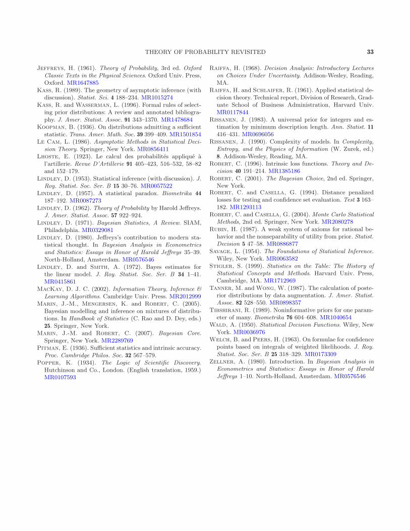
THEORY OF PROBABILITY REVISITED 33
Jeffreys, H. (1961). Theory of Probability, 3rd ed. OxfordClassic Texts in the Physical Sciences. Oxford Univ. Press,Oxford. MR1647885
Kass, R. (1989). The geometry of asymptotic inference (withdiscussion). Statist. Sci. 4 188–234. MR1015274
Kass, R. and Wasserman, L. (1996). Formal rules of select-ing prior distributions: A review and annotated bibliogra-phy. J. Amer. Statist. Assoc. 91 343–1370. MR1478684
Koopman, B. (1936). On distributions admitting a sufficientstatistic. Trans. Amer. Math. Soc. 39 399–409. MR1501854
Le Cam, L. (1986). Asymptotic Methods in Statistical Deci-sion Theory. Springer, New York. MR0856411
Lhoste, E. (1923). Le calcul des probabilites applique al’artillerie. Revue D’Artillerie 91 405–423, 516–532, 58–82and 152–179.
Lindley, D. (1953). Statistical inference (with discussion). J.Roy. Statist. Soc. Ser. B 15 30–76. MR0057522
Lindley, D. (1957). A statistical paradox. Biometrika 44
187–192. MR0087273Lindley, D. (1962). Theory of Probability by Harold Jeffreys.
J. Amer. Statist. Assoc. 57 922–924.Lindley, D. (1971). Bayesian Statistics, A Review. SIAM,
Philadelphia. MR0329081Lindley, D. (1980). Jeffreys’s contribution to modern sta-
tistical thought. In Bayesian Analysis in Econometricsand Statistics: Essays in Honor of Harold Jeffreys 35–39.North-Holland, Amsterdam. MR0576546
Lindley, D. and Smith, A. (1972). Bayes estimates forthe linear model. J. Roy. Statist. Soc. Ser. B 34 1–41.MR0415861
MacKay, D. J. C. (2002). Information Theory, Inference &Learning Algorithms. Cambridge Univ. Press. MR2012999
Marin, J.-M., Mengersen, K. and Robert, C. (2005).Bayesian modelling and inference on mixtures of distribu-tions. In Handbook of Statistics (C. Rao and D. Dey, eds.)25. Springer, New York.
Marin, J.-M. and Robert, C. (2007). Bayesian Core.Springer, New York. MR2289769
Pitman, E. (1936). Sufficient statistics and intrinsic accuracy.Proc. Cambridge Philos. Soc. 32 567–579.
Popper, K. (1934). The Logic of Scientific Discovery.Hutchinson and Co., London. (English translation, 1959.)MR0107593
Raiffa, H. (1968). Decision Analysis: Introductory Lectureson Choices Under Uncertainty. Addison-Wesley, Reading,MA.
Raiffa, H. and Schlaifer, R. (1961). Applied statistical de-cision theory. Technical report, Division of Research, Grad-uate School of Business Administration, Harvard Univ.MR0117844
Rissanen, J. (1983). A universal prior for integers and es-timation by minimum description length. Ann. Statist. 11416–431. MR0696056
Rissanen, J. (1990). Complexity of models. In Complexity,Entropy, and the Physics of Information (W. Zurek, ed.)8. Addison-Wesley, Reading, MA.
Robert, C. (1996). Intrinsic loss functions. Theory and De-cision 40 191–214. MR1385186
Robert, C. (2001). The Bayesian Choice, 2nd ed. Springer,New York.
Robert, C. and Casella, G. (1994). Distance penalizedlosses for testing and confidence set evaluation. Test 3 163–182. MR1293113
Robert, C. and Casella, G. (2004). Monte Carlo StatisticalMethods, 2nd ed. Springer, New York. MR2080278
Rubin, H. (1987). A weak system of axioms for rational be-havior and the nonseparability of utility from prior. Statist.Decision 5 47–58. MR0886877
Savage, L. (1954). The Foundations of Statistical Inference.Wiley, New York. MR0063582
Stigler, S. (1999). Statistics on the Table: The History ofStatistical Concepts and Methods. Harvard Univ. Press,Cambridge, MA. MR1712969
Tanner, M. andWong, W. (1987). The calculation of poste-rior distributions by data augmentation. J. Amer. Statist.Assoc. 82 528–550. MR0898357
Tibshirani, R. (1989). Noninformative priors for one param-eter of many. Biometrika 76 604–608. MR1040654
Wald, A. (1950). Statistical Decision Functions. Wiley, NewYork. MR0036976
Welch, B. and Peers, H. (1963). On formulae for confidencepoints based on integrals of weighted likelihoods. J. Roy.Statist. Soc. Ser. B 25 318–329. MR0173309
Zellner, A. (1980). Introduction. In Bayesian Analysis inEconometrics and Statistics: Essays in Honor of HaroldJeffreys 1–10. North-Holland, Amsterdam. MR0576546