happiness productivity
DESCRIPTION
Report on relationship between happiness and productivity.TRANSCRIPT
Happiness and Productivity
Andrew J. Oswald*, Eugenio Proto**, and Daniel Sgroi**
*University of Warwick, UK, and IZA Bonn, Germany
**University of Warwick, UK
JOLE 3rd Version: 10 February 2014
Emails: [email protected]; [email protected]; [email protected] JEL Classification: D03, J24, C91 Keywords: Well-being; productivity; happiness; personnel economics. Address: Department of Economics, University of Warwick, Coventry CV4 7AL, United Kingdom. Telephone: (+44) 02476 523510 Acknowledgements: For their suggestions, we thank the referees and the editor Paul Oyer. For fine research assistance, and valuable discussions, we are indebted to Malena Digiuni, Alex Dobson, Stephen Lovelady, and Lucy Rippon. For advice, we would like to record our deep gratitude to Alice Isen. Insightful suggestions were provided by seminar audiences in Berlin, Birmingham, Bonn, Leicester, Glasgow, HM Treasury London, LSE, Maastricht, PSE Paris, Warwick, York, and Zurich. Special thanks also go to Johannes Abeler, Eve Caroli, Emanuele Castano, Andrew Clark, Alain Cohn, Ernst Fehr, Justina Fischer, Bruno Frey, Dan Gilbert, Amanda Goodall, Greg Jones, Graham Loomes, Rocco Macchiavello, Michel Marechal, Sharun Mukand, Steve Pischke, Nick Powdthavee, Tommaso Reggiani, Daniel Schunk, Claudia Senik, Tania Singer, and Luca Stanca. The first author thanks the University of Zurich for its hospitality and is grateful to the ESRC for a research professorship. The ESRC (through CAGE) and the Leverhulme Trust also provided research support.
1
Abstract
Some firms say they care about the well-being and ‘happiness’ of their employees. But are such
claims hype, or scientific good sense? We provide evidence, for a classic piece-rate setting, that
happiness makes people more productive. In three different styles of experiment, randomly selected
individuals are made happier. The treated individuals have approximately 12% greater productivity.
A fourth experiment studies major real-world shocks (bereavement and family illness). Lower
happiness is systematically associated with lower productivity. These different forms of evidence,
with complementary strengths and weaknesses, are consistent with the existence of a causal link
between human well-being and human performance.
2
At Google, we know that health, family and wellbeing are an important aspect of Googlers’ lives. We have also noticed that employees who are happy ... demonstrate increased motivation ... [We] ... work to ensure that Google is... an emotionally healthy place to work. Lara Harding, People Programs Manager, Google.
Supporting our people must begin at the most fundamental level – their physical and mental health and well-being. It is only from strong foundations that they can handle ... complex issues. Matthew Thomas, Manager – Employee Relations, Ernst and Young. Quotes from the report Healthy People = Healthy Profits Source: http://www.dwp.gov.uk/docs/hwwb-healthy-people-healthy-profits.pdf
1. Introduction
This study explores a question of interest to economists, behavioral scientists, employers, and
policy-makers. Does ‘happiness’ make human beings more productive? Consistent with claims such
as those in the above quote from the Google corporation, we provide evidence that it does. We show
this in a piece-rate setting1 with otherwise well-understood properties (our work uses the timed
mathematical-additions task of Niederle and Vesterlund 2007). In a series of experiments, we
experimentally assign happiness in the laboratory and also exploit data on major real-life
(un)happiness shocks.2 This combination makes it possible to consider the distinction3 between long-
term well-being and short-term positive ‘affect’. The sample size in our study, which proceeded over
a number of years, is 713 individuals. Mean productivity in our entire sample is just under 20 correct
additions. The happiness treatments improve that productivity by approximately 2 additions, namely,
by approximately 10%-12%.
The study’s key result is demonstrated in four ways. Each of these employs a different form of
experiment (numbered I, II, III, and IV). All the laboratory subjects are young men and women who
attend an elite English university with required entry grades amongst the highest in the country.
In Experiment I, a comedy movie clip is played to a group of subjects. Their later measured
productivity on a standardized task is found to be substantially greater than in groups of control
subjects who did not see the clip. This result is a simple cross-sectional one. However, the finding
has a causal interpretation because it rests on a randomized treatment. In Experiment II, a comedy
clip is again used. This time, however, repeated longitudinal measurements are taken. The greatest
productivity boost is shown to occur among the subjects who experience the greatest improvement in
happiness. In Experiment III, a different treatment -- at the suggestion of an editorial reader of this
journal -- is adopted. In an attempt to mirror somewhat more closely, admittedly still in a stylized
way, the sort of policies that might potentially be provided by actual employers, our treatment
subjects are provided with chocolate, fruit, and drinks. As before, a positive productivity effect is
produced, and again the size of that effect is substantial. In a fourth trial, Experiment IV, subjects’
productivities are measured at the very outset. At the end of the experiment, these subjects are
1 Such as Niederle and Vesterlund (2007). 2 The relevance of this effect is witnessed by a business-press literature suggesting that employee happiness is a common goal in firms, with the expectation that happier people are more productive. The formal economics literature has contributed relatively little to this discussion. 3 A distinction emphasized in Lyubomirsky et al. (2005).
3
quizzed, by questionnaire, about recent tragedies in their families’ lives (a kind of unhappy
randomization by Nature, rather than by us, it might be argued). Those who report tragedies at the
end of the laboratory trial are disproportionately ones who had significantly lower productivity at its
start. Those individuals also report lower happiness. One caveat should be mentioned. Although our
work suggests that happier workers are more productive, we cannot, as a rule, say that real-world
employers should expend more resources on making their employees happier. In some of the
experiments described below, half of the time in the laboratory was spent in raising the subjects’
happiness levels, and in one of the other experiments we spent approximately two dollars per person
on fruit and chocolate to raise productivity by almost 20% for a short period of concentrated work.
This study illustrates the existence of a potentially important mechanism. However, it cannot
adjudicate, and is not designed to adjudicate, on the net benefits and costs within existing business
settings (although it suggests that research in such settings would be of interest).
To our knowledge, this study is the first to have the following set of features4. We implement a
monetary piece-rate setup. We examine large real-world shocks to happiness and not solely small
laboratory ones. Using a range of different experimental designs, we offer various types of evidence.
We also collect longitudinal data in a way that provides us with an opportunity to scrutinize the
changes in happiness within our subjects. In a more strictly psychological tradition, research by the
late Alice Isen of Cornell University has been important in this area. The closest previous paper to
our own is arguably Erez and Isen (2002). Those authors wish to assess the impact of positive affect
on motivation. In their experiment, 97 subjects -- half of them mood-manipulated by the gift of a
candy bag-- are asked to solve 9 anagrams (three of which are unsolvable) and are rewarded with the
chance of a lottery prize. Their framework might perhaps be seen as an informal kind of piece-rate
set-up. The subjects who receive the candy solve more anagrams. In later work, Isen and Reeve
(2005) demonstrate that positive well-being induces subjects to change their allocation of time
towards more interesting tasks, and that, despite this, the subjects retain similar levels of performance
in the less interesting tasks. More generally, it is now known that positive well-being can influence
the capacities of choice and innovative content.5 That research has concentrated on unpaid
experimental settings. 6
The background to our project is that there is a large literature on productivity at the personal and
plant level (for example, Caves 1974, Lazear 1981, Ichniowski and Shaw 1999, Siebert and Zubanov
2010, Segal 2012). There is a growing one on the measurement of human well-being (for example,
4 We are conscious that this is difficult to determine unambiguously, especially on a topic that crosses various social-science disciplines, so we should say that the judgment is made as best we can after literature searches and having had the paper read by a number of economists, psychologists, and management researchers. 5 A body of related empirical research by psychologists has existed for some years. We list a number of them in the paper’s references; these include Argyle (1989), Ashby et al. (1999), and Isen (2000). See also Amabile et al. (2005). The work of Wright and Staw (1998) examines the connections between worker well-being and supervisors’ ratings of workers. The authors find mixed results. Our study also links to ideas in the broaden-and-build approach of Frederickson and Joiner (2002) and to material examined in Lyubomirsky et al. (2005). 6 See also the non piece-rate work of Baker et al. (1997), Estrada et al. (1997), Forgas (1989), Jundt and Hinsz ( 2001), Kavanagh (1987), Melton (1995), Patterson et al. (2004), Sanna et al. (1996), Sinclair and Mark (1995), Steele and Aronson (1995), Tsai et al. (2007), and Zelenski et al. (2008).
4
Easterlin 2003, Van Praag and Ferrer-I-Carbonell 2004, Layard 2006, Ifcher and Zarghamee 2011,
Benjamin et al. 2012). Yet economists and management scientists still know relatively little about the
causal linkages between these two variables. Empirically, our work connects to, and might eventually
offer elements of a microeconomic foundation for, the innovative recent study by Edmans (2012),
who finds that levels of job satisfaction appear to be predictive of future stock-market performance.
Similarly, Bockerman and Ilmakunnas (2012) show in longitudinal European data that, with
instrumental-variables estimation, an increase in the measure of job satisfaction by one within-plant
standard deviation increases value-added per hours worked in manufacturing by 6.6%. Conceptually,
our work relates to Bewley (1999), who finds that firms cite likely loss of morale as the reason they
do not cut wages, and to Dickinson (1999), who provides evidences that an increase of a piece-rate
wage can decrease hours but increase labor intensity, and also to Banerjee and Mullainathan (2008),
who consider a model where labor intensity depends on outside worries and this generates a form of
non-linear dynamics between wealth and effort. Recent work by Segal (2012) also distinguishes
between two underlying elements of motivation. Gneezy and Rustichini (2000) show that an increase
in monetary compensation raises performance, but that offering no monetary compensation can be
better than offering some.7 Such writings reflect an increasing interest among economists in how to
reconcile external incentives with intrinsic forces such as self-motivation.8 Our work may also
eventually offer a potential explanation for the reverse longitudinal finding, using young Americans’
earnings from the Add Health data set, of De Neve and Oswald (2012).
We draw upon empirical ideas and methods used in sources such as Kirchsteiger, Rigotti and
Rustichini (2006) and Ifcher and Zarghamee (2011). Our paper lends theoretical support to concepts
emphasized by Kimball and Willis (2006) and Benjamin et al. (2012). A key idea is that happiness
may be an argument of the utility function. 9 Like Oswald and Wu (2010) -- who show as a validation
of life-satisfaction data that for the US states there is a match with the objective pattern implied by
spatial compensating differentials theory -- this study’s later results are consistent with the view that
there is genuine informational content in well-being data.
The paper concentrates on regression equations. An appendix lays out graphical demonstrations of
some of the study’s key results; this is because our points can be made with elementary t-tests, and
because we hope they might interest behavioral scientists who do not work with the style of
regression equation favored by economists. The appendix also contains a range of robustness checks.
2. A Series of Experiments
Four kinds of experiment were done and each produced evidence consistent with the idea that
7 See also Benabou and Tirole (2003), who examine the relationship between both types of motivation. 8 Diener et al. (1999) reviews the links between choices and emotional states. 9 A considerable literature in economics has studied happiness and wellbeing as a dependent variable – including Blanchflower and Oswald (2004), Clark et al. (2008), Di Tella et al. (2001), Frey and Stutzer (2002), Luttmer (2005), Senik (2004), Powdthavee (2010), and Winkelmann and Winkelmann (1998). See Freeman (1978) and Pugno and Depedri (2009) on job satisfaction and work performance. Other relevant work includes Compte and Postlewaite (2004).
5
‘happier’ workers are intrinsically more productive. In total, more than seven hundred subjects took
part in the trials.10 The experimental instructions, the layout of a GMAT-style math test, and the
questionnaires are explained in the appendix.
The experiments deliberately varied in their design. Here we list the main features upon which we
draw. In different experiments, we chose different combinations of the following features:
Feature 1: An initial questionnaire when the person arrived in the laboratory. This asked: How
would you rate your happiness at the moment? Please use a 7-point scale where 1 is completely sad,
2 is very sad, 3 is sad, 4 is neither happy nor sad, 5 is fairly happy, 6 is very happy and 7 is
completely happy.
Feature 2: A mood-induction procedure that changed the person’s happiness. In two cases this
was done by showing movie clips. This procedure was used in Experiments I and II. The treatment
was a 10-minute clip of sketches in which there are jokes told by a well-known comedian.11 As a
control, we used either a calm “placebo” clip or no clip.12 We also checked one alternative. In that
further case, Experiment III, the treated subjects were instead provided with fruit, chocolate, and
bottled drinks.
Feature 3: A mid-experiment questionnaire. This asked the person’s happiness immediately after
the movie clip.
Feature 4: A task designed to measure productivity. We borrowed ours from Niederle and
Vesterlund (2007). The subjects were asked to answer correctly as many different additions of five 2-
digit numbers as possible in 10 minutes. This task is simple but is taxing under pressure. We think of
it as representing -- admittedly in a stylized way -- a white-collar job: both intellectual ability and
effort are rewarded. The laboratory subjects were allowed to use pen and paper, but not a calculator or
similar. Each subject had a randomly designed sequence of these arithmetical questions and was paid
at a rate of £0.25 per correct answer. Numerical additions were undertaken directly through a
protected Excel spreadsheet, with a typical example as in Legend 1.
31 56 14 44 87 Total =
Legend 1: Adding Five 2-digit Numbers under Timed Pressure
Feature 5. A short GMAT-style math test. This had 5 questions along similar lines to that of
Gneezy and Rustichini (2000). Subjects had 5 minutes to complete this and were paid at a rate of
£0.50 per correct answer. To help to disentangle effort from ability, we used this test to measure
underlying ability.13
10 All were university students, as is common in the literature. 11 The questionnaire results indicate that the clip was generally found to be entertaining and had a direct impact on reported happiness levels. We also have direct evidence that the clip raised happiness through a comparison of questionnaire happiness reports directly before and after the clip. 12 See James Gross's resources site (http://www-psych.stanford.edu/~psyphy/movs/computer_graphic.mov) for the clip we used as a placebo. 13 We deliberately kept the number of GMAT MATH-style questions low. This was to try to remove any effort component from the task so as to keep it a cleaner measure of raw ability: 5 questions in 5 minutes is a relatively generous amount of time for an IQ-based test, and
6
Feature 6. A final questionnaire. This took two possible forms. It was either (a) a last happiness
report of the exact same wording as in the first questionnaire and further demographic questions or (b)
the same as (a) plus a number of questions designed to reveal any bad life event(s) (henceforth BLE)
that had taken place in the last 5 years for the subject. Crucially, we requested information about
these life events at the end of the experiment. This was to ensure that the questions would not,
through a priming effect, influence reported happiness measures taken earlier in the experiment. The
final questionnaire included a measure of prior exposure to mathematics and school exam
performance, which we could also use as controls to supplement the GMAT results from feature 5.
The precise elements in each experimental session differed depending upon the specific aim. They
can be grouped into four:
• “Experiment I” on short-run happiness shocks, induced by a movie clip, within the
laboratory;
• “Experiment II” which was similar but also asked happiness questions throughout the lab
experiment;
• “Experiment III” using a different form of short-happiness shock (fruit, chocolate, drinks)
in the laboratory.
• “Experiment IV” on severe happiness shocks from the real-world.
We randomly assigned subjects to different treatments. No subject took part in more than a single
experiment; individuals were told that the tasks would be completed anonymously; they were asked to
refrain from communication with each other; they were told not to use electronic devices for
assistance. Subjects were told in advance that there would be a show-up fee (of £5) and the likely
range of bonus (performance-related) payments (typically up to a further £20 for the hour’s work).
Following the economist’s tradition, a reason to pay subjects more for correct answers was to
emphasize they would benefit from higher performance. We wished to avoid the idea that they might
be paying back effort -- as in a kind of ‘reciprocity’ effect -- to investigators. That concern is not
relevant in Experiment IV because productivity was measured before the question on bad life events.
2a. Experiment I: Mood Induction and Short-run Happiness Shocks
In Experiment I, we used a short-run happiness shock, namely a comedy clip, within the laboratory
(feature 2 in the earlier list). The control-group individuals were not present in the same room with
the treated subjects; they never overheard laughter or had any other interaction. The experiment was
carried out with deliberate alternation of the early and late afternoon slots. This was to avoid time-of-
day effects.
casual observation indicated that subjects did not have any difficulty giving some answers to the GMAT MATH-style questions, often well within the 5-minute deadline.

7
Here we use features 2, 4, 5 and 6(a) from the Features list.14 The final questionnaire inquired into
both the happiness level of subjects (before and after the clip for treatment 1), and their level of
mathematical expertise. In day 5 and day 6, we added extra questions (as detailed in the appendix) to
the final questionnaire. These were a check designed to inquire into subjects’ motivations and their
own perceptions of what was happening to them. The core sessions took place over 4 days. We then
added 4 more sessions in two additional days designed to check for the robustness of the central result
to the introduction of an explicit payment and a placebo film (shown to the otherwise untreated
group).
Subjects received £0.25 per correct answer on the arithmetic task and £0.50 on each correct
GMAT-style math answer, and this was rounded up to avoid the need to give them large numbers of
coins as payment.
We used two different forms of wording:
• For days 1-4 we did not specify exact details of payments, although we communicated clearly
to the subjects that the payment did depend heavily on performance.
• For days 5-6 the subjects were told the explicit rate of pay both for the numerical additions
(£0.25 per correct answer) and GMAT-style math questions (£0.50 per correct answer).
This achieved several things. First, in the latter case we have a revealed-payment setup, which is a
proxy for many real-world piece-rate contracts (days 5-6), and in the former we mimic those
situations in real life where workers do not have a contract where they know the precise return from
each productive action they take (days 1-4). Second, this difference provides the opportunity to check
that the wording of the payment method does not have a significant effect -- thereby making one set
of days a robustness check on the other.
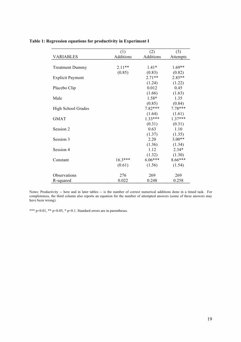
In Experiment I, 276 subjects participated. Here we present the results of the 4 basic sessions of
this experiment. Our productivity variable in the analysis is the number of correct additions in the
allotted ten minutes. It has a mean of 17.40. The key independent variable is whether or not a person
observed the happiness movie clip.15
Our results point to the existence of a positive association between human happiness and human
productivity. The findings can be illustrated in regressions or graphically. Here, in column 1 of Table
1, the treated group’s mean performance in Experiment I is higher by 2.11 additions than the
performance of the control group. This productivity difference is approximately thirteen percent. It is
significantly different from zero (p=0.02). As shown in the figures of the appendix, male and female
groups have a similar increment in their productivity. One sub-group was noticeable in the data.
14 In this experiment, we choose not to measure the happiness level at the beginning; this is to avoid the possibility that subjects treated with the comedy clip could guess the nature of the experiment. 15 Our movie clip is successful in increasing the happiness levels of subjects. The subjects report an average rise of almost one point on the scale of 1 to 7. Moreover, comparing the ex-post happiness of the treated subjects with that of the non-treated subjects, we observe that the average of the former is higher by 0.85 points. Using a two-sided t-test, this difference is statistically significant (p <0.01). Finally, it is useful to notice that the reported level of happiness before the clip for the treated group is not statistically significantly different (the difference is just 0.13) from the happiness of the untreated group (p = 0.20 on the difference).

8
Encouragingly for our account, the performance of those 16 subjects in the treated group who did not
report an increase in happiness is not statistically different from the performance of the untreated
group (p=0.67). The increase in performance thus seems to be linked to the rise in happiness rather
than merely to the fact of watching a movie clip. However, we return to this issue later and examine
it more systematically.
We perform a set of robustness tests, in the later columns of Table 1’s regression equations, to
provide a check on both the inclusion of a placebo clip and explicit payment, and we report also an
‘attempts’ equation. A range of covariates are added as additional independent variables. In column
2 of Table 1, the estimated size of the effect is now approximately 1.4, and the standard error has
increased. Within this data set, there are two extreme outliers, and if these are excluded then the
standard error on this treatment coefficient is considerably smaller. Nevertheless, we prefer to report
the full-sample results and to turn to additional experiments to probe the strength of the current
finding.
2b. Experiment II: Before-and-After Happiness Measurements in the Laboratory
In Experiment I it is not possible to observe in real time -- although they are asked some
retrospective questions -- the happiness levels of individuals before and after the comedy movie clip.
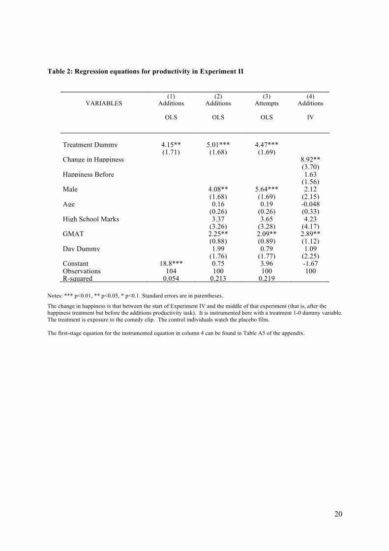
To deal with this, we designed Experiment II. A group of 52 males and 52 females participated.
Differently from the other experiment, we ask happiness questions before playing the movie clip, and
then longitudinally. The appendix describes the data.
We asked subjects about their happiness level on three occasions. The initial measurement was at
the very start of the experiment. The second was immediately after the comedy or placebo film. The
third time was at the end of the experiment. Experiment II used explicit payment instructions and a
placebo clip (without a placebo clip there would have been no gap between features 1 and 3 for the
control subjects). The timeline was thus features 1, 2, 3, 4, 5 and 6(a) from the earlier list. The
appendix provides further details.
In Experiment II, the individuals exposed to the comedy clip made 22.96 correct additions; those
in the control group, who watched only a calm placebo film, scored 18.81. This difference of 4.15
additions in column 1 of Table 2 is significantly different from zero (p-value< 0.01). The effect is
found in both genders, although is larger among men. The number of attempts made -- as in column 3
of Table 2 -- is significantly higher among the individuals treated with the comedy clip (p-value =
0.018). In contrast to Experiment I, in this second experiment the precision is slightly higher among
the individuals treated with the comedy clip, namely 0.88, than in individuals treated with the
placebo, 0.83. This difference, shown in column 4 of Table 2, is statistically significant (p-value
0.03). The structure of the formal regression equations in Table 2 provides information about the
determinants of subjects’ productivity in this experiment.
However, is it really extra happiness that causes the enhanced productivity?
9
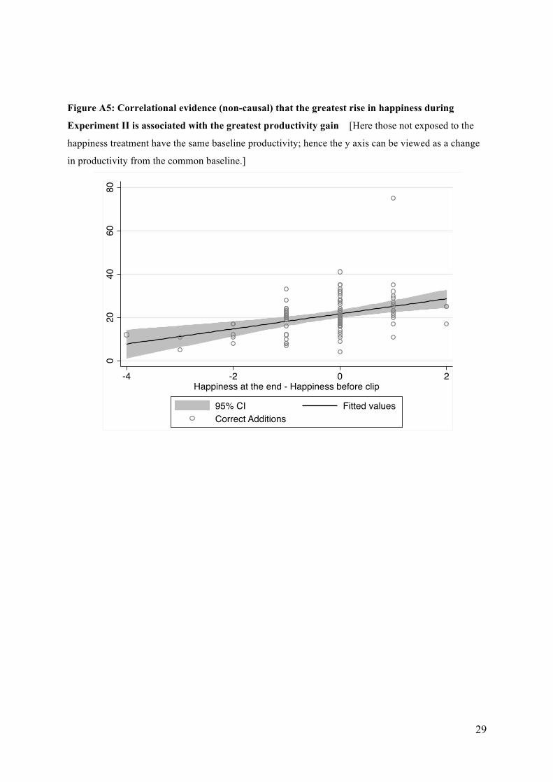
The nature of Experiment II makes it possible to check. Because people are randomly assigned to
the treatment group, we know that the baseline levels of productivity of the treatment and control
group are identical. It is therefore possible to find out, for these laboratory subjects, whether there is
link between their measured rise in happiness and the measured implied effect on productivity. We
report a simple plot, in the appendix, for the full changes. A more formal test, using data on the mid-
point reading of happiness, is in Table 2. Here we have to instrument the change in happiness,
because that change is endogenous. Under the null hypothesis, the treatment dummy variable is itself
an appropriate instrumental variable.
Column 4 of Table 2 shows that the change in happiness -- here between the start and middle of
the experiment -- is positive and statistically significant in an equation for the number of correct
additions. The key coefficient is 8.92 with a standard error of 3.70. This implies that a (large) one-
point rise in happiness would be associated with almost 9 extra correct answers in the productivity
task. Table A5 in the appendix demonstrates that, as might be expected, the comedy-clip treatment
does lead to greater reported happiness in the subjects.
Finally, it should be explained that these two experiments’ conclusions are unaffected by omitting
the use of GMAT scores as a control variable. They are also unaffected by the use or not of a calm
placebo film.
2c. Experiment III: Mood Induction and Other Kinds of Short-run Happiness Shocks
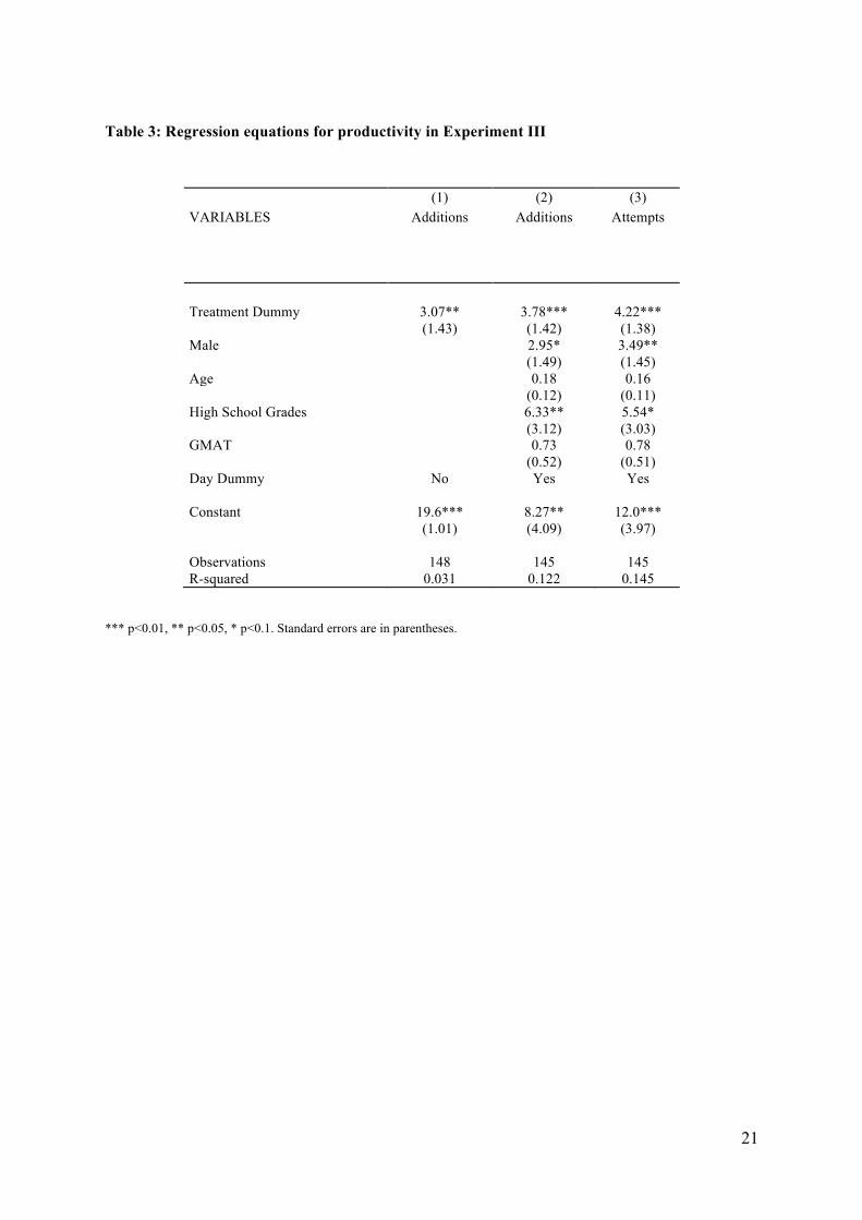
On the suggestion of an editorial reader, we ran a further trial, Experiment III. This variant used
food and drink ‘shocks’. The underlying idea is that such interventions are of a kind that would, in
principle, be more easily implementable in a commercial organization (more easily, one might say,
than getting a comedian to tell jokes in the factory at 8am every morning). In November 2013,
therefore, we performed a variation on Experiment I. This was with an additional 148 participants.
Rather than using a comedy clip as the treatment to induce happiness, we offered a selection of snacks
and drinks to the treatment group (comprising 74 subjects in 4 sessions). We provided none for the
control group (who were a different set of 74 individuals, also in 4 sessions).
For these four treatment sessions, a table was first laid with a variety of snacks (several large
bowls full of miniature chocolate bars from the Cadbury’s Heroes and Mars Celebrations range and
various different types of fruit) together with bottled spring water. The participants were then invited
to take from the snacks and water, and sit for 10 minutes to eat/drink immediately after registration
and just prior to the start of the main experiment. This 10 minutes mirrored the same 10 minutes of
time spent watching the comedy clip in the main Experiment I. The instructions were identical to
those in Experiment I except for the addition of two lines. First, individuals were invited to take from
the table on entry (“Please help yourself to the snacks and water that have been provided which you
are free to consume before the experiment begins.”). Second, just prior to the experimental
instructions, they were told: “Please now stop eating or drinking until the end of the experiment where
10
you will be free to continue partaking of any snacks you picked up as you entered”. For the four
control sessions, we invited participants to enter but there was no availability of snacks or bottled
water. They were still asked to sit for 10 minutes prior to the experiment beginning; this was to
ensure that any effect was not due to the additional minutes of experimental time for the treated
group.
Other than the treatment being different, the key features of Experiment I were retained: the
participants were first asked to carry out the numerical additions, then undertake the GMAT math-
style test, and finally complete a questionnaire. There were two minor alterations. First, the
questionnaire for the treated participants asked afterwards whether the provided snacks and water had
an effect on their happiness (instead of asking the same question about the comedy clip as in the main
Experiment I). Second, the payment rates were made explicit (at 25p per correct addition and 50p per
correct GAMT math-style answer) as in the explicit payment variation on Experiment I.
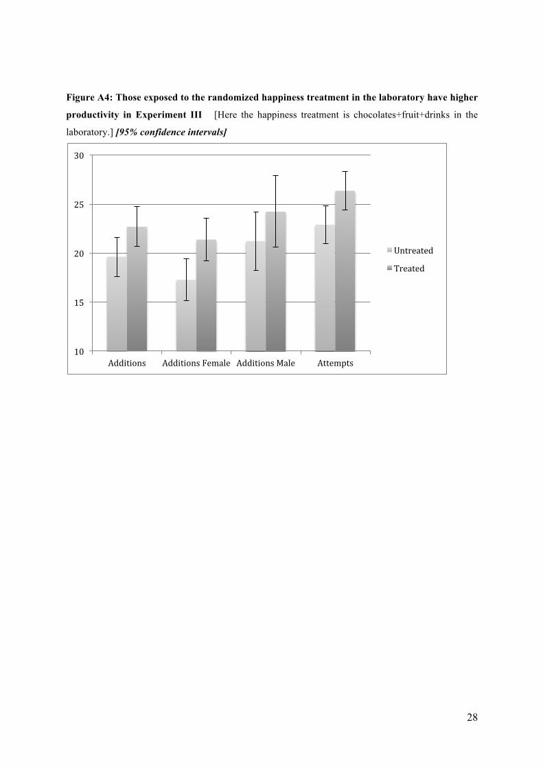
As in the previous experiments, productivity was higher in the treatment group. The results are
illustrated in Table 3. For example, in column 1 of Table 3, the productivity difference is 3.07 extra
correct additions, which is a boost to the number of correct numerical additions of approximately
15%. The increase is even larger, in column 2, when additional independent variables are included.
Column 3 of Table 3 reveals that a strong effect comes through also in the sheer number of attempts
made by laboratory participants (by 4.22 with a standard error of 1.38). We checked also that the
chocolate-fruit treatment did raise participants’ reported happiness.
Relative to the price of fruit and chocolate, which came in our experiment to the equivalent of
approximately 2 dollars per person within the laboratory, the observed boost in productivity may or
may not be large enough to make it possible to think of the extra happiness as paying for itself. The
reason is a cautionary one. It is that, although the results in Table 3 suggest that this particular
intervention increases people’s productivity by a sizeable 15-20%, it is not possible here to be sure
how long such productivity boosts would persist in a real-world setting. If this were to translate in a
lasting way into the busy offices of the real world -- as Google’s spokesperson apparently believes --
it could be expected to outweigh the additional costs. If the boost is a short-lasting one, however, it
could not. This issue seems to demand attention in future research.
2d. Experiment IV: Family Tragedies as Real-life Happiness Shocks
The preceding sections have studied small happiness interventions. For ethical reasons, it is not
feasible in experiments to induce huge changes in the happiness of people’s lives. Nevertheless, it is
possible to exploit data on the naturally occurring shocks of life. In Experiment IV we study real-life
unhappiness events assigned by Nature rather than by us. These shocks -- for which we use the
generic term Bad Life Events -- are family tragedies such as recent bereavement.
The design here uses a short questionnaire asking for people’s happiness; then we initiate the
productivity task; then there is GMAT-style math test to check people’s background mathematical
11
ability; then we finish with a questionnaire. Hence we use features 1, 4, 5 and 6(b) from the earlier
Features list. One aspect is particularly important. In this experiment we asked subjects to report
their level of happiness right at the start of the experimental session. This was to avoid ‘priming’
problems. The underlying logic is that we wanted to see if people’s initial happiness answers could
be shown to be correlated with the individuals’ later answers and behavior.
We informed the subjects of the precise payment system prior to features 4 and 5 (amounts £0.25
and £0.50 per correct answer, respectively). The final questionnaire included supplementary
questions designed to find out whether they had experienced at least one of the following BLEs: close
family bereavement, extended family bereavement, serious life-threatening illness in the close family,
and/or parental divorce. Although we did not know it when we designed our project, the idea of
examining such events has also been followed in interesting work on CEOs by Bennedsen et al.
(2010), who suggest that company performance may be impeded by traumatic family events.
Again all the laboratory subjects were young men and women who attend an elite English
university. Compared to any random slice of an adult population, they are thus -- usefully for our
experiment -- rather homogenous individuals. Those among them who have experienced family
tragedies are, to the outside observer, approximately indistinguishable from the others.
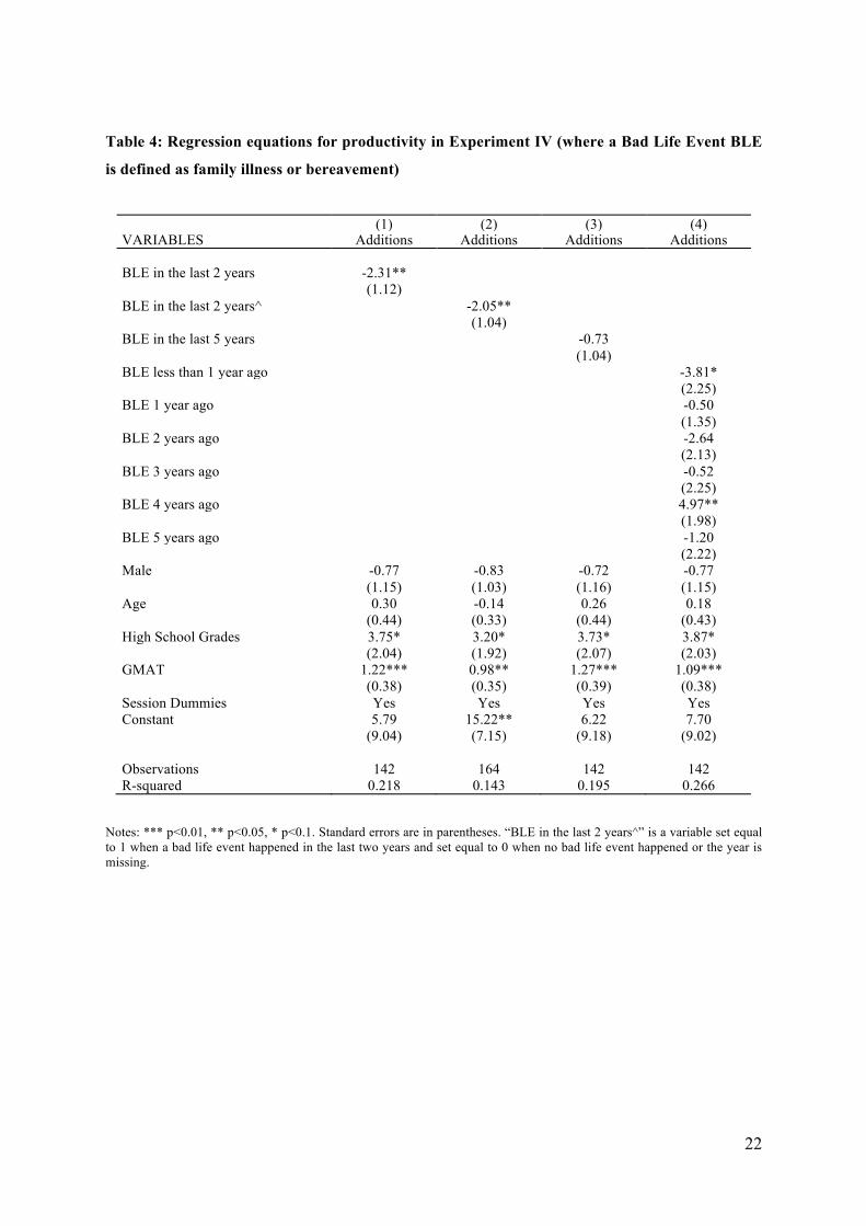
In the empirical work, we define a bad life event (BLE) to be either bereavement or illness in the
family.16 The data suggested that it was appropriate to aggregate these happiness-shock events by
using a single variable, BLE. There were 8 sessions across two days. The appendix summarizes the
means and standard deviations of the variables.
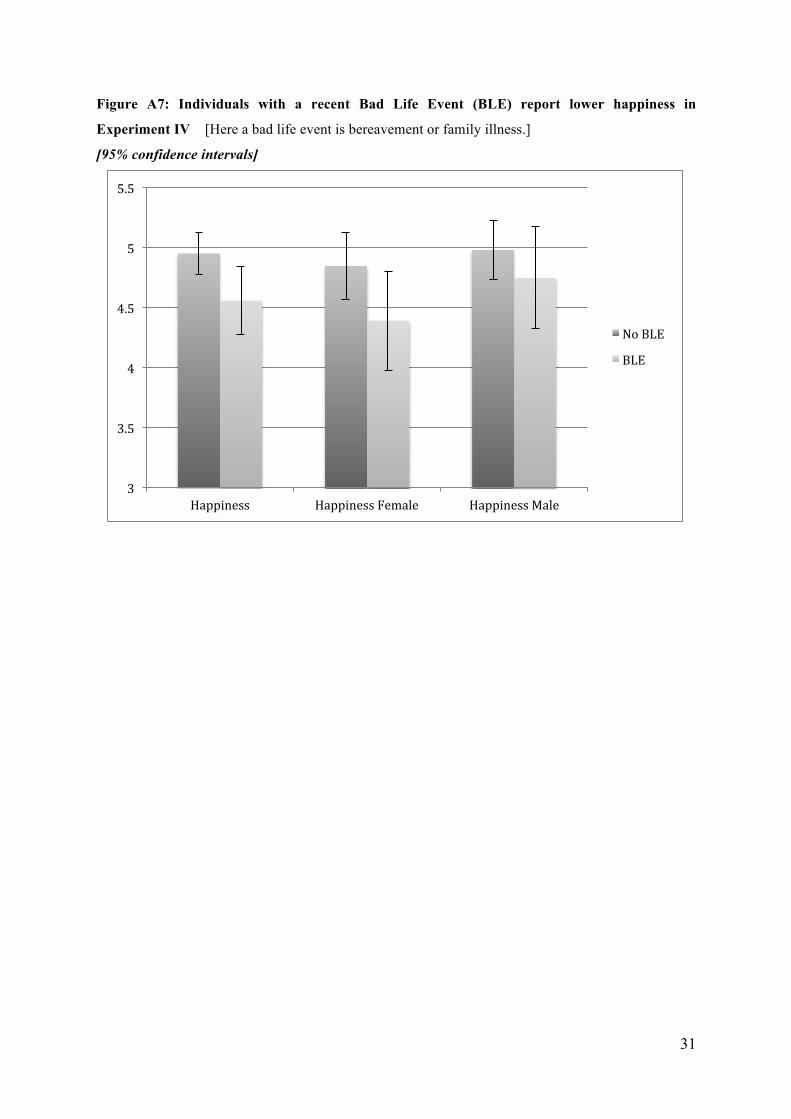
In Experiment IV, we can think of Nature as allocating extreme ‘unhappiness’ shocks. The sample
size here is 179; the mean of productivity in the sample is 18.40 with a standard deviation of 6.71.
Those subjects who have recently been through a bad life event are noticeably less happy and less
productive. Compared to the control group, they mark themselves nearly half a point lower on the
happiness scale, and they achieve approximately 2 fewer correct additions. They also make fewer
attempts. These are noticeable differences when compared to individuals in the no-BLE group. The
effects are statistically significant in the full samples; they are also statistically significant in the
majority of the subsamples. In column 1 of Table 4, for example, the productivity difference is 2.31
additions with a standard error of 1.12. On closer inspection (not reported here), it is not possible to
reject the null hypothesis that the effects are of the same size for males and females. The regression
equations in Table 4 and Table 5 illustrate what happens when a variety of covariates are included.
They also illustrate one notable result. Consistent with the idea of slow ‘hedonic adaptation’, the
family tragedies that happened longer ago seem to have smaller consequences for people’s current
happiness and productivity.
It is possible to think of some important potential objections to Experiment IV. A natural one is
16 In the questionnaire, we also asked about parental divorce; but this turned out to have a tiny (occasionally positive) and statistically insignificant effect on the individual, so the divorce of parents, at least in our data set, does not appear to qualify as a bad life event.
12
that the happiness shock is assigned by Nature rather than us. This means that it is not necessarily
randomly distributed across the sample. For example, those families most prone to bad life shocks
such as bereavement could, in principle, also be ones where unhappiness is intrinsically more
common and where productivity is intrinsically lower. This criticism is perhaps likely to have less
force among a group of elite students than in a general cross-section of the population, but it is
nevertheless a potential weakness of Experiment IV. Hence the association in the data could be real
in a statistical sense but illusory in a causal sense. A second difficulty is that it is not possible in
Experiment IV to be certain that lower happiness causes the lower productivity. Both might be
triggered by the existence of the Bad Life Event. A third difficulty is that, strictly speaking,
Experiment IV demonstrates that unhappiness is associated with lower productivity in the additions
task. It does not show the reverse, namely, that a boost to happiness promotes a boost in productivity.
In Tables 4 and 5, the regression equations for Experiment IV provide information about,
respectively, the statistical impact of a BLE bad life event in each year from year 0 to year 5 (as
declared at the end of the experiment) upon both individuals’ productivities and those individuals’
levels of happiness (as declared at the beginning of the experiment). At -0.55 in the upper left-hand
column of Table 5, the immediate estimate on well-being is large and negative. In column 4 of Table
5, the immediate-run loss of happiness is apparently even greater, at approximately one full point.
Therefore, although our subjects may not be aware of it, their happiness answers at the start of
Experiment IV are correlated with whether later on they report that a BLE recently occurred in their
family. The pattern in the happiness coefficients is itself broadly consistent with hedonic adaptation -
- the well-being effect declines through time. Overall, the consequence of a bad life event is
empirically strong if it happened less than a year ago, and becomes insignificantly different from zero
after approximately 3 years. Our results are consistent with a range of adaptation findings in the
survey-based research literature on the economics of human well-being (e.g. Clark et al. 2008).
We are especially interested in the effects of a bad life event upon human performance. The
regressions in Table 4 provide a range of estimates of the impact of BLE on productivity. Having
had a bad event in the previous year is associated with particularly low performance on the additions
task. Across the columns, the size of the productivity effect is large; it is typically more than two
additions and thus greater than 10%. The extent of the deleterious effect of a Bad Life Event upon
subjects’ productivity is a declining function of the elapsed time since the event. This finding may
repay scrutiny in future empirical research.
3. Conclusions
This study provides evidence of a link between human happiness and human productivity. To our
knowledge, it is the first such evidence -- though we would like to acknowledge the work of the late
Alice Isen within the field of psychology -- in a true piece-rate setting. Our study is also the first to
13
exploit information on tragic family life events as a ‘natural’ experiment and to gather within-person
information in a longitudinal way.
Four kinds of trial (denoted Experiments I to IV) have been described. The last of these is an
attempt to estimate the repercussions of life-events assigned by Nature. The design, in that case, has
the disadvantage that we cannot directly control the happiness shock, but it has the advantage that it
allows us to study large shocks -- ones that no social-science funding body would allow us to impose
on laboratory subjects -- of a fundamental kind in real human beings’ lives. The other three
experiments examine the consequences of truly randomly-assigned happiness. These experiments
have the advantage that we can directly control the happiness shock but the disadvantage that shocks
are inevitably small and of a special kind in the laboratory. It is conceivable in the last experiment
that there is some unobservable feature of people that makes them both less productive and more
likely to report a bad life event. Yet such a mechanism cannot explain the results in the other three
experiments. By design, the four Experiments I, II, III, and IV have complementary strengths and
weaknesses.
We have not, within this research project, attempted to discriminate between different theoretical
explanations for our key result. That will eventually require a different form of inquiry. Tsai et al.
(2007) and Hermalin and Isen (2008) discuss potential pathways, and the results of Killingsworth and
Gilbert (2010) suggest the possibility that unhappiness may lead to a lack of mental concentration. 17
A related possible mechanism is sketched in the appendix: it is a model of ‘worrying’ and distraction.
It is consistent with ideas in sources such as Benjamin et al. (2012) and Mani et al. (2013). One
possibility is thus that background unhappiness acts to distract rationally-optimizing individuals away
from their work tasks. 18
Various implications emerge from the experimental results. First, it appears that economists and
other social scientists may need to pay more attention to emotional well-being as a causal force.
Second, better bridges may be required between currently disparate scholarly disciplines. Third, if
happiness in a workplace carries with it a return in productivity, the paper’s findings may have
consequences for firms’ promotion policies19, and may be relevant for managers and human resources
specialists. Finally, if well-being boosts people’s performance at work, this raises the possibility, at
the microeconomic level and perhaps even the macroeconomic level, of self-sustaining spirals
between human productivity and human well-being.
17 One approach, as in Hermalin and Isen (2008), is to allow a general dynamic utility function where good mood is an argument in the utility function, and that mood can, in principle, affect the marginal rate of substitution between other elements in the utility function. 18 See the model in the appendix. 19 Over and above so-called neoclassical pay-effort mechanisms discussed in sources such as Lazear (1981) and Oswald (1984).
14
References
Amabile, Teresa M., Barsade, Sigal G., Mueller, Jennifer S., and Staw, Barry M. 2005. Affect and
creativity at work. Administrative Science Quarterly 50: 367-403.
Argyle, Michael. 1989. Do happy workers work harder? The effect of job satisfaction on job
performance. In: Ruut Veenhoven (ed), How harmful is happiness? Consequences of enjoying
life or not, Universitaire Pers Rotterdam, The Netherlands.
Ashby, F. Gregory, Isen, Alice M., and Turken, And U. 1999. A neuropsychological theory of
positive affect and its influence on cognition. Psychological Review 106: 529-550.
Baker, S.C., Frith, Christopher D., and Dolan, Raymond J. 1997. The interaction between mood and
cognitive function studied with PET. Psychological Medicine 27: 565-578.
Banerjee, Abhijit, and Mullainathan, Sendhil. 2008. Limited attention and income distribution.
Working paper. MIT.
Benabou, Roland, and Tirole, Jean. 2003. Intrinsic and extrinsic motivation. Review of Economic
Studies 70: 489-520.
Benjamin Daniel, Heffetz, Ori, Kimball, Miles S., and Rees-Jones, Alex. 2012. What do you think
would make you happier? What do you think you would choose? American Economic Review,
102(5): 2083–2110.
Bennedsen, Morten, Perez-Gonzalez, Francisco, and Wolfenzon, Daniel. 2010. Do CEOs matter?
Working paper, Stanford GSB.
Bewley, Truman. Why wages don’t fall in a recession. Harvard University Press, Cambridge. 1999.
Blanchflower, David G., and Oswald, Andrew J. 2004. Well-being over time in Britain and the USA.
Journal of Public Economics 88: 1359-1386.
Bockerman, Petri, and Ilmakunnas, Pekka. 2012. The job satisfaction-productivity nexus: A study
using matched survey and register data. Industrial and Labor Relations Review 65: 244-262.
Caves, Richard E. 1974. Multinational firms, competition, and productivity in host-country markets.
Economica 41: 176-193.
Clark, Andrew E., Diener, Edward, Georgellis, Yannis, and Lucas, Richard E. 2008. Lags and leads in
life satisfaction: A test of the baseline hypothesis. Economic Journal 118: F222-F243.
Compte, Olivier, and Postlewaite, Andrew. 2004. Confidence-enhanced performance. American
Economic Review 94: 1536-1557.
De Neve, Jan-Emmanuel, and Oswald, Andrew J. 2012. Estimating the influence of life satisfaction
and positive affect on later income using sibling fixed effects. Proceedings of the National
Academy of Sciences of the United States of America 109: 19953-19958.
Dickinson, David L. 1999. An experimental examination of labor supply and work intensities.
Journal of Labor Economics 17, 638-670.
15
Diener, Edward, Suh, Eunkook M., Lucas, Richard E., and Smith, Heidi L. 1999. Subjective well-
being: Three decades of progress. Psychological Bulletin 125(2): 276-302.
Di Tella, Rafael, MacCulloch, Robert J., and Oswald, Andrew J. 2001. Preferences over inflation and
unemployment: Evidence from surveys of happiness. American Economic Review 91, 335-341.
Easterlin, Richard A. 2003. Explaining happiness. Proceedings of the National Academy of Sciences
100: 11176-11183.
Edmans, Alex. 2012. The link between job satisfaction and firm value, with implications for corporate
social responsibility. Academy of Management Perspectives 26: 1-19.
Erez, Amir, and Isen, Alice M. 2002. The influence of positive affect on the components of
expectancy motivation. Journal of Applied Psychology 89: 1055–1067.
Estrada, Carlos A., Isen, Alice M., and Young, Mark J. 1997. Positive affect facilitates integration of
information and decreases anchoring in reasoning among physicians. Organizational Behavior
and Human Decision Processes 72: 117–135.
Forgas, Joseph P. 1989. Mood effects on decision making strategies. Australian Journal of
Psychology 41: 197–214.
Frederickson, Barbara L., and Joiner, Thomas. 2002. Positive emotions trigger upward spirals toward
emotional well-being. Psychological Science 13: 172–175.
Freeman, Richard B. 1978. Job satisfaction as an economic variable. American Economic Review, 68,
135-141.
Frey, Bruno S., and Stutzer, Alois. 2002. Happiness and Economics. Princeton, USA.
Gneezy, Uri, and Rustichini, Aldo. 2000. Pay enough or don't pay at all, Quarterly Journal of
Economics 115: 791-810.
Hermalin, Benjamin E., and Isen, Alice M. 2008. A model of the effect of affect on economic
decision-making. Quantitative Marketing and Economics 6: 17-40.
Ichniowski, Casey, and Shaw, Kathryn. 1999. The effects of human resource management systems on
economic performance: An international comparison of US and Japanese plants. Management
Science 45: 704-721.
Ifcher, John, and Zarghamee, Homa. 2011. Happiness and time preference: The effect of positive
affect in a random-assignment experiment. American Economic Review: 101(7), 3109-3129.
Isen, Alice M. 2000. Positive affect and decision making. In M. Lewis & J. M. Haviland (Eds.),
Handbook of emotions. 2nd ed. New York: The Guilford Press.
Isen, Alice M., and Reeve, Johnmarshall. 2005. The influence of positive affect on intrinsic and
extrinisic motivation: Facilitating enjoyment of play, responsible work behavior, and self-
control. Motivation and Emotion 29: 297–325.
Jundt, Dustin, and Hinsz, Verlin B. 2001. Are happier workers more productive workers? The impact
of mood on self--set goals, self--efficacy, and task performance. Paper presented at the annual
meeting of the Midwestern Psychological Association, Chicago.
16
Kavanagh, David J. 1987. Mood, persistence, and success. Australian Journal of Psychology 39: 307–
318.
Killingsworth, Matthew A., and Gilbert, Daniel T. 2010. A wandering mind is an unhappy mind.
Science 330: 932-932.
Kimball, Miles S., and Willis, Robert J. 2006. Happiness and utility. Working paper, University of
Michigan.
Kirchsteiger, Georg, Rigotti, Luca, and Rustichini, Aldo. 2006. Your morals might be your moods.
Journal of Economic Behavior and Organization 59: 155-172.
Lazear, Edward. 1981. Agency, earnings profiles, productivity, and hours restrictions. American
Economic Review 71: 606-620.
Luttmer, Erzo F.P. 2005. Neighbors as negatives: Relative earnings and well-being. Quarterly
Journal of Economics 120: 963-1002.
Layard, Richard. 2006. Happiness: Lessons from a New Science. Penguin Books, London.
Lyubomirsky, Sonja., King, Laura, and Diener, Edward. 2005. The benefits of frequent positive
affect: Does happiness lead to success? Psychological Bulletin 131, 803-855.
Mani, Anandi, Mullainathan, Sendhil, Shafir, Eldar, and Zhao, Jiaying Y. 2013. Poverty impedes
cognitive function. Science 341: 976-980.
Melton, R. Jeffrey. 1995. The role of positive affect in syllogism performance. Personality and Social
Psychology Bulletin 21: 788–794.
Niederle, Muriel, and Vesterlund, Lisa. 2007. Do women shy away from competition? Do men
compete too much? Quarterly Journal of Economics 122: 1067-1101.
Oswald, Andrew J. 1984. Wage and employment structure in an economy with internal labor markets.
Quarterly Journal of Economics 99: 693-716.
Oswald, Andrew J., and Wu, Steve. 2010. Objective confirmation of subjective measures of human
well-being: Evidence from the USA. Science 327: 576-579.
Powdthavee, Nattavudh. 2010. The Happiness Equation: The Surprising Economics of Our Most
Valuable Asset. Icon Books, London.
Patterson, Michael, Warr, Peter, and West, Michael. 2004. Organizational climate and company
productivity: The role of employee affect and employee level. Journal of Occupational and
Organizational Psychology 77: 193-216.
Pugno, Maurizio, and Depedri, Sara 2009. Job performance and job satisfaction: An integrated
survey. Working paper, Universita’ di Trento.
Sanna, Lawrence J., Turley, Kandi J., and Mark, Melvin M. 1996. Expected evaluation, goals, and
performance: Mood as input. Personality and Social Psychology Bulletin 22: 323-325.
Segal, Carmit. 2012. Working when no-one is watching: Motivation, test scores, and economic
success. Management Science 58: 1438-1457.
17
Senik, Claudia. 2004. When information dominates comparison: Learning from Russian subjective
data. Journal of Public Economics 88: 2099-2123.
Siebert, Stanley W., and Zubanov, Nikolay. 2010. Management economics in a large retail company.
Management Science 56: 1398-1414.
Sinclair, Robert C., and Mark, Melvin M. 1995. The effects of mood state on judgmental accuracy:
Processing strategy as a mechanism. Cognition and Emotion 9: 417–438.
Steele, Claude M., and Aronson, Joshua. 1995. Stereotype threat and the intellectual test performance
of African-Americans. Journal of Personality and Social Psychology 69: 797-811.
Tsai, Wei-Chi., Chen, Chien-Cheng, and Liu, Hui-Lu. 2007. Test of a model linking employee
positive moods and task performance. Journal of Applied Psychology 92: 1570-1583.
Van Praag, Bernard, and Ferrer-I-Carbonell, Ada. 2004. Happiness Quantified: A Satisfaction
Calculus Approach, Oxford University Press, Oxford.
Winkelmann, Lilliana, and Winkelmann, Rainer. 1998. Why are the unemployed so unhappy?
Evidence from panel data. Economica 65: 1-15.
Wright, Thomas A., and Staw, Barry A. 1998. Affect and favorable work outcomes: two longitudinal
tests of the happy-productive worker thesis. Journal of Organizational Behavior 20: 1-23.
Zelenski, John M., Murphy, Stephen A., and Jenkins, David A. 2008. The happy-productive worker
thesis revisited. Journal of Happiness Studies 9: 521-537.

18
TABLES
19
Table 1: Regression equations for productivity in Experiment I
(1) (2) (3) VARIABLES Additions Additions Attempts Treatment Dummy 2.11** 1.41* 1.69** (0.85) (0.83) (0.82) Explicit Payment 2.71** 2.85** (1.24) (1.22) Placebo Clip 0.012 0.45 (1.66) (1.63) Male 1.58* 1.35 (0.85) (0.84) High School Grades 7.82*** 7.78*** (1.64) (1.61) GMAT 1.33*** 1.37*** (0.31) (0.31) Session 2 0.63 1.10 (1.37) (1.35) Session 3 2.20 3.00** (1.36) (1.34) Session 4 1.12 2.34* (1.32) (1.30) Constant 16.3*** 6.06*** 8.66*** (0.61) (1.56) (1.54) Observations 276 269 269 R-squared 0.022 0.248 0.258
Notes: Productivity -- here and in later tables -- is the number of correct numerical additions done in a timed task. For completeness, the third column also reports an equation for the number of attempted answers (some of these answers may have been wrong).
*** p<0.01, ** p<0.05, * p<0.1. Standard errors are in parentheses.
20
Table 2: Regression equations for productivity in Experiment II
(1) (2) (3) (4) VARIABLES Additions
OLS
Additions
OLS
Attempts
OLS
Additions
IV
Treatment Dummy 4.15** 5.01*** 4.47*** (1.71) (1.68) (1.69) Change in Happiness 8.92** (3.70) Happiness Before 1.63 (1.56) Male 4.08** 5.64*** 2.12 (1.68) (1.69) (2.15) Age 0.16 0.19 -0.048 (0.26) (0.26) (0.33) High School Marks 3.37 3.65 4.23 (3.26) (3.28) (4.17) GMAT 2.25** 2.09** 2.89** (0.88) (0.89) (1.12) Day Dummy 1.99 0.79 1.09 (1.76) (1.77) (2.25) Constant 18.8*** 0.75 3.96 -1.67
Observations 104 100 100 100 R-squared 0.054 0.213 0.219
Notes: *** p<0.01, ** p<0.05, * p<0.1. Standard errors are in parentheses.
The change in happiness is that between the start of Experiment IV and the middle of that experiment (that is, after the happiness treatment but before the additions productivity task). It is instrumented here with a treatment 1-0 dummy variable. The treatment is exposure to the comedy clip. The control individuals watch the placebo film. The first-stage equation for the instrumented equation in column 4 can be found in Table A5 of the appendix.
21
Table 3: Regression equations for productivity in Experiment III
(1) (2) (3) VARIABLES Additions Additions Attempts
Treatment Dummy 3.07** 3.78*** 4.22*** (1.43) (1.42) (1.38) Male 2.95* 3.49** (1.49) (1.45) Age 0.18 0.16 (0.12) (0.11) High School Grades 6.33** 5.54* (3.12) (3.03) GMAT 0.73 0.78 (0.52) (0.51) Day Dummy No Yes Yes Constant 19.6*** 8.27** 12.0*** (1.01) (4.09) (3.97) Observations 148 145 145 R-squared 0.031 0.122 0.145
*** p<0.01, ** p<0.05, * p<0.1. Standard errors are in parentheses.
22
Table 4: Regression equations for productivity in Experiment IV (where a Bad Life Event BLE
is defined as family illness or bereavement)
(1) (2) (3) (4) VARIABLES Additions Additions Additions Additions BLE in the last 2 years -2.31** (1.12) BLE in the last 2 years^ -2.05** (1.04) BLE in the last 5 years -0.73 (1.04) BLE less than 1 year ago -3.81* (2.25) BLE 1 year ago -0.50 (1.35) BLE 2 years ago -2.64 (2.13) BLE 3 years ago -0.52 (2.25) BLE 4 years ago 4.97** (1.98) BLE 5 years ago -1.20 (2.22) Male -0.77 -0.83 -0.72 -0.77 (1.15) (1.03) (1.16) (1.15) Age 0.30 -0.14 0.26 0.18 (0.44) (0.33) (0.44) (0.43) High School Grades 3.75* 3.20* 3.73* 3.87* (2.04) (1.92) (2.07) (2.03) GMAT 1.22*** 0.98** 1.27*** 1.09*** (0.38) (0.35) (0.39) (0.38) Session Dummies Yes Yes Yes Yes
Constant 5.79 15.22** 6.22 7.70 (9.04) (7.15) (9.18) (9.02) Observations 142 164 142 142 R-squared 0.218 0.143 0.195 0.266
Notes: *** p<0.01, ** p<0.05, * p<0.1. Standard errors are in parentheses. “BLE in the last 2 years^” is a variable set equal to 1 when a bad life event happened in the last two years and set equal to 0 when no bad life event happened or the year is missing.
23
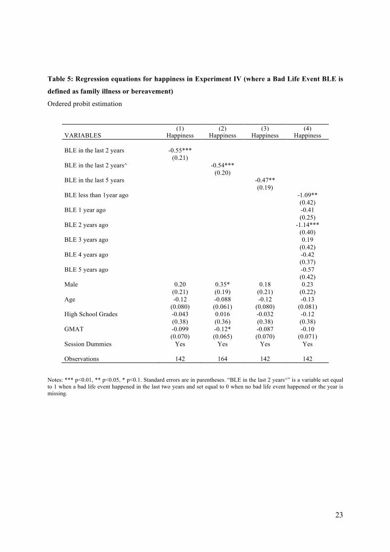
Table 5: Regression equations for happiness in Experiment IV (where a Bad Life Event BLE is
defined as family illness or bereavement)
Ordered probit estimation
(1) (2) (3) (4) VARIABLES Happiness Happiness Happiness Happiness BLE in the last 2 years -0.55*** (0.21) BLE in the last 2 years^ -0.54*** (0.20) BLE in the last 5 years -0.47** (0.19) BLE less than 1year ago -1.09** (0.42) BLE 1 year ago -0.41 (0.25) BLE 2 years ago -1.14*** (0.40) BLE 3 years ago 0.19 (0.42) BLE 4 years ago -0.42 (0.37) BLE 5 years ago -0.57 (0.42) Male 0.20 0.35* 0.18 0.23 (0.21) (0.19) (0.21) (0.22) Age -0.12 -0.088 -0.12 -0.13 (0.080) (0.061) (0.080) (0.081) High School Grades -0.043 0.016 -0.032 -0.12 (0.38) (0.36) (0.38) (0.38) GMAT -0.099 -0.12* -0.087 -0.10 (0.070) (0.065) (0.070) (0.071) Session Dummies Yes Yes Yes Yes Observations 142 164 142 142
Notes: *** p<0.01, ** p<0.05, * p<0.1. Standard errors are in parentheses. “BLE in the last 2 years^” is a variable set equal to 1 when a bad life event happened in the last two years and set equal to 0 when no bad life event happened or the year is missing.

24
APPENDIX: Part 1
25
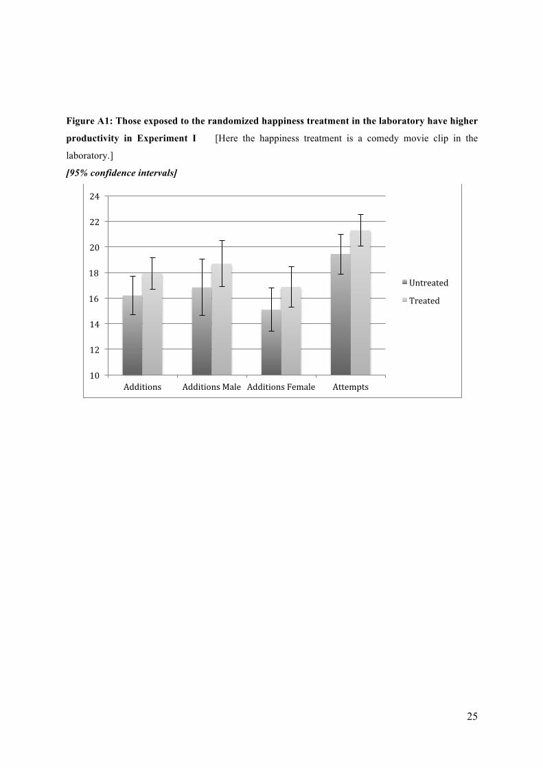
Figure A1: Those exposed to the randomized happiness treatment in the laboratory have higher
productivity in Experiment I [Here the happiness treatment is a comedy movie clip in the
laboratory.]
[95% confidence intervals]
10
12
14
16
18
20
22
24
Additions Additions Male Additions Female Attempts
Untreated
Treated
26
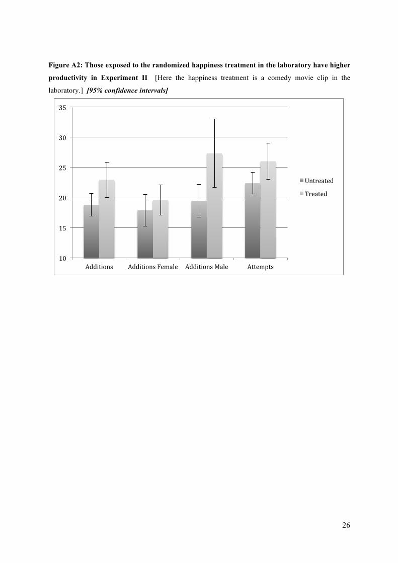
Figure A2: Those exposed to the randomized happiness treatment in the laboratory have higher
productivity in Experiment II [Here the happiness treatment is a comedy movie clip in the
laboratory.] [95% confidence intervals]
10
15
20
25
30
35
Additions Additions Female Additions Male Attempts
Untreated
Treated
27
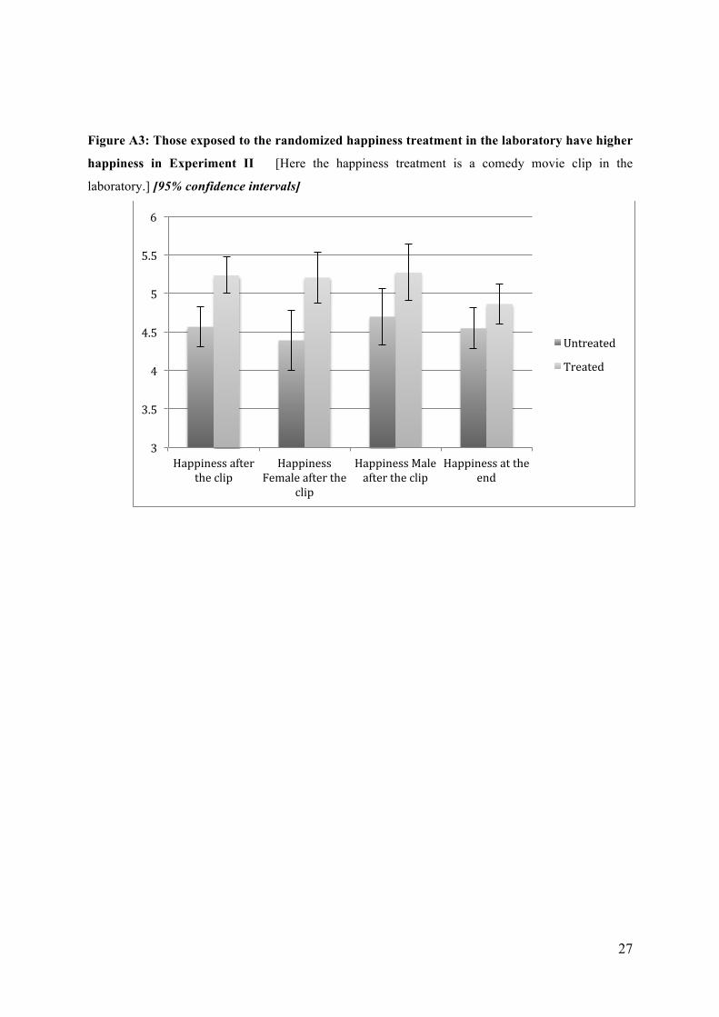
Figure A3: Those exposed to the randomized happiness treatment in the laboratory have higher
happiness in Experiment II [Here the happiness treatment is a comedy movie clip in the
laboratory.] [95% confidence intervals]
3
3.5
4
4.5
5
5.5
6
Happiness after the clip
Happiness Female after the
clip
Happiness Male after the clip
Happiness at the end
Untreated
Treated
28
Figure A4: Those exposed to the randomized happiness treatment in the laboratory have higher
productivity in Experiment III [Here the happiness treatment is chocolates+fruit+drinks in the
laboratory.] [95% confidence intervals]
10
15
20
25
30
Additions Additions Female Additions Male Attempts
Untreated
Treated
29
Figure A5: Correlational evidence (non-causal) that the greatest rise in happiness during
Experiment II is associated with the greatest productivity gain [Here those not exposed to the
happiness treatment have the same baseline productivity; hence the y axis can be viewed as a change
in productivity from the common baseline.]
020
4060
80
-4 -2 0 2Happiness at the end - Happiness before clip
95% CI Fitted valuesCorrect Additions
30
Figure A6: Individuals with a recent Bad Life Event (BLE) have lower productivity in
Experiment IV [Here a bad life event is bereavement or family illness.]
[95% confidence intervals]
10
12
14
16
18
20
22
24
26
Additions Additions Female Additions Male Attempts
No BLE
BLE
31
Figure A7: Individuals with a recent Bad Life Event (BLE) report lower happiness in
Experiment IV [Here a bad life event is bereavement or family illness.]
[95% confidence intervals]
3
3.5
4
4.5
5
5.5
Happiness Happiness Female Happiness Male
No BLE
BLE
32
APPENDIX: Part 2 The purpose of this appendix is to give more details on the data, and provide some robustness checks
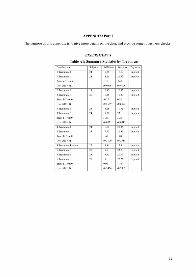
EXPERIMENT I
Table A1: Summary Statistics by Treatment Day\Session Subjects Additions Attempts Payment
1 Treatment 0 24 15.38 17.67 Implicit
1 Treatment 1 24 18.21 21.33 Implicit
Treat 1-Treat 0 1.18 3.66
(Ha: diff > 0) (0.0476) (0.0126)
2 Treatment 0 23 16.85 20.92 Implicit
2 Treatment 1 20 16.48 19.39 Implicit
Treat 1-Treat 0 -0.37 0.81
(Ha: diff > 0) (0.5669) (0.6393)
3 Treatment 0 23 16.26 19.73 Implicit
3 Treatment 1 24 19.52 23 Implicit
Treat 1-Treat 0 3.26 3.26
(Ha: diff > 0) (0.0521) (0.0513)
4 Treatment 0 24 16.04 20.36 Implicit
4 Treatment 1 25 17.72 21.45 Implicit
Treat 1-Treat 0 1.68 1.09
(Ha: diff > 0) (0.3109) (0.3018)
5 Treatment Placebo 25 14.84 17.8 Implicit
5 Treatment 1 25 19.8 23.8 Explicit
6 Treatment 0 23 18.52 20.90 Explicit
6 Treatment 1 21 19 22.26 Explicit
Treat 1-Treat 0 0.90 1.78
(Ha: diff > 0) (0.3426) (0.2003)
33
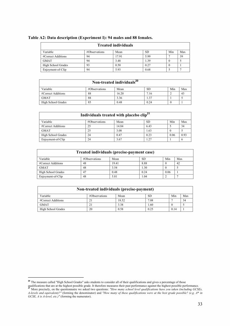
Table A2: Data description (Experiment I): 94 males and 88 females.
Treated individuals
Variable #Observations Mean SD Min Max #Correct Additions 94 17.91 5.99 7 39 GMAT 94 3.48 1.39 0 5 High School Grades 93 0.50 0.27 0 1 Enjoyment-of-Clip 94 5.93 0.68 5 7
Non-treated individuals20
Variable #Observations Mean SD Min Max #Correct Additions 88 16.20 7.16 2 43 GMAT 88 3.36 1.37 1 5 High School Grades 85 0.48 0.24 0 1
Individuals treated with placebo clip21
Variable #Observations Mean SD Min Max #Correct Additions 25 14.84 6.43 5 34 GMAT 25 3.08 1.63 0 5 High School Grades 24 0.47 0.23 0.06 0.93 Enjoyment-of-Clip 24 3.67 1.27 1 6
Treated individuals (precise-payment case)
Variable #Observations Mean SD Min Max #Correct Additions 48 19.41 8.88 0 42 GMAT 48 3.54 1.30 0 5 High School Grades 47 0.48 0.24 0.06 1 Enjoyment-of-Clip 48 5.81 1.04 2 7
Non-treated individuals (precise-payment)
Variable #Observations Mean SD Min Max #Correct Additions 21 18.52 7.08 7 34 GMAT 21 3.38 1.60 0 5 High School Grades 20 0.58 0.25 0.14 1
20 The measure called "High School Grades" asks students to consider all of their qualifications and gives a percentage of those qualifications that are at the highest possible grade. It therefore measures their past performance against the highest possible performance. 21 More precisely, on the questionnaire we asked two questions: "How many school level qualifications have you taken (including GCSEs, A-levels and equivalent)?" (forming the denominator) and "How many of these qualifications were at the best grade possible? (e.g. A* in GCSE, A is A-level, etc.)" (forming the numerator).
34
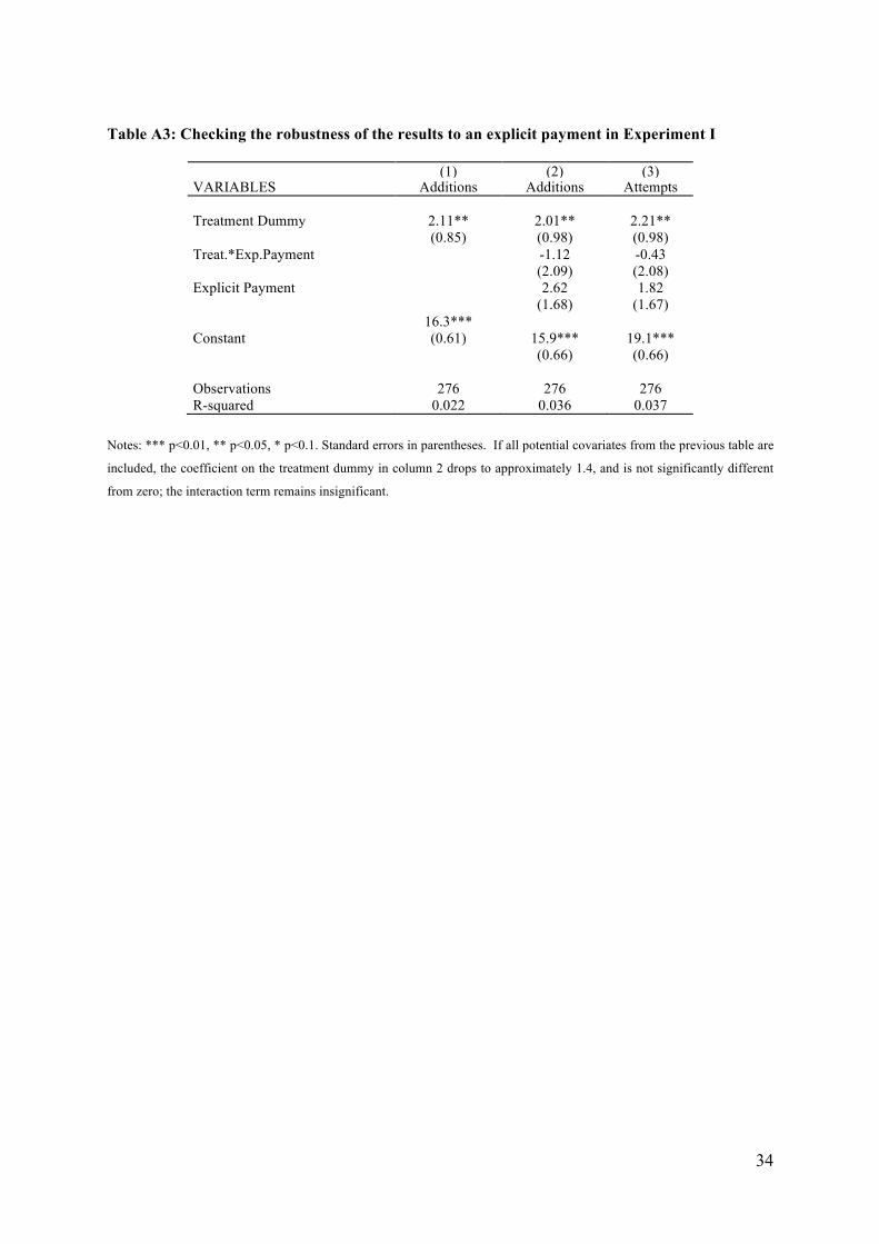
Table A3: Checking the robustness of the results to an explicit payment in Experiment I
(1) (2) (3) VARIABLES Additions Additions Attempts
Treatment Dummy 2.11** 2.01** 2.21** (0.85) (0.98) (0.98) Treat.*Exp.Payment -1.12 -0.43 (2.09) (2.08) Explicit Payment 2.62 1.82
(1.68) (1.67)
16.3*** Constant (0.61) 15.9*** 19.1*** (0.66) (0.66) Observations 276 276 276 R-squared 0.022 0.036 0.037
Notes: *** p<0.01, ** p<0.05, * p<0.1. Standard errors in parentheses. If all potential covariates from the previous table are
included, the coefficient on the treatment dummy in column 2 drops to approximately 1.4, and is not significantly different
from zero; the interaction term remains insignificant.
35
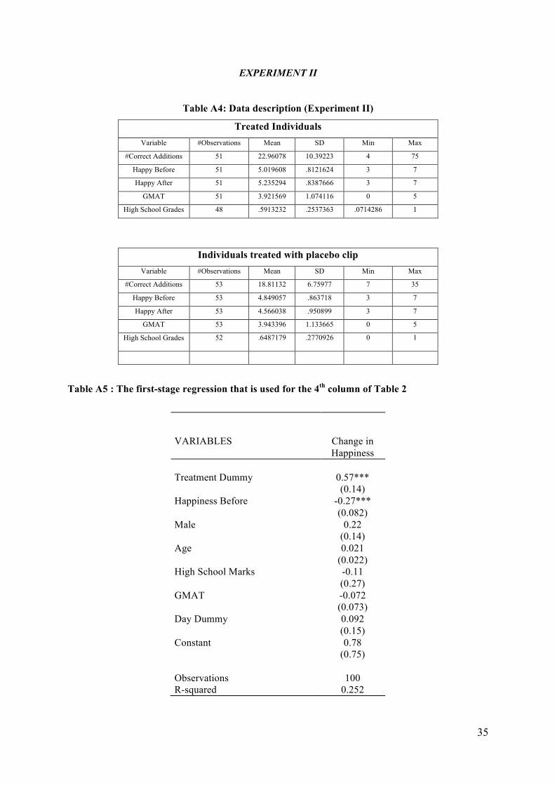
EXPERIMENT II
Table A4: Data description (Experiment II)
Treated Individuals Variable #Observations Mean SD Min Max
#Correct Additions 51 22.96078 10.39223 4 75
Happy Before 51 5.019608 .8121624 3 7
Happy After 51 5.235294 .8387666 3 7
GMAT 51 3.921569 1.074116 0 5
High School Grades 48 .5913232 .2537363 .0714286 1
Individuals treated with placebo clip Variable #Observations Mean SD Min Max
#Correct Additions 53 18.81132 6.75977 7 35
Happy Before 53 4.849057 .863718 3 7
Happy After 53 4.566038 .950899 3 7
GMAT 53 3.943396 1.133665 0 5
High School Grades 52 .6487179 .2770926 0 1
Table A5 : The first-stage regression that is used for the 4th column of Table 2
VARIABLES Change in Happiness
Treatment Dummy 0.57*** (0.14) Happiness Before -0.27*** (0.082) Male 0.22 (0.14) Age 0.021 (0.022) High School Marks -0.11 (0.27) GMAT -0.072 (0.073) Day Dummy 0.092 (0.15) Constant 0.78 (0.75) Observations 100 R-squared 0.252
36
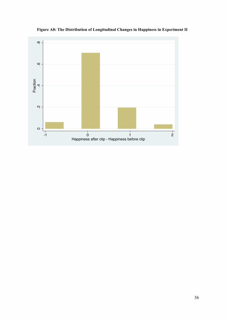
Figure A8: The Distribution of Longitudinal Changes in Happiness in Experiment II
0.2
.4.6
.8Fr
actio
n
-1 0 1 2Happiness after clip - Happiness before clip
37
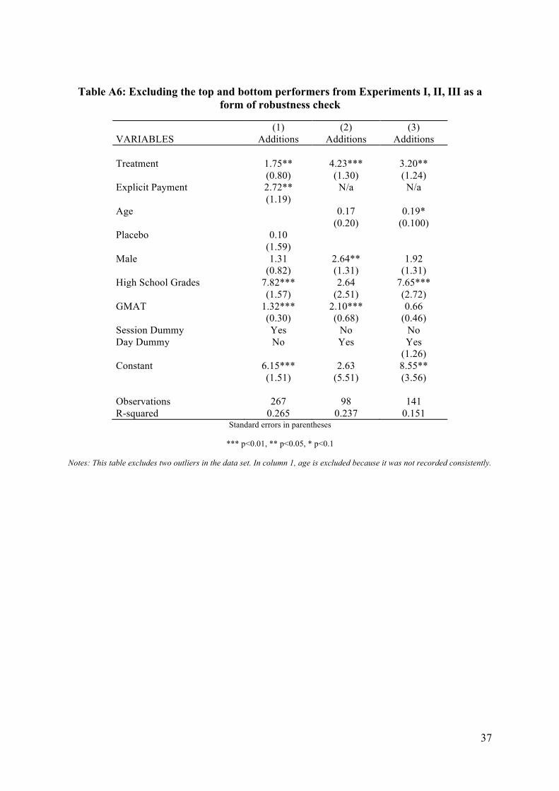
Table A6: Excluding the top and bottom performers from Experiments I, II, III as a form of robustness check
(1) (2) (3) VARIABLES Additions Additions Additions Treatment 1.75** 4.23*** 3.20** (0.80) (1.30) (1.24) Explicit Payment 2.72** N/a N/a (1.19) Age 0.17 0.19* (0.20) (0.100) Placebo 0.10 (1.59) Male 1.31 2.64** 1.92 (0.82) (1.31) (1.31) High School Grades 7.82*** 2.64 7.65*** (1.57) (2.51) (2.72) GMAT 1.32*** 2.10*** 0.66 (0.30) (0.68) (0.46) Session Dummy Yes No No Day Dummy No Yes Yes (1.26) Constant 6.15*** 2.63 8.55** (1.51) (5.51) (3.56) Observations 267 98 141 R-squared 0.265 0.237 0.151
Standard errors in parentheses
*** p<0.01, ** p<0.05, * p<0.1
Notes: This table excludes two outliers in the data set. In column 1, age is excluded because it was not recorded consistently.
38
EXPERIMENT III
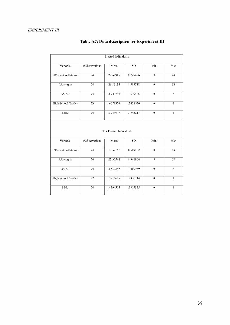
Table A7: Data description for Experiment III
Treated Individuals
Variable #Observations Mean SD Min Max
#Correct Additions 74 22.68919 8.747486 8 49
#Attempts 74 26.35135 8.503718 9 56
GMAT 74 3.783784 1.519465 0 5
High School Grades 73 .4679374 .2438676 0 1
Male 74 .5945946 .4943217 0 1
Non Treated Individuals
Variable #Observations Mean SD Min Max
#Correct Additions 74 19.62162 8.589102 0 49
#Attempts 74 22.90541 8.361964 5 50
GMAT 74 3.837838 1.489939 0 5
High School Grades 72 .5210657 .2310314 0 1
Male 74 .4594595 .5017555 0 1
39
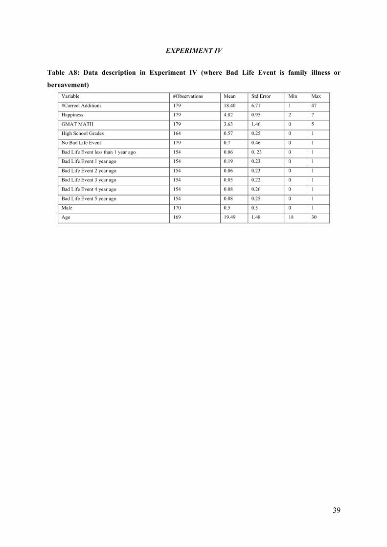
EXPERIMENT IV
Table A8: Data description in Experiment IV (where Bad Life Event is family illness or
bereavement) Variable #Observations Mean Std Error Min Max
#Correct Additions 179 18.40 6.71 1 47
Happiness 179 4.82 0.95 2 7
GMAT MATH 179 3.63 1.46 0 5
High School Grades 164 0.57 0.25 0 1
No Bad Life Event 179 0.7 0.46 0 1
Bad Life Event less than 1 year ago 154 0.06 0. 23 0 1
Bad Life Event 1 year ago 154 0.19 0.23 0 1
Bad Life Event 2 year ago 154 0.06 0.23 0 1
Bad Life Event 3 year ago 154 0.05 0.22 0 1
Bad Life Event 4 year ago 154 0.08 0.26 0 1
Bad Life Event 5 year ago 154 0.08 0.25 0 1
Male 170 0.5 0.5 0 1
Age 169 19.49 1.48 18 30
40
APPENDIX: Part 3
A Potential Microeconomic Theory of Distracted Worrying
Consider the following model22. Its main result stems from internal resource-allocation by
the worker. In the model, a positive happiness shock, h, allows the employee to devote more attention
and effort to solving problems at work (essentially because the worker can switch from worrying).
Let the worker be uncertain about his or her randomly distributed ability, z. This has a density
function f(z). Denote p as the piece-rate level of pay. Let e be the effort the employee devotes to
solving tasks at work. Let w be the effort the worker devotes to ‘worrying’ about other things.
Define R as the worker’s psychological resources. Assume (e + w) has to be less than or equal to R.
Let u be the utility from working. It depends on income and effort.
Let v be the utility from worrying (that is, from being distracted). Worrying can be thought of as
rational concern for issues in the worker’s life that need his or her attention. In a paid-task setting, it
might be stress about the possibility of failure at the task. But, more broadly, it can be any general
form of distraction from the job at hand. For human beings, it might be plausible to think of a worker
as alternating, during the day, between concentrating on the task and feeling anxious about his or her
life.
Assume there is an initial happiness shock, h. Define overall utility as u+v.
People therefore solve the problem: Choose work-effort e to
Maximize ∫ + ),()(),,,( hwvdzzfzhepu
subject to weR +≥ .
The first-order condition for a maximum in this problem is
0=− we vEu . (1)
The comparative-static result of particular interest is the response of productivity, given by work
effort e, to a rise in the initial happiness shock, h.
22 Although we proposed this in the first 2008 draft of the current paper, the approach has much in common with the independently developed, and much more empirically supported, important ideas of Benjamin et al. 2012. Mani et al. (2013) contains related ideas.
41
It is determined in a standard way. The sign of de*/dh takes the sign of the cross partial of
the maximand, namely:
Sign de*/dh takes the sign of wheh vEu + . (2)
Without more restrictions, this sign could be positive or negative. The happiness shock could
increase or decrease productivity in the work task.
However, to get some insight into the likely outcome, consider simple forms of the utility
functions, and assume that workers know their own productivity, so are not subject to the uncertainty,
and that R is normalized to unity. Set z to unity for simplicity.
Assume u and v are both concave functions.
An additively separable case
Assume additive separability. Then, assuming the worker gets the h happiness shock whether she
subsequently works or worries, the worker solves
Maximize hevpeu 2)1()( +−+ (3)
and hence at an interior maximum
0)1()( =−ʹ′−ʹ′ evppeu (4)
so here the optimal work effort e* is independent of the happiness shock, h.
Another concavity case
A more plausible form of utility function has the happiness shock within a concave form.
Here the worker solves
Maximize )1()( hevhpeu +−++
which is the assumption that h is a shift variable within the utility function itself, rather than an
additive part of that function.
Now the first-order condition is
0)1()( =+−ʹ′−+ʹ′ hevphpeu . (5)
Here the optimal level of energy devoted to solving problems at work, e*, does depend on the level of
the happiness shock, h.
42
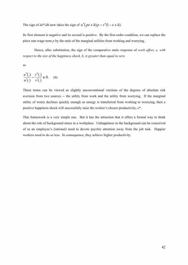
The sign of de*/dh now takes the sign of )1()( hevphpeu +−ʹ′ʹ′−+ʹ′ʹ′ .
Its first element is negative and its second is positive. By the first-order condition, we can replace the
piece rate wage term p by the ratio of the marginal utilities from working and worrying.
Hence, after substitution, the sign of the comparative static response of work effort, e, with
respect to the size of the happiness shock, h, is greater than equal to zero
as
.0(.)(.)
(.)(.)
≥ʹ′
ʹ′ʹ′−
ʹ′
ʹ′ʹ′
vv
uu
(6)
These terms can be viewed as slightly unconventional versions of the degrees of absolute risk
aversion from two sources -- the utility from work and the utility from worrying. If the marginal
utility of worry declines quickly enough as energy is transferred from working to worrying, then a
positive happiness shock will successfully raise the worker’s chosen productivity, e*.
This framework is a very simple one. But it has the attraction that it offers a formal way to think
about the role of background stress in a workplace. Unhappiness in the background can be conceived
of as an employee’s (rational) need to devote psychic attention away from the job task. Happier
workers need to do so less. In consequence, they achieve higher productivity.