1

Paper 5760-2016

Hands-on GTL

Kriss Harris, SAS Specialists Limited

ABSTRACT

Would you like to be more confident in producing graphs and figures? Do you understand the differences between the OVERLAY, GRIDDED, LATTICE, DATAPANEL, and DATALATTICE layouts? Would you like to know how to easily create life sciences industry standard graphs such as adverse event timelines, Kaplan-Meier plots, and waterfall plots? Finally, would you like to learn all these methods in a relaxed environment that fosters questions? Great—this topic is for you! In this hands-on workshop, you will be guided through the Graph Template Language (GTL). You will also complete fun and challenging SAS graphics exercises to enable you to more easily retain what you have learned. This session is structured so that you will learn how to create the standard plots that your manager requests, how to easily create simple ad hoc plots for your customers, and also how to create complex graphics. You will be shown different methods to annotate your plots, including how to add Unicode characters to your plots. You will find out how to create reusable templates, which can be used by your team. Years of information have been carefully condensed into this 90-minute hands-on, highly interactive session. Feel free to bring some of your challenging graphical questions along!

INTRODUCTION

GTL can be used to create sophisticated graphs. Some graphs cannot be created with SGPLOT, SGPANEL or SGSCATTER but can be created with GTL. Examples of these are trellised graphs with independent axes, and multiple-cell graphs with different cell proportions, and multiple-cell graphs with different plot types, i.e. one cell is a bar chart, and another is a box plot. With GTL you can also produce reproducible templates.

According to (Matange, Getting Started with the Graph Template Language in SAS: Examples, Tips, and Techniques for Creating Custom Graphs, 2013, p. 5) here are some reasons to learn GTL.

GTL provides in one system the full set of features that you need to create graphs from the simplest scatter plots to complex diagnostics panels.

GTL is the language used to create the templates shipped by SAS for the creation of the automatic graphs from the analytical procedures. To customize one of these graphs, you will need to understand GTL.

GTL represents the future for analytical graphics in SAS. New features are being added to GTL with every SAS release.

This paper intends to motivate you to use GTL, to introduce you to GTL, to show you how you can create plots in GTL which cannot be produced with the SG Procedures, and to show you how to create reusable templates. SAS

® 9.4 was used to run the code in this paper.

The dataset used in this paper is from the CDISC SDTM / ADAM Pilot Project and this was obtained from the CDISC website (CDISC, 2013).

FROM SG PROCEDURES TO GTL

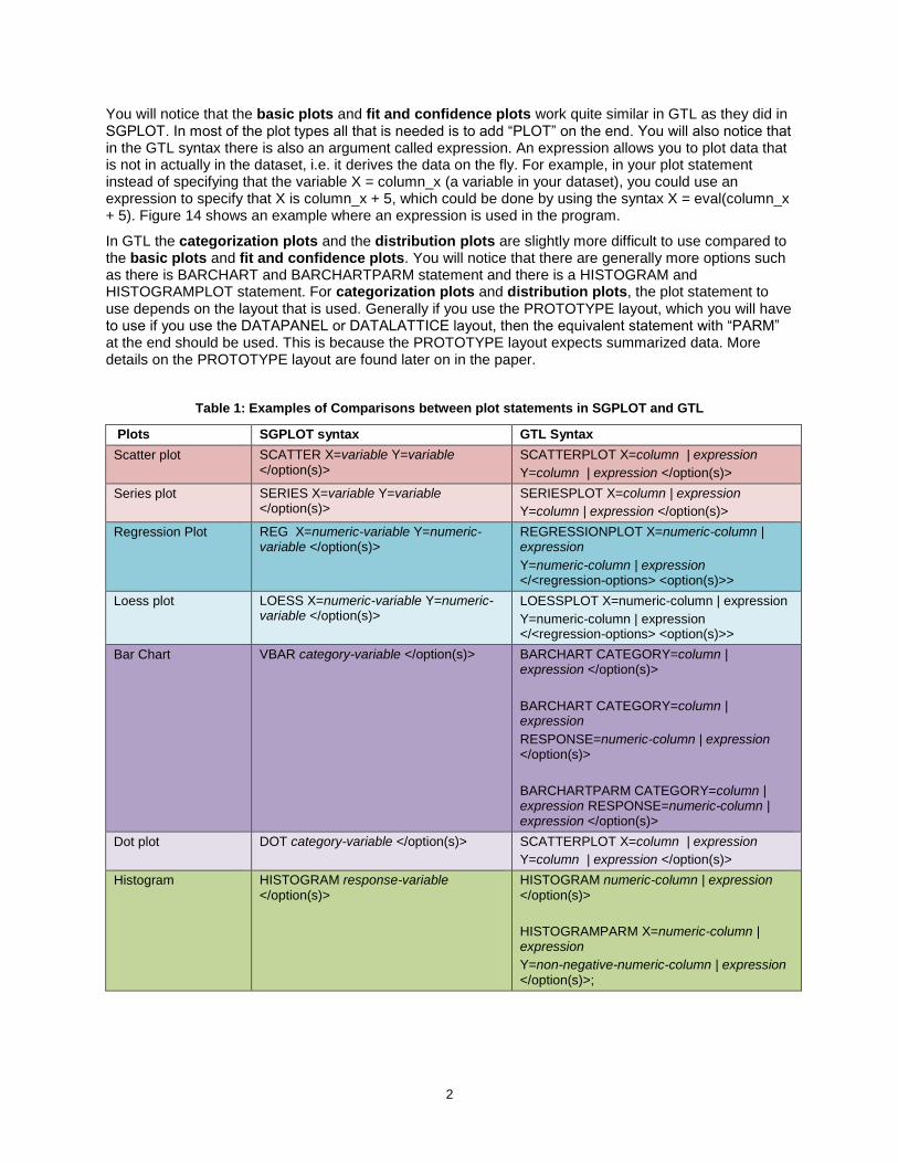
If you are familiar with SGPLOT then you will probably find it easier to understand the GTL syntax. Literally it is like learning a new language! Table 1 below shows the relationships in the syntax between SGPLOT and GTL in the plot statements and Table 2 shows options that you are most likely to use. The general background color of Table 1 represents the plot type that the plot would be in SGPLOT. In this context the general background color means that the red and pink color are both referred to as red, and similar groupings are done with the other colors. The red background represents the basic plots type, aqua represents fit and confidence plots, purple represents the categorization plots, and olive green represents the distribution plots.

2

You will notice that the basic plots and fit and confidence plots work quite similar in GTL as they did in SGPLOT. In most of the plot types all that is needed is to add “PLOT” on the end. You will also notice that in the GTL syntax there is also an argument called expression. An expression allows you to plot data that is not in actually in the dataset, i.e. it derives the data on the fly. For example, in your plot statement instead of specifying that the variable X = column_x (a variable in your dataset), you could use an expression to specify that X is column_x + 5, which could be done by using the syntax X = eval(column_x + 5). Figure 14 shows an example where an expression is used in the program.

In GTL the categorization plots and the distribution plots are slightly more difficult to use compared to the basic plots and fit and confidence plots. You will notice that there are generally more options such as there is BARCHART and BARCHARTPARM statement and there is a HISTOGRAM and HISTOGRAMPLOT statement. For categorization plots and distribution plots, the plot statement to use depends on the layout that is used. Generally if you use the PROTOTYPE layout, which you will have to use if you use the DATAPANEL or DATALATTICE layout, then the equivalent statement with “PARM” at the end should be used. This is because the PROTOTYPE layout expects summarized data. More details on the PROTOTYPE layout are found later on in the paper.

Table 1: Examples of Comparisons between plot statements in SGPLOT and GTL

Plots SGPLOT syntax GTL Syntax

Scatter plot SCATTER X=variable Y=variable </option(s)>

SCATTERPLOT X=column | expression

Y=column | expression </option(s)>

Series plot SERIES X=variable Y=variable </option(s)>

SERIESPLOT X=column | expression

Y=column | expression </option(s)>

Regression Plot REG X=numeric-variable Y=numeric-variable </option(s)>

REGRESSIONPLOT X=numeric-column | expression

Y=numeric-column | expression </<regression-options> <option(s)>>

Loess plot LOESS X=numeric-variable Y=numeric-variable </option(s)>

LOESSPLOT X=numeric-column | expression

Y=numeric-column | expression </<regression-options> <option(s)>>

Bar Chart VBAR category-variable </option(s)> BARCHART CATEGORY=column | expression </option(s)>

BARCHART CATEGORY=column | expression

RESPONSE=numeric-column | expression </option(s)>

BARCHARTPARM CATEGORY=column | expression RESPONSE=numeric-column | expression </option(s)>

Dot plot DOT category-variable </option(s)> SCATTERPLOT X=column | expression

Y=column | expression </option(s)>

Histogram HISTOGRAM response-variable </option(s)>

HISTOGRAM numeric-column | expression </option(s)>

HISTOGRAMPARM X=numeric-column | expression

Y=non-negative-numeric-column | expression </option(s)>;

3

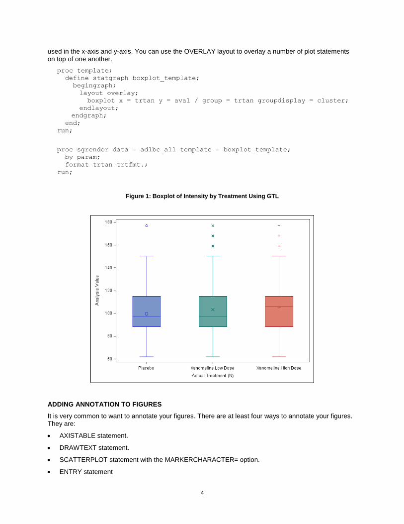
Plots SGPLOT syntax GTL Syntax

Boxplots VBOX analysis-variable </option(s)> BOXPLOT Y=numeric-column | expression </option(s)>

BOXPLOT X=column | expression

Y=numeric-column | expression </option(s)>

BOXPLOTPARM Y=numeric-column | expression

STAT=string-column </option(s)>

BOXPLOTPARM X=column | expression

Y=numeric-column | expression

STAT=string-column </option(s)>

Table 2: Examples of Comparisons between option in SGPLOT and GTL

Options SGPLOT syntax GTL Syntax

Change x-axis label XAXIS label = "New Label"; XAXISOPTS=(label = "New Label")

Change y-axis range YAXIS min = 0 max = 0; YAXISOPTS=(linearopts=(viewmin=0 viewmax=100))

Specify tick values YAXIS values=(0 to 100 by 10); YAXISOPTS=(linearopts=(tickvaluesequence=(start=0 end=0 increment=10)))

CREATING A GRAPH USING GTL

As explained in (McConville & Much, 2015), in GTL, graphs are built by using plot and layout statements. The plot statements determine how data are represented in the graph, and the layout statements determine where the plots are drawn on the graph. More advanced layouts can be used to divide the plot area into multiple independent cells. In addition, statements can be nested so multiple plots can be arranged to create elegant visuals.

As mentioned in (Matange, Getting Started with the Graph Template Language in SAS: Examples, Tips, and Techniques for Creating Custom Graphs, 2013), creating a graph using GTL is a two-step process, which uses both the TEMPLATE and SGRENDER procedures.

Firstly, you define the structure of the graph in the form of the STATGRAPH template using GTL. The typical syntax is shown below.

proc template;

define statgraph <template-name>;

begingraph / <options>;

<GTL statements>;

endgraph;

end;

run;

Secondly, you associate the data with the template using the SGRENDER procedure to create the graph.

proc sgrender data=<data-set-name> template=<template-name>;

<other optional statements>;

run;

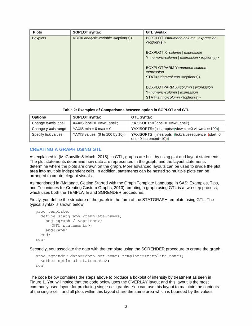
The code below combines the steps above to produce a boxplot of intensity by treatment as seen in Figure 1. You will notice that the code below uses the OVERLAY layout and this layout is the most commonly used layout for producing single-cell graphs. You can use this layout to maintain the contents of the single-cell, and all plots within this layout share the same area which is bounded by the values

4

used in the x-axis and y-axis. You can use the OVERLAY layout to overlay a number of plot statements on top of one another.

proc template;

define statgraph boxplot_template;

begingraph;

layout overlay;

boxplot x = trtan y = aval / group = trtan groupdisplay = cluster;

endlayout;

endgraph;

end;

run;

proc sgrender data = adlbc_all template = boxplot_template;

by param;

format trtan trtfmt.;

run;

Figure 1: Boxplot of Intensity by Treatment Using GTL

ADDING ANNOTATION TO FIGURES

It is very common to want to annotate your figures. There are at least four ways to annotate your figures. They are:

AXISTABLE statement.

DRAWTEXT statement.

SCATTERPLOT statement with the MARKERCHARACTER= option.

ENTRY statement

5

This paper shows examples of the first two options: AXISTABLE and DRAWTEXT. To add summary statistics and align the summary statistics with the values on the xaxis, you can use AXISTABLE. This can be seen in Figure 2.

proc template;

define statgraph boxplot_template;

begingraph;

layout overlay;

boxplot x = trtan y = aval / group = trtan groupdisplay = cluster;

innermargin / align=bottom opaque=true;

axistable x = trtan value = bigN / stat=mean label = "N";

axistable x = trtan value = mean / stat=mean label = "Mean";

axistable x = trtan value = stddev / stat=mean label = "SD";

endinnermargin;

endlayout;

endgraph;

end;

run;

Figure 2: Using AXISTABLE to show Summary Statistics

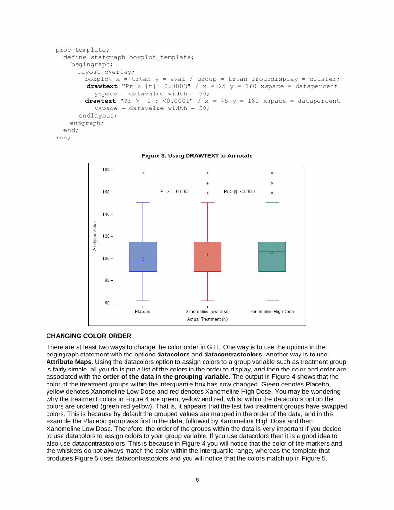
If you want to add text anywhere on your graph you can use the DRAWTEXT statement. This is useful because it is extremely flexible in terms of placing text anywhere on your graph, e.g. placing text beside the Boxplots and/or beside the x-axis label. Placement of the text is controlled by the x and y values and also the options that are selected for the xspace and yspace. Figure 3 shows a Boxplot of Intensity by Treatment with p-values of the treatment different that were added using the DRAWTEXT statement. For more information on this type of annotation please see (Matange, Annotate your SGPLOT Graphs, 2014).

6

proc template;

define statgraph boxplot_template;

begingraph;

layout overlay;

boxplot x = trtan y = aval / group = trtan groupdisplay = cluster;

drawtext "Pr > |t|: 0.0003" / x = 25 y = 160 xspace = datapercent

yspace = datavalue width = 30;

drawtext "Pr > |t|: <0.0001" / x = 75 y = 160 xspace = datapercent

yspace = datavalue width = 30;

endlayout;

endgraph;

end;

run;

Figure 3: Using DRAWTEXT to Annotate

CHANGING COLOR ORDER

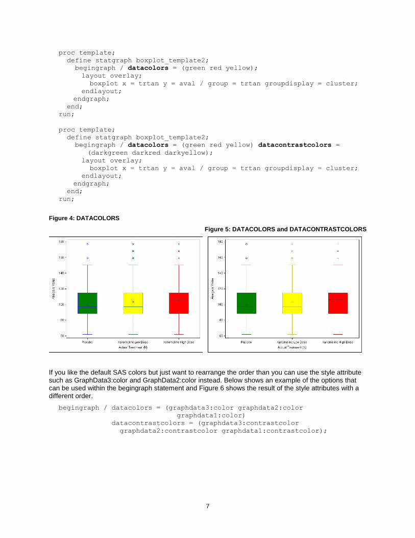
There are at least two ways to change the color order in GTL. One way is to use the options in the begingraph statement with the options datacolors and datacontrastcolors. Another way is to use Attribute Maps. Using the datacolors option to assign colors to a group variable such as treatment group is fairly simple, all you do is put a list of the colors in the order to display, and then the color and order are associated with the order of the data in the grouping variable. The output in Figure 4 shows that the color of the treatment groups within the interquartile box has now changed. Green denotes Placebo, yellow denotes Xanomeline Low Dose and red denotes Xanomeline High Dose. You may be wondering why the treatment colors in Figure 4 are green, yellow and red, whilst within the datacolors option the colors are ordered (green red yellow). That is, it appears that the last two treatment groups have swapped colors. This is because by default the grouped values are mapped in the order of the data, and in this example the Placebo group was first in the data, followed by Xanomeline High Dose and then Xanomeline Low Dose. Therefore, the order of the groups within the data is very important if you decide to use datacolors to assign colors to your group variable. If you use datacolors then it is a good idea to also use datacontrastcolors. This is because in Figure 4 you will notice that the color of the markers and the whiskers do not always match the color within the interquartile range, whereas the template that produces Figure 5 uses datacontrastcolors and you will notice that the colors match up in Figure 5.

7

proc template;

define statgraph boxplot_template2;

begingraph / datacolors = (green red yellow);

layout overlay;

boxplot x = trtan y = aval / group = trtan groupdisplay = cluster;

endlayout;

endgraph;

end;

run;

proc template;

define statgraph boxplot_template2;

begingraph / datacolors = (green red yellow) datacontrastcolors =

(darkgreen darkred darkyellow);

layout overlay;

boxplot x = trtan y = aval / group = trtan groupdisplay = cluster;

endlayout;

endgraph;

end;

run;

Figure 4: DATACOLORS

Figure 5: DATACOLORS and DATACONTRASTCOLORS

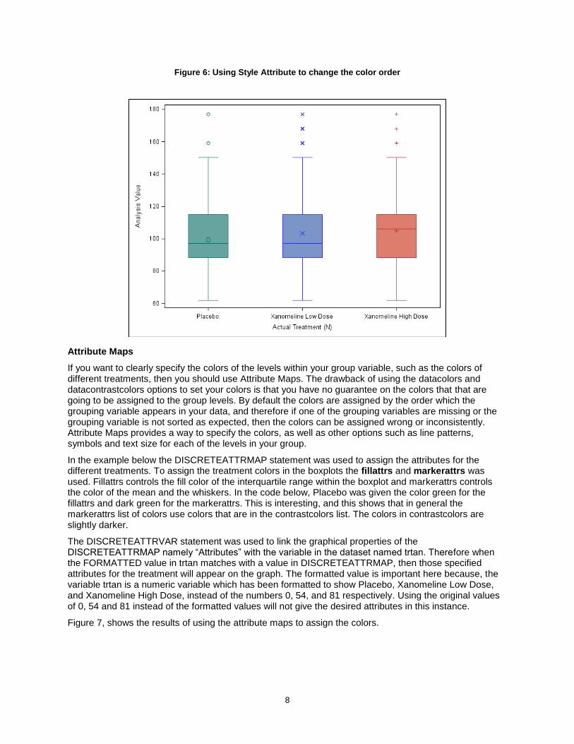
If you like the default SAS colors but just want to rearrange the order than you can use the style attribute such as GraphData3:color and GraphData2:color instead. Below shows an example of the options that can be used within the begingraph statement and Figure 6 shows the result of the style attributes with a different order.

begingraph / datacolors = (graphdata3:color graphdata2:color

graphdata1:color)

datacontrastcolors = (graphdata3:contrastcolor

graphdata2:contrastcolor graphdata1:contrastcolor);

8

Figure 6: Using Style Attribute to change the color order

Attribute Maps

If you want to clearly specify the colors of the levels within your group variable, such as the colors of different treatments, then you should use Attribute Maps. The drawback of using the datacolors and datacontrastcolors options to set your colors is that you have no guarantee on the colors that that are going to be assigned to the group levels. By default the colors are assigned by the order which the grouping variable appears in your data, and therefore if one of the grouping variables are missing or the grouping variable is not sorted as expected, then the colors can be assigned wrong or inconsistently. Attribute Maps provides a way to specify the colors, as well as other options such as line patterns, symbols and text size for each of the levels in your group.

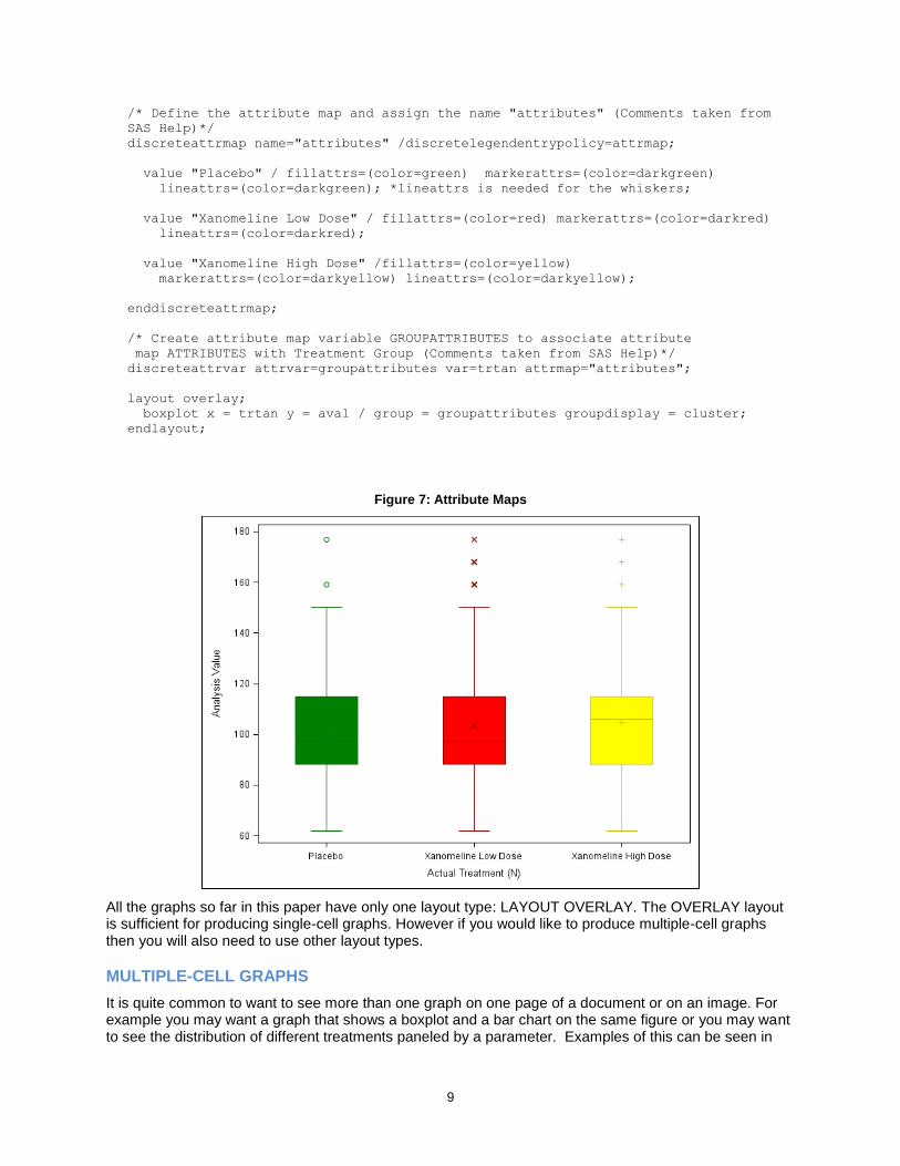
In the example below the DISCRETEATTRMAP statement was used to assign the attributes for the different treatments. To assign the treatment colors in the boxplots the fillattrs and markerattrs was used. Fillattrs controls the fill color of the interquartile range within the boxplot and markerattrs controls the color of the mean and the whiskers. In the code below, Placebo was given the color green for the fillattrs and dark green for the markerattrs. This is interesting, and this shows that in general the markerattrs list of colors use colors that are in the contrastcolors list. The colors in contrastcolors are slightly darker.

The DISCRETEATTRVAR statement was used to link the graphical properties of the DISCRETEATTRMAP namely “Attributes” with the variable in the dataset named trtan. Therefore when the FORMATTED value in trtan matches with a value in DISCRETEATTRMAP, then those specified attributes for the treatment will appear on the graph. The formatted value is important here because, the variable trtan is a numeric variable which has been formatted to show Placebo, Xanomeline Low Dose, and Xanomeline High Dose, instead of the numbers 0, 54, and 81 respectively. Using the original values of 0, 54 and 81 instead of the formatted values will not give the desired attributes in this instance.

Figure 7, shows the results of using the attribute maps to assign the colors.

9

/* Define the attribute map and assign the name "attributes" (Comments taken from

SAS Help)*/

discreteattrmap name="attributes" /discretelegendentrypolicy=attrmap;

value "Placebo" / fillattrs=(color=green) markerattrs=(color=darkgreen)

lineattrs=(color=darkgreen); *lineattrs is needed for the whiskers;

value "Xanomeline Low Dose" / fillattrs=(color=red) markerattrs=(color=darkred)

lineattrs=(color=darkred);

value "Xanomeline High Dose" /fillattrs=(color=yellow)

markerattrs=(color=darkyellow) lineattrs=(color=darkyellow);

enddiscreteattrmap;

/* Create attribute map variable GROUPATTRIBUTES to associate attribute

map ATTRIBUTES with Treatment Group (Comments taken from SAS Help)*/

discreteattrvar attrvar=groupattributes var=trtan attrmap="attributes";

layout overlay;

boxplot x = trtan y = aval / group = groupattributes groupdisplay = cluster;

endlayout;

Figure 7: Attribute Maps

All the graphs so far in this paper have only one layout type: LAYOUT OVERLAY. The OVERLAY layout is sufficient for producing single-cell graphs. However if you would like to produce multiple-cell graphs then you will also need to use other layout types.

MULTIPLE-CELL GRAPHS

It is quite common to want to see more than one graph on one page of a document or on an image. For example you may want a graph that shows a boxplot and a bar chart on the same figure or you may want to see the distribution of different treatments paneled by a parameter. Examples of this can be seen in

10

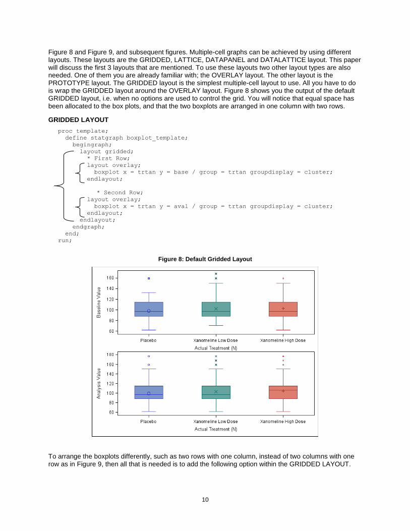
Figure 8 and Figure 9, and subsequent figures. Multiple-cell graphs can be achieved by using different layouts. These layouts are the GRIDDED, LATTICE, DATAPANEL and DATALATTICE layout. This paper will discuss the first 3 layouts that are mentioned. To use these layouts two other layout types are also needed. One of them you are already familiar with; the OVERLAY layout. The other layout is the PROTOTYPE layout. The GRIDDED layout is the simplest multiple-cell layout to use. All you have to do is wrap the GRIDDED layout around the OVERLAY layout. Figure 8 shows you the output of the default GRIDDED layout, i.e. when no options are used to control the grid. You will notice that equal space has been allocated to the box plots, and that the two boxplots are arranged in one column with two rows.

GRIDDED LAYOUT

proc template;

define statgraph boxplot_template;

begingraph;

layout gridded;

* First Row;

layout overlay;

boxplot x = trtan y = base / group = trtan groupdisplay = cluster;

endlayout;

* Second Row;

layout overlay;

boxplot x = trtan y = aval / group = trtan groupdisplay = cluster;

endlayout;

endlayout;

endgraph;

end;

run;

Figure 8: Default Gridded Layout

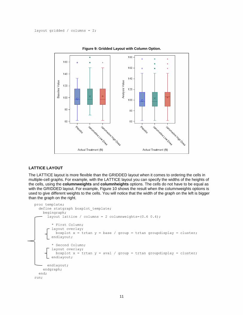
To arrange the boxplots differently, such as two rows with one column, instead of two columns with one row as in Figure 9, then all that is needed is to add the following option within the GRIDDED LAYOUT.

11

layout gridded / columns = 2;

Figure 9: Gridded Layout with Column Option.

LATTICE LAYOUT

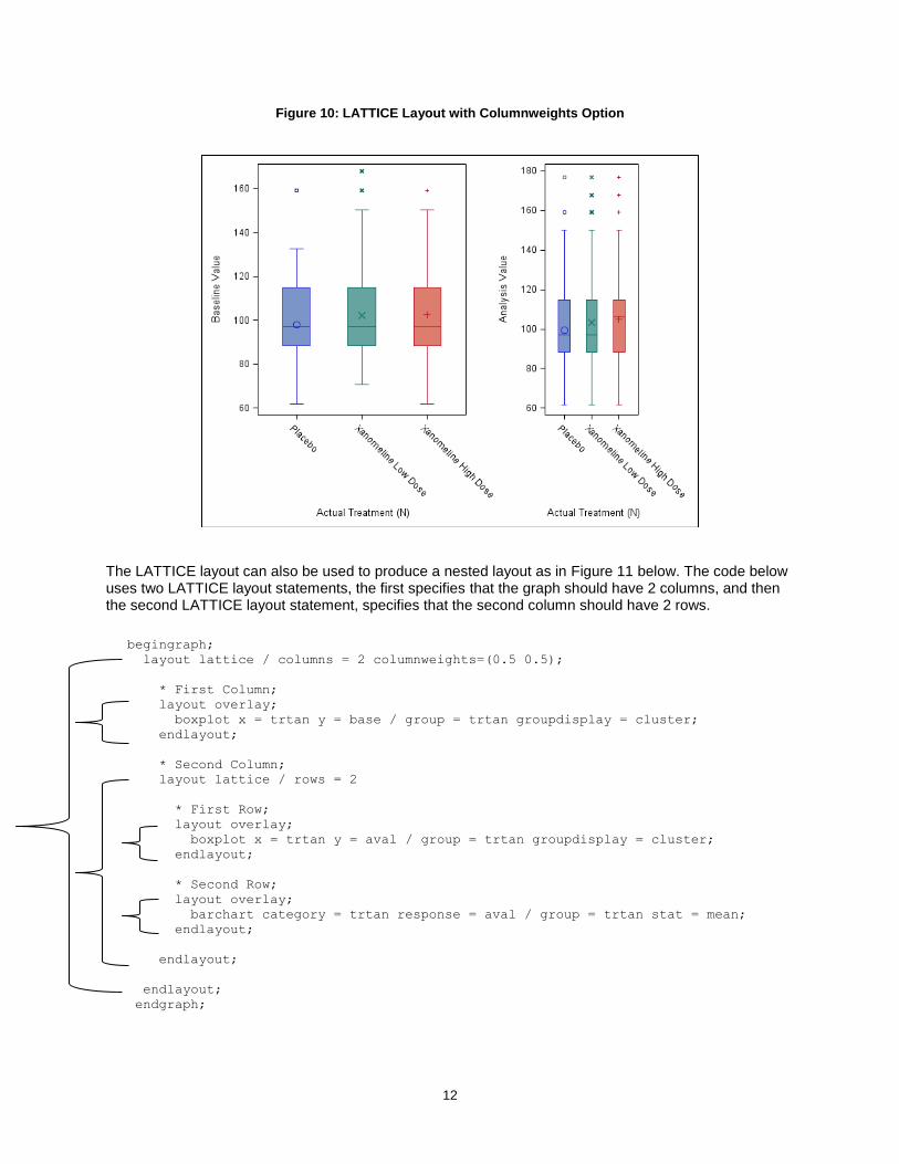
The LATTICE layout is more flexible than the GRIDDED layout when it comes to ordering the cells in multiple-cell graphs. For example, with the LATTICE layout you can specify the widths of the heights of the cells, using the columnweights and columnheights options. The cells do not have to be equal as with the GRIDDED layout. For example, Figure 10 shows the result when the columnweights options is used to give different weights to the cells. You will notice that the width of the graph on the left is bigger than the graph on the right.

proc template;

define statgraph boxplot_template;

begingraph;

layout lattice / columns = 2 columnweights=(0.6 0.4);

* First Column;

layout overlay;

boxplot x = trtan y = base / group = trtan groupdisplay = cluster;

endlayout;

* Second Column;

layout overlay;

boxplot x = trtan y = aval / group = trtan groupdisplay = cluster;

endlayout;

endlayout;

endgraph;

end;

run;

12

Figure 10: LATTICE Layout with Columnweights Option

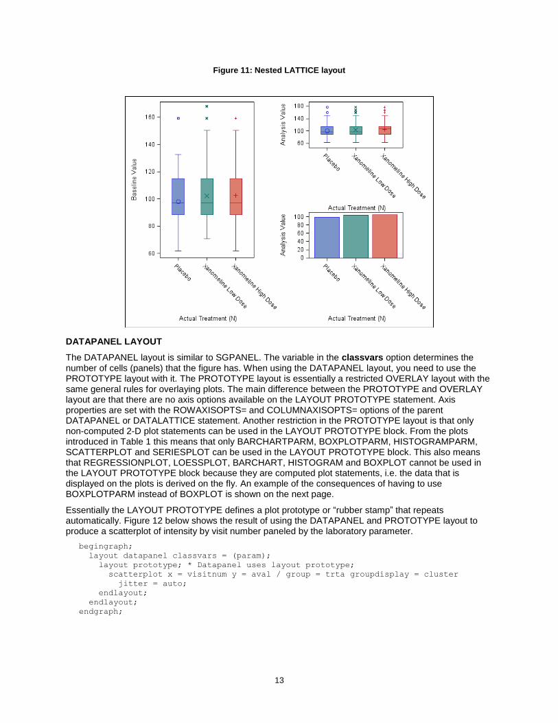
The LATTICE layout can also be used to produce a nested layout as in Figure 11 below. The code below uses two LATTICE layout statements, the first specifies that the graph should have 2 columns, and then the second LATTICE layout statement, specifies that the second column should have 2 rows.

begingraph;

layout lattice / columns = 2 columnweights=(0.5 0.5);

* First Column;

layout overlay;

boxplot x = trtan y = base / group = trtan groupdisplay = cluster;

endlayout;

* Second Column;

layout lattice / rows = 2

* First Row;

layout overlay;

boxplot x = trtan y = aval / group = trtan groupdisplay = cluster;

endlayout;

* Second Row;

layout overlay;

barchart category = trtan response = aval / group = trtan stat = mean;

endlayout;

endlayout;

endlayout;

endgraph;

13

Figure 11: Nested LATTICE layout

DATAPANEL LAYOUT

The DATAPANEL layout is similar to SGPANEL. The variable in the classvars option determines the number of cells (panels) that the figure has. When using the DATAPANEL layout, you need to use the PROTOTYPE layout with it. The PROTOTYPE layout is essentially a restricted OVERLAY layout with the same general rules for overlaying plots. The main difference between the PROTOTYPE and OVERLAY layout are that there are no axis options available on the LAYOUT PROTOTYPE statement. Axis properties are set with the ROWAXISOPTS= and COLUMNAXISOPTS= options of the parent DATAPANEL or DATALATTICE statement. Another restriction in the PROTOTYPE layout is that only non-computed 2-D plot statements can be used in the LAYOUT PROTOTYPE block. From the plots introduced in Table 1 this means that only BARCHARTPARM, BOXPLOTPARM, HISTOGRAMPARM, SCATTERPLOT and SERIESPLOT can be used in the LAYOUT PROTOTYPE block. This also means that REGRESSIONPLOT, LOESSPLOT, BARCHART, HISTOGRAM and BOXPLOT cannot be used in the LAYOUT PROTOTYPE block because they are computed plot statements, i.e. the data that is displayed on the plots is derived on the fly. An example of the consequences of having to use BOXPLOTPARM instead of BOXPLOT is shown on the next page.

Essentially the LAYOUT PROTOTYPE defines a plot prototype or “rubber stamp” that repeats automatically. Figure 12 below shows the result of using the DATAPANEL and PROTOTYPE layout to produce a scatterplot of intensity by visit number paneled by the laboratory parameter.

begingraph;

layout datapanel classvars = (param);

layout prototype; * Datapanel uses layout prototype;

scatterplot x = visitnum y = aval / group = trta groupdisplay = cluster

jitter = auto;

endlayout;

endlayout;

endgraph;

14

Figure 12: Scatterplot with DATAPANEL

In Figure 12, the y-axis ranges from 0 to 2000. From now on when discussing the DATAPANEL layout, the y-axis will be referred to as row-axis, and the x-axis will be referred to as column-axis, as this is more correct. You will notice that the range of the row-axis makes it difficult to see all the results for each laboratory parameter. Also it appears that showing the intensity values on the log scale and using a different plot such as the boxplot instead of the scatterplot might be more appropriate.

In the rowaxisopts you can set the intensity values to be on the log scale, and in the PROTOTYPE layout you can use boxplotparm to create boxplots. As mentioned above, the PROTOTYPE layout does not accept computed plot statements. Therefore you cannot use the boxplot statement; however, you can use the boxplotparm statement. Firstly the dataset needs to be manipulated so that it contains the minimum, maximum, mean, median, 1st quartile and 3rd quartile of the data that you want to plot, which in this case is by treatment and visit number. Then secondly, you plot the data that has already been summarized. In SAS help, there is a generalized macro called %boxcompute which can help you to summarize the data.

Figure 13 shows the result of using the boxplotparm and shows a boxplot of the intensity by the visit number for each treatment, paneled by the laboratory parameter. The treatment legend is produced by using the DISCRETELEGEND statement within the SIDEBAR block.

begingraph;

layout datapanel classvars = (param) / columns = 2

rowaxisopts = (type = log label = "Lab Intensity Values") rowdatarange=union;

layout prototype;

boxplotparm x = visitnum y = col1 stat = _NAME_ / group = trta groupdisplay =

cluster name = "trtleg";

endlayout;

sidebar;

discretelegend "trtleg";

endsidebar;

endlayout;

endgraph;

15

Figure 13: Boxplot with DATAPANEL

In Figure 13, you will notice that the columns have the same column-axis. In all the laboratory parameters the visit numbers range from 4 to 12. You will also notice that each row has the same row-axis. That is, the parameters, Alanine Aminotransferase (ALT) and Aspartate Aminotransferase (AST) range from approximately 1 to 160 and the parameters Creatine Kinase and Creatinine range from 10 to approximately 1000. The fact that at least the row or the column has to have the same axes makes the DATAPANEL layout very good for making comparisons between the rows or the columns or both. For example, it is very easy to notice that the variability in the Creatinine parameter is much smaller than the variability in Creatine Kinase, which is likely due to the difference in unit, and so a different axis might be better for a smaller unit.

If you were interested in looking at data with different units or seeing how the data within each parameter is distributed, so that you can assess the treatment difference, or investigate if there are any points outside the limits then you might be interested in using a layout that has the functionality for using independent axes.

Independent Axes

You can use layouts that you are already familiar with: LATTICE and OVERLAY to produce plots with independent axes. (Hebber & Matange, 2013) show how you can simulate the subsetting of observation in GTL. You can use these ideas as illustrated in the program below to create cells that have independent axes. Evidently, it is possible for you to create cells using GTL that have independent axes without simulating the subsetting of observations. However, using another method to create cells that have independent axes involves reformatting your dataset, so that there is an x-variable and a y-variable for every parameter that you want to plot. Therefore if you have lots of parameters, you will end up with a dataset with a large number of columns.

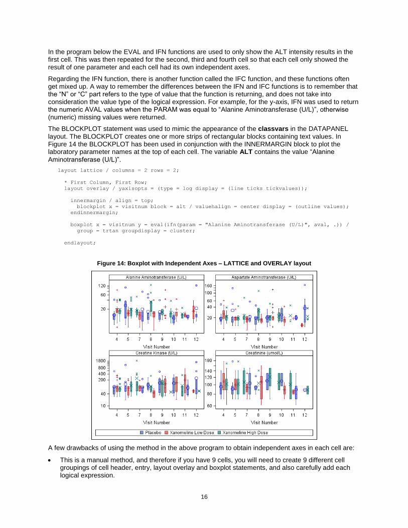
The program below shows a snippet of the full GTL code which produces the template for Figure 14. Figure 14 shows boxplots of intensity by visit number for four laboratory parameters, and each laboratory parameter has its own independent axes. Figure 14 was created using the layouts LAYOUT LATTICE and LAYOUT OVERLAY.

Same row-axis

Same row-axis

16

In the program below the EVAL and IFN functions are used to only show the ALT intensity results in the first cell. This was then repeated for the second, third and fourth cell so that each cell only showed the result of one parameter and each cell had its own independent axes.

Regarding the IFN function, there is another function called the IFC function, and these functions often get mixed up. A way to remember the differences between the IFN and IFC functions is to remember that the “N” or “C” part refers to the type of value that the function is returning, and does not take into consideration the value type of the logical expression. For example, for the y-axis, IFN was used to return the numeric AVAL values when the PARAM was equal to “Alanine Aminotransferase (U/L)”, otherwise (numeric) missing values were returned.

The BLOCKPLOT statement was used to mimic the appearance of the classvars in the DATAPANEL layout. The BLOCKPLOT creates one or more strips of rectangular blocks containing text values. In Figure 14 the BLOCKPLOT has been used in conjunction with the INNERMARGIN block to plot the laboratory parameter names at the top of each cell. The variable ALT contains the value “Alanine Aminotransferase (U/L)”.

layout lattice / columns = 2 rows = 2;

* First Column, First Row;

layout overlay / yaxisopts = (type = log display = (line ticks tickvalues));

innermargin / align = top;

blockplot x = visitnum block = alt / valuehalign = center display = (outline values);

endinnermargin;

boxplot x = visitnum y = eval(ifn(param = "Alanine Aminotransferase (U/L)", aval, .)) /

group = trtan groupdisplay = cluster;

endlayout;

Figure 14: Boxplot with Independent Axes – LATTICE and OVERLAY layout

A few drawbacks of using the method in the above program to obtain independent axes in each cell are:

This is a manual method, and therefore if you have 9 cells, you will need to create 9 different cell groupings of cell header, entry, layout overlay and boxplot statements, and also carefully add each logical expression.

17

The default label of the x-axis and y-axis will need to be changed, otherwise a string that looks very similar to the expression will be shown as the x-axis and y-axis label on each cell.

(Harris, 2015) shows how you can address some of the drawbacks in the above code to make it more generalized with the aid of a Macro.

CONDITIONAL BLOCK

Figure 15 below show boxplots of the intensity values by treatment for two laboratory parameters. The laboratory parameter on the left is Creatine Kinase and the parameter on the right is Creatinine.

proc template;

define statgraph notconditional;

begingraph;

layout overlay;

boxplot x = trtan y = aval / group = trtan groupdisplay = cluster;

endlayout;

endgraph;

end;

run;

Figure 15: In Need of a Conditional Block

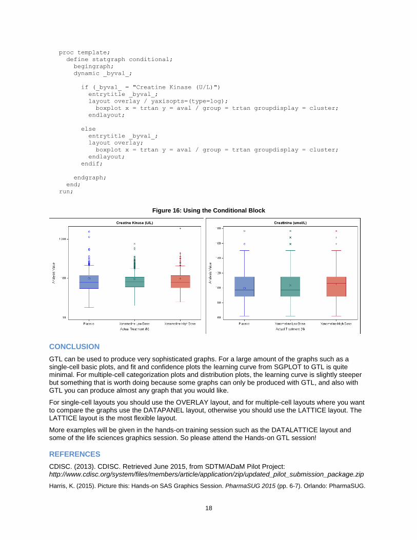
In Figure 15 you can see that there are unusually high Creatine Kinase values, and therefore using the log transformed scale may be a better approach, as seen in Figure 16.

The code below uses the conditional block to output the Creatine Kinase values on the log scale. The dynamic variable _byval_ has been defined below and works in conjunction with the variable in the by statement. The _byval_ dynamic variable is used for two purposes in the code below. The first purpose is to help evaluate which section of the template should be run, that is if the value is equal to “Creatine Kinase

(U/L)” than the first section of the template with the y-axis on the log scale will be run, otherwise the other section will be run with the y-axis on the default linear scale. The second purpose of the _byval_ statement is to assign a title to the figures. The statement entrytitle _byval_, does this. Figure 16 shows the result of using the conditional block.

18

proc template;

define statgraph conditional;

begingraph;

dynamic _byval_;

if (_byval_ = "Creatine Kinase (U/L)")

entrytitle _byval_;

layout overlay / yaxisopts=(type=log);

boxplot x = trtan y = aval / group = trtan groupdisplay = cluster;

endlayout;

else

entrytitle _byval_;

layout overlay;

boxplot x = trtan y = aval / group = trtan groupdisplay = cluster;

endlayout;

endif;

endgraph;

end;

run;

Figure 16: Using the Conditional Block

CONCLUSION

GTL can be used to produce very sophisticated graphs. For a large amount of the graphs such as a single-cell basic plots, and fit and confidence plots the learning curve from SGPLOT to GTL is quite minimal. For multiple-cell categorization plots and distribution plots, the learning curve is slightly steeper but something that is worth doing because some graphs can only be produced with GTL, and also with GTL you can produce almost any graph that you would like.

For single-cell layouts you should use the OVERLAY layout, and for multiple-cell layouts where you want to compare the graphs use the DATAPANEL layout, otherwise you should use the LATTICE layout. The LATTICE layout is the most flexible layout.

More examples will be given in the hands-on training session such as the DATALATTICE layout and some of the life sciences graphics session. So please attend the Hands-on GTL session!

REFERENCES

CDISC. (2013). CDISC. Retrieved June 2015, from SDTM/ADaM Pilot Project: http://www.cdisc.org/system/files/members/article/application/zip/updated_pilot_submission_package.zip

Harris, K. (2015). Picture this: Hands-on SAS Graphics Session. PharmaSUG 2015 (pp. 6-7). Orlando: PharmaSUG.

19

Hebber, P., & Matange, S. (2013). Free Expressions and Other GTL Tips. SAS Global Forum 2013 (p. 3). San Francisco: SAS Global Forum.

Matange, S. (2013). Getting Started with the Graph Template Language in SAS: Examples, Tips, and Techniques for Creating Custom Graphs. Cary, NC: SAS Institute Inc.

Matange, S. (2014). Annotate your SGPLOT Graphs. PharmaSUG China 2014. Beijing: PharmaSUG.

McConville, K., & Much, K. (2015). Creating Sophisticated Graphics using Graph Template Language. PharmaSUG 2015 (p. 1). Orlando: PharmaSUG

ACKNOWLEDGMENTS

I would like to thank Adrienne Bonwick for reviewing this paper. I would also like to thank Sharon Carroll for the support she gave me whilst preparing the paper.

RECOMMENDED READING

Matange, S. (2013). Getting Started with the Graph Template Language in SAS: Examples, Tips, and Techniques for Creating Custom Graphs. Cary, NC: SAS Institute Inc.

CONTACT INFORMATION

Your comments and questions are valued and encouraged. Contact the author at:

Kriss Harris SAS Specialists Limited italjet125@yahoo.com http://www.krissharris.co.uk

SAS and all other SAS Institute Inc. product or service names are registered trademarks or trademarks of SAS Institute Inc. in the USA and other countries. ® indicates USA registration.

Other brand and product names are trademarks of their respective companies.