handover in digital cellular mobile communication...
TRANSCRIPT
Handover in Digital Cellular Mobile Communication
Systems
Mahmood Mohseni Zonoozi
B.Sc. (Eng) (Hon), M. E. E.
A thesis submitted inJiLlfilmen.t of the requirements for the degree of Doctor of Philosophy
VICTORIA I UNIVERSITY
z o r-o o -<
Department of Electrical and Electronic Engineering Faculty of Engineering
Victoria University of Technology, Melbourne, Australia
March 1997
^

FTS THESIS 621.38456 ZON 30001005085313 Zonoozi, Mahmood Mohsem Handover in digital cellular mobile communication systems

Abstract
A mathematical formulation is developed for systematic tracking of the random
movement of a mobile station in a cellular envkonment. It incorporates mobility
parameters under generalized conditions, so that the model could be tailored to be
applicable in most cellular environments. This model is then used to characte.lce
different mobility-related traffic parameters in a cellular system. These include the
cell residence time of both new and handover calls, channel holding time and the
average number of handovers per call. It is shown that the cell residence time can be
described by the generalized gamma distribution, while the channel holding time can
be best approximated by the negative exponential distribution. Based on these
findings a teletraffic model that takes the user mobility into account is presented and
is substantiated using a computer simulation. Further, the influence of cell size on
new and handover call blocking probabilities is examined. The effect of the handover
channel reservation on call dropout probability is also examined to determine the
optimum number of reserved channels required for handover. Improvement to
handover performance is investigated in terms of reduction in the number of
unnecessary handovers as well as reduction in handover delay time. For this purpose
an analytical method is developed which determines the optimum hysteresis level
and the signal averaging time under shadow fading. The results are applicable in both
micro- and macro-cellular systems.

Declaration
I declare that, to the best of my knowledge, the research described herein is the result
of my own work, except where otherwise stated in the text. It is submitted in
fulfilment of the candidature for the degree of Doctor of Philosophy of Victoria
University of Technology, Australia. No part of it has already been submitted for any
degree nor is being submitted concurrently for any other degree.
Mahmood Mohseni Zonoozi
March 1997.

Acknowledgment
1 am most grateful to my supervisor, Dr. Prem Dassanayake who has guided me
through this work. I am indebted to him for his unceasing encouragement, support and
advice. I wish to thank my co-supervisor Assoc. Prof. Mike Faulkner, the ex-Head of
Department Assoc. Prof. Wally Evans, the Deputy Dean of Faculty Assoc. Prof.
Patrick Leung, and the Head of Department Prof. Akhtar Kalam.
Many thanks should also go to my fellow research students in the department of
Electrical and Electronic Engineering with whom I had many helpful discussions
throughout the last four years. The memories I shared with Reza, Nasser, Mehrdad,
Omar, Iqbal, Osama, Adrian, Mahabir, Rushan, Zahidul, VaUipuram, Ranjan,
Olivia, Tuan and Mark will always be in my mind. A special note of appreciation is
extended to the people of Iran who have financed my education for nearly 24 years.
Their sacrifice cannot be paid, I will honour it.
Words cannot express my deepest gratitude and appreciation to my wife, Mahln for her
patience throughout the period of this work when I had to spend all day at my work. She
never ran out of encouragement during the most difficult and vulnerable parts of my stay
in Melbourne. Her emotional support and motivation helped the speedy completion of
this thesis without which this work may not have materialised. I would also like to
acknowledge my son Farhad who throughout many late nights stayed with me at the
university putting independent efforts in learning so many details about computing and
computer technology that projected his ability and tenacity with a mature image and won
him the admiration of many staff and students in the department. My acknowledgement
extends to my littie beautiful daughter Shahrzad for assuring me with her pleasant smile
and sweet warmth while she was around whenever work turned tense. Last but by no
means least, my mother, mother-in-law, father and father-in-law should be
recognized for their everlasting encouragement and support.

With love to my wife Mahin
Table of Contents
Abstract i Declaration ii Acknowledgment iii Table of Contents v List of Fi.gures viii List of T.-bles x Acronyms xi Notations xiii
Chapter 1. Introduction 1
1.1. Historical Overview 2 1.2. Ongoing Work and the Future 6 1.3. Scope of Thesis 11
1.3.1. Effect of mobility on handover 11 1.3.2. Effect of handover on teletraffic performance criteria 11 1.3.3. Effect of propagation environment on handover decision making 12
Chapter 2. Trends in Handover Processes 13
2.1. Cell Stmctures 15 2.2. Handover Performance Measures 17
2.2.1. Performance evaluation by means of traffic analysis 18 2.2.2. Performance evaluation by means of handover administration 18
2.3. Handover Algorithms 19 2.3.1. Signal strength based handover algorithm 20 2.3.2. Co-channel interference based handover algorithm 21 2.3.3. BER and pseudo BER based handover algorithm 21 2.3.4. Distance based handover algorithm 23 2.3.5. Velocity adaptive handover algorithm 23 2.3.6. Direction biased handover algorithm 25 2.3.7. Multi-criteria based handover algorithm 26
2.4. Handover Strategies 27 2.4.1. Network Controlled Handover (NCHO) 27 2.4.2. Mobile Assisted Handover (MAHO) 29 2.4.3. Mobile Controlled Handover (MCHO) 30
2.5. Soft handover 31 2.6. Conclusions and Summary 35
Table of Contents vi
Chapter 3. Stochastic Mobility Modelling 36
3.1. Tracing of amobile inside the cell 38 3.2. Tracing of mobile outside the cell 48 3.3. Conclusions 52
Chapter 4. Cell Residence Time and Channel Holding Time Distributions 53
4.1. Cell Residence Time Distribution 57 4.1.1. Simplified Case , 58 4.1.2. Generalized Case 62
4.2. Mean Cell Residence Time 76 4.3. Effect of Change in Direction and Speed 78 4.4. Average Number of Handovers 85
4.4.1. Method 1 86 4.4.2. Method II 88
4.5. Channel Holding Time Distribution 91 4.6. Conclusions 97
Chapter 5. Effect of Handover on the Teletraffic Performance Criteria.... 98
5.1. Radio Resource Allocation 99 5.1.1. Fixed Channel Assignment (EGA) 100 5.1.2. Dynamic Channel Assignment (DCA) 100 5.1.3. Flexible Channel Assignment 102
5.2. Teletraffic Performance Parameters 104 5.2.1. Setup channel blocking probability 104 5.2.2. New call blocking probability 105 5.2.3. Fixed network blocking probability 105 5.2.4. Handover attempt failure probability 106 5.2.5. Dropout probability 106 5.2.6. Unsuccessful call probability 108
5.3. Teletraffic Analysis 108 5.4. Handover Prioritization Schemes 113
5.4.1. Reserved channel scheme 114 5.4.2. Queueing prioritization schemes 118
5.5. Simulation model 121 5.5.1. Cellular Mobile Coverage Area 122 5.5.2. Analysis of computer simulation results 123
5.6. Conclusions 132
Chapter 6. Mobile Radio Channel Modelling for Handover Analysis 134
Table of Contents vii
6.1. Radio Signal Components 135 6.1.1. Multipath fading component 136 6.1.2. Shadow fading component 138 6.1.3. Path loss component 139
6.2. Mobile Radio Channel Characterization for Handover Analysis 143 6.3. Conclusions 148
Chapter 7. Optimum Hysteresis Level, Signal Averaging Time and Handover Delay 149
7.1. Handover Initiation Parameters 152 7.2. Received Signal Statistics 155
7.2.1. Mean of the received signal level 156 7.2.2. Variance of the received signal level 156
7.3. Handover Algorithm with Hysteresis 159 7.4. Unnecessary Handovers 162 7.5. Handover Delay 170
7.5.1. Handover delay in macrocells 171 7.5.2. Handover delay in microcells 176
7.6. Conclusions 178
Chapter 8. Conclusions 180
8.1. Effect of mobility on handover 181
8.2. Effect of handover on teletraffic performance criteria 182 8.3. Effect of propagation environment on handover decision making 183
References 185
Appendix A User Distribution 203 Appendix B User's Speed Distribution 206 Appendix C Minimum Value of Two Random Variables 208 Appendix D Expected Value of a Distribution 210 Appendix E Source Codes 212
List of Figures
Fig Fig Fig Fig Fig
Fig Fig Fig Fig
1.1 2.1 3.1 3.2 3.3
3.4 3.5 3.6 3.7
Fig.3.8
Fig-Fig.
3.9 3.10
Network development and integration 10 A typical components of a cellular system 14 Trajectory of a randomly moving mobile in the cellular environment 38 Four different cases for a mobile path 39 An example for movement of a mobile from location A to E passing through the regions of 1 (ABC), 2 (CD), & 4 (DE) 42 Illustration of different regions 42 Movement of mobiles between different regions 44 Permissible state diagram for mobile movement 46 Relations to trace a mobile between different regions 47 Coordinates of a mobile position at point A with respect to two different coordinates systems 49 Neighbour cells numbering 49 Geometric relations between real location of a mobile A, and its image A' in the substitute cell 51
Fig.4.1 Representation of cell residence time in time and space domains for a mobile moving across cells 57 Cell residence time illustration for two different cases 60 Simplified flow diagram for analysing boundary crossing 64 Mobile movement in permissible directions 67 New and handover calls' cell residence time distributions obtained analytically (Eqs. (4.6) and (4.9)) and by simulation with the same assumptions 70 Paths of five sample mobile users 71 Examples of generalized gamma density functions 73 New call cell residence time pdf 76 New and handover call cell residence time cdf obtained by the simulation and by the assumption of the equivalent generalized gamma distributions 77 Effect of change in mobile direction on the boundary crossing probability.80 Excess cell radius for different values of drift limits (in degrees) 83 Excess cell radius for different values of mean initial speed 84 Cell residence times for a mobile travelling across cells 89 Average number of handovers experienced by a call for different probabilities of handover failures 91 Illustration of handover within various call duration 92 Illustration of the new and handover call cell residence time 93 Cdf of different random variables for a cell size of 3 Km 95 Variation of the average channel holding time with cell size in the reference cell 96
Fig.5.1 Markov chain representation of two cells with n channels 109
Fig.4.2 Fig.4.3 Fig.4.4 Fig.4.5
Fig.4.6 Fig.4.7 Fig.4.8 Fig.4.9
Fig.4.10 Fig.4.11 Fig.4.12 Fig.4.13 Fig.4.14
Fig.4.15 Fig.4.16 Fig.4.17 Fig.4.18
List of Figures jx
Fig.5.2 Blocking probabilities for the networks with reserved channel scheme .... 116 Fig.5.3 Efficiency of the reserved channel scheme 117 Fig.5.4 Layout for a toroidal 49-cell system (reuse cluster for the cell number 33
highlighted) 123 Fig.5.5 New and handover call blocking probabilities for different cell sizes 124 Fig.5.6 Comparison of offered traffic for different cell sizes 125 Fig.5.7 Dropout probability versus handover call blocking probability. (No channel
reservation) 126 Fig.5.8 Dropout probability versus new call attempt rate. (No channel reservation)...
127 Fig.5.9 New and handover call blocking probabilities with reserved channels for
handover calls 128 Fig.5.10 Dropout probability variation with the number of reserved channels for
handover 130 Fig.5.11 Optimum number of reserved channels for different dropout levels 131 Fig.6.1 Illustration of the parameters for determination of the LOS and NLOS path
losses 143 Fig.6.2 Digital filter for producing slow fading signal component 146 Fig.6.3 Received signal level along a LOS and a NLOS streets in a microcell with
superimposed correlated shadow fading 147 Fig.6.4 Received signal level along a path in a macrocell with superimposed
correlated shadow fading 147 Fig.7.1 Control channel measuring sequence. Cell number 0 stands for the current cell
and other cell numbers stand for the neighbour cells [61] 155 Fig.7.2 Standard deviation as a function of averaging period 160 Fig.7.3 Received signal level from two base stations without shadow fading 161 Fig.7.4 Conversion of the normal distributions to the equivalent standardized normal
distributions 164 Fig.7.5 Unnecessary handover probability versus path loss difference normalised to
hysteresis level 166 Fig.7.6 Effect of shadow fading variance and hysteresis level on unnecessary
handover probability 167 Fig.7.8 Relation between three parameters of h, T, Pu 168 Fig.7.7 Unnecessary handover probability versus hysteresis level for different signal
averaging time 169 Fig.7.9 Definition of parameters for delay calculation 171 Fig.7.10 Handover delay versus hysteresis levels for different signal averaging periods
and cell sizes 174 Fig.7.11 Handover delay versus signal averaging period and hysteresis level as a
function of unnecessary handovers for different cell sizes 175 Fig.7.12 Illustration of handover delay parameters in a micro-cell (figure (b) shows a
zoomed region of figure (a) around the optimal point) 177 Fig. A. 1 User distribution in a strip 204 Fig.C. 1 Region for a random variable Z which is the minimum of the two other
random variables 210
List of Tables
Table 3.1 Equations for calculation of mobile new location 46 Table 4.1 Different distributions derived from generalized gamma distribution 73 Table 4.2 Best fitted gamma distribution parameters value for the new and handover
call residence time 74 Table 4.3 Comparison of results obtained from (4.25)-(4.26) with (4.23)-(4.24) 79
Acronyms
ADC ALT AMPS AR-1 BCC BER B-ISDN CBD Cdf CDMA CDPC CEC CEPT CT DCA DECT EIA ETSI FIFO FCA FDMA FPLMTS GoS GSM IID IN INMARSAT IP IS ISDN ITU IVHS JDC IMPS LCR LEO MAHO
American Digital Cellular Automatic Link Transfer Advanced Mobile Phone Service Auto-Regressive of the first order Blocked-Calls-Cleared Bit Error Rate Broad-band Integrated Services Digital Network Central business district Cumulative distribution function Code Division Multiple Access Cellular Digital Packet data Commission of the European Conununity Conference Europeenne des postes et Telecommunications Cordless Telephone Dynamic Channel Assignment Digital European Cordless Telecommunications Electronic Industries Association (US) European Telecommunications Standards Institute First-In-First-Out Fixed Channel Assignment Frequency Division Multiple Access Future Public Land Mobile Telecommunication Systems Grade-of-Service Global System for Mobile communications^ Independent and Identically Distributed Intelligent Networks International Maritime Satellite Organization Internet Protocol Interim Standard (TIA/EIA cellular network signalling standard, US) Integrated Services Digital Network International Telecommunication Union Intelligent Vehicle Highway Systems Japanese Digital Cellular Japanese Mobile Phone System level crossing rates Low Earth Orbit Mobile Assisted Handover
This abbreviation earlier stood for Groupe Speciale Mobile
Acronyms xu
MBPS Measurement-Based Priority Scheme MCHO Mobile Controlled Handover MSS Mobile Satellite Systems MSC Mobile Switching Centre NCHO Network Controlled Handover NMT Nordic Mobile Telephone PACS Personal Access Communications Services PCS Personal Communication System Pdf Probability density function PHS Personal Handyphone System PIN Personal Identification Number PMR Private Mobile Radio PN Pseudo random Noise PSTN Public Switched Telephone Network QoS Quality-of-Service QPSK Quadrature Phase Shift Keyed RACE Research on Advanced Communications for Europe RSS Received Signal Strength RV Random variable SAT Supervisory Audio Tone SER Symbol Error Rate SIR Signal to Interference Ratio SRS Sub-Rating Scheme TAGS Total Access Communications System TDMA Time Division Multiple Access TIA Telecommunications Industry Association UDPC Universal Digital Portable Communications UMTS Universal Mobile Telecommunication System UPT Universal Personal Telecommunication WAGS Wireless Access Communications Systems ZCR Zero Crossing Rates
Notations
Generic notations and operators
Cov{x) Auto-covar iance function E{ ] Expecta t ion operator F^{x) Cdf of the r andom var iab 'e x . 1Q{ ) Modified Bessel function of the first k ind zero order. Prob{ } Probabil i ty operator /? (T) Auto-correlat ion function of random variable x U{ ) Uni t step function Var{X} Variance of the r andom variable x {X, Y), {X', Y') Coordinate systems with the origin locating at the base station site x\ Y R a n d o m variable x given random variable Y X Mean of random variable x . f^{x), f{.x) Pdf of the r andom variable x r{a) G a m m a function
Degrees 3"'[ ] Inverse Fourier t ransform
Variables
A^^,,i Cell area BC„ . Status of fc"i mobi le in a cell with the of radius nR c N u m b e r of channels allocated to a cell C/, N u m b e r of reserved channels CoriAd) Spatial correlat ion between two signal samples separated by a dis tance Ad D Dis tance between two Base stations D^ M i n i m u m distance to prevent co-channel interference H N u m b e r of handovers per call K Normal izat ion constant K^^, Normal ized cell size with respect to the speed K^, K^ Proport ionali ty factor L Drop in signal level at the street comer in dB. L^, Median path loss in decibels L{x) Path loss for L O S Liy) Path loss for N L O S M Mobi le populat ion in a cell
Notations xiv
N Number of cells p^ Overall blocking probability per cell p„; Fixed network blocking probability Pg _ New call blocking probability Pg Setup channel blocking probability p^ Dropout probability Pj-i^ Handover attempt failure probability p^j Probability of a handover call being delayed Py Unnecessary handover probability p^^ Unsuccessful call probability PiB\a= 0) Boundary crossing probability in the reference cell P(B\a= (p) Boundary crossing probability in a cell with a drift in the range (-cp, + 9) P(0) Normalizing factor P(i) Probability of be ing in state i p^^ Probability that a non-failed handover call requires another handover p^^ Probability that a non-blocked new call requires at least one handover p^^ Transmitter signal power in dB p . Received signal power in dB R Radius of the equivalent circle for a hexagonal cell p#« Region No. n Ri^^,^ Cell radius for a hexagonal cell shape p ' " Radius of a cell in which mobiles move with zero drift (similar to the
reference cell) and a trancated Gaussian speed pdf with an average value of v?i L and standard deviation of a^ = {v-5)/'i[Km/h]
R^ Radius of a cell in which mobiles move with a drift pdf in the range (-(p°, + 9°) and speed pdf similar to that of the reference cell.
s Normal variable denoting local mean signal level in dB. s^if) Power spec tmm of the shadow fading S{n) n" sample of the slow fading signal level SER- Symbol error rate for the base station i T Received signal averaging time T,^ Channel holding time of the handover call. 7/y Channel holding time of the new call 7, Call holding time T.,, Channel holding time in a cell 7/, Handover call cell residence time T New call cell residence t ime V(,, vg Mobile initial speed V, v^., v_ , v Mobile current speed v , , V ^ Mobile previous speed v,„ Maximum mobile speed Km/ii v,„,, Max imum mobile initial speed Km/ti v^^^.^^ Min imum mobile initial speed Km/h u'"h!c Location, scale and shape parameters of the generalized gamma
Notations XV
'#0
distribution d Dis tance traversed by the mobi le ./,„ M a x i m u m shadow fading rate //.(/; a,b,c) General ized g a m m a pdf fl{[i^.) Laplace transform of the handover call cell residence time y ,](ti,.) Laplace transform of the new call cell residence time h Hysteresis level /!/, Base station effective antenna height n M a x i m u m number of calls in a cell «, N u m b e r of calls in cell 1 ^2 N u m b e r of calls in cell 2 p{n^, n^) Steady state probabil i ty of having n, calls in cell 1 and n^ calls in cell 2 Po Normal izat ion constant p„ Received signal strength power at a distance of x P, Transmit ter output power q F o r m factor r R a n d o m received signal level r Sample mean of the received signal level
Estimated received signal level from the communicating base station, BSO Estimated received signal level from the neighbouring base station BS\
r{t) Received signal level in t ime domain r(x) Received signal level in the space domain r,,{t) Mult ipath fading component t\,{,x) Mult ipath fading component in the space domain r„ R a n d o m mult ipath fading component r, Sampled signal level at t ime IAT s,,it) Local mean signal level (shadow fading component) i„(x) Local mean signal level (shadow fading component) in the space domain j„ R a n d o m shadow fading component .V Normal variable denoting local mean signal level in db IQ M a x i m u m channel holding t ime (A, V) Locat ion of a mobi le in a cell with respect to its own coordinate sys tem (A', V') Corresponding location of a mobile in the replaced cell coordinate sys tem (A'|,.y'|) Locat ion of a mobi le in a cell with respect to the neighbour cell
coordinate system A„ Fictitious transmitter point from the base station x^ Breakpoint distance AL Difference be tween the two received signal levels AP„ Excess cell radius for a cell with the radius of P„ AP,, Excess cell radius for a cell with the radius of R^ Ad Dis tance between two signal samples AT" Period between sampl ing t imes AT Time interval between two successive locations of a mobile (P , 0 ) Location of a collection of mobiles in different cells in polar coordinates
Notations xvi
at instant of t . a Magnitude of the change in direction of the mobile with respect to the
current direction in the range (-9°, + <p°) a„ Initial direction angle of the mobile, also the start angle of the mobile 's
new direction in the substitute cell. a Amount of change in direction at instant of t with respect to the
previous direction. p Magnitude of the angle between line joining the mobile's current position
to the reference point (base station), and its previous direction at the instant of T .
7 Propagation slope factor Y Supplementary angle between the mobile's current direction and the line
connecting the mobile's previous position to the base station. 5 Maximum divergence between two observed and hypothesized
distributions. 5„ Hysteresis delay in macrocells 5/ ^ Handover delay in macrocells 5,, Hysteresis delay in microcell 5, Handover delay in microcells 5P„(B) Relative boundary crossing probability between drift of 0° and drift in
the range (-9°, + 9°) e, Reserved channel efficiency ^ Fraction of the average non-blocked new calls out of average total number
of calls in a cell ri Angle between two successive locations of a mobile e, Location angle of the mobile with respect to the original cell e. Location angle of the mobile with respect to the substitute cell 0 Location of the mobile at time T in polar coordinates (angle) X Wavelength x,^ Handover call arrival rate per cell A,„ New call arrival rate per cell Xi Total call arrival rate per cell M Logarithmic average of the received signal local mean power [dBm]. M„,Mi Average received signal levels from the communicating and the
neighbouring base stations Ho(./), Ho(J) Average received signal levels from the communicating and the
neighbouring base stations at a point d from BSO n . Call completion rate. |i /, Total channel service rate [i^. Effective call completion rate [i,^ Handover rate ia,, Average initial speed of mobi le [Km/h] in reference cell \i\, Average initial speed of mobile [Km/h] ^ ' Offset value from the Rayleigh distribution (amplitude of direct wave)
Notations xvii
n Number 3.14 p Autocorrelation factor pj Spatial correlation factor at a distance d^ p . Total effective traffic intensity per cell p,^ Offered traffic per cell by handover calls p^ Offered traffic intensity p Location of the mobile at time x in polar coordinates (magnitude) p(,, 00 Initial location of a mobile in polar coordinates iPnk' ^nk^ Location of A:* mobile in a cell of radius nR at time x in polar coordinates (p:fr0 ) Location of a mobile at time x in polar coordinates o Standard deviation of the received signal in dB a^ Standard deviation of the shadow fading in dB 0^ Standard deviation of the initial speed of mobile [Km/h] X Time after initiation of a call (p Range of change in direction of mobile. (p(0 Phase angle of the received signal ^{Q,\) Normal variable with mean of o and standard deviation of i 9t Equivalent reference cell radius for a cell supporting freedom on mobile's
drift with a uniform pdf in the range (-9°, + 9°) and speed pdf similar to that of the reference cell.
•31^^ Equivalent reference cell radius for a cell supporting freedom on mobile's drift with a uniform pdf in the range (-9°, + 9°) and speed with a tmncated Gaussian speed pdf having an average and standard deviation different from reference cell.
9?^ Equivalent reference cell radius for a cell supporting freedom on mobile's speed with a tmncated Gaussian pdf having an average and standard deviation different from reference cell. Mobiles are allowed only to move on straight path without any drift.
Chapter 1
Introduction
The worldwide communication network is probably the greatest achievement of the
mankind. Many aspects of our lives today are dependent on this network so that even
a modest failure of it would impact on our lives by way of a major dismption of our
day to day activity in this modem society. The conventional telephone network,
better known as the Public Switched Telephone Network (PSTN), that provides
national and intemational coverage through its fixed stmcture has been in existence
for a considerable time. However, the emerging trends indicate that the evolution of
communication from place based system to a person based system has already begun
and its universal spread is imminent. Having access to information and being able to
communicate easily and securely, in any medium or a combination of media (voice,
data, image, video, or multimedia) in a cost effective manner is something that has
taken for granted by the modem society. Further, the importance of such systems is
Chapter 1: Introduction
highlighted by the fact that the mobile communication faciUty advocates the notion
that communication should be possible at any time from any where to any one. It is
believed that in next decade the portable phone will replace the 'telephone in the
house' of today. The cellular mobile radio systems have been recognised as the most
promising stepping stone to this future goal. It is anticipated that the expansion of
cellular communication networks will be a major activity throughout the v;r)rld in
this decade.
1.1 Historical Overview
In the early mobile systems a user was free to move only within the coverage area of
a single base station. In these systems, known as Private Mobile Radio (PMR), each
user was allocated a particular frequency band (channel). However, to really allow
the users to be mobile, the service area has to cover a wide region. This would
involve a large number of users and the required number of channels could not be
found within the available spectmm. Therefore, the cellular concept of using the
same frequency at different places was introduced by MacDonald [1] in 1979. The
cellular concept allows an infinitely large area to be served by a hmited frequency
band. In a cellular system the entire area in which the network operates is divided
into cells, and the available spectmm is shared among a cluster of cells. The clusters
are repeated to cover the entire area. Associated with each cell is a base station which
handles all the calls made by tiie mobiles in the cell area using a set of channels
assigned to the cell.
The first cellular system, AMPS [2, 3], was developed during the 1970s by Bell
Chapter 1: Introduction
Laboratories. This first generation analog cellular system has been available since
1983. It used FDMA technology to achieve radio communications. With FDMA,
voice channels are carried by different radio frequencies. A total of 50 MHz in the
band 824-849 MHz and 869-894 MHz is allocated for AMPS. This spectmm is
divided into 832 frequency channels or 416 downlinks and 416 uplinks. TAGS, NMT
and JMPS are am jfig other first generation cellular system. Although cell division
techniques are frequently employed by the first generation, reduction of cell sizes to
below a few hundred meters would eventually render cell division no longer feasible.
Moreover, analog modulation is sensitive to interference from other users in the
system, and the voice quality is quite vulnerable to various kinds of noise. As a
consequence of these, other means of capacity improvement such as efficient
modulation schemes were sought for the second generation.
In the second generation cellular systems, digital technology enables the use of signal
processing techniques to increase die robustness against interference. It also reduces
the spectral bandwidth required for each user and hence provides higher capacity.
The second generation provides about 3 to 4 times the capacity of the first generation
without adding new base stations. Since digital systems are more immune to noise, a
SIR ratio of 7 dB could be tolerated for a digital system whereas 15 dB is required for
the analog systems under same circumstances [4]. This allows for smaller reuse
clusters, thereby increasing the capacity of the system. The control signalling in the
second generation cellular system can easily be hidden from the users, whereas in the
first generation it appears as annoying noise bursts to the users. Unlike the first
generation where handover decisions are completely managed by the network and
terminals are passive in the handover process, in the second generation the terminals
Chapter 1; Introduction
are active in the handover process by supplying measurement values to the network.
In the second generation, three major cellular systems (namely GSM [5], ADC [6],
JDC [7]) have been launched that employ a circuit switching hybrid FDMA/TDMA
scheme on the radio channel, and there is another standard under evaluation that uses
CDMA technology [8, 9, 10].
GSM is widely used in Europe, Australia and Asia. In GSM every frequency carrier
is divided into fixed time slots that supports up to eight voice channels. The speech
coding rate is 13 Kb/s in GSM. With TDMA, the radio hardware in the base station
can be shared among multiple users. In North America, however, the main design
objective has been to make a smooth transition from the low capacity analog systems
to high capacity digital systems. This is possible since digital technology enables
allocation of three TDMA channels on the same radio frequency as one FDMA
channel in the AMPS system. Such a mixed system, known as ADC (DAMPS or
IS-54 standard) enhances the capacity of the system three times just by exchanging
the analog FDMA transceivers to digital TDMA transceivers. The speech coding rate
is 7.95 kb/s in ADC. The Japanese have designed a digital system, known as JDC
where the transmission part resembles the American IS-54 standard and the protocols
for communication resembles the GSM standard. JDC and ADC systems have high
modulation efficiency due to the use of QPSK modulation and low bit rate codecs.
Therefore both systems have more system capacity than GSM.
Recently a new standard employing CDMA technology, IS-95, has been developed
in North America which claims to have many advantages over TDMA technology,
including improvement to capacity up to 10 to 12 times over the analog systems.
Chapter 1; Introduction
However, these claims have not yet been fully accepted by the advocates of TDMA
and the issue is still of considerable controversy. At the moment the CDMA standard
is undergoing field tests.
Another system, similar to the cellular system, which has the same basic purpose of
providing its users access to the PSTN without any .constiaint of a wire connection, is
the cordless telephone system. In a cordless telephone system each user has his/her
own base station attached to his/her subscriber line. In general, the digital cordless
systems are optimized for low-complexity equipment and high-quality speech in a
quasi-static environment (with respect to user mobility). Conversely, the digital
cellular air interfaces are geared toward maximizing bandwidth efficiency and
frequency reuse. This is achieved at the price of increased complexity in the terminal
and base station. While a cordless phone and its base station comprise an autonomous
communication system, cellular phones rely on complicated coordination under the
control of a central processor. In a similar manner to the cellular systems, the
cordless telephone system has undergone a change from an analog stage (first
generation) to a digital revolutionary phase (second generation). The diird generation
mobile systems will be an integrated service facility which will combine the cellular
and cordless services.
The most serious drawback of the first generation cordless telephone is the operating
range which is limited to tens of meters from a single base station. Another big
problem is the vulnerability to interference from other cordless telephones. Most of
the first generation cordless telephones have access to only one channel and the user
can do nothing to avoid interference from someone nearby using the same channel.
Chapter 1: Introduction
Of the cordless phones that have access to several channels, almost all rely on manual
channel selection to avoid interference. The second generation cordless phone is able
to communicate with many base stations and it automatically selects the best
available radio channel. Examples of this system are CT2 [11], DECT [12], PHS [13,
14], WACS [15, 16] and PACS [17].
1.2 Ongoing Work and the Future
The current demand for mobile communication facilities and the dramatic increase in
its growth rate reveal that even the second generation systems cannot be expected to
fulfil all demands. Moreover, with emerging multimedia applications it is beheved
that an entirely new generation cellular system is required to handle the new
applications. Continuous improvements in microelectronic technology and radio link
techniques coupled with advances in network signalling and control capabilities will
support increasingly sophisticated featiires and services. Part of the challenge in
planning future wireless systems is to determine the services that they would be
required to support. It is not unrealistic to envision in very near future subscribers
with small pocket-size flip-top terminals with keyboard and display being capable of
originating or receiving calls of voice, video and data including fax and electronic
mail. The ability to integrate these services and convert between media will give the
subscriber not only the abihty to select the most convenient terminal, but also the
most convenient medium.
During the development phase of the GSM system another research initiative was
launched by the European Community to develop an advanced communication
Chapter i: Introduction
network for Europe which is intended to incorporate the same service on fixed as
well as on mobile radio networks. The idea is to establish a Personal Communication
System [18, 19] (PCS^) that allows mobility of both users and services. The main
feature of PCS is the concept of personal mobility. Whether a subscriber is in the
house, in the car or in the office, they should be able to use the same terminal, at any
time with any of the allowed access methods using their personal identification
number. In addition, the advanced service features and variety of data transmission
types will have to be supported by such systems. It is anticipated that PCS wiU need
an enormous capacity, which must be met with new technology. The mixture of
applications implies that new access methods must be negotiated in order to host
different data types, such as speech and video. Also the cell sizes have to become
smaller to allow higher capacity in city environments. Since the users of cellular
phones are getting used to pocket sized telephones, one cannot expect that the phones
of PCS to be any larger. Therefore, the batteries have to be efficient enough to allow
the use of high power transmissions in mral areas.
There are some situations in which providing radio coverage with terrestrial based
cellular networks is either not economically viable (such as remote,
sparsely-populated areas), or physically impractical (such as over large bodies of
water). In these cases, satellite based cellular systems can be the best solution [20].
By the use of many LEO satellites a complete coverage of the world is possible with
low power telephones. Motorola's Iridium project [21] is an example of such a
system. It seems that PCS will consist of a mixture of technologies, and the mobile
PCS is termed by International Telecommunication Union (ITU) as Universal Personal Telecommunication (UPT).
Chapter 1: Introduction
terminal must be able to switch between systems so that a system tiiat fits the user's
occasion best is used. In this case, another kind of handover, to be referred as
intersystem handover, will be essential.
It is conceivable that the current pan European digital mobile telephone network will
not satisfy the telecommunication needs of a future society in terms of user capacity
and service provisions. To satisfy the needs of future customers of mobile
telecommunication services the Commission of the European Community (CEC) has
launched an ambitious research initiative under the Research on Advanced
Communications for Europe (RACE) program. The program's purpose is to study
and develop the enabling techniques for creating a third generation mobile
communication system by the turn of the century and to integrate similar services as
provided in fixed networks such as ISDN and B-ISDN. Therefore, it is necessary to
study the technological aspects of mobile telecommunications to see how they can
influence its user capacity and services.
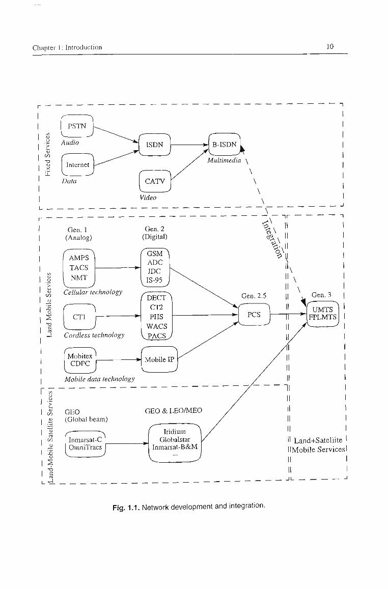
It is anticipated that the third generation wireless systems (e.g. FPLMTS, UMTS [22,
23]) will be operational by the year 2000. These would aim to consolidate on the
developments and services (voice, video, data, etc.) offered by fixed (PSTN, ISDN),
cordless, paging and cellular mobile (terrestrial and satellite) networks, to form a
common integrated network. The transmission plan for this new global system needs
to be flexible enough to support both personal and terminal^ mobilities. The
emergence of the third generation wireless system is set to make a lasting impact on
Terminal mobility is accommodated using a portable terminal through a wireless access to a fixed base station. Personal mobility can be accommodated either through a wired access or through wireless access using a portable identity card [24].
Chapter i: Introduction
the telecommunication field. However achieving its goals will be a long-drawn-out
task with many stumbling blocks to overcome. The most important issue here is
related to the large amount of signalling information which the network has to handle
in paging, channel assignment, handover, user location updating, registration,
security clearance, and the like. Fig. 1.1 illustrates some perspectives of this network
development and its integration trend.
Chapter I; Introduction 10
•a
Vie
<u o -o aj ti;
^ "1 PSTN
L J Audio
C ^ Internet
I J Data
Multimedia \
\
Video
Land+Satellite Mobile Services
Fig. 1.1. Network development and integration.
Chapter 1: Introduction 11
1.3 Scope of Thesis
This thesis is focused mainly on three important issues concerning the handover
process in cellular mobile systems. These include the following:
• Effect of mobility on handover,
• Effect of handover on teletraffic performance criteria,
• Effect of propagation environment on handover decision making.
1.3.1 Effect of mobility on handover
In Chapter 3 a mathematical formulation is developed for systematic tracking of the
random movement of a mobile station in a cellular environment. It incorporates
mobility parameters under most generalized conditions, so that the model could be
tailored to be applicable in most cellular envhonments. Using the developed mobihty
model, the characterisation of different mobility-related parameters in cellular
systems is studied in Chapter 4. These include the distribution of the cell residence
time of both new and handover calls, channel holding time and the average number
of handovers per call. It is shown that the cell residence time can be described by the
generalized gamma distribution while the channel holding time can be best
approximated by negative exponential distribution [25- 36].
1.3.2 Effect of handover on teletraffic performance criteria
Chapter 1: Introduction 12
Based on the results obtained for cell residence time distribution, a teletraffic model
that takes user mobility into account is formulated in Chapter 5. This is supported by
a computer simulation using the next-event time-advance approach also described in
Chapter 5. Furthermore, the influence of cell size on new and handover call blocking
probabilities is examined. The effect of the handover channel reservation on call
dropout probability is investigated to determine the optimum number of reserved
channels required for handover [37- 39].
1.3.3 Effect of propagation environment on handover decision making
A mobile radio channel is usually characterized by superposition of three
independent components which reflect small-, medium-, and large-scale propagation
effects. In Chapter 6, contributions of each of these components are considered.
Emphasis is made on the effect of shadow fading (the medium-scale propagation
component), which is important in handover decision making in cellular networks.
In Chapter 7, improvement to handover performance is investigated in terms of
reductions in unnecessary handovers and handover delay time. An analytical method
is described to determine the optimum hysteresis level and signal averaging time for
both micro- and macro-cells. Resuhs demonstrate the possible compromise between
handover parameters, i.e. signal averaging time and hysteresis level, under the
influence of shadow fading. These resuhs could be used in setting the parameters of
the handover algorithm to minimise delay in handover decision making while
minimising unnecessary handovers [40- 46].
Chapter 2
Trends in Handover Processes
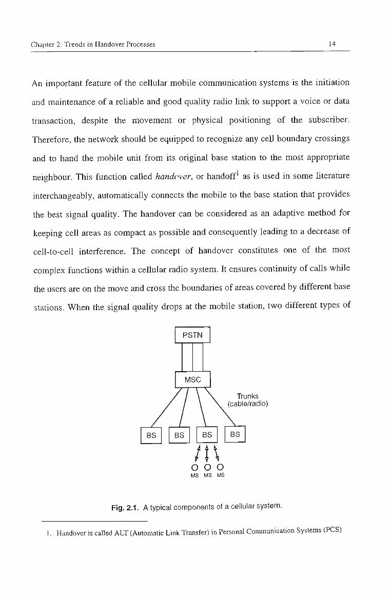
A cellular network can be viewed as an interface between mobile units and a
telecommunication infrastmcture (e.g., PSTN). A mobile station (MS) is a
low-power communication device that has a limited radio coverage area with radius
ranging from a few kilometres (macrocells) to several hundreds of meters
(microcells). In a cellular environment, a large geographical area is divided into
small areas each covered by a cell-site or base station (BS). When an MS places a
call, a dedicated circuit has to be established between the MS and the called party.
The first link of the circuit is a wireless link between the MS and the closest BS. The
second link is estabhshed between the BS and mobile switching centre (MSC), which
can be through a wireless or a wired media. A typical cellular system is illustrated in
Fig. 2.1 [47].
Chapter 2: Trends in Handover Processes 14
An important feature of the cellular mobile communication systems is the initiation
and maintenance of a reliable and good quality radio link to support a voice or data
transaction, despite the movement or physical positioning of the subscriber.
Therefore, the network should be equipped to recognize any cell boundary crossings
and to hand the mobile unit from its original base station to the most appropriate
neighbour. This function called handover, or handoff as is used in some hterature
interchangeably, automatically connects the mobile to the base station tiiat provides
the best signal quality. The handover can be considered as an adaptive method for
keeping cell areas as compact as possible and consequentiy leading to a decrease of
cell-to-cell interference. The concept of handover constitutes one of the most
complex functions within a cellular radio system. It ensures contmuity of calls while
the users are on the move and cross the boundaries of areas covered by different base
stations. When the signal quality drops at the mobile station, two different types of
Trunks (cable/radio)
o o o MS MS MS
Fig. 2.1. A typical components of a cellular system.
1. Handover is called AUT (Automatic Link Transfer) in Personal Communication Systems (PCS)
Chapter 2: Trends in Handover Processes 15
handover, namely inter-cell or intra-cell, could take place. In cases when there is a
strong interferer on a channel, it may be sufficient to switch to another channel, but
remain connected to the same base station. This type of handover is called an
intra-cell handover. The primary purpose of an inter-cell handover is to switch a call
in progress from the serving base station to a neighbouring base station whenever the
existing radio link suffers from degradation.
This Chapter explains briefly issues affecting the handover process, or being effected
by the handover process, explicitly or implicitly. The aim is not to describe each
phenomenon in detail but to present the issues so that the flavour of current trends
could be observed.
2.1 Cell Structures
The dramatic increase in demand for mobile communication systems has motivated
many researchers to place a greater emphasis on maximising the system capacity.
Conventionally the capacity of a network could be enhanced by deployment of
different methods such as efficient modulation schemes, improved speech coding
techniques, appropriate channel coding, frequency spectmm allocation. Nevertheless,
there is an exclusive elaborate approach for increasing capacity in the Cellular
mobile communications systems, and that is by reducing the cell size. Theoretically, 2
a reduction of cell radius by n times could enhance mobile system capacity by n
times. Application of different cell sizes such as: picocells, microcells, macrocells,
mixed cells, overiapped cells, highway microcells appears to be suitable solution to
the complicated problem of different traffic demands in various areas.
Chapter 2: Trends in Handover Processes 16
Implementation of cells of smaller size is seen as the obvious way to increase system
capacity which would effectively cater for higher demands. Smaller cells, however,
come with their own drawbacks in cellular system design. Apart from the network
complexity, the main difficulty is the increased proportion of handovers that occurs
during one particular call.
Labedz [48] has shown that the number of cell boundary crossings per call is
inversely proportional to the cell radius. In addition, Nanda [49] has found that while
the handover rate only increases with the square root of call density in macrocells, it
increases linearly with the call density in microcells. Since the mobile has a certain
probability of encountering a dropped call at every boundary crossing, handover
algorithms must become more robust as the cell size decreases.
Due to the small cell dimensions in microcellular systems, a rapidly moving mobile
will cause a high work load for the handover management system since the mobile
will cross cell borders at a high rate. The rapidly changing signal quality, and
frequent requirement for handovers during a call, leads to the risk of a dropped call in
fast mobiles. It has therefore been suggested that some channels are assigned to base
stations with antennas placed high above the ground level and relatively free from
obstructions. Thus, the coverage areas of these overiaid cells will be large and
therefore the handover rate will be much lower than for microcells, and the call
reliability will improve. For this scheme to be useful, the system must provide some
means to measure the mobile's velocity so that the fast mobiles could be assigned to
umbrella cells. One raw method could be to monitor the frequency of handovers, and
if the terminal has made a large number of handovers within a short period of time, it
Chapter 2: Trends in Handover Processes 17
is probably moving fast and should be connected to an umbrella cell. A moving
terminal also generates a Doppler spread [4] of the received signal, and a large
Doppler spread indicates that the terminal should be handed over from the
microcellular system. The deployment of a multi-tier system with macrocells
overlaying microcells offers system providers new opportunities. Clever use of the
two tiers can lead to increased end-user performance and sy.' iicm capacity. For
example, stationary users can be assigned to microcells so that they operate at
reduced power and cause significantly less interference; when the microcellular
capacity is exhausted, the overflow traffic can be assigned to the macrocells. As
another example, a business area with building and parking facilities may employ
microcell base stations to cover the outdoor areas together with picocells to provide
radio coverage to indoor areas and offices. Behaviour of the handover in all these
circumstances raises issues that need to be discussed.
2.2 Handover Performance IVleasures
Many criteria for determining the efficiency of a handover algorithm are discussed in
the literature [50, 51, 52, 53] and may be used in optimal design. To completely
evaluate the performance of a handover scheme one should build a full system and
collect data for evaluation. This, of course, is not practicable. The second best
method would be to build a complete simulation model of the system and emulate the
actions of users and handover algorithms. This would lead to extremely complex
simulation models which again would not be practicable. Simpler scenarios must
therefore be used focusing attention on particular problems. Solving these individual
problems, one could obtain information necessary to assess the system performance
Chapter 2: Trends in Handover Processes 18
for handover schemes. In this section, different aspects of handover performance
evaluation will be described.
2.2.1 Performance evaluation by means of traffic analysis
To evaluate the effect of handover on the capacity of a cellular system, it is possible
to use traffic performance evaluations. By assuming that originating calls and
handovers to a cell can be modelled as Markovian "birth-death" processes, and that
the unencumbered call duration and channel holding time can be modelled as
negative exponentially distributed random variables, it is possible to obtain analytical
results for a number of performance measures. The unencumbered call duration and
channel holding time are the time for an unintermpted call to be completed, and the
time a user is active on a channel in a cell before the channel is released (by call
completion or handover), respectively. In Chapter 5, different teletraffic performance
parameters are defined. These parameters can be obtained for a number of resource
assignment schemes and platform types.
2.2.2 Performance evaluation by means of handover administration
The methods treated by traffic performance ignores the dynamic performance.
Hence, other methods are needed to evaluate the administration load imposed by the
resource allocation schemes. It is therefore common to identify some scenario that
provides desired information. To establish the tiade-off between the signal quaUty
and the handover management load a commonly used method is to let a terminal
move between two base stations while the signal quality and the handover activity is
Chapter 2: Trends in Handover Processes 19
monitored. This method has been used for simulations in [54, 55, 56] and for analytic
evaluations in [57]. Among the quantities that are monitored durmg one trip are: the
mean number of handovers, probability of unnecessary handovers, duration of
intermption, number of unnecessary handovers, delay in making a handover and the
distance at which handover occurs.
2.3 Handover Algorithms
Handover algorithms are decision systems in which decisions are tiiggered by
channel degradation or network criteria. Channel degradation criterion can be
realized by different measurements such as the received signal strength [54, 58, 59,
60, 61, 62], received signal to interference ratio (SIR) [63], bit error rate (BER) [64,
65], and estimated distance from base stations [60, 66]. In the network criterion, the
handover decisions are made by reasons other than degradation of die current
channel such as teletraffic load and the decisions are taken by die network
management centre of the cellular system. In [67], the handover problem in a
stochastic control frame is introduced and a Markov decision process formulation is
used to derive optimal hanover.
Handover algorithms should be robust to variations in propagation, mobile station
velocity, and co-channel interference. Ideally they should perform only one handover
per cell boundary crossing, and this handover should occur quickly and as close to
the boundary as possible. A literature review of the existing and proposed algorithms
is suinmarized in the following sub-section.
Chapter 2: Trends in Handover Processes 20
2.3.1 Signal strength based handover algorithm
The signal strength based handover algorithm compares signal strength averages
measured over a time interval, and executes a handover if the average signal strength
of an alternative base station is larger than that of the serving base station. This
method is shown to stimulate too many unnecessary handovers when the current base
station signal is still adequate [57, 59, 61, 62]. This problem can be alleviated by
introducing a hysteresis margin. This allows a user to hand over only if the new base
station is sufficiently stronger (by a hysteresis margin) than the current one. This
technique prevents the so-caUed ping-pong effect. The ping-pong effect is the
repeated handovers between two base stations caused by rapid fluctuations in the
received signal strengths from both base stations. This matter is addressed in Chapter
7.
Loew [68] describes a relative signal strength based handover algoritiim which uses
the signal strength difference coupled with an absolute level requirement. In tiiis
manner, the signal strength difference is only compared if the average signal strength
is below an absolute threshold level. Zhang et al. [69] provide an analytical method
to evaluate the performance of this algorithm. Mufioz-Rodriguez et al. [70] provide a
neural circuit to perform this algorithm.
In general, the handover initiation criteria analysed in the literature are based on
essentially four variables: the lengtii and shape of the averaging window, the
threshold level, and the hysteresis margin.
Chapter 2: Trends in Handover Processes 21
Prediction techniques base the handover decision on the expected future value of the
received signal strength. A technique based on this has been proposed and shown
(through simulation) to be better, in terms of reduction in the number of unnecessary
handovers, than both the relative signal strength and relative signal strengtii witii
hysteresis and threshold methods [71].
2.3.2 Co-channel interference based handover algorithm
Although signal strength based algorithms are useful, diey do not take into account of
the co-channel interference. In [63] a handover algoritiim is developed under die
assumption that the mobile station or the base station has access to real time SIR
measurements. Nevertheless, obtaining these measurements is difficult in practice
[72, 73], and only few papers [73, 74, 75] have investigated methods to actually
monitor tiie co-channel interference. Kozono [74] suggests a metiiod for measuring
co-channel interference in the first generation cellular systems, AMPS, by separating
two terms at different frequencies which are both known functions of the signal and
interference. An interference measurement ckcuit is used to perform this separation
and estimate the co-channel interference. Yoshida [73] suggests a metiiod for
in-service monitoring of multipath delay spread and co-channel interference for a
QPSK signal. He reports that the co-channel interference can be monitored for
multipath fading channels provided the delay spread is negligible.
2.3.3 BER and pseudo BER based handover algorithm
Bit error rate based metiiods are desirable since they give a good indicator of speech
Chapter 2: Trends in Handover Processes 22
quality. Steele [65] investigated estimating the BER by counting the number of errors
from the error locator polynomial assuming Reed Solomon encoding. Using tiie
derived symbol error rate SER- for the base station /, the suggested handover
algorithm computes whether SERQ/SER^ is less than some threshold. A variable P •
is assigned a one if it was tme and a zero if it was false, where ; denotes the current
dects lon point. Afterwards, a weighted sum of the P • 's is formed and compared to a
new threshold. A handover is activated if the weighted average is greater than the
threshold, and SERQ is greater than an unacceptable symbol error threshold. Steele
used this algorithm in a two cell cluster, and found a slight delay in handover in the
presence of co-channel interferers. Comett et al. [64] have showed two methods to
estimate the BER in a Rayleigh fading channel. The first derives the BER from an
autocorrelation parameter in the receiver, given that a pseudo random noise sequence
is interleaved in the data. The second shows if symbol interleaving is used in a
Reed-Solomon-based system, then side information from a bounded distance decoder
can be used for a raw channel BER.
Pseudo error rate methods have also been studied in [76, 77]. Kostic et al. [76] have
derived a pseudo error rate method for PSK modulation. Nagura et al. [77] have
investigated the use of the eye-opening as a measure of the signal quality. Here, a
pseudo error is said to occur when the eye-opening height falls below a certain
threshold. The channel is assumed acceptable until the pseudo error rate is above the
threshold and its slope is positive.
Chapter 2: Trends in Handover Processes 23
2.3.4 Distance based handover algorithm
Knowing the distance between mobile station and base station, it is possible to
control the movement of the mobile in the cell stmcture. This avoids using a channel
outside the planned cell area. A variety of methods have been published that
determine the mobile's position in macrocells such as angle of arrival techniques
from multibeam antennas [78] and antenna arrays [79], time-of-arrival methods [80,
81], and cmde signal strength methods [82]. With tiie current interest in intelligent
vehicle highway systems (IVHS), a substantial amount of research is aimed at
investigating these and other methods for vehicle location and tracking in microcells.
Currently known methods are not accurate enough to base handover on position
information alone [83].
2.3.5 Velocity adaptive handover algorithm
If handover requests from rapidly moving mobile stations are not processed quickly,
excessive dropped calls may occur. Fast temporal based handover algoritiims have
been shown to be able to partially solve this problem [61] by using short temporal
averaging windows to detect large, sudden, drops in signal strength. However, the
shortness of a temporal window is a relative quantity to the mobile station velocity
and, furthermore, a fixed time averaging interval makes the handover performance
sensitive to velocity, with best performance being achieved only at a particular
velocity. To overcome tiiis problem, velocity adaptive handover algorithms have
been proposed to provide good and consistent handover performance for mobile
stations having different velocities. Different velocity estimators have been
Chapter 2: Trends in Handover Processes 24
investigated which were based on following techniques:
• Level Crossing Rates (LCR) with respect to the signal envelope;
• Zero Crossing Rates (ZCR) of tiie in-phase and quadrature components of the signal envelope;
• Covariance approximation method;
• Eigen-based Doppler estimation for differentially coherent CPM.
LCR is defined as the average number of times the signal envelope crosses a
specified level in the positive direction. Likewise, ZCR is defmed as the average
number of zero crossings a signal makes per second. It is well known that the LCR or
ZCR are functions of the mobile velocity [4, 84] and can be used for velocity
prediction. Austin et al. [85] has derived a velocity estimator based on the LCRs of
the received signal which is robust to the Rice factor.
Covariance approximation is a velocity estimator method that rehes on an estimate of
the autocovariance between faded samples of the signal. This method is based on
estimating the maximum Doppler frequency as a means to obtain mobile velocity.
The procedure which estimates the Doppler frequency from the squared deviations of
the signal envelope originally is put forth by Holtzman and Sampath [86]. This model
is later shown robust to Rice factors and white Gaussian noise [87].
For some modulation schemes, it may also be possible to measure the velocity from
the Doppler shift in tiie signal. Common methods for Doppler estimation such as
automatic frequency control loops are often inappropriate due to burst intervals
where the acquisition time consumes a large portion of the data interval. Open loop
Chapter 2: Trends in Handover Processes 25
Doppler estimation has been considered [88] for PSK signals and extended to
differentially coherent CPM by Biglieri [89]. Austin [90] considers a generahzation
of Biglieri's method whereby the Doppler is estimated by using a set of averages each
obtained from a separate differential detection of a CPM waveform. The averages are
shown to have the same form as the autocorrelations of a complex exponential at a
known multiple o^he Doppler frequency in noise, and therefore, eigen-based line
spectral estimation methods can be used to estimate the Doppler frequency.
2.3.6 Direction biased handover algorithm
The majority of previous handover algorithm studies [54, 56, 57, 59, 61, 62, 70, 91,
92] have concentrated on handover decisions between two base stations only. Mende
[60] simulated the case of multiple base stations, but no conclusions were made. In
urban microcells, the mobile is likely to have multiple base stations tiiat are handover
candidates at any instant. For example, consider a Manhattan type street layout
consisting of streets on a rectangular grid. One proposed method to cover such an
area is to place base stations at every other intersection. Thus, as soon as a mobile
moves into an intersection without a base station, four base stations become
candidates for handovers. One metiiod to accomplish a proper handover is
encouraging handovers to base stations that the mobile is moving towards and
discouraging handovers to base stations tiiat the mobile is moving away from. Three
basic approaches to accomplish the direction biasing are proposed. The fhrst two
approaches use direction adjusted hysteresis levels, while the tiikd approach uses a
fuzzy handover algoritiim in which the membership functions will be dkection
biased.
Chapter 2: Trends in Handover Processes 26
The direction biased handover algorithms presented only need tiie subscribers'
moving direction; precise position is not necessary. Thus, simpler estimation
techniques can be used; such as monitoring the direction of the Doppler shift
(positive or negative) [89, 90], monitoring the time variation of tiie signal stiengtii, or
even determining the direction from the location of past handovers. Unfortunately,
Doppler (velocity) estimation techniques which derivcestimates from the covariance
or level crossing rates [85, 86, 87] are not useful because these techniques only yield
the magnitude of the Doppler. A simple dhection estimator is based on monitoring
the time variation of the signal strength. Austin [93] has investigated multi-cell
handover characteristics of classical handover algorithms by using a Manhattan
microcell environment with base stations located at every other intersection.
2.3.7 Multi-criteria based handover algorithm
Conceivably, a handover should be made on a variety of statistics that are related to
the capacity of the system. Current systems such as GSM [66] now tiigger a
handover if any individual handover statistic suggests the need for a handover. New
research is just beginning on how to incorporate multiple criteria such as distance,
BER, co-channel interference, signal strengtii, and so on all into a single handover
algorithm. Mufioz-Rodriguez et al. [94, 95] have suggested various fuzzy set
combinations and neural network methods [70] by which various criteria can be
combined into a handover algorithm. Nevertheless, no insight has been given on how
to optimize or choose the various parameters for multiple criteria handover
algorithms. However, a combined BER and signal stiengtii algoritiim is developed by
Kumar et al. [96].
Chapter 2: Trends in Handover Processes 27
2.4 Handover Strategies
The mobile unit and the base station are connected via radio links which carry data as
well as signalling information. In case a signal deterioration occurs, three different
handover strategies have been proposed for transferring the connection to a new base
station [54]. Depending on the handovi^r decision process being applied as a
centralized, half centralized or decentralized phenomena, three different types of
handover strategies can be defined respectively as:
• Network Controlled Handover (NCHO)
• Mobile Assisted Handover (MAHO)
• Mobile Controlled Handover (MCHO)
Since the number of handovers increases with decreasing cell size, it will be an
almost impossible task to make a handover decision for every mobile by one central
switch (centralized). Moreover, in microcells the connection between MS and BS can
deteriorate very quickly. A typical situation is when tiie mobile turns round a street
corner (street comer effect). Fast handover decisions required in such situations can
be achieved more readily by decentrahzing the handover decision process.
2.4.1 Network Controlled Handover (NCHO)
This method is widely used in first generation cellular systems, where the MSC is
solely in charge of the handover process and the mobile stations are completely
passive. The base stations monitor the quality of the current connection by measuring
Chapter 2: Trends in Handover Processes 28
the received signal strength (RSS) of connected stations. Also the signal to
interference ratio (SIR) is measured by means of a supervisory audio tone (SAT).
This is accomplished by the base station transmitting a tone with a frequency outside
the audio range. This tone is echoed by the terminal, and from the received signal the
base station can estimate the degree of interference by evaluating the quality of the
received SAT. If the received signal deteriorates below some threshold, and/or the
quality of the SAT is degrading, the base station sends a request for handover to the
mobile switching centre (MSC). Meanwhile, the MSC orders all the surrounding
base stations to tune into the channel used by the terminal to measure the received
signal strength from the mobile and to respond with the result. The MSC then decides
to which base station the mobile should be handed over, and assigns a new channel
frequency. The new channel is instmcted as to both the mobile (through the old base
station) and the new base station.
Once the target base station and the mobile station are synchronized the handover is
completed. After tiiat the old channel, and tiie link between tiie MSC and the old base
station are released. The signalling involved here leads to a long reaction time in
handover. Further, there is always the possibility of interpreting data as signals in
error leading to failed handovers. The typical handover time, i.e. the time between
detection of a necessary handover and the completion of tiie handover, has been
found to be of the order of 5-10 seconds. Therefore, this type of network controlled
handovers (NCHO) is not suitable in rapidly changing radio environments. In
addition, NCHO can not be used in systems with a high concentration of users, since
the MSC may be overioaded witii processing of handovers. One advantage with
centralized handover, however, is that tiie information about the signal quality of all
Chapter 2: Trends in Handover Processes 29
users is located at a single point. This can be utilized for resource allocation purposes
which require centralized knowledge about the system,
2.4.2 Mobile Assisted Handover (MAHO)
To improve on handover reaction time, and reduce handover administration load of
the MSC, the handover decisions should be distributed towards the mobile stations.
One way to achieve this could be to let tiie mobile stations make the measurements
and tiie MSC make the decisions, as is done in the second generation cellular systems
(e.g., GSM [5]). For example, the mobile station can monitor the quahty of the
current link and measure the signal strengths of the surrounding base stations. The
measurements are forwarded to the current base station twice a second. The base
station is also responsible for supervising the received signal strength (RSS) and tiie
channel quality (BER) in the uplink. If the signal quality is degrading, or a new base
station becomes much stronger, the serving base station sends a request to tiie MSC
for a handover to tiie stiongest base station. If channels are available at tiiat base
station, links are set up between the MSC and the target base station, and the terminal
is instracted to tune in to the new channel. Hence, much of the delay due to the
measurement requests between MSC and other base stations will be eliminated. In
this scheme the mobile terminal assists the MSC in the handover process by
supplying measurements and therefore this scheme is often called mobile assisted
handover, (MAHO). The time between detection of a handover requirement until its
execution is typically of the order of 1 second. This may still be too long to avoid
dropping a call due to street corner effect.
Chapter 2: Trends in Handover Processes 30
2.4.3 Mobile Controlled Handover (MCHO)
It is also possible to go one step further and let the mobile station perform both the
measurements and the handover decisions. In this metiiod, tiie mobile continuously
monitors the signal strength and quality from the accessed BS and several handover
candidate BSs. When some handover criteria is met, the MS checks the best
candidate BS for an available traffic channel and launches a handover request. This
handover strategy supports both inter- and intta-cell handovers. If it is discovered
after a handover that the interference in the uplink is too high, or it becomes poor
during conversation, an intracell handover to a better channel can be performed.
Such a scheme has a very short handover reaction time and could be useful in
microcellular systems where there is a high concentration of users and the radio
environment changes rapidly. Once a handover has been decided, a request is sent
from the mobile station to the target base station for a particular channel, or for any
channel if no channel allocation is incorporated in the handover algorithm. If there is
a channel available at the target base station, a link between the MSC and the target
base station is estabhshed and the terminal and the target base station tune in to the
new channel. This arrangement can improve reliability in rapidly changing
environments since handovers can then be executed fast (reaction time of the order of
0.1 second). One disadvantage of MCHO is that the mobile does not have
information about the signal quality of other users and tiie handover algorithm must
be designed according to some statistical mle so that other users are not harmed by
interference from this user. MCHO method is employed by both DECT and WACS
air interface protocols.
Chapter 2: Trends in Handover Processes 31
In the MCHO scheme the handover request must somehow be transferred to the
target base station. There are two ways how this could be done: (i) the request could
be sent to the current base station and then to the target base station via the MSC, or
(ii) directly from the terminal to the target base station. The first method is referred to
as backward handover and the main advantage in this method is that the request is
transmitted on an existing radio channel. This scheme is suitable in environments'
where the channel quality is likely to remain satisfactory until the handover is
completed. However, if the signal quality of the existing link suddenly drops before a
new link is established, there is a risk that the call may be dropped. In the other
method, i.e. forward handover, the mobile terminal must first accomphsh
synchronization on a multi access channel with the target base station before a
handover request can be transmitted. Unless the synchronization process is slow, this
scheme could be useful in rapidly changing radio environments since the mobile will
have contact with the target base station even if the old link deteriorates.
It should be noted that if all signalling on the air interface were error free, there
would not be a major difference in performance between MAHO and MCHO. The
critical difference is that in MAHO a handover request is tiansmitted from the base
station to the mobile station. If that message is not received correctly the call may be
dropped. Also if new base stations are not identified or recent measurement reports
are missing, the handover request might be delayed causing a call dropout.
2.5 Soft handover
In conventional handover algorithms, the radio hnk from the old serving base station
Chapter 2: Trends in Handover Processes 32
is dropped as soon as a handover is made to the new base station. This method has
difficulties in situations such as the street comer effect. To increase handover
rehability it is possible to let a mobile, which is located in tiie transition region
between cells, simultaneously be connected to two or more base stations until the
mobile is safely inside the target cell. Then the connections to all base stations except
the target base station are released. By doing tiiis, the signal^tiengtii from one base
station may be allowed to suddenly drop out because of fading while the path to the
other base station may still be good. This make-before-break method is known as soft
handover. Soft handover provides macroscopic diversity and improves handover
success probability. Not only does this greatly minimize the probability of a dropped
call, but it also makes the handover virtually undetectable by the user.
CDMA is particularly suited for soft handovers since multiple radio links can be
obtained by simply de-spreading the pseudo random noise (PN) sequences associated
with each base station. The analog system (and the digital TDMA-based system)
provides a break-before-make switching function whereas the CDMA-based soft
handover system provides a make-before-break switching function. The soft
handover scheme changes the distribution of SIR, since mobiles which are further
away from base stations can receive more signal energy. Thus, a soft handover
scheme may reduce outage probability. In addition, since the mobile is connected to
all neighbouring base stations while it is located in the border region between cells,
the fluctuations in signal quality will not lead to flip-flopping of a call since the
mobile is continuously connected to all base stations. Hence, soft handover can
provide diversity against rapidly changing signal quality without a high handover
management load to the system. One drawback is that a user in soft handover will
Chapter 2: Trends in Handover Processes 33
occupy links between several base stations and the mobile switching centre.
In a series of articles Bernhardt [97, 98] investigated soft handover as a means to
provide macroscopic diversity in a Universal Digital Portable Communication
(UDPC) system. In [99] the impact of macroscopic diversity on received signal
strength was investigated for different base^station configurations in an environment
with lognormal fading. A diversity gain of 13 dB was experienced for a four base
station configuration compared to a system with a single base station. This
improvement could be used to reduce the base station density thereby to cut tiie cost
of the system. This cost issue was elaborated in [97]. In [98], Bernhardt expanded his
studies to incorporate a cellular system where each group of base stations was reused
across the service area. Hence the influence of channel reuse on capacity was
addressed. The resuhs showed that when using macroscopic diversity the improved
signal quality could allow the use of a shorter reuse distance which increases the
capacity.
An important issue is that when soft handover is used, more transmitters will be
active in the downlink, thus causing more interference. During soft handover there is
no increase of interference in the uplink; diversity is obtained since several ports are
used to decode the signal. The base stations receive different copies of tiie same
transmitted signal. In the downlink the same signal is transmitted by several base
stations. Therefore the interference level will increase in the downlink and the
question is whether the macroscopic diversity can be used to counteract the effects of
increased downlink interference level.
Chapter 2: Trends in Handover Processes 34
In the downlink the base stations can use orthogonal, or the same carrier channel
when simulcasting the signal to the mobile. When the same carrier channels are used
by the simulcasting base stations the terminal perceives this as multipath propagation
of the signal from a single transmitter. In any case, using soft handover in the
downlink requires a receiver at the terminal that is able to decode the delayed copies
of the same transmitted signal.
Another aspect, that does not influence the signal quality but is essential for the
willingness of the operator to implement soft handover, is the network overhead tiiat
arises from soft handover. In conventional handover schemes there is only one link
between the MSC and a base station per user; with soft handover one link is needed
per base station which increases tiie requhed capacity of traffic in the fixed network.
It is not only the radio channels tiiat are scarce resources, but also tiie wked channels
in cellular systems. If soft handover is implemented in tiie system tiie number of
wired channels may also have to be increased. The more base stations that are
allowed to be involved in soft handover the greater tiie traffic will be in tiie fixed
network. It is therefore interesting to measure the effects of increased tiaffic in
installing a soft handover.
In [100] the tiadeoff between the improved signal quality and the network overhead
was addressed when soft handover was used in a cellular CDMA system, h was
concluded that for an acceptable tradeoff the system could allow for three
participating base stations in soft handover and the difference in received signal
power of these base stations should not exceed 5 dB.
Cliapter 2: Trends in Handover Processes 35
In Qualcomm's CDMA proposal [10] the users transmit wideband signals on the
same carrier frequency. The users/base stations are distinguished by means of pseudo
random signature sequences. In this wideband system a RAKE receiver can be
utilized to measure the received power from surrounding base stations, by assigning
one finger of the RAKE receiver to scan the codes of the base stations (which
actually are time shifted versions of the same code). These codes are transrritted on
pilot signals that use the same transmitter power. The performance of the traffic
channel is strongly dependent on efficient power control. If the terminal notices that
another base station becomes stronger, it will send a request to the MSC to set up a
link between the MSC and that base station. Thereafter the terminal uses one finger
for the signal from each base station. In the uplink the base stations forward the
received signals to the MSC for diversity decoding. When one base station becomes
much weaker than the other the connection to this base station is released (the finger
used for this base station can then be used to handle multipath propagation).
2.6 Conclusions and Summary
A background of issues on traditional topics in handover research has been presented.
These included an overview of cell structures, common handover performance
criteria, handover algorithms, handover strategies and soft handover.
Chapter 3
Stochastic Mobility Modelling
Mobility of users is a major difference between fixed and mobile telephony. It is one
of the key concerns in the design and performance analysis of cellular mobile
networks. The mobility model plays an important role in examining different issues
involved in a cellular system such as handover, offered traffic, dimensioning of
signalling network, user location updating, registration, paging, multilayer network
management and the like. In the general case, the mobility modelling should include
changes in both direction and speed of the mobile. Since the moving direction and the
speed of a mobile are both non-deterministic variables, the path of a mobtie will be a
random trajectory. In order to trace this trajectory, it requires a systematic
formulation of the geometrical relations governing the complex problem of random
movement.
Chapter 3: Stochastic Mobility Modelling 37
Mobility models developed in the literature [101, 102] assume constant speeds drawn
from a given probability distributions. Guerin [103] has developed a mobihty model
where the direction of a mobile is allowed to change at certain points in time.
Tekinay [104] has proposed an approach based on the two dimensional random walk
where the users are uniformly distributed in the area. This characterizes the mobile
movement as a modified Brownian motion. Kim et. al [105] have used random walk
mobility model to study different mobile registration schemes. In [106], a mobility
pattern is proposed in which movement of the mobile stations consist of moving and
stopping time intervals consistent with traffic in a city centre. Thomas et. al [107]
have analysed the mobility by using a fluid flow model under the assumption that
users are moving randomly. Moreover, some of the works consider mobility models
for specific application purposes, such as grid patterns for two dimensional space
[108, 109] and highway patterns for one dimensional space [110, H I ] . In [108] a
mobility model in three dimensional space has been proposed. The main weakness of
this model, i.e. in up-down (vertical) motions, has been addressed later [112] by
applying some boundary conditions on each floor and vertical motions in staircase
regions.
While all the above-mentioned literature have modelled mobility in various methods,
none of those have proposed any straight forward procedure for tracing a mobile
station in order to obtain different mobility-related parameters. This Chapter presents
a mathematical formulation for systematic tracking of the random movement of a
mobile station in a cellular environment. The proposed mobility model takes into
consideration all the possible mobility related parameters including: mobile origin
attributes (initial position, direction and speed), ongoing attributes (changes in
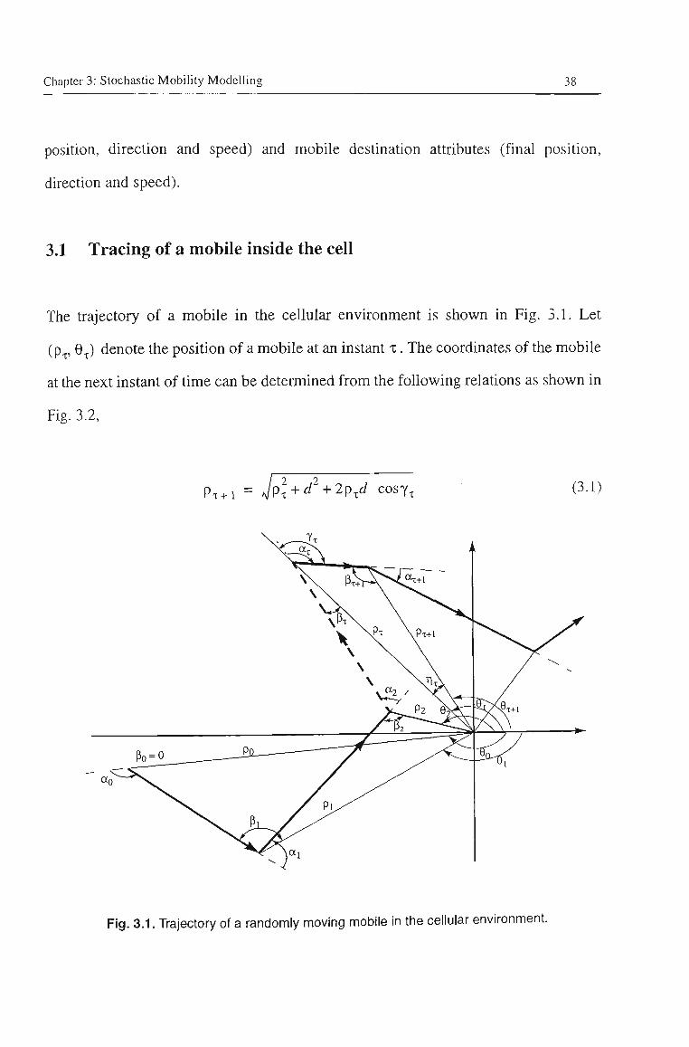
Chapter 3: Stochastic Mobility Modelling 38
position, direction and speed) and mobile destination attributes (final position,
direction and speed).
3.1 Tracing of a mobile inside the cell
The trajectory of a mobile in the cellular environment is shown in Fig. 5.1. Let
(p^, 0 ) denote the position of a mobile at an instant x. The coordinates of the mobile
at the next instant of time can be determined from tiie following relations as shown in
Fig. 3.2,
Pt + i = ^/p^+^^ + 2p^J cosy. (3.1)
Fig. 3.1. Trajectory of a randomly moving mobile in the cellular environment.
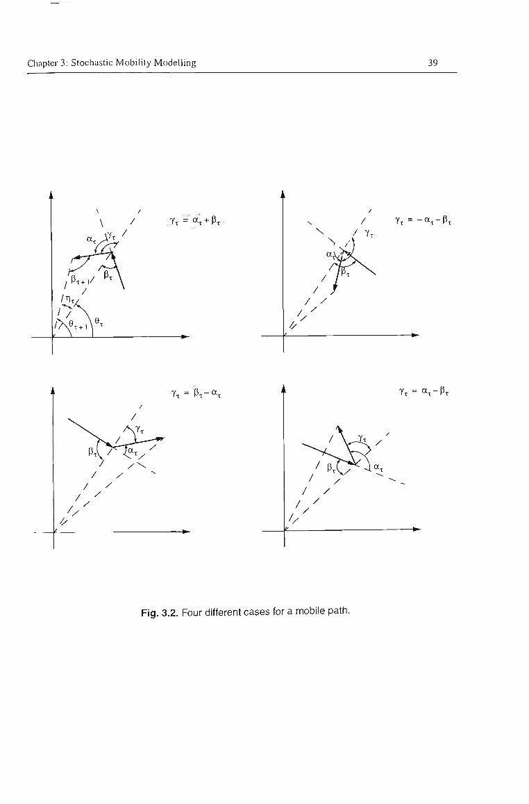
Chapter 3: Stochastic Mobility Modelling 39
N
\ )
«l< 0
/ / / 7
/ /
/ / 7.
^L) Pi. P\ PT ^
/ /
// /
YT = - « T - P T ^
, Yx='Px-«x Yt = « X - P T
Fig. 3.2. Four different cases for a mobile path.
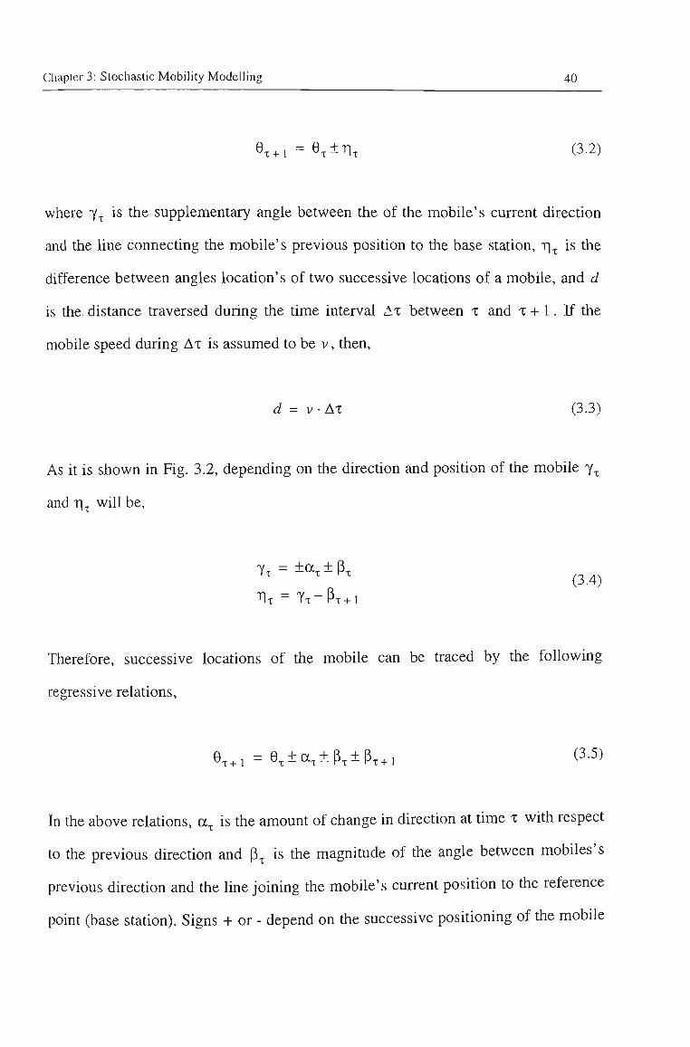
Chapter 3: Stochastic Mobility Modelling 40
0,^1 = 0, ±11, (3.2)
where y, is the supplementary angle between the of the mobile's current direction
and the line connecting the mobile's previous position to the base station, rj, is the
difference between angles location's of two successive locations of a mobile, and d
is the distance traversed during the time interval Ax between x and x + 1. If the
mobile speed during Ax is assumed to be v, then,
d = v•^x (3.3)
As it is shown in Fig. 3.2, depending on the direction and position of the mobile y,
and Tj, will be.
y, = ±a, ± P, " ^ ^ (3.4) "Ht = Yx-Px + i
Therefore, successive locations of the mobile can be traced by the following
regressive relations,
0,^1 = 0 ,±a ,±(3 ,±P ,^ i (3.5)
In the above relations, a, is the amount of change in direction at time x with respect
to the previous direction and P, is the magnitude of the angle between mobiles's
previous direction and the line joining the mobile's current position to the reference
point (base station). Signs + or - depend on the successive positioning of the mobile
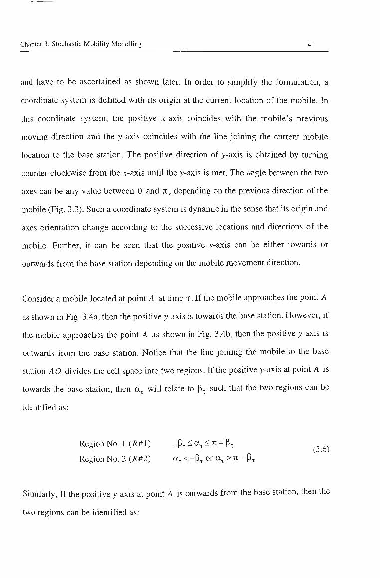
Chapter 3: Stochastic Mobility Modelling 41
and have to be ascertained as shown later. In order to simplify the formulation, a
coordinate system is defined with its origin at the current location of the mobile. In
this coordinate system, the positive x-axis coincides with the mobile's previous
moving direction and the y-axis coincides with the line joining the current mobile
location to the base station. The positive direction of y-axis is obtained by turning
counter clockwise from the x-axis until the y-axis is met. The angle between the two
axes can be any value between 0 and K , depending on the previous direction of the
mobile (Fig. 3.3). Such a coordinate system is dynamic in the sense that its origin and
axes orientation change according to the successive locations and directions of the
mobile. Further, it can be seen that the positive y-axis can be either towards or
outwards from the base station depending on the mobile movement direction.
Consider a mobile located at point A at time x. If the mobile approaches the point A
as shown in Fig. 3.4a, tiien the positive y-axis is towards the base station. However, if
the mobile approaches tiie point A as shown in Fig. 3.4b, then the positive y-axis is
outwards from the base station. Notice that the line joining tiie mobile to tiie base
station AO divides tiie cell space into two regions. If tiie positive y-axis at point A is
towards the base station, tiien a, will relate to (3, such that the two regions can be
identified as:
Region No. 1 (^#1) - P , < a , < 7 r - | 3 , (3.6)
Region No. 2 (P#2) a, < - p , or a., > 7C - P,
Similariy, If tiie positive y-axis at point A is outwards from the base station, then the
two regions can be identified as:
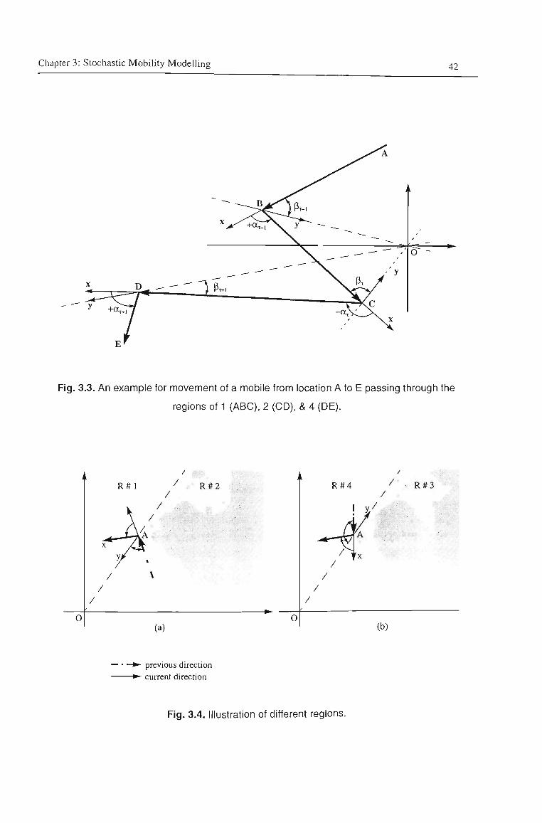
Chapter 3: Stochastic Mobility Modelling 42
Fig, 3.3. An example for movement of a mobile from location A to E passing through the
regions of 1 (ABC), 2 (CD), & 4 (DE).
O
R # l
/
O (a)
R # 4 / •
/ R # 3 •'•
- * - ^ ' 'A
/ I 'X
/
(b)
•>- previous direction ->- current direction
Fig. 3.4. Illustration of different regions.

Chapter 3; Stochastic Mobility Modelling 43
Region No. 3 (/?#3) p ,>a . ,>p , -7C (3 7)
Region No. 4 (/?#4) a , > p, or a , < p , -7 t
Since any value of a. may satisfy one of (3.6) and one of (3.7), to determine a ,
unequivocally, we proceed as follows:
Consider two successive points E and F in the mobile path (Fig. 3.5). Let OF and
OF be the lines joining the base station to the points E and F. Depending on the
directions of the mobile at time x and x - 1, one of the following cases can occur:
[direction => from E to F case I \
[last location => lower side of the line OF
(3.8)
direction => from F to E case II \
last location => lower side of the line OF
direction => from F to E case III \
last location ^> upper side of the line OF
( direction => from E to F
last location ^ upper side of the line OF
Inspection of any of these cases would reveal that the mobile movement is related to
the regional transitions. That is, in case I, the mobile movement is such that it
enters the region R#l at point E. This mobile has the option of moving either to
R#l or to R#2 in continuing its movement at point F. As anotiier example, consider
case II. At point E, the mobile enters the region R#2. At point F it has the option
of moving either to R#3 or to R#4. The same argument could be put in case III
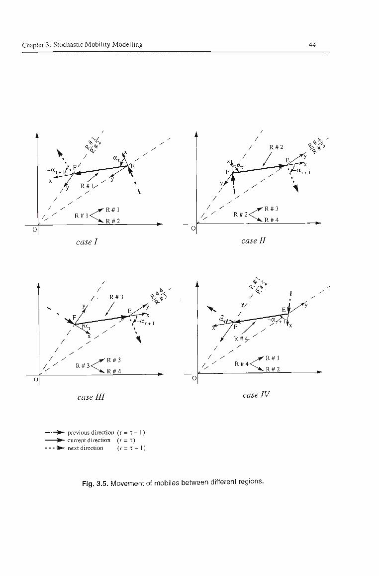
Chapter 3: Stochastic Mobility Modelling 44
O
V
« ^ J . 1
(
/ /
* 5 /
> ^ I ^ ^ — -T^/^ ^ R#l /
« T
y
>x
/ ^ R#i<r
easel
o
/ / <R#
R#
R # 3
4
case II
0 <R#
R #
case III case TV
previous direction (f = x - 1) current direction (r = x) next direction (f = x + 1)
Fig. 3.5. Movement of mobiles between different regions.
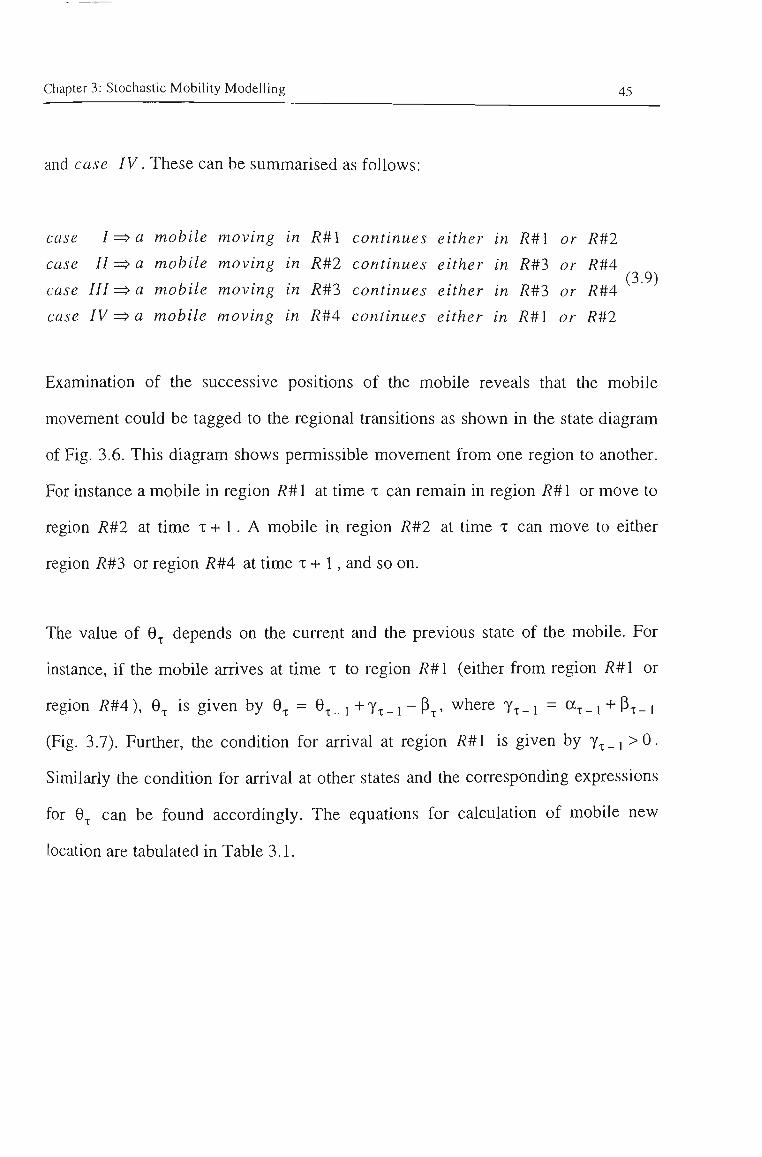
Chapter 3: Stochastic Mobility Modelling 45
and case IV. These can be summarised as follows:
case I => a mobile moving in R#l continues either in R#\ or R#2
case II =^ a mobile moving in R#2 continues either in R#3 or R#4 (3.9)
case III ^^ a mobile moving in R#3 continues either in R#3 or R#4
case IV ^ a mobile moving in R#4 continues either in R#l or R#2
Examination of the successive positions of the mobile reveals that the mobile
movement could be tagged to the regional transitions as shown in the state diagram
of Fig. 3.6. This diagram shows permissible movement from one region to another.
For instance a mobile in region R#l at time x can remain in region i?#l or move to
region R#2 at time x -i- 1. A mobile in region R#2 at time x can move to either
region R#3 or region R#4 at time x -1- 1, and so on.
The value of 0, depends on the current and tiie previous state of the mobile. For
instance, if the mobile arrives at time x to region R#l (either from region R#\ or
region R#4), 0., is given by 0., = 0^_i+y^_i - P,, where y,_i = a ,_ i + P^_i
(Fig. 3.7). Further, the condition for arrival at region R#l is given by y,_i > 0 .
Similarly the condition for arrival at other states and the corresponding expressions
for 0, can be found accordingly. The equations for calculation of mobile new
location are tabulated in Table 3.1.
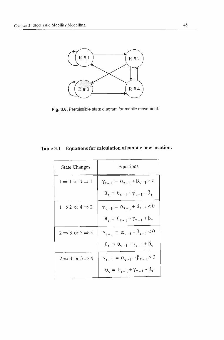
Chapter 3: Stochastic Mobility Modelling 46
Fig. 3.6. Permissible state diagram for mobile movement.
Table 3.1 Equations for calculation of mobile new location.
State Changes
1 => 1 or 4 => 1
1 => 2 or 4 => 2
Equations
y,_i = a ,_ i + P , _ i > 0
ex = Qx-i + Tx- i -Px
Tt - i = ax - i + P t - i < 0
ex = ex - i+Yt - i + Px
2 => 3 or 3 => 3
2 => 4 or 3 =» 4
Yx-i = a , _ , - p , _ , < 0
0, = 0x-l+Yx-l + Px
Yx-i = « X - I - P T - I > 0
0, = O x - i + Y x - i - P t
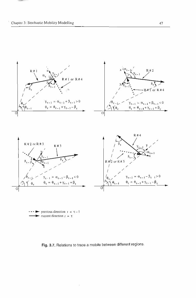
Chapter 3: Stochastic Mobility Modelling 47
;
0
L
R # 1 xy ^ ^
H_,,.^,jtt>C R # 1 or R # 4
/ Q ^ / ^ Y , - I = a t - i + P._i>0
o
R # 2
./>&
^ - f o r R#4
Yt-i = a , _ , + p , _ , < 0
i
0
1,
R # 2 or
Px-l(y
/ /
R # 3
X
/ /
/e ,_^ / Y.-
.^ f e. Qt
R # 3
J-r-^ -—TV-y
1 = a , _ , - P , _ , < 0
= e,_,+Y,_i + P,
o
R # 4
,^^^^9t-i 9. = e,_,4-Y,_,-P,
previous direction t = x-current direction t = x
Fig. 3.7. Relations to trace a mobile between different regions.
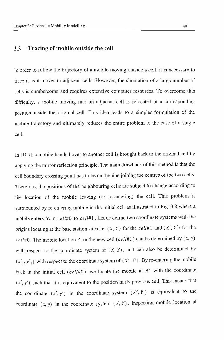
Chapter 3: Stochastic Mobility Modelling 48
3.2 Tracing of mobile outside the cell
In order to follow the trajectory of a mobile moving outside a cell, it is necessary to
trace it as it moves to adjacent cells. However, the simulation of a large number of
cells is cumbersome and requires extensive computer resources. To overcome this
difficulty, gi-inobile moving into an adjacent cell is relocated at a corresponding
position inside the original cell. This idea leads to a simpler formulation of the
mobile trajectory and ultimately reduces the entire problem to the case of a single
cell.
In [103], a mobile handed over to another cell is brought back to the original cell by
applying the mirror reflection principle. The main drawback of this method is that tiie
cell boundary crossing point has to be on the line joining the centres of tiie two cells.
Therefore, the positions of the neighbouring cells are subject to change according to
the location of the mobile leaving (or re-entering) the ceU. This problem is
surmounted by re-entering mobile in the initial cell as illustiated in Fig. 3.8 where a
mobile enters from cell#0 to cell#l. Let us define two coordinate systems with the
origins locating at the base station sites i.e. {X, Y) for tiie cell#l and {X', Y') for the
ceimo. The mobile location A in tiie new cell {celWl) can be determined by (x, y)
with respect to the coordinate system of (X, Y), and can also be determined by
ix',, y',) with respect to the coordinate system of {X', 7') • By re-entering the mobile
back in the initial cell (ce//#0), we locate tiie mobile at A' witii the coordinate
ix\ y') such that it is equivalent to the position in its previous ceU. This means that
the coordinate (jc', y') in the coordinate system {X', Y') is equivalent to the
coordinate {x, y) in the coordinate system (X, Y). Inspecting mobile location at
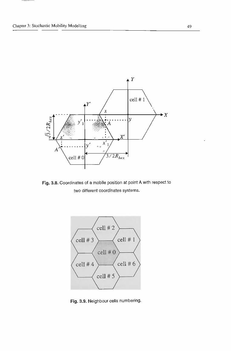
Chapter 3: Stochastic Mobility Modelling 49
Fig. 3.8. Coordinates of a mobile position at point A with respect to
two different coordinates systems.
cell # 2
cell # 3 cell # 1
ceU # 0
cell # 4 cell # 6
ceU # 5
Fig. 3.9. Neighbour cells numbering.
Chapter 3: Stochastic Mobility Modelling 50
points A and A' with respect to the coordinate system {X', Y'), it is possible to
derive the following relations:
X = x\- 3/2Rf^^^
y = y\-j3/2R (3.10)
hex
Depending on the neighbouring cell to which the mobile enters, the mobile's
corresponding location inside the original cell coordinate system {x, y') can be
obtained as follows:
cell No 1
cell No 2
cell No 3
cell No 4
cell No 5
cell No 6
y
y
y
y
y
y'
y
y
y >
y i
y
y'
In order to maintain the appropr:
- j3/2Rf^^^
~ '^^ ^hex
- J3/2R^^^
+ ^/^Rhex
+ ^/3 Rhex
X = x\ - 3/2R^^^
X
X
x'
= X
x\ + 3/2R^^^
x\ + 3/2R^^^
X = X
X I -3/2R^^^
(3.11)
ate direction in the new location, the start angle a.^
of the new direction in the substitute cell should be.
"o = Y + 01-62 (3.12)
where 0,, 02 are tiie location angles of tiie mobile witii respect to the original and
substitute cells respectively, as in Fig. 3.10. This process can be repeated as many
times as needed to keep a mobile inside tiie original cell. The following equations
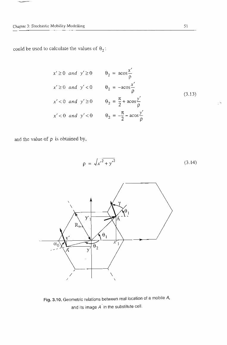
Chapter 3: Stochastic Mobility Modelling 51
could be used to calculate the values of 0o:
x ' > 0 and y'>0 0 2 = acos-
x ' > 0 and / < 0 Oo =
x ' < 0 and y ' > 0 02 =
x ' < 0 and y '< 0 02 =
X -acos —
P K y' - + acos — 2 p 71 y'
acos — 2 p
(3.13)
and the value of p is obtained by.
/ ,2 , ^ p = ^x +y
(3.14)
Fig. 3.10. Geometric relations between real location of a mobile A,
and its image >4'in the substitute cell.
Chapter 3: Stochastic Mobility Modelling 52
3.3 Conclusions
In this Chapter, a mathematical formulation was developed for systematic tracking of
the random movement of a mobile station in a cellular environment. It incorporates
mobility parameters under generalized conditions, so that the model could be tailored
to be applica';.»ie in most cellular systems.The proposed model traces mobiles
systematically in a cellular environment where they are allowed to move in a
quasi-random fashion with assigned degrees of freedom.
Two sets of equations have been derived to trace mobiles locations inside and outside
the cell. These equations enable us to develop a computer simulation program to
investigate the characteristics of different mobility related traffic parameters in a
cellular system.
Chapter 4
Cell Residence Time and Channel
Holding Time Distributions
There are two approaches commonly adopted in the incorporation of mobility in a
cellular system simulation model. The first method, which is used in most
simulations, considers mobility as a subsidiary function in the simulation program.
Examples of this approach can be found in [4, 109, 113, 114, 115]. This method
suffers from the disadvantage that every execution of the simulation requires
mobility modelling. The second approach is to characterise different mobility related
parameters. This method has the advantage that it can be used in analysis as well as in
simulation. A review of the available literature on the characterisation of mobility
related parameters reveals that only a few of the works have dealt with the related
matter in detail, although the need for a comprehensive study is evident. Among
Chapter 4: Cell Residence Time and Channel Holding Time Distributions 54
these works, we can refer to the following.
Guerin [103] has shown that the channel holding time follows a negative exponential
distribution. Morales-Andres et al. [116], and Thomas et al. [107] have used
fluid-flow model of mobility and analytically formulated the cell boundary crossing
rate. PoUini et al. [117] have used these results to calculate the amount of signalling
information needed to deliver calls to mobile stations. Seskar et.al [118] have shown
via simulation that while the model given in [107] provides a good estimate of the
boundary crossing rates for a Manhattan grid of stieets, other conditions lead to
crossing rates larger or smaller than those of the model. El-Hoiydi et al. [119] derive
the probability of crossing the border of a circle and use it to extract the location
update and paging rates. Nanda [49], and Hong et al. [101] have analysed the mean
handover rate. In [108] the mean cell crossings per unit time has been proposed for a
case of three dimensional space.
Among the different mobility-related traffic parameters, one that has not received
sufficient attention so far is user's cell residence time. Therefore, an appropriate
probability distribution that accurately describes the cell residence time remains an
issue to be investigated. A literature survey shows that a relatively few in-depth
papers have been published on this subject and most of these are restricted to simple
mobility situations. Hong and Rappaport [101] have made an elaborate analysis to
obtain the cell residence time probability density function (pdf) for a simplified case
of mobility in which there is no change in speed or direction of the mobile. Further,
in this work the initial speed of the mobile was assumed to follow a uniform
distribution. Del Re, Fantacci and Giambene [102] have assumed that mobiles.
Chapter 4: Cell Residence Time and Channel Holding Time Distributions 55
before crossing a cell, travel a distance uniformly distributed between 0 and 2R^^^,
where R,,^,^ is the hexagonal cell side. They also assume a constant speed witii
uniform distribution and conclude that the pdf of cell residence time is different to
that shown in [101]. Inoue, Morikawa and Mizumachi [120] have apphed the
procedure of [101] for a case of non-uniform speed distribution. However tiiey end
up with a set of unsolved integral equations. Yeung and Nanda [121, 122], Xie and
Kuek [123], Xie and Goodman [124] have shown that contrary to the assumption
made in [101], the speed and direction distributions of the in-cell mobiles are
different from those of the cell-crossing mobiles. They have shown that a more
precise distribution for the speed and direction can be obtained using the Biased
Sampling formula.
While Sanchez Vargas [125], and Lue [126] have assumed cell residence time to be
uniformly distributed over the call duration, Nanda [49], and Lin et. al [127, 128]
have assumed a general distribution for the cell residence time. Malyan, Ng, Leung
and Donaldson [129] have proposed a model where a mobile is positioned initially at
the centre of a circular coverage area and its cell residence time is obtained by using
a two dimensional random walk model. Generally, for the sake of simplicity, in the
absence of any proved probabihty distribution, many authors dealing with the
mobility problem have assumed either explicitly or implicitly, the cell residence time
to be an exponentially distributed random variable [130, 131, 132, 133, 134, 135,
136, 137].
Another important parameter that appears in relation to cellular mobile systems is the
channel holding (or occupancy) time. A knowledge of tiie channel holding time
Chapter 4: Cell Residence Time and Channel Holding Time Distributions 56
probability distribution function is necessary to obtain an accurate analysis of many
teletraffic issues that arise in planning and design of cellular mobile radio systems.
Channel holding time of a cell is defined as the time during which a new or handover
call occupies a channel in the given cell and is dependent on the mobihty of the user.
While this is similar to the call holding time in the fixed telephone network, it is often
a fraction of the total call duration in a cellular mobile network and need not have tiie
same statistical properties. Negative exponential distribution has been assumed to
describe channel holding time in modelling large single cell systems [138, 139, 140].
Guerin [103] has extended tiiis by attempting to describe tiie channel holding tune in
general by the negative exponential distribution.
The outiine of this chapter is as follows. The distribution of tiie cell residence time
for a simplified case (for comparison purposes) and the generalized case is stiidied in
Section 4.1. Based on tiie formulation made in Chapter 3, a computer simulation is
developed to obtain the behaviour of different mobility related parameters. Analysis
of data obtained by simulation is used to show that tiie generalized gamma
distribution function is a good approximation to describe the cell residence time
distribution. Section 4.2 deals with the mean cell residence time. The effect of
changes in direction and speed is analysed and empirical relationships that relate
speed and direction changes to the ceU size are obtained in Section 4.3. In Section
4.4, an expression to determine the average number of handovers in a cell is derived.
In Section 4.5, it is shown that the channel holding time distribution of a cellular
network is a negative exponential function.
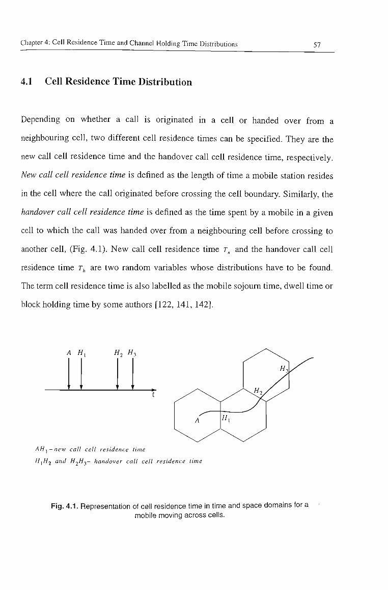
Chapter 4: Cell Residence Time and Channel Holding Time Distributions 57
4.1 Cell Residence Time Distribution
Depending on whether a call is originated in a cell or handed over from a
neighbouring cell, two different cell residence times can be specified. They are the
new call cell residence time and the handover call cell residence time, respectively.
New call cell residence time is defined as the length of time a mobile station resides
in the cell where the call originated before crossing the cell boundary. Similarly, the
handover call cell residence time is defined as the time spent by a mobile in a given
cell to which the call was handed over from a neighbouring cell before crossing to
another cell, (Fig. 4.1). New call cell residence time r„ and the handover call cell
residence time T^ are two random variables whose distributions have to be found.
The term cell residence time is also labelled as the mobile sojourn time, dwell time or
block holding time by some authors [122, 141, 142].
A H
M M
Hi H,
AH^~new call cell residence time
H\H2 and //2W3- handover call cell residence time
Fig. 4.1. Representation of cell residence time in time and space domains for a mobile moving across cells.
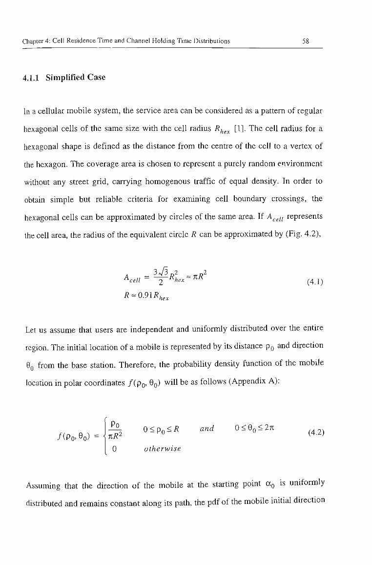
Chapter 4: Cell Residence Time and Channel Holding Time Distributions 58
4.1.1 Simplified Case
In a cellular mobile system, the service area can be considered as a pattem of regular
hexagonal cells of the same size with the cell radius R/^^^ [1]. The cell radius for a
hexagonal shape is defined as the distance from the centre of the cell to a vertex of
the hexagon. The coverage area is chosen to represent a purely random environment
without any street grid, carrying homogenous traffic of equal density. In order to
obtain simple but reliable criteria for examining cell boundary crossings, the
hexagonal cells can be approximated by circles of the same area. If A^^n represents
the cell area, the radius of the equivalent circle R can be approximated by (Fig. 4.2),
^cell = -J-^hex'^'^^ (4 1)
R-0.91R,,,
Let us assume tiiat users are independent and uniformly distributed over the entire
region. The initial location of a mobile is represented by its distance pQ and dkection
OQ from the base station. Therefore, the probability density function of tiie mobile
location in polar coordinates /(pQ, OQ) will be as follows (Appendix A):
/(Po> 0o) = -^^ 0 < P o ^ ^ ^nd O<0o<27r ^42)
0 otherwise
Assuming tiiat tiie direction of tiie mobile at the starting point a^ is uniformly
distributed and remains constant along its path, tiie pdf of the mobile initial direction
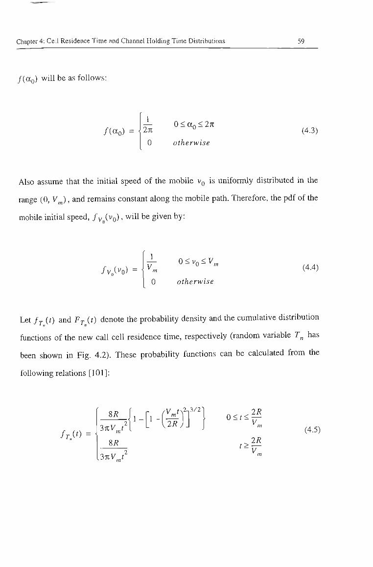
Chapter 4: Cell Residence Time and Channel Holding Time Distributions 59
/(ao) wiU be as follows:
/(cto) = - ^ 0 < an < 271 271 0
0 otherwise
(4.3)
Also assume that the initial speed of the mobile VQ is uniformly distributed m the
range (0, V^), and remains constant along the mobile path. Therefore, the pdf of the
mobile initial speed, fy (VQ) , wiU be given by:
fvS^o) — 0<Vn<V V ^ - ^0 m
m 0
(4.4)
otherwise
Let fr (0 and Fr (0 denote the probability density and tiie cumulative distribution
hinctions of tiie new call cell residence time, respectively (random variable T^ has
been shown in Fig. 4.2). These probability functions can be calculated from tiie
following relations [101]:
fr (0 =
SR
3KVJ'
^ m'- ^
2R
%R
[3nVj
0<t< 2R V.^
(4.5)
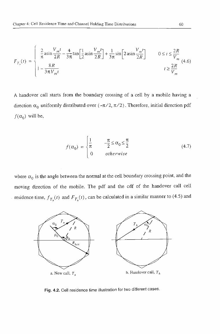
Chapter 4: Cell Residence Time and Channel Holding Time Distributions 60
FT it) =
2 . y,j 4 ^ -asm—-—- r—tan 71 2R 371
8i?
•1 V t-t • m - asm —— 2 2R
+ r—sm 37C
2asm —
3nV,j
O^t^f m
t>^ Vm
(4.6)
A handover call starts from the boundary crossing of a cell by a mobile having a
direction UQ uniformly distributed over (-7c/2,7i;/2). Therefore, initial direction pdf
/(ag) win be,
/(OCn)
I n
0
Ti: , .71 - - < an < -
otherwise
(4.7)
where UQ is the angle between the normal at the cell boundary crossing point, and tiie
moving direction of the mobile. The pdf and the cdf of the handover call cell
residence time, f^ (0 and Fj- {t), can be calculated m a similar manner to (4.5) and
a. New call, T„ b. Handover call, T.
Fig. 4.2. Cell residence time illustration for two different cases.
Chapter 4: Cell Residence Time and Channel Holding Time Distributions 61
(4.6) and is given by.
frit) =
4R
KVJ
_4R__
VnVj
^ m^ ^^ 2R ^<-'<-f
V m
(4.8)
Frft) = i
2 . VJ 2^^ - asm —-— — tan 71 2R n
•1 V tl 1 • m
- asm -—— 2 2R
1 -4R
0 < f < 2R V...
'>-f (4.9)
In [123, 124], it is shown that the speed and direction distributions of tiie in-ceti
mobiles are different from those of the cell-boundary crossing mobiles. Let fv^^i^o)
denote the pdf of the speeds of the in-cell mobiles and fv^^i^o) denote tiie pdf of the
speeds of cell-boundary crossing mobiles. Based on the Biased Sampling [143], it
can be shown that.
/v„(^o) = Vv„(^o)
E[Va] V„^E[V,]
0
0 < V o < V ,
otherwise
(4.10)
where E[VQ] = f v^f {vQ)dvQ is tiie mean speed. Similarly, let / ( ag ) be the pdf J—oo 0
of the directions of all mobile stations, which is uniform m the range (0, 27i:). Based
on the Biased Sampling, the pdf of the directions of the cell-boundary crossing * mobiles, / (ag), can be obtained as:
Chapter 4: Cell Residence Time and Channel Holding Time Distributions 62
* / (OCn) =
1 . . % ^ ^K
-cos(an) - - < a n < -2 " 2 ^ 2 (4.11) 0 otherwise
Equation (4.11) shows that the pdf of the direction of the cell-crossing mobile
stations is not uniform, but has a direction biased towards the normal hue on the
border. Considering (4.10) and (4.11), the relations for fj{t), Fj {t), fj {t) and n n h
Fj (t) could be modified accordingly.
4.1.2 Generalized Case
Eqs. (4.5)-(4.9) represent the new and handover call cell residence tune distributions
for the simplified case of mobility in which there is no change in speed and direction
of the mobile and there is no biasing in speed or direction of the boundary crossing
mobiles. In a general case, the mobility modelhng should include changes in
direction and speed of the mobile. Moreover, it is unrealistic to assume that the speed
is uniformly distributed and remains constant. It is virtually impossible to extend tiie
analysis of the simplified case to cover the general case of mobility. Instead a
simulation approach appears to be the best way out. Based on the mobility model
developed in Chapter 3, a computer simulation program can be developed to study
the mobility under generalised assumptions for different mobility-related parameters.
4.1.2.1 Simulation model
The simulation model is aimed at obtaining statistical estimates of tiie mobile cell
Chapter 4: Cell Residence Time and Channel Holding Time Distributions 63
boundary crossings in a cellular environment in which the mobile is allowed to move
freely with randomly varying velocities and directions within reahstic bounds. In
order that the simulation model be used in a variety of tasks, flexibility is provided in
terms of its inputs and outputs. A simplified flow diagram of the simulation model is
shown in Fig. 4.3. The objective of this simulation is to generate sufficient data to
examine the boundary crossing phenomenon of a mobile as a function of cell size and
mobility-related parameters. This would enable us to obtain the statistical distribution
of the cell residence time and hence that of the channel holding time.
A uniform distribution is assumed for spatial location of the users. This assumption is
valid, since throughout a cellular network, the relative orientation of streets and grids
varies somewhat randomly, giving on the average, a nearly uniform distribution of
possible directions. However, a suitable selection of input parameters allows
modification of this to fit a particular pattem. Since the destination point of mobiles
can be any point in the coverage area, mobiles are allowed to move away from the
starting point in any direction with equal probabihty. Therefore, a uniform
distribution in the range (-7C, K) is suitable for the initial mobile direction.
Depending on the structure of the cellular mobile coverage area, a mobile may move
towards the destination point via different paths. However, in any case, the mobile
direction is biased towards a destination to prevent it from circling around.
In order to make simulation processing time short, array processing is used. For tiiis
purpose, at any given time T , the locations of M mobiles in each of A concentric
cells of radius nR (n= 1, 2, ... A ) can be represented by A x M matrix pair.
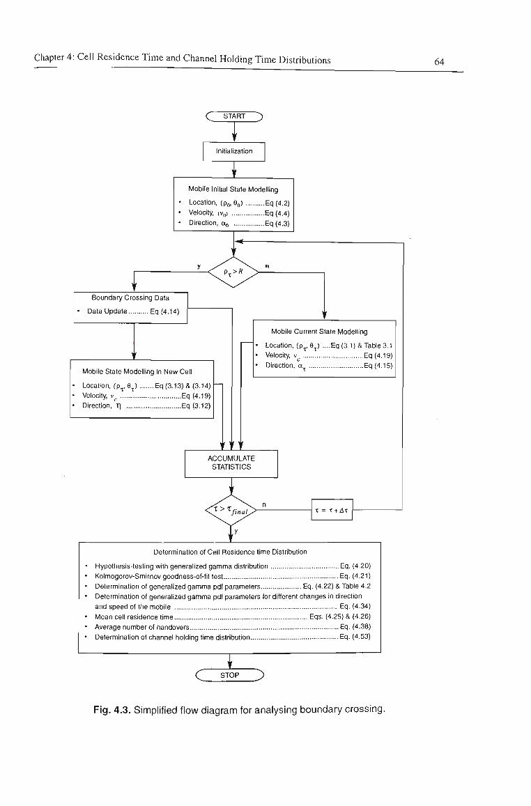
Chapter 4: Cell Residence Time and Channel Holding Time Distributions 64
C START ^
Initialization
Mobile Initial State Modelling
• Location, {p„, e„) Eq (4.2) • Velocity, (v,,) Eq (4.4) • Direction, a„ Eq (4.3)
' ^ P , > « ^ "
Boundary Crossing Data
Data Update Eq (4.14)
Mobile State Modelling in New Cell
Location, (p^, 8^) Eq (3.13) & (3.14) Velocity V Eq (4.19) Direction, r\ Eq (3.12)
: L ] ! J '
Mobile Current State Modelling
Location, (p^, 9 ) ....Eq (3.1) & Table 3.1 Velocity V. Eq(4.19) Direction, a. Eq (4.15)
ACCUMULATE STATISTICS
•t = T + AT
Determination of Cell Residence time Distribution
Hypothesis-testing with generalized gamma distribution Eq. (4.20) Kolmogorov-Smirnov goodness-of-fit test Eq. (4.21) Determination of generalized gamma pdf parameters Eq. (4.22) & Table 4.2 Determination of generalized gamma pdf parameters for different changes in direction and speed of the mobile Eq. (4.34) Mean cell residence time Eqs. (4.25) & (4.26) Average number of handovers Eq. (4.38) Determination of channel holding time distribution Eq. (4.53)
(^ STOP 2^
Fig. 4.3. Simplified flow diagram for analysing boundary crossing.
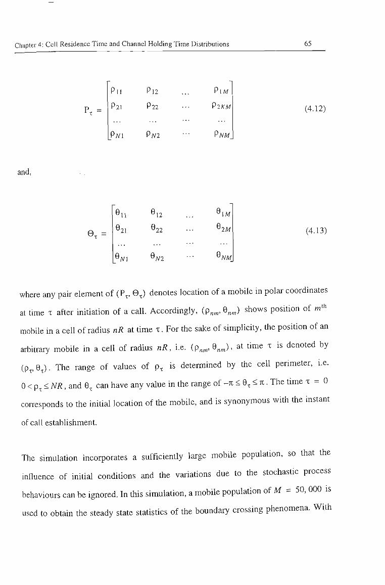
Chapter 4: Cell Residence Time and Channel Holding Time Distributions 65
Px =
P l l
P2I
P;vi
P12
P22
PN2
Piw
PlKM
9NM
(4.12)
and,
0 t =
11
21
0 N\
12
22
0 N2
0 \M
'2M
0 NM
(4.13)
where any pah element of (P„ 0 , ) denotes location of a mobile in polar coordinates
at time x after initiation of a call. Accordingly, (p,^, 0,^) shows position of m*
mobile in a ceU of radius nR at time x. For tiie sake of simphcity, tiie position of an
arbitrary mobile in a cell of radius nR, i.e. (p„^,0„^), at time x is denoted by
(p„ 0,). The range of values of p., is determined by the ceU perimeter, i.e.
0 < p, < A /?, and 0^ can have any value in the range of -71 < 0., < TT . The time x = 0
corresponds to the initial location of the mobile, and is synonymous with the instant
of call estabhshment.
The simulation incorporates a sufficiently large mobile population, so that the
influence of initial conditions and the variations due to the stochastic process
behaviours can be ignored. In tiiis simulation, a mobile population of M = 50, 000 is
used to obtain the steady state statistics of the boundaiy crossing phenomena. With
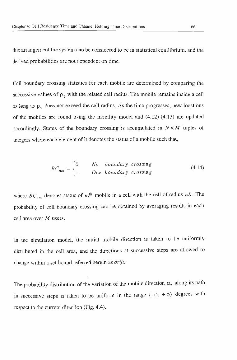
Chapter 4: Cell Residence Time and Channel Holding Time Distributions 66
this arrangement the system can be considered to be in statistical equilibrium, and the
derived probabilities are not dependent on time.
Cell boundary crossing statistics for each mobile are determined by comparing the
successive values of p. with the related cell radius. The mobile remains inside a cell
as k)ng as p. does not exceed the cell radius. As the time progresses, new locations
of the mobiles are found using the mobility model and (4.12)-(4.13) are updated
accordingly. Status of the boundary crossing is accumulated in A x M tuples of
integers where each element of it denotes the status of a mobile such that.
,0 No boundary crossing ,^ , _, 1 One boundary crossing
where EC denotes status of m ^ mobile in a cell with the cell of radius nR. The nm
probability of cell boundary crossing can be obtained by averaging resuhs in each
cell area over M users.
In the simulation model, the initial mobile direction is taken to be uniformly
distributed in the ceU area, and the directions at successive steps are allowed to
change within a set bound referred herein as drift.
The probability distribution of the variation of tiie mobile dkection a^ along its patii
in successive steps is taken to be uniform in tiie range (-(p, -i- (p) degrees with
respect to the current direction (Fig. 4.4).
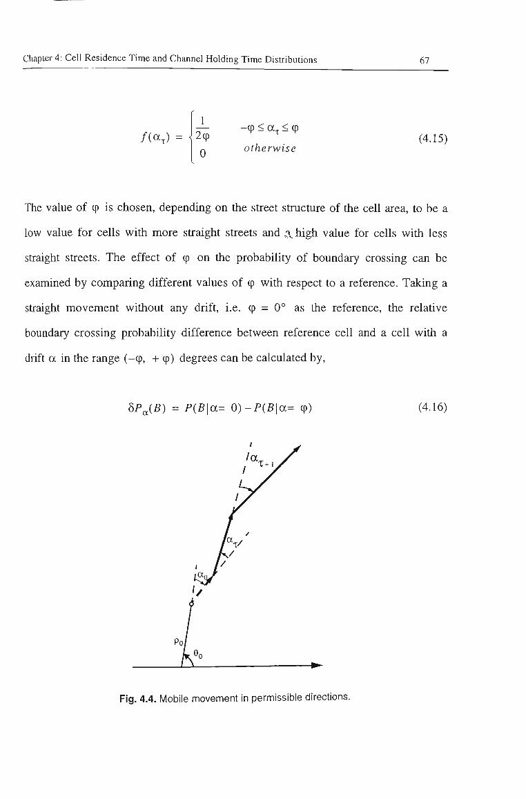
Chapter 4: Cell Residence Time and Channel Holding Time Distributions 67
/ ( a . ) = ^2(p 0
-(p < a. < (p
otherwise (4.15)
The value of (p is chosen, depending on the street stmcture of the cell area, to be a
low value for cells with more straight streets and 3^ high value for cells with less
straight streets. The effect of (p on the probability of boundary crossing can be
examined by comparing different values of (p with respect to a reference. Taking a
straight movement without any drift, i.e. 9 = 0° as the reference, the relative
boundary crossing probability difference between reference cell and a cell with a
drift a in the range (-(p, + (p) degrees can be calculated by.
5P„(5) = P{B\a= 0)-P{B\a= cp) (4.16)
Fig. 4.4. Mobile movement in permissible directions.
Chapter 4: Cell Residence Time and Channel Holding Time Distributions 68
where P{B\a= 0) is the boundary crossing probability in the reference cell, and
P{B\a= (p) is the boundary crossing probability with a drift in the range (-cp, + (p)
degrees.
The initial speed of a mobile station, at the instant the call is initiated, is taken as a
random variable with tmncated Gaussian probability density function, /y^(vo), witii
a mean jx,, and a standard deviation (5^. The choice of such a distiibution seems
reasonable, since the more extreme the speed value, the less likelihood of its
occurrence. Also, it is unlikely that the speed exceeds a certain maximum value.
Therefore if speed is limited in the range [V^-^ = 0, V^^^ = 100 Km/h], the initial
speed of a mobile station pdf will be:
/V„(^0) = 1 G,^/27i
0
Vmin <VQ< Vmax
otherwise
(4.17)
where K is the normalization constant and is given by (Appendix B),
K = J. ' max r^v r
erf erf ^ mill t^v (4.18)
The mobile speed in tiie successive times is a random variable correlated with tiie
previous speed, v^. The current speed, v,, of each mobile is taken to be a uniformly
distributed random variable in tiie range ±10% of tiie previous speed. Therefore the
mobile current speed pdf fyiv^) will be.
Chapter 4: Cell Residence Time and Channel Holding Time Distributions 69
/ v (Vc) = 0.9v <v < l.lv
0.2v^ P ^ P (4.19) 0 otherwise
Any increase in the speed above 100 Km/h is not allowed, and the minimum speed
is taken to be OKm/h.
The speed of the mobile and its dhection are updated at intervals which are
exponentially distributed with an average value of one minute. The motivation for the
choice of an exponential distribution for the length of time between two successive
changes in direction and speed is based on the intuition that the time of the last
change in direction or speed is virtually independent of the time of the next change in
direction. In other words, tiie time distribution between two changes of direction or
speed is assumed memoryless.
In order to check tiie validity of tiie proposed simulation model, a test mn is made for
the simplified case described in Sub-Section 4.1.1 with the same assumptions held.
The probabtiity distribution functions of the new and handover calls' ceh residence
time for this case is calculated using (4.6) and (4.9) and compared with tiie resuhs
obtained by the simulation. As shown in Fig. 4.5 the resuhs obtained by simulation
are in good agreement with the analytical results.
Since the moving direction and the speed of a mobile are non-deterministic
processes, the patii of a mobile will be a random trajectory. Fig. 4.6 shows 5 such
trajectories when drift range is set to be ±20°.
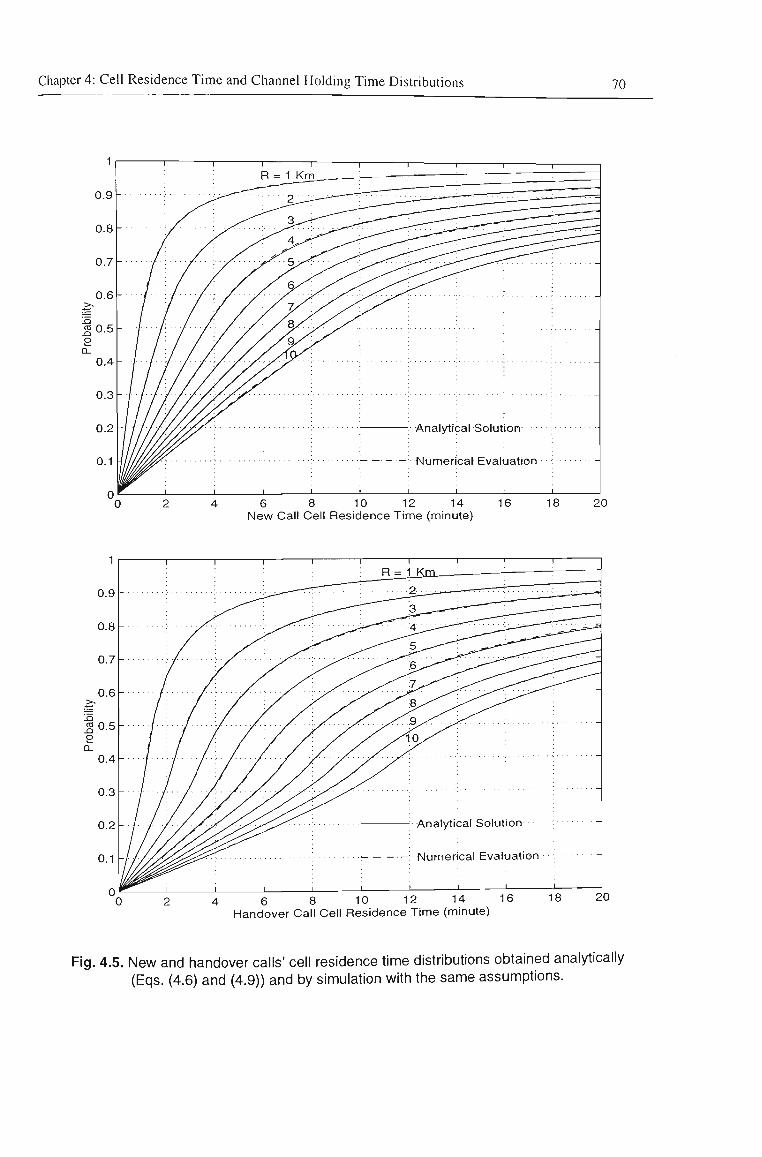
Chapter 4: Cell Residence Time and Channel Holding Time Distributions 70
6 8 10 12 14 New Call Cell Residence Time (minute)
4 6 8 10 12 14 16 Handover Call Cell Residence Time (minute)
18 20
Fig. 4.5. New and handover calls' cell residence time distributions obtained analytically (Eqs. (4.6) and (4.9)) and by simulation with the same assumptions.
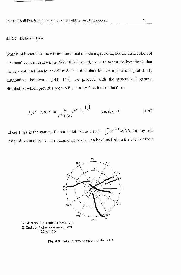
Chapter 4: Cell Residence Time and Channel Holding Time Distributions 71
4.1.2.2 Data analysis
What is of importance here is not the actual mobile trajectories, but the distribution of
the users' cell residence time. With this in mind, we wish to test the hypothesis that
the new call and handover call residence time data follows a particular probabihty
distribution. Following [144, 145], we proceed witii tiie generalized gamma
distribution which provides probability density functions of tiie form:
. , , N C ac-\ \b
fj{t; a,b,c) = — 1 e b r{a)
t,a,b,c>0 (4.20)
where r(a) is the gamma function, defined as r{a) = j {x'' )e ""dx for any real
and positive number a .The parameters a, b, c can be classified on tiie basis of tiiek
S, Start point of mobile movement E, End point of mobile movement
-20<a<+20
270
Fig. 4.6. Paths of five sample mobile users.
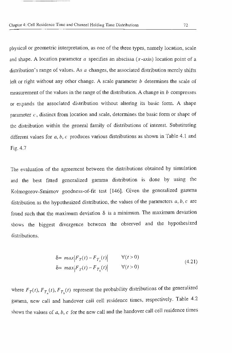
Chapter 4: Cell Residence Time and Channel Holding Time Distributions 72
physical or geometric interpretation, as one of the three types, namely location, scale
and shape. A location parameter a specifies an abscissa (x-axis) location point of a
distribution's range of values. As a changes, the associated distribution merely shifts
left or right without any other change. A scale parameter b determines the scale of
measurement of the values in the range of the distribution. A change in b compresses
or e);pands the associated distribution without altering its basic form. A shape
parameter c, distinct from location and scale, determines the basic form or shape of
the distribution within the general family of distributions of interest. Substituting
different values for a, b, c produces various distributions as shown in Table 4.1 and
Fig. 4.7
The evaluation of the agreement between the distributions obtained by simulation
and the best fitted generalized gamma distribution is done by using tiie
Kolmogorov-Smimov goodness-of-fit test [146]. Given tiie generalized gamma
distribution as the hypothesized distribution, the values of the parameters a, b, c are
found such tiiat the maximum deviation 5 is a minimum. The maximum deviation
shows the biggest divergence between the observed and tiie hypotiiesized
distributions.
h= max\Fj{t)-Fj{t)\ V(r>0)
h= max\Fj{t)-Fj{t)\ V(r>0)
where F^it), Fj {t), F^ (0 represent the probability distributions of tiie generalized
gamma, new call and handover call cell residence times, respectively. Table 4.2
shows the values of a, b, c for the new call and the handover call cell residence times
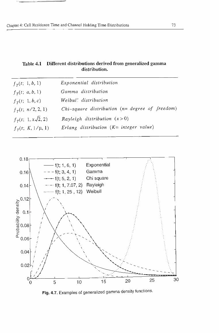
Chapter 4: Cell Residence Time and Channel Holding Time Distributions 73
Table 4.1 Different distributions derived from generalized gamma distribution.
frit
frit
frit
frit
\,b,\) Exponential distribution
a,b,l) Gamma distribution
l,b,c) WeibuV. distribution
n/2 , 2, 1) Chi-square distribution (n= degree of freedom)
l ,x72, 2) Rayleigh distribution (x>0)
K, l / | l , 1) Erlang distribution {K= integer value)
f(t f(t f(t
1, 6, 1) Exponential
3,4,1) Gamma 5,2,1) Chi square
1,7.07,2) Rayleigh 1,25,12) Weibuil
0 5 10 15 20
Fig. 4.7. Examples of generalized gamma density functions.
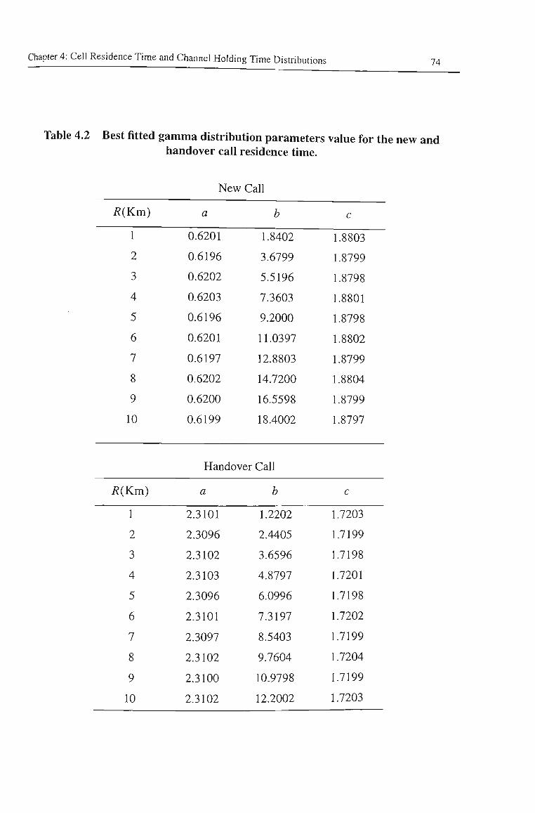
Chapter4: Cell Residence Time and Channel Holding Time Distributions 74
Table 4.2 Best fitted gamma distribution parameters value for the new and handover call residence time.
R{Km)
1
2
3
4
5
6
7
8
9
10
New Call
a
0.6201
0.6196
0.6202
0.6203
0.6196
0.6201
0.6197
0.6202
0.6200
0.6199
b
1.8402
3.6799
5.5196
7.3603
9.2000
11.0397
12.8803
14.7200
16.5598
18.4002
c
1.8803
1.8799
1.8798
1.8801
1.8798
1.8802
1.8799
1.8804
1.8799
1.8797
Handover Call
R{Km)
1
2
3
4
5
6
7
8
9
10
a
2.3101
2.3096
2.3102
2.3103
2.3096
2.3101
2.3097
2.3102
2.3100
2.3102
b
1.2202
2.4405
3.6596
4.8797
6.0996
7.3197
8.5403
9.7604
10.9798
12.2002
c
1.7203
1.7199
1.7198
1.7201
1.7198
1.7202
1.7199
1.7204
1.7199
1.7203
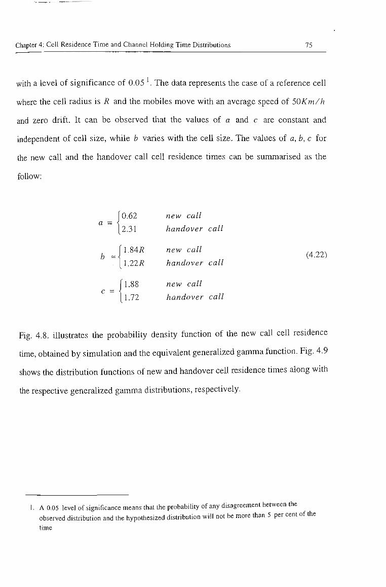
Chapter 4: Cell Residence Time and Channel Holding Time Distributions 75
with a level of significance of 0.05 . The data represents the case of a reference cell
where the cell radius is R and the mobiles move with an average speed of 50Km/h
and zero drift. It can be observed that the values of a and c are constant and
independent of cell size, while b varies with the cell size. The values of a, b, c for
the new call and the handover call cell residence times can be summarised as the
follow:
a = '
b -
c =
jO.62 [2.31
fl.84i?
\l.22R
ri.88 1 1.72
new call
handover
new call
handover
new call
handover
call
call
call
(4.22)
Fig. 4.8. illustrates tiie probability density function of tiie new call ceU residence
time, obtained by simulation and the equivalent generalized gamma function. Fig. 4.9
shows tiie distribution functions of new and handover cell residence times along with
the respective generalized gamma distributions, respectively.
1. A 0.05 level of significance means that the probability of any disagreement between the
observed distribution and the hypothesized distribution will not be more than 5 per cent of the
time
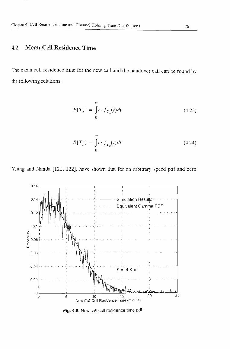
Chapter 4: Cell Residence Time and Channel Holding Time Distributions 76
4.2 JVlean Cell Residence Time
The mean cell residence time for the new call and the handover call can be found by
the following relations:
^[^n] = \t-fTSt)dt (4.23)
E[T^] = lt-fT^(t)dt (4.24)
Yeung and Nanda [121, 122], have shown that for an arbitrary speed pdf and zero
0.16
Simulation Results
Equivalent Gamma PDF
5 10 15 20 New Call! Cell Residence Time (minute)
25
Fig. 4.8. New call cell residence time pdf.
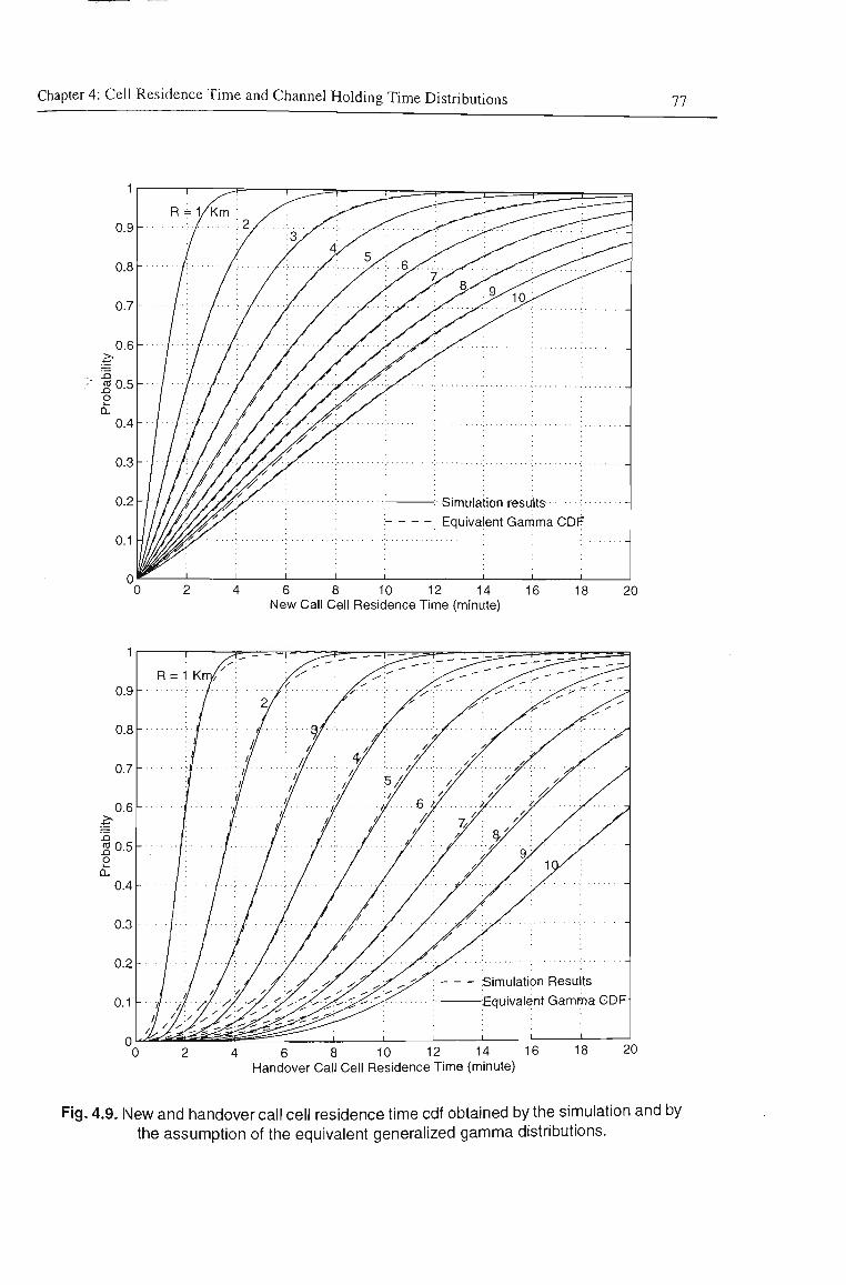
Chapter 4: Cell Residence Time and Channel Holding Time Distributions 77
6 8 10 12 14 New Call Cell Residence Time (minute)
— Simulation Results .Equivalent Gamma GDF
2 4 6 8 10 12 14 16 18 20 Handover Call Cell Residence Time (minute)
Fig. 4.9. New and handover call cell residence time cdf obtained by the simulation and by the assumption of the equivalent generalized gamma distributions.
Chapter 4: Cell Residence Time and Channel Holding Time Distributions 78
drift the mean cell residence time can be obtained by the following equations:
E,r^ , SRE[l/V] ^f^«^ = 3 ^ (4.25)
^t^^l = ^ (4.26)
where R is the cell radius and V is the speed of the mobile in the cell. A comparison
of the results obtained from (4.25)-(4.26) with (4.23)-(4.24) assuming generalized
gamma pdf for f-p {t) and fj. {t) shows that the difference (error) is less than 0.05%
in the case of new calls and 0.015% in the case of handover calls (Table 4.3). This
further justifies the adoption of generahzed gamma distributions to describe the cell
residence times.
4.3 Effect of Change in Direction and Speed
Depending on the street stmcture, a mobile can move in different patiis and may
possess different speeds. The extent of a mobile's change in direction (drift) and
change in speed are the two parameters that govern its mobility pattem. The effect of
mobile direction and/or speed variations on the boundary crossing for different cell
sizes is illustrated in Fig. 4.10. The effect of change in dkection or speed of mobiles
can be considered as equivalent to a change in an average distance travelled or time
spent by a mobile in tiie cell. Thus any increase in a mobile's drift can be tteated as
contributing to an effective increase in the cell radius. Similarly, any increase in
speed of the mobile can be treated as contributing to a decrease in tiie cell residence
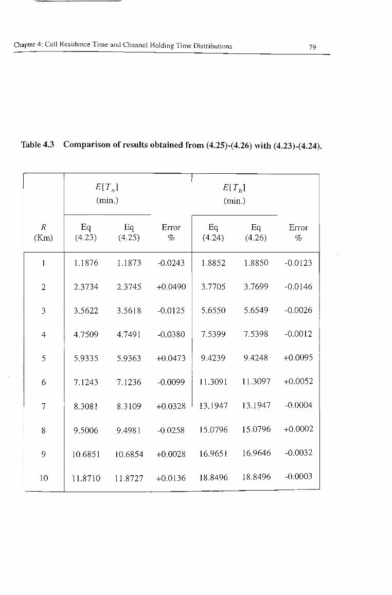
Chapter 4: Cell Residence Time and Channel Holding Time Distributions 79
Table 4.3 Comparison of results obtained from (4.25)-(4.26) with (4.23)-(4.24).
R (Km)
1
2
3
4
5
6
7
8
9
10
EITJ (min.)
Eq (4.23)
1.1876
2.3734
3.5622
4.7509
5.9335
7.1243
8.3081
9.5006
10.6851
11.8710
Eq (4.25)
1.1873
2.3745
3.5618
4.7491
5.9363
7.1236
8.3109
9.4981
10.6854
11.8727
Error %
-0.0243
+0.0490
-0.0125
-0.0380
+0.0473
-0.0099
+0.0328
-0.0258
+0.0028
+0.0136
E[T,] (min.)
Eq (4.24)
1.8852
3.7705
5.6550
7.5399
9.4239
11.3091
13.1947
15.0796
16.9651
18.8496
Eq (4.26)
1.8850
3.7699
5.6549
7.5398
9.4248
11.3097
13.1947
15.0796
16.9646
18.8496
Error %
-0.0123
-0.0146
-0.0026
-0.0012
+0.0095
+0.0052
-0.0004
+0.0002
-0.0032
-0.0003
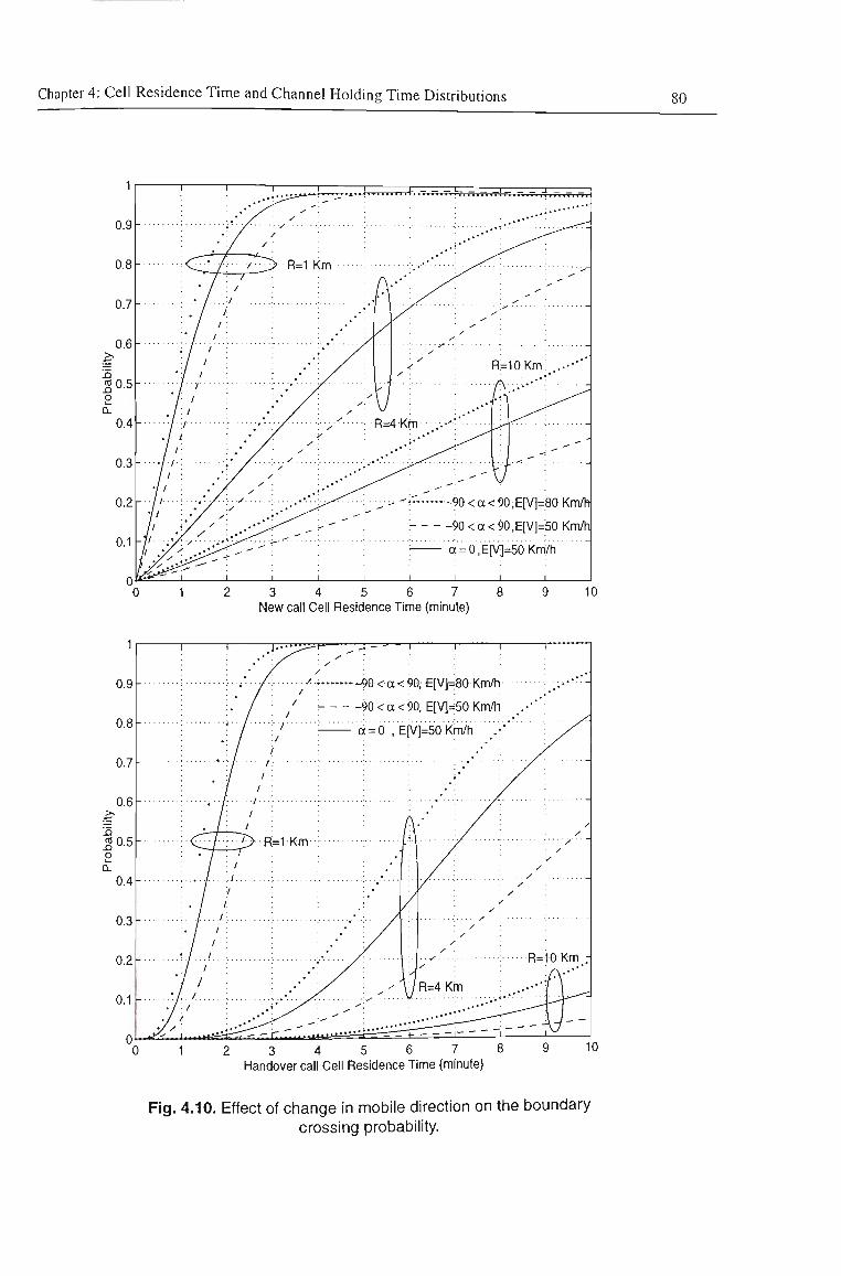
Chapter 4: Cell Residence Time and Channel Holding Time Distributions 80
2 3 4 5 6 7 New call Cell Residence Time (minute)
10
2 3 4 5 6 7 8 9 Handover call Cell Residence Time (minute)
Fig. 4.10. Effect of change in mobile direction on the boundary crossing probability.
Chapter 4: Cell Residence Time and Channel Holding Time Distributions 81
time which can be interpreted as an effective decrease in the cell size. Therefore,
cells with a broad variety of mobility parameters can be replaced by an equivalent
reference cell with an effective radius. The reference cell is defmed as a cell with the
following mobility parameters:
• mobile moves in a straight path, i.e. a = 0° .
• initial speed of a mobile follows a tmncated Gaussian pdf with an average
speed |X = 50 [Km/h] and standard deviation a^ = l5[Km/h].
The main aim is to relate cells with given mobility parameters (i.e. drift a and
average speed [i\) to the reference cell. Two different cases are considered.
case i.) cells in which mobiles move with a drift pdf in the range -(p< a < (p
degrees and speed pdf similar to that of the reference cell. Radius of
such cells is denoted by R^.
case ii.) cells in which mobiles move with zero drift (similar to the reference
cell) and a tmncated Gaussian speed pdf with an average value of
|JL = \i\[Km/h] and a standard deviation of
^ ^ (p^'^_5)/3 [Km/h]. Radius of such cells is denoted by R^.
Consider a cell witii the radius of /?„ having mobility parameters according to case i.
The radius of the equivalent cell 9?„ (which has tiie same residence time but mobility
parameters of the reference cell) is given by:
9t„ = « „ . A « „ (4.27)
Chapter 4: Cell Residence Time and Channel Holding Time Distributions 82
where AR^ is the excess cell radius. Fig. 4.11 shows the excess cell radius for
different drift limits. These curves allow handling of a variety of coverage areas with
different streets orientations and traffic flows by representing those with mobility
equivalent cells with zero drift. The data obtained by simulation satisfies tiie
empirical relation of (4.28) in a least mean square sense.
A/?„ = 0.0038(p/?„ (4.28)
Therefore the equivalent cell radius will be.
^a = KaK (4.29)
where K^ is the proportionality factor and is equal to (0.0038cp + 1).
In the same manner, consider a cell with the radius of R^ and mobility parameters
according to case ii. The radius of an equivalent reference cell 9t^, which has the
same cell residence time but mobility parameters of reference cell is given by:
\ = R. + AR, (4.30)
where AR^ is the excess cell radius. Fig. 4.12 shows the excess ceU radius for
different values of speed obtained by simulation. The data obtained by simulation
satisfies tiie empirical equation of (4.31) in a least mean square sense.
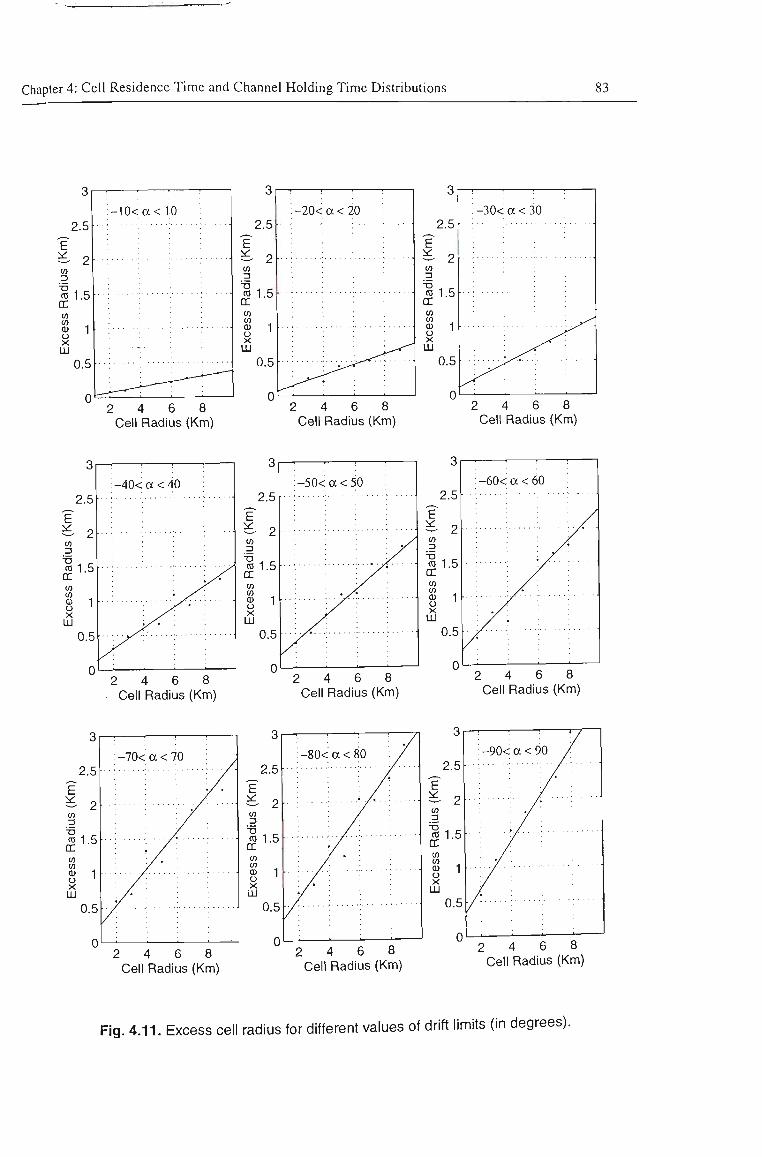
Chapter 4: Cell Residence Time and Channel Holding Time Distributions 83
2.5
^ 2 «
11.5 w (D O X LU
1
0.5
: - 10<a<10
• • - • : •
2 4 6 8 Cell Radius (Km)
2 4 6 8 Cell Radius (Km)
:-30<a<30
2 4 6 8 Cell Radius (Km)
2 4 6 8 Ceil Radius (Km)
2 4 6 8 Cell Radius (Km)
2 4 6 8 Cell Radius (Km)
2 4 6 8 Cell Radius (Km)
2 4 6 8 Cell Radius (Km)
2 4 6 8 Cell Radius (Km)
Fig. 4.11. Excess cell radius for different values of drift limits (in degrees).
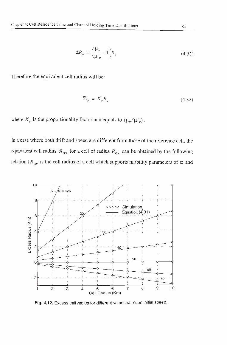
Chapter 4: Cell Residence Time and Channel Holding Time Distributions 84
-^<t^- (4.31)
Therefore the equivalent cell radius will be:
9^v = ^ v ^ v (4.32)
where K^ is the proportionality factor and equals to (p^/p.'^).
In a case where both drift and speed are different from those of tiie reference cell, the
equivalent cell radius 9t„^ for a cell of radius R^^ can be obtained by tiie foUowing
relation {R^^ is the cell radius of a cell which supports mobihty parameters of a and
Fig. 4.12. Excess cell radius for different values of mean initial speed.
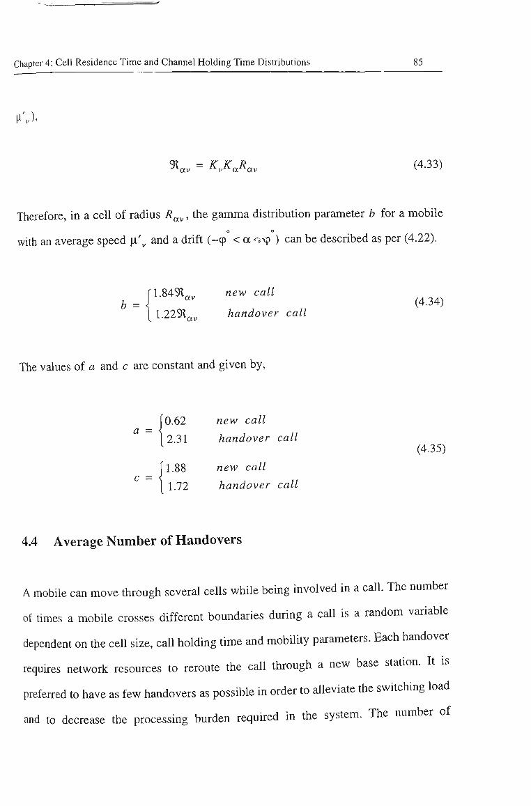
Chapter 4: Cell Residence Time and Channel Holding Time Distributions 85
l 'v)'
9tav = ^ v ^ a ^ a v (4-33)
Therefore, in a cell of radius R^^, the gamma distribution parameter b for a mobile o o
with an average speed \x\ and a drift (-(p < a '*-c? ) can be described as per (4.22).
,T.849t„^ new call b = \ " (4.34)
1.229t(j handover call
The values of a and c are constant and given by.
0.62 new call 2.31 handover call
1.88 new call 1.72 handover call
4.4 Average Number of Handovers
(4.35)
A mobile can move through several cells while being involved in a call. The number
of times a mobile crosses different boundaries during a call is a random variable
dependent on the cell size, call holding time and mobility parameters. Each handover
requires network resources to reroute tiie call through a new base station. It is
preferred to have as few handovers as possible in order to aUeviate tiie switching load
and to decrease tiie processing burden required in the system. The number of
Chapter 4: Cell Residence Time and Channel Holding Time Distributions 86
handovers has a lower bound^ which is equal to the number of boundary crossings a
mobile undergoes. As the number of handovers increases, the handover decision
algorithms need to be enhanced so that the perceived QoS does not deteriorate and
the cellular infrastmcture cost does not skyrocket. In the following sub-sections, we
present two different methods to determine the average number of handovers in a
cellular system.
4.4.1 Method I
The average number of times a non-blocked call is successfully handed over to the
neighbour cell during the call can be obtained from:
E[H] = Y,kProb{H= k} (4.36) k
where Prob{H= k} is the probability that a non-blocked call has k successful
handovers to the successive cells during its life time, and H is an integer random
variable. Let P^ be the probability tiiat a non-blocked new call will require at least
one handover before completion, P;, denote the probability tiiat a non-failed
handover caU wtil require at least one more handover before completion, and P^^ be
the probability tiiat a handover attempt fails. Then [101],
I. Uncertainty in the received signal power due to the fading will make many unnecessary handovers during each boundary crossing. This is explained in Chapter 7.
Chapter 4; Cell Residence Time and Channel Holding Time Distributions 87
Prob{H= 0} = {]-P^) + P^p^^
Prob{H= 1} = Pni^-PFh)(^-Ph + PhPFh)
Prob{H= 2} = Pni^-PFh)Ph(^-PFh)i^-Ph-^PhPFh) (4.37)
Prob{H= k} = Pnil-PFh)iPhi^-PFh)t-\l-P, + P,Pp,)
Substituting (4.37) in (4.36) gives the average number of handovers per call E[H] as
the following:
' 1 = T ^ ^ i ^
Let random variables T^, T^, T^ denote new call residence time, handover call
residence time and the call holding time respectively. From classical teletiaffic
theories it is well known that the call holding time follows negative exponential
distribution, i.e., probability that any randomly selected call holding time will end in
time duration t is.
Fj{t) = 1-e ^'' (4.39)
where E[T^]- 1/p, is the average call holding time.
The value of P., can be obtained as follows:
Chapter 4: Cell Residence Time and Channel Holding Time Distributions
p^^ = Prob{T^>TJ = ^Prob{T^>t\T^ = t} • Prob{T^ = t}dt (4.40) 0
T is mainly dependent on the mobility of the users, and has no influence on the call
duration, T^. Therefore,
oo
p^^ = ^Prob{T^>t}-Prob{T^ = t}dt
0 oo
= j [ l - ^ r , ( 0 ] - / r „ ( 0 ^ ^ ^4.41) 0
e 0
= je"^''-/r„(0^?
Similarly, assuming tiiat call holding time J , has an exponential distribution, tiie
value of P^ can be obtained by the following equation.
P^ = Prob{T^>T^} = \e'^''-frSt)dt (4.42)
0
The values of P„ and P,, can be numerically evaluated by substituting generalized
gamma pdf for f^ (0 and f^ (0 in (4.41)-(4.42) respectively.
4.4.2 Method II
Consider a mobile tiaversing a path with consecutive cell residence times r , 2' • • • ^
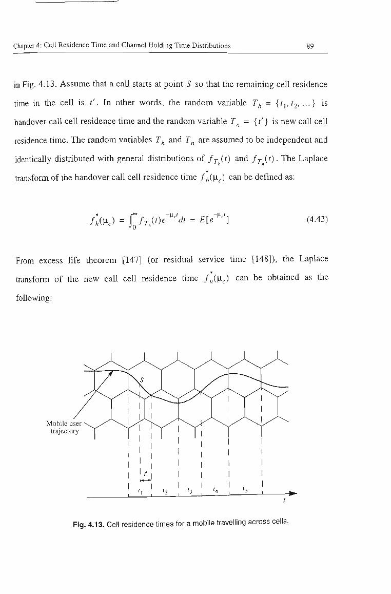
Chapter 4: Cell Residence Time and Channel Holding Time Distributions 89
in Fig. 4.13. Assume that a call starts at point S so that the remaining cell residence
time in the cell is t'. In other words, the random variable P,, = {fj,?2' • ••} is
handover call cell residence time and the random variable T,, = {f'} is new call cell
residence time. The random variables Tf^ and T^ are assumed to be independent and
identically distributed with general distributions of fj- {t) and fj{t). The Laplace *
transform of the handover call cell residence time //,(lic) can be defined as:
-v-ct^ fhi\^c) = \fT,it)' dt = E[e-^'] (4.43)
From excess life tiieorem [147] (or residual service time [148]), the Laplace
transform of tiie new call cell residence time /„(|Xc) can be obtained as tiie
following:
Mobile user trajectory
Fig. 4.13. Cell residence times for a mobile travelling across cells.
Chapter 4: Cell Residence Time and Channel Holding Time Distributions 90
/I(l^c) = r -p!y i [ l - / I (^^c) ] (4-44)
The number of handovers experienced by the call depends on the call holding time
(which is exponentially distributed with mean l/p.^)' and can be obtained as follows
[49]:
/ + h -Ur / + '2 + '3 - M , Z + 'l + h + U -V-c^ , E\H\t',t2,t^,...]=\.\^, ii^e • dx + 2.l^^^ ii^e dx + 3.\^,^^^^^^ \X,e dx^ ...
= Cv^/'''dx^C V^/^^'dx^f iX^e-'^'dx^... (4 .45)
1+e 1+e = e 1 +
Considering E[E[H\t', t^, t^, ...]] = £[^1^'] and using (4.43) we rewrite (4.45) as
follows:
-p,r '
E[H\f] = e'^''[l +/I(M[1 +/;(M[1 + - = -^Z]\^) ^"^'^^^
Taking tiie expectation of (4.46) and considering (4.43) and (4.44), we will have.
E[H] = 1- / , , (M (4.47)
1
h should be noted that (4.47) is only valid for the case of Pp), = 0. Fig. 4.14 shows
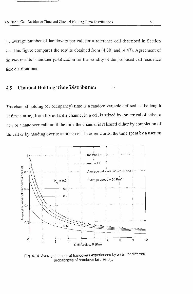
Chapter 4: Cell Residence Time and Channel Holding Time Distributions 91
the average number of handovers per call for a reference cell described in Section
4.3. This figure compares the results obtained from (4.38) and (4.47). Agreement of
the two results is another justification for the validity of the proposed cell residence
time distributions.
4.5 Channel Holding Time Distribution
The channel holding (or occupancy) time is a random variable defined as tiie length
of time starting from the instant a channel in a cell is seized by tiie arrival of either a
new or a handover call, until the time the channel is released either by completion of
the call or by handing over to another cell. In other words, the time spent by a user on
4 5 6 Cell Radius, R (Km)
Fig. 4.14. Average number of handovers experienced by a call for different probabilities of handover failures P^^ .
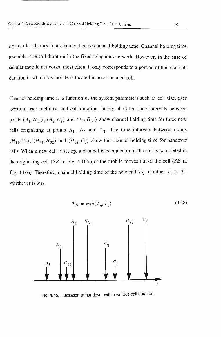
Chapter 4: Cell Residence Time and Channel Holding Time Distributions 92
a particular channel in a given cell is the channel holding time. Channel holdmg time
resembles the call duration in the fixed telephone network. However, in the case of
cellular mobile networks, most often, it only corresponds to a portion of tiie total call
duration in which the mobile is located in an associated cell.
Channel holding time is a function of the system parameters such as cell size, ;iser
location, user mobility, and call duration. In Fig. 4.15 the time intervals between
points (Aj, Hji), (A2, C2) and (A3, H^i) show channel holding time for three new
calls originating at points A^, A2 and A3. The time intervals between points
(//,!, Ci), {H21, H^2^ and (^32, C3) show tiie channel holding time for handover
caUs. When a new call is set up, a channel is occupied until the call is completed in
the originating cell {SB in Fig. 4.16a.) or the mobile moves out of the ceU {SE in
Fig. 4.16a). Therefore, channel holding time of tiie new call T^, is eitiier T„ or T^
whichever is less.
T^ = min{T,^, T^) (4.48)
A.
i u H 11
H 31
t t t f V
C,
i
H 32 C,
Fig. 4.15. Illustration of handover within various call duration.
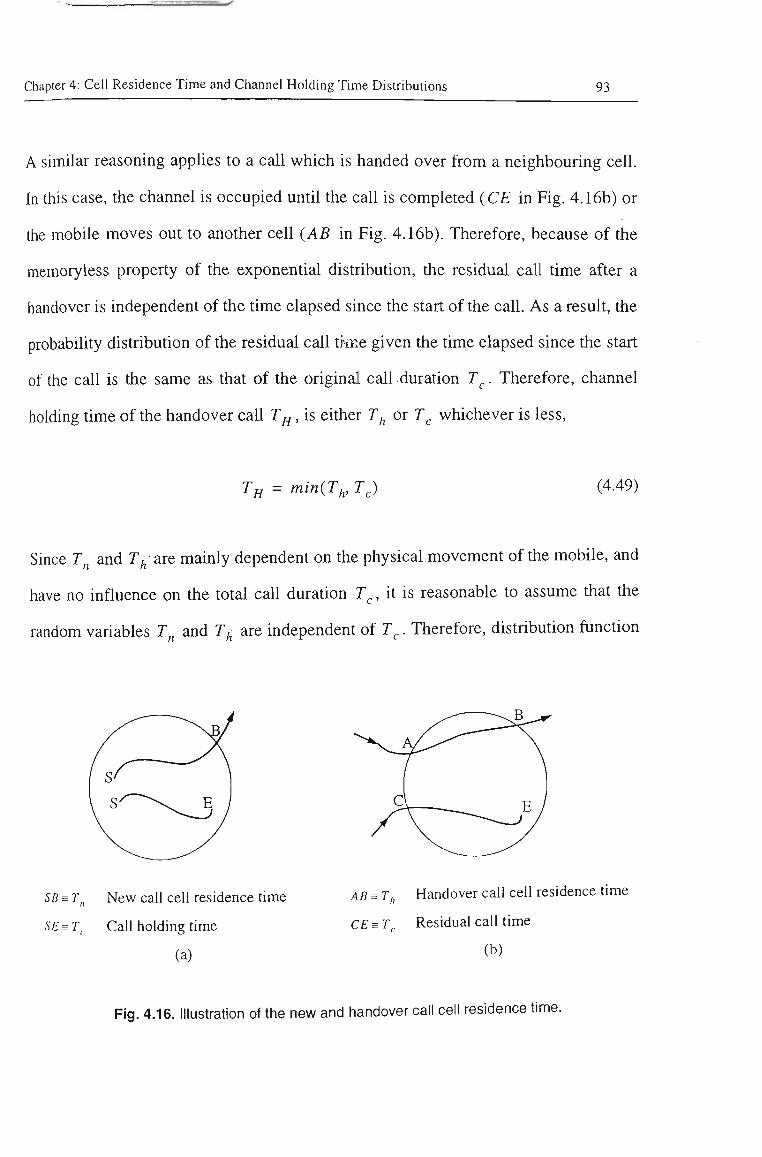
Chapter 4: Cell Residence Time and Channel Holding Time Distributions 93
A similar reasoning applies to a call which is handed over from a neighbouring cell.
In this case, the channel is occupied until the call is completed {CE in Fig. 4.16b) or
the mobile moves out to another cell {AB in Fig. 4.16b). Therefore, because of the
memoryless property of the exponential distribution, the residual call time after a
handover is independent of the time elapsed since the start of the call. As a result, the
probability distribution of the residual call tkiie given the time elapsed since the start
of the call is the same as that of the original call duration T^. Therefore, channel
holding time of the handover call T ^ , is eitiier P , or T^ whichever is less.
Tf^ = min{T,^, P J (4.49)
Since P„ and T^ are mainly dependent on the physical movement of the mobile, and
have no influence on the total call duration P^, it is reasonable to assume tiiat the
random variables P„ and T,^ are independent of P^. Therefore, distribution function
SB = r,, New call ceil residence time
SE = 7-,. Call holding time
(a)
AB = Tf, Handover call cell residence time
CE s T^. Residual call time
(b)
Fig. 4.16. Illustration of the new and handover call cell residence time.
Chapter 4: Cell Residence Time and Channel Holding Time Distributions 94
of the P/y and P/^ can be calculated by (Appendix C):
FT it) = FT it) + FT {t)-FT it)FT (r) " ' " (4.50)
FTSO = FT{t)+FT(t)-FT{t)FT(t)
The distribution of cbannel holding time in a given cell is a weighted function of
F^ it) and P^ {t).lfl is the fraction of tiie average non-blocked new calls out of
average total number of calls in a cell, tiie fraction of the average number of
successful handed over calls will be 1 - ^ . Therefore, tiie distribution function of the
channel holding time including both new and handover calls will be,
P^;0 = ^FTp)^{\-QFT^{t) (4.51)
C can be expressed in terms of the average number of handovers per call E[H] as:
r = \ (4.52) ^ l + £ [ i f ]
Eq. (4.51) can be rewritten in terms of tiie ceU residence time and call holding time
distributions as:
A numerical solution to (4.53), assuming generalized gamma distribution for P„ and
T, indicates tiiat the distribution function of tiie channel holding time in a cell
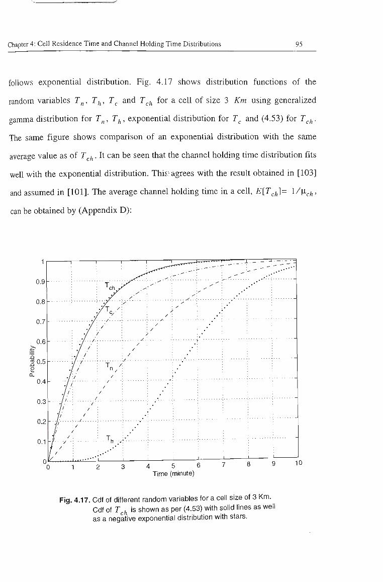
Chapter 4: Cell Residence Time and Channel Holding Time Distributions 95
follows exponential distribution. Fig. 4.17 shows distribution functions of the
random variables P^, P; , T^ and P^^ for a cell of size 3 Km using generalized
gamma distribution for P,,, T^^, exponential distribution for P^ and (4.53) for T^,^.
The same figure shows comparison of an exponential distribution with the same
average value as of T^i^. It can be seen that the channel holding time distribution fits
well with the exponential distribution. This r agrees witii the result obtamed m [103]
and assumed in [101]. The average channel holding time in a cell, E[T^^]= l/li^h'
can be obtained by (Appendix D):
4 5 6 Time (minute)
10
Fig. 4.17. Cdf of different random variables for a cell size of 3 Km. Cdf of T^^ is shown as per (4.53) with solid lines as well as a negative exponential distribution with stars.
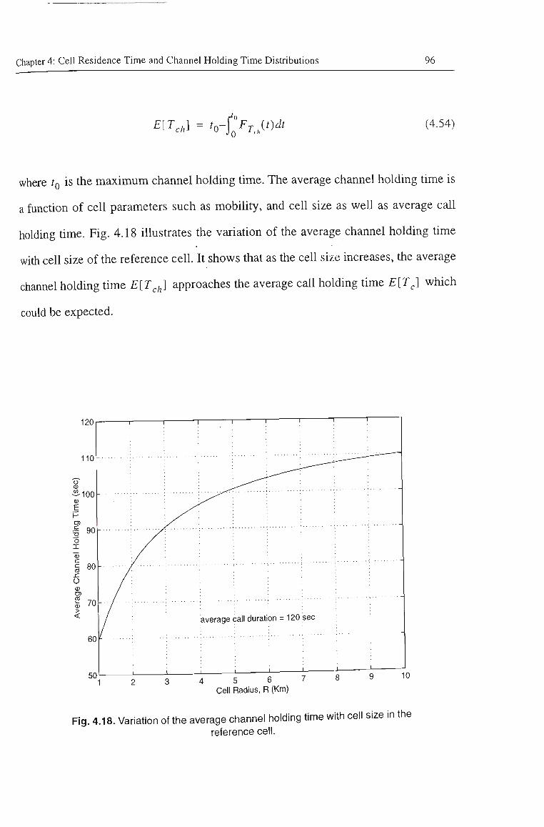
Chapter 4: Cell Residence Time and Channel Holding Time Distributions 96
E[T,,] - t,-f"FTjf)dt (4.54)
where t^ is the maximum channel holding time. The average channel holding time is
a function of cell parameters such as mobihty, and cell size as well as average caU
holding time. Fig. 4.18 illustrates the variation of the average channel holding time
with cell size of the reference cell. It shows that as tiie cell size increases, tiie average
channel holding time E[T^^] approaches the average call holding tune £ [PJ which
could be expected.
120 r
110
sec)
> >
Tim
e( c c
Hol
ding
CD
O
Cha
nnel
00
o
Ave
rage
60
50
1
- • /
1
1 1 1 1 1
y ^ •• ! , , , . . . • • . - ' *.
average call duration = 120
2 3 ' \ 5 ( Cell Radius, R
r 1
; •: -
sec
7 8 9 1
Fig. 4.18. Variation of the average channel holding time with cell size in the reference cell.
Chapter 4: Cell Residence Time and Channel Holding Time Distributions 97
4.6 Conclusions
The mobility model developed in Chapter 3 has been used to characterise different
mobility related traffic parameters in a cellular mobile communication system. These
include the distribution of the cell residence tune of both new and handover calls,
channel holding time and the average number of handovers per call. Results show
that the generalized gamma distribution is adequate to describe tiie cell residence
time distribution of both new and handover calls. It is also shown that the negative
exponential distribution is a good approximation for the channel holding time
distribution in cellular mobile systems.
In order that the results could be made applicable to a wide range of cellular
environments, it was shown that an increase in mobile drift in a cell can be treated as
contributing to an effective increase in the cell radius. Similarly, it was shown that an
increase in the speed of a mobile in a cell can be treated as contributing to a decrease
in the cell size, and vice versa. Taking this excess cell radius into account for
different values of drift and speed, a broad variety of cell coverage areas with
different street orientations and traffic flows can be proportionate to an equivalent
reference cell. Therefore, the distributions for the new call and handover call cell
residence times as well as the channel holding time distribution can be determined for
different cellular environments with various mobility parameters.
Chapter 5
Effect of Handover on the
Teletraffic Performance Criteria
Unlike a fixed network, a cellular network must support mobile customers. In a
cellular mobile communication network, the number of users associated with a base
station at any given time instant is a random variable due to tiie mobile nature of the
users. This inherent feature affects the behaviour of the cellular network in terms of
its offered traffic and requires a new approach for teletraffic performance analysis.
Consideration has to be given to issues such as handover attempt failure, call dropout
and so on. In this Chapter, different radio resource allocation schemes are explained,
a basis for teletraffic performance evaluation is explained, and an analytical model
for teletraffic analysis is described. Also, some traffic policies that give a higher level
of protection to handover calls are analysed, and their effect on the overall traffic
Chapter 5: Effect of Handover on the Teletraffic Performance Criteria 99
performance is assessed. Finally, a teletraffic simulation program which uses the
next-event time-advance approach is described.
The random variables involved in modelling teletraffic in a ceUular network are not
totally amenable to analytical representation. Therefore a simulation procedure based
on next-event time-advance approach couU^be utihzed. This requnes tiie generation
of all attributes of the on-going and up-coming calls in tiie network, by simulation. In
traditional fixed telephone networks, such attributes are confined to tiie call duration
and interarrival time only. However, in a cellular mobile network, a channel could be
occupied by the arrival of a new call or a handover call and it could be released either
by the completion of the call or by handing it to the neighbour cell. Therefore, in
cellular mobile communication networks, other attributes, namely tiie ceU residence
time of both new and handover calls, should also be taken into account, hi Chapter 4,
it has been shown that the cell residence time follows the generalized gamma
distribution in the general case where the movement of users is governed by a set of
random variables. Based on tiiis resuh, a teletraffic model is developed to investigate
the impact of handover on the cellular network performance. In particular it is aimed
at studying how traffic performance is related to different system parameters such as
user mobility and cell size.
5.1 Radio Resource Allocation
Efficient utihzation of tiie radio resource (i.e., spectmm allocated for the cellular
communications) is certainly one of the major challenges in cellular system design.
All of the proposed schemes suggest the reuse of the same radio frequencies in
Chapter 5: Effect of Handover on the Teletraffic Performance Criteria 100
non-interfering cells and have given rise to several channel assignment strategies.
Channel assignment strategies [149] can be classified as fixed (FCA) [4, 150] and
dynamic (DCA) [4, 138, 139, 151, 152]. In between the extremes of fixed and
dynamic channel assignments, there are many possible altematives, such as hybrid
schemes [153, 154], load sharing schemes (including directed retiy [155] and
directed handover [156]) and channel borrowing schemes [149, 157, 158]. These
other schemes are described under flexible channel assignment in tiiis Chapter.
5.1.1 Fixed Channel Assignment (FCA)
In the FCA scheme, each cell has its own distinct channel subset which is different
from the channel subset allocated to its neighbouring cells. The channel subsets are
reused in cells separated by a prescribed distance, called the reuse interval. So, when
a call-in-progress crosses into a new cell, a new channel will have to be found for the
call. If an idle channel is not found, the call-in-progress is terminated abmptly. This
will happen even though there may be vacant channels in adjacent cells. Therefore,
FCA could not attain a high efficiency of total channel usage over the whole service
area if the traffic varies dynamically from cell to cell. However, FCA has the
advantage that it requires a moderate amount of radio equipment in base station and a
simple control algorithm. FCA is superior when traffic demand is high.
5.1.2 Dynamic Channel Assignment (DCA)
I. Channels can be time slots, frequencies, spreading codes or a combination of these
Chapter 5: Effect of Handover on the Teletraffic Performance Criteria 101
At the other extreme is the dynamic channel assignment scheme, where "dynamic"
means that the channels are not preassigned to base stations but are allocated
according to their needs. The dynamic channel assignment implies the lack of a fixed
relationship between cells and channels. In this approach, all channels are kept in a
central pool and allocated to cells as required by tiie real time traffic load. Since it is
not permanently attached to any particular base station, a dynamic channel can float
with the mobile as it moves from cell to cell. The only restriction is tiiat the
cochannel interference constraint should be satisfied. When a mobile moves into a
new cell, the originally-assigned dynamic channel is checked at the new base station
and all base stations within the reuse interval. If the channel passes tiiis check (i.e. it
is not already in use at tiiose stations), it is allowed to continue serving the call.
However, if the original channel is busy elsewhere witiiin a reuse interval of tiie new
base station, a whole new dynamic channel search is undertaken, identical to tiie one
used for new calls. If a substitute channel is not avatiable, tiien the call is terminated.
Such assignment method can significantly increase tiie traffic capacity of tiie
network, especially if serving calls can be assigned new channels according to the
demand arising from new and handover calls.
A particular advantage of dynamic channel assignment is that the system can adapt to
time varying tiaffic requirements. This allows real-time network traffic management
in a cellular network. The disadvantage of dynamic channel assignment is that its
practical implementation requires a great deal of processing power to determine
optimal allocations, and a heavy signalling load on the system to implement all the
channel changes. Among different DCA techniques, tiie Maximum Packing
algorithm introduced by Everitt et al. [159] is of special theoretical interest as it
Chapter 5: Effect of Handover on the Teletraffic Performance Criteria 102
claims to achieve optimum performance. Since this algorithm requires system-wide
information, the complexity of searching all possible re-allocations renders this
strategy hard to implement. While DCA uses channels more efficiently than FCA at
low traffic intensity, it does not show better performance and can even get worse at
high traffic intensity. The reason for this can be explained as follows: Assume that D
is the distance between two cells using the same channel and D^ is the uiinimum
distance necessary to prevent co-channel interference. In the case of FCA, the
channels are assigned to cells in advance so that D equals to D^. In the case of DCA,
since the channels are assigned dynamically on demand, D tends to be greater than
Dj^. This makes the number of tiie reusable channels in DCA less tiian tiiat of FCA,
especially when traffic intensity is high.
5.1.3 Flexible Channel Assignment
In between the extiemes of fixed and dynamic channel assignments, tiiere are many
possible altematives, such as hybrid channel assignment, channel borrowing and
schemes such as durected retiy and directed handover, which take advantage of tiie
fact that some percentage of the mobiles may be able to obtain sufficient signal
quality from two or more cells. With the hybrid scheme, one subset of channels is
fixed and the rest is kept in a common pool. This scheme is meant to gain advantages
of both fixed and dynamic channel assignments.
In most systems tiie mobiles are always connected to tiie base station to which they
receive the strongest received signal. However, in some situations the utilization of
the spectrum can be improved if mobiles are permitted to use base stations besides
Chapter 5: Effect of Handover on the Teletraffic Performance Criteria 103
the strongest. In fact, this happens mostiy in the overlap area where received signal
strength from different base stations could be enough to be connected. Based on tiiis,
Eklundh has proposed a variation of FCA called directed retry. In tiiis approach, if
the base station with the highest signal power can not accommodate another call, the
mobile with the new call has the opportunity to establish a connection witii the base
station with the second highest power. Directed retry preserves the metrics of the
FCA and at the same time, reduces the blocking probability of a ceU by increasing its
channel utilization. The improvement is accomplished at the expense of an increased
number of handovers and an increased level of cochannel interference. A traffic
analysis of directed retry can be found in [160]. In [156], the scheme was enhanced in
a way that both on-going calls and new calls were allowed to be redirected to another
base station. Hence, the tiaffic load is shared among the base stations and the
blocking probabihty is decreased. This method is called directed handover. The
disadvantage with these load sharing methods (i.e. directed reti^ and directed
handover) is that if a mobile does not use the base station witii tiie highest signal
power it becomes more sensitive to interference.
During the operation of a cellular system, unexpected growtii of traffic may develop
in various cells and create traffic congestions. Therefore, a metiiod which is adaptive
to such a change will improve the capacity efficiency. Channel borrowing scheme is
known to be a viable solution to alleviate congestions. In this method all channels are
nominally pre-ahocated to tiie base stations (same as FCA), but may be borrowed on
demand by other base stations.
Lin, Noerpel and Harasty [161] recently have proposed a new channel assignment
Chapter 5: Effect of Handover on the Teletraffic Performance Criteria 104
scheme called sub-rating scheme (SRS) that creates a new channel on a blocked base
station for a handover access attempt by sub-rating an existing call. Sub-rating means
an occupied full-rate channel is temporarily divided into two channels at half the
original rate: one to serve the existing call and the other to serve the handover
request.
5.2 Teletraffic Performance Parameters
The teletiaffic performance can be assessed in terms of the grade of service, the
traffic carried by the network, tiie channel utilisation, and the spectmm efficiency.
The grade of service is defined as any practical interpretation of a congestion
function [162]. In a fixed network, this parameter refers to the probabihty that a call
trying to access the system is denied because of channel unavailability. However, in
the case of a cellular network, because of its unique features, tiiis simple definition is
insufficient, and the grade of service (GoS) is defined to include a combination of tiie
following probabilities.
5.2.1 Setup channel blocking probability
In a cellular network, a control channel is often allocated exclusively for setting-up
the calls. When a mobile attempts to make a call, it accesses tiie network fhrst tiuough
the setup channel. The setup channel may handle tiie arriving tiaffic on a delay basis
or on a loss basis. For the delay case, tiie call setup delay can be calculated using tiie
Erlang C formula. For tiie loss case, tiie setup channel may be of ALOHA type with a
collision probability, or of blocked-calls-cleared (BCC) type discipline witii tiie
Chapter 5: Effect of Handover on the Teletraffic Performance Criteria 105
probability of loss P^^ calculated according to the Erlang B formula.
5.2.2 New call blocking probability
If the setup channel is free, the mobile station transmits a seizure message requesting
a voice radio channel. The new call blocking probability Pg^ rep.resents the
probability that a call attempt which succeeds in accessing the setup channel fails to
access the network because of the unavailability of a free radio channel. This
probability can be defined as:
Pg^ = Prob{a new call arrives in a cell when all channels are occupied}
_ number of new calls fail to obtain a channel C-^- i ; number of new call attempts
5.2.3 Fixed network blocking probability
Most of tiie mobile calls pass through tiie fixed network. Therefore, any blocking due
to unavailability of link through the fixed network affects tiie GOS of the mobile
radio network. It is usually assumed that the blocking probability of the fixed
network Pg; is much smaller than tiiat of the cellular network due to the limited
availability of the mobile radio channels. For the mobile to mobile call, tiie fixed
network may not be involved (if they are in the same cell), and hence its reliability
does not affect the GOS. In tiiis situation, the fixed network blockmg probability is
replaced by the probability of blocking of the radio channel in the otiier ceU witiiin
which the called party is reached.
Chapter 5: Effect of Handover on the Teletraffic Performance Criteria 106
5.2.4 Handover attempt failure probability
A distinct feature of cellular networks is the handover where a mobile crossing its
cell boundary during a call needs to be allocated a new channel in a new cell. The
probability that this reallocation cannot be achieved is referred to as handover call
blocking, or handover attempt failure probability, Pp^^. The handover failure
probability represents the proportion of handover requests which are blocked during
handover request. This parameter can be defined as:
Pph ~ P''oZ?{ahandover call arrives when all channels are occupied}
_ number of handover calls fail to obtain a channel \.~>.l) number of handover call attempts
Handover failure probability is a good performance measure, because it reflects on
the number of boundary crossings and hence the mobility of the mobile.
5.2.5 Dropout probability
The probability that a call will be dropped out during a call is anotiier measure of
traffic performance. This may arise either due to insufficient signal strength tiuough
fading of the radio signal, or through an unsuccessful handover attempt. Even if one
neglects the dropout through signal fading, the probability of dropout is different
from the handover blocking probability, because a mobile may cross several cell
boundaries successfully before striking a boundary where it is blocked. The dropout
probability P^ is defined as tiie probability that a non-blocked new call will be
dropped out at some point during a call, while the handover blocking probabihty is
SBSaSBDBai
Chapter 5: Effect of Handover on the Teletraffic Performance Criteria 107
simply the same measure per cell boundary crossing. A forced termination (i.e.
dropout) can be preceded by several successful handovers. Therefore,
P^ = Pro^{Forced termination of a call due to a handover failure}
_ fc number of calls forced to terminate \->-3) number of the non blocked new call attempts
A fraction of the new calls which are not blocked will eventually be forced into
termination if it succeeds in each of the first (/ - 1) handover attempts, but fails on
the Ith handover attempt, i.e..
P^= \Prob{{l-l)successful handover} • Prob{l th handover fails} {5.4)
1= 1
where,
Prob{{l-l)successful handover} = P ni"^ - P Fh) ' h^"^ ~ ^ Fh^ Phi^'^Fh)
= P,,-P[-'-{^-PFht'
and,
Prob{l th handover fails} = Ph'PFh ^ ^^
where P„ is tiie probability tiiat a non-blocked new call will require at least one
Chapter 5: Effect of Handover on the Teletraffic Performance Criteria 1 Qg
handover before completion, and P,^ denotes the probability tiiat a non-failed
handover call will require another handover before completion. Hence:
(5.7) ^Fh^n
^-(^-PFh)Ph
5.2.6 Unsuccessful call probability
Assuming that setup channel and fixed network blocking probabilities are negligible,
the probability of an unsuccessful call P^ is the probability that a call is not
completely served due to either the initial blocking of the call attempt or the failure of
a subsequent handover request. Therefore, P^^ is the sum of the probabilities of
blocking at the start of the call and dropping out afterwards and could be obtained by,
Pu = PBn + PD(^-PBn) (5-8)
5.3 Teletraffic Analysis
Due to the occurrence of handover and forced call termination, the simple Erlang loss
formulas or other product form solutions cannot be applied dhectiy in cellular
systems [132, 163]. To clarify tiiis point. Fig. 5.1 shows tiie Markov chain reflecting
traffic in two isolated adjacent cells with each cell supporting up to n simultaneous
calls. A state of tiie system is shown by (n,, ^2), where n^ is the number of calls in
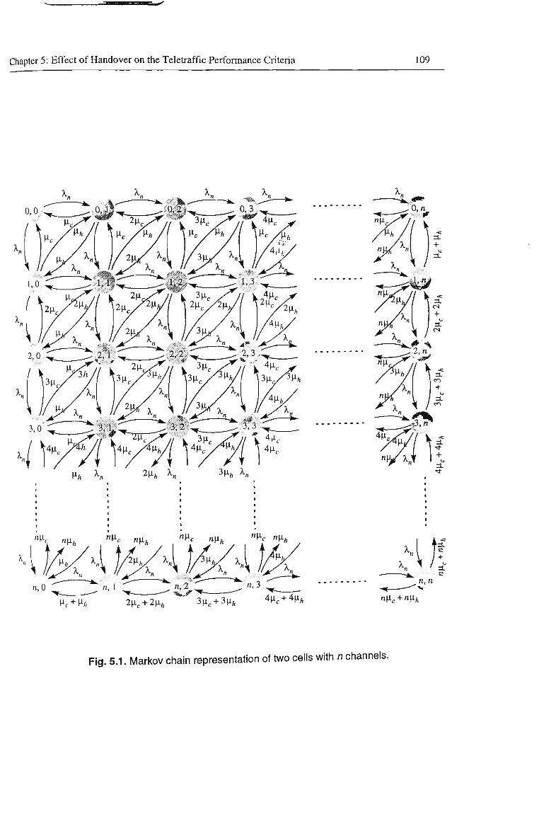
Chapter 5: Effect of Handover on the Teletraffic Performance Criteria 109
H K '^^h K '^^h K
'V. „p,, Wc njift « c nfl^ "M-c nn^
. ^ , H'
nit^ + «Hft
Fig. 5.1. Markov chain representation of two cells with n channels.
Chapter 5: Effect of Handover on the Teletraffic Performance Criteria 110
progress in cell 1 and nj is the number of calls in progress in cell 2. Let p^ and \i^ be
the call completion rate and handover rate respectively per cell. The transition rates
from state (nj, n2) to state (n, - 1, n2) and from state (nj, nf) to state (nj, n2- 1)
are given by njix^ and n2|i^ respectively. However, the transition rates for the
boundary states where n^ = n or nj = n are given by n^{\i^ + \if^) and n2(M c + V^h)
respectively. Only when M-j = 0 (which coEEesponds to a system without handovers
such as a fixed telephone network), the equilibrium state distribution has a product
form solution given by:
p{n^,nf) = PQ O r o
n,! n y^rjy-i-j
(5.9)
where /?(«,, n2) represents tiie steady state probability of having n^ calls in cell 1
and 72 calls in cell 2. Here, p^ is the normalization constant, and p^ is tiie offered
traffic in the network given by p„ = \/[i,, where X^ is the average new call arrival
rate per cell. However, if tiie number of handovers is not negligible, tiie exact steady
state distribution does not have a product form solution. In tiiis case, analytical
modelling can be performed using the following approximation.
Let the arrival of calls to a cell consist of the newly initiated calls witiiin the cell (new
calls) and the calls handed over from tiie neighbouring cells (handover caUs).
Assuming that botii new and handover call arrivals are Poisson processes witii
average call arrival rates X^ and X^^, respectively, tiie total call arrival rate X, per cell
will be tiie superposition of the two Poissonian streams such that.
Chapter 5: Effect of Handover on the Teletraffic Performance Criteria i l l
Xj = X^ + X^ (5.10)
Considering the fact that superposition of the two Poissonian streams is also a
Poisson process, the total call arrival rate will be a Poisson process. A channel
completion time (the length of time that a call remains in a cell) is determined by the
time the channel becomes free after a call completion or a call handed over to another
cell. Therefore, the total channel service rate \i^f^ will be the sum of tiie call
completion rate p, and the call handover rate p. .
\^ch = \^c + H ( - ^
Hence, tiie total effective traffic intensity in a cell due to new and handover calls will
be:
P. = h^V^ch (5-12)
Let Pg be the overall blocking probability in a cell. Then, the total departure rate of
calls from the cell is ?ij( 1 - P^). Therefore,
. -^(X^P i _ i ^ (5-13)
where |i;,/(ii^ + ^i,) is tiie probability tiiat a call will hand over to neighbour cell,
otherwise it will terminate inside tiie cell. Rearrangement of (5.13) will resuh in:
Chapter 5; Effect of Handover on the Teletraffic Performance Criteria 112
From (5.11)-(5.14), after some algebraic manipulation, tiie effective offered traffic
p , can be found as,
Pe = K^(\^C + HPB) (5.15)
If the product of the average call holding time and the average velocity of a mobile is
small compared to the cell size (i.e., v/p,^ « R), the probability of the mobile crossing
a cell boundary during a call is low. In this case, the probability of new call blocking
is the major indication of system traffic performance and the offered traffic to a cell
in the absence of any handover calls will simply be X^/\i^. Any decrease in cell size
results in an increase in the handover rate resulting an increase in handover blocking
probability. A premature call termination due to failure during handover forces the
mean effective call duration to decrease (or call departure rate to increase). In order
to make the system in Fig. 5.1 reversible and to take the overall call blocking
probability Pg into account, it is assumed that the effective call duration of a new
caU is exponentially distributed with mean l/p.^, where p^ = p^ + ji^jP^.
In the case where there is no assigned priority to handover calls, a handover call
entering a cell requires a channel in tiie new cell just as a call originating in the cell
does. Hence, tiie same fraction of either category of calls will be unsuccessful. That
is, the blocking probability of a new call Pg^, the failure probability of a handover
call P / , and the overall call blocking probability PQ will be the same and can be
Chapter 5: Effect of Handover on the Teletraffic Performance Criteria 113
found using Erlang-B formula as per (5.16),
P?/C! PB= PBn= PFh = -¥ (5.16)
I P>-( = 0
where C is the number of channels allocated to a cell. Equation (5.16) should be
solved iteratively, since p^ is related to the blocking probabihty.
5.4 Handover Prioritization Schemes
When all channels assigned to a cell are occupied, any handover attempt to tiiat cell
will be blocked, causing a forced termmation of tiie call in progress. Such an
intermption is perceived as more annoying to a user tiian a failure to set up a new call
which only contributes to a delay in estabhshing a communication link. It is tiierefore
necessary to estabhsh traffic policies that minimize the probability of forced
termination of calls in progress due to handover failures, while not penalizing the
new calls too much. The probability of handover call failure can be decreased by
giving some form of priority to handover requests over the new call attempts. Two
generic handover prioritization schemes have been proposed and studied to reduce
the dropout probability, namely:
• Reserved channel scheme [101, 164],
• Queueing prioritization schemes [101, 127, 165, 166].
Chapter 5: Effect of Handover on the Teletraffic Performance Criteria 114
Other prioritization schemes can be viewed as variations of the above. Handover
prioritization schemes, in general, result in a decrease in handover failures and an
increase in new call blocking which, in turn, reduces total carried traffic.
5.4.1 Reserved channel scheme
In the reserved channel scheme, a fixed or dynamicaUy adjustable number of channels
are exclusively reserved for handover requests. These channels are not available for
setting up new calls and therefore the probability of a blocked new call will increase, but
this may be the price we are willing to pay for a reliable handover. Let C;, be the number
of reserved channels among the C available channels per cell reserved to protect
handover calls, and the remaining C-Cf^ channels are shared by both new calls and
handover calls. The aim is to determine an appropriate value for C^ in order to protect
handover calls from excessive blocking without unduly increasing the blocking of new
calls. The total call arrival rate in a cell X, is equal to X„ -i- Xf^ if the number of calls
present in the system is less than C-Cf^, and X,^ if there are C-Cf^ calls or more in the
system. At statistical-equilibrium, the probability of finding / busy channels can be
calculated using basic queueing theory [148, 167] as.
P{i)=
i
^P(O) /= 1,2, . . . , C - C , (5.17)
c-c„ i-iC-C,) Pe Ph p^Q^ i= C-Cf^+l,...,C
ll
where, p , = X,/\i^^, p , = {X,^ + X,^)/{\i, + \ih) and P(0) is merely a normalizing
Chapter 5: Effect of Handover on the Teletraffic Performance Criteria
factor so that the state probabilities add up to 1, i.e.,
115
P(0) = 1 C-C,k
V^ He C-C
k = 0 k\
c
' s k = C-C^+\
k-iC-C,) Ph
k\
(5.18)
Therefore, the new call blocking and handover failure probabilities can be obtahied
by,
Ps^ = Prob{i>C-C,)= X ^(^•) i^C-C,
Pp^ = Prob{i>C) = P{C)
(5.19)
I.e.,
PBn -
C / - ( C - C , ) - , C-C, ^ Ph
Pe L — i= C-Cu
ll P(0)
C-C, c,
Fh C!
(5.20)
h is clear that when C;, = 0, P^^ = Pp^- Evaluation of the two blocking
probabilities in (5.20) as illustrated in Fig. 5.2 reveals that the rates of change of two
blocking probabilities are different. This imphes that the decrease in blocking
probability of handover calls witii increasing number of reserved channels is greater
than tiie corresponding increase in the blocking probability of new calls. This is what
makes the reserved channel scheme useful.
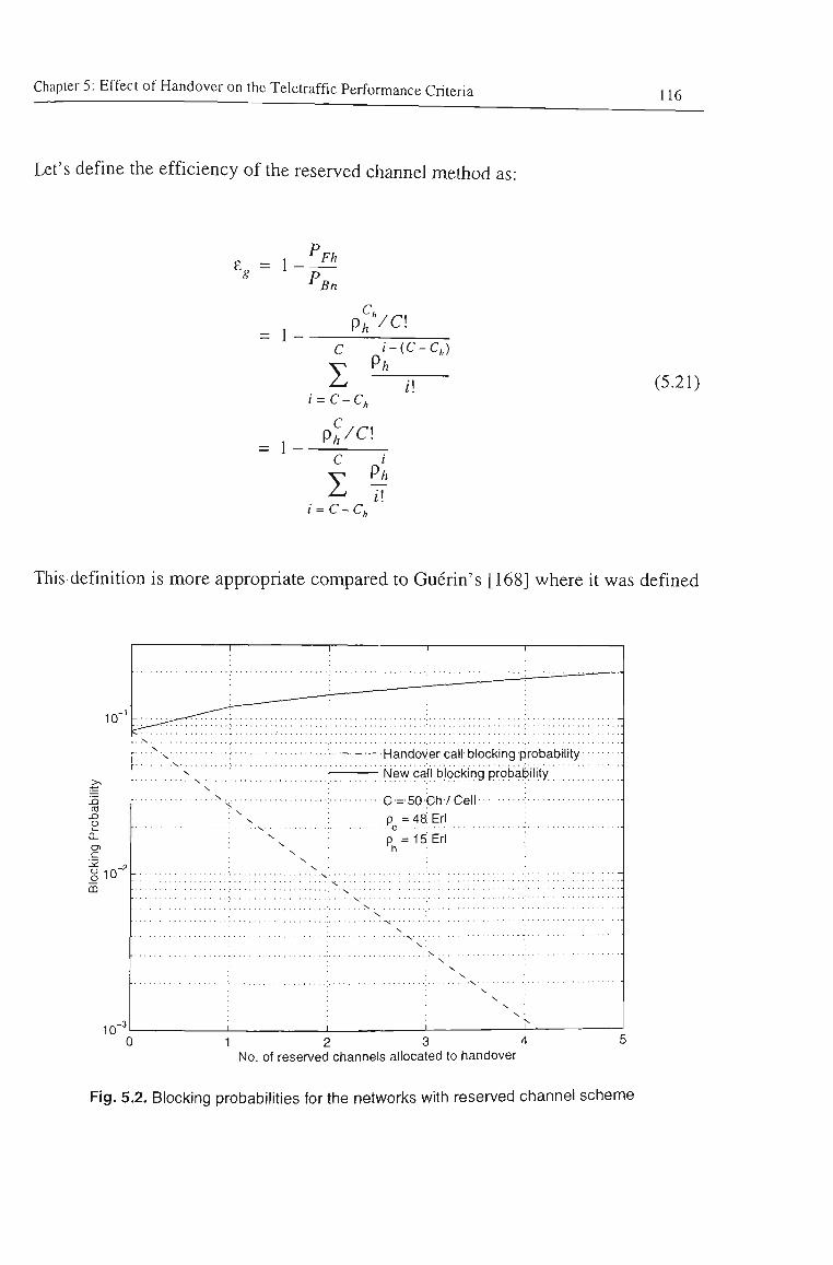
Chapter 5: Effect of Handover on the Teletraffic Performance Criteria 116
Let's define the efficiency of the reserved channel method as:
e„ = 1 Fh
Bn
= I p,VC!
C i-iC-C,)
= 1 -
i = C-C,
PI/C\ C i
^ i\ i = C-C.
ll (5.21)
This definition is more appropriate compared to Guerin's [168] where it was defined
10"
(0
o
c o o
CD
10"
.:— Handover call blocking probabtiity
Nevy call blocking probability
•C = 50Ch7Gell p =48;Erl
p =15Erl
10" 1 2 3 4
No. of reserved channels allocated to handover
Fig. 5.2. Blocking probabilities for the networks with reserved channel scheme
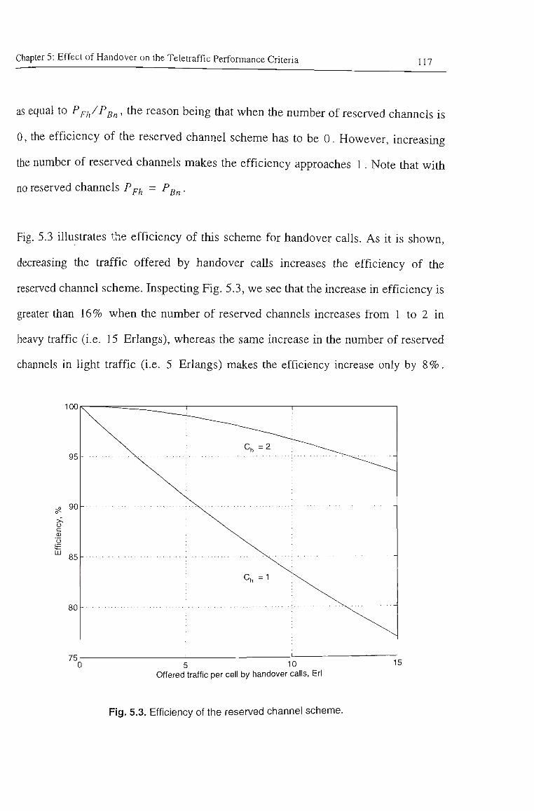
Chapter 5: Effect of Handover on the Teletraffic Performance Criteria 117
as equal to Pp^/Psn' the reason being that when the number of reserved channels is
0, the efficiency of the reserved channel scheme has to be 0. However, increasmg
the number of reserved channels makes the efficiency approaches 1. Note that with
no reserved channels P^^ = P, Bn-
Fig. 5.3 illustrates the efficiency of this scheme for handover calls. As it is shown,
decreasing the traffic offered by handover calls increases the efficiency of the
reserved channel scheme. Inspecting Fig. 5.3, we see that the increase in efficiency is
greater than 16% when the number of reserved channels increases from 1 to 2 in
heavy traffic (i.e. 15 Erlangs), whereas the same increase in the number of reserved
channels in light traffic (i.e. 5 Erlangs) makes the efficiency increase only by 8 %.
100
95
90
o
•9
lU 85
80
75
\ " ^——^^ '
c,
1
= 2 ^^^^--- . .^
= 1 ^ \
~~~~~~-~.<. , ;^
-
, 1
5 10 Offered traffic per cell by handover calls, ErI
15
Fig. 5.3. Efficiency of the reserved channel scheme.
Chapter 5: Effect of Handover on the Teletraffic Performance Criteria 11g
This reduction in efficiency at light traffic is not penalizing however, since at low traffic
blocking of handover calls is less likely. This shows that the reserved channel scheme is
most efficient when traffic is heavy and handover calls are most likely to be blocked.
5.4.2 Queueing prioritization schemes
Queueing prioritization schemes, with or without reserving channels for handover, is
another method of reducing the probability of forced termination at the expense of
increased new call blocking probability and a decrease in the ratio of
carried-to-offered traffic. The reason is that no new call is granted a channel before
the handover requests in the queue are served. Queueing prioritization schemes take
advantage of the fact that adjacent cells in a cellular network overlay each other.
Thus, there is an area where a call can be handled by either of the base stations. This
area is called the handover area. When a mobile station with an ongoing call enters a
handover area, it checks if there is a channel available on tiie new base station. If not,
handover request is buffered in a waiting queue, and the channel on the current base
station is used until a new channel is available. The fact that a successful handover
can take place anywhere in the handover area marks a certain amount of tolerance in
the delay in actual channel assignment after a handover request. The call eventually
is forced terminated if no channel is found in the new base station by the time tiie
mobile moves out of the handover area. Previous studies [101, 127, 165, 166]
indicate that the queueing schemes effectively reduce the forced termination
probability at the cost of slightly increasing the blocking probability of new call
attempts. However, the total number of unsuccessful calls of tiiese schemes are
roughly the same as those of nonprioritized schemes. Note that the performance of
Chapter 5: Effect of Handover on the Teletraffic Performance Criteria 119
the queueing schemes depend on the time that a mobile station stays in the handover
area. Two different methods are known for queueing prioritization schemes,
• First-In-First-Out scheme (FIFO)
• Measurement-Based Priority Scheme (MBPS)
hi the FIFO scheme [101], when a channel is released, the base station fkst checks if
the waiting queue is empty. If not the released channel is assigned to a handover call
in the queue based on the FIFO queueing pohcy. MBPS [165] is also sinular to tiie
FIFO scheme, except for the queueing policy. MBPS uses a non-preemptive dynamic
priority policy, for which priority calls are placed in the queue before all non-priority
calls, but never intermpt a call in progress. The priorities are defined by tiie power
level that the mobile station receives from tiie current base station. The network
monitors the power level of the queued handover calls dynamically, and assigns a
channel to the one with the weakest received signal.
In the general case, we consider queueing prioritization schemes in terms of reserving
channels for handovers. For this purpose three distinct cases can be identified, a) The
number of calls present in the system is less than 0-0^^, where all calls are served
without any distinction of type, b) The number of calls present in the system is equal or
more than C-Cf^ and less than C, where new calls are blocked and handover calls are
rved. c) The number of calls present in the system is more than C, and the new calls
blocked while the handover calls are queued. Basic queueing theory shows that the
probability of being in state i is ([148], Chapter 3 Section 1),
ser
are
Chapter 5: Effect of Handover on the Teletraffic Performance Criteria 120
P(0=
^^P(0) ll
c-Pe
C-Pe
-CI, i-Ph i\
-C, i-Ph
(C-
(C-
-c„)
- Q )
P(0)
c\c i-c
0<i<C-C,
C-Cf^<i<C
P(0) C<i
(5.22)
where, P(0) is the normalizing factor so that the state probabilities add up to 1, i.e..
P(0) 1 C-C,-li
2 7f-P C-C,
C-l i-iC-C,)
i = 0 1
i=C-C,
Ph +
C-C, C, Pe Ph
i\ ( C - l ) ! ( C - p , )
(5.23)
Therefore, the blocking probabihty of the new calls P^^ will be.
Ps, ^Prob{i>C-C^) = p,^^-C''
Ph
C-C, C, K Ph
i = C-C, il ( C - l ) ! ( C - p ; , )
P(0) (5.24)
It can be seen that the blocking probability of new calls when handover calls are
allowed to queue, is shghtiy greater than that of the case without queuing facility.
The fact that we have assumed infinite queueing capacity for handover calls imphes
that no handover call will be blocked, even if it undergoes a long waiting time.
Probability of a handover call being delayed P^^, can be obtained from tiie state
probabilities given in (5.22),
Chapter 5; Effect of Handover on the Teletraffic Perfonnance Criteria 121
C-C C
P « , = P ™ M . . C ) = ^ ^ P i L _ _ > i _ p ( 0 ) (5.25)
5.5 Simulation model
The' main aim of building a teletraffic simulation model is to obtain tiie appropriate
blocking probabilities, and for this purpose the length of time the network remains in
a certain state is not of any significance. Therefore, the proposed teletraffic
simulation model is based on the next-event time-advance approach which uses all
attributes of the current and next calls. These attributes include call duration, call
interarrival time, new call cell residence time and handover call cell residence time.
A very large population of mobile users is assumed in each cell, so that the mean call
arrival rate will be independent of the number of calls in progress. Mobiles are
assumed to be indistinguishable in the sense that the traffic originated per mobile is
the same. Call attempts associated with each mobile are taken to be one type only and
are assumed to arrive at the network according to a Poisson process. The call holding
times are assumed to be independent and identically distributed (iid ) random
variables, which follow the negative exponential distribution with a mean value of
I /\i^.&ec. The blocked-calls-cleared (BCC) queuing discipline has been selected.
New and handover call cell residence time distributions are taken to be generalized
gamma according to the results of mobility modelling in Chapter 4. It is also assumed
that a handover occurs from a cell to each of its six neighbouring cells with an equal
probability of 1/6. Further it is assumed that all base stations use omnidhrectional
Identically distributed means that different calls from different mobiles have the same probability distribution for the call holding time.
Chapter 5: Effect of Handover on the Teletraffic Performance Criteria 122
antennas.
5.5.1 Cellular IVIobile Coverage Area
A cellular mobile network usually covers a wide area, and is often difficult to
examine in its entirety by analytical means. In general, simulations are the only way
out of this situation. However, results from simulations are valid only if the cells
under consideration are sufficiently far away from the border of the cell stmcture. An
ideal cell stmcture would consist of an infinite number of cells and will have no
border which can affect the results. However, simulation of such a system is
impractical, since it needs virtually infinite memory and unacceptably long mnning
times. An altemative approach would be to find a finite network which
approximately represents the infinite network. One important issue arising from
changing an infinite network into an approximate finite one is the introduction of
edge effects in the finite network. Different types of approximate finite networks are
discussed in [169]. One way of accomplishing an approximately infinite cell pattem
is to wrap around the cellular layout with a limited number of cells [170]. By doing
this the cells are arranged in such a manner that they effectively constitute a
continuous toroidal surface. The problem with this kind of finite network is the
introduction of artificial dependencies between cells. If tiie chosen number of cells is
sufficiently large, tiiis effect is reduced. Fig. 5.4 shows the system which we have
used in the present simulation. The system comprises 49 cells witii a reuse cluster
size of 7 cells. Once tiie network is wrapped around, the cells with dashed lines will
become neighbours of the cells with sohd lines.
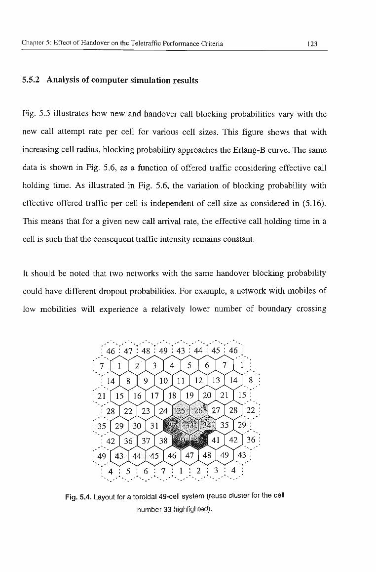
Chapter 5: Effect of Handover on the Teletraffic Performance Criteria 123
5.5.2 Analysis of computer simulation results
Fig. 5.5 illustrates how new and handover call blocking probabilities vary with tiie
new call attempt rate per cell for various cell sizes. This figure shows that with
increasing cell radius, blocking probability approaches the Erlang-B curve. The same
data is shown in Fig. 5.6, as a function of offered traffic considering effective call
holding time. As illustrated in Fig. 5.6, the variation of blocking probability with
effective offered traffic per cell is independent of cell size as considered in (5.16).
This means that for a given new call arrival rate, the effective call holding time in a
cell is such that the consequent traffic intensity remains constant.
It should be noted that two networks with the same handover blocking probabihty
could have different dropout probabilities. For example, a network with mobiles of
low mobilities will experience a relatively lower number of boundary crossing
Fig. 5.4. Layout for a toroidal 49-cell system (reuse cluster for the cell
number 33 highlighted).
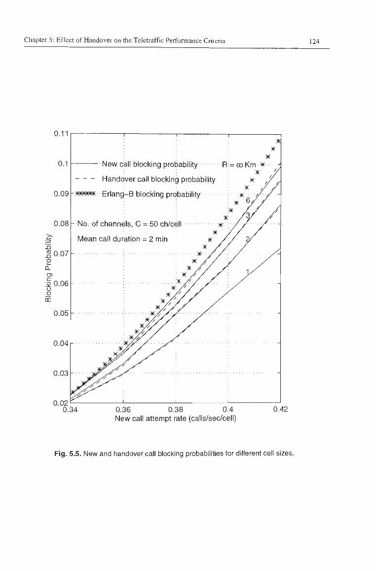
Chapter 5: Effect of Handover on the Teletraffic Performance Criteria 124
0.11
0.34 0.36 0.38 0.4 New call attempt rate (calls/sec/cell)
0.42
Fig. 5.5. New and handover call blocking probabilities for different cell sizes.
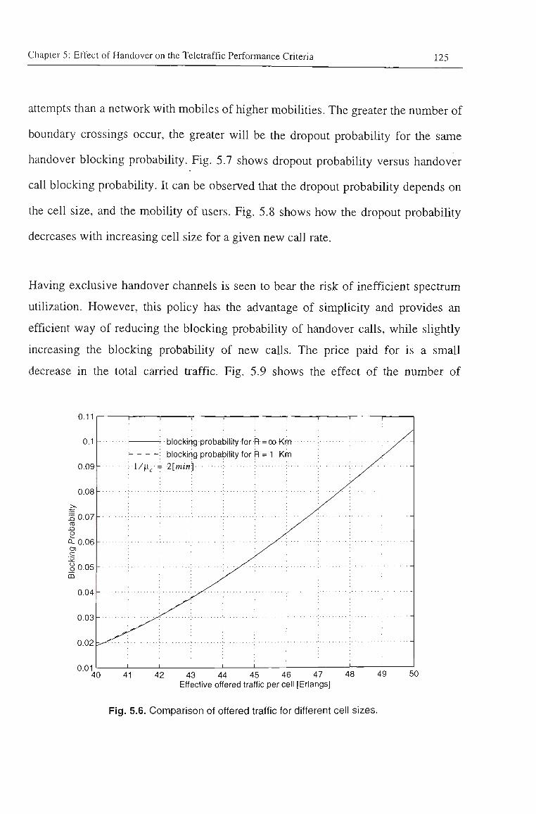
Chapter 5: Effect of Handover on the Teletraffic Performance Criteria 125
attempts than a network with mobiles of higher mobilities. The greater the number of
boundary crossings occur, the greater will be the dropout probabihty for tiie same
handover blocking probability. Fig. 5.7 shows dropout probability versus handover
call blocking probability. It can be observed that the dropout probabihty depends on
the cell size, and the mobility of users. Fig. 5.8 shows how the dropout probabihty
decreases with increasing cell size for a given new call rate.
Having exclusive handover channels is seen to bear the risk of inefficient spectmm
utilization. However, this policy has the advantage of simphcity and provides an
efficient way of reducing the blocking probability of handover calls, while shghtiy
increasing the blocking probability of new calls. The price paid for is a small
decrease in the total carried traffic. Fig. 5.9 shows the effect of the number of
0.11
0.1
0.09
0.08
B0.07 « O QlO.061-C
8 0.05 m
0.04
0.03-
0.02 >-
0.01
1
- ; i / ^ i c =
1
1 1 1 1
• blocking probability for R—00 Km blocking probability for R = 1 Km
1 1 1 1
!
1
40 41 42 43 44 45 46 47 48 Effective offered traffic per cell [Erlangs]
49 50
Fig. 5.6. Comparison of offered traffic for different cell sizes.
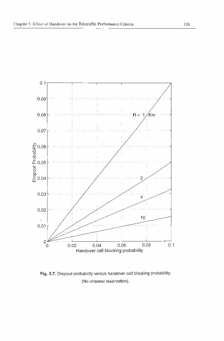
Chapter 5: Effect of Handover on the Teletraffic Performance Criteria 126
0.1
0.09
0.08-
0.07 -
i 0.06
o nIO.OS 3 o Q. O
0.04
0.03
0.02
0.01
0
1
^ ^ 1
. D . . . 1 . n — ly
o. . c.>
4
10
y
/Urr, -' T\m
0.02 0.04 0.06 0.08 Handover call blocking probability
0.1
Fig. 5.7. Dropout probability versus handover call blocking probability.
(No channel reservation).
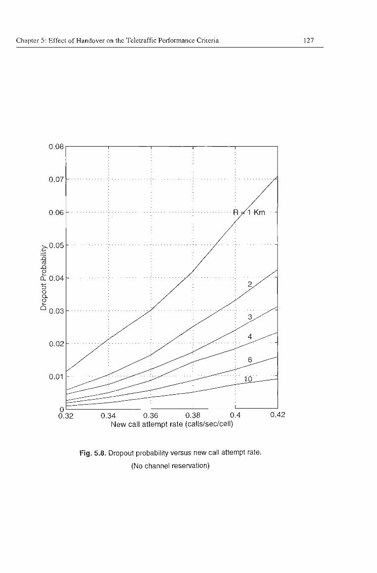
Chapter 5: Effect of Handover on the Teletraffic Performance Criteria 127
0.08
0.07
0.06-
.0.05
X2 CO
X2 O
Q- 0.04
o Q . O
0.03-
0.02-
0.01 -
0 0.32
1
; I
1
R V ^ Km -
2 X
3 / ^
6 ^ ^ ^
^_J0__-—
0.34 0.36 0.38 0.4 New call attempt rate (calls/sec/cell)
0.42
Fig. 5.8. Dropout probability versus new call attempt rate.
(No channel reservation)
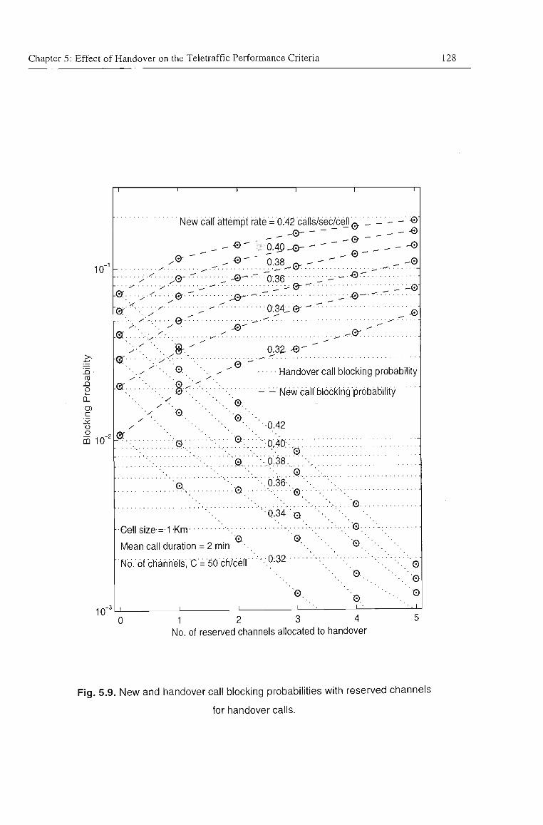
Chapter 5: Effect of Handover on the Teletraffic Performance Criteria 128
10"
CO X3 O
g A: o o m 10
10"
New call attempt rate = 0.42 calls/sec/cell'^''_ - - - ®
_ ^ - •© ' ? 0.40 - © - ' ' " ^ ^ - - - ® . © - " € > - ' n.38 ^ - - ' " _ - 0
^0-Of.
0: •0
.0:38^0:, '0-.3&
^ 0 -
'.^'.:Q.-r.
- .Q-_ _ ^ ^
•0-.34-&-^ •0
-0
Qr,...-..^.-.--0 ' .0:
0;
Gf.
0r
'0.
• y / • -
V O
q,3Z - 0 -
Handover call blocking probability
- -New cair blocking probability
.0-
0.:
0.
0.
"o •0.42
••o:4ff ©
0. 0.38. 0.
0, • 0 •,0.36-
0
0 Cell size— 1 Km
Mean call duration = 2 min
No. of chahnels,'C='50'ch/cefl
•Q.34-Q
• 0 .
•0.32 ••••
• 0 .
. • . . . . . •©.
0
0. I
0.
0 I -
1 2 3 4 No. of reserved channels allocated to handover
Fig. 5.9. W&N and handover call blocking probabilities with reserved channels
for handover calls.
Chapter 5: Effect of Handover on the Teletraffic Performance Criteria 129
reserved channels allocated to handover on the probability of handover attempt
failure and the new call blocking probability. As can be seen, the rate at which the
blocking probability of handover calls decrease with increasing number of reserved
channels is much bigger than the rate at which the new call blocking probability
increases.
The use of reserved channels requires careful determination of the optimum number
of reserved channels. This in turn requires the knowledge of the traffic pattem of the
area, and an estimation of the channel occupancy time distributions. Reserving
channels for handover means less channels are left for new calls so that the total
carried traffic is reduced. This disadvantage can be minimised by carefully selecting
the number of reserved channels. Also, it can be overcome to a certain extent by
allowing queueing of new call attempts, which are considerably less sensitive to
delays than handovers.
As it was mentioned earlier, using channel reservation priority scheme reduces
dropout probabihty. Fig. 5.10 shows the effect of the number of reserved channels on
the dropout probability for different offered traffic. It can be seen that tiie dropout
probability decreases with the increasing number of reserved channels. This
reduction is paid for by an increase in the new call blocking probability. The possible
compromise between the new call blocking probabihty and the dropout probability
can be established by allocating a tiu-eshold level on the dropout probabihty. Fig.
5.11 indicates tiie necessary number of channels exclusively dedicated to handover in
order to obtain a certain limit on dropout probability.
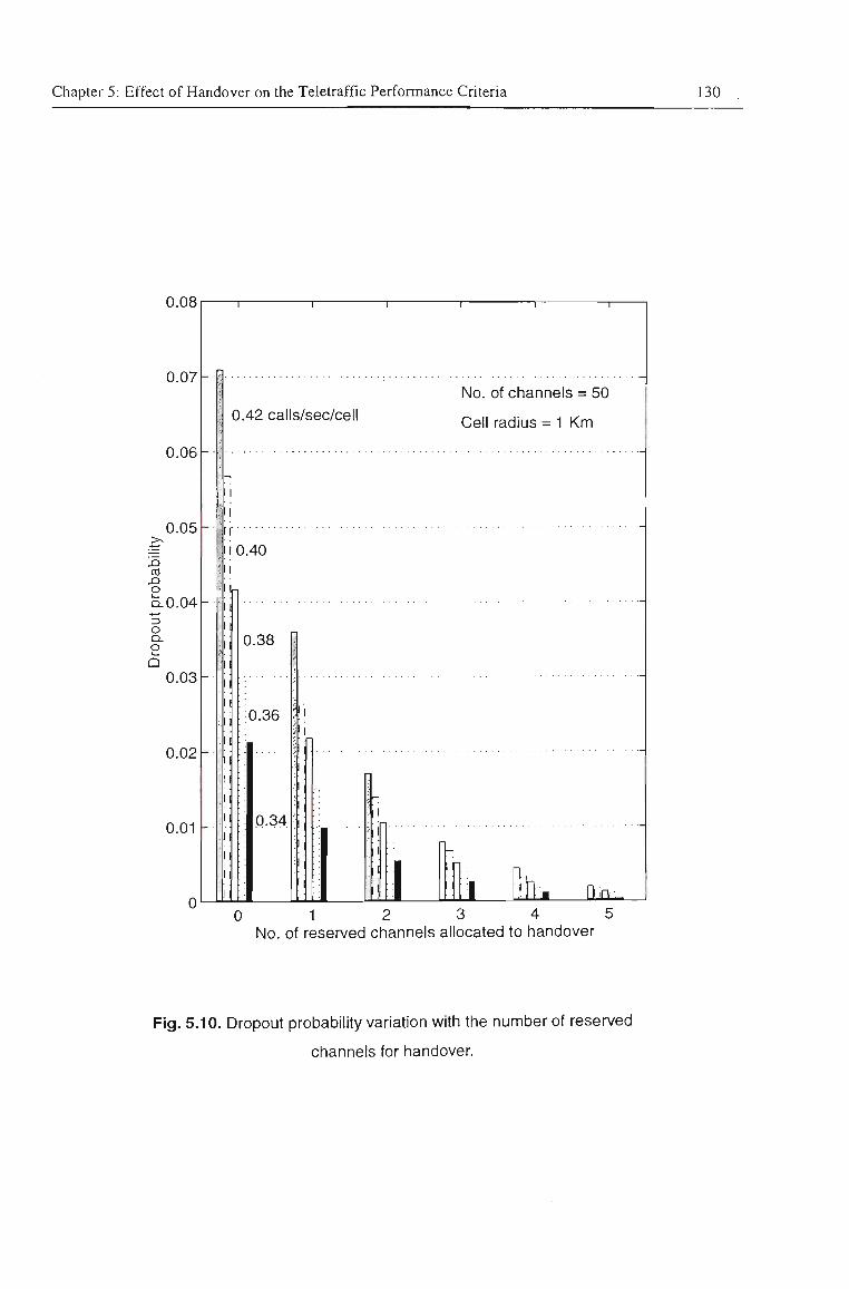
Chapter 5: Effect of Handover on the Teletraffic Performance Criteria 130
0.08
0.07
0.06
0.05-
X3
^0.04
o Q. O
0.03
0.02
0.01
0"-^
0.42 calls/sec/cell
0.40
0.38
0.36
0.34
I
No. of channels = 50
Cell radius = 1 Km
I I H. Jlil. 0 1 2 3 4 5
No. of reserved channels allocated to handover
Fig. 5.10. Dropout probability variation with the number of reserved
channels for handover.
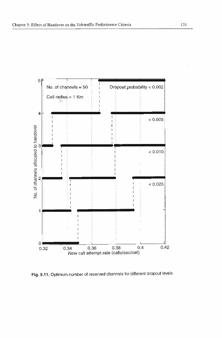
Chapter 5: Effect of Handover on the Teletraffic Performance Criteria 131
> O •a c: CO
sz 2 3 O
CO o
To
CD
§2 x: o "o 6
X !
; No. of channels = 50
• Cell radius = 1 Km
^^^
^^ 1
1 Dropout probability < 0.002:
^^^^
< 0.005.:
< 0.010
< 0.025:
1 T
0.32 0.34 0.36 0.38 0.4 New call attempt rate (calls/sec/cell)
0.42
Fig. 5.11. Optimum number of reserved channels for different dropout levels
Chapter 5: Effect of Handover on the Teletraffic Performance Criteria 132
5.6 Conclusions
In this Chapter different radio resource allocation schemes were explained, teletraffic
performance criteria were defined, and an analytical model for teletraffic analysis
was presented. Also, some traffic policies that give a higher level of protection to
handover calls were analysed, ai:d their effects on the overall traffic perfonnance
were described. Based on the results obtained in Chapter 4, a teletraffic model that
takes the user mobility into account was presented and was substantiated using a
computer simulation based on the next-event time-advance approach. Furthermore,
the influence of cell size on new and handover call blocking probabilities was
examined. The effect of handover channel reservation policy on call dropout and
handover failure probabilities was also examined to determine the optimum number
of reserved channels required for handover.
It was found that blocking probabilities of the new and handover calls are the same when
there are no reserved channels for handover calls. These probabilities become different
with the allocation of some channels for handover calls. The variation of blocking
probabilities of new and handover calls are such that any decrease in the blocking
probability of the handover calls is much bigger than the corresponding increase in
blocking probability of the new calls. This fact makes the reserved channel scheme
attractive. An efficiency factor was defined to show the effectiveness of this scheme. It
was shown that the reserved channel method is most efficient when the traffic is heavy
and handover calls are most likely to be blocked.
It was also shown that with increasing cell radius, blocking probability approaches the
Erlang-B curve. However, the blocking probability variation with respect to the effective
Chapter 5: Effect of Handover on the Teletraffic Performance Criteria 133
offered traffic per cell is independent of the cell size and follows Erlang-B formula. This
means that for a given new call arrival rate, the effective call holding time in a cell is
such that the consequent traffic intensity remains constant. It was also found that the
dropout probability decreases with increasing number of reserved channels. This
reduction is paid for by an increase in the new call blocking probability. The
compromise between the new call blocking probability and the dropout probability is
established by allocating a threshold level on the dropout probability.
Chapter 6
Mobile Radio Channel Modelling
for Handover Analysis
In cellular systems, a knowledge of received signal behaviour is essential to analyse
the handover, power control, and dynamic channel allocation. In fact, signal strength
measurement represents the most important parameter for any reliable handover.
Consequently, a thorough investigation and characterization of signal strength is
required. The propagation of radio waves is always associated with the
unpredictibility of the medium which generally varies in space and time. In cellular
mobile radio communication systems, the mobile nature of the users and small
clearance of the mobile antenna from the ground impose additional constraints on the
predictability of the received signal.
Chapter 6: Mobile Radio Channel Modelling for Handover Analysis 135
The mobile radio channel environment belongs to the class of non stationary random
fields, where the received signal is affected by different factors such as base and
mobile station characteristics as well as natural terrain and man-made stmctures.
In planning service areas for mobile radio communication systems, calculation of the
path loss as well as precise estimation of the signal variabihty is absolutely
necessary. The complex nature of the radio propagation in the real world makes exact
analytical computation impossible. Whilst these data can be obtained from field
surveys, the problem with this approach is that it is time consuming and expensive.
Therefore, computer simulations are widely used. The models employed for these
simulations are mainly a mixture of both theoretical and empirical relations as well as
added stochastic processes. In generic system studies, a suitable model for variabihty
of propagation phenomena can be derived by applying statistical communication
theories, without considering any specific terrain data.
6.1 Radio Signal Components
A mobile radio channel is usually characterized by the superposition of three
different, mutually independent, multiphcative, and approximately separable
components with small-, medium-, and large-scale propagation effects. The
small-scale quasi-stationary variations, mostly referred to as multipath fading, are
fairly rapid in space. Medium-scale effect, mostly referred to as shadowing, is
influenced by the spatial movements of the order of tens of wavelengths and creates
random variations in tiie average power of tiie received signal which typically
follows a lognormal distribution. In the large-scale effect, spatial movements of tiie
Chapter 6: Mobile Radio Channel Modelling for Handover Analysis 136
order of hundreds of meters make the median average power level vary in power-law
fashion with path length. Large-scale variation is mostly referred to as path loss.
Shadowing creates local variations (narrow area median), while path loss creates
long range variations (wide area median).
The instantaneous radio signal received at tiie mobile can be expressed as r{t)e'^ ,
where (p(f) is a random variable, denoting phase angle of the received signal. In this
work, we are interested in the received signal envelope r{t), which can be described
as the product of a slow varying signal s^{t) (shadow fading component), and of a
rapid variation factor r^{t) (multipath fading component) 1171]. Therefore,
r{t) = s^{t)-r^{t) (6.1)
The received signal envelope r{t) at time t is an average over the modulation (e.g.,
over the data symbols in digital cellular), so that it can be studied without regard to
the particulars of the modulation. Equation (6.1) can also be expressed in tiie spatial
domain, since the time fluctuations result from subscriber movement through the
spatial fluctuations of signal power density. Therefore,
r{x) = s^{x) • r,(x) (6.2)
6.1.1 Multipath fading component
Local scatterers around the mobile produce several time-delayed and attenuated
versions of the original transmitted signal. Consequentiy, the received signal
Chapter 6: Mobile Radio Channel Modelling for Handover Analysis 137
comprises a summation of several signals which can add together either
constmctively or destmctively. The resultant field strength in such an environment
follows a spatially-fluctuating standing-wave pattem with minimum and maximum
values a quarter-wavelength apart. Movement of a mobile station through such a
space-selective fading field makes the receiver sense a time-selective fading signal.
The rat(?3 of fluctuation depends on the velocity of the mobile and the result is a
received signal level which experiences very large and fast variations. The
assumption that different scattered wave components are mutually uncorrelated with
random phase leads to the conclusion that the local statistics of the received signal
envelope follows a Rayleigh distribution. The signal envelope r has a Rayleigh
distribution, if measured over distances of a few tenths of a wavelengtii, where the
average signal is a quasi-stationary process (approximately constant) over small
areas. Therefore, the probability density function of the received signal envelope r
relative to the local mean s^ = <r), can be represented by 184, 172],
2
-nr
f{r\sj = ^ 2 / ^ " ' U{r) (6.3)
2 ^ .
where U{r) is the unit step function.
In a microcellular environment, radio propagation often includes a line-of sight
(LOS) path which makes tiie short-term statistics of the received faded signal
envelope to include a constant term. In tiiis case, examination of statistical
distiibution of the received signal envelope relative to tiie local mean shows tiiat it
Chapter 6: Mobile Radio Channel Modelling for Handover Analysis 138
most likely conforms to Rician distribution and suffers significantly less multipath
fading, compared to the case of Rayleigh faded channel. Therefore, the probabihty
density function of the received signal envelope relative to the local mean can be
represented by:
- ^ Y t A
f(r\So) = j e lo 2s o
o 2 U{r) (6.4)
where ^ is the positive offset value from the Rayleigh distribution (amplitude of
direct wave), and I^{ ) is the modified Bessel function of the first kind zero order.
6.1.2 Shadow fading component
As the vehicle moves, changes in the obstacles along tiie propagation path lead to the
gradual changes in local mean level s^. Analysis of mobile radio propagation
measurement results from different surveys has shown tiiat the local mean of tiie
signal envelope r is adequately described by a lognormal distribution. That is, tiie
local mean s = 201og ^o in dB is a Gaussian random variable, with a probability 10
density function given by:
-is-\i)'
f(s) = -j^e '""^ (6-5)
where a . is the standard deviation of the local mean in dB due to the shadowing of
Chapter 6; Mobile Radio Channel Modelling for Handover Analysis 139
the signal {location variability), and p = (s) is the average of the received signal
local mean level {area average) in dB. Area average reflects the median logarithmic
attenuation and can be determined by the path loss. The value of a^ has been
experimentally found to lie between 3 ~ l2dB [173, 174]. This broad range can be
attributed to variations between experiments in the presence or absence of the LOS
,.^ component (LOS component increases o^), the height of the antennas used (lower,
antennas decrease a^), the spatial averaging window length (longer windows
decrease a^), or the type of the terrain. Mogensen et al. [175] have shown that a^ is
relatively independent of frequency. Berg et al. [176] and Goldsmith et al. [173] have
proposed a value of 4dB in urban microcell areas, whereas for suburban areas
containing macrocell areas the value is more likely to be 8dB [177].
6.1.3 Path loss component
In the mobile radio environment, due to tiie fact that tiie mobile antenna height is
close to the ground, the signal received from the base station is affected by tiiree main
sources of loss, namely, free space loss, ground wave loss and diffraction loss. The
path attenuation depends on many variables, some of which can be controlled (e.g.,
frequency, antenna height); some can be measured (e.g., distance); and some can
neither be controlled nor be measured deterministically (e.g., climate, topography of
the environments, terrain). Considering all these factors, it is apparent that the path
loss prediction of mobile radio signals is a formidable task. Although there is no easy
analytical solution to tiie problem, it is possible to create a propagation prediction
model to estimate the median patii loss. These models vary in complexity, accuracy,
and capability. Among different metiiods, Hata's empirical formula based on
Chapter 6: Mobile Radio Channel Modelling for Handover Analysis 140
Okumura's measurements is the most widely used relation that predicts the median
propagation path loss in macrocells [178]. The median path loss, L , in decibels
between two isotropic base and mobile antennas, with a separation distance denoted
by d in kilometre is formulated as:
L^ = A -I- lOylog J (6.6)
where y is the slope factor and depends on the base station effective antenna height
/i^, and is weakly affected by the carrier frequency. A good approximation yields
Y = 4.49-0.655 log/i^. The value of A for different frequency and envhonment
settings such as urban area, suburban area, open area can be obtained through Hata
and Okumura recommendations [178]. Therefore, in case a transmitter emits a signal
with the power of Ptxi<^B], the received signal level Prxi^B] due to tiie patii loss
will be:
Prx = Ptx-h = ^^-^2^^^'^ (6.7)
where, K^ = P,^-A and i^2 = lOy. Hata's formula does not consider propagation
from low base station antenna heights (less than 30m) or over the short distance (less
than I Km). Therefore, in a microcellular environment, where ceU radius is usually
below I Km, and base station antenna height is lowered down the surrounding
buildings at tiie street-lamp elevation, Hata's formula is not valid.
One of the main distinctions between tiie propagation characteristics of the
microcells and macrocells is tiie existence of a LOS wave. The presence of a LOS
Chapter 6: Mobile Radio Channel Modelling for Handover Analysis 141
path in the microcell environment implies that, in a region near the base station, the
environmental features are unlikely to have a prominent influence on the propagation
conditions, and the path loss exponent will be very close to that of free space
propagation. When the link distance grows beyond a limit, namely a breakpoint
distance, environmental factors dominate and path loss exponent increases, which
leads «o extra attenuation. The exact position of the breakpoint has been reported
anywhere from 150-300m by a number of authors [54, 179]. Xia et al. [180]
demonstrate that the breakpoint is the point where the Fresnel zone between the two
antennas touches the ground assuming a flat earth. Therefore, the propagation path
loss in microcells can be characterized by two straight lines with different slopes.
Another issue which commonly exist in microcells of Manhattan type is the street
corner effect. Tuming around a street comer causes a dramatic decrease in the
received signal strengtii of the mobile station, due to the blockage of LOS
component. In order to minimise the error occurring from this in tiie microcellular
environment propagation model, tiie propagation phenomena are broken down to two
categories as line-of-sight (LOS) and non-line-of-sight (NLOS) emissions.
The received signal strength p^^, at a distance of x from a transmitter witii the output
power of p^, and the wavelengtii of X can be predicted by [176]:
P' ("^ \ - - (6.8) P'-' ~ L{x) 'W' • ^' • ^
where g, and g^ are the transmitter and the receiver antenna gains relative to the
Chapter 6: Mobile Radio Channel Modelling for Handover Analysis 142
isotropic counterparts. L{x) is given by:
w=i r-ji4 r""" ' («) ^ Q / A/ V-^i
where ^ is a form factor which determines the smoothness of the variation of the
path loss at the transition region around the breakpomt x^. XQ, m are two parameters
whose values along witii the values of tiie parameters q, x^ are chosen as suggested
in [176]. Assuming that a fictitious transmitter is located at tiie street crossing, at a
distance x^ from the base station, a similar loss relation in a side street for NLOS
case can be found. In this case (6.9) can be stated as tiie following:
Again tiie values of parameters y^, y^, q, n are chosen as suggested hi [176]. Fig. 6.1
illustrates definition of x, x^, y, y^. The total loss along a NLOS stieet is determined
by:
L(x,,y) = L{xJ-L{y) (6.11)
The received signal power could be obtained by substittiting L{x^, y) in place of
L(x) in (6.8).
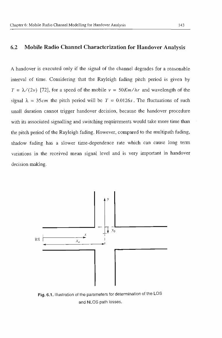
Chapter 6: Mobile Radio Channel Modelling for Handover Analysis 143
6.2 Mobile Radio Channel Characterization for Handover Analysis
A handover is executed only if the signal of the channel degrades for a reasonable
interval of time. Considering that the Rayleigh fading pitch period is given by
T - X/{2v) [72], for a speed of the mobile v = 50Km/hr and wavelength of the
signal X = 35cm the pitch period will be T = 0.01265'. The fluctuations of such
small duration cannot trigger handover decision, because the handover procedure
with its associated signalhng and switching requirements would take more time than
the pitch period of the Rayleigh fading. However, compared to the multipath fading,
shadow fading has a slower time-dependence rate which can cause long term
variations in the received mean signal level and is very important in handover
decision making.
BS
iy
X 1 yo
Fig. 6.1. Illustration of the parameters for determination of the LOS
and NLOS path losses.
Chapter 6: Mobile Radio Channel Modelling for Handover Analysis 144
A proper selection of the size of spatial window is needed to effectively smooth out
the Rayleigh fading variation. Lee [47] and Austin et. al [85], have investigated
guidelines for the minimum distance averaging interval needed to eliminate fading in
macrocells and microcells, respectively. Work carried out by Lee [47] suggests a
length of 40 A, as a suitable distance in the case of macrocells. If the length is shorter
than 40A-, the average output would still retain a weaker portion of Rayleigh fading.
If the length is greater than 40A-, the excessive length of averaging also smooths out
the local mean information. In practice, a spatial window in the range 20A. to 40A, is
acceptable.
Examination of data taken from microcells shows that Rayleigh fading variation is
less severe but the local mean could suffer quite large variations over short distances.
In microcells, moreover, large window length may conceal the steep decrease of the
signal strength when the mobile turns around a street-comer. Green [181] suggests a
spatial window size of 5X as an appropriate averaging length for microcells.
Velocity adaptive sampling is assumed to maintain spatial window lengths at a
constant value. The received signal strength averaged over tiie window ^(0 is a
stochastic process where the first order statistics of that, at any instant of time or
equivalently at any distance, can be modelled as a correlated lognormally distributed
variable s with an average value of p and a standard deviation of a^. Since signal
variation is a limited amount, s can be considered as a tmncated normal distribution
bounded within the range ±3a^. The mean received signal level can be predicted
using a model which consists of a median path loss |i and a log-normal variation of
the local mean due to shadowing, S. Therefore,
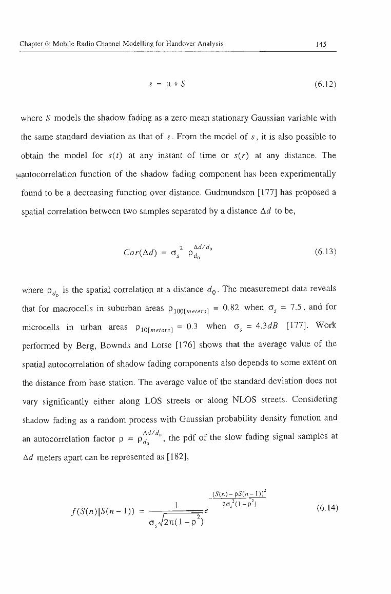
Chapter 6: Mobile Radio Channel Modelling for Handover Analysis 145
s = ]1 + S (6.12)
where S models the shadow fading as a zero mean stationary Gaussian variable with
the same standard deviation as that of s. From the model of 5, it is also possible to
obtain the model for s{t) at any instant of time or s{r) at any distance. The
^autocorrelation function of the shadow fading component has been experimentally
found to be a decreasing function over distance. Gudmundson [177] has proposed a
spatial correlation between two samples separated by a distance Ad to be.
CoriAd) = a / p^''" (^.13)
where p^ is the spatial correlation at a distance dQ. The measurement data reveals
that for macrocells in suburban areas pioo[meters] = ^-^^ ^^^" ^s = '^•^' ^^^ ^^^
microcells in urban areas PiQ[^eters] = ^-^ ^^^^ ^s = 4-3^5 [177]. Work
performed by Berg, Bownds and Lotse [176] shows tiiat tiie average value of tiie
spatial autocorrelation of shadow fading components also depends to some extent on
the distance from base station. The average value of tiie standard deviation does not
vary significantly eitiier along LOS streets or along NLOS streets. Considering
shadow fading as a random process with Gaussian probability density function and
an autocorrelation factor p = p^'^/'^", the pdf of the slow fading signal samples at
Ad meters apart can be represented as [182],
( 5 ( n ) - p 5 ( n - l ) ) '
1 2 a / ( l - p ^ ) (-6 1/1^ f{S{n)\S{n-l)) = ——==e (6-14)
oJ2n{l-p )
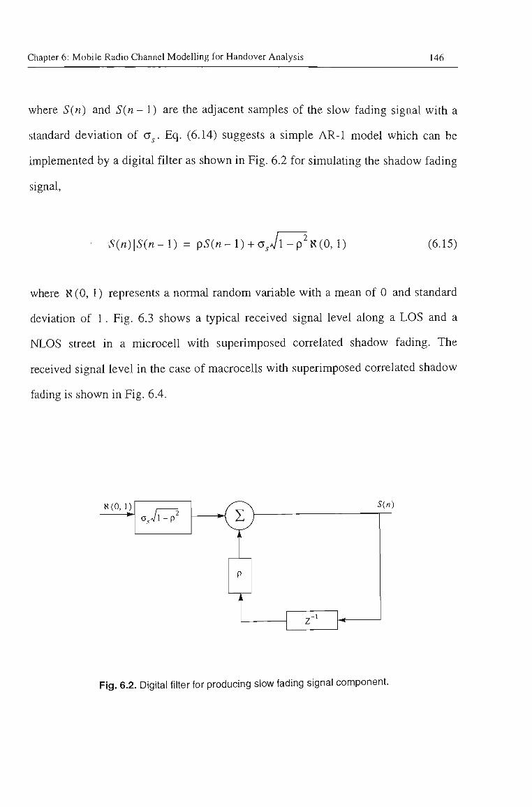
Chapter 6: Mobile Radio Channel Modelling for Handover Analysis 146
where S{n) and S{n - 1) are the adjacent samples of the slow fading signal with a
standard deviation of a^. Eq. (6.14) suggests a simple AR-1 model which can be
implemented by a digital filter as shown in Fig. 6.2 for simulating the shadow fading
signal.
S{n)\S{n-l) = pS{n-l) + aJl -P X(0, 1) (6.15)
where K (0, 1) represents a normal random variable with a mean of 0 and standard
deviation of 1. Fig. 6.3 shows a typical received signal level along a LOS and a
NLOS street in a microcell with superimposed correlated shadow fading. The
received signal level in the case of macrocells with superimposed correlated shadow
fading is shown in Fig. 6.4.
N(0, 1) ojl - p ^ /
^\
^ - " ^
1
\ )
k
P
i I
Z-'
S{n
Fig. 6.2. Digital filter for producing slow fading signal component.
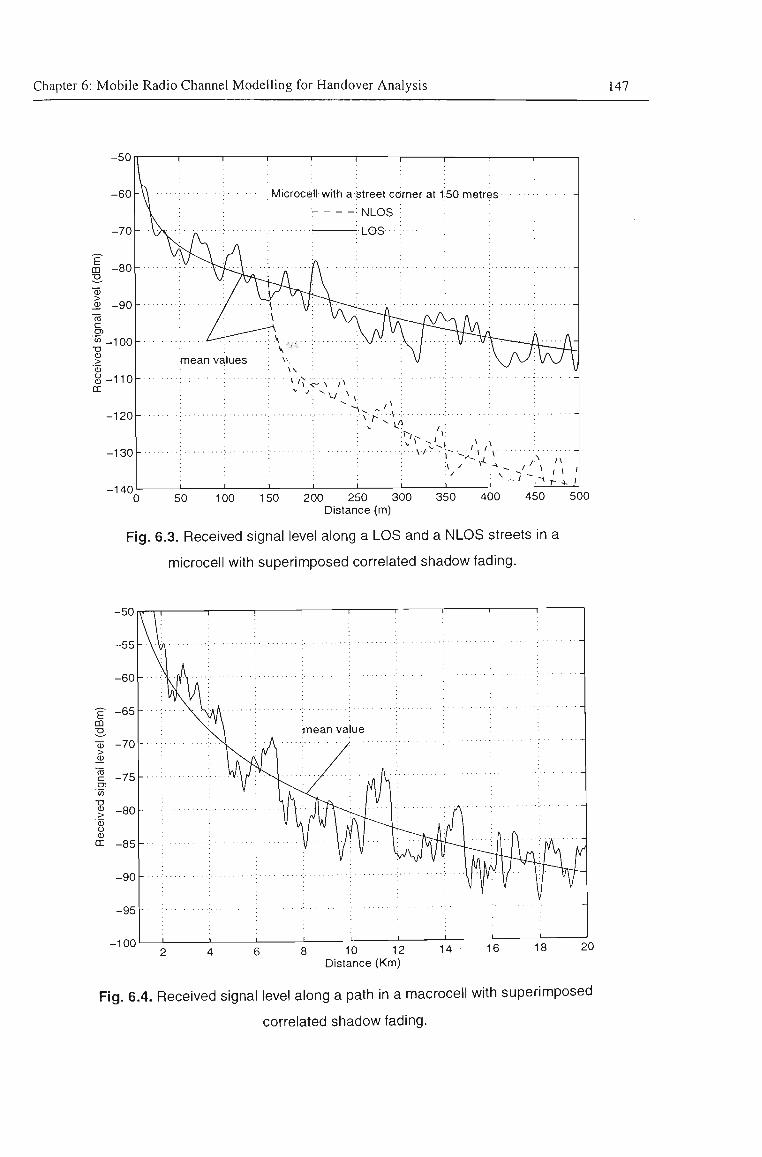
Chapter 6: Mobile Radio Channel Modelling for Handover Analysis 147
E m
•53 > 0) ^ - 9 0
c
" - 1 0 0 T3
> O o cc
-130
Microcell witti a street ccirner at-150 metres
: ; NLOS ;
-[JOS •:
0 50 100 150 200 250 300 350 400 450 500 Distance (m)
Fig. 6.3. Received signal level along a LOS and a NLOS streets in a
microcell with superimposed correlated shadow fading.
-50
-55
- 6 0
-§- - 6 5 CD
o - 7 0 > CD
S -75 '(/> -a I -80
•53 o
CC - 8 5
- 9 0
-95
-100
v \
. . . .
1 ! 1 I ! 1 ! 1
>v \ rnean value
i , 1 _ i 1 1 ' '
8 10 12 Distance (Km)
14 16 18 20
Fig. 6.4. Received signal level along a path in a macrocell with superimposed
correlated shadow fading.
Chapter 6: Mobile Radio Channel Modelling for Handover Analysis 148
6.3 Conclusions
The contributions of three different components of a mobile radio signal are
considered, and a propagation model suitable for micro- and macro-cells has been
presented. Emphasis is made on the effect of shadow fading (the medium-scale
propagation component), which is most important in handover decision making in
cellular networks. It has been shown that a simple AR-1 model can be implemented
by a digital filter for simulating the shadow fading signal taking correlation between
adjacent samples into account.
Chapter 7
Optimum Hysteresis Levels Signal
Averaging Time and Handover
Delay
Performance of inter-cell handover algorithm is critical to the overall performance of
a cellular mobile communication system. When a mobile station crosses a cell
boundary between two base stations, handover is required to switch the radio link of
the mobile station from the departing base station to the approaching base station in
order to maintain the connection. The cmcial part of handover is to decide exactly at
which point a handover should take place. In analog systems this is solely determined
by the received signal strength profile of the mobile station. In digital cellular
systems other criteria have also been suggested. In GSM, quality of the received
signal (as reflected by the bit error rate), and the distance between mobile and the
Chapter 7: Optimum Hysteresis Level, Signal Averaging Time and Handover Delay 150
base station (as measured by the timing advance), have been recommended.
However, careful examination of the handover algorithms chosen for implementation
by several equipment manufacturers of GSM system indicates that these otiier
criteria serve mainly in recognition of abnormal operating conditions (known as
alarm conditions) rather than in providing a primary input to the handover decision
making process. Thus, even in digital cellular systems, it is tiie mobile received
signal strength that provides the vital information required for handover decision
making.
As is discussed in Chapter 6, in the envhonments in which the cellular mobile
systems operate, the received signal strength of a mobile station along its path is
hardly a monotonic function even when the mobile moves in a straight line directly
across cell boundaries separating the two base stations. The irregularities of terrain,
the built up stmctures in urban areas and the like cause fluctuations in the received
signal strength, making it difficult to determine the exact position at which the
handover should occur.
The mobile received signal can be considered as consisting of three components,
namely, the path loss component, the slow fading shadow component and the fast
fading multipath component. The path loss component is determined primarily by the
distance between the base station and the mobile station. In the absence of fading,
this causes the signal strength to decrease gradually with distance. It is the path loss
component that provides the best guide in the determination of the appropriate point
of handover. However this is often obscured by the presence of the fading
components of the signal causing confusion in making an appropriate handover
Chapter 7: Optimum Hysteresis Level, Signal Averaging Time and Handover Delay 151
decision. As a result the radio link may be switched back and forth between
neighbouring base stations jeopardizing the call quality and increasing the chance of
a lost call. This phenomenon, i.e. repeated handovers between two base stations, is
called the ping-pong effect. An improperly designed handover algorithm results in an
unacceptably high level of ping-ponging which could give rise to high signalling costs in
addifaion to increasing the probability of forced termination of calls.
An optimal handover algorithm should reflect the optimal tradeoff between the caU
quality (i.e., higher signal to noise ratio) and the signalling cost. If the handovers
could be accomplished without any signalling cost, the best algorithm will be the one
which connects the mobile station to a base station with the highest signal strength at
each instant. However, in the presence of non-zero signalling costs, a better handover
algorithm is one which also minimises the number of unnecessary handovers. The
handover algorithm proposed in GSM provides, among other tilings, a handover
margin (hysteresis) to be incorporated in tiie process as a means of preventing
unnecessary handovers. However, a suitable value for tiiis parameter has to be
determined in conjunction with the other parameters involved in the processing of the
mobile received signal.
For instance, a short signal averaging time may resuh in an increase in unnecessary
handovers, while a long averaging time may resuU in a failure to detect a necessary
handover. Introduction of a hysteresis level ensures tiiat necessary handovers occur,
while the unnecessary handovers are reduced if not eliminated totally. However,
application of tiie hysteresis level leads to a delay in the handover decision and has to
be kept as smati as possible. Therefore, care should be taken in choosing tiie signal
Chapter 7: Optimum Hysteresis Level, Signal Averaging Time and Handover Delay 152
averaging period and the hysteresis level to achieve the optimum trade-off between
the number of unnecessary handovers and the delay in handover.
7.1 Handover Initiation Parameters
1^' The two significant design factors influencing tiie performance of tiie handover
initiation based on the received signal strength include: (a) control mechanisms to
limit the numbers of unnecessary handovers, such as tiie hysteresis level, the signal
threshold level, tiie lengtii and shape of averagmg window and, (b) parameters
effecting the time of a handover decision such as the averaging period, sample
interval size and the detection time.
Both experimental and analytical models for handover algorithms have been reported
in the literature. Gudmundson [59] has proposed a class of linear handover
algorithms, in which the decision is based on the linear characteristics of the signal.
He suggests that an optimal handover decision is possible when the future value of
the signal is known exactly. Chia and Warburton [58] have presented experimental
results for handover using signal strength averaging. They examined the probability
of handover and the effects of hysteresis. Vijayan and Holtzman [57, 183] have
studied the dynamic behaviour of handover algorithms based on field strength
measurements in a fading environment. The analysis is carried out in terms of level
crossings of a stochastic process which is the difference between two processes, each
representing the signal strength from a base station. At first, the level crossing
process was assumed to be stationary; later work [62] included the nonstationary
case. Zhang and Holtzman [69] have extended the case of relative strengths to the
Chapter 7: Optimum Hysteresis Level, Signal Averaging Time and Handover Delay 153
case of combined absolute and relative strengths. The reported results indicate the
possible tradeoff between delay and the expected number of unnecessary handovers
when the averaging interval is fixed. They show that as either the hysteresis margin is
raised or the signal threshold level lowered, the mean number of unnecessary
handovers decreases and the expected delay increases. When the hysteresis level is
small fis&:the considered parameters, the threshold has a greater influence on the
expected number of unnecessary handovers and crossover points. Murase, Symington
and Green [61] also have looked into the effect of signal averaging time on the
hysteresis level and handover performance. Ruggieri et. al [184] have extended the
model in [57] to account for the effects of the mobile's movement direction, the
effects of the cross-correlation of shadow fading and the presence of more than two
base stations.
Corazza et al. [185] have evaluated the trade-off between delay and number of
unnecessary handovers based on a simulation study. Their work have focused on the
shape of the averaging window, and have considered both rectangular windows and
exponential windows witii various weights. Results show that long averagmg periods
reduce the number of unnecessary handovers but increase the delay. Kwon et al.
[186] have investigated handover algorithms for various hysteresis levels and overlap
conditions. Bernhardt [187] has studied the performance of handover in a
frequency-reuse time-division multiplexed system via a computer simulation. He has
shown that handover based on tiie comparison of time-averaged relative power of
different channels, combined witii hysteresis, can be the nucleus of an effective
trigger mechanism.
Chapter 7: Optimum Hysteresis Level, Signal Averaging Time and Handover Delay 154
Dassanayake [56] has investigated the effects of averaging the measurement samples
of signal strength and the hysteresis setting of the handover algorithms on the
elimination of unnecessary handover requests. A computer simulation based on a
four cell model consisting of a serving cell, a target cell and two neighbouring cells
has been used. Senadji et. al [188] have studied optimization of two confhcting
criteria, the number of unnecessary handovers and the numbiii of lost calls due to
dropout. Their study was based on the Bayes criterion which is commonly used in
detection and estimation techniques. However, this algoritiim requires a real-time
computation of a dynamic threshold. This computation leads to an increase in
decision time which is an undesirable effect.
Senarath et. al [189] have shown that under realistic prediction schemes, depending
on the mobile environment (mobile speed and direction, shadowing correlation and
cell layout), an improvement in the call dropout performance can be obtained tiirough
hysteresis schemes in addition to the improvement obtainable in unnecessary
handover performance. Kapoor et. al [71] have adopted an adaptive prediction based
decision to improve the handover performance. The proposed algoritiim makes use of
the correlation properties of tiie shadow fading and attempts to make an optimal
decision by predicting the future value of the signal strength:
A handover algorithm based on the fuzzy logic is discussed in literature [190, 191].
In [191], it is proposed that a ftizzy adaptive averaging interval for the received signal
measurement. The algorithm consists of two ftizzy logic controllers. The first
controller takes into account the signal variation and the change the averaging
interval accordingly. The second controller dynamically adapts the hysteresis level
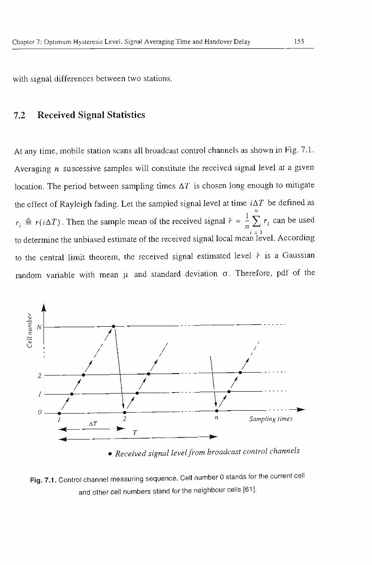
Chapter 7: Optimum Hysteresis Level, Signal Averaging Time and Handover Delay 155
with signal differences between two stations.
7.2 Received Signal Statistics
At any time, mobile station scans all broadcast control channels as shown in Fig. 7.1.
Averaging n successive samples will constitute the received signal level at a given
location. The period between sampling times AT is chosen long enough to mitigate
the effect of Rayleigh fading. Let the sampled signal level at time iAT be defined as n
r- = r(iAT). Then the sample mean of tiie received signal r = - J^ , can be used
to determine the unbiased estimate of the received signal local mean level. Accordmg
to the central limit theorem, the received signal estimated level r is a Gaussian
random variable with mean p and standard deviation a . Therefore, pdf of tiie
-a
<4j
Sampling times
Received signal level from broadcast control channels
Fig. 7.1. Control channel measuring sequence. Cell number 0 stands for the current cell
and other cell numbers stand for the neighbour cells [61].
Chapter 7: Optimum Hysteresis Level, Signal Averaging Time and Handover Delay 156
estimated signal level will be.
-{r-\lf
fdr) = -yL-e '^' (7.1) ^ 72710
7.2.1 Mean of the received signal level
Assunung all the sample signals have the same mean, r- = p,, the mean value is
given by.
r-i + r-y + ... +r„ ^^ ^^ E{r} = -^ ^ = p (7.2)
n
The mean of the signal levels received from the two base stations separated by
D[Km] at a point d[Km] from communicating base station can be formulated as,
|io( J ) = K^- K^logd d G (0, D) (7.3)
p,(^) = K^-K^logiD-d) dG (0,D) (7.4)
where K^ and K2 are the parameters representing tiie respective patii losses.
7.2.2 Variance of the received signal level
Shadowing behaves as a Gaussian noise witii an average value of zero and a standard
Chapter 7: Optimum Hysteresis Level, Signal Averaging Time and Handover Delay 157
deviation of o^. Shadowing is a slow phenomenon, having correlation effects over
several tens of meters. To model such a correlation, power spectmm of the shadow
fading S^{f) can be assumed to be flat as per [192],
S^if) = r'''^^^ '^'--^^ (7.5) lo \f\>fm
where f^ is the maximum shadow fading rate. This rate is significantly lower than
the fast fading rate (i.e. maximum Doppler rate) that would apply to the mobile
terminal's carrier envelope [193]. The auto-correlation function R^ix) of the shadow
fading signal of s{t), is derived from (7.5) and is given by:
R^(x) = S'hs.if)] = J ^'"o^/2f^ e^^^'^'df (7.6) -fn,
= a.sinc(2/„T)
where 3"^ [ ] denotes the inverse Fourier transform, and sine(X) = sin(7iX)/(7cX).
Therefore, the auto-correlation function of the received signal R^{x) and its
auto-covariance Cov{x) will be:
R(x) = RXx) + ii^ ' (7.7)
= a^sinc(2/^T) + p^
Cov{x) = a\inc(2/^T) (7.8)
Chapter 7: Optimum Hysteresis Level, Signal Averaging Time and Handover Delay 158
The variance of the mean received signal will be:
Var{r} = Varl V r-/n -i= 1
n
n
- n n •
-j = 1 J = 1 J
n -a
U = 1
1
n n
n n = y^Y.'^ar{ri)^-2^ ^ Cov{r,r.)
i = Ij = i + I 'i= 1
= 1| Cov{0) + 2 X I 1 - ^ p^( ' ' ^^) ^ J = 1
(7.9)
Using (7.8), tiie variance of tiie mean received signal can be expressed as:
Var{r} = i = 1
l + 2 y , l - - k i n c ( 2 / ^ / A r ) (7.10)
Thus the standard deviation of tiie received signal o depends on tiie number of
samples n and the time between two successive samples AT and can be obtained as.
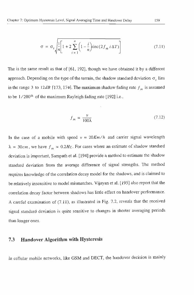
Chapter 7: Optimum Hysteresis Level, Signal Averaging Time and Handover Delay 159
n
l+2X(l-^)inc(2/^/Ar) i= 1
(7.11)
The is the same result as that of [61, 192], though we have obtained it by a different
approach. Depending on the type of the terrain, the shadow standard deviation a^ lies
in the range 3 to 12dB [173, 174j. The maximum shadow fading rate / ^ is assumed
to be 1 /200* of the maximum Rayleigh fading rate [192] i.e.,
f = —IL- (7.12) • '" 100>«
In the case of a mobile with speed v = 20Km/h and carrier signal wavelength
X = 30cm, we have f = 0.2Hz. For cases where an estimate of shadow standard
deviation is important, Sampath et al. [194] provide a method to estimate the shadow
standard deviation from the average difference of signal strengths. The metiiod
requires knowledge of the correlation decay model for the shadows, and is claimed to
be relatively insensitive to model mismatches. Vijayan et al. [195] also report that the
correlation decay factor between shadows has littie effect on handover performance.
A careful examination of (7.11), as illustrated in Fig. 7.2, reveals that the received
signal standard deviation is quite sensitive to changes in shorter averaging periods
than longer ones.
7.3 Handover Algorithm with Hysteresis
In cellular mobile networks, like GSM and DECT, the handover decision is mainly
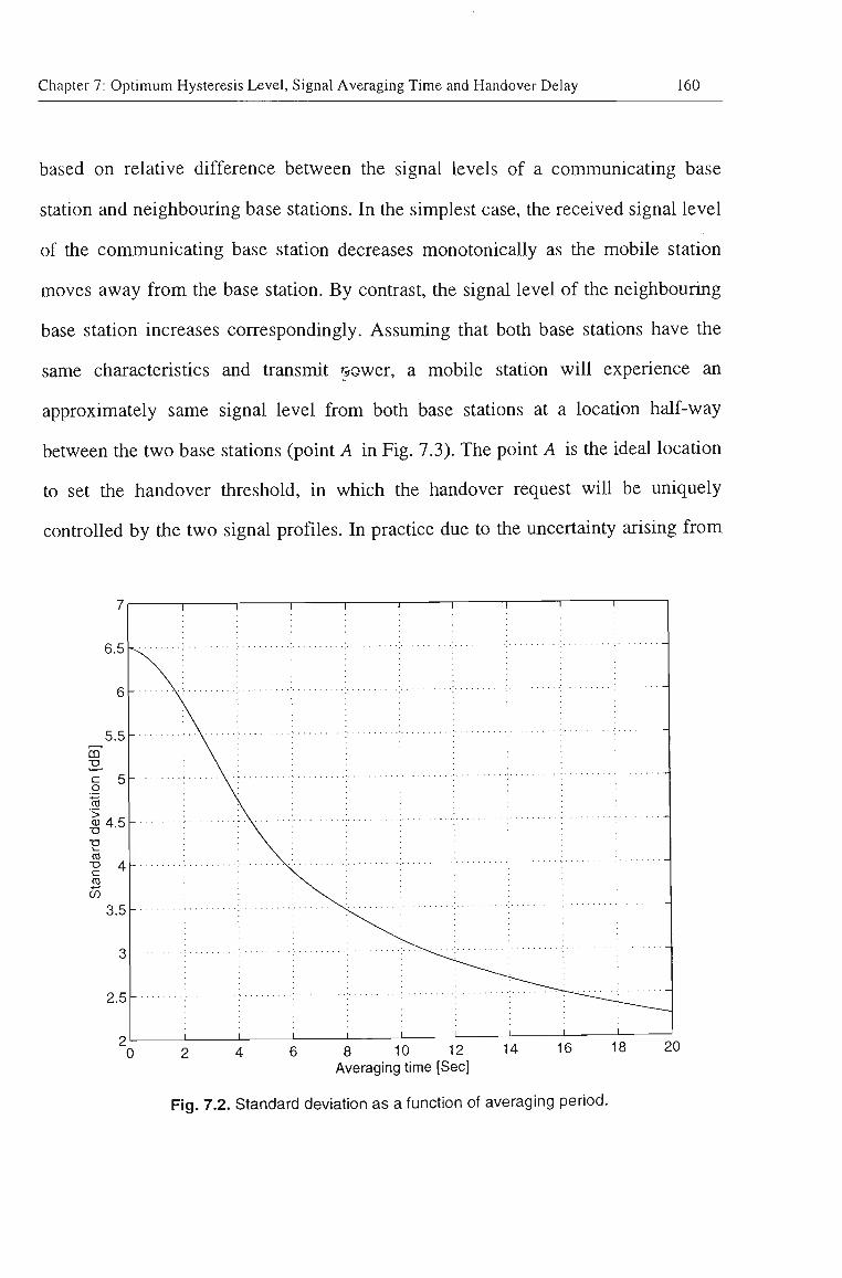
Chapter 7: Optimum Hysteresis Level, Signal Averaging Time and Handover Delay 160
based on relative difference between the signal levels of a communicating base
station and neighbouring base stations. In the simplest case, the received signal level
of the communicating base station decreases monotonically as the mobile station
moves away from the base station. By contrast, the signal level of the neighbouring
base station increases correspondingly. Assuming that both base stations have the
same characteristics and transmit ;sower, a mobile station will experience an
approximately same signal level from both base stations at a location half-way
between the two base stations (point A in Fig. 7.3). The pomt A is tiie ideal location
to set the handover tiireshold, in which the handover request will be uniquely
controlled by the two signal profiles. In practice due to the uncertainty arising from
8 10 12 Averaging time [Sec]
14 16 18
Fig. 7.2. Standard deviation as a function of averaging period.
20
Chapter 7: Optimum Hysteresis Level, Signal Averaging Time and Handover Delay 161
the fluctuation of tiie received signals, setting such a point as the handover threshold
will give rise to a numerous amount of unnecessary handovers (ping-pong effect)
before capturing the target base station. To avoid ping-pong effect a hysteresis level
is applied for handover decision. Adoption of hysteresis level can resuh in intelligent
decisions as to determine whether and when handovers should take place. However,
applying hysteresis level h[dB] shifts tiie handover decision (threshold) from point
A, (where \JiQ{d^)-\i^{D-d^) = 0) (Fig. 7.3), to pomt B, (where
U-oid2) - ^liP^ - df) = h). It is obvious that in a uniform cellular network with
similar base stations, we will have d^ = D/2.
m
> 0)
c CD
w
c
CO
-60
-65
-70
-75
-80
-85
-90
-95
-100
-105-•"
-110 0
\ 1
- 1
1 1 1 1 1 1 1 '
: : / : / •
AverageTeceiveQ stgnai levei Trom Dtsu •; ; / . : : :/
— Average received signal level from BS1 / • •. . '• '• . . . . .'• • • / . : . •
/ : • : / . : / .:
./ _• : \ • • ^ • ' :
\ . : : : . / . •
^^^ A ^ :
.. •" ^
: di dp
6 8 10 12 14 Distance from BSO to BS1 (Km)
16 18 20
Fig. 7.3. Received signal level from two base stations without shadow fading.
Chapter 7: Optimum Hysteresis Level, Signal Averaging Time and Handover Delay 162
7.4 Unnecessary Handovers
The probability of an unnecessary handover Pu is defined as the probabtiity that a
mobile station performs a handover from the existing base station BSO to the
neighbouring base station BSl and then initiates another handover back to BSO. Let
^#0 be the signal estimated level in dB received at the mobile station from die
communicating base station, and R#i be the signal estimated level received from the
neighbouring base station which has the stiongest level among all other neighbouring
base stations. Then, the respective handover probabilities (connection from BSO to
BS 1 and back from BS I to BSO) can be defined by,
prob{BSO^BSl} = \^ prob{R#i= r}-prob{R#o<{r-h)}-dr (7.13) J 1"= —oo
prob{BSl^BSO} = f °° prob{R#o= r} • prob{k#i < {r- h)} • dr (7.14) • p'= —oo
where.
prob{Rn= r} = F^^{r + dr) - F^Jr) (7.15)
and ff, (r) has a normal pdf as in (7.1). Considering,
f(x)=i^(0.l) = f=e-''' (7.16) J2K
Chapter 7: Optimum Hysteresis Level, Signal Averaging Time and Handover Delay 163
as the normalised received signal pdf, the prob{R#\= r} will be equal to:
prob{R#i= r} = F^{x + dx) -F^{x)
= prob{X= x} (7.17)
r-p-i where, x= . The same argument wiU result in.
prob{R#o<{r-h)} = F . {r-h) " # 0
= F .
= F .
= F v U -
f-h-\iQ
r-h-\ii + AL
a h-AL
= probUX-^^yx
(7.18)
where AL = p^ - p-o is the difference between tiie two received signal levels due to
tiie patii loss difference from tiie two base stations. Considering (7.17) and (7.18), we
can replace (7.13) with tiie following relation (Fig. 7.4),
prob{BSO-^BSl} = f" prob{X= x} • probl \X ^ j < x dx
(7.19) oo ,- X
= j/w j/(-^> dx
The same procedure wiU resuh in.
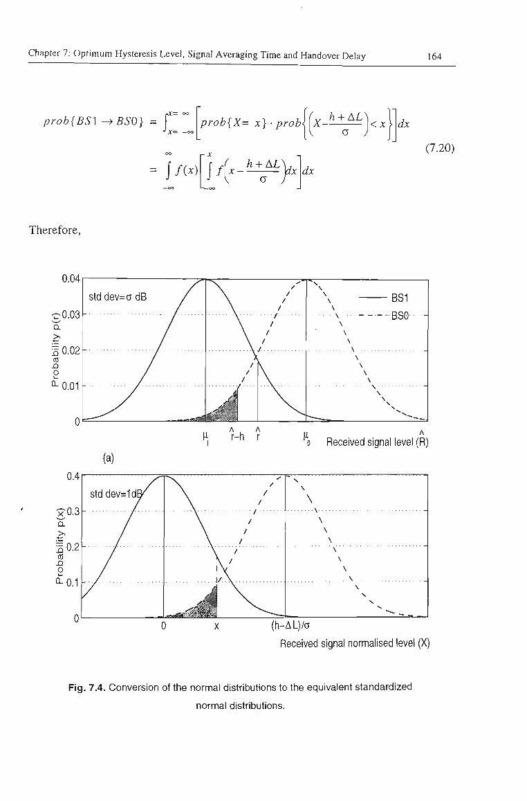
Chapter 7: Optimum Hysteresis Level, Signal Averaging Time and Handover Delay 164
prob{BS\ -^BSO} = f prob{X= x} • probl I X-^^-^^\<x dx
°° r- X (7.20)
dx
Therefore,
(a)
0.4
0.3
10.2 CO n o D O.1
tl ^ 0 Received signal level (R)
stddev=1dB^ \ /
\ / \ /
V / \ / \ / \ /
' \ l / . \
s \
\ \ \ \ \
\ .. N _
\ \
(h-AL)/a
Received signal normalised level (X)
Fig. 7.4. Conversion of the normal distributions to the equivalent standardized
normal distributions.
Chapter 7: Optimum Hysteresis Level, Signal Averaging Time and Handover Delay 165
°° r- X -J oo _ JC
= j /w •1 J h-AL\ dxx { f{x)
<7 J
h + AL\
dx
- + erf\x-2 V a ; j
dx
(7.21)
where, erf{x) = j/(j:)(iA;. This re':ult agrees witii that of [61], where it was stated
without proof. The closed-form solution of (7.21) is difficult and a numerical
integration performed within the limits of ±3 a for different values of AL and h
gives the results illustrated in Fig. 7.5. It can be seen that the probability of
unnecessary handovers is maximum when a mobile station is moving on the cell
boundary, i.e. AL = 0.
A numerical solution of (7.11), (7.21) could explain tiie dependencies between
standard deviation of the sample averaged received signal a , standard deviation of the
shadow fading c^, received signal averaging time T, hysteresis level h and
unnecessary handover probability Pfj. Fig. 7.6 shows tiie variation of unnecessary
handover probability witii the averaging time, for two different hysteresis levels. It is
clear from the figures tiiat tiiis probability decreases rapidly witii increasing
averaging time. The amount of averaging time required to reduce inappropriate
handover requests is dependent on the variance of shadow fading to which the signal
is subjected. Under light shadowing conditions (less variance) the handover
algorithm performs better witii low values of hysteresis levels. In tiiis situation a high
hysteresis level could extend the cell boundary beyond acceptable limits, causing
both cochannel and adjacent channel interference in neighbouring ceUs. The same
results have been extracted by Dassanayake [56] via simulation.
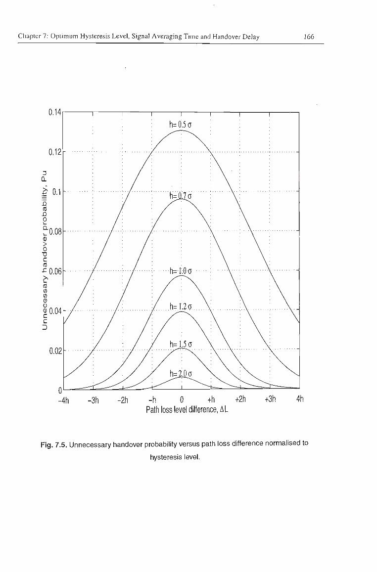
Chapter 7; Optimum Hysteresis Level, Signal Averaging Time and Handover Delay 166
-4h -3h -2h -h 0 +h +2h +3h 4h Path loss level difference, AL
Fig. 7.5. Unnecessary handover probability versus path loss difference normalised to
hysteresis level.
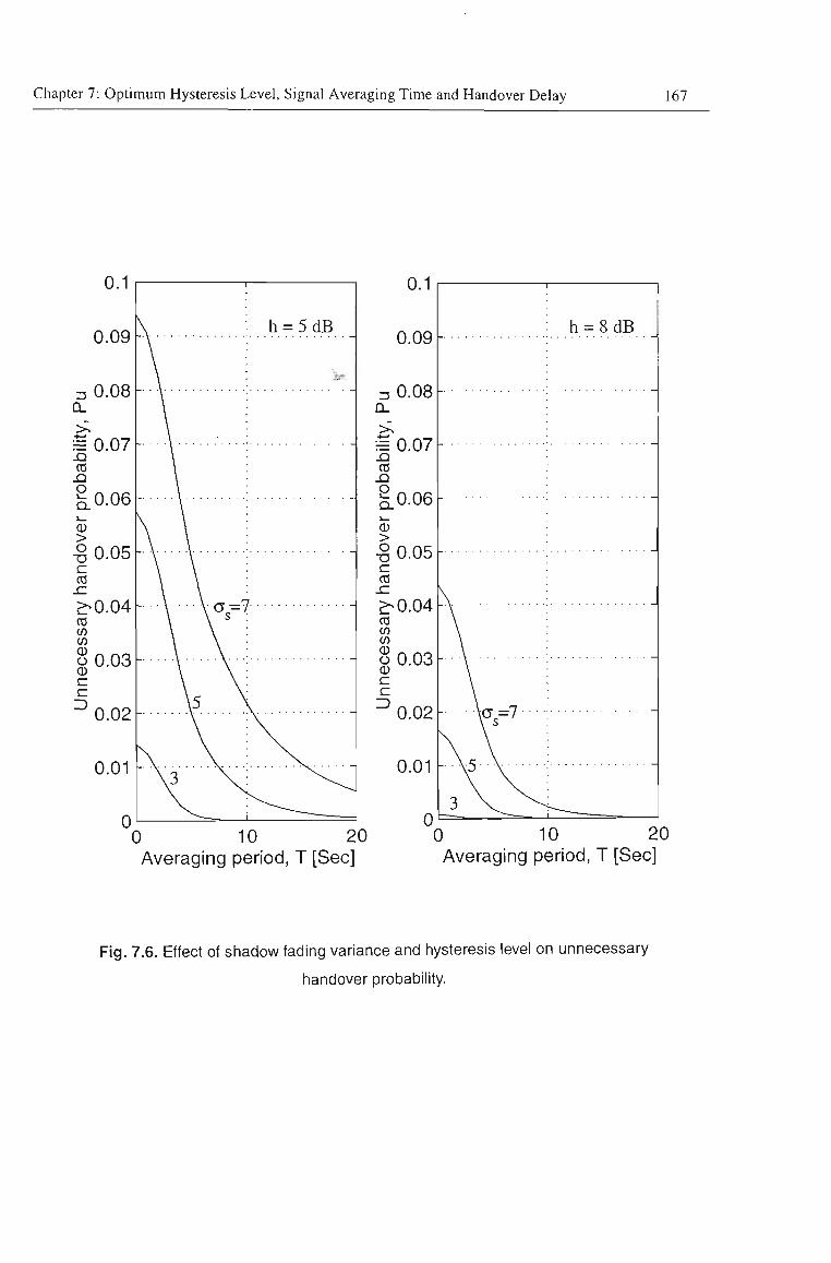
Chapter 7: Optimum Hysteresis Level, Signal Averaging Time and Handover Delay 167
0.1
0.09
5 0 . 08 Q. >^ = 0.07 sn CO
1.0.06 a>
-§0.05 c CO x: >^0.04 CO w V)
S0.03 CD C
c ^0 .02
0.01 -
0
-•• y-W'
V . y \ 3 \
h = 5dB
» ? ,
J
0.1
0.09
3 0.08 Q_
1=0.07 XI CO
§.0.06
I 0.05 c CO
^0.04 CO CO
§0.03 CD c c -^0.02
0.01
0 10 20 Averaging period, T [Sec]
0
\rt- 1 . . .
- As V -1 v _ ^
h = 8dB
-
0 10 20 Averaging period, T [Sec]
Fig. 7.6. Effect of shadow fading variance and hysteresis level on unnecessary
handover probability.
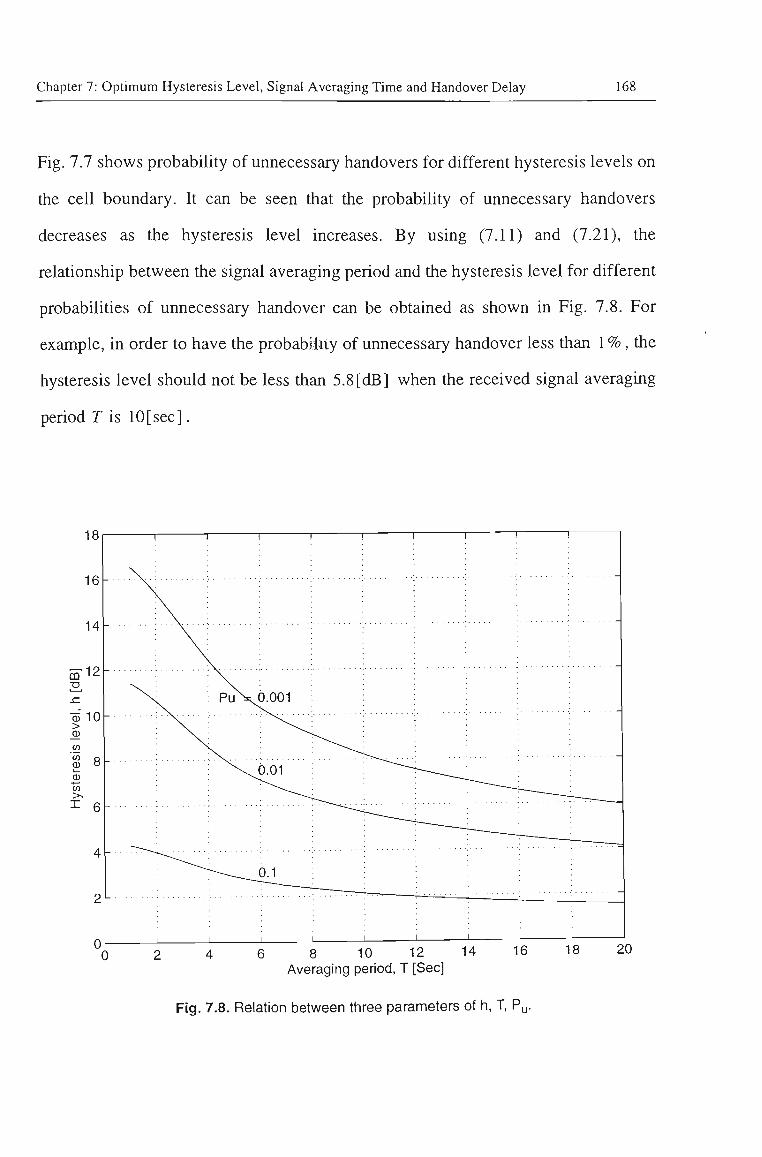
Chapter 7: Optimum Hysteresis Level, Signal Averaging Time and Handover Delay 168
Fig. 7.7 shows probability of unnecessary handovers for different hysteresis levels on
the cell boundary. It can be seen that the probability of unnecessary handovers
decreases as the hysteresis level increases. By using (7.11) and (7.21), the
relationship between the signal averaging period and the hysteresis level for different
probabilities of unnecessary handover can be obtained as shown in Fig. 7.8. For
example, in order to have the probability of unnecessary handover less than 1 %, the
hysteresis level should not be less than 5.8[dB] when the received signal averaging
period F is 10[sec].
6 8 10 12 14 Averaging period, T [Sec]
16 20
Fig. 7.8. Relation between three parameters of h, T, Pu-
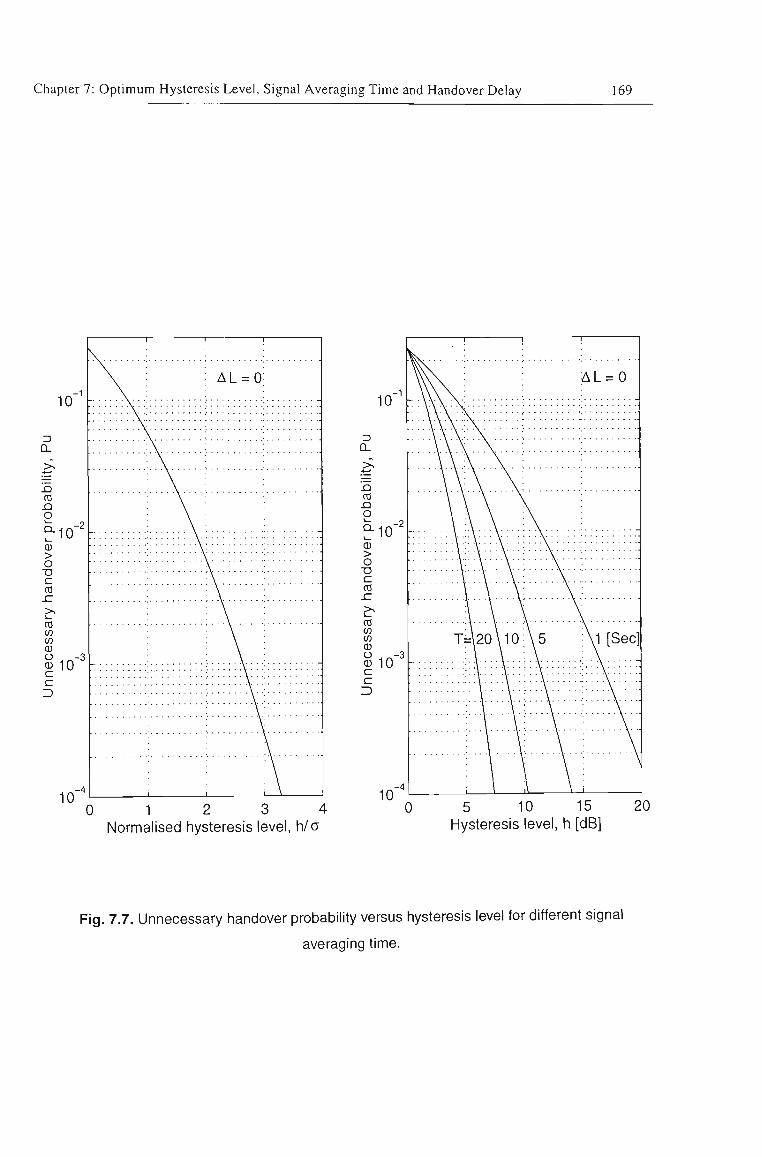
Chapter 7: Optimum Hysteresis Level, Signal Averaging Time and Handover Delay 169
0 1 2 3 4 Normalised hysteresis level, h/a
5 10 15 Hysteresis level, h [dB]
Fig. 7.7. Unnecessary handover probability versus hysteresis level for different signal
averaging time.
Chapter 7: Optimum Hysteresis Level, Signal Averaging Time and Handover Delay 170
7.5 Handover Delay
Handover delay is another issue of concem in the design of handover algorithms. If
handover does not occur quickly, the quahty of service (QoS) may deteriorate below
an acceptable level. Minimizing delay also minimizes co-channel interference. If tiie
signal quahty changes fast the handover algorithm must react promptiy hr order to
save the call. The time involved in the handover process is mainly due to the time
taken for measuring and processing the signal strength, and making a decision for
handover initiation, if actual switching time is ignored.
One other consideration that has to be taken into account when designing handover
schemes is that fast handover algorithms can be unstable, while slower handover
algorithms can result in poor signal quality. Unstable handover schemes consume a
lot of computational resources just for handover management; resources that could
be better used for other tasks. A slow algorithm can cause a mobile to remain
connected to a base station even when it has moved well inside the cell of a closer
base station.
The handover delay can be taken as the time delay occurring due to signal averaging
and setting of a hysteresis margin. The averaging period T includes n samples with
half of them extracted from the past samples. Therefore, the averaging would create a
constant delay of F / 2 . Moreover, applying hysteresis level causes an additional
delay. Hysteresis delay 5 ^ is defined as the time associated between optimal point of
handover and the actual point of handover with hysteresis. The optimal point (or
crossover point) is the point where the probability of mobile being assigned to either
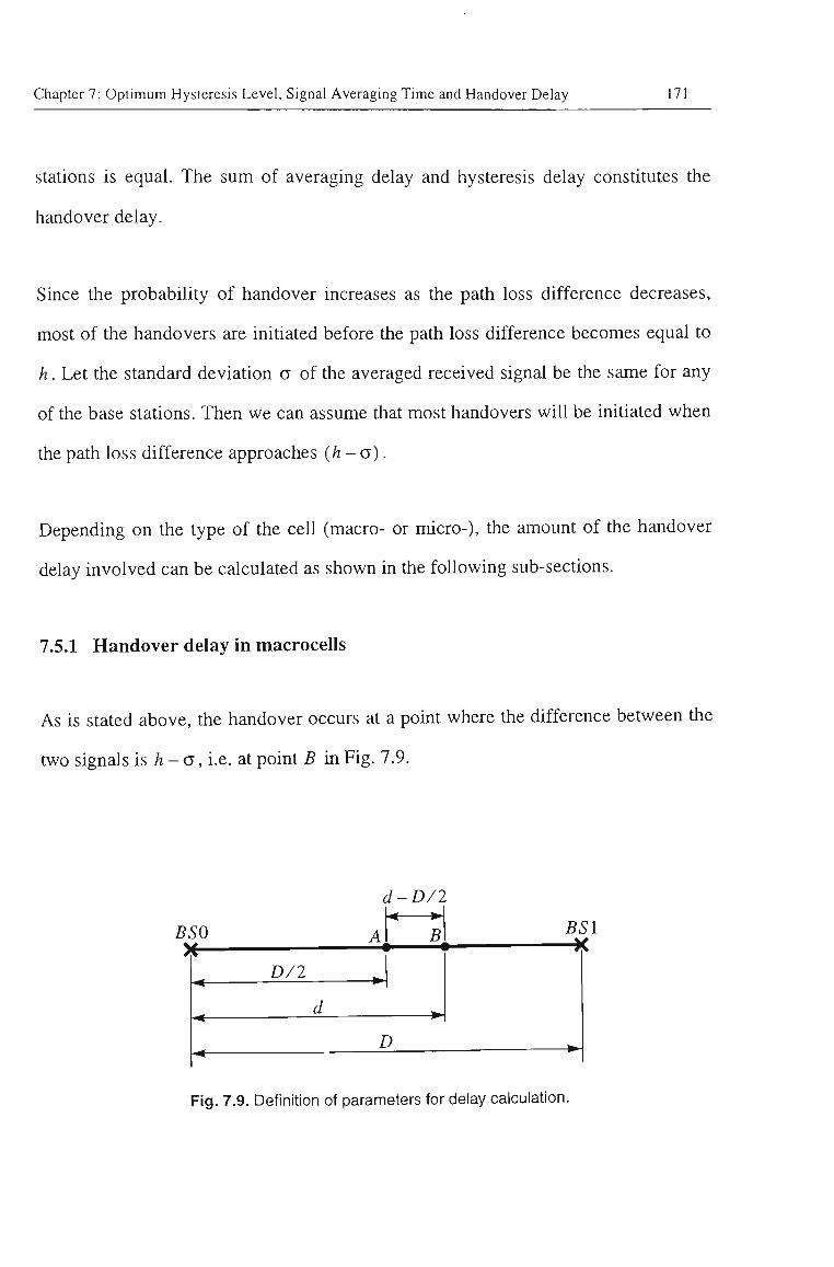
Chapter 7: Optimum Hysteresis Level, Signal Averaging Time and Handover Delay 171
Stations is equal. The sum of averaging delay and hysteresis delay constitutes the
handover delay.
Since the probability of handover increases as the path loss difference decreases,
most of the handovers are initiated before the path loss difference becomes equal to
h. Let the standard deviation a of the averaged received signal be the same for any
of the base stations. Then we can assume that most handovers will be initiated when
the path loss difference approaches {h-o).
Depending on the type of the cell (macro- or micro-), the amount of tiie handover
delay involved can be calculated as shown in the following sub-sections.
7.5.1 Handover delay in macrocells
As is stated above, the handover occurs at a point where tiie difference between tiie
two signals is h-a, i.e. at point B in Fig. 7.9.
BSO
D/2
d-D/2 < >-
B
D
BSl
Fig. 7.9. Definition of parameters for delay calculation.
Chapter 7: Optimum Hysteresis Level, Signal Averaging Time and Handover Delay 172
/ z - a = P i - P o (7.22)
Let d be the distance of handover point from the BSl, and D be the distance
between two base stations as shown in Fig. 7.9. Using (7.3) and (7.4), with (7.22) the
hysteresis margin can be obtained as follows.
h-<5 = K^^log D-d
(7.23)
Therefore,
h-(5
^ =10"' D-d
(7.24)
After some algebraical manipulation the following relation can be obtained.
2d-D D
10 "" - 1
h-a
/ I 10 ^ ' + 1 (7.25)
A mobile moving at a speed v will be subjected to a delay in handover decision
making which (from Fig. 7.9) can be calculated as the time interval associated
between points A and 5 . Therefore, handover delay is.
h = d-D/2 (7.26)
Chapter 7: Optimum Hysteresis Level, Signal Averaging Time and Handover Delay 173
Considering (7.25) and (7.26) we have,
^^ = £l 10
h-o ~K7
/ 10
/ x - g
-Hi (7.27)
This result is similar to that of [61], where it was stated without proof. Let the cell
size be normalized with respect to the speed of the mobile and be shown by
Kj^^ = D /2v . Then the total handover delay in a macroceU 6 ^ witi be:
^hM - 2 """ ^^^"1 10
h-o ~K7
- 1 / 10
h-o
+ 1 (7.28)
Fig. 7.10 illustrates the handover delay as a function of hysteresis for different values
of signal averaging period and normalized cell size, Kj^^. It can be seen that tiie
handover delay and tiie hysteresis level are linearly related to each other. The
proportionality factor (i.e. the increase in handover delay for an increase in hysteresis)
increases with increasing normalized cell size. This is because tiie path loss slope
near the ceU boundaries decreases as the cell radius increases.
The delay in handover for a given probability of unnecessary handover increases as
the hysteresis level increases and the averaging period decreases. Therefore, in case
of macrocells where Kj^^ is large, it is preferable to have a longer averaging period
and smaller hysteresis level. This phenomenon is shown in Fig. 7.11. Since any
change in the speed of tiie mobtie will vary Kj^^, it is best to choose velocity adaptive
signal averaging intervals. Different velocity estimators have been suggested in [4,
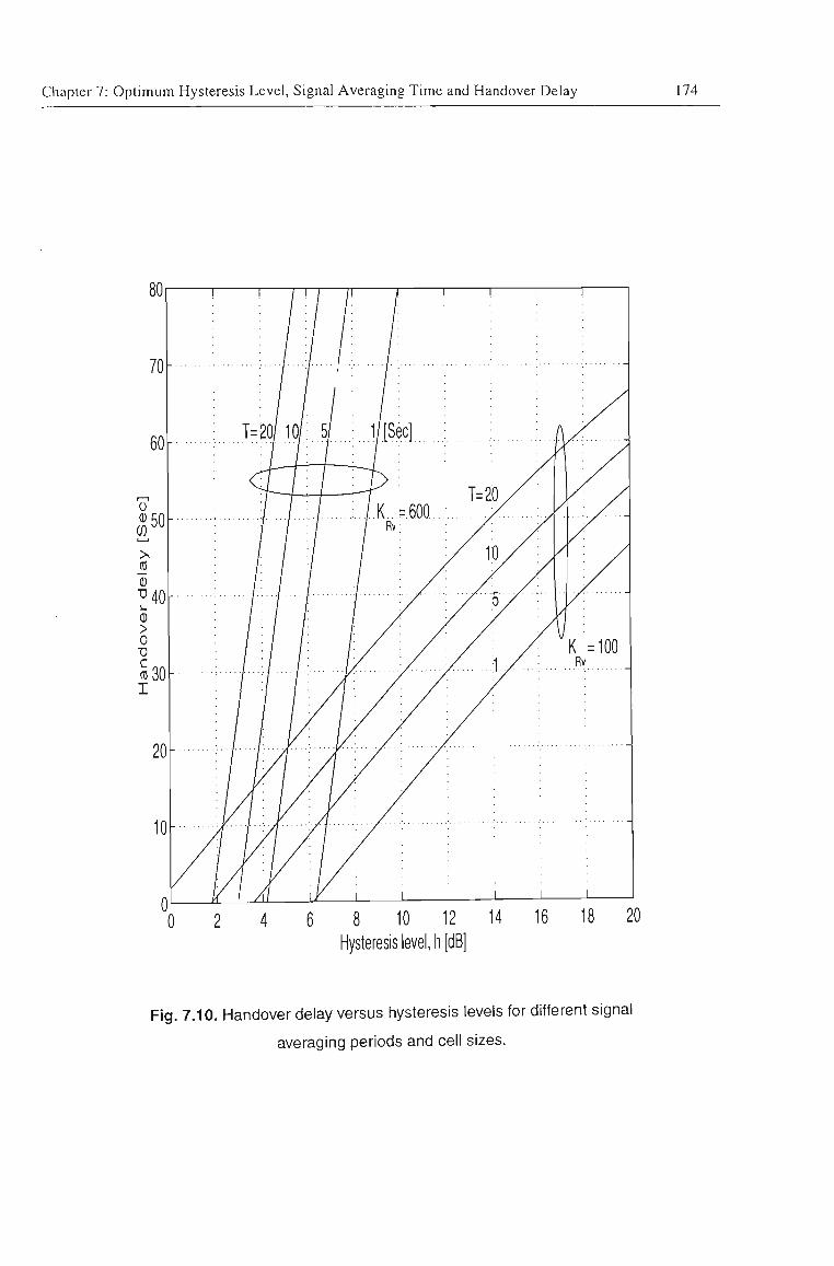
Chapter 7: Optimum Hysteresis Level, Signal Averaging Time and Handover Delay 174
0 2 4 6 8 10 12 14 16 18 20 Hysteresis level, h [dB]
Fig. 7.10. Handover delay versus hysteresis levels for different signal
averaging periods and cell sizes.
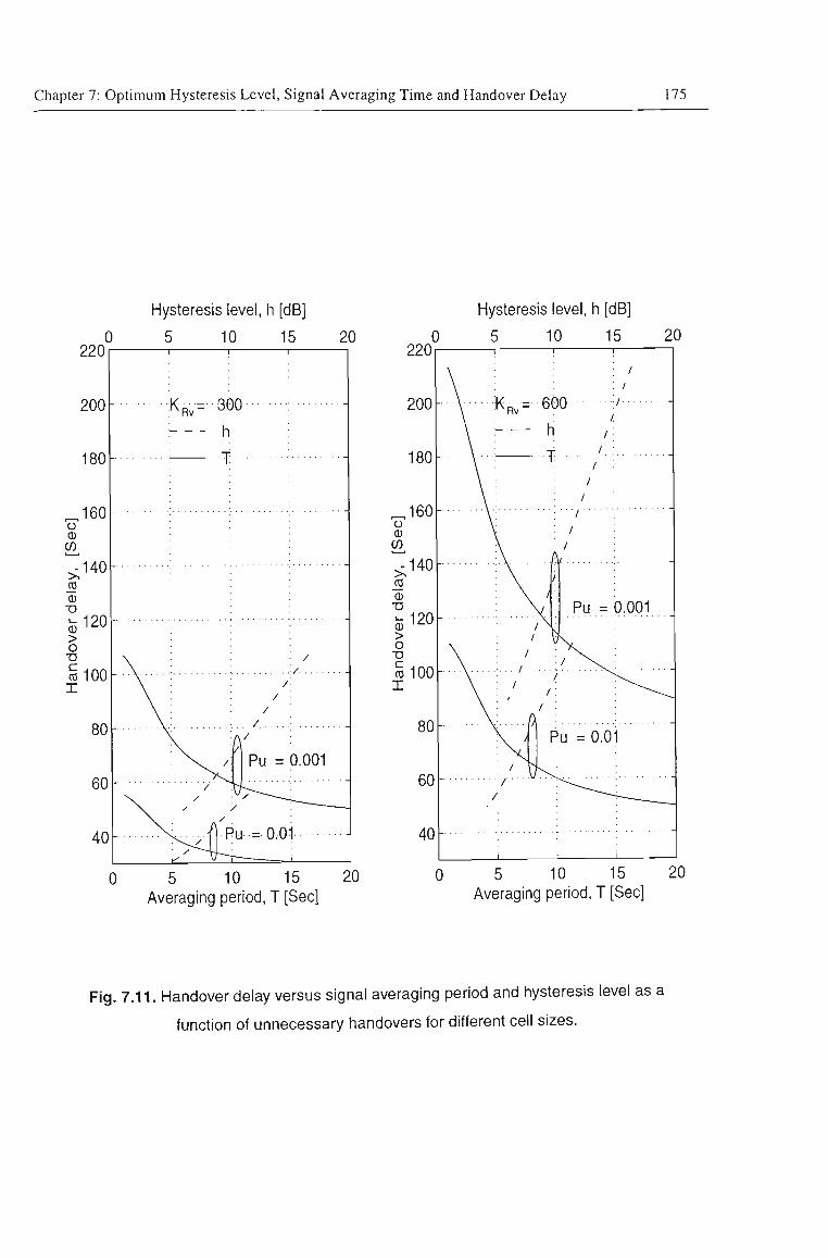
Chapter 7: Optimum Hysteresis Level, Signal Averaging Time and Handover Delay 175
Hysteresis level, h [dB] Hysteresis level, h [dB]
10 15 20 10 15 20
0 5 10 15 20 Averaging period, T [Sec]
0 5 10 15 20 Averaging period, T [Sec]
Fig. 7.11. Handover delay versus signal averaging period and hysteresis level as a
function of unnecessary handovers for different cell sizes.
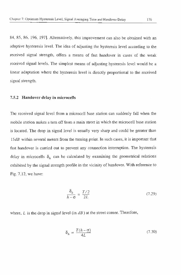
Chapter 7: Optimum Hysteresis Level, Signal Averaging Time and Handover Delay 176
84, 85, 86, 196, 197]. Alternatively, this improvement can also be obtained with an
adaptive hysteresis level. The idea of adjusting the hysteresis level according to the
received signal strength, offers a means of fast handover in cases of tiie weak
received signal levels. The simplest means of adjusting hysteresis level would be a
linear adaptation where the hysteresis level is directly proportional to the received
signal strength.
7.5.2 Handover delay in microcells
The received signal level from a microcell base station can suddenly fall when the
mobile station makes a turn off from a main street in which the microcell base station
is located. The drop in signal level is usually very sharp and could be greater than
15dB within several meters from the tuming point. In such cases, it is important that
fast handover is carried out to prevent any connection intermption. The hysteresis
delay in microcells 6; can be calculated by examining the geometrical relations
exhibited by the signal strength profile in the vicinity of handover. With reference to
Fig. 7.12, we have:
h T/2 . 29) h-G 2L
where, L is the drop in signal level (in dB) at the street comer. Therefore,
5 = T(h-o) (7 30) " 4L
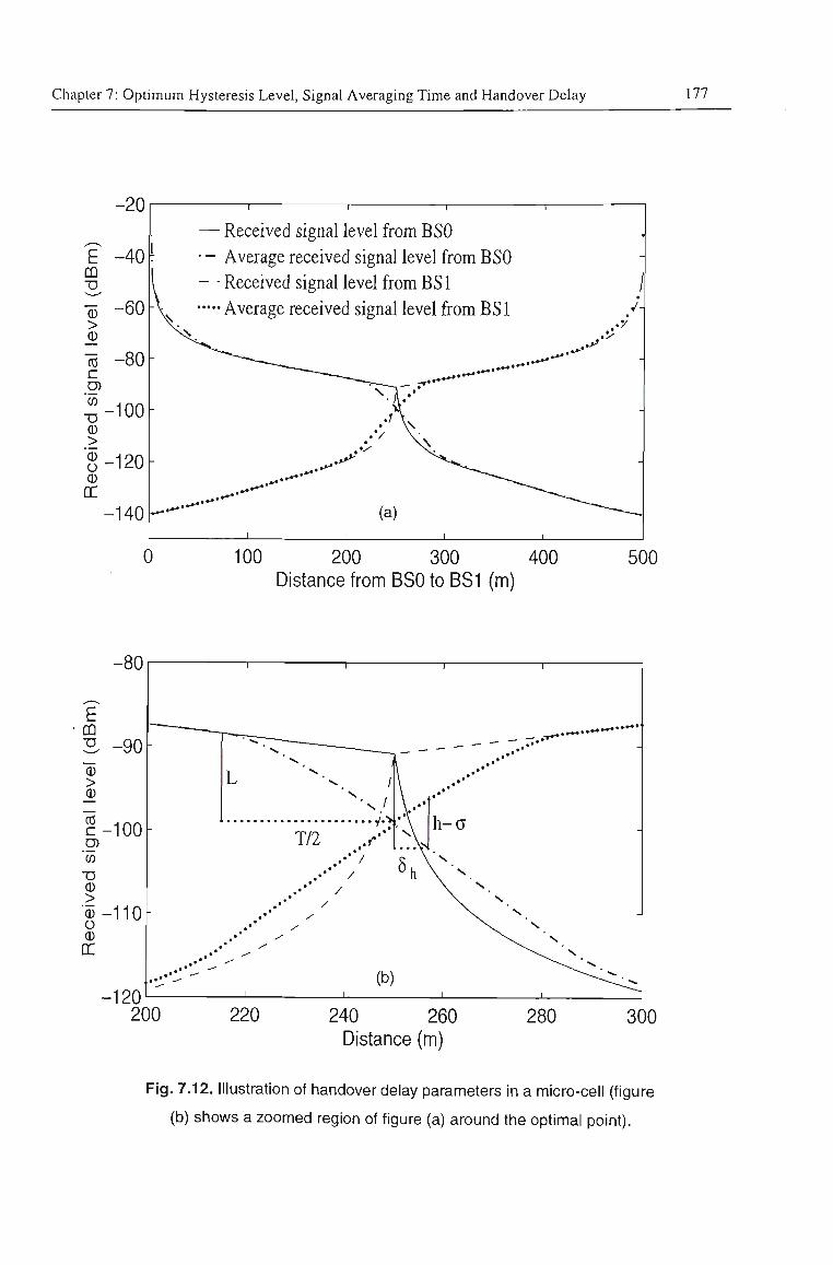
Chapter 7: Optimum Hysteresis Level, Signal Averaging Time and Handover Delay 177
CD
> .0) "cO c
'(/) T3 • (D >
"(D o • CD
-c\j
-40
-60
-80
100
120
140
1 1 1 1
— Received signal level from BSO : • - Average received signal level from BSO 1 - - Received signal level from BSl -V Average received signal level from BS 1
. • • ' \
(a) 1 1 1 r
fl
-
/ •
•
. . . • ' • '
.*••
-
-
^ ^ ^
0 100 200 300 400 Distance from BSO to BSl (m)
500
-80
E CQ
S -90
>
?-100 D) '(0 T3 (D
1-110 o (D d
-120 200
1 1 -
• ^ — '
>s
L s
T/2 ..•
.'• / .••' /
/ y
y y
.* y --
1 1
1 1
/
> s /
. ^ • •
• • • • • \ V'"* .•"\
N \ h-a
' 5A-X \ s
\ ^ \ \^^ N
\ , . ^ N \ ~ ^ S
^ ^ ^ ^ ^ N ^^---^^' V
(b) ^--^ : : :L: :^ 1 1
220 240 260 Distance (m)
280 300
Fig. 7.12. Illustration of handover delay parameters in a micro-cell (figure
(b) shows a zoomed region of figure (a) around the optimal point).
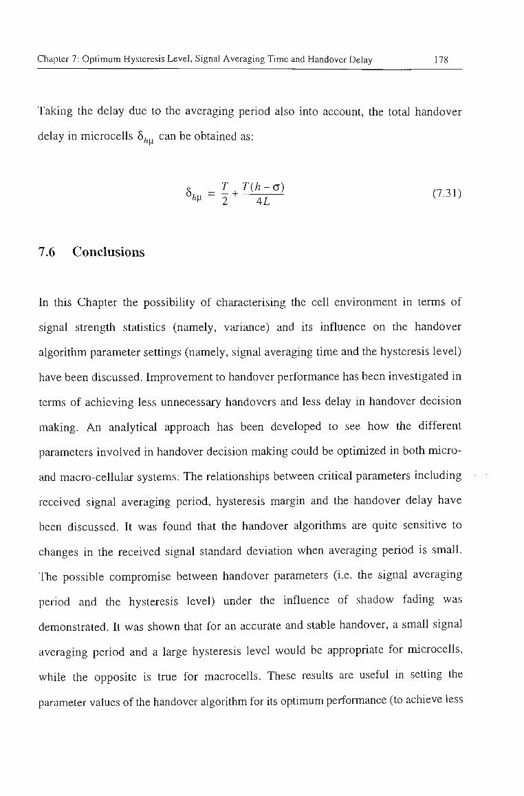
Chapter 7: Optimum Hysteresis Level, Signal Averaging Time and Handover Delay 178
Taking the delay due to the averaging period also into account, the total handover
delay in microcells 6; , can be obtained as:
8 , , = ! + ^ ^ (7.31)
7.6 Conclusions
In this Chapter the possibility of characterising the cell environment in terms of
signal strength statistics (namely, variance) and its infiuence on the handover
algorithm parameter settings (namely, signal averaging time and the hysteresis level)
have been discussed. Improvement to handover performance has been investigated in
terms of achieving less unnecessary handovers and less delay in handover decision
making. An analytical approach has been developed to see how the different
parameters involved in handover decision making could be optimized in both micro-
and macro-cellular systems. The relationships between critical parameters including
received signal averaging period, hysteresis margin and the handover delay have
been discussed. It was found that the handover algorithms are quite sensitive to
changes in the received signal standard deviation when averaging period is small.
The possible compromise between handover parameters (i.e. the signal averaging
period and tiie hysteresis level) under the influence of shadow fading was
demonstrated. It was shown that for an accurate and stable handover, a small signal
averaging period and a large hysteresis level would be appropriate for microcells,
while the opposite is tme for macrocells. These results are useful in setting the
parameter values of the handover algorithm for its optimum performance (to achieve less
Chapter 7: Optimum Hysteresis Level, Signal Averaging Time and Handover Delay 179
delay in handover decision making and less unnecessary handovers). The results also
suggest that a hybrid handover algorithm with microcell and macrocell sensors could be
used to achieve optimum performance. When the macrocell sensor is triggered a long
averaging period and a short hysteresis level should be selected, while the reverse
should occur when the microcell sensor is triggered.
In order to account for the velocity, it is best to choose velocity adaptive signal
averaging intervals. This improvement can also be obtained with an adaptive
hysteresis level. The idea of adjusting the hysteresis level according to tiie received
signal strength offers a means of fast handover in cases of weak received signal
levels.
Chapter 8
Conclusions
In this thesis, three important issues related to the handover process of cellular
mobile systems have been investigated. They are the foUowing,
• Effect of mobility on handover,
• Effect of handover on teletraffic performance criteria,
• Effect of propagation environment on handover decision making.
The results of this thesis are apphcable to any analogue or digital cellular system in
which the concept of channel is applicable.
Chapter 8: Conclusions 181
8.1 Effect of mobility on handover
In Chapter 3 a mathematical formulation has been developed for systematic tracking
of the random movement of a mobile station in a cellular environment. It
incorporates mobility parameters under most generalized conditions so that the
model could be tailored to be applicable in most cellular systems. The proposed
model traces mobiles systematically in a cellular environment where they are
allowed to move in a quasi-random fashion with assigned degrees of freedom. It
enables the development of a computer simulation to investigate the characteristics
of different mobility related traffic parameters in a cellular system. These parameters
include the distribution of the cell residence time of both new and handover calls,
channel holding time and the average number of handovers per call. Results show
that the generalized gamma distribution is adequate to describe the cell residence
time distribution of both new and handover caUs. Results also show that the negative
exponential distribution is a good approximation for the channel holding time
distribution in cellular mobile systems. In order tiiat tiiese results could be made
applicable to a wide range of cellular environments, it was shown that any velocity
change in tiie mobile in a cell can be tieated as contributing to an effective change in
the cell radius. Taking tiiis excess ceU radius that corresponds to different values of
velocity into account, a broad variety of cell coverage areas with different street
orientations and traffic flows can be handled.
Further investigation is proposed to extend tiiis method to cover the cases of
microcells (CBD street stmctures witii traffic light effects) and picocells (in-building
3D structures with slow motion).
Chapter 8: Conclusions 182
8.2 Effect of handover on teletraffic performance criteria
In Chapter 5, different radio resource allocations were explained, teletiaffic
performance criteria were defined and an analytical model for teletraffic performance
evaluation was presented. Also some traffic policies that give a higher level of
protection to handover calls we-e described and their effect on the overall tiaffic
performance were analysed. Based on the results obtained for cell residence time
distribution, a teletraffic model tiiat takes the user mobihty into account has been
presented and substantiated using a computer simulation using the next-event
time-advance approach. Furthermore, tiie influence of cell size on new and handover
call blocking probabilities has been examined. The effect of the handover channel
reservation on call dropout probability has been investigated to determme the
optimum number of reserved channels required for handover.
It was found that blocking probabilities of new and handover calls are tiie same when
tiiere are no reserved channels for tiie handover calls. However, tiiese blocking
probabilities become different when a portion of channels are reserved for handover
calls. The rate of change of blocking probabilities of tiie new and handover calls witii
tiie number of reserved channels is such tiiat tiie decrease in blocking probability of
the handover calls due to an increase in the number of reserved channels is
significantiy bigger tiian tiie corresponding increase in tiie blocking probability of
new calls. This is what makes tiie reserved channel scheme attiactive. An efficiency
factor was defined to estimate tiie effectiveness of tiiis scheme. It was found tiiat the
scheme is most efficient when traffic is heavy and handover calls are most likely to
be blocked.
Chapter 8: Conclusions 183
It was also shown that with increasing cell radius, blocking probability approaches
the Erlang-B resuhs. Furthermore, the variation of the blocking probabtiity witii
effective offered traffic per cell is independent of the cell size and is equal to
Erlang-B results. This means that for a given new call arrival rate tiie consequent
effective traffic intensity in a cell remains constant and is independent of ceU size.
It was also shown that the dropout probabihty decreases with increasing number of
reserved channels. This reduction is paid for by an increase in new call blocking
probability. A compromise between the new call blocking probability and the
dropout probability could be estabhshed by allocating a threshold level on the
dropout probability.
8.3 Effect of propagation environment on handover decision making
In Chapter 6, the contributions of the three different components of the mobile radio
signal were considered, and propagation models suitable for micro- and macro-cells
were presented. Emphasis was made on the effect of shadow fading which is by far
the most important component in handover decision making in cellular networks. It
was shown how a simple AR-1 model could be implemented using a digital filter to
simulate the shadow fading component of the signal.
In Chapter 7, the possibility of characterising the cell environment in terms of signal
strength statistics (namely, variance) and its influence on the handover algorithm
parameter settings (namely, signal averaging time and the hysteresis level) have been
discussed. Improvement to handover performance has been investigated in terms of
Chapter 8: Conclusions 184
reductions in unnecessary handovers and handover delay time. An analytical
approach has been developed to see how the different parameters involved in
handover decision making could be optimized for both micro- and macro-cellular
systems. The relationships between critical parameters including the received signal
averaging period, the hysteresis level and the handover delay have been discussed.
It was found that the handover algorithms are quite sensitive to changes in the
received signal standard deviation when averaging periods are small. The possible
compromise between handover parameters (i.e. the signal averaging period and the
hysteresis level) under the influence of shadow fading has been demonstrated. It was
shown that for an accurate and stable handover, a small signal averaging period and a
large hysteresis level would be appropriate in microcells, while the reverse would be
true in macroceUs. These results could be used in setting tiie parameters of the
handover algorithm to achieve less delay in handover decision making and less
unnecessary handovers. A hybrid handover algoritiim witii microcell and macrocell
sensors could be used for optimum decision making such tiiat when tiie macrocell
sensor is triggered a long averaging period and a short hysteresis are chosen while the
opposites are chosen when microceU sensor is tiiggered. In order to account for the
velocity, it is best to choose velocity adaptive signal averaging intervals. This
improvement can also be obtained with adaptive hysteresis levels. The idea of
adjusting the hysteresis level according to the received signal strength offers a means
of adopting fast handover in situations where received signal falls below the nominal
levels.
References
[1] V. H. MacDonald, "Advanced mobile phone service: The cellular concept," The Bell System Technical Journal, vol. 58, no. 1, pp. 15-41, Jan. 1979.
[2] Bell System, "Advanced mobile phone service," The Bell System Technical Journal (special issue), vol. 58, no. 1, Jan. 1979.
[3] F. H. Blecher, "Advanced mobile phone service," IEEE Transactions on Vehicular Technology, vol. 29, no. 2, pp. 238-244, May 1980.
[4] W. C. Jakes, Microwave Mobile Communications. New York: John Wiley and Sons, 1974.
[5] M. Mouly and M. B. Pautet, The GSM system for mobile communications. France: Mouly, Palaiseau, 1992.
[6] D. J. Goodman, "Second generation wireless information networks," IEEE Transactions on Vehicular Technology, vol. 40, no. 2, pp. 366-374, May 1991.
[7] K. Kinoshita, M. Kuramoto and Nakajima, "Development of a TDMA digital cellular system based on Japanese standard," 4Ist. IEEE Vehicular Technology Conference (VTC'9I), St. Louis, pp. 642-645, May 1991.
[8] TIA/EIA IS54, "Digital system dual-mode mobile station base station compatibility standard," Technical report 80-7814 Rev DCR 03567, Apr. 1992.
[9] Qualcomm Inc., "An overview of the application of code division multiple access (CDMA) to digital cellular systems and personal cellular network," Technical report EX60-10010, May 1992.
[10] A. Salmasi and K.S. Gilhousen, "On the system design aspects of code division multiple access (CDMA) and personal conununications networks," 41st IEEE
References 186
Vehicular Technology Conference (VTC'91), St. Louis, pp. 57-62, May 1991.
[11] Steedman, "The common air interface MPT 1375," Cordless Telecommunications in Europe, W.H. W. Tuttiebee, ed.. Springer Verlag, 1990.
[12] ETSI, Digital European Cordless Telecommunications-Common interface, Version 05.03, May 1991.
[13] K. Ogawa, K. Kohiyama and T. Kobayashi. "Towards the personal communication era- a proposal of the radio access concept from iapan," Intemational Journal Wireless information networks, vol. 1, no 1, pp. 11-2.1, Jan. 1994.
[14] Research and development centre for radio systems (RCR), "Personal handy phone systems," RCR STD-28, Dec. 1993.
[15] Bellcore, "Generic criteria for version 0.1 wireless access communications systems (WACS) and supplement," Bellcore, Tech. Rep. TR-INS-001313, issue 1, 1994.
[16] D. C. Cox, "Wireless network access for personal communications," IEEE Communications Magazine, vol. 30, no. 12, pp. 96-115, Dec. 1992.
[17] ANSI J-STD, "Personal access communication system air interface standard," 1995
[18] D. C. Cox, "Personal communications-A viewpoint," IEEE Communications Magazii^e, vol. 128, no. 11, pp. 8-20, Nov. 1990.
[19] J. E. Padgett, C. G. Giinther and T. Hattori, "Overview of wireless personal communications," IEEE Communications Magazine, vol. 33, no. 1, pp. 28-41, Jan. 1995.
[20] F Abrishamkar and E. Biglieri, "An Overview of wireless communications," IEEE Military Communications Conference, (MILCOM'94), Fort Monmouth, NJ, pp. 900-905, Oct. 1994.
[21] L. Grubb, "The travellers dream come tme," IEEE Communication Magazine, vol. 29, no. 11, pp. 48-51, Nov. 1991.
[22] J. C. B. Dende, R. Nevoux and J.C. Dang, "Networks, users and terminals in UMTS/FPLMTS," IEEE Transactions on Vehicular Technology, vol. 43, no. 3, pp. 681-685, Aug. 1994.
[23] J. M. Nijhof, L S. Dewantara and R. Prasad, "Base station system configurations
References 187
for third generation mobile telecommunication systems," 43rd. IEEE Vehicular Technology Conference (VTC'93), New Jersey, pp. 621-624, May 1993.
[24] B. Jabbari, G. Colombo, A. Nakajima and J. Kulkarni, "Network issues for wireless communications," IEEE Communications Magazine, vol. 33, no. 1, pp. 88-98, Jan. 1995
[25] M. M. Zonoozi and P. Dassanayake, "Impact of mobility in mobile communication systems," A book chapter in Mobile communications technology, tools, applications, authentication and security, pp. 141-148, London: Chapman and Hah, 1996.
[26] M. M. Zonoozi and P. Dassanayake, "A novel modelling technique for tracing mobile users in a cellular mobile communication system," Intemational Journal of Wireless Personal Communications (Kluwer Academic publishers), vol. 4, no. 2, pp. 185-205, Mar. 1997.
[27] M. M. Zonoozi, P. Dassanayake and M. Faulkner, "Effect of cell stmcture and the user mobility on the probability of boundary crossing in the cellular mobile communication systems," IEEE Intemational Conference on Universal Wireless Access, Melbourne, pp. 179-183, April 1994.
[28] M. M. Zonoozi, P. Dassanayake and M. Faulkner, "Effect of mobility on the traffic analysis in cellular mobile networks," IEEE International Conference on Networks & Information Engineering (IEEE SICON/ICIE), Singapore, pp. 407-410, July 1995.
[29] M. M. Zonoozi, R Dassanayake and M. Faulkner, "Mobility modelling and channel holding time distribution in cellular mobile communication systems," IEEE Global Telecommunication Conference (Globecom'95), Singapore, pp. 12-16, Nov. 1995.
[30] M. M. Zonoozi, P Dassanayake and M. Faulkner, "Systematic tracking of mobile users in cellular systems," 5th. IEEE Intemational Conference on Universal Personal Communications, (ICUPC'96), Cambridge, pp. 607-611, Sep. 1996.
[31] M. M. Zonoozi, R Dassanayake and M. Faulkner, "An efficient algorithm for mobility modelling in cellular mobile communication systems," Australian Telecommunication Networks and Application Conference (ATNAC'94), Melbourne, pp. 757-762, Dec. 1994.
[32] M. M. Zonoozi, R Dassanayake and M. Faulkner, "Mobility analysis of cellular mobile networks based on a generalized approach," 2nd Intemational Conference on Mobile and Personal Communication Systems, Adelaide, pp. 142-148, April
References
1995.
[33] M. M. Zonoozi, R Dassanayake and M. Faulkner, "Mobility modelling in cellular mobile communication systems," 3rd Iranian Conference on Electrical Engineering, Tehran, vol. I, pp. 9-16, May 1995.
[34] M. M. Zonoozi, P. Dassanayake and M. Faulkner, "Generalised gamma distribution for cell residence time in cellular systems," Australian Telecommunication Networks and Application Conference (ATNAC'95), Sydney, pp. 407-411, Dec.
.» 1995.
[35] M. M. Zonoozi, P. Dassanayake and R. Berangi, "Generation of non-uniform distributed random numbers by MATLAB," 1st. Australian MATLAB Conference, Melbourne, paper no. 1 electrical engineering session, Jan. 1996.
[36] M. M. Zonoozi and P. Dassanayake, "An efficient stochastic model for predicting cell residence time distribution," 2nd Intemational Mobile Computing Conference, Taiwan, pp. 152-159, Mar. 1996.
[37] M. M. Zonoozi, P. Dassanayake, and M. Faulkner, "Teletraffic modelling of cellular mobile networks," 46th. IEEE Vehicular Technology Conference (VTC'96), Atianta, pp. 1274-1277, Apr. 1996.
[38] M. M. Zonoozi and P. Dassanayake, "Effect of handover on the teletraffic performance criteria," IEEE Global Telecommunication Conference (Globecom'96), London, pp. 242-246, Nov. 1996.
[39] M. M. Zonoozi and P. Dassanayake, "Traffic performance evaluation of cellular systems," 4th Iranian Conference on Electrical Engineering (ICEE'96), Tehran, pp. 271-278, May 1996.
[40] M. M. Zonoozi, P. Dassanayake and M. Faulkner, "Mobile radio channel characterization," IEEE Intemational Conference on Networks & Information Engineering (IEEE SICON/ICIE), Singapore, pp. 403-406, July 1995.
[41] M. M. Zonoozi and P. Dassanayake, "Shadow fading in mobile radio channel," 7th. IEEE International Symposium on Personal, Indoor and Mobile Radio Communications (PIMRC'96), Taiwan, pp. 291-295, Oct. 1996.
[42] M. M. Zonoozi and P. Dassanayake, "Optimization of hysteresis level for avoiding unnecessary handovers," IEEE Singapore Intemational Conference on Communication systems (ICC'96), Singapore, pp. 561-565, Nov. 1996.
[43] M. M. Zonoozi, P. Dassanayake and M. Faulkner, "Optimum hysteresis level, sig-
References igo
nal averaging time and handover delay," 47th. IEEE Vehicular Technology Conference (VTC'97), Phoenix, pp. 310-313, May 1997.
[44] R. Berangi, R Leung and M. M. Zonoozi, "Simulation of a mobile communication system," 1st Australian MATLAB Conference, Melbourne, paper no. 4 of simulation session, Jan. 1996.
[45] M. M. Zonoozi, R Dassanayake and M. Faulkner, "Characterization of Radio Channel in Microcellular Mobile Systems," 4th UK/Australian Intemational Symposiwt^on DSP for Communication Systems (DSPCS'96), Perth, Australia, pplO-16, Jiep. 1996.
[46] M. M. Zonoozi and P. Dassanayake, "Optimum hysteresis level and signal averaging time selection for minimizing unnecessary handovers," Australian Telecommunication Networks and Application Conference (ATNAC'96), Melbourne, pp. 327-332, Dec. 1996.
[47] W. C. Y. Lee, Mobile communications design fundamentals. Indianapolis: Howard W Sams, 1986.
[48] G. Labedz, K. Lev, and D. Schaeffer, "Handover control issues in very high capacity cellular systems using small cells," Intemational Conference on Digital Land mobile Radio Communications, Venice, Jul. 1987.
[49] S. Nanda, "Teletraffic models for urban and suburban microcells: cell sizes and handoff rates," IEEE Transactions on Vehicular Technology, vol. 42, no. 4, pp. 673-682, Nov. 1993.
[50] O. Kelly and Y. V. Veeravalli, "A locally optimal handoff algorithm," 6th. IEEE International Symposium on Personal, Indoor and Mobile Radio Communications (PIMRC'95), Toronto, pp. 809-813, Sep. 1995.
[51] G. P. Pollini, "Trends in handover design," IEEE Communications Magazine, vol. 34, no. 3, pp. 82-90, Mar. 1996.
[52] G. N. Senarath and D. Everitt, "Comparison of alternative handoff strategies for microcellular mobile communication systems," 44th. IEEE Vehicular Technology Conference (VTC'94), Stockholm, pp. 1465-1469, Jul. 1994.
[53] G. N. Senarath and D. Everitt, "Performance of handover priority and queuing systems under different handover request strategies for microcellular mobile communication systems," 45th. IEEE Vehicular Technology Conference (VTC'95), Chicago, pp. 897-901, Jul. 1995.
References 190
[54] O. Grimlund and B. Gudmundson, "Handoff strategies in microcellular systems," 41st IEEE Vehicular Technology Conference (VTC'91), St. Louis, pp. 505-510, May 1991.
[55] P. Dassanayake, "Dynamic adjustment of propagation dependant parameters in handover algorithms," 44th. IEEE Vehicular Technology Conference (VTC'94), Stockholm, pp. 73-76, Jun. 1994.
[56] P. Dassanayake, "Effects of measurement sample averaging on performance of GSM handover algorithm," ^ectronics Letters, vol. 29, no. 12, pp. 1127-1128, Jun. 1993.
[57] R. Vijayan and J. M. Holtzman, "A model for analysing handoff algorithms," IEEE Transactions on Vehicular Technology, vol. 42, no. 3, pp. 351-356, Aug. 1993.
[58] S. T. S. Chia and R. J. Warburton, "Handoff criteria for city microcellular systems," 40th. IEEE Vehicular Technology Conference (VTC'90), Oriando, pp. 276-281, 1990.
[59] M. Gudmundson, "Analysis of handover algorithms," 41st IEEE Vehicular Technology Conference (VTC'9I), St. Louis, pp. 537-542, May 1991.
[60] W. R. Mende, "Evaluation of a proposed handover algorithm for the GSM cellular system," 40th. IEEE Vehicular Technology Conference (VTCPO), Oriando, pp. 264-269, May 1990.
[61] A. Murase, I. C. Symington and E. Green, "Handover criterion for macro and microcellular systems," 41st IEEE Vehicular Technology Conference (VTC'91), St. Louis, pp. 524-530, May 1991.
[62] R. Vijayan and J. M. Holtzman, "Analysis of handoff algorithms using nonstationary signal strength measurements," IEEE Global Telecommunication Conference (Globecom'92), Oriando, pp. 1405-1409, Dec. 1992.
[63] E. A. Freeh and C. L. Mesquida, "Cellular models and handoff criteria," 39th. IEEE Vehicular Technology Conference (VTC'89), san Francisco, pp. 128-135, May 1989.
[64] K. G. Comett and S.B. Wicker, "Bit error rate estimation techniques for digital land mobile radios," 41st IEEE Vehicular Technology Conference (VTC'91), St. Louis, pp. 543-548, May 1991.
[65] R. Steele, D. Twelves and L. Hanzo, "Effect of cochannel interference on hando-
References 191
ver in microcellular mobile radio," Electronics Letters, vol. 25, no. 20, pp. 1329-1330, Sep. 1989.
[66] ETSI, GSM recommendation Version 05.08, Jan. 1991.
[67] R. Rezaaifar, A. M. Makowski, S. Kumar, "Stochastic control of handoffs in cellular networks," IEEE Journal on Selected Areas in Communications, vol. 13 no. 7, pp. 1348-1362,Sep 1996.
[68] K. Loew, "Boundaries between radio cell infl ience of buildings and vegetation," IFF Proceedings Part F, vol. 132, no. 5, pp. 321-326, Aug. 1985.
[69] N. Zhang and J. M. Holtzman, "Analysis of handoff algorithms using both absolute and relative measurements," IEEE Transactions on Vehicular Technology, vol. 45, no. 1, pp. 174-179, Feb. 1996.
[70] D. Munoz-Rodriguez, J. A. Moreno-Cadenas, M. C. Ruiz-Sanchez and F. Gomez-Castaneda, "Neural supported handoff methodology in micro cellular systems," 42nd. IEEE Vehicular Technology Conference (VTC'92), Denver, pp. 431-434, May 1992.
[71] V. Kapoor, G. Edwards and Sankar, "Handoff criteria for personal communication networks," IEEE International Conference on Communications (ICC'94), New Orleans, pp. 1297-1301, May 1994.
[72] W. C. Y Lee, Mobile cellular telecommunications: analog and digital systems. New York: McGraw-Hill, 1995.
[73] S. Yoshida, A. Hirai, G. L. Tan, H. Zhou and T. Takeuchi, "In-service monitoring of multipath delay-spread and C/I for QPSK signal," 42nd IEEE Vehicular Technology Conference (VTC'92), Denver, pp. 349-354, May 1992.
[74] S. Kozono, "Co-channel interference measurement method for mobile communication," IEEE Transactions on Vehicular Technology, vol. 36, no. 1, pp. 7-13, Feb. 1987.
[75] N. R. Sollenberger, "Architecture and implementation of an efficient and robust TDMA frame stmcture for digital portable communications," IEEE Transactions on Vehicular Technology, vol. 40, no. 1, pp. 250-260, Feb. 1991.
[76] I. M. Kostic, "Pseudo error rate of a PSK system with hardware imperfections, noise and cochannel interference," lEE Proceedings-I, vol. 136, no. 5, pp. 333-338, Oct 1989.
References 192
[77] T. Nagura, K. Kawazoe, S. Kubota and S. Kato, "A prediction eye-monitoring method for carrier hopping TDMA-TDD systems," 4th. IEEE Intemational Symposium on Personal, Indoor and Mobile Radio Communications (PIMRC'93), Yokohama, Japan, pp. 667-670, Sep. 1993.
[78] S. Sakagami, S. Aoyama, K. Kuboi and S. Shirota and A. Akeyama, "Vehicle position estimation by multi-beam antennas in multipath environments," IEEE Transactions on Vehicular Technology, vol. 41, no. 1, pp. 63-67, Feb. 1992.
[79] S. C. Swales and M. A. Beach, "Direction finding in the cellular land mobile radio environment," IFF 5th Intemational Conference on Radio Receiver and Associated Systems, pp. 192-196, 1990
[80] M. Feuerstein and T. Pratt, "A local area position location system," 5th IFF International Conference on Mobile Radio and Personal Communication, Coventry, UK, pp. 79-83, Dec. 1989
[81] P. Goud, A. Sesay and M. Fattouche, "A spread spectrum radio location technique and its application to cellular radio," IEEE Pacific Rim Conference on Communications, Computers and Signal Processing, pp. 661-664, May 1991
[82] M. Hata and T. Nagatsu, "Mobile location using signal strength measurements in cellular systems," IEEE Transactions on Vehicular Technology, vol. 29, no. 2, pp. 245-251, May 1980.
[83] R. Simon, R, Beck, A. Gamst and E. G. Zinn, "Influence of handoff algorithm on the performance of cellular radio networks," 37th. IEEE Vehicular Technology Conference (VTC'87), Florida, pp. 855-858, Jun. 1987.
[84] A. Mehrotra, Cellular radio performance engineering. Boston: Artech House, 1994.
[85] M. D. Austin and G. L. Stuber, "Velocity adaptive handoff algorithms for microcellular systems," IEEE Transactions on Vehicular Technology, vol. 43, no. 3, pp. 549-561, Aug. 1994.
[86] J. M. Holtzman and A. Sampath, "Adaptive averaging methodology for handoffs in cellular systems," IEEE Transactions on Vehicular Technology vol. 44, no. 1, pp. 59-66, Feb. 1995.
[87] A. Sampath and J. M. Holtzman, "Estimation of maximum Doppler frequency for handoff decisions," 43rd. IEEE Vehicular Technology Conference (VTC'93), New Jersey, pp. 859-862, May 1993.
References .Q-.
[88] M. K. Simon and D. Divsalar, "Doppler corrected differential detection of MPSK," IEEE Transactions on Communication, vol. 37, no. 2, pp. 99-109, Feb 1989.
[89] E. Biglieri, F Abrishamkar and Y. C. Jou, "Doppler frequency shift estimation for differentially coherent CPM," IEEE Transactions on Communications, vol. 38, no. 3, pp. 1659-1663, OcL 1990.
[90] M. D. Austin and G. L. Stuber, "Eigen-based Doppler estimation for differentially coherent CPM," IEEE Transactions on Vehicular Technology, vol. 43, no. 3, pp. 781-785, Aug. 1994.
[91] T. Kanai and Y Fumy a, "A handoff control process for microcellular systems," 38th. IEEE Vehicular Technology Conference (VTC'88), Philadelphia, pp. 170-175, May 1988.
[92] S. T. S. Chia and W. Johnston, "Handover performance from microcell to indoor picocell," Electronics Letters, vol. 28, no. 3, pp. 315-316, Jan. 1992.
[93] M. D. Austin and G. L. Stuber, "Direction biased handoff algorithms for urban microcells," 44th. IEEE Vehicular Technology Conference (VTC'94), Stockholm, pp. 101-105, Jun. 1994.
[94] D. Mufioz-Rodriguez and K. W. Cattermole, "Multiple criteria for handoff in cellular mobile radio," Electronics Letters, vol. 27, no. 23, pp. 85-88, Nov. 1987.
[95] D. Munoz-Rodriguez and K. W. Cattermole, "Hand-off procedure for fuzzy defined radio cells," 37th. IEEE Vehicular Technology Conference (VTC'87), Florida, pp. 38-44, Jun. 1987.
[96] P. S. Kumar and J. Holtzman, "Analysis of handoff algorithm using both bit error rate (BER) and relative signal strength," 3rd. IEEE International Conference on Universal Personal Communications (ICUPC'94), San Diego, pp 1-5, 1994.
[97] R. C. Bernhardt, "Cost considerations of macroscopic diversity architectures for universal digital portable communications," IEEE Global Telecommunication Conference (Globecom'85), New Orleans, Dec. 1985.
[98] R. C. Bernhardt, "RF performance of macroscopic diversity in universal portable radio communications: frequency reuse considerations," IEEE Intemational Conference on Communications (ICC86), Toronto, pp. 65-71, Jun. 1986.
[99] R. C. Bernhardt, "RF performance of macroscopic diversity in universal portable radio communications: signal strength considerations," IEEE Global Telecommu-
References 194
nication Conference (Globecom'85), New Orleans, Dec. 1985.
[100] S. W. Wang and I. Wang, "Effect of soft handoff, frequency reuse and non-ideal antenna sectorization on CDMA system capacity," 43rd. IEEE Vehicular Technology Conference (VTC'93), New Jersey, pp. 850-854, May 1993.
[101] D. Hong and S. S. Rappaport, "Traffic model and performance analysis for cellular mobile radio telephone systems with prioritized and nonprioritized handoff procedures," IEEE Transactions on Vehicular Technology, vol. 35, no. 3, pp. 77-9:i, Aug. 1986.
[102] E. Del Re, R. Fantacci and G. Giambene, "Handover and dynamic channel allocation techniques in mobile cellular networks," IEEE Transactions on Vehicular Technology, vol. 44, no. 2, pp. 229-237, May 1995.
[103] R. A. Guerin, "Channel occupancy time distribution in a cellular radio system," IEEE Transactions on Vehicular Technology, vol. 35, no. 3, pp. 89-99, Aug. 1987.
[104] S. Tekinay, Modelling and analysis of cellular networks with highly mobile heterogeneous traffic sources. Ph.D. thesis, George Mason University, Fairfax, Virginia, 1994.
[105] K. Kim, M. Cho, S. Kwon, K. Cho and K. Cho, "An optimal location area decision method considering mobile power status," 5th. IEEE Intemational Conference on Universal Personal Communications, (ICUPC'96), Cambridge, pp. 612-616, Sep. 1996.
[106] B. H. Cheung and V. C. M. Leung, "Network configurations for seamless support of CDMA soft handoffs between cell-clusters," 5th. IEEE Intemational Conference on Universal Personal Communications, (ICUPC'96), Cambridge, pp. 295-299, Sep. 1996.
[107] R. Thomas, H. Gilbert, and G. Mazziotto, "Influence of the movement of the mobile station on the performance of a radio cellular network," 3rd Nordic Seminar, Copenhagen, Paper 9.4, Sep. 1988.
[108] T. S. Kim and D. K. Sung, "The effects of handoffs on the microceU-based PCN networks," IEEE Global Telecommunication Conference (Globecom'94), pp. 1316-1320, 1994.
[109] X. Luo and D. Everitt, "Handoff effects in microcellular systems," 42nd. IEEE Vehicular Technology Conference (VTC'92), Denver, pp. 654-657, May 1992.
[110] S. A. El-Dolil, W. C. Wong and R. Steele, "Teletraffic performance of a highway
References 195
microcell with overlay macrocell," IEEE Journal on Selected Areas in Communications, vol. 7, no 1, pp. 71-78, Jan. 1989.
[I l l ] M. Frodigh, "Performance bounds for power control supported DCA-algorithms in highway micro cellular radio systems," IEEE Transactions on Vehicular Technology, vol. 44, no. 2, pp. 238-243, May. 1995.
[112] T S. Kim, M. Y. Chung, D. K. Sung and M. Sengoku, "A mobility analysis in 3-dimensional PCS environments," 46th. IEEE Vehicular Technology Conference (VTC'96), Atianta, pp. 237-24'., Apr. 1996.
[113] E. Bitar, M. McDonnell and N. D. Georganas, "Channel hand-off strategies in cellular mobile communication systems," Canadian Electrical Engineering Journal, vol. 12, no. 3, pp. 99-104, 1987.
[114] P. Dassanayake and L. X. Jun, "Modelling of signal level profile for a random mobile trajectory in a cellular mobile system," 2nd. Intemational Conference on Modelling and Simulation, Melboume, pp 135-142, Jul. 1993.
[115] C. M. Simmonds, M. A. Beach, "Network planning aspects of DS-CDMA with particular emphasis on soft handoff," 43rd. IEEE Vehicular Technology Conference (VTC'93), New Jersey, pp. 855-858, May 1993.
[116] G. Morales-Andres and M. Villen-Altamirano, "An approach to modelling subscriber mobility in cellular radio networks," 5th World Telecommunication Forum, Geneva, pp. 185-189, Nov 1987.
[117] G. R Pollini and D. J. Goodman, "SignaUing system performance evaluation for personal communications" IEEE Transactions on Vehicular Technology, vol. 45, no. l,pp. 131-138, Feb. 1996.
[118] I. Seskar, S. Marie, J. Holtzman and J. Wasserman, "Rate of location area updates in cellular systems," 42nd. IEEE Vehicular Technology Conference (VTC'92), Denver, pp. 694-697, May 1992.
[119] A. El-Hoitdi and R. J. Finean, "Location management for the satellite-universal mobile telecommunication system," 5th. IEEE Intemational Conference on Universal Personal Communications, (ICUPC'96), Cambridge, pp. 739-744, Sep. 1996.
[ 120] M. Inoue, H. Morikawa and M. Mizumachi, "Performance analysis of microcellular mobile communication systems," 44th. IEEE Vehicular Technology Conference (VTC'94), Stockholm, pp. 135-139, Jun. 1994.
References 195
[121] K. L. Yeung and S. Nanda, "Optimal mobile-determined micro-macro cell selection," 6th. IEEE International Symposium on Personal, Indoor and Mobile Radio Communications (PIMRC'95), Toronto, pp. 294-299, Sep. 1995.
[122] K. L. Yeung and S. Nanda, "Channel management in microcell/macrocell cellular radio systems," IEEE Transactions on Vehicular Technology, vol. 45, no. 4, pp. 601-612, Nov. 1996.
[123] H. Xie, S. Kuek, "Priority handoff analysis," 43rd. IEEE Vehicular Technology Conference (VTC'93), New Jersey, pp. 855-858, Miy 1993.
[124] H. Xie, D. J. Goodman, "Mobility models and biased sampling problem," 2nd. IEEE Intemational Conference on Universal Personal Communications (ICUPC'93), Ottawa, pp 804-807, Oct. 1993.
[125] J. H. Sanchez Vargas, "Teletraffic performance of cellular mobile radio systems," Ph.D thesis. University of Essex, England, 1988.
[126] X. Luo, "Investigation of traffic performance in mobile cellular communication systems," Master of Engineering thesis. University of Melbourne, Australia, 1991.
[127] Y B. Lin, S. Mohan and A. Noerpel, "Queuing priority channel assignment strategies for PCS handoff and initial access," IEEE Transactions on Vehicular Technology vol. 43, no. 3, pp. 704-712, Aug. 1994.
[128] Y B. Lin, L. F. Chang and A. Noerpel, "Modelling hierarchical microcell/macrocell PCS architecture," IEEE Intemational Conference on Communications (ICC'95), Seattle, pp.405-409, Jun 1995.
[129] A. D. Malyan, L. J. Ng, V. C. M. Leung, R. W. Donaldson, "Network architecture and signalling for wireless personal communications," IEEE Journal on Selected Areas in Communications, vol. 11, no 6, pp. 830-841, Aug. 1993.
[130] H. Jiang and S. Rappaport, "Handoff analysis for CBWL schemes in cellular communications," 3rd. IEEE Intemational Conference on Universal Personal Communications (ICUPC'94), San Diego, pp 496-500, 1994.
[131] W. M. Jolley and R. E. Warfield, "Modelling and analysis of layered cellular mobile networks," 13th Intemational Teletraffic Congress (ITC-13), Copenhagen, pp. 161-166, Jun. 1991.
[132] M. Naghshineh and A. S. Acampora, "Design and control of micro-cellular networks with QOS provisioning for real time traffic," 3rd IEEE Intemational Con-
References 197
ference on Universal Personal Communications (ICUPC'94), San Diego, pp 376-381, Sep. 1994.
[133] F. N. Pavlidou, "Two-dimensional traffic models for cellular mobile systems," IEEE Transactions on Communication, vol. 42, no. 2/3/4, pp. 1505-1511, Feb./Mar./Apr. 1994.
[134] C. Purzynski and S. S. Rappaport, "Multiple call hand-off problem with queued hand-offs and mixed platform types," IFF Proceedings on Communications, vol. 142 no 1, pp. 31-39, Feb. 1995.
[135] S. S. Rappaport, "The multiple-call handoff problem in high capacity cellular communications systems," IEEE Transactions on Vehicular Technology, vol. 40, no. 3, pp. 546-557, Aug. 1993.
[136] S. Rappaport and L. R. Hu, "Microcellular communication systems with hierarchical macrocell overlays: traffic performance models and analysis," Proceedings of IEEE, vol. 82, no. 9, pp. 1383-1397, Sep. 1994.
[137] S. S. Rappaport and C. Purzynski, "Prioritized resource assignment for mobile cellular communication systems with mixed services and platform types," IEEE Transactions on Vehicular Technology, vol. 45, no. 3, pp. 443-458, Aug. 1996.
[138] D. C. Cox and D. O. Reudink, "Dynamic channel assignment in high-capacity mobile communications systems," The Bell System Technical Joumal, vol. 50, no. 6, pp. 1833-1857, Jul. 1971.
[139] D. C. Cox and D. O. Reudink, "Increasing channel occupancy in large scale mobile radio systems: dynamic channel reassignment," IEEE Transactions on Communications, vol. 21, no. 11, pp. 1302-1306, Nov 1973.
[140] L. Schiff, "Traffic capacity of three types of common-user mobile radio communication systems," IEEE Transactions on Communication technology, vol. 18, no. l,pp. 12-21, Feb. 1970.
[141] S. S. Rappaport, "Blocking, handoff and traffic performance for cellular conunu-nication systems with mixed platforms," lEE Proceedings-I, vol. 140, no. 5, pp. 389-401, Oct 1993.
[142] W. C. Wong, "Packet reservation multiple access in a metropohtan microcellular radio environment," IEEE Joumal on Selected Areas in Communications, vol. 11, no 6, pp. 918-925, Aug. 1993.
[143] D. R. Cox and P A. W. Lewis, The statistical analysis of series of events. London:
References 198
Chapman and Hall, 1978.
[144] A. M. Law and W. D. Kelton, Simulation modelling and analysis. New York: McGraw-Hill, 1991.
[145] G. A. Mihram, Simulation: statistical foundations and methodology. New York: Academic press, 1972.
[146] R. J. Serfling, Approximation theorems of mathematical statistics. New York: John Wiley and Sons, 1980.
[147] S. M. Ross, Stochastic process. New York: John Wiley and Sons, 1983.
[148] L. Kleinrock, Queueing systems. Volume 1: Theory. New York: John Wiley and Sons, 1975.
[149] I. Katzela and M. Naghshineh, "Channel assignment schemes for cellular mobile telecommunication systems: A comprehensive survey," IEEE Personal Communications Magazine, vol. 3, no. 3, pp. 10-31, Jun. 1996.
[150] D. C. Cox and D. O. Reudink, "A comparison of some channel assignment strategies in large scale mobile communication systems," IEEE Transactions on Communications, vol. 20, no. 11, pp. 190-195, Apr. 1972.
[151] G. Falciasecca, M. Fmflone, G.Riva, M. Sentinelh and M. Serra, "Investigation on a dynamic channel allocation for high capacity mobile radio systems," 39th. IEEE Vehicular Technology Conference (VTC'89), san Francisco, pp. 176-181, May 1989.
[152] K. Okada and F. Kubota, "On dynamic channel assignment in cellular mobile radio systems," IEEE Intemational Symposium on Circuits and systems, Singapore, pp. 938-941, Jun. 1991.
[153] W. Yue, "Analytical methods to calculate the performance of a cellular mobile radio communication system with hybrid channel assignment," IEEE Transactions on Vehicular Technology, vol. 40, no. 2, pp. 453-460, May 1991.
[154] T. J. Kahwa and N. D. Georganas, "A hybrid channel assignment scheme in large scale, cellular-structured mobile communication systems," IEEE Transactions on Communication, vol. 26, no. 4, pp. 432-438, Apr. 1978.
[ 155] B. Eklundh, "Channel utilization and blocking probability in a cellular mobile telephone system with directed retry," IEEE Transactions on Communication, vol. 34, no. 4, pp. 329-337, Apr. 1986.
Rcicrences 199
[156] J. Karlsson and B. Eklundh, "A cellular mobile telephone system with load sharing-An enhancement of directed retry," IEEE Transactions on Communication, vol. 37, no. 5, pp. 530-535, May. 1989.
[157] S. M. Elnoubi, R. Singh and S. C. Gupta, "A new frequency channel assignment algorithm in high capacity mobile communications systems," IEEE Transactions on Vehicular Technology, vol. 31, no. 3, pp. 125-131, Aug. 1982.
[158] H. Jiang and S. Rappaport, "Channel borrowing without locking for sectorized celhtiar communications," IEEE Transactions on Vehicular Technology, vol. 43, no. 4, pp. 1067-1077, Nov. 1994.
[159] D. Everitt and N. W. Macfadyen, "Analysis of multi-cellular mobile radiotelephone systems with loss", British Telecom Technology journal. Vol. 1, No. 2, pp 37-45, Oct 1983.
[160] T. S. P. Yum and K. L. Yeung, "Blocking and handoff performance analysis of directed retry in cellular mobile systems," IEEE Transactions on Vehicular Technology, vol. 44, no. 3, pp. 645-650, Aug. 1995.
[161] Y B. Lin, A. R. Noerpel and D J. Harasty, "The sub-rating channel assignment strategy for PCS hand-offs," IEEE Transactions on Vehicular Technology, vol. 45, no. l,pp. 122-130, Feb. 1996.
[162] J. H. Weber, "Dictionary of English language traffic terms," IEEE Transactions on Communication, vol. 16, no. 3, pp. 365-369, Jul. 1968.
[163] M. Naghshineh and A. S. Acampora, "Design and control of micro-cellular networks with QOS provisioning. Part A: real time traffic," IBM Research Report 1994.
[164] C. H. Yoon and K. Un, "Performance of personal portable radio telephone systems with and without guard channels," IEEE Journal on Selected Areas in Communications, vol. 11, no 6, pp. 911-917, Aug. 1993.
[165] S. Tekinay and B. Jabbari, "A measurement-based prioritization scheme for handovers in mobile cellular networks," IEEE Journal on Selected Areas in Communications, vol. 10, no 8, pp. 1343-1350, Oct. 1992.
[ 166] S. Tekinay, B. Jabbari, "Handover and channel assignment in mobile cellular networks," IEEE Communication Magazine, vol. 29, no. 11, pp. 42-46, Nov. 1991.
[167] R. B. Cooper, Introduction to queueing theory, 2nd edition. New York: Else-vier-North Holland, 1981.
References 200
[168] R. Guerin, Queuing and traffic in cellular radio. Ph.D. thesis, California Institute of Technology, Pasadena, California, 1986.
[ 169] D. L. Pallant and P. G. Taylor, "Performance analysis of homogeneous cellular mobile systems with dynamic channel allocation," 7th Australian teletraffic research seminar, Mannum, South Australia, pp. 403-414, Nov. 1992.
[170] K. Sallberg, B. Stavenow and B. Eklundh, "Hybrid channel assignment and reuse partitioning in a cellular mobile telephone system," 37th. IEEE Vehicular Technology Conference (VTC'87), Florida, pp. 405-411, Jun. 1987.
[171] W. C. Y Lee, Mobile communications engineering. New York: McGraw-Hill, 1982.
[172] R. C. French, "The effect of fading and shadowing on for channel reuse in mobile radio," IEEE Transactions on Vehicular Technology, vol. 28, no. 3, pp. 171-181, Aug. 1979.
[173] A. J. Goldsmith, L. J. Greenstein and G. J. Foschini, "Error statistics of real-time power measurement in cellular channels with multipath and shadowing," 43rd. IEEE Vehicular Technology Conference (VTC'93), New Jersey, pp. 108-111, May 1993.
[174] J. D. Parsons, The mobile radio propagation channel. London: Pentech press, 1992.
[175] P. E. Mogensen, P. Eggers, C. Jensen and J.B. Andersen, "Urban area radio propagation measurements at 955 and 1845 Mhz for small and micro cells," IEEE Global Telecommunication Conference (Globecom'91), Phoenix, pp. 1297-1301, 1991.
[176] J. Berg, R. Bownds and F. Lotse, "Path loss and fading models for microcells at 900 MHz," 42nd. IEEE Vehicular Technology Conference (VTC'92), Denver, pp. 666-671, May 1992.
[177] M. Gudmundson, "Correlation model for shadow fading in mobile radio systems," Electronics Letters, vol. 27, no. 23, pp. 2145-2146, Nov. 1991.
[178] M. Hata, "Empirical formula for propagation loss in land mobile radio services," IEEE Transactions on Vehicular Technology, vol. 29, no. 3, pp. 317-325, Aug. 1980.
[179] P. Hariey, "Short distance attenuation measurements at 900 MHz and 1.8 GHz using low antenna heights for microcells," IEEE Joumal on Selected Areas in
References 201
Communications, vol. 7, no 1, pp. 5-11, Jan. 1989.
[180] H. H. Xia, H. L. Bertoni, L. R. Maciel, A. Lindsay-Stewart, R. Rowe and L. Grindstaff, "Radio propagation measurement and modelling for line-of-sight microcellular systems," 42nd. IEEE Vehicular Technology Conference (VTC'92), Denver, pp. 349-354, May 1992.
[181] E. Green,' Radio link design for microcellular systems', British Telecom Technology joumal. Vol. 8, No. 1, pp 85-96, Jan. 1990
[182] A. Papoulis, Probability, Random Variables, and Stochastic Processes. New York: McGraw-HiU, 1965.
[183] R. Vijayan and J. M. Holtzman, "The dynamic behaviour of handoff algorithms," 1st IEEE Intemational Conference on Universal Personal Communications (ICUPC'92), DaUas, pp 39-43, Sep. 1992.
[184] M. Ruggieri, F. Graziosi, M. Pratesi and F. Santucci, "Modelhng of handover initiation in a multicell system scenario," 46th. IEEE Vehicular Technology Conference (VTC'96), Atianta, pp. 1505-1509, Apr. 1996
[185] G. E. Corazza, D. Giancristofaro and F. Santucci, "Characterization of handover initialization in cellular mobile radio networks," 44th. IEEE Vehicular Technology Conference (VTC'94), Stockholm, pp. 1869-1872, Jun. 1994.
[186] D. Kwon and K. W Sarkies, "Handover algorithm analysis combined with overlap conditions," 46th. IEEE Vehicular Technology Conference (VTC'96), Atianta, pp. 1331-1335, Apr. 1996.
[187] R. C. Bernhardt, "The effect of multipath fading on automatic link transfer for a i-andom walk trajectory," IEEE Transactions on Vehicular Technology, vol. 42, no. 4, pp. 456-465, Nov. 1993.
[188] B. Senadji, S. Tabbane and B. Boashash, "A handover decision procedure based on the minimization of Bayes criterion," 44th. IEEE Vehicular Technology Conference (VTC'94), Stockholm, pp. 77-81, Jul. 1994.
[189] G. N. Senarath and D. Everitt, "Controlhng handoff performance using signal strength prediction schemes & hysteresis algorithms for different shadowing environments," 46th. IEEE Vehicular Technology Conference (VTC'96), Atianta, pp. 1510-1514, Apr. 1996.
[190] G. Edwards and R. Sankar, "Handoff using fuzzy logic," IEEE Global Telecommunication Conference (Globecom'95), Singapore, pp. 524-528, Nov. 1995.
References 202
[191] S. S. Lau, K. Cheung and J. C. Chuang, "Fuzzy logic adaptive handoff algorithm," IEEE Global Telecommunication Conference (Globecom'95), Singapore, pp. 509-513, Nov. 1995.
[192] C. Miller and R. Wyrwas, "Probabilistic analysis of handover algorithms," IEEE International Conference on Universal Wireless Access, Melboume, pp. 77-81, April 1994.
[193] P. P. S. Carter and A. M. D. Turkmani, "Performance evaluation of Rayleigh and log-normal GMSK signals in the presence of cochannel interference," IFF Proceedings-I, vol. 139, no. 2, pp. 156-164, Apr. 1992.
[194] A. Sampath and J. M. Holtzman, "Adaptive handoffs through the estimation of fading parameters," IEEE Intemational Conference on Communications (ICC'94), New Orleans, pp. 1131-1135, May 1994.
[195] R. Vijayan and J. M. Holtzman, "Sensitivity of handoff algorithms to variations in the propagation environment," 2nd. IEEE Intemational Conference on Universal Personal Communications (ICUPC'93), Ottawa, pp 158-162, Oct 1993.
[196] K. Kawabata, T. Nakamura and E. Fukuda, "Estimating velocity using diversity reception,"," 44th. IEEE Vehicular Technology Conference (VTC'94), Stockholm, pp. 371-374, Jul. 1994.
[197] Y. Kim, K. Lee and Y Chin, "Analysis of multi-level threshold handoff algorithm," IEEE Global Telecommunication Conference (Globecom'96), London, pp. 1141-1145, Nov. 1996.
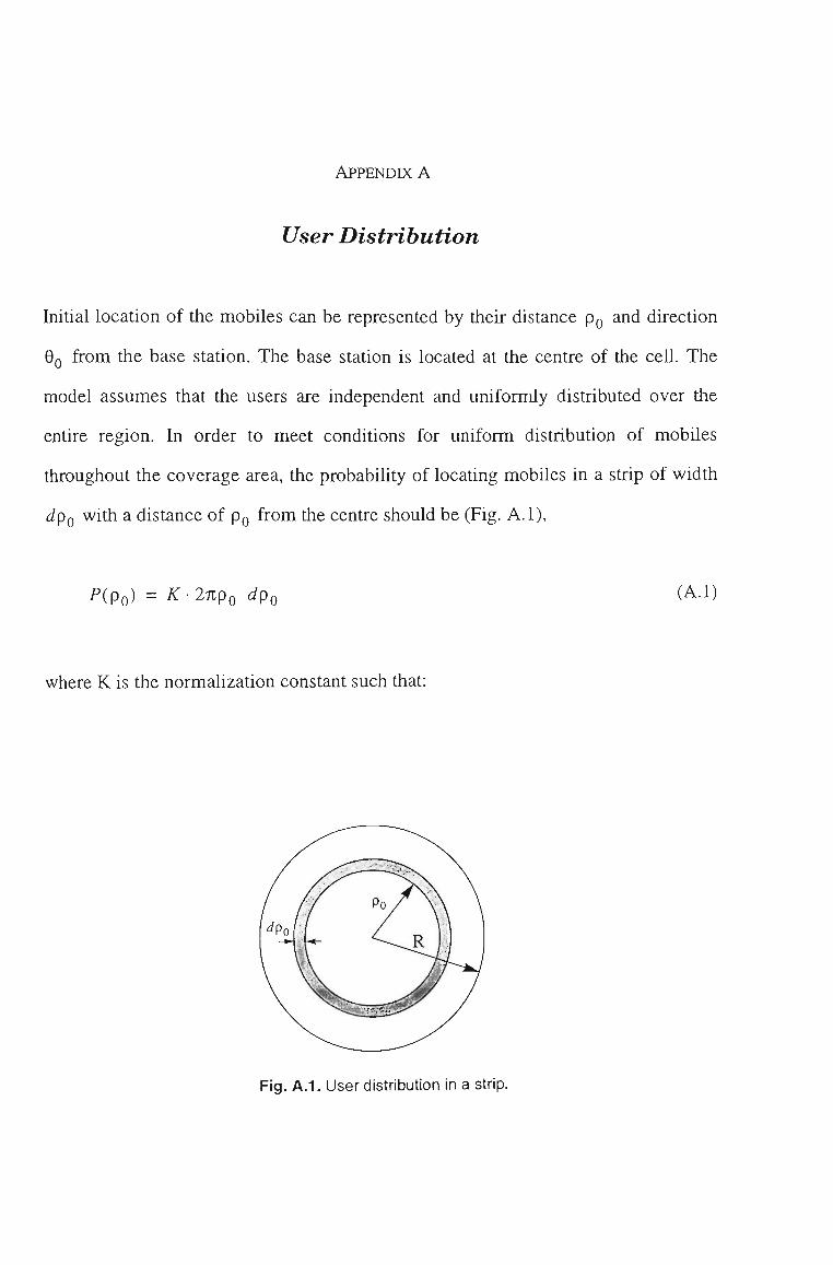
APPENDDC A
User Distribution
Initial location of the mobiles can be represented by their distance pg and direction
OQ from the base station. The base station is located at the centre of the ceU. The
model assumes that the users are independent and uniformly distributed over the
entire region. In order to meet conditions for uniform distribution of mobiles
throughout the coverage area, the probabihty of locating mobiles in a strip of width
dpo with a distance of PQ from the centre should be (Fig. A.l),
P(Po) = K-2npQ dpQ (A.1)
where K is the normalization constant such that:
Fig. A . l . User distribution in a strip.
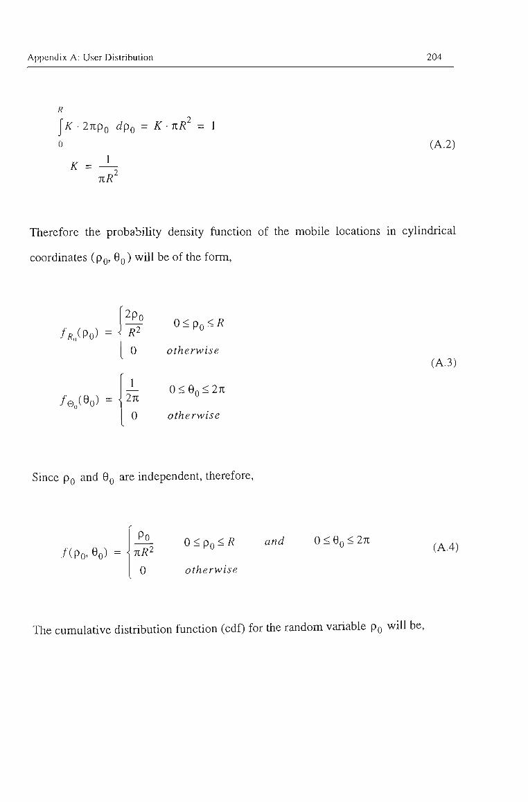
Appendix A: User Distribution 204
j /^-27lpo dpQ = KKR^ = 1
0
1 (A.2)
K = nR
Therefore the probabihty density function of the mobtie locations in cyhndrical
coordinates (pg, OQ ) wtil be of the form.
/RSPO)
2po
0 otherwise
— 0 < On < 27C
0 otherwise
(A.3)
Since pg and OQ are mdependent, therefore.
/(Po'^o) = 0
0 < P o ^ ^ and 0<QQ<2K
otherwise
(A.4)
The cumulative distribution function (cdf) for the random variable pg wiU be.
Appendix A: User Distribution 205
PRSPO) = j!l//?„(Po)^P( o2 (A.5) Po /?2
Using the probability integral transformation theorem, random numbers RQ with the
cdf of Fj^ (PQ) can be generated by a sequence of uniformly distributed numbers, U,
in the range of [0, 1 ] by,
Rr, = R4U (A.6)
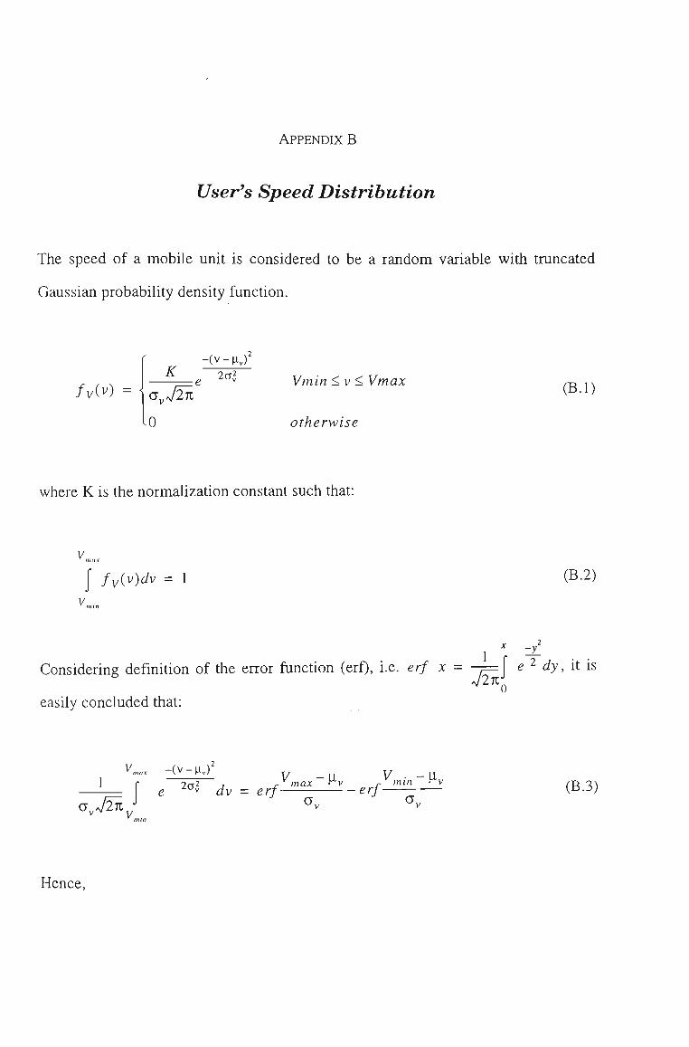
APPENDIX B
User's Speed Distribution
The speed of a mobile unit is considered to be a random variable with tmncated
Gaussian probability density function.
/v(v) e "
a^j2n
0
Vmin < V < Vmax
otherwise
(B.l)
where K is the normalization constant such that:
j fy{v)dV = I (B.2)
-y
Considering definition of the error function (erf), i.e. erf x = -=^ e ^ dy, it
easily concluded that:
is
Vn,ax -(V-PJ
0,7271,
y c T ' 7 r^ max ^v j . ^ min M-v
e °v dy = erf erf 2oi (B.3)
Hence,
Appendix B: User's Speed Distribution 207
K 1
J- max r^v r min r^v
erf erf
(B.4)
APPENDIX C
Minimum Value of Two Random Variables
If
2 = miniX, Y), ( Q 1 )
then.
Fz(z) = Fx(z) + FY(z)-F^{z)Fy{z) (C.2)
Proof:
The random variable Z is so defined that its value Z{Q for a given C, equals the
minimum of the two numbers X{C,),Y{1,). For a given z, the region D^ of the xy
plane such that,
min{x, y)<z that is x<z or y<z (C.3)
is shown in Fig. C.l. Hence, to find ^^(z), it suffices to determine the mass in D^.
This mass equals the mass F;^(z) in the half plane x<z plus the mass Fy(z) in the
half plane y<z minus the mass F^yiz, z) in the region x<z and y<z.
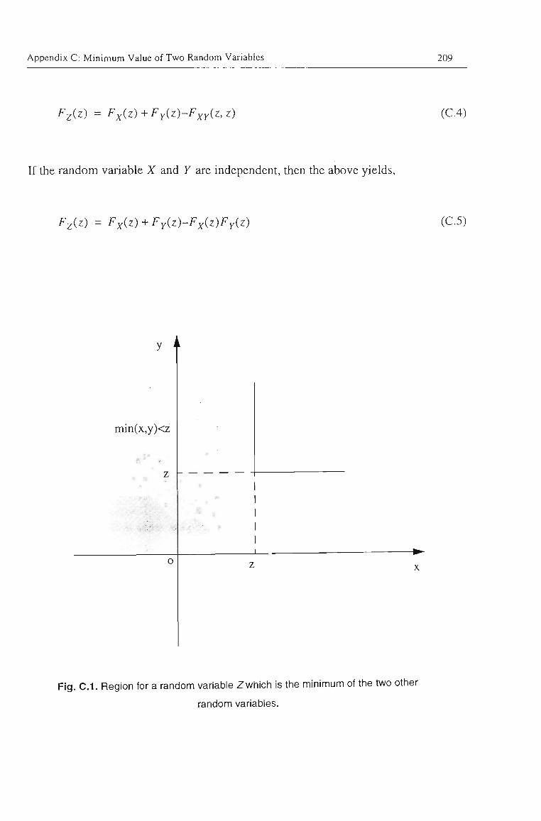
Appendix C: Minimum Value of Two Random Variables 209
F^{z) = F^{Z) + FY{Z)-F^Y(Z,Z) (C.4)
If the random variable X and Y are independent, then the above yields.
Fz(z) = F^{z) + FY(z)-F^{z)Fyiz) (C.5)
min(x,y)<z
o
Fig. C.I. Region for a random variable Zwhich is the minimum of the two other
random variables.
APPENDIX D
Expected Value of a Distribution
The average value of a random variable T^^ can be expressed directly in terms of its
distribution F-p (t). Since the channel holding time is limited in the range •' ch
0 < r ./, < Q then.
F^JO) = 0
F^Jt,) = 1
The average value of T^^ can be expressed in term of its density by.
Integrating (D.2) by parts, we obtain.
(D.l)
E[T^,] = \tfrjt)dt (D.2)
\tffJt)dt=tFrJt)\';-\FrJt)dt (D.3) 0 0
= to-\FTjt)dt
Hence, from (D.2) and (D.3), we obtain,
Appendix D: Expected Value of a Distribution
^[^c/J = ^0-tFTjt)dt (D.4)
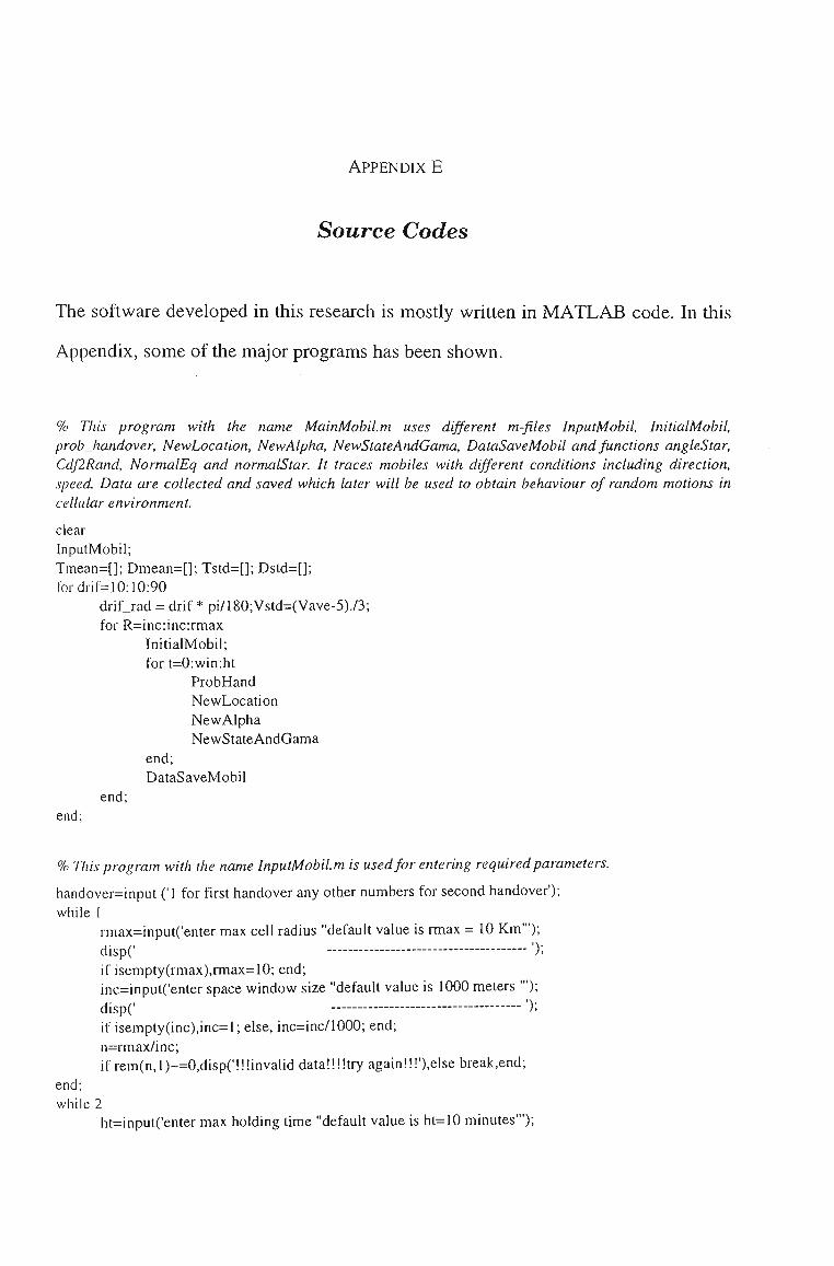
APPENDIX E
Source Codes
The software developed in this research is mostly written in MATLAB code. In this
Appendix, some of the major programs has been shown.
% This program with the name MainMobil.m uses different m-files InputMobil, InitialMobil, probjhandover, NewLocation, New Alpha, NewStateAndGama, DataSaveMobil and functions angleStar, CdflRand, NormalEq and normalStar. It traces mobiles with different conditions including direction, speed. Data are collected and saved which later will be used to obtain behaviour of random motions in cellular environment.
clear InputMobil; Tmean=[]; Dmean=[]; Tstd=[]; Dstd=[]; for drif=10:10:90
drif_rad ^ drif * pi/180;Vstd=(Vave-5)./3; for R=inc:inc:rmax
InitialMobil; for t=0:win:ht
ProbHand NewLocation NewAlpha NewStateAndGama
end; DataSaveMobil
end; end;
% This program with the name InputMobil.m is used for entering required parameters.
handover=input ('1 for first handover any other numbers for second handover'); while 1
rmax=input('enter max cell radius "default value is rmax - 10 Km'"); dispc '); if isempty(rmax),rmax=10; end; inc=input('enter space window size "default value is 1000 meters '"); dispC '); if isempty(inc),inc=l; else, inc=inc/1000; end; n=rmax/inc; if rem(n,l)~=0,disp('!!!invalid dataililtry again!!r),else break,end;
end; while 2
ht=input('enter max holding time "default value is ht=10 minutes'");
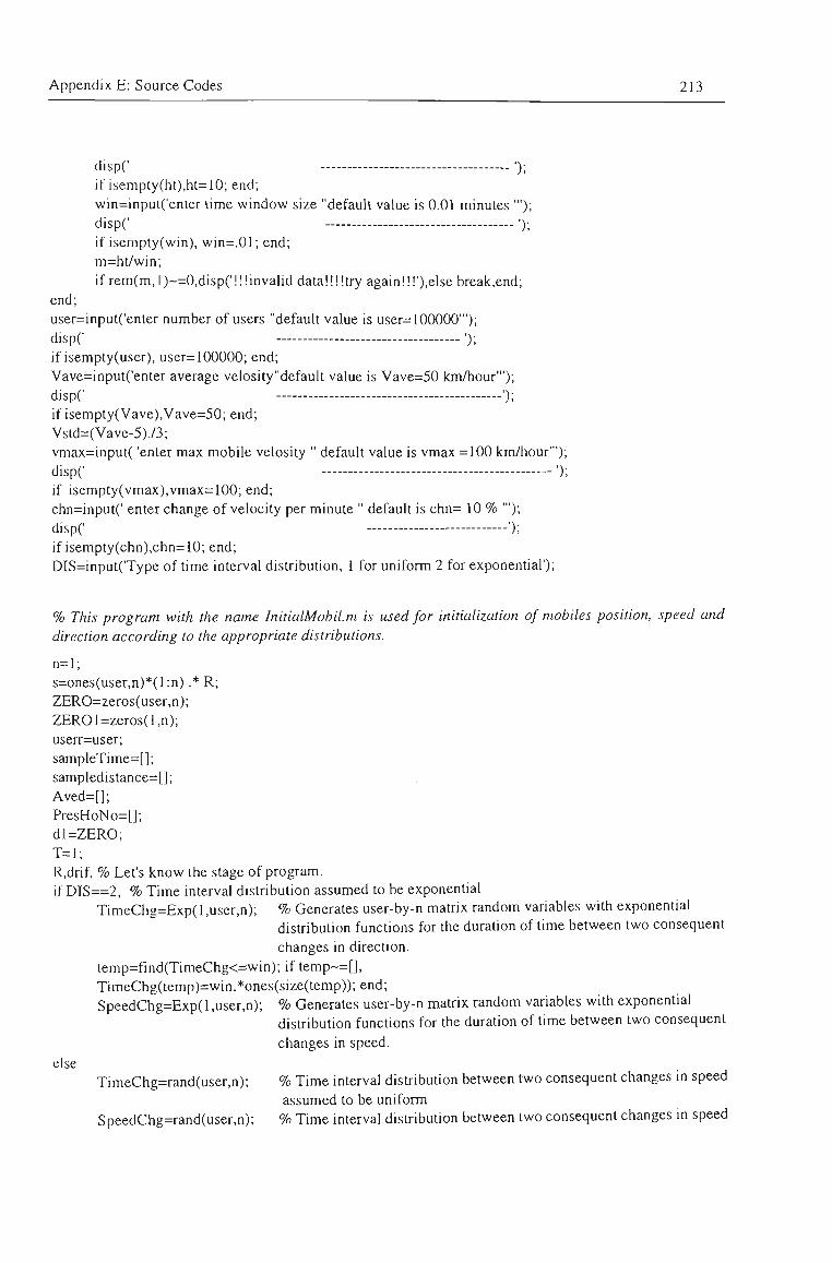
Appendix E: Source Codes 213
dispC '); if isempty(ht),ht=10; end; win=inpul('enter time window size "default value is 0.01 minutes "'); dispC '); if isempty(win), win=.01; end; m=ht/win; if rem(m,l)~=0,disp('!!!invalid data!!!!try again!!!'),else break,end;
end; user=input('enter number of users "default value is user= 100000'"); dispC •); if isempty(user), user=100000; end; Vave=input('enter average velosity"default value is Vave=50 km/hour'"); dispC •); if isempty(Vave),Vave=50; end; Vstd=(Vave-5)./3; vmax=input( 'enter max mobile velosity " default value is vmax =100 km/hour'"); dispC '); if isempty(vmax),vmax=100; end; chn=input(' enter change of velocity per minute " default is chn= 10 % '"); dispC '); if isempty(chn),chn=10; end; DIS=input('Type of time interval distribution, 1 for uniform 2 for exponential');
% This program with the name InitialMobil. m is used for initialization of mobiles position, speed and direction according to the appropriate distributions.
n=l; s=ones(user,n)*(l:n) .* R; ZERO=zeros(user,n); ZERO l=zeros( 1 ,n); userr=user; sampleTime=[]; sampledistance=[]; Aved=[]; PresHoNo=[]; dl=ZERO; T=l; R,drif, % Let's know the stage of program. if DIS==2, % Time interval distribution assumed to be exponential
TimeChg=Exp( 1 ,user,n); % Generates user-by-n matrix random variables with exponential distribution functions for the duration of time between two consequent changes in direction.
lemp=fmd(TimeChg<=win); if temp~=[], TimeChg(temp)=win.*ones(size(temp)); end; SpeedChg=Exp( 1 ,user,n); % Generates user-by-n matrix random variables with exponential
distribution functions for the duration of time between two consequent changes in speed,
else TimeChg=rand(user,n); % Time interval distribution between two consequent changes in speed
assumed to be uniform SpeedChg=rand(user,n); % Time interval distribution between two consequent changes m speed
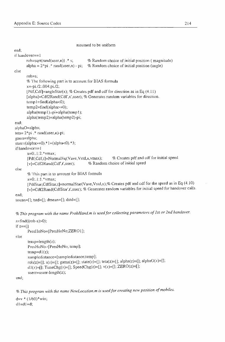
Appendix E: Source Codes 214
assumed to be uniform end; if handover==l
roh=sqrt(rand(user,n)) .* s; % Random choice of initial position ( magnitude) alpha = 2*pi .* rand(user,n) - pi; % Random choice of initial position (angle)
else roh=s; % The following part is to account for BIAS formula x=-pi./2:.004:pi./2; [Pdf,Cdf]=angleStar(x); % Creates pdf and cdf for direction as in Eq (4.11) [alpha]=Cdf2Rand(Cdf ,x',user); % Generates random variables for direction. temp 1=fmd(alpha<0); temp2=fmd(alpha>=0); alpha(temp 1 )=pi-i-alpha(temp 1); alpha(temp2)=alpha(temp2)-pi;
end; alphaO=alpha; teta= 2*pi .* rand(user,n)-pi; gama=alpha; state=(alpha>=0).*l+(alpha<0).*3; if hando ver== 1
x=0:.l:2.*vmax; [Pdf,Cdf,t]=NormalEq(Vave,Vstd,x,vmax); % Creates pdf and cdf for initial speed [v]=Cdf2Rand(Cdf ,t',user); % Random choice of initial speed
else % This part is to account for BIAS formula x=0:. 1:1.* vmax; [PdfStar,CdfStar,t]=normalStar(Vave,Vstd,x);% Creates pdf and cdf for the speed as in Eq (4.10) [v]=Cdf2Rand(CdfStar',t',user); % Generates random variables for initial speed for handover calls,
end; tmean=[]; tstd=[]; dmean=[]; dstd=[];
% This program with the name ProbHand.m is used for collecting parameters of 1st or 2nd handover.
z=fmd((roh-s)>0); ifz==[]
PresHoNo=[PresHoNo;ZERO 1 ]; else
temp=length(z); PresHoNo=[PresHoNo; temp]; temp=dl(z); sampledistance=[sampledistance;temp]; roh(z)=[]; s(z)=[]; gama(z)=[]; state(z)=[]; teta(z)=[]; alpha(z)=[]; alphaO(z)=[]; dl(z)=[]; TimeChg(z)=[]; SpeedChg(z)=[]; v(z)=[]; ZERO(z)=[]; usen-=userr-length(z);
end;
% This program with the name NewLocation.m is used for creating new position of mobiles.
d=v*(l/60)*win; dl=:dl+d;
Appendix E: Source Codes 215
rohN=sqrt ( roh .^1 + d.^2 + 2 * ((roh .* d).*cos(gama))); beta=abs(real(acos((rohN.^2-i-d.'^2-roh.^2)./(2*(rohN.*d))))); roh=rohN; BetaSign=((state==2)+(state==3))-((state== 1 )-t-(state==4)); teta=teta-l-gama-l-beta.*BetaSign; temp=find(teta> pi); if temp~=[], teta(temp)=teta(temp)-2*pi; end; temp=find(teta<-pi); if temp~=:[], teta(temp)=teta(temp)-l-2*pi;end;
% This program with the name NewAlpha.m is used for creating new position, velocity and direction for active mobiles.
aIpha=ZERO; temp=find(TimeChg<t+win & TimeChg>=t); if temp~=[]
ifDIS==2 TimeChg(temp)=Exp( 1 ,length(temp), 1 )+t+win;
else TimeChg(temp)=TimeChg(temp)+ones(size(temp));
end; alpha(temp)=2.*drif_rad .* rand(size(temp))-drif_rad; alphaOO=alphaO(temp)+alpha(temp); temp2=fi nd(alphaOO>pi); if temp2~=[], alphaOO(temp2)=alphaOO(temp2)-2*pir end; temp2=find(alphaOO<-pi); if temp2~=[], alphaOO(temp2)=alphaOO(temp2)+2*pi; end; alphatemp=alpha(temp); ph=pi./2; A= alphaO(temp)>0 & alphaO(temp)<ph & alpha(temp)>0 & alphaOO> ph; B= alphaO(temp)>ph & alphaO(temp)<pi & alpha(temp)<0 & alphaOO< ph; C= alphaO(temp)>-ph & alphaO(temp)<0 & alpha(temp)<0 & alphaOO<-ph; D= alphaO(temp)>-pi & alphaO(temp)<-ph & alpha(temp)>0 & alphaOO>-ph; E^A+B+C+D; if find(E>l)~=[],disp('error') ;end; templ=find(E==l); alphatemp(temp 1 )=zeros(size(temp 1)); alpha(temp)=alphatemp; alphaO(temp)=alphaO(temp)+alpha(temp); TimeChgtemp=TimeChg(temp); TimeChgtemp(templ)=(t+win).*ones(size(templ)); TimeChg(temp)=TimeChgtemp;
end; temp=find(SpeedChg<t-l-win & SpeedChg>=0; Speed_CHG=(2.*chn/100).* rand(userr,n) - chn/100; if temp~=[]
v(temp)=Speed_CHG(temp).*v(temp)+v(temp); if DIS==2
SpeedChg(temp)=Exp(l,length(temp),l)+t+win; else
SpeedChg(temp)=SpeedChg(temp)+ones(size(temp));
Appendix E: Source Codes 216
end; end; vl=find(v>vmax); if vl~=[], v(vl)=vmax.*ones(size(vl)); end; v2=find(v<=0); if v2-=[], v(v2)=0.0001.*ones(size(v2)); end;
% This program with the name NewStateAndGama.m is used for creating new state and angle gamma of mobiles.
state01d=state; region2=alpha< (-beta) I alpha> (pi-beta); region I=alpha>=(-beta) & alpha<=(pi-beta); region4=alpha> (beta) I alpha< (beta-pi); region3=alpha<=(beta) & alpha>=(beta-pi); if regionl==[], regionl=ZERO; end; if region2==[], region2=ZERO; end; if region3==[], region3=ZERO; end; if region4==[], region4=ZERO; end state= ((stateOld==l)-H(state01d==4)).*(regionl+region2.*2)+...
((state01d==2)+(state01d==3)).*(region3.*3+region4.*4); betaSign=(state==l)+(state==2)-(state==3)-(state==4); gama=alpha+beta.*betaSign;
% This program with the name DataSaveMobil.m is used for saving data.
Dmean=mean(sampledistance); Dstd=std(sampledistance); RR=R.*1000; p 1=num2str(handover); p2=num2str(Vave); p3=num2str(drif); p4=num2str(R); filename=['~/MATLAB/mobility/data/H' pi 'V p2 'drif p3 'R' p4]; eval(['save' filename ' PresHoNo drif R ht win user Vave handover Dmean Dstd;']);
% This function generates I-by-J matrix random variables with exponential distribution functions.
function [B]=Exp(A,I,J) B= - A.*log(rand(I,J));
% This function generates pdf and cdf for direction as in Eq (4.11)
function [Pdf,Cdf]=angleStar(x); Pdf=0.5.*cos(x); Cdf=.5+.5.*sin(x);
% This function generates random variables for different distribution functions.
function [RandNum]=Cdf2Rand(Cdf,t,No); CdfSh=Cdf( 1 :(length(Cdf)-1)); lemp=Cdf(2:length(CdO)-CdfSh; temp 1 =find(temp==0);
Appendix E: Source Codes 217
if templ~=[], Cdf(templ)=[]; t(templ)=[]; end; UU=min(Cdf)+(max(Cdf)-min(Cdf)).*rand(l,No); RandNum=::interpl(Cdf,t,UU);
% This function creates truncated normal distributions.
function [Pdf,Cdf,t]=NormalEq(Mu,Sigma,x,vmax); A=(2.*pi).^0.5; vmin=0; B=(vmax-Mu)./Sigma; BB=0.5.*erf(B./2.'^0.5); C=(vmin-Mu)./Sigma; CC=0.5.*erf(C./2.'^0.5); K=l./(BB-CC); t=vmin:.01 :vmax; Pdf=(K./(Sigma.*A)).*exp(-(t-Mu).'^2/(2.*Sigma.^2)); X=(t-Mu)./Sigma; Cdf = 0.5 + 0.5 .* erf(X ./ (2 . 0.5));
% This function creates pdf and cdf for Eq (4.10).
function [PdfStar,CdfStar,t]=normalStar(Mu,Sigma,x); vmax=100; [Pdf ,Cdf, t]=NormalEq (Mu, S igma, x, vmax); PdfStar=(t.*Pdt)./Mu; [CdfStar]=Pdf2Cdf(PdfStar,t);
% This function calculates pdf and cdf as shown in Eqs (4.5), (4.6), (4.8) and (4.9).
function [pdfHol,pdfHo2,cdfHol,cdfHo2,t]=RapHo(win, ht, vmax, rmax) t=win:win:ht; vmax l=vmax./60; R=rmax.*0.91; Limit=(2.*R)./vmaxl; temp I =find(t>=Limit); temp2=find(t<Limit); a=(2./pi).*asin((vmax 1 .*t(temp2))./(2.*R)); b=(4./(3.*pi)).*tan((l./2).*asin((vmaxl.*t(temp2))./(2.*R))); c=(l./(3.*pi)).*sin(2.*asin((vmaxl.*t(temp2))./(2.*R))); e=(8.*R)./(3.*pi.*vmaxl.*t(templ)); 1=1-e; g=l-1.5.*e; cdfHol=a-b+c; cdfflol=[cdtHol,f]; cdfHo2=a-b.*3./2; cdfHo2=[cdfHo2,g]; aa=(8.*R)./(3.*pi.*vmaxl.*t(temp2).*t(temp2)); bb=((vmaxl.*t(temp2))./(2.*R)).'^2; cc=l-(l-bb).^1.5; dd=(8.*R)./(3.*pi.*vmaxl.*t(templ).*t(templ)); ee=l-(l-bb).'^0.5;
Appendix E: Source Codes 218
ddd=1.5.*dd; pdfHol=aa.*cc; pdfHol=[pdlHol,dd]; pdfHo2=(aa.*1.5).*ee; pdlHo2=[pdfHo2,ddd]; pdlHol=[0,pdfHol]; pdtHo2=[0,pdtHo2]; cdfHoI=[0,cdfHol]; cdtHo2=[0,cdfHo2]; t=0:win:ht;
% This program with the name RapNewCall.m plots new call residance time probability distributin for two different case of simulation andEq (4.6) with the same mobility parameters. It is shown in Fig. 4.5.
clear;
load ~/MATLAB/mobility/data/RAP/HlV100Rl_10.mat % data file from simulation t=0:win:ht; PDFl=PresHoNo./(user.*win); CDFl=cumsum(PresHoNo./user); % cdf as obtained from simulation for i-inc;inc;rmax
[pdfHol,pdfHo2,cdfHol,cdfHo2, tt]=RapHo(win.*10, ht, vmax, r); CDF_H01=[CDF_H01,cdfHol']; % cdf as obtained from equation (4.8)
end clg;figure(l) plot(t,CDFl,'-'); % Plots simulation results hold on; grid on plot(tt,CDF_H01); % Plots analytical results xlabel('New Call Cell Residence Time (minute)') ylabel('Probability') hold off
% This program with the name RapHoCallm plots harwver call residence time probability distribution using two different cases of simulation and Eq (4.9) with the same mobility parameters. The figure is shown in Fig. 4.5.
clear load ~/MATLAB/mobility/data/RAP/H2V100Rl_10.mat; % data file from simulation t=0:win:ht; PDFl=PresHoNo./(user.*win); CDFl=cumsum(PresHoNo./user); for r=inc:inc:rmax
[pdfHol,pdfHo2,cdfHol,cdfHo2, tt]=RapHo(win.*10, ht, vmax, r); CDF_H02=[CDF_H02,cdfHo2'];% cdf as obtained from equation 4.9
end clg; figure(l) plot(t,CDFl,'- ');% Plots simulation results hold on; grid on; plot(tt,CDF_H02); % Plots analytical results xlabel('Handover Call Cell Residence Time (minute)') ylabel('Probability') hold off
Appendix E: Source Codes 219
% This program with the name FitCdfGamma.m fits the obtained data for handover probability to a generalised gamma distribution
clear Al=[]; ERRORm=inf;Vave=50;drif=0; alpha=[];beta=[]; handover=input('enter 1 for new calls and 2 for handover calls'); alphaL=input('enter lower limit of alpha parameter') alphaU=input('enter upper limit of alpha parameter') alphal=input('enter increment for the alpha parameter') betaL=input('enter lower limit of beta parameter') betaU=input('enter upper limit of beta parameter') betal=input('enter increment for the beta parameter') pL=input('enter lower limit of p parameter') pU=input('enter upper limit of p parameter') pl=input('enter increment for the p parameter') forR=10:10:100
RR=R./10; p I=num2str(handover); p2=num2str(Vave); p3=num2str(drif); p4=num2str(R); filename=['~/MATLAB/mobility/data/H' pi 'V p2 'drif p3 'R' p4]; eval(['load' filename]); t=(0:win:ht)'; [Pdfl=Data2Pdf(PresHoNo,t); [Cdfl=Pdf2Cdf(Pdf,t); ERRORm=inf; for p=pL:pI:pU
for alpha=alphaL:alphaI:alphaU for beta=betaL:betaI:betaU
[PDF,CDF]=GammaEq(alpha,beta,p,t); Error=max(abs(CDF-Cdf)); ifERRORm>Error
alphaO=alpha; betaO=beta; pO=p; ERRORm=Error;
end; end;
end; end; betaR=betaO./R; A= [R alphaO, betaR, pO, ERRORm]; A1=[A1,A]
end;
% This function generates pdf for any input data. In our case input data is 'PresHoNo' which describes statistics for number of tiandovers.
function [Pdl]=Data2Pdf(Data,t); Pdf=Data./sum(Data); % rough estimation of Pdf PdfArea=trapz(t,PdO; Pdf=(Pdf/Pdf Area); % final result of Pdf
Appendix E: Source Codes 220
% This function converts pdf to cdf
function [Cdf|=Pdf2Cdf(Pdf t); if length(Pdf)~=length(t), error('error in Pdf2Cdf), end; if length(Pdf) > 200
win=t(2)-t(l); Cdf=cumsum(Pdf(l:length(Pdf))).*win;
else Cdf=0; Bins_Area=0; fori=l:length(Pdf)-l
BinArea=trapz([t(i), t(i+l)],[Pdf(i),Pdf(i+l)]); Bins_Area=BinArea-i-Bins_Area; Cdf=[Cdf;Bins_Area];
end; end;
% This function generates pdf and cdf for the generalized gamma distribution.
function [Pdf,Cdf]=GammaEq(alpha,beta,p,t); a=exp(-(t./beta).''^p); b=t.'^(p.*alpha-l); c=beta.^(p.*alpha); d=gamma(alpha); Pdf=(p.*b.*a)./(c.*d); [Cdf]=Pdf2Cdf(Pdf,t);
% This program with the name BestRDrift.m chooses cells with different drifts with the best fit with a reference cell.
clear Vave=50; drift =0; handover=input('enter 1 for new calls and 2 for handover calls'); for drifdrif=10:10:90
forRR=10:10:100 p l=num2str(handover); p2=num2str(Vave); p3=num2str(drifdrif); p4=num2str(RR); filename=['~/MATLAB/mobility/data/H' pi 'V p2 'drif p3 'R' p4]; eval(['load' filename]); RX=R; t=(0:win:ht)'; [Pdf]=Data2Pdf(PresHoNo,t); [Cdf|=Pdf2Cdf(Pdf,t); ERRORm=inf; forRl=RR:l:2.*RR
p3=num2str(drif 1); p4=num2str(Rl); filename=['-/MATLAB/mobility/data/H' pi 'V p2 'drif p3 'R' p4]; eval(['load' filename]);
Appendix E: Source Codes 221
[PDF]=Data2Pdf(PresHoNo,t); [CDF]=Pdf2Cdf(PDF,t); Error=max(abs(CDF-Cdf)) clear PresHoNo; if ERRORm>Error, ERRORm=Error; Rm=Rl.*100; end;
end p3=num2str(drifdrif); p4=num2str(RX); filename=['-/MATLAB/mobility/data/Drift/H' pi 'V p2 'drif p3 'R' p4]; eval(['save' filename ' Rm ERRORm;']);
end; end;
% This program with the name BestRVel.m chooses cells with different speeds with the best fit with a reference cell.
clear Vave 1=50; drif=0; handover=input('enter 1 for new calls and 2 for handover calls'); for VaveVave=10; 10:80
forRR=10:10:100 p l=num2str(handover); p2=num2str(VaveVave); p3=num2str(drif); p4=num2str(RR); filename=['~/MATLAB/mobility/data/H' pi 'V p2 'drif p3 'R' p4]); eval(['load' filename]); RX=R; t=(0:win:ht)'; [Pdfl=Data2Pdf(PresHoNo,t); [Cdf]=Pdf2Cdf(Pdf,t); ERRORm=inf; forRl=l:l:l.*RR
p2=num2str(Vave 1); p4=num2str(Rl); filename=['~/MATLAB/mobility/data/H' pi 'V p2 'drif p3 'R' p4]); eval(['load' filename]); [PDF]=Data2Pdf(PresHoNo,t); [CDF]=Pdf2Cdf(PDF,t); Error=max(abs(CDF-Cdf)); clear PresHoNo; if ERRORm>Error, ERRORm=Error; Rm=Rl.*100; end;
end; p2=num2str(VaveVave); p4=num2str(RX); filename=['~/MATLAB/mobility/dataA^elocity/H' pi 'V p2 'drif p3 'R' p4]; eval(['save' filename' Rm ERRORm;']);
end; end;
Appendix E: Source Codes 222
% This program with the name diff_gamma.m plots Fig. 4.7 which shows examples of different generalized gamma density functions.
clear; win=.5; ht=30; t=0:win:ht; figure(l) alpha=l; beta=6; p=l; [pdf,cdfl=GammaEq(alpha,beta,p,t); % Exponential distribution plot(t,pdf,'m-') hold on alpha=3; beta=4; p=l; [pdf,cdf]=GammaEq(alpha,beta,p,t); % Gamma distribution plot(t,pdf,'-') alpha=l; beta=25; p=12; [pdf cdf]=GammaEq(alpha,beta,p,t); % Weibuil distribution pIot(t,pdf,'r:','LineWidth', 1) alpha= 1 ;beta=5.*2.'^(l/2);p=2; [pdf cdf]=GammaEq(alpha,beta,p,t); % Rayleigh distribution plot(t,pdf'g-.') 11=10; alpha=n./2; beta=2; p=l; [pdf cdf]=GammaEq(alpha,beta,p,t); % chi square distribution plot(t,pdf'w-') ylabel('Probability density') hold off
% This programwith the name Pdf_GamaData_HOI .m plots new or hanover call residence time pdf using two different cases of simulation and generalized gamma distribution. The figure is shown in Fig. 4.8.
clear; handover=input('enter 1 for new calls and 2 for handover calls'); Vave=input('enter intial average velosity'); drif=input('enter the amount of drift'); R=input('enter the amount of cell size in Km'); R=R.*10; eval(['load ~/MATLAB/mobility/data/H' num2str(handover) 'V num2str(Vave) 'drif num2str(drif) 'R' nuin2str(R)]) t=(0:win;ht)'; [Pdi]=Data2Pdf(PresHoNo,t); % Pdf according to simulation data [Cdl]=Pdf2Cdf(Pdf t); % Pdf according to simulation data if handover= 1, alpha=.62; beta=1.84.*R; p=1.88; end; if handovei-2, alpha=2.31; beta=1.22.*R; p=1.72; end; [Pdf l,Cdfl]=GammaEq(alpha, beta, p, t); % Pdf according to equivalent gamma distribution. figure plot(t( 1:10:length(t)),Pdf(l:10:length(Pdf)),'g'); temp=max(Pdf); axis([0,25,0,.16]) hold on plot(t,Pdf 1 ,'-','LineWidth',2); grid on;
Appendix E: Source Codes 223
% This program with the name Cdf_GamaData_HOI.m plots new or hanover call residence time pdf using two different cases of simulation and generalized gamma distribution. The figure is shown in Fig. 4.9.
clear; handover=input('enter 1 for new calls and 2 for handover calls'); Vave=input('enter intial average velosity'); drif=input('enter the amount of drift'); for R= 10:10:100
p l=num2str(handover); p2=:num2str(Vave); p3=num2str(drif); p4=num2str(R); filename=['~/MATLAB/mobility/data/H' pi 'V p2 'drif p3 'R' p4]; eval(['load' filename]); t=(0:win:ht)'; [Pdf]=Data2Pdf(PresHoNo,t); [Cdf]=Pdf2Cdf(Pdf,t); if handover=l, alpha=.62; beta=1.84.*R; p=1.88; end; if handover=2, alpha=2.31; beta=1.22.*R; p=1.72; end; [Pdfl,Cdfl]=GammaEq(alpha,beta,p,t); plot(t,Cdf); hold on; plot(t,Cdfl,'r-');
end; axis([0,20,0,l]); t=0:win:ht; grid on; if handovei-1, xlabel('New Call Cell Residence Time (minute)'); end; if handover=2, xlabel('Handover Call Cell Residence Time (minute)'); end; ylabel('Probability'); hold off;
% This program with the name MEAN.m compares the mean cell residence time for the new and the Imndover calls with different calculation methods as shown in Table 4.3
V=50; drif=0; handover=input('enter 1 for new calls and 2 for handover calls'); for R=l: 1:10
if handover=l, alpha=.62; beta=1.84.*R; p=1.88; end; if handover=2, alpha=2.31; beta=1.22.*R; p=1.72; end; pl=num2str(handover); p2=num2str(Vave); p3=num2str(drif); p4=num2str(R); filename=['-/MATLAB/mobility/data/H' pi 'V p2 'drif p3 'R' p4]; eval(['load' filename]); t=(0:win:ht)'; [Pdf]=Data2Pdf(PresHoNo,t); [mu]=Pdf2mean(Pdf t); % mean value according to the Eqs (4.23) and (4.24)
Appendix E: Source Codes 224
% This program with the name EqRdrift.m compares simulation results with the empirical formula as shown in Fig. 4.11.
Vave=:50;r=l:l:10;j=0; handover=input('enter 1 for new calls and 2 for handover calls'); for drif= 10:10:90
Extra=[]; Excess=[]; forR=l:l:10
p 1=num2str(handover); p2=num2str( Va ve); p3=num2str(drif); p4=num2str(R.*10); filename=['~/MATLAB/mobility/data/Drift/H' pi 'V p2 'drif p3 'R' p4]; eval(['load' filename]); excess=Rm-R; % Excess cell radius for different values of drift by simulation extra=0.0038.*drif *R; % Excess cell radius by empirical equation (4.28). Excess=[Excess, excess]; Extra=[Extra, extra];
end;
subplot(3,3,j), plot(r, Extra, 'w.', r. Excess,'g') axis([ 1,10,0,3]) grid on; hold on; ylabel('Excess Radius (Km)'); xlabeK'Cell Radius (Km)');
end; hold off
% This program with the name EqRvelocityHOl.m compares simulation results with the empirical formula as shown in Fig. 4.12.
clear drif=0;r=l:l:10; handover=input('enter 1 for new calls and 2 for handover calls'); for Vave=10:10:70
Extra=[]; Excess=[]; for R=l: 1:10
pl=num2str(handover); p2=num2str(Vave); p3=num2str(drif); p4=num2str(R.*10); filename=['~/MATLAB/mobility/data/Drift/H' pi 'V p2 'drif p3 'R' p4]; eval(['load' filename]); excess=Rm-R; % Excess cell radius for different speeds by simulation extra=((50.A'ave)-l).*R; % Excess cell radius by empirical equation (4.31). Excess=[Excess, excess]; Extra=[Extra, extra];
end; plot(r. Extra, 'w.', r, Excess,'g') grid on; hold on;
Appendix E: Source Codes 225
ylabel('Excess Radius (Km)'); xlabeK'Cell Radius (Km)'); axis([ 1,10,-3,10]) ylabel('Excess Radius (Km)') xlabeK'Cell Radius (Km)') end;
hold off
% This function calculates the mean value for a given pdf
function [mu]=Pdf2mean(Pdf,t) temp=t.*Pdf; mu=trapz(t,temp);
% This program with the name ave_ho_Pfh.m calculates and plots (as in Fig. 4.14) average number of
handovers experienced by a random call for different probabilities of handover failures.
clear Vave=50; drif=0; AveCallHoldTime=2; win=.01; ht=100; t=0:win:ht;R=l:l:10;Ri=l:l./4:10; forPfli=[0,.l,.2,.5]
AveH_G=[]; HH2=[]; HHg=[]; HH2g=[]; mu_InvTh=[]; for RR=1:1:10
handover=l; alpha=.62; beta=1.84.*RR; p=1.88; [Pdfn,Cdfn]=GammaEq(alpha,beta,p,t); handover=2; alpha=2.31; beta=1.22.*RR; p=1.72; [Pdfh,Cdfli]=GammaEq(alpha,beta,p,t); [Pn]=Pn_OR_Ph(Pdfn,AveCallHoldTime,t); [Ph]=Pn_OR_Ph(Pdfh,AveCallHoldTime,t); [H]=AveHoNo(Pn,Ph,Pfh); AveH_G=[AveH_G;H]; % First method ifPfti==0
[mu_Thl]=Pdf2mean(Pdfh,t); HH=(AveCallHoldTime)./mu_Th 1; AveH_T=[AveH_T; HH]; % Second method using equation (4.47)
end end; AveH_Gi=interpl(R,AveH_G',Ri,'spline'); AveH_Ti=inteipl(R,AveH_T',Ri,'spline'); plot(Ri, AveH_Gi) hold on plot(Ri, AveH_Ti,'r-'); ylabeI('Average Number of Handovers per Call') xlabeK'Cell Radius, R (Km)') hold off
% This function calculates probability that a handover call or a new call will require at least another handover as in Eqs (4.41) and (4.42).
function [P]=Pn_OR_Ph(PdfAveCallHoldTime,t) mu_c= 1 ./AveCallHoldTime;
Appendix E: Source Codes 226
FUNCTION=Pdf *exp(-mu_c. *t); P=trapz(t,FUNCTION);
% This function calculates average number of handovers per call as in (4.38)
function [H]=AveHoNo(Pn,Ph,Pfh) temp=l-Pfti;
H=(Pn. *temp)./( 1-Ph. *temp);
% This program with the name Th_Tn_Tc_Tch.m calculates and plots (as in Fig. 4.17) different fiinctions for a cell size of 3 Km.
path(path,'/pgr/mahmood/_framemaker/figures/mobility'); path(path,'/pgr/mahmood/MATLAB/mobility/dataprocces/Functions'); path(path,'/pgr/mahmood/MATLAB/Distribution/Data2Dist'); path(path,'/pgr/mahmood/MATLAB/DistributionyEq2Dist'); win=.l;ht=100;inc=l;rmax=10; handover=l; Vave=50; drif=0; R=30;
eval(['load /pgr/mahmood/MATLAB/mobility/data/H' num2str(handover) 'V num2str(Vave) 'drif num2str(drif) 'R' num2str(R)]) t=(0:win:ht)'; [Pdf n]=Data2Pdf(PresHoNo.t); [Cdfn]=Pdf2Cdf(Pdfn,t); handover=2; R=30;
eval(['load /pgr/mahmood/MATLAB/mobility/data/H' num2str(handover) 'V num2str(Vave) 'drif num2str(drif) 'R' num2str(R)]) [Pdfh]=Data2Pdf(PresHoNo,t); [Cdfli]=Pdf2Cdf(Pdfli,t); AveTime=2; [PdfCall,CDFCaIl]=ExpEq(AveTime,t); [CDFch]=CdfCh(Pdfn,Cdfn,Pdfh,Cdfh,AveTime,t); [muCh]=Cdf2mean(CDFch,t); [Pdfchannel,CDFchannel]=ExpEq(muCh,t); [Pn]=Pn_OR_Ph(Pdfn,AveTime,t); [Ph]=Pn_OR_Ph(Pdfti,AveTime,t); Pfh=0; [H]=AveHoNo(Pn,Ph,Pfh);% Ave Ho No First method F_Tch=CDFCall+(l./(l+H)).*(l-CDFCall).*(Cdfn+H.*Cdfli); z=l;]0:!ength(t); ploKKz),Cdfn(z),'b-');hold on axis([0, 10,0,1]) ploKKz)>Cdfli(z),'r.','LineWidth',2) plot(Kz),CDFCall(z),'g-.') plot(t(z),CDFchanneI(z),'c') text(t(z),F_Tch(z),'*','clipping','on','HorizontalAlignment','right','VerticalAlignment','top','FontSize',7) axis([0,10,0,1]); ylabel('Probability') xlabeK'Time (minute)') hold off;
Appendix E: Source Codes 227
% This function calculates pdf and cdf of the exponential distribution by using the related relation
function [Pdf,Cdf|=ExpEq(AveTime,t); Pdf=( 1 ./AveTime).*exp(-t./AveTime); Cdf= 1 -exp(-t./AveTime);
% This function calculates call holding time distributions as in (4.53)
function [CDFch]=CdfCh(Pdfn,Cdfn,Pdfli,Cdfh,AveCallHoldTime,t) [Pn]=Pn_OR_Ph(Pdfn,AveCallHoldTime,t); [Ph]=Pn_OR_Ph(Pdfli,AveCallHoldTime,t); [PdfCall,CdfCall]=ExpEq(AveCallHoldTime,t); ratio=Pn./(1 -Ph); ratio=ones(length(Cdfh),l)*ratio; ratiol=l./(l-(-ratio); CDFch=CdfCall+ratiol.*(l-CdfCall).*(Cdfn+ratio.*Cdfli);
% This function calculates mean value from cdf
function [mu]=Cdf2mean(Cdf,t) CdfArea=trapz(t,Cdf); mu=t(length(Cdf))-CdfArea;
% This program with the name mu.m calculates and plots (as in Fig. 4.18) variation of the average channel holding time with different cell sizes
clear; Vave=50; drif=0; AveCallHoldTime=2; win=.01; ht=100; t=0:win:ht; Pfli=0; AveH_G=[]; HH2=[]; HHg=[]; HH2g=[]; mu=[]; for R=l: 1:10
handover=l; alpha=.62; beta=1.84.*R; p=1.88; [Pdfn,Cdfn]=GammaEq(alpha,beta,p,t); handover=2; lpha=2.31; beta=1.22.*R; p=1.72; [Pdfh,Cdfli]=GammaEq(alpha,beta,p,t); [CDFch]=CdfCh(Pdfn',Cdfn',Pdfti',Cdfh',AveCallHoldTime,t'); [muCh]=Cdf2mean(CDFch,t); [mu]=[mu; muCh];
end; niu=60.*mu; R=l:l:10;Ri=l:l./4:10; mui=interpl(R,mu,Ri,'spline'); plot(Ri,muCh3i)
% This program creates data required for the traffic analysis
clear cellsize=l;ch=50;ch_ho=0; ch_new=ch - ch_ho;attempt=.33; InitialTraffic; forch_ho=0:l:5
ch=50; ch_new=ch - ch_ho;
Appendix E: Source Codes 228
for cellsize=l:10 for attempt=.04:.002:.05 % minute per call
landa=l./(attempt.*60)% call per second LANDA=round(landa.*100),% for deleting point in data saving InitialTraffic; LOOPSteady=30000; fori=l:LOOPSteady
SteadyState end; savedataTraffic; % steady state data fori=l:LOOP
BodyTraffic end; savedataTraffic
end; end;
end;
% This program with the name InitialTrqffic.m is used for initialization of parameters required for traffic analysis
cells=49; ARR=2; % mean call holding time [min]; LOOP=10000; CDF_1_2 NewCall=zeros(l,cells); NewCallBlock=zeros(l,cells); HoCall=zeros(l,cells); HoCallBlock=zeros(l,cells); ChannelStatus=zeros(l,cells); NoCallSuccess=zeros( 1 ,cells); st=inf.*ones( 1 ,cells); sp=inf *ones(ch,cells); ho=inf *ones(ch,cells); old_ho=inf *ones(ch,cells); dropout=zeros(l,cells); sourceCell=inf.*ones(ch,cells); % attributes of calls in process st( 1 ,:)=Exp(attempt, 1,cells); % attempt = duration between two successive call [min] clock=min(min(st)); i=0; ii=0;
% This program with the name SteadyState.m is used for approaching to the steady state condition.
[a]=find(st==clock); ifa~=[],
if length(a)>l, a=min(a); end; if ChannelStatus(a)<ch_new
ChannelStatus(a)=ChannelStatus(a)+1; B=min(find(sp(:,a)==inf)); sp(B,a)=Exp(ARR,l,l)+clock; % CallTime=Exp(ARR,l,l); ho(B ,a)=Cdf2Rand(CDF 1 ,X, 1 )-Hclock; sourceCell(B,a)=a;
end;
Appendix E: Source Codes 229
st(a)=Exp(attempt, l,l)-f-clock; % start time of the future call end; [A,a]=find(sp==clock); ifA~=[],
if length(A)>l, A=min(A); a=min(a); end; sp(A,a)=inf; ho(A,a)=inf; ChannelStatus(a)=ChannelStatus(a)-l; sourceCell(A,a)=inf;
end; [A,a]=find(ho==clock); ifA~=[]
if length(A)>l, A=min(A); a=min(a); end; ho(A,a)=inf; ChannelStatus(a)=ChannelStatus(a)-l; CellN=CellNo(old_ho(A,a),a); old_ho(A,a)=inf; if ChannelStatus(CellN)<ch
ChannelStatus(CellN)=ChannelStatus(CellN)+l; B=min(find(sp(:,CellN)==inf)); % to find place of empty channel sp(B,CellN)=sp(A,a); ho(B,CellN)=Cdf2Rand(CDF2,X,l)+clock; old_ho(B,CellN)=a; % gives the number of previous cell sourceCell(B,CellN)=sourceCell(A,a);
end; sp(A,a)=inf; sourceCell(A,a)=inf;
end; clockl=min(min(st)); % start time of the future call clock2=min(min(sp)); % stop time of the current call clock3=min(min(ho)); % ho time of the current call clock=min([clockl, clock2, clock3]);
% This program with the name savedataTraffic.m is used for saving data
iii=ii+l; ch_hoJi_R_Att=[ch_ho ,ii, cellsize, LANDA ] seed=rand('seed'); % seed for generating next variable p 1 =num2str(cellsize); p2=num2str(LANDA); p3=num2str(ch); p4=num2str(ch_ho); filename=['~/MATLAB/traffic/data/R' pi 'E" p2 'C p3 'H' p4]; clear X PDFl CDFl PDF2 CDF2 eval(['save ' filename]); CDF_1_2
% This program with the name BodyTraffic.m generates: attributes of the current call
[a]=find(st==clock);
ifa~=[], if lensth(a)>l, a=min(a); end;
Appendix E: Source Codes 230
Ne wCal l(a)=NewCall(a)-l-1; if ChannelStatus(a)<ch_new
ChannelStatus(a)=ChannelStatus(a)-i-l; B=iTiin(find(sp(:,a)=inf)); sp(B,a)=Exp(ARR,l, l)+clock;% CallTime=Exp(ARR, 1,1); ho(B ,a)=Cdf2Rand(CDF 1 ,X, 1 )-hclock; sourceCell(B ,a)=a;
else Ne wCallBlock(a)= NewCallBlock(a)-i-1;
end; st(a)=Exp(attempt, 1,1 )-l-clock; % start time of the future call
end; [A,a]=find(sp==clock); ifA~=[],
if length(A)>l, A=min(A); a=min(a); end; sp(A,a)=inf; ho(A,a)=inf; ChannelStatus(a)=ChannelStatus(a)-l; sourceCell(A,a)=inf; NoCall S uccess(a)=NoCallSuccess(a)-l-1
end; [A,a]=find(ho==clock); if A~=[]
if length(A)>l, A=min(A); a=min(a); end; ho(A,a)=inf; ChannelStatus(a)=ChannelStatus(a)-l; CellN=CellNo(old_ho(A,a),a); HoCall(CellN)=HoCall(CellN)+1; old_ho(A,a)=inf; if Channels tatus(CellN)<ch
ChannelStatus(CellN)=ChannelStatus(CellN)-H 1; B=min(find(sp(:,CellN)==inf)); % to find place of empty channel sp(B,CellN)=sp(A,a); ho(B ,CellN)=Cdf2Rand(CDF2,X, 1 )-hclock; old_ho(B ,CellN)=a; % gives the number of previous cell sourceCell(B,CellN)=sourceCell(A,a);
else HoCallBlock(CellN)=HoCallBlock(CellN)+l; dropout(sourceCell(A,a))=dropout(sourceCell(A,a))+1;
end; sp(A,a)=inf; sourceCeU(A,a)=inf;
end; clock l=min(min(st)); % start time of the future call clock2=min(min(sp)); % stop time of the current call clock3=min(min(ho)); % ho time of the current call clock=inin([clockl, clock2, clock3]);
% This program with the name CDF_l_2.m creates pdf and cdf of the generalised Gamma distributions
X=(0:.01:100)';
Appendix E: Source Codes 231
alpha=0.62; beta=1.84.*cellsize; p=1.88; %handover=l; [PDFl,CDFl ]=GammaEq(alpha,b6ta,p,X); alpha=2.31; beta=1.22.*cellsize; p=1.72; %handover=2; [PDF2,CDF2]=GammaEq(alpha,beta,p,X);
% This function creates the cell number to which a handover call is arrived.
function [CellN]=CellNo(old,a) U=fix(l-K(7-l).*rand); while U==7, U=fix(l-(-(7-l).*rand); end; replace=['CellN=XX(U); while CellN=old, U=fix(l+(7-l).*rand); while U = 7 , U=fix(l+(7-l).*rand); end; CellN=XX(U); end;']; if a== 1, XX=[ 2 8 14 7 46 47]; eval(replace) elseifa==2, XX=[3 9 8 1 47 48]; eval(replace) elseif a== 3, XX=[ 4 10 9 2 48 49]; eval(replace) elseif a== 4, XX=[ 5 11 10 3 49 43]; eval(replace) elseif a== 5, XX=[ 6 12 11 4 43 44]; eval(replace) elseif a== 6, XX=[ 7 13 12 5 44 45]; eval(replace) elseif a== 7, XX=[ 1 14 13 6 45 46]; eval(replace) elseif a== 8, XX=[ 9 16 15 14 1 2]; eval(replace) elseif a== 9, XX=[10 17 16 8 2 3]; eval(replace) elseif a==10,XX=[ 11 18 17 9 3 4]; eval(replace) elseif a==ll, XX=[12 19 18 10 4 5]; eval(replace) elseif a==12, XX=[13 20 19 11 5 6]; eval(replace) elseif a==13, XX=[14 21 20 12 6 7]; eval(replace) elseifa==14, XX=[8 15 21 13 7 1]; eval(replace) elseifa==15, XX=[16 22 28 21 14 8]; eval(replace) elseifa==16, XX=[17 23 22 15 8 9]; eval(replace) elseif a==17, XX=[18 24 23 16 9 10]; eval(replace) elseif a==18, XX=[19 25 24 17 10 11] elseif a==19, XX=[20 26 25 18 11 12] elseif a==20, XX=[21 27 26 19 12 13] elseif a==21, XX=[15 28 27 20 13 14] elseif a==22, XX=[23 30 29 28 15 16] elseif a==23, XX=[24 31 30 22 16 17] elseif a==24, XX=[25 32 31 23 17 18] elseif a==25, XX=[26 33 32 24 18 19] elseif a==26, XX=[27 34 33 25 19 20] elseif a==27, XX=[28 35 34 26 20 21] elseif a==28, XX=[22 29 35 27 21 15] elseif a==29, XX=[30 36 42 35 28 22] elseif a==30, XX=[31 37 36 29 22 23] elseif a==31, XX=[32 38 37 36 23 24] elseif a==32, XX=[33 39 38 31 24 25] elseif a==33, XX=[34 40 39 32 25 26] elseif a==34, XX=[35 41 40 33 26 27] elseif a==35, XX=[29 42 41 34 27 28] elseif a==36, XX=[37 44 43 42 29 30] elseif a==37, XX=[38 45 44 36 36 31] elseif a==38, XX=[39 46 45 37 31 32] elseif a==39, XX=[40 47 46 38 32 33]
eval(replace) eval(replace) eval(replace) eval(replace) eval(replace) eval(replace) eval(replace) eval(replace) eval(replace) eval(replace) eval(replace) eval(replace) eval(replace) eval(replace) eval(replace) eval(replace) eval(replace) eval(replace) eval(replace) eval(replace) eval(replace) eval(replace)
Appendix E: Source Codes 232
elseif a==40, XX=[41 48 47 39 33 34]; eval(replace) elseif a==41, XX=[42 49 48 40 34 35]; eval(replace) elseif a==42, XX=[36 43 49 41 35 29]; eval(replace) elseif a==43, XX=[44 5 4 49 42 36]; eval(replace) elseif a==44, XX=[45 6 5 43 36 37]; eval(replace) elseif a==45, XX=[46 7 6 44 37 38]; eval(replace) elseif a==46, XX=[47 1 7 45 38 39]; eval(replace) elseif a==47, XX=[48 2 1 46 39 40]; eval(replace) elseif a==48, XX=[49 3 2 47 40 41]; eval(replace) elseif a==49,XX=[43 4 3 48 41 42]; eval(replace) end;
% This program with the name HoCall_attributes.m generates: attributes of the haruiover call
% a = current; % CellN = future; % old = previous; ho(A,a)=inf; Channels tatus(a)=ChannelStatus(a)-1; CellN=CellNo(old_ho(A,a),a); HoCal I (CellN)=HoCall(CellN)+1; old_ho(A,a)=inf; if ChannelStatus(CellN)<ch
ChannelStatus(CeIlN)=ChannelStatus(CellN)+1; B=min(find(sp(:,CellN)=inf)); % to find place of empty channel sp(B,CellN)=sp(A,a); ho(B ,CellN)=Cdf2Rand(CDF2,X, 1 )+clock; old_ho(B,CellN)=a;% gives the number of previous cell sourceCelKB ,CellN)=sourceCell(A,a);
else HoCallBlock(CellN)=HoCallBlock(CellN)+l; dropout(sourceCell(A,a))=dropouKsourceCell(A,a))+l;
end; sp(A,a)=inf; sourceCell(A,a)=inf;
% This function calculates blocking probability
function [NCBP,HCBP,DP]=BlockProb(cellsize,LANDA,ch,ch_ho)
p 1 =num2str(cellsize); p2=num2str(LANDA); p3=nuiTi2str(ch); p4=num2str(ch_ho); eval(['load -/MATLAB/traffic/datai^' pi 'E' p2 'C p3 'H' p4]) NCBP=mean(NewCallBlock./NewCall); HCBP=mean(HoCallBlock./HoCall); DP=mean(dropout./(NewCall-NewCallBlock)); BP=mean((NewCallBlock+HoCallBlock)./(NewCall-HHoCall));
% This program calculates handover call attempt rate using the formula
Appendix E: Source Codes 233
% landa_h=(landa_n. *(I -PBn). *Pn)./(I-(I -Pfh). *Ph)
function [landa_h,Pfh]=Landa_h(cellsize, AveCallHoldTime, landa_n); ch=50; ch_ho=0; ch_new=ch-ch_ho; PBnl=[]; PBn=[]; Pftil=[]; Pfh=[]; win=.001; ht=80; t=(0:win:ht)'; handover=l; alpha=.5; beta=1.8.*cellsize; p=2.1; [Pdfn,Cdfn]=GammaEq(alpha,beta,p,t); handover=2; alpha=.5; beta=2.5.*cellsize; p=2.7; [Pdfti,Cdfli]=GammaEq(alpha,beta,p,t); [Pn]=Pn_OR_Ph(Pdfn,AveCallHoldTime,t); [Ph]=Pn_OR_Ph(Pdfli,AveCallHoldTime,t); for Eriang=40:2:50
[PBn2,Pfh2,DP2]=BlockProb(cellsize,Eriang,ch,ch_ho); PBn=[PBn; PBn2]; Pfti=[Pfti; Pfti2];
end; landa_h=(landa_n.*(l-PBn).*Pn)./(l-(l-Pfh).*Ph)
% This function calculates new call duration.
function [mu_c]=Mu_c(cellsize, landa_n) ch=50; ch_ho=0; ch_new=ch-ch_ho; DP=[];NCBP=[]; AveCallHdTime_new 1=[]; erl=30:.01:50; NCBP_erl=EriangB(ch_new,eri); for Eriang=40:2:50
[NCBPl,HCBPl,DPl]=BlockProb(cellsize,Eriang,ch,ch_ho); NCBP=[NCBP; NCBPlj; DP=[DP; DPI];
end; fori=1:6
temp=find(NCBP_erl<=NCBP(i)); MAX=max(temp); temp=eri(MAX)./landa_n(i); AveCallHdTime_newl=[AveCallHdTime_newl; temp];
end; mu_c= 1 ./A veCallHdTime_new 1;
% This function calculates the probability of blocking using Erlang-B formula
function [B]=ErlangB(C, rho) XX=1; X=l; fori=l:C
XX=(XX.*rho)./i; X=XX+X;
end; B=XX./X;
Appendix E: Source Codes 234
% This function calculates new call duration considering the dropout effect
function [DP]=Mu_cl (cellsize, landa_n) ch=50; ch_ho=0; ch_new=ch-ch_ho; DP=[]; NCBP=[]; AveCallHdTime_newl=[]; eri=30:.01:50; NCBP_erl=ErlangB(ch_new,eri); for Eriang=40:2:50
[NCB P1 ,HCBP 1 ,DP1 ]=BlockProb(cellsize,Eriang,ch,ch_ho); NCBP=[NCBP; NCBPl]; DP=[DP;DPi];
end; T_c=(l-4.*DP./4).*2; mu_cDP=l./T_c;
% This program determines Blocking Probability including new and handover calls versus Offered traffic per cell [ATTEMPTs].
ch=50;ch_ho=0; ch_new=ch-ch_ho; NCBPI=[]; NCBP=[]; HCBP1=[]; HCBP=[]; forcensize=[l 2 3 6]
for LANDA=32:2:40 [NCBP2,HCBP2,DP2]=BlockProb(cellsize,LANDA,ch,ch_ho); NCBP1=[NCBP1; NCBP2]; HCBP1=[HCBP1; HCBP2]; DP1=[DP1;DP2];
end; NCBP=[NCBP,NCBP1]; NCBP1=[]; HCBP=[HCBP,HCBP1]; HCBP1=[]; DP=[DP,DP1]; DP1=[];
end;
% This program with the name ProbCalR2.m determines Blocking Probability including new and handover calls versus Offered traffic per cell [Erlangs].
ch=50; ch_ho=0; ch_ne w=ch-ch_ho; NCBPl =[]; NCBP=[];HCBP1=[]; HCBP=[];DP=[]; AveCallHoldTime_new=[]; AveCallHdTime_newl=[]; Eriang=40:2:50; landa_n=Erlang./(2.*60); % New call attempt rate (calls/sec/cell) erl=30:.l:50; NCB P_erl=ErlangB (ch_new,eri); for cellsize=l:10
NCBP1=[];NCBP=[]; HCBP1=[]; HCBP=[];DP1=[]; A veCallHdTime_new 1=[]; for Eriang=40:2:50
[NCBP2,HCBP2,DP2]=BlockProb(cellsize,Eriang,ch,ch_ho);
Appendix E: Source Codes 235
NCBP=[NCBP; NCBP2]; DP1=[DP1;DP2];
end; DP=[DP,DP1]; fori= 1:6
temp=find(NCBP_erl<=NCBP(i)); M AX=max(temp); temp=erl(MAX)./landa_n(i); AveCallHdTime_newl=[AveCallHdTime_newl; temp];
end; AveCallHoldTime_new=[AveCallHoldTime_new, AveCallHdTime_new 1 ];
end temp=ErlangB(ch_new,Erlang); plot(Erlang,temp,'g*'); hold on, grid on Erlang_ne w=landa_n'. * AveCallHoldTime_new(:, 10); temp=ErlangB(ch_new,Erlang_new); plot(Erlang_new,temp,'r-'); Eriang=40:2:50; A=(1-1.*DP./2).*120 ploKEriang',AveCallHoldTime_new(:,l:2:10)) hold on; grid on plot(Erlang',A(:,l:2:10),':') temp=ErlangB(ch_new,Erlang); plot(Erlang,temp,'g*'); hold on, grid on Erlang_new=landa_n'.*A(:,10); temp=ErlangB(ch_new,Erlang_new); plot(Erlang_new,temp,'r-');
% This program with the name thomas.m compares our results with Thomas formula
Vave=50;drif=0; win=.01; ht=100; t=(0:win:ht)'; mu l=[];AveCellResTime=[]; AveCellResTimeH2=[]; handover=l for cellsize=l:10
if handover==2, alpha=2.5; beta=1.12.*cellsize; p=1.6;end; if handover==l,alpha=.5; beta=1.8.*(cellsize); p=2.1 ;end; [PdfCdf|=GammaEq(alpha,beta,p,t); [ A veCellResTime 1 ]=Pdf2mean(Pdf t); AveCellResTime=[AveCellResTime;AveCellResTimel];
end; if handover==l
Mu=50;,Sigma=15;x=0.01:.01:100;vmax=100; [PdfCdf|=NormalEq(Mu,Sigma,x,vmax); [mu]=PdfInv2mean(Pdfx); Thomas=((8.*cellsize.*mu.*60)./(3.*pi))';
end; if handovet^=2,
Thomas=((pi.*cellsize.*60)./(2.*50))'; end;
Appendix E: Source Codes 236
Error= 100. *(Thomas-AveCellResTime)./Thomas; [cellsize', Thomas, AveCellResTime Error]
% This program with the name figl.m plots (as in Fig. 5.5) Blocking Probability including new and handover calls versus Offered traffic per cell [Erlangs].
clear ProbCal; landa=0.34:0.02:0.42 % call per sec NCBP(1,:)=[];HCBP(1,:)=[]; figure(l) ploKlanda(2:length(landa)),NCBP) hold on,grid on ploKlanda(2:length(landa)),HCBP,'-') xlabeK'New call attempt rate (calls/sec/cell)') ylabel('Blocking Probability') AttemptRate=.34:.002:.42; Erlang=AttemptRate.* 120; temp=ErlangB(ch_new,Erlang); % Erlang-B formula calculation plot(AttemptRate,temp,'g*'); hold off
% This program with the name naghsh.m determines and plots (as in Fig. 5.6) Blocking Probability including new and handover calls versus Offered traffic per cell [Erlangs].
clear ch=50;ch_ho=0;ch_new=ch-ch_ho; Mu=I./(2.*60); Ev=50./3600; NCBP1=[]; NCBP=[];HCBP1=[]; HCBP=[]; cellsize=l for LANDA=32:2:42
[NCBP2,HCBP2,DP2]=BlockProb(cellsize,LANDA,ch,ch_ho); NCBP1=[NCBP1; NCBP2]; HCBP1=[HCBP1; HCBP2];
end; h=(2.*Ev)./(pi.*cellsize); Mu_e=Mu+h.*NCBPl; Erlang=landa'./Mu_e; temp=ErlangB(ch_new,Erlang); ploKErlang,temp,'r-'); hold on; grid on, AttemptRate=.32:.002:.42; Eriang=AttemptRate.* 120; temp=ErlangB(ch_new,Erlang); plot(Erlang,temp,'g'); xlabeK'Effective offered traffic per cell [Erlangs]') ylabel('Blocking Probability')
% This program with the name DP_HCPB.m determines and plots (as in Fig. 5.7) dropout Probability versus handover call Blocking Probability.
clear
Appendix E: Source Codes 237
ProbCal; figure(l) plot(HCBP, DP) hold on,grid xlabeK'Handover call blocking probability') ylabeK'Dropout Probability')
% This program with the namefig2.m determines and plots (as in Fig. 5.8) dropout Probability versus new call attempt rate.
xXeas ch=50; ch_ho=0;ch_new=ch-ch_ho; DP1=[]; DP=[]; forcellsize=[12 3 46 10]
for LANDA=32:2:42 [NCBP2,HCBP2,DP2]=BlockProb(cellsize,LANDA,ch,ch_ho); DP1=[DP1;DP2];
end; DP=[DP,DP1]; DP1=[];
end; figure(l) landa=0.32:0.02:0.42 ploKlanda,DP) xlabeK'New call attempt rate (calls/sec/cell)') ylabeK'Dropout Probability') grid on
% This program with the name fig3L.m determines and plots (as in Fig. 5.9) Blocking Probability including new and handover calls versus Offered traffic per cell [Erlangs].
ch=50; cellsize=l; ch_ho=[0 12 3 4 5]; for LANDA=32:2:42
for ch_ho=[0 12 3 4 5 ] [NCBP2,HCBP2,DP2]=BlockProb(cellsize,LANDA,ch,ch_ho); NCBP1=[NCBP1; NCBP2]; HCBP1=[HCBP1; HCBP2];
end; NCBP=[NCBP,NCBP1]; NCBP1=[]; HCBP=[HCBP,HCBP1]; HCBP1=[];
end; ch_ho=[0 12 3 4 5]; ch_hoi=0:.5:10; NCBPi=interpl(ch_ho,NCBP,ch_hoi,'spline'); HCBPi=interpl(ch_ho,HCBP,ch_hoi,'spline'); figure(l) semilogy(ch_ho,NCBP,'~'); hold on; semilogy(ch_ho,HCBP,':'); xlabeK'No. of reserved channels allocated to handover'); ylabeK'Blocking Probability'); axis([-0.l,5.1,.001,.3]);
Appendix E: Source Codes 238
% This program with the name fig4.m determines and plots (as in Fig. 5.10) dropout probability for the systems with different priorities given to handover calls
ch=50; cellsize=l; DP1=[];DP=[]; for LANDA=34:2:42
for ch_ho=[0 12 3 4 5 ] [NCBP2,HCBP2,DP2]=BlockProb(cellsize,LANDA,ch,ch_ho); DP1=[DP1;DP2];
end; DP=[DP,DP1]; DP1=[];
end; delta = .1; ch_ho=[0 12 3 4 5 ]-3.5.*delta; LINETYPE=['r-', 'c: ','y-', 'm-.', ' r- ' ] ; delta = .1 ; figure(l) set(gcf, 'defaultaxesXgrid','on'); set(gcf 'defaultaxesBox','on'); grid;hold on; fori=5:-l:l
ch_ho=ch_ho +delta; barl(ch_ho,DP(:,i),LINETYPE(i*3-2:i*3))
end ch_hol=[0 1 2 3 4 5 ]-3.*delta; X=.01; fori=6:-l:l
temp=ch_hol(i); patch([temp+X,temp+X,temp+delta-X,temp-f-delta-X],[0,DP(i,5),DP(i,5),0],'y','EdgeColor','w')
end fori=6;-l:l
temp=ch_ho 1 (i)+4. *delta; patch([temp,temp,temp+delta,temp+delta],[0,DP(i,l),DP(i,l),0],'r')
end temp=3.*delta; fori=0:l:5
UNDER=[i-temp,i+temp-. 1 ]; plot(UNDER,[0,0],'-','LineWidth',3)
end; axis([-.5 5.5 0 0.08]) xlabeK'No. of reserved channels allocated to handover') ylabeK'Dropout probability')
%This program with the name fig5.m plots optimum number of reserved channels for different dropout
threshold levels
clear, clg; NCBP1=[]; NCBP=[];HCBP1=[]; HCBP=[]; cellsize=l;ch=50; Landa=0.32:.02:0.42; LANDA=100.*Landa;
Appendix E: Source Codes 239
ch_ho=[0 12 3 4 5]; forLANDAl=LANDA
for ch_hol=ch_ho [NCBP2,HCBP2,DP2]=B lockProb(cell£ize,LANDA 1 ,ch,ch_ho 1); NCBP1=[NCBP1; NCBP2]; HCBP1=[HCBP1; HCBP2]; DP1=[DP1;DP2];
end; NCBP=[NCBP,NCBP1]; NCBP1=[]; HCBP=[HCBP,HCBP1]; HCBP1=[]; DP=[DP,DP1];DP1=[];
end; Landai=0.32:0.0001:0.42; DPi=interpl(Landa,DP',Landai,'spline')'; N=length(Landai); DPlimit=[0.002 0.005 0.01 0.025]; for limit=DPlimit
fori=l:N exact_chHol=min((find(DPi(:,i)<=limit)))-l; exact_chHo2=[exact_chHo2,exact_chHo 1 ];
end; exact_chHo=[exact_chHo;exact_chHo2]; exact_chHo2=[];
end; figure(l) set(gcf, 'defaultaxesYgrid','on'); set(gcf, 'defaultaxesBox','on'); grid;hold on; fori=l:length(DPlimit)
plot(Landai, exact_chHo(i,:) ,'o', Landai, exact_chHo(i,:),'-'); hold on
end; hold off xlabeK'New call attempt rate (calls/sec/cell)') ylabeK'No. of channels allocated to handover') texK.375,4.8,sprintf('Dropout probability < %5.3f .DPlimiKl))) texK.407,3.8,sprintf('<%5.3f,DPlimit(2))) texK.407,2.8,sprintf('<%5.3f,DPlimit(3))) text(.407,1.8,sprintf('< %5.3f ,DPlimit(4))) texK.323,4.8,sprintf('No. of channels = 50')) text(.323,4.5,sprintf('Cell radius = 1 Km'))
% This program with the name Pow_d_mic.m plots received signal level along a LOS and a NLOS streets in a microcell with superimposed correlated shadow fading.
clear;clf INC=6; Tx=-15; x_a=150; x_end=500; conditionX=l; conditionY=9; f=870; landa=300/f; [Power, L_Los, x, PowerN, L_nLos, y, PowerT, xy]=BergFun(INC, Tx, x_a, x_end); [Powerl, L_Los, xl, PowerNl, L_nLos, yl, PowerTl, xy]=BergFun(INC, Tx, 500, x_end); X1 i=x 1 (1 ):INC./6:x l(length(xl)); yi=y( I ):INC./6:y(length(y)); Power 1 i=interp l(x 1 ,Powerl ,x li,'spline');
Appendix E: Source Codes 240
PowerNi=interpl(y,PowerN,yi,'spline'); plot(xli,Powerli); hold on;grid on; plot(y,PowerN,'~'); hold on;grid on; [S,Sn]=shadowFun(xl); Si=interpl(xl,S,xli,'spline'); SS=Si+Powerli; plot(xli,SS) [S,Sn]=shadowFun(y); Si=interp 1 (y,S ,yi,'spline'); SS=Si+PowerNi; plot(yi,SS,'-') xlabeK'Distance (m)') ylabeK'Received signal level') axis([0 500-140-40]) text(150, -60,' Microcell with the street corner at 150 metres') plot([200,250],[-70,-70]) ploK[200,250],[-65,-65],'-') text(255,-70,sprintf('LOS')) text(255,-65,sprintf('NLOS')) axis([0 500-140-50])
% This program with the name Pow_d_mac.m plots received signal level along a path in a microcell with superimposed correlated shadow fading.
clear;clf INC=6; Tx=-15; x_a=200; x_end=500; conditionX=l; conditionY=9; f=870; landa=300/f; ht=100;type=2; hr=1.5;d=l:.l:20; Tx=70; [Loss, loss, Power, power, Kl, K2]=hatafun(Tx, ht, type, d, hr, f); di=d(l):INC./100:d(length(d)); Poweri=interp 1 (d,Power,di,'spline'); plot(di,Poweri);hold on;grid on; Sigma_mac=4; [S,Sn]=shadowFun(d,Sigma_mac); Sni=interpl(d,Sn,di,'spline'); SS=Sni+Poweri; plot(di,SS) xlabeK'Distance (Km)') ylabeK'Received signal level') axis([l 20-100-50])
% This function simulates shadow fading by using Eq. (6.14)
function [S_mic, S_mac]=shadowFun(xy,Sigma_mac,Sigma_mic); if nargin<3, Sigma_mic=4.3; end; if nargin<2, Sigma_mac=7.5; end; rho 10=0.3; rho 100=0.82; delta_d=xy(2)-xy(l); dO_mac=. 1;% in Km dO_mic=10;% in m rho_mac=rho 100.'^(delta_d./dO_mac);
Appendix E: Source Codes 241
rho_mic=rho 10.'^(delta_d./dO_mic); S_mic=[];S_mac=[]; S1=0; for x=xy
N=randn.*Sigma_mic; while (N>3.*Sigma_mic I N<-3.*Sigma_mic), N=randn.*Sigma_mic; end; Sl=rho_mic.*Sl+((l-rho_mic.'^2).'^(l/2)).*N; S_mic=[S_mic,Sl];
end; S1=0; for x=xy
N=randn.*Sigma_mac; while (N>3.*Sigma_mac I N<-3.*Sigma_mac), N=randn.*Sigma_mac; end; S1 =rho_mac. *S 1-H(( 1-rho_mac.' 2).' ( 1/2)). *N; S_mac=[S_mac,Sl];
end;
% This function calculates mean path loss and received power by hata formulas (6.6) and (6.7).
% Tx transmit power [dbm]; % ht height of base station antenna,30~200 (m) % hr height of mobile station antenna, 1~ 10 (m) % f frequency, 150-1500 (Mhz) % typ type of environment: 1= medium-small city % 2= large city % 3= suburban area % 4= open area % d distance 1-20 (Km) function [Loss, loss. Power, power, Kl, K2]=hatafun(Tx, ht, typ, d, hr, f) if nargin<6, f=900; end;% limit=150-1500 (Mhz) if nargin<5, hr=1.5; end;% limit=l~10 (m) if nargin<4, d=l:.5:20; end;% limit=l-20 (Km) if nargin<3, typ=2; end; if nargin<2, ht=100; end;% limit=30~200 (m) % Tx=70; K2=(44.9-6.55*logl0(ht)); Lp = 69.55+26.16*loglO(f)-13.82*loglO(ht) if if
typ == 1, Lp=Lp - ((l.l*logl0(f)-.7)*hr-(1.56*logl0(f)-.8)); end; typ == 2, Lp=Lp - (3.2*(logl0(11.75*hr))'^2-4.97); end; typ == 3, Lp=Lp - 2*(logl0(f/28))^2-5.4; end;
if typ == 4, Lp=Lp - 4.78*(logl0(f))'^2+18.33*logl0(f)-40.94; end; Loss = Lp + K2.*log 10(d); loss=10.''^Loss; Kl=Tx-Lp; Power=Kl-K2.*log 10(d); power= 10. ' Po wer;
% This function calculates mean path loss and received power by Berg formula (6.11)
% Tx transmit power [dbm]; % hb height of base station antenna, (m)
Appendix E: Source Codes 242
% hm height of mobile station antenna, (m) % f frequency, 150-1500 (Mhz) function [Power, L_Los, x, PowerN, L_nLos, y, PowerT, xy]=BergFun(INC, Tx, x_a, x_end, conditionX, conditionY, f) global yO xO if nargin<7, f=870; end; if nargin<6, conditionY=9; end; if nargin<5, conditionX=l; end; if nargin<4, x_end=500; end; if nargin<3, x_a=x_end./2; end;% length of LOS street to the junction if nargin<2, Tx=-15; end; q=4;hb=5 ;hm=2;landa=300/f; if conditionX==l , x0=2 ; xl=185 ; m=4 ; elseif conditionX==2 , xO=l ; xl=370 ; m=4 ; elseif conditionX==3 , x0=1.4; xl=408 ; m=8.3; elseif conditionX==4 , x0=1.7; xl=332 ; m=6.8; elseif conditionX==5 , x0=.4 ; xl=126 ; m=4.4; elseif conditionX==6 , xO=.5 ; xl=95 ; m=4 ; elseif conditionX==7 , x0=1.2; xl=148 ; m=5.2; elseif conditionX==8 , xO=l ; xl=143 ; m=3.2; elseif conditionX==9 , xO=l ; xl=189 ; m=4.6; elseif conditionX==10, xO=l ; xl=209 ; m=6.2; end; if conditionY==l , yO=3 ; yl=110 ; n=3.5 ; elseif conditionY==2 , y0=7.9; yl=440 ; n=10.5; elseif conditionY==3 , yO=3 ; yl=400 ; n=8; elseif conditionY==4 , y0=4 ; yl=100 ; n=3; elseif conditionY==5 , y0=3.2; yl=140 ; n=4.7 ; elseif conditionY==6 , yO=3.5; yl=230 ; n=4.4 ; elseif conditionY==7 , yO=1.5; yl=180 ; n=5.1 ; elseif condition Y==8 , y0=4 ; yl=450 ; n=10 ; elseif conditionY==9 , y0=2 ; yl=120 ; n=4.4 ; end; x=xO:INC:x_a; L_Los=((x./xO).'^2).*((l-H(x./xl).'^((m-2).*q)).'^(l/q)); L_Los=( 1 ./L_Los).*((landa/(4.*pi)).^2); L_Los= 10.*loglO(L_Los); L_Los_xa=((x_a./xO).'^2).*((l+(x_a./xl).'^((m-2)*q)).'^(l/q)); y=y 0: INC: x_end-x_a; L_nLos=((y./yO).'^2).*((l+(y./yl).'^((n-2)*q)).^(l/q)); L_nLos=(l./(L_Los_xa.*L_nLos)).*((landa/(4.*pi)).^2); L_nLos= 10.*loglO(L_nLos); y=y+x_a-yO; A= 20.*logl0(landa./(4.*pi)); Power=Tx+L_Los; Po werN=Tx+L_nLos; PowerT=[Power PowerN]; xy=[xy];
% This program with the name SigmaJT.m plots standard deviation as a function of averaging time
clear; elf
Appendix E: Source Codes 243
deltaT=0.25; SIGMA=[]; for T=0:deltaT:20
[SIGMA]=[SIGMA,SigmaFun(T,deltaT)]; end; T=0:deltaT:20; plot(T,SIGMA) hold on; grid on; axis([0 20 2 7]) xlabeK'Averaging time [Sec]') ylabel('Standard deviation [dB]')
% This program with the name Power_d_2.m plots received signal level from two base stations without shadow fading
Tx=61; ht=100; type=2; hr=1.5; f=900; increment=.2; d=l:increment:20; h=5; [Loss, loss, PowerA, power.Kl, K2]=hatafun(Tx, ht, type, d, hr, f); PowerB=PowerA; dB=19:-l.*increment:0; PowerC=PowerB-h; figure(l) ploKd,PowerA,dB,PowerB,'r~',dB,PowerC,'g.') xlabeK'Distance from BSO to BSl (Km)') ylabeK'Received signal level (dB)') grid; hold on axis([0 20-110-60]) dl=max(d)./2 [Loss, loss, Powerl, power,Kl, K2]=hatafun(Tx, ht, type, dl, hr, f); plot(dl,Powerl, '*') temp=10.^(h./K2); d2=(temp-l).*dl./(temp-t-l) + dl; [Loss, loss, Power2, power.Kl, K2]=hatafun(Tx, ht, type, d2, hr, f); ploKd2,Power2, '*') d3=15; [Loss, loss, Power3, power,Kl, K2]=hatafun(Tx, ht, type, d3, hr, f); ploK[5 5], [Power3 Power3-h]) pioK[5,5.9], [-65, -65]) ploK[5,5.9], [-68, -68],'r-') mean=pl_s; % conversion of log normal mean & standard deviafion to normal mean & standard deviation std_n=sqrKlog(std^2./mean.'^2+l)); mean_n=log(mean)-(0.5*(std_n.'^2)); X=randn(l,39); XX=s td_n. *X-l-mean_n; PL=exp(XX); figure(2) plot(d,PL,d,mean) xlabeK'distance (Km)') ylabelCpath loss (dB)') title ('Path loss in suburban area')
Appendix E: Source Codes 244
grid mean=pl_o; % Conversion of log normal mean & standard deviation to normal mean & standard deviation std_n=sqrt(log(std'^2./mean.'^2+l)); mean_n=log(mean)-(0.5*(std_n.'^2)); X=randn(l,39); XX=std_n. *X+mean_n; PL=exp(XX); figure(3) plot(d,PL,d,mean) xlabeK'distance (Km)') ylabelCpath loss (dBy) title ('Path loss in open area') grid; mean=pl_ul; % conversion of log normal mean & standard deviation to normal mean & standard deviation std_n=sqrt(log(std^2./mean.^2+1)); mean_n=log(mean)-(0.5*(std_n.'^2)); X=randn(l,39); XX=std_n. *X+mean_n; PL=exp(XX); figure(4) plot(d,PL,d,mean) xlabeK'distance (Km)') ylabelCpath loss (dB)') grid;
% This program with the name Normal.m shows conversion of the normal distributions to the equivalent standardized normal distributions
elf; clear Mu2=10; Mul=35; Sigma=10; WP= -.004;% position of y for writing down to x axis s=Mul-1.2*Sigma;% point s h=5; % hysteresis level sh=s-h; Muu2=0; Muul=((Mul-Mu2)+h)./Sigma; Sigmaa=l; tl=-6.*Sigma-Mul: 0.01 :6.*Sigma+Mul; t2= -6.*Sigma-Mu2: 0.01 :6.*Sigma+Mu2; [Pdf 1 ]=NormalPdf(Mu 1 ,Sigma,tl); [Pdf2]=NormalPdf(Mu2,Sigma,t2); minx= Mu2-3.*Sigma; maxx= Mul+3.*Sigma; miny= 0; maxy= max(Pdfl); maxy= 0.04; figure(l) spl=subplot(211); set(gca,'Box', 'on'); hold on; grid on seKgca, 'XTick',[]); tp= -6.*Sigma-Mul: 0.01 :sh; [Pdfp]=NormalPdf(Mul,Sigma,tp); patch('XData',[tp(l) tp tp(length(tp))], 'YData', [0 Pdfp 0], •FaceColor',[0.7 0.7 0.4]); plot(t2,Pdt2, 'LineWidth', l,'clipping','on');
Appendix E: Source Codes 245
plot(tl,Pdfl,'r~', 'LineWidth', l,'clipping','on') axis([minx,maxx,miny,maxy]) [Pdfl l]=NormalPdf(Mul,Sigma,sh); ploK[sh,sh],[0, Pdfll]) text(sh, WP,'r-h','HorizontalAlignment','center') text(sh-1.5, WP+0.0015,''^','HorizontalAhgnment','center') [Pdf22]=NormalPdf(Mu2,Sigma,s); ploK[s,s],[0, Pdf22]) ylabel('Probability p(s)') subplot(212) text(-l.5,-0.0,'(b)') tl= -6.*Sigmaa-Muul: 0.01 :6.*Sigmaa-i-Muul; t2= -6.*Sigmaa-Muu2: 0.01 :6.*Sigmaa-(-Muu2; [Pdfl]=NormalPdf(Muul,Sigmaa,tl); [Pdf2]=NormalPdf(Muu2,Sigmaa,t2); x=(s-Mu2)./Sigma; hold on; grid on set(gca, 'XTick',[]) tp= -6.*Sigmaa-Muul: 0.01 :x; [Pdfp]=NormalPdf(Muul,Sigmaa,tp); patchCXData',[tp(l) tp tp(length(tp))], 'YData', [0 Pdfp 0], 'FaceColor',[.7 .7 .4]); ploKtl,Pdfl,'r-', 'LineWidth', l,'clipping','on') ploK[-2 6.5], [0 0])
% This program with the name Pu_DL_h.m calculates and plots unnecessary handover probability versus path loss difference normalised to hysteresis.
clear; elf SIGMA=1; for h=[ 0.5, 0.7, 1, 1.2, 1.5, 2].*SIGMA
A=fix(10.*h./SIGMA); eval(['load /pgr/mahmood/MATLAB/handover/UnHo/data/HJ num2str(A)]) deltaL=-4:.l./h:4; plot(deltaL,PU) hold on
end; grid on; axis([-4 4 0.14]) ylabel('Unnecessary handover probability, Pu')
% This program with the name Puji.m calculates and plots unnecessary handover probability versus hysteresis level for different signal averaging time
clear; elf S1GMA=1; delta_L=0; deltaT=.25; load /pgr/mahmood/MATLAB/handover/UnHo/data/DL_0; % PU(h/sigma) forT=[l 5 10 20]
[SIGMA]=SigmaFun(T,deltaT); H=h.*SIGMA;
Appendix E: Source Codes 246
subplot(122) semilogy(H,PU), hold on
end; axis([0 20 0.0001 .3]) grid on; xlabeK'Hysteresis level, h [dB]') ylabeK'Unnecessary handover probability, Pu') Sigma=l; delta_L=0;
load /pgr/mahmood/MATLAB/handover/UnHo/data/DL_0; % PU(h/sigma) subploK121) semilogy(h,PU) end; axis([0 3 0.0001 1]) xlabeK'Normalised hysteresis level, h/') ylabeK'Unnecessary handover probability, Pu')
% This program with the name H_T_PU.m calculates and plots relation between three parameters ofh, T, Pu
load /pgr/mahmood/MATLAB/handover/UnHo/data/H_T_PU;% H_T_Pu T Pu; plot(T, H_T_Pu) grid on; A=50; B=0.4; C=1.5 text( T(A), H_T_Pu(l,A)+B, num2str(Pu(l))) text( T(A), H _ T _ P U ( 2 , A ) - H B , num2str(Pu(2))) text( T(A), H_T_Pu(3,A)+B, num2str(Pu(3))) text( T(A)-C, H_T_Pu(3,A)+B, 'Pu = ') xlabeK'Averaging period, T [Sec]') ylabel('Hysteresis level, h [dB]')
% This program with the name Delay_H_T_R.m calculates and plots handover delay versus hysteresis levels for different signal averaging time and cell radius.
clear; elf deltaT=0.25; ht=100; K2=(44.9-6.55*logl0(ht)); forR_v=[100 600]
Delay=[]; h=0:l:30; T=[01 05 10 20]; for t=T
[SIGMA]=SigmaFun(t,deltaT); hh=(h-SIGMA); temp=10.'^(hh./K2); temp=(temp-1) ./(temp+1); temp=(R_v).*temp; delay=t./2 + temp; Delay=[Delay ;delay];
Appendix E: Source Codes 247
end; plot(h. Delay) hold on ifR_v==100
A=15;B=3;C=.7; Rx=.3; Ry=14; x0=17;y0=48;samples=10; circle(Rx,Ry,xO,yO,samples); texK17.3, 33,'K =100') set(gcf,'defaulttextfontsize',8); texK17.6,31,'Rv') set(gcf 'defaulttextfontsize' ,12); text( h(/.). Delay(1,A)+B, num2str(T(l))) text( h(A), Delay(2,A)+B, num2str(T(2))) texK h(A), Delay(3,A)+B, num2str(T(3)),'HorizontalAlignment','center') texK h(A), Delay(4,A)+B, num2str(T(4)),'HorizontalAlignment','center') text( h(A)-C, Delay(4,A)+B, 'T=','HorizontalAlignment','center')
end; ifR_v==600
delayi=60; C=.7; del=delayi-hl.5; Rx=3; Ry=2; x0=6.5;y0=55;samples=10; circle(Rx,Ry,xO,yO,samples); text(9, 51,'K =600') set(gcf, 'defaulttextf ontsize', 8); texK9.4, 49, 'Rv') set(gcf,'defaulttextfontsize',12); texK interpl(Delay(l,:),h,delayi), del, num2str(T(l)),'HorizontalAlignment','right') texK interpl(Delay(l,:),h,delayi), del,' [Sec]') texK interpl(Delay(2,:),h,delayi), del, num2str(T(2)),'HorizontalAlignment','right') text( interpl(Delay(3,:),h,delayi), del, num2str(T(3)),'HorizontaLAlignment','right') texK interpl(Delay(4,:),h,delayi), del, num2str(T(4)),'HorizontalAlignment','right') texKinterpl(Delay(4,:),h,delayi)-C,del,'T=','HorizontalAlignment','right')
end; end axis([0 20 0 80]) grid on; xlabeK'Hysteresis level, h [dB]') ylabeK'Handover delay [Sec]')
% This program with the name Delay_T_Pu_H_R.m calculates and plots handover delay versus signal averaging time and hysteresis level as a function of unnecessary handovers for different cell sizes
clear; elf R_v=[300 600]; A=120;B=10;C=3.5; k=l; load /pgr/mahmood/MATLAB/handover/UnHo/data/H_T_PU;% H_T_Pu T Pu; delay=l :length(H_T_Pu); for r_v=R_v
SUBPLOT=120+k; subploKSUBPLOT) forj=2:3
Appendix E: Source Codes 248
for i=l:length(H_T_Pu) delay(i)=DelayFun(T(i), r_v, H_T_Pu(j,i));
end; plot(T, delay) grid on; hold on plot(H_T_Pu(j,:), delay,'r~') text( T(A), delay(A)+B, num2str(Pu(j))) text( T(A)-C, delay(A)+B, 'Pu = ') A=A+20;B=B+5;
end; A=120;B=20;C=3.5; k=k+l; xlabeK'Averaging period, T [Sec]') ylabeK'Handover delay, [Sec]') axis([0 20 30 220]) text(5, 200,'K =') set(gcf,'defaulttextfontsize',8); texl(6, 197, 'Rv') set(gcf,'defaulttextfontsize',12); text(9, 200, num2str(r_v)) plot([5 8], [190 190],'-') plot([5 8], [180 180],'-') texK9, 190,' h') text(9, 180,' T') texKO, 225, '0','HorizontalAlignment','center'); text(5, 225, '5','HorizontalAlignment','center'); text(lO, 225, '10','HorizontalAlignment','center'); text(15, 225, '15','HorizontalAlignment','center'); texK20, 225, '20','HorizontalAlignment','center'); text(10, 235, 'Hysteresis level, h [dB]','HorizontalAlignment','center');
end; subploK121) Rx=.3; Ry=7; xO=8.5;yO=38;samples=10; circle(Rx,Ry,xO,yO,samples); Rx=.4; Ry=ll; x0=10.5;y0=66;samples=10; circle(Rx,Ry,xO,yO,samples); subploK122) Rx=.4; Ry=12; xO=8;yO=72;samples=10; circle(Rx,Ry,xO,yO,samples); Rx=.4; Ry=17; x0=10;y0=127;samples=10; circle(Rx,Ry,xO,yO,samples); hold off
% this program with the name Power_d_2_micro.m calculates and plots handover delay in a micro-cell
clear;clf global yO FIX INC=1; [Power, L_Los, x, PowerN, L_nLos, y, PowerT, xy]=BergFun(INC); ConvNum=71;POS=2; [Mean]=MeanData(PowerT, ConvNum, POS);
Appendix E: Source Codes 249
XY=xy(length(xy):-l:l); Inc=5; Po werT 1=Po werT( 1: Inc :length(PowerT)); Mean 1 =Mean( 1 :Inc:length(Mean)); xy 1 =xy( 1 :Inc:length(xy)); XY 1 =XY( 1 :Inc:length(XY)); subplot(211) plot(xy, PowerT,'r-');grid off, hold on ploKxy , Mean ,'g-.', 'LineWidth', 1.1); ploKXY, PowerT,'y-') plot(XYl , Meanl ,'r.', 'LineWidth', 1) axis([0 500-150-20]) ylabeK'Received signal level (dB)') xlabeK'Distance from BSO to BSl (m)') ploK[50,70], [-30, -30],'-') plot([50,70], [-50, -50],'--') ploK[50,70], [-40, -40],'-.', 'LineWidth', 1.1) ploK[50,55,60,65,70], [-60,-60,-60,-60,-60],'.', 'LineWidth', 1) subplot(212) plot(xy, PowerT,'r-'); grid off, hold on plot(xy , Mean ,'g-.', 'LineWidth', 1.1); plot(XY, PowerT,'y-') plot(XY , Mean ,'r.', 'LineWidth', 1) axis([200 300-120-80]) ylabeK'Received signal level (dB)') xlabeK'Distance (m)') AA=length(x)-FIX; A=x(AA); B=PowerT(AA); C=Mean(length(x)); XData=[AA]; YData=[B C]; line(XData, YData,'LineStyle','-', 'LineWidth', .5) DD=length(x); D=x(DD); E=Mean(DD); XData=[AD]; YData=[EE]; line(XData, YData,'LineStyle',':', 'LineWidth', 1.5) GG=length(x)+8; G=xy(GG); H=Mean(GG); II=length(x)-8; I=Mean(II); XData=[GG]; YData=[H I]; line(XData, YData,'LineStyle','-', 'LineWidth', .5) F=PowerT(length(x)); XData=[DD]; YData=[F H]; rme(XData, YData,'LineStyle','-", 'LineWidth', .5)
Appendix E: Source Codes 250
I=Mean(II); XData=[G D]; YData=[H H]; line(XData, YData,'LineSty]e',';', 'LineWidth', 1.5) Tx=(A+D)/2; Ty=C; text(Tx,Ty-2,'T/2','Horizontal Alignment','center') hx=G; hy=(I+H)/2; texKhx,hy,'h-','HorizontalA]ignment','left') set(gcf'defaulttextfontName', 'symbol') text(hx,hy,' s','HorizontalAlignment','left') set(gcf,'defaulttextfontName', 'times') dx=(D+G)./2; dy=H; set(gcf'defaulttextfontName', 'symbol') text(dx-l, dy-2, 'd','HorizontalAlignment','right') set(gcf'defaulttextfontsize',8); text(dx, dy-3,' m','HorizontalAlignment','center') set(gcf'defaulttextfontName', 'times') text(dx, dy-3,' hys,','HorizontalAlignment','center') set(gcf,'defaulttextfontsize',12); d_corx=A; d_cory=(B+C)./2; text(d_corx,d_cory,' d','HorizontalAlignment','left') set(gcf, 'defaulttextf ontsize', 8); text(d_corx,(d_cory-1),' cor','HorizontalAlignment','left') set(gcf,'defaulttextfontsize',12);
% This function determines mean value of data by smoothing data by convolution
function [Mean]=MeanData(Data, ConvNum) if nargin<l, ConvNum=21; end; FIX=fix(ConvNum./2); SIZE=Iength(Data); Mean=conv(Data,ones( 1 ,ConvNum)); Mean( 1 :ConvNum-FIX-1 )=Mean( 1:2:ConvNum-2)./( 1:2:ConvNum-2); Mean(ConvNum-FIX:SIZE-FIX)=Mean(ConvNum:SIZE)./ConvNum; Mean(SIZE-FIX+l:SIZE)=Mean(SIZE+l:2:SIZE+ConvNum-l)./(ConvNum-l:-2:l); Mean( 1 )=(Data( 1 )+Data(2))./3; Mean(SIZE+1 :length(Mean))=[]; end;
% This function determines hysteresis delay
function [delay]=DelayFun(T, R_v, H); [SIGMA]=SigmaFun(T); ht=100; K2=(44.9-6.55*logl0(ht)); hh=(H-SIGMA); temp=10.'^(hh./K2); temp=(temp-1 )./(temp+l); temp=(R_v).*temp; delay=T./2 -t- temp;
Appendix E: Source Codes 251
% This function calculates unnecessary handover probability
function [PU]=PuFun(x,h,deltaL,SIGMA); xl=x-h./SIGMA + deltaL./SIGMA; x2=x-h./SIGMA - deltaL./SIGMA; Px=exp((-x.^2)./2)./((2.*pi)-''-5);%P(x) Px 1 =exp((-x 1 .^2)./2)./((2.*pi).^.5);% P(xl) Px2=exp((-x2.'^2)./2)./((2.*pi).^.5);%P(x2) Int_Pxl=.5+.5.*erf(xl./(2 ."^ .5));% integral of P(xl) between [-inf x] Al=Px.*Int_Pxl; % P(x).* integral of P(xl) B l=trapz(Al ,x); % integral of the above (Al) Int_Px2=.5+.5.*erf(x2./(2 .^-.5));% integral of P(x2) between [-inf x] A2=Px.*Int_Px2; % P(x).* integral of P(x2) B2=trapz(A2,x); % integral of the above (A2) PU=B1.*B2;
% This function calculates received signal variance
function [SIGMA]=SigmaFun(T,deltaT,SigmaS,SigmaR,Fm); if nargin<5, Fm=0.2; end; if nargin<4, SigmaR=5.57;end; if nargin<3, SigmaS=6.5; end; if nargin<2, deltaT=0.25;end; n=T./deltaT+l; A=0; for i=l:n
x=2.*Fm.*i.*deltaT; SINC=sinc(x); A=A+(l-i./n).*SINC;
end; B=(l./n).*(l+2.*A); SIGMA=SigmaS.*sqrt(B);
% This program with the name dataCreateForH_T_Pu.m creates data for calculation of unnecessary handovers
Pu=[.l .010.001]; T=1:.I:20; H_T_Pu=[]; for pui=Pu
H_T=[]; load ~/MATLAB/handover/UnHo/data/DL_0; % PU(h/sigma) len=length(PU); temp=find(PU(2:len)-PU(l:(len-l))==0); if (temp-=[]), PU(temp)=[]; h(temp)=[]; end; hi=interpl(PU, h, pui); for t=T
[SIGMA]=SigmaFun(t); Hi=hi.*SIGMA; H_T=[H_T,Hi];
end;
Appendix E: Source Codes 252
H_T_Pu=[H_T_Pu; H_T]; end; save ~/MATLAB/handover/UnHo/data/H_T_PU H_T_Pu T Pu;
% This program with the name dataCreateForH_T_de.m generates data necessary for delay calculation
R_v=600 Delay=[20 40 60]; T= 1:0.1:20; H=(0:. 1:100); for r_v=R_v
H_T_Delay=[]; for delayi=Delay
H_T=[]; for t=T
[delay]=DelayFun(t, r_v, H); len=length(delay); temp=find(delay(2:len)-delay(l:(len-l))==0); if (temp-=[]), delay(temp)=[]; H(temp)=[]; end; Hi=interpl(delay, H, delayi); H_T=[H_T,Hi];
end; H_T_Delay=[H_T_Delay; H_T];
end; eval(['save ~/MATLAB/handover/data/H_T_Delay_R_v' num2str(r_v) " H_T_Delay T Delay'])
end;
% This program with the name dataCreateForPu.m generates data necessary for unnecessary handover probability
SIGMA=1; for h=[0.5, 0.7, 1, 1.2, 1.5, 2].*SIGMA
PU=[]; fordeltaL=-4.*h:.l:4.*h
x=-6.*SIGMA:0.001:6.*SIGMA; [Pu]=PuFun(x,h,deltaL,SIGMA); PU=[PU,Pu];
end; A=fix(10.*h./SIGMA); eval(['save ~/MATLAB/handover/data/H_' num2str(A)' SIGMA PU '])
end;