handbook of heterogenous kinetics (soustelle/handbook of heterogenous kinetics) || modeling of...

Chapter 17

Modeling of Mechanisms

This chapter proposes exercises that can be solved using the knowledge presented in the first part of the work, that is, Chapters 1 to 7. These exercises are carried out by means of a traditional spreadsheet. A file named “File 1” can be found on the www.emse.fr/~soustelle site. In this file, a worksheet corresponds to each exercise.

17.1. Non-stoichiometry of iron oxide

17.1.1. Key words

– Calculation of deviation from stoichiometry. – Variations of electric conductivity of an oxide with oxygen pressure. – Accuracy of diluted defect approximation.

17.1.2. Problem

Four iron oxide (FeO) samples were heated at the same temperature under the atmosphere of pure oxygen. After a sufficiently long time, the samples are quenched and kept at the ordinary temperature to optimize their properties, which they had acquired at high temperature.

Iron is titrated in each sample. Cell parameters are measured from X-ray diffraction pattern and density is determined.

652 Handbook of Heterogenous Kinetics

1. Can you say whether iron deficit is due to an excess of oxygen or a lack of iron in the crystal lattice?

2. Taking into account the preceding result, propose in the Wagner

approximation, a model of point defects for this iron oxide, involving iron ions with valency of +3.

3. Calculate the deviation from stoichiometry and the site fractions of each

structural element related to the point defect. 4. Give the expression of the variation in electric conductivity with the oxygen

pressure. Compare the obtained curve with that obtained in the case of much diluted defects. Establish the error in this last case.

17.1.3. Data

Iron cations can accept degrees of oxidation of +2 and +3.

The concentrations being expressed in site fractions, the equilibrium constant of the non-stoichiometric oxide-oxygen equilibrium is equal to 109.

FeO crystallizes in a face-centered cubic system.

FeO is a semiconductor that primarily gives electronic conduction.

Table 17.1 gives the measured percentage of iron, crystal lattice parameter, and density

% Fe Parameter a (Å) Density (g/cm3)

47.68 4.282 5.613 47.85 4.285 5.624 48.23² 4.292 5.628 48.56 4.301 5.723

Table 17.1. Experimental data

17.1.4. Solution

1. We have two possibilities to create the iron defect: either it is due to a lack of iron, that is, cation vacancies, or it is due to an excess of oxygen, that is, with

Modeling of Mechanisms 653

oxygen ions in interstitial sites. To make the distinction, we calculate the mass of the cell: 3 ,m aρ= as a function of the distance from stoichiometry measured by

(%iron)501ε = −

Table 17.2 and Figure 17.1 are then obtained.

The cell mass increases while approaching stoichiometry, that is, the cell contains more and more atoms; thus, the point defect is made of iron vacancies. If it were composed of oxygen ions in interstitial positions, the mass of the cell would have decreased while approaching stoichiometry.

In all exactness, the average mass of the cell is related to non-stoichiometry by a linear function. Figure 17.1 shows that the line does not fit very well.

The errors in the measurement of a particular density can be due to the poor correlation coefficient. Indeed, if N is the Avogadro constant and taking into account atomic masses of oxygen (16) and iron (56) and that a face-centered cubic crystal lattice contains four molecules per cell, the mass of the cell can be given as follows:

4(16 56 56 )mN

ε+ −=

The computed values are given in the second column of Table 17.3, and the corresponding straight line is plotted in Figure 17.1.

Mass of the cell (g) Distance from stoichiometry

4.407 × 10−22 0.046

4.425 × 10−22 0.043

4.450 × 10−22 0.035

4.553 × 10−22 0.029

Table 17.2. Mass of the cell as a function of the distance from stoichiometry

2. The defect thus consists of cation vacancies FeV′′ and to preserve electric neutrality we need two additional positive charges per vacancy. These charges are placed on ions of iron(II) transforming them into iron(III) ( FeFe° ) with the ratio of two ions of iron(III) to one vacancy. The disorder can then be written as: FeV′′ :2 FeFe°


Figure 17.1. Mass of the cell as a function of the distance from stoichiometry

3. Taking into account the site fractions of the various structure elements related to the defect, which are given by:

FeV ε′′ =

FeFe 2ε°⎡ ⎤ =⎣ ⎦

FeFe 1 3ε⎡ ⎤ = −⎣ ⎦

The results are given in Table 17.4.

REMARK.– The knowledge of the direction of variation in the density is not enough to decide between a cationic vacancy and an interstitial anion because the species being charged, we do not know a priori if an interstitial ion and a cation vacancy can vary volume in one direction or the other. All depends on stress relaxation after the creation of the defect.

Distance from stoichiometry (ε) Computed mass Measured mass

0.0464 4.611 × 10−22 4.407 × 10−22 0.043 4.624 × 10−22 4.425 × 10−22 0.0354 4.652 × 10−22 4.450 × 10−22 0.0288 4.677 × 10−22 4.553 × 10−22

Table 17.3. Comparison of the masses of the cell computed starting from the stoichiometric variation and those obtained from the density and the cell parameters


Distance from stoichiometry [ ]FeV′′ FeFe°⎡ ⎤⎣ ⎦ FeFe⎡ ⎤⎣ ⎦

0.046 0.0464 0.0928 0.8608 0.043 0.043 0.086 0.871 0.035 0.0354 0.0708 0.8938 0.029 0.0288 0.0576 0.9131

Table 17.4. Site fractions of the structural elements

4. We are concerned with a p-type semiconductor. Conductivity is proportional to the electron hole fraction, that is, to the iron(III) fraction:

[ ]Fe Feσ μ= ° [17.1]

where the proportionality factor μ is the mobility of electron holes.

Express the chemical equilibrium between gas oxygen and the defects of the solid. We know that the addition of a gas to the solid removes it from stoichiometry; therefore, the equilibrium is expressed as follows:

° 1Fe Fe O Fe 222Fe V O 2Fe O′′+ + = +

The application of the law of mass action to the site fractions, for the elements whose amount is likely to vary, gives:

[ ][ ]

2

21/ 2O Fe

2

Fe Fe

Fe

Fe V

PK

°=

′′⎡ ⎤⎣ ⎦

[17.2]

We have to maintain the electric neutrality, so:

[ ]Fe FeFe 2 V° ′′⎡ ⎤ =⎣ ⎦ [17.3]

The conservation of cation sites requires:

[ ]Fe Fe FeFe V Fe 1° ′′⎡ ⎤ ⎡ ⎤+ + =⎣ ⎦ ⎣ ⎦ [17.4]


Combining relations [17.2], [17.3], and [17.4], we obtain:

2

3 Fe 1/ 2Fe O

3 Fe2Fe 1 2

PK

°°

⎛ ⎞⎡ ⎤⎣ ⎦⎜ ⎟⎡ ⎤ = −⎣ ⎦ ⎜ ⎟⎝ ⎠

[17.5]

From relation [17.5], we can calculate the iron(III) site fraction and apply relation [17.1] to clarify the variation of conductivity with oxygen pressure. For this, we can use two methods:

The most rigorous method consists of solving the third-degree equation [17.6], which is without the term of the second degree:

2

1/ 23 FeO

Fe

3 FeFe 1 0

2 2KP °−

°⎡ ⎤⎣ ⎦⎡ ⎤ + − =⎣ ⎦ [17.6]

Table 17.5 (column 3) gives the solution obtained using a solver.

p/p0 Approached value Exact value

2.5 × 10−7 1.00 × 10−4 1.00 × 10−4

1.60 × 10−5 2.00 × 10−4 2.00 × 10−4

1.82 × 10−4 3.00 × 10−4 3.00 × 10−4

1.03 × 10−3 4.00 × 10−4 4.00 × 10−4

3.91 × 10−3 5.00 × 10−4 5.00 × 10−4

1.17 × 10−2 6.00 × 10−4 6.00 × 10−4

2.95 × 10−2 7.00 × 10−4 7.00 × 10−4

6.72 × 10−2 8.00 × 10−4 8.00 × 10−4

1.33 × 10−1 9.00 × 10−4 9.00 × 10−4

2.51 × 10−1 1.00 × 10−3 1.00 × 10−3

4.44 × 10−1 1.10 × 10−3 1.10 × 10−3

7.49 × 10−1 1.20 × 10−3 1.20 × 10−3

Table 17.5. Approached and exact solutions for equation [17.6]


Figure 17.2. Variation of the site fraction of the electronic part of the defect with the oxygen pressure, comparison of the exact solution and the approximate solution obtained from a

much-diluted defect

In the second method, we make an approximation, in the bracket, disregarding

the FeFe3

2

°⎡ ⎤⎣ ⎦ term in equation [17.5], which gives an approximate value (column 2

of Table 17.5) that is a solution of equation [17.7] obtained by considering a very diluted defect:

2

1/ 31/ 6

Fe O2Fe PK

° ⎛ ⎞⎡ ⎤ = ⎜ ⎟⎣ ⎦ ⎝ ⎠ [17.7]

Corresponding curves are given in Figure 17.2. In this figure, the curve obtained by linear regression of the exact data is also traced and the coefficient of correlation is practically 1 for a slope of 0.167 or 1/6.001, which is the result of the approximate solution [17.7]. The average error is 0.033%, which is quite lower than that obtained from the first question about the experimental results.

Thus, in practice, the approximation of the much-diluted defect, given by relation [17.7], is largely sufficient.

REMARK.– From the application of the law of mass action (relation [17.2]), we have already obtained the approximation of a defect diluted by considering the activity coefficient equal to 1. The result we obtain shows this approximation, justifying, in fact, the following result that allows us to consider relation [17.7].


17.2. Stability of calcium carbonate

17.2.1. Key words

– Thermodynamic study of a heterogenous reaction, before a kinetic study. – Determination of the distance between experimental and equilibrium

conditions. – Study with various degrees of approximation.

17.2.2. Problem

Under certain conditions of carbon dioxide pressure and temperature, calcium carbonate breaks up to give lime and carbon dioxide according to the following expression:

3 2CaCO CaO CO= +

1. Study the stability of the calcium carbonate rhombohedra in the temperature range (900 K, 1,500 K). Show the zones of stability of lime and carbonate on the

2CO ,P T diagram.

2. Show that neglecting the influence of the temperature on standard enthalpy and entropy leads to a result close to exact calculation. Plot the data in an axis system leading to lines. Evaluate the error made on the equilibrium pressure compared with the computed values in the first question. Compute the minimal temperature of decomposition under a partial pressure of carbon dioxide of 1 atm. by the approximate method and the least-square line of the calculated points. Calculate the error made by the approximate method compared with the least-square line of the computed values.

3. We carry out the decomposition of this carbonate at 1,300 K under a partial pressure of carbon dioxide of 0.5 atm., the total pressure remaining 1 atm. with an inert gas. Compute the distance between these experimental and equilibrium conditions obtained by the preceding various methods and evaluate the errors made. Which method, for the thermodynamic study, do you suggest for the use of the result in a kinetic one?

4. An apparently inert gas can play a role in reactions rates. We now carry out the reaction of decomposition of calcium carbonate at 1,300 K, under a pure carbon dioxide pressure of 0.5 atm. Compute the new values of the distance between experimental and equilibrium conditions.


17.2.3. Data

The thermodynamic tables provide the enthalpies and entropies of formation of pure component under 1 atm. of total pressure and at 298 K (Table 17.6).

The variations of the heat capacities at constant pressure with the absolute temperature T are given in the following form:

2 32P

f dC a bT cT eTT T

= + + + + +

Table 17.6 provides the various coefficients for each component.

Solids remain pure in their phases and are incompressible. Gases have a perfect behavior.

17.2.4. Solution

This is a thermodynamics exercise that allows us to consider the possible reaction conditions before any experiment and the distance between experimental and equilibrium conditions.

Data CaCO3 CaO CO2 °298h (J/mole) 1,209,270 634,110 −393,045 °298s (J/mole K) 92.796 39.71 213.598

a (J/mole K) 82.262 41.8 28.633

b (J/mole K2) 0.049 0.02 0.036

c (J/mole K3) 0 0 0.00001035

e (J/mole K4) 0 0 0

f (J/mole) 0 0 0

d (J/mole K) −1,285,770 −451,440 0

Table 17.6. Thermodynamic data for the components of the reaction of decomposition of calcium carbonate


1. To establish the thermodynamic equilibrium conditions, we can calculate the variation of the molar Gibbs energy of the reaction with the variables of the problem, which are temperature, total pressure of gases, and the carbon dioxide partial pressure. Then, we can represent that at equilibrium conditions, this Gibbs energy change, considered under a total pressure of 1 atm (standard conditions), is null. To compute the Gibbs energy change, we can use the chemical potentials of the components, expressed with pure substances as reference, and the relationship as follows:

2 3CO CaO CaCOG μ μ μΔ = + − [17.8]

In the case of a pure solid, the chemical potential is quite simply its standard molar Gibbs energy and is expressed according to its standard molar enthalpy and entropy, both functions of the temperature only, as follows:

0 0 0CaO CaO CaO CaOg h Tsμ = = − [17.9]

3 3 3 3

0 0 0CaCO CaCO CaCO CaCOg h Tsμ = = − [17.10]

For carbon dioxide, the chemical potential is a function of the total pressure P, its mole fraction yi in the phase gas, and reference pressure P0 (which is equal to 1 atm):

0 0 00ln ln ln lni i i i i i

Pg RT RT y h Ts RT P RT yP

μ ⎛ ⎞= + + = − + +⎜ ⎟⎝ ⎠

[17.11]

Indicating Pi the partial pressure of carbon dioxide with a reference pressure of 1 atm, we can write:

0 0 lni i i ih Ts RT Pμ = − + [17.12]

The standard molar functions 0 0andi ih s are functions of temperature only.

Reproducing [17.9], [17.10], and [17.11] on [17.8], it becomes:

3 3

0 0 0 0 0 0CaO CaCO CaO CaCO( ) ( ) lni i iG h h h T s s s RT PΔ = + − − + − +

This can be expressed as follows:

0 0 0( ) ( ) ln ( ) lni iG H T T S T RT P G T RT PΔ = Δ − Δ + = Δ + [17.13]


The equilibrium pressure 0iP , at a given total pressure, is given by:

0 00 0( ) ( )ln or expi i

G T G TP PRT RT

⎛ ⎞Δ Δ= − = −⎜ ⎟

⎝ ⎠ [17.14]

To obtain the standard enthalpy at temperature T, we can use the law of variations of enthalpy with temperature, that is, by indicating by CP the heat capacity at constant pressure:

dd PH CT

=

On applying this expression to the molar standard enthalpy of the reaction, it becomes:

0 0298

298

dT

T PH H C TΔ = Δ + Δ∫

Using data from Table 17.6, we get:

0298 182,115 J / moleHΔ = [17.15]

And since the terms e and f of heat capacities have zero value:

0 0 2 2 3 3298

1 1( 298) ( 298 ) ( 298 )298TH H a T b T c T d

T⎛ ⎞Δ = Δ + Δ − + Δ − + Δ − − Δ −⎜ ⎟⎝ ⎠

[17.16]

To obtain standard entropy at temperature T, we consider the law of variations of entropy with temperature, that is:

dd

PCST T

=

On applying this expression to the molar standard enthalpy of the reaction, it becomes:

0 0298

298

dT

PT

CS S T

TΔ

Δ = Δ + ∫


Using values from Table 17.6, we get:

0298 161 J/mole KSΔ = [17.17]

and 0 0 2 2

298

2 2

(ln ln 298) ( 298) ( 298 )1 1

2 298

TS S a T b T c Td

T

Δ = Δ + Δ − + Δ − + Δ −

Δ ⎛ ⎞− −⎜ ⎟⎝ ⎠

[17.18]

We calculate the various increments as follows:

2 3CaO CO CaCO 12a a a aΔ = + − = −

2 3

3CaO CO CaCO 7 10b b b b −Δ = + − = ×

2 3

5CaO CO CaCO 10c c c c −Δ = + − =

2 3CaO CO CaCO 834,330d d d dΔ = + − =

On applying [17.12], and using [17.14], [17.15], [17.16], and [17.17], we obtain the values given in Table 17.7.

Figure 17.3 gives the calculated curve for 0 ( )iP T , which allows us to determine the two zones of stability of carbonate, one above the curve and the other of lime below it.

T (K)

900 1,000 1,100 1,200 1,300 1,400 1,500

TH °Δ 174,644 172,079 169,016 165,397 161,164 156,255 150,611

TS °Δ 148 146 143 141 138 135 132

TG°Δ 41,111 26,124 11,247 −3528 −18,210 −32,805 −47,318

/TG RT°Δ 5.494 3.142 1.230 −0.354 −1.685 −2.818 −3.794

ln iP° 5.494 3.142 1.230 0.354 1.685 2.818 3.794

iP° 0.004 0.043 0.292 1.424 5.391 16.74 44.42

Table 17.7. Equilibrium points computed from the exact method


Figure 17.3. Stability domains of carbonate, calcium, and lime

2. Neglecting the influence of temperature on the enthalpies and entropies, we obtain:

0 0 0( ) (298) (298) ln ( ) lni iG T H T S RT P G T RT PΔ = Δ − Δ + = Δ +

And at equilibrium, taking into account [17.7] and [17.9]:

00 ( ) 182,115 161 21 ,900ln 19.30i

G T PRT RT R T

Δ= − = − = − +

Figure 17.3 also shows the approached curve obtained from this approximation. It reduces the stability domain of carbonate to a small degree (Table 17.8).

T (K) 900 1,000 1,100 1,200 1,300 1,400 1,500

iP° 0.007 0.074 0.545 2.864 11.66 38.85 110.2

Error on iP° 59% 72% 86% 101% 116% 132% 148%

Table 17.8. Approached values and error of equilibrium pressure at various temperatures


Figure 17.4. Linear approximations of the equilibrium curves

As the approximate curve is a line in the system of axes (ln Pi, 1/T) (Figure 17.4), we tried to represent the curve calculated by taking into account the variations in the heat capacities on the same diagram. It can be observed (Figure 17.4) that the equilibrium curve is roughly a line. Figure 17.4 shows the corresponding least-square line, whose equation is as follows:

0 20,900ln 17.75iPT

= − +

with a correlation coefficient r2, which is practically equal to 1.

3. We first verify that the reaction is possible at 1,300 K under a partial pressure of CO2 of 0.5 atm. For this, we proceed in the traditional way by calculating ΔG according to [17.12]. We find 25,700 J/mole,GΔ = − which is a negative value; therefore, the reaction is possible. But according to Table 17.2, at 1,300 K, the equilibrium pressure is 5.4 atm. Thus, at 0.5 atm, we are clearly in the stability domain of lime; thus, the reaction is possible.

If Pi represents the experimental pressure at the chosen temperature, the distance from the equilibrium ε can be calculated from the following equation:

01 i

i

PP

ε = −

The value of the equilibrium pressure at 1,300 K depends on the evaluation method used. Table 17.9 provides these results.


Method 0iP ε Error on ε Error on 0

iP

Exact curve 5.391 0.91 Least-square line 5.338 0.91 0.10% 0.98% Approached calculation 11.661 0.96 5.50% 116.32%

Table 17.9. Calculation and comparison of distance from equilibrium at 1,300 K

It is known that the reaction rate is proportional to the distance from equilibrium; thus, the use of the approximate method involves an error rate of about 5%. This is generally sufficient if we take into account the precision of speed measurements that is often of this order of magnitude.

4. Now we consider pure carbon dioxide under a pressure of 0.5 atm, that is, with the same pressure as the partial pressure in the preceding case. These gases being perfect, their molecules do not have any interaction. Thus, from the thermodynamic point of view, as is shown from equation [17.11], a gas, in a mixture, behaves as if it were pure at the same partial pressure. Thus, all our preceding results are identical whether the gas used was pure or not at the same partial pressure, that is, mixed with an inert gas that does not react with any component of the reaction.

It can be pointed out that this result would not be correct if these gases did not have a perfect behavior and/or if the solids were not incompressible.

We cannot affirm that it is the same as a kinetic point of view because the adsorption of other gases can modify the conditions satisfied by carbon dioxide. Only the experiment verification can allow us to answer the question in each case.

17.3. Thermodynamics of a solid-solid reactions

17.3.1. Key words

– Role of the pressure on reactions involving only solids. – Distance from equilibrium in such reactions. – Optimization of the experimental conditions.

17.3.2. Problem

Consider the formation of jadeite by the reaction between white feldspar (or albite) and nephelite, using only solid phases:


NaAlSi3O8 (white feldspar) + NaAlSiO4 (nephelite) = 2NaAl(SiO3)2 (jadeite)

1. Calculate the Gibbs energy of the reaction at 300 K and under a pressure of 1 atm.

2. Compute this Gibbs energy at the following conditions: – 300 K, 1, 10, and 1,000 atm; – 600 K, 1, 10, and 1,000 atm; and – 900 K, 1, 10, and 1,000 atm.

What conclusion can be deduced from these results?

3. Compute the distance from equilibrium as considered in the preceding conditions. What comments inspire the obtained results? What effect the expression of the rate of a limiting step would have on neglecting the effect of the pressure on the equilibrium?

17.3.3. Data

For the studied reaction, thermodynamic tables give:

0 0298 29828,040 J/mole, 61.52 J/mole KH SΔ = − Δ = −

We assume that the heat capacities at constant pressure do not vary with temperature and pressure.

From measurements of density, thermal dilation, and compressibility of the solid involved, we know that the increment in volume accompanying the reaction has the following form:

2 3 2V a bT cT dT eP fP= + + + + +

Coefficients a, b, c, d, e, and f are given in Table 17.10 for an increment in volume expressed in cm3/mole (P is in atm).

The standard pressure is 1 atm.

17.3.4. Solution

1. Since the heat capacity change at constant pressure accompanying the reaction is null, we can deduce that under a pressure of 1 atm (standard state), the increments


in the enthalpy and entropy accompanying the reaction are independent of temperature; therefore:

0 0298 298( ,1)G T H T SΔ = Δ − Δ

Coefficients ΔV (cm3/mole)

a −33.6 b 2.22 × 10−3 c −6.16 × 10−6 d 2.31 × 10−9 e 2.34 × 10−4 f −2.72 × 10−9

Table 17.10. Coefficients involved in the variation in volume of the reaction

So, at 300 K, we obtain:

0 0298 298(300.1) 300 and 9,584 J/moleG H SΔ = Δ − Δ = −

2. According to thermodynamics, the derivative of the Gibbs energy change associated at any phenomenon with respect to the pressure is equal to the increment in volume that accompanies the phenomenon, that is:

( )G VP

∂ Δ= Δ

∂ [17.19]

This relation is true in a system of coherent units such as the Gibbs energy (J/mole), pressure (Pa), and the increment in volume (m3). Knowing that 1 atm. is equal to 101,325 Pa and 1 m3 is equal to 106 cm3, with a pressure in atm., the relationship between the Gibbs energy in J/mole and the increment of volume in cm3 is:

3( ) (J/mole atm.) 0.101325 (cm )G VP

∂ Δ= Δ

∂

On applying this result to the values of Table 17.10, we tabulate Table 17.11 for the new values of the pressure and temperature coefficients.


Coefficients ΔV (J/mole atm.)

a′ −3.4 b′ 2.25 × 10−4 c′ −6.24 × 10−7 d′ 2.34 × 10−10 e′ 2.37 × 10−5 f′ −2.76 × 10−10

Table 17.11. New values of temperature and pressure coefficients of the increment in volume

On integration of equation [17.19] with enthalpies and entropies independent of temperature at constant pressure, we obtain, if the standard pressure is 1 atm.:

( ) ( ) ( )2 3 2 3' '( , ) ( ,1) ' ' ' ' 1 1 ( 1)2 3e fG T P G T a b T c T d T P P PΔ = Δ + + + + − + − + −

[17.20]

The application of this reaction, with the coefficients given in Table 17.11, gives the results present in Table 17.12.

We note that at constant pressure, the stability of jadeite decreases with temperature and that at constant temperature, this stability increases slightly with the pressure. In particular, the reaction is not feasible at 900 K and at the atmospheric pressure since the Gibbs energy is then positive.

P (atm.) T (K) ΔG (J/mole) 1 300 −9,584 10 300 −9,614 100 300 −12,956 1 500 2,720 10 500 2,689 100 500 −684 1 900 27,328 10 900 27,296 100 900 23,806

Table 17.12. Gibbs energy for the synthesis of jadeite from albite and nephelite


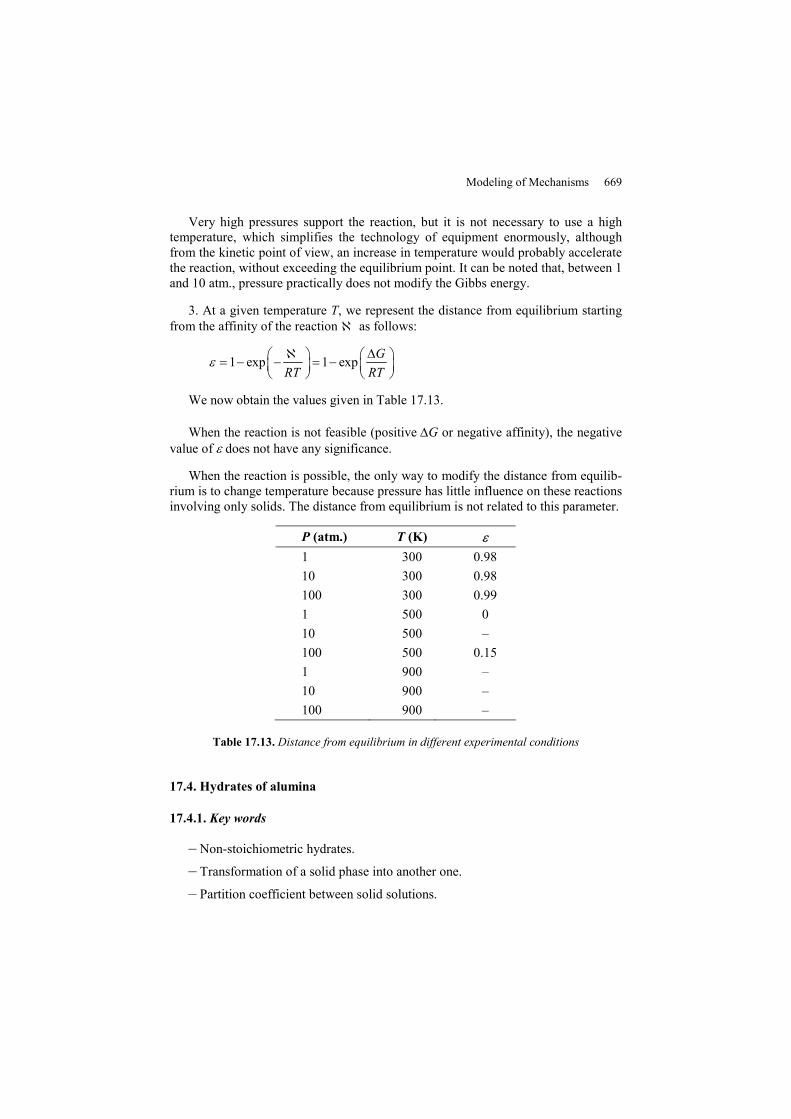
Very high pressures support the reaction, but it is not necessary to use a high temperature, which simplifies the technology of equipment enormously, although from the kinetic point of view, an increase in temperature would probably accelerate the reaction, without exceeding the equilibrium point. It can be noted that, between 1 and 10 atm., pressure practically does not modify the Gibbs energy.

3. At a given temperature T, we represent the distance from equilibrium starting from the affinity of the reaction ℵ as follows:

1 exp 1 exp GRT RT

ε ℵ Δ⎛ ⎞ ⎛ ⎞= − − = −⎜ ⎟ ⎜ ⎟⎝ ⎠ ⎝ ⎠

We now obtain the values given in Table 17.13.

When the reaction is not feasible (positive ΔG or negative affinity), the negative value of ε does not have any significance.

When the reaction is possible, the only way to modify the distance from equilib-rium is to change temperature because pressure has little influence on these reactions involving only solids. The distance from equilibrium is not related to this parameter.

P (atm.) T (K) ε 1 300 0.98 10 300 0.98 100 300 0.99 1 500 0 10 500 – 100 500 0.15 1 900 – 10 900 – 100 900 –

Table 17.13. Distance from equilibrium in different experimental conditions

17.4. Hydrates of alumina

17.4.1. Key words

– Non-stoichiometric hydrates. – Transformation of a solid phase into another one. – Partition coefficient between solid solutions.


17.4.2. Problem

We study equilibriums obtained between water vapor and boehmite for temperatures ranging between 250°C and 530°C [DAM 88].

For this, a sample is placed in a thermo-balance and heated to a first step of temperature at the highest water pressure. When the steady mass is reached, the pressure of water is decreased (by modifying the temperature of a cold point containing water) and we note the new step of mass. The operation is repeated with all the pressures. Then, the sample is brought up to a very high temperature (1,200°C) so as to eliminate all water and to obtain α-alumina (Al2O3), which is stable and can be cooled and weighed without absorbing water again. The experiments are started again at different temperatures. The amount of water still included in the solid (in moles of water per mole of alumina) is calculated for each step of pressure. The isobar curves are given in Figure 17.1.

The structural studies (X-rays diffraction and infrared spectroscopy) show that there is a phase change around 350°C and that if the high-temperature phase is a hydrated alumina (γ-alumina, Al2O3⋅xH2O), the low-temperature phase is an aluminum oxyhydroxide called boehmite, with formula AlOOH.

1. Boehmite is modeled just as a solid with three types of normal sites: Al O OHAl , O , and OH presenting two types of defects, OH vacancies and O2− ions, on OH sites: OH OHV and O° ′ .

Express the quasi-chemical reaction of water departure from boehmite. Consider that the concentration nB of ions OH− in equilibrium conditions can be represented by a line in a system of axis ( )B1/ ;1/n P . Calculate constant KB for this equilibrium at various temperatures and deduce from it the standard enthalpy and standard entropy of the reaction of boehmite dehydration.

2. We try to model the high-temperature phase of γ-alumina as a solid solution of substitution, hydroxide ions being substituted by oxygen ions. Express the quasi-chemical reaction of water departure. Consider that the model led to a concentration

An of hydroxide ions in equilibrium with water vapor, which agrees with the experimental results. Calculate the corresponding equilibrium constant KA and the enthalpy and entropy of γ-alumina dehydration.

3. Having modeled the two phases, we now model the transformation from one phase to the other phase. Express the quasi-chemical reaction of change of the boehmite phase into the γ-alumina phase by taking into account defects of each phase. Consider that there is a univariant system. Calculate the equilibrium constant of this change of the phase as a function of water pressure and the equilibrium constant of boehmite KB (constants KA and KB can be computed by extrapolation).


We can take into account the normal presence of divalent cation vacancies in γ-alumina because of its spinel structure.

4. Consider that this change of phase can be interpreted just as the partition of the hydroxides ions between the two solid phases. Calculate the partition coefficient. Deduce the standard enthalpy and entropy accompanying the partition.

17.4.3. Data

The pressure of the reference is 1 atm.

Table 17.14 and Figure 17.5 gives the temperature, the pressure, and the water content ε (moles of water per mole of alumina) for some equilibrium states.

Table 17.14. Water contents (in moles of water per mole of alumina) at various temperatures and water pressures

17.4.4. Solution

1. One gaseous water molecule is formed starting from two hydroxides according to the reaction:

OH OH OH 22OH V O H O° ′= + + [17.R.1]

The quantity ε represents the amount of water attached to 1 mole of alumina (i.e. with two aluminum atoms). Mole fraction of OH ions is thus twice more significant:

OH BOH 2n ε⎡ ⎤ = =⎣ ⎦

T (°C) P (Pa)

250 260 270 280 290 300 340 260 0.92 0.90 0.87 0.86 0.83 0.79 0.08 1,226 0.96 0.95 0.94 0.93 0.91 0.89 0.57 1,886 0.97 0.96 0.95 0.94 0.93 0.91 0.73 4,532 0.98 0.97 0.97 0.96 0.93 0.94 0.88 8,264 0.98 0.98 0.97 0.97 0.96 0.95 0.90 410 430 450 470 490 510 530 1,226 0.13 0.11 0.10 0.09 0.08 0.07 0.06 1,886 0.17 0.15 0.13 0.11 0.10 0.10 0.08


Figure 17.5. Isobaric curves of water content in boehmite

We represent the conservation of hydroxide sites (which shows that if ε varies from 0 to 1, nB varies from 0 to 2):

[ ] [ ]OH OH OHV O OH 2° ′⎡ ⎤ + + =⎣ ⎦

Taking into account the electric neutrality, it becomes:

[ ] BOH OH

1V O2n° −⎛ ⎞′⎡ ⎤ = = ⎜ ⎟⎣ ⎦ ⎝ ⎠

[ ][ ]

2B

OH OHB 2 2

BOH

1V O 2OH

n PPK

n

°⎛ ⎞−⎜ ⎟′⎡ ⎤⎣ ⎦ ⎝ ⎠= =

Now apply the law of mass action to reaction [17.R.1].

We deduce only one positive solution for nB, which is expressed as follows:

BB

22Pn

P K=

+ [17.21]

This relationship can still be expressed as follows:

B

B

1 12

Kn P

= + [17.22]


Figure 17.6. Representation of function [17.22] starting from the experimental data

In Figure 17.6, the reverse of Bn is drawn as a function of the reverse of the square root of the pressure (expressed in atm.). According to the model, we must obtain a line with intercept 0.5. It is noted that this result is correct except for the results obtained at 340°C. In the same manner, it can be shown that the model is not appropriate at higher temperatures.

Table 17.15 gives various constants resulting from the application of relation [17.22] to the experimental results. It is noted that the representative curve fits a line that passes through the point (0; 0.5), except for temperature 340°C. The value of the equilibrium constant is deduced from the slope of the straight lines of Figure 17.2 as follows: 2

B (slope) .K =

T (°C) Slope Intercept r2 KB

250 0.0021 0.501 0.993 4.55 × 10−6 260 0.0027 0.501 0.998 7.55 × 10−6 270 0.00378 0.499 0.993 1.43 × 10−5 280 0.0040 0.502 1.000 1.63 × 10−5 290 0.0051 0.502 0.999 2.56 × 10−5 300 0.0066 0.502 0.999 4.41 × 10−5 340 0.3702 −1.500 0.915

Table 17.15. Result of the modeling of boehmite


Figure 17.7. Variation of the equilibrium constant of boehmite with the temperature

According to Figure 17.7, the curve giving the logarithm of the equilibrium constant as a function of reverse of the temperature fits well a line since we find a correlation coefficient r2 = 0.982. We then calculate the slope of this line and its intercept as follows:

Slope = −12.98; intercept = 12.56

We thus admit that the variations in standard entropy and enthalpy that accompany the dehydration of boehmite are practically not temperature dependent.

From the slope of Figure 17.7, the standard enthalpy change can be computed as follows:

0B 12.98 1,000 107,931 J/moleH RΔ = × × = (endothermic water departure)

In the same way, starting from the intercept, we can obtain the standard entropy change as follows:

0B 12.56 104.5 J/mole KS RΔ = × =

2. Taking into account the assumed structure elements, the water departure from γ-alumina is written simply as follows:

O O O 22OH O V H O° °°= + + [17.R.2]

The application of the law of mass action to this equilibrium with the constant KA allows us to calculate the concentration nA of the OH− ions that are still present in γ-alumina. These concentrations are expressed in moles of OH− per mole of alumina, which gives:


A 2n ε=

We notice that, among the species that intervene in reaction [17.R.2], oxygen ions and oxygen vacancies are normally present in γ-alumina independent of the presence or absence of hydroxide ions. This leads us to neglect the variation in their activities in the course of dehydration. The law of mass action then leads to:

AA

PnK

= [17.23]

According to this model, amount An is proportional to the square root of the pressure. Figure 17.8 shows a good agreement. Table 17.16 gives the slopes and the corresponding coefficients of regression. Except for temperature 340°C (and in lower part), the experimental results fit well. From the slopes, the values of the equilibrium constants are computed at the various temperatures compatible with the model. Table 17.17 provides these values.

Figure 17.8. Proportionality in γ-alumina between the concentration of hydroxide ions and the square root of the pressure

T (°C)

340 410 430 450 470 490 510 530

Slope 4.93 2.45 2.14 1.88 1.62 1.46 1.41 1.15 r2 0.0375 0.998 0.994 0.999 1.000 1.000 0.987 0.997

Table 17.16. Slopes and coefficients of correlation of the lines in Figure 17.4


T (°C) KA 410 0.17 430 0.22 450 0.28 470 0.38 490 0.47 510 0.50 530 0.76

Table 17.17. Equilibrium constant for the dehydration of γ-alumina at various temperatures

Figure 17.9. Variations of the equilibrium constant for the dehydration of γ-alumina with temperature

Figure 17.9 gives a correct linear representation of the logarithm of the constant with the reverse of the temperature (r2 = 0.985) with a slope −6.598 and an intercept 7.867. From the slope and the intercept, we deduce the standard enthalpy and the standard entropy accompanying the departure of water from γ-alumina as follows:

0A 6.298 1,000 54,862 J/moleH RΔ = × × = (endothermic water departure) 0A 7.867 65.42 J/mole KS RΔ = × =

3. If reactions [17.R.1] and [17.R.2] give a good agreement with the results at temperatures lower than 300°C and higher than 400°C, respectively, it is clear that it is not the case within the intermediate range. We know, in addition, that the solid phase is not the same in these two domains. It is thus necessary to take into account a solid phase change that we must formulate starting from the various structural


characteristics of each phase. This change of structure can be represented by the following quasi-chemical reaction:

] ] ] ]' ° " °°Al O OH OH Al 2+ O OB B A AB B A A

2Al 2O O V 2Al V 3O V⎤ ⎤ ⎤ ⎤+ + + = + + +⎦ ⎦ ⎦ ⎦ [17.R.3]

where index B refers to boehmite phase and index A to γ-alumina. We can see that this reaction takes well into account the creation of bivalent cation vacancies necessarily present in γ-alumina of the spinel structure.

On applying the law of mass action to equilibrium [17.R.3], it gives with the same assumptions as in the case of γ-alumina:

[ ]OH OHB B

1

O VTK

°=

′ ⎡ ⎤⎣ ⎦

We must take into account the electric neutrality of boehmite and conservation of OH sites, so that:

' BOH OHB B

O V 12

n°⎡ ⎤ ⎡ ⎤= = −⎣ ⎦ ⎣ ⎦

We deduce:

B12 1

T

nK

⎛ ⎞= −⎜ ⎟⎜ ⎟

⎝ ⎠

But the hydroxide concentration in boehmite must also satisfy relation [17.19], which leads to:

2

B

B

22T

K PK

K

⎛ ⎞+= ⎜ ⎟⎜ ⎟

⎝ ⎠

Thus, during the change in structure, the system becomes univariant by the introduction of an expression represented by the equilibrium between the two solid phases, which means that if the pressure is fixed, this equilibrium occurs at a well-defined temperature.

We have calculated KT at various pressures and temperatures (Table 17.18) by extrapolating the values of KA and KB from the lines ln K = f(1/T) obtained from questions 1 and 2. Figure 17.10 gives the line ln KT versus 1/T thus obtained.


4. At the transformation equilibrium, there is, in fact, a superposition of three equilibriums [17.R.1], [17.R.2], and [17.R.3]. Any linear combination of these equilibriums is still equilibrium. To obtain a partition coefficient, it is necessary to find equilibrium that leads to the ratio /B An n that is a function of temperature only.

P (Pa) 267 1,220 1,866 4,532 P (atm.) 2.63 × 10−3 1.20 × 10−2 1.84 × 10−2 4.47 × 10−2 T (K) 598 615 623 633 KB 1.07 × 10−4 1.95 × 10−4 2.56 × 10−4 3.56 × 10−4 KA 0.04 0.06 0.07 0.08 KT 12.11 24.27 27.46 43.64 nB 1.43 1.59 1.62 1.7 nA 0.25 0.46 0.53 0.76

Table 17.18. Characteristics for the equilibrium of change of phase of the from boehmite to the γ-alumina phase

Figure 17.10. Variations in the equilibrium constant of the transformation of bœhmite phase into γ -alumina phase with temperature

Examine the following linear combination:

[ ] [ ] [ ] [ ]17.R.1 17.R.2 17.R.317.R.4

2 2 2= − −

It leads to the reaction:

] ] ] ]" °Al 2 O O Al OH OA A B BA A B

2Al V 2O 2OH 2Al 2OH 2O+⎤⎤ ⎤+ + + = + +⎦ ⎦ ⎦ [17.R.4]


And applying the law of the mass action, it gives:

B A

A BP

T

n KK

n K K= =

Thus, the constant KP is a true partition coefficient and its existence reveals the equality between the chemical potentials of OH in the two phases:

B B A Aln lnRT n RT nμ μ° °+ = +

Therefore,

B A B

A

exp Pn

Kn RT

μ μ° °−= =

The standard enthalpy and entropy result from the standard enthalpies and entropies of the reactions in the same linear combination, or:

0 0 0 0B A0.5 0.5 0.5 29.82 kJ/moleP TH H H HΔ = Δ − Δ − Δ = −

We have an exothermic reaction in the direction chosen for reaction [17.R.4]

0 0 0 0B A0.5 0.5 0.5 84.21 J/mole KP TS S S SΔ = Δ − Δ − Δ = −

17.5. Point defects in a metal sulfide

17.5.1. Key words

– Defining and connecting Brouwer domains. – Computation of the concentrations of point defects in a semiconductor as a

function of gas pressure. – Effect of doping with foreign cations of higher valence.

17.5.2. Problem

See the equilibrium of the defects of a metal sulfide MS with sulfur vapor at temperature 1,246 K.


1. Complete the following quasi-chemical reactions between the defects of a metal sulfide.

M0 ?V= + [17.Eq.1]

? e h′= + ° [17.Eq.2]

M? h V ′= ° + [17.Eq.3]

S? V e° ′= + [17.Eq.4]

gas2 M?S V= + [17.Eq.5]

2. Express, according to the various equilibrium constants Ki and the pressure of di-sulfur vapor, the approximate expressions for the concentrations of the various point defects and consider the range of validity of these expressions in the pressure space.

3. Consider the range of pressure between 10−3 and 2 mmHg. Compute the equilibrium constants Ki for i varying from 1 to 5. Calculate the concentrations of the various point defects by specifying the ranges of validity. Deduce the corresponding Kröger-Vink diagram.

4. What range of pressures can we be satisfied with a Wagner approximation? 5. Compute, the constant K6 of the following equilibrium:

'M S0 V V °= + [17.Eq.6]

6. Substitute Sn4+ ions for M2+ ions into the preceding metal sulfide with the concentration C = 0.15 at temperature 1,246 K and under the di-sulfur pressure of 0.1 mmHg. Compute the concentrations of the various defects.

17.5.3. Data

Data are gathered in Table 17.19 (1 atm. = 760 mmHg)

Equilibrium K (mole fract. atm.) ΔH° (eV/atom) 1 6.00 × 10−3 2.50 2 1.73 × 10−3 0.70 3 7.40 × 10−2 0.14 4 7.40 × 10−2 0.14 5 2.50 × 10−4 0.50

Table 17.19. Data of various equilibriums of the point defects of sulfide MS


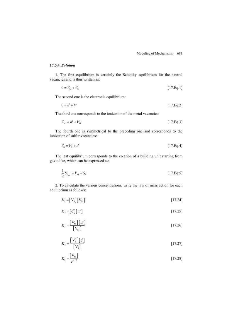
17.5.4. Solution

1. The first equilibrium is certainly the Schottky equilibrium for the neutral vacancies and is thus written as:

M S0 V V= + [17.Eq.1]

The second one is the electronic equilibrium:

0 e h′= + ° [17.Eq.2]

The third one corresponds to the ionization of the metal vacancies:

M MV h V ′= ° + [17.Eq.3]

The fourth one is symmetrical to the preceding one and corresponds to the ionization of sulfur vacancies:

S SV V e° ′= + [17.Eq.4]

The last equilibrium corresponds to the creation of a building unit starting from gas sulfur, which can be expressed as:

gas2 M S12

S V S= + [17.Eq.5]

2. To calculate the various concentrations, write the law of mass action for each equilibrium as follows:

[ ] [ ]1 S MV VK = [17.24]

[ ] [ ]2 e hK ′= ° [17.25]

[ ] [ ][ ]M

3M

V hV

K′ °

= [17.26]

[ ][ ]S

4S

V e

VK

° ′⎡ ⎤⎣ ⎦= [17.27]

[ ]M5 1/ 2

VK

P= [17.28]


With these equations, add the expression of the electric neutrality:

[ ] [ ] [ ]M SV e h V°′ ′ ⎡ ⎤+ = ° + ⎣ ⎦ [17.29]

Thus, we obtain six equations with six unknown factors that are the concentrations of the defects: [ ] [ ] [ ] [ ] [ ]M S M Se , h , V , V , V , and V°′ ′ ⎡ ⎤° ⎣ ⎦ . So, we can calculate these concentrations as functions of equilibrium constants and pressure P of di-sulfur.

To carry out calculation, we consider the Brouwer approximation, which consists of keeping only a single term of each sign in the expression of the electric neutrality.

Case BR 1 BR 2

[ ]MV 1/ 25K P 1/ 2

5K P

[ ]SV 11/ 2

5

KK P

11/ 2

5

KK P

[ ]e ' 1/ 2 1/ 2

1 2 4

3 5

K K K PK K

−⎛ ⎞⎜ ⎟⎝ ⎠

1/ 22K

[ ]h° 1/ 2

1/ 22 35

1 4

K KK P

K K⎛ ⎞⎜ ⎟⎝ ⎠

1/ 22K

SV°⎡ ⎤⎣ ⎦ 1/ 2

1 3 4

2

K K KK

⎛ ⎞⎜ ⎟⎝ ⎠

1/ 2

1 41/ 22 5

K K PK K

−

'MV⎡ ⎤⎣ ⎦

1/ 2

1 3 4

2

K K KK

⎛ ⎞⎜ ⎟⎝ ⎠

1/ 2

3 51/ 22

K K PK

Domain 1 2R P R< < 2 1R P R< <

Table 17.20. Defect concentrations in BR 1 and BR 2 domains

We can thus consider four Brouwer cases:

Case BR 1 [ ]M SV V°′ ⎡ ⎤= ⎣ ⎦ with the approximations: [ ] [ ]'M SV e and V h°′⎡ ⎤ ⎡ ⎤> > °⎣ ⎦ ⎣ ⎦

Case BR 2 [ ] [ ]e h′ = ° with the approximations: [ ] [ ]'M SV e and V h°′⎡ ⎤ ⎡ ⎤< < °⎣ ⎦ ⎣ ⎦


Case BR 3 [ ] [ ]MV h′ = ° with the approximations: [ ] [ ]'M SV e and V h°′⎡ ⎤ ⎡ ⎤> < °⎣ ⎦ ⎣ ⎦

Case BR 4 [ ] Se V°′ ⎡ ⎤= ⎣ ⎦ with the approximations: [ ] [ ] [ ]M SV e and V h°′ ′ ⎡ ⎤< > °⎣ ⎦

For a given approximation, the concentrations of the neutral species remain identical since these species are not involved in the expression of the electric neutrality.

Case BR 3 BR 4

[ ]MV 1/ 25K P 1/ 2

5K P

[ ]SV 11/ 2

5

KK P

11/ 2

5

KK P

[ ]e' 1/ 421/ 2 1/ 23 5

KP

K K−

1/ 21/ 41 4

5

K KP

K−⎛ ⎞

⎜ ⎟⎝ ⎠

[ ]h° 1/ 2 1/ 43 5( )K K P

1/ 21/ 45

21 4

KK P

K K⎛ ⎞⎜ ⎟⎝ ⎠

SV°⎡ ⎤⎣ ⎦ 1/ 2

1/ 431 4

2 5

KK KP

K K−⎛ ⎞

⎜ ⎟⎝ ⎠

1/ 2

1/ 41 4

5

K KP

K−⎛ ⎞

⎜ ⎟⎝ ⎠

'MV⎡ ⎤⎣ ⎦ 1/ 2 1/ 4

3 5( )K K P ( )1/ 21 4 5 3 1/ 4

2

K K K KP

K

Domain 2 1andP R P R> > 1 2andP R P R< <

Table 17.21. Defect concentrations in BR 3 and BR 4 domains

For each Brouwer case, we substitute the values of the concentrations in the corresponding inequalities. We can then define two critical pressures:

22

13 5

KR

K K⎛ ⎞

= ⎜ ⎟⎝ ⎠

[17.30]

2

1 42

2 5

K KR

K K⎛ ⎞

= ⎜ ⎟⎝ ⎠

[17.31]

We represent the ranges of validity of the expressions in the tables.


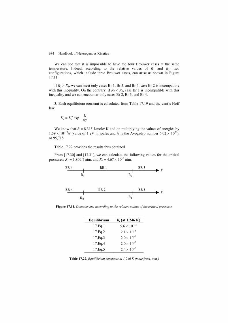
We can see that it is impossible to have the four Brouwer cases at the same temperature. Indeed, according to the relative values of R1 and R2, two configurations, which include three Brouwer cases, can arise as shown in Figure 17.11.

If R2 > R1, we can meet only cases Br 1, Br 3, and Br 4; case Br 2 is incompatible with this inequality. On the contrary, if R2 < R1, case Br 1 is incompatible with this inequality and we can encounter only cases Br 2, Br 3, and Br 4.

3. Each equilibrium constant is calculated from Table 17.19 and the vant’s Hoff law:

0 expi iEK K

RT= −

We know that R = 8.315 J/mole/ K and on multiplying the values of energies by 1.59 × 10−19N (value of 1 eV in joules and N is the Avogadro number 6.02 × 1023), or 95,718.

Table 17.22 provides the results thus obtained.

From [17.30] and [17.31], we can calculate the following values for the critical pressures: R1 = 1,809.7 atm. and R2 = 4.67 × 10−6 atm.

Figure 17.11. Domains met according to the relative values of the critical pressures

Equilibrium Ki (at 1,246 K) 17.Eq.1 5.6 × 10−13

17.Eq.2 2.1 × 10−6

17.Eq.3 2.0 × 10−2

17.Eq.4 2.0 × 10−2 17.Eq.5 2.4 × 10−6

Table 17.22. Equilibrium constants at 1,246 K (mole fract. atm.)


Figure 17.12. Kröger-Vink’s diagram between 0.001 and 2 mmHg at 1,246 K

R2 being smaller than R1, we are clearly, according to Figure 17.1, in the lower case for which only ranges Br 4, Br 2, and Br 3 exists.

The range of pressure lying between 10−3 and 2 mmHg corresponds to the range between 1.32 × 10−6 and 2.6 × 10−3 atm. (i.e. around R2). We encounter only case Br 4 for the low pressures and case Br 2 for the highest pressures. From the expressions in Tables 17.20, 17.21 and 17.22, we calculate the values of the concentrations that we deferred in Table 17.23.

From Table 17.23, we can plot the Kröger-Vink diagram, which represents the logarithms of the concentrations versus the logarithm of the pressure. Figure 17.12 gives this diagram.

4. On the left of the diagram, we can regard as prevalent the sulfur vacancies SV ° and electrons (of same concentrations), which consists, under these conditions,

of metal sulfide, a n-type Wagner semiconductor with ionized anion vacancies and free electrons. The approximation is much better than that when the sulfur pressure is lower.

5. On carrying out the following linear combination of equilibriums [17.Eq.1] + [17.Eq.3] + [17.Eq.4] − [17.Eq.2], we find equilibrium [17.Eq.6]. The constant is thus obtained as follows:

101 3 46

2

1.08 10K K K

KK

−= = ×

6. We now consider the case of doping with tin. Equations [17.24] to [17.28] are still applicable, and it is necessary to add the tin concentration PbSn .C°°⎡ ⎤ =⎣ ⎦


P (mmHg) [ ]′ 0,1MV VS VM

0.001 5.40 × 10−8 1.98 × 10−4 2.83 × 10−9 0.003 7.11 × 10−8 1.14 × 10−4 4.90 × 10−9 R2 7.42 × 10−8 1.05 × 10−4 5.33 × 10−9 0.005 8.80 × 10−8 8.84 × 10−5 6.32 × 10−9 0.01 1.24 × 10−7 6.25 × 10−5 8.94 × 10−9 0.05 2.78 × 10−7 2.80 × 10−5 2.00 × 10−8 0.1 3.93 × 10−7 1.98 × 10−5 2.83 × 10−8 0.5 8.80 × 10−7 8.84 × 10−6 6.32 × 10−8 1 1.24 × 10−6 6.25 × 10−6 8.94 × 10−8 2 1.76 × 10−6 4.42 × 10−6 1.26 × 10−7

P (mmHg) e′ h° SV °

0.001 2.00 × 10−3 1.06 × 10−3 2.00 × 10−3 0.003 1.50 × 10−3 1.39 × 10−3 1.52 × 10−3 R2 1.45 × 10−3 1.45 × 10−3 1.46 × 10−3 0.005 1.45 × 10−3 1.45 × 10−3 1.23 × 10−3 0.01 1.45 × 10−3 1.45 × 10−3 8.7 × 10−4 0.05 1.45 × 10−3 1.45 × 10−3 3.89 × 10−4 0.1 1.45 × 10−3 1.45 × 10−3 2.75 × 10−4 0.5 1.45 × 10−3 1.45 × 10−3 1.23 × 10−4 1 1.45 × 10−3 1.45 × 10−3 8.70 × 10−5 2 1.45 × 10−3 1.45 × 10−3 6.15 × 10−5

Table 17.23. Defect concentrations

But now the electric neutrality takes the following form:

[ ] [ ]'M SV e' h V 2C°⎡ ⎤ ⎡ ⎤+ = ° + +⎣ ⎦ ⎣ ⎦

We find the four preceding Brouwer cases to which two new cases must be added, cases Br 6 and Br 7, defined by:

BR 6: [ ]e ' 2C= BR 7: [ ]MV 2C′ = .


Case BR 6 BR 7

[ ]MV 1/ 25K P 1/ 2

5K P

[ ]SV 11/ 2

5

KK P

11/ 2

5

KK P

[ ]e′ 2C 21/ 2

3 5

2K CK K P

[ ]h° 2

2KC

1/ 2

3 5

2K K P

C

SV°⎡ ⎤⎣ ⎦ 1 41/ 2

52K K

K CP 1 3 4

22K K K

K C

'MV⎡ ⎤⎣ ⎦

1/ 23 5

2

2K K CPK

2C

Table 17.24. Defect concentrations with high tin concentrations

Table 17.24 gives the expressions of the defect concentrations in these two cases.

Now examine the conditions for the application of cases Br 6 and Br 7. Table 17.25 provides these conditions by dividing each case into two sub-cases. These conditions reveal for a given pressure, four remarkable tin concentrations that are given for pressure 0.1 mmHg or 1.32 × 10−4 atm.:

1/ 2

1 41 1/ 2

5

0.000324

K KC

K P⎛ ⎞

= =⎜ ⎟⎝ ⎠

1/ 2

22 0.00073

4K

C ⎛ ⎞= =⎜ ⎟⎝ ⎠

1/ 261 3 4

32

5.20 104

K K KC

K−⎛ ⎞

= = ×⎜ ⎟⎝ ⎠

1/ 2

53 54 1.20 10

4K K P

C −⎛ ⎞= = ×⎜ ⎟

⎝ ⎠

Only sub-case BR 6/2 is entirely satisfied, which makes it possible to calculate concentrations according to Table 17.24 (central column) and are given in Table 17.26.

Thus, doping with tin under these conditions ( 0.018C > , P = 0.1 mmHg, and T = 1,264 K) allows to increase and control the free electrons content.


Case Condition Domains Conclusion

[ ] [ ]Me V′ ′> P < < R1 No

BR 6/1 [ ]SV h°⎡ ⎤ > °⎣ ⎦ P < < R2 No

S2 VC °⎡ ⎤> ⎣ ⎦ C > > C1 = 0.035 Yes

[ ] [ ]Me V′ ′> P < < R1 Yes

BR 6/2 [ ]SV h°⎡ ⎤ < °⎣ ⎦ P > > R2 Yes

[ ]2 hC > ° C > > C2 = 0.018 Yes

[ ] [ ]Me V′ ′< P > > R1 No

BR 7/1 [ ]SV h°⎡ ⎤ > °⎣ ⎦ P < < R2 No

S2 VC °⎡ ⎤> ⎣ ⎦ C > > C3 = 0.077 Yes

[ ] [ ]Me V′ ′< P > > R1 No

BR 7/2 [ ]SV h°⎡ ⎤ < °⎣ ⎦ P > > R2 Yes

[ ]2 hC > ° C > > C4 = 0.041 Yes

Table 17.25. Conditions of validity of the various domains doped with tin

VS 1.98 × 10−5 VM 2.83 × 10−8 e′ 0.3 h° 7.10 × 10−6

SV ° 1.34 × 10−6

MV ′ 8.09 × 10−5

Table 17.26. Defect concentrations for a tin concentration of 0.15, at pressure and temperature of 0.1 mmHg and at 1,246 K, respectively


17.6. Point defects of an alkaline bromide

17.6.1. Key words

– Point defects of a Schottky solid. – Brouwer approximation. – Kröger-Vink diagrams.

17.6.2. Problem

An alkaline bromide MBr is considered at equilibrium with bromide vapor within a pressure range between 10−5 and 0.1 atm. and at 600°C.

1. Calculate at the indicated temperature the equilibrium constants for reactions [17.R.5] to [17.R.11].

2. Calculate the pre-exponential factor and the enthalpies for reactions [17.R.12] and [17.R.13].

3. Give the expressions of the concentrations of the various defects in the considered range of pressure. Show that in this range bromide is clearly a Schottky solid with ionized vacancies. Plot the Kröger-Vink diagram for the four major defects within the considered pressure range.

17.6.3. Data

Table 17.27 and reactions [17.R.12] and [17.R.13] are given as follows:

M Br0 V V= + [17.R.12]

M 2 Br10 ( )2

V V= + [17.R.13]

17.6.4. Solution

1. To calculate, for each reaction, the equilibrium constant at 600°C (i.e. at 873 K), we apply the vant’s Hoff law:

0 expi iHK K

RTΔ⎛ ⎞= −⎜ ⎟

⎝ ⎠ [17.32]


Reaction 0K (atom fract. atm.) ΔH° (eV/molecule)

M Br0 V V °′= + [17.R.5] 1,000 2.2

M MV V h′= + ° [17.R.6] 2 1.08

Br BrV V e° ′= + [17.R.7] 2 1,8

0 e h′= + ° [17.R.8] 9.3 6.9

( )M M 22V V= [17.R.9] 6 −1.5

( )Br Br 22V V= [17.R.10] 6 −0.19 1

2 2 Br MBr Br V= + [17.R.11] 0.11 1.09

Table 17.27. Pre-exponential factors and enthalpies of some quasi-chemical reactions in an alkaline bromide

For this, we consider the perfect gas constant: R = 8.315 J/mole K.

If Avogadro number N is 6.02 × 1023, to transform the eV/atom given into J/mole, we multiply the value of enthalpy given in Table 17.1 by 1.59 × 10−19 N or 95,718.

Table 17.28 provides the results thus obtained. We especially note the very low value of the constant K8 of the electronic equilibrium, which assumes that the bromide under study is probably not an electronic semiconductor, which is confirmed by the high value of the gap ( 4H °Δ ) in Table 17.27.

Reaction Ki (600°C)

[17.R.5] K5 = 2.52 × 10−10 [17.R.6] K6 = 1.31 × 10−6

[17.R.7] K7 = 9.84 × 10−11

[17.R.8] K8 = 2.85 × 10−39 [17.R.9] K9 = 2.33 × 109

[17.R.10] K10 = 73.5 [17.R.11] K11 = 6.30 × 10−8

Table 17.28. Values of independent equilibrium constants of quasi-chemical reactions related to alkaline bromide


2. At first, examine the case of equilibrium [17.R.12]. It results from the following linear combination of equilibriums [17.R.5], [17.R.6], [17.R.7] and [17.R.8]:

[ ] [ ] [ ] [ ] [ ]17.R.12 17.R.5 17.R.8 17.R.6 17.R.7= + − −

Then, we can compute the enthalpy of reaction [17.R.12] as the result of the same linear combination of the enthalpies of the four concerned reactions.

The equilibrium constant (and the pre-exponential factor) is then obtained by a relationship of the form:

5 812

6 7

K KK

K K=

In the same way, equilibrium [17.R.13] is the result of the following linear combination:

[ ] [ ] [ ]117.R.13 17.R.12 17.R.92

= −

We apply this combination to the enthalpies to calculate the enthalpy of the reaction. For the equilibrium constant (and the pre-exponential factor), we use the relationship:

1213

9

KKK

=

These relationships make it possible to derive values given in Table 17.29.

K° (atom fract. atm.) ΔH° (eV/atom) K

[17.R.12] 2,325 6.22 K12 = 5.58 × 10−33

[17.R.13] 949 6.97 K13 = 1.15 × 10−37

Table 17.29. Non-independent equilibrium constants

3. We calculate the concentrations of eight defects and represent seven expressions of the law of mass action for equilibriums [17.R.5] to [17.R.11] to which we add the electric neutrality as follows:

[ ] [ ]M Bre' V h V° °′ ⎡ ⎤ ⎡ ⎤+ = +⎣ ⎦ ⎣ ⎦


Defect Concentration Defect Concentration

MV 11K P e′ 8 5

6 11

K KK K P

BrV 5 8

6 7

K KK K P

h° 6 11

5

K K PK

M 2( )V 29 11K K P MV ′ 5K

Br 2( )V 2 210 5 82 2 26 7 11

K K KK K K P

°BrV 5K

Table 17.30. Expressions of the concentrations of point defects in a Brouwer domain

To simplify our calculation, we use the Brouwer method. We can define four Brouwer domains as follows:

[ ]M BrV V°′ ⎡ ⎤= ⎣ ⎦ [ ] Bre V°′ ⎡ ⎤= ⎣ ⎦ [ ]MV h°′ ⎡ ⎤= ⎣ ⎦ and [ ]e h°′ ⎡ ⎤= ⎣ ⎦

Taking into account the character very far away from the semiconductors of the metal bromide under study, we start with the first domain. It leads to the expressions given in Table 17.30 for the various concentrations.

Now examine the conditions for the application of our approximation. By examination of the electric neutrality, the following conditions are observed:

[ ] [ ]MV e′ ′>> and BrV h° °⎡ ⎤ ⎡ ⎤>>⎣ ⎦ ⎣ ⎦

which is transformed, reporting the values of the concentrations in these two

inequalities, into:28

1 2 26 11

KP P

K K>> = and

25

2 2 26 11

KP P

K K<< = .

On calculating P1 and P2 numerically, starting from the constants given in Table 17.28, we obtain the following conditions:

511.20 10 9,360,000P−× << <<

We can then calculate the concentrations of the various defects at 600°C and for various oxygen pressures. Results are given in Table 17.31.

It is clear that most defects are ionized metal vacancies and ionized bromine vacancies. So, this alkaline bromide is a Schottky solid. This result appears even


more clearly in Figure 17.13, which gives the Kröger-Vink diagram for the four major defects in the pressure range. The ionized metal vacancies and bromine vacancies are the most important defects and are present in equal amounts.

P ′MV °BrV VM

0.00001 1.6 × 10−5 1.6 × 10−5 2.0 × 10−10

0.0001 1.6 × 10−5 1.6 × 10−5 6.3 × 10−10 0.001 1.6 × 10−5 1.6 × 10−5 2.0 × 10−9 0.01 1.6 × 10−5 1.6 × 10−5 6.3 × 10−9 0.1 1.6 × 10−5 1.6 × 10−5 2.0 × 10−8 (VM)2 (VBr)2 e′ 0.00001 9.3 × 10−11 5.8 × 10−44 1.7 × 10−28

0.0001 9.3 × 10−10 5.8 × 10−45 5.5 × 10−29 0.001 9.3 × 10−9 5.8 × 10−46 1.7 × 10−29 0.01 9.3 × 10−8 5.8 × 10−47 5.5 × 10−30 0.1 9.3 × 10−7 5.8 × 10−48 1.7 × 10−30

Table 17.31. Concentrations of point defects in alkaline bromide at 600°C

Figure 17.13. Kröger-Vink’s diagram for the four major defects of alkaline bromide

at 600°C between 10−5 and 0.1 atm


17.7. Diffusion of a metal into another metal

17.7.1. Key words

– Determination of a diffusion coefficient. – Application of the second Fick law. – Influence of temperature on diffusion.

17.7.2. Problem

A bar of a metal A is placed end to end with another metal B.

Both bars are heated at a certain temperature T during a sufficient time t. Atoms of A diffuse inside B. After rapid cooling to the ordinary temperature, the bar of B is cut in sections of 1 mm thickness; the X-coordinate is taken in the middle of each section. Element A is analyzed in each section. We thus obtain the concentration of A (in mole/cm3) according to the X-coordinate in B after diffusion.

The experiment is performed again at various temperatures.

1. Assuming the exchange reaction at the interface A/B to be very fast compared with the diffusion. Calculate the concentration of elements A and B at the interface. Also, calculate the diffusion coefficient of A in B at the various temperatures. Show the agreement between the measurements and the results of calculation. Show that the length of the bar of B is sufficient to justify the model.

T (K) X-coordinate (m)

1,106 1,143 1,158 1,208 0.002 0.047 0.048 0.048 0.048 0.004 0.046 0.046 0.047 0.047 0.010 0.041 0.043 0.043 0.044 0.040 0.022 0.026 0.027 0.031 0.070 0.009 0.013 0.015 0.020 0.100 0.003 0.006 0.007 0.012 0.130 0.001 0.002 0.003 0.006 0.150 0.000 0.001 0.001 0.004

Table 17.32. Concentrations of A at different points after maintenance at various temperatures


2. Give an expression of the diffusion coefficient as a function of temperature; deduce the energy of activation of diffusion.

3. Compute the length of the diffusion jump of A in B.

17.7.3. Data

Both solids A and B crystallize in the same system. A and B are miscible in all proportions and the formed solution is perfect. The bar of B is 40 cm in length. The time of temperature maintenance is 108 s.

Table 17.32 gives the result of the concentration of A at different temperatures for various X-coordinates in B in mole/cm3. Table 17.33 provides some data concerning both metals.

The standard entropy at 298 K (independent of the temperature) for both pure solids A and B is 540 J/mole K.

B A

ρ (g/cm3) 10.5 19.3 M 108 197

Table 17.33. Densities and molar masses of metals A and B

17.7.4. Solution

1. We consider, as shown in Figure 17.14, a one-way diffusion of A, along the axis Ox in the bar of B.

At the initial time, a certain amount of A will be dissolved at the surface of B; conversely, a certain amount of B is dissolved in the bar of A. We assume that the exchange reaction at the interface is very fast compared with the diffusion and thus at the initial time an interfacial equilibrium is established. Fix the concentration C0 of A in the bar of B at x = 0.

Represent the conservation of the atoms of A in a small volume surrounding the interface, and the sum of the mole fractions of A in A and of A in B is equal to 1:

0 0A(A) A(B) 1x x+ = [17.33]


We represent the equilibrium of the element of A between the two phases by the equality of the chemical potentials of A in the two bars:

0 0A(B) A(A)μ μ=

Formulate the chemical potentials. It becomes:

0 0 0 0A(A) A(B) A(B) A(A)ln( ) ln( )g RT x g RT x+ = +

where 0 0A(A) A(B)andg g are the standard Gibbs energy of pure solid A in the

crystalline system of A and the crystalline system of B, respectively.

Then,

0 0 0A(A) A(B) A(A)0A(B)

expx g g

KRTx−

= = [17.34]

Figure 17.14. Device for the study of diffusion of A in B

Combining [17.33] and [17.34], we obtain the atomic fraction of A in B:

0A(A)

11

xK

=+

[17.35]

To calculate K, we consider again expression [17.34]. The Gibbs energy of a pure element is (corresponding enthalpy being null):

0 0A(A) A(A)g Ts= −

For a pure element of A in a phase of B (hypothetical situation), we can also take a null enthalpy because the solution is perfect (there is no mix enthalpy). Thus, we have:

0 0A(B) A(B)g Ts= −


Thus, constant K becomes:

0 0A(A) A(B)exp

s sK

R−

=

The entropies of formation of pure solids A and B are identical, it is probable that the entropy of formation of pure solid A in the network of B is about the same because the crystalline system of the two phases are the same and the solution is perfect. Thus, we can pose:

0 0A(A) A(B)s s= and 1K =

And substituting into [17.35], we obtain:

0A(B) 0.5x =

The concentration C0 of A in B at the interface is thus:

0A(B)

0M M

0.5xC

V V= = [17.36]

VM is the molar volume of the equimolar solid solution. As this solution is perfect, there is an additive property of the molar volumes balanced by the atomic fractions; thus:

A B

3A BM M M

A B

0.5 0.5 0.5 0.5 10.24 cm /moleM M

V V Vρ ρ

= + = + =

The application of [17.36] gives C0 = 0.0488 mole/cm3.

We now study the diffusion in the bar of B by applying the second law of Fick along an axis, which is represented as follows:

2

2

C CDt x

∂ ∂=

∂ ∂ [17.37]

In this equation, C represents the concentration of the diffusing species (here A) at X-coordinate x (in the bar of B) at time t.

This is a second-order partial differential equation. Its resolution gives the fun-ction C(x, t) of the concentration of A at time t and at X-coordinate x in the bar of B.


To solve this equation, we require the knowledge of the boundary conditions.

We first consider diffusion in a semi-infinite medium and justify this assumption by ensuring later that element A does not reach the end of the bar of B.

Thus, the boundary conditions of [17.37] is as follows:

0 < x < ∞

0if 0 and 0, thent x C C> = =

if 0 and 0, then 0t x C= > =

The solution of this equation (see Appendix 10 section A.10.4.1) is then, if erf(u) is the error function (see Appendix 10 section A.10.1):

0

1 erf2

C xC Dt

⎛ ⎞= − ⎜ ⎟

⎝ ⎠ [17.38]

To compute the diffusion coefficient D that cannot be clarified from [17.38], we consider the equivalence of the function erf(u) when u approaches 0, which is (see

Appendix 10 section A.10.1.4): 2erf ( )πuu ≈ .

On applying this equivalence to the smallest value of the X-coordinate: x1 = 0.002 m, we have:

1 1

0

1π

C xC Dt

≈ − [17.39]

Therefore, we deduce a value of the diffusion coefficient (in m2/s) if x1 (in m) and t (in s):

21

2

1

0

π 1

xDCtC

=⎛ ⎞

−⎜ ⎟⎝ ⎠

[17.40]

Considering expression [17.40] for the various temperatures, we obtain Table 17.34, which gives the diffusion coefficients at various temperatures.

We have now to verify that our model and equation [17.38] are correct. For this, we initially verify the assumption that the semi-infinite bar is good. It is necessary


that the bar of B is rather long so that A does not reach the end of the bar of B at the end of the experiment. We verify that for x = 0.40 and the highest temperature (1,208 K), the ratio of the concentrations given by [17.38] is very low (3.6 × 10−6).

T (K) D (m2/s)

1,106 1.40 × 10−11

1,143 2.03 × 10−11 1,158 2.35 × 10−11 1,208 3.73 × 10−11

Table 17.34. Diffusion coefficients of A in B at various temperatures

Then, we seek the quality of the linear regression between the measured values

of ratio C/C0 and the computed ones from the function 1 erf2

xDt

⎛ ⎞− ⎜ ⎟

⎝ ⎠.

Table 17.35 shows good agreement with the computed values since the slope of the corresponding least-square line has a slope of 1 with intercept 0.

We can also confirm this agreement comparing the calculated curves of the ratio of the concentrations and the experimental curves. Figure 17.15 gives the example for such a comparison at temperature 1,158 K.

T (K) Slope Intercept

1,106 1.0 0.000 1,143 1.0 0.000 1,158 1.0 0.000 1,208 1.0 0.000

Table 17.35. Characteristics of the least-square line

2. It is known that a priori a diffusion coefficient obeys the Arrhenius law. We thus expect a law of the form:

0 exp AD DT

⎛ ⎞= ⎜ ⎟⎝ ⎠

[17.41]


To verify this law, we calculate, starting from Table 17.34, the logarithm of diffusion coefficient from the plot versus the reverse of absolute temperature.

Figure 17.16 shows that the experimental points fit well with a line obeying the Arrhenius law.

The equation of the least-square line is as follows:

12,856n 13.37AD BT T

= + = − −

Figure 17.15. Theoretical and experimental plots of concentration of A as a function of the X-coordinate

Figure 17.16. The Arrhenius line for diffusion coefficient

From which we can have the following expression:

60

12,856exp 1.56 10 expAD DT T

− −⎛ ⎞ ⎛ ⎞= = ×⎜ ⎟ ⎜ ⎟⎝ ⎠ ⎝ ⎠


It is known that the temperature coefficient is associated with the energy of activation of diffusion by:

106,900 J/mole or 107 kJ/moleE AR= − =

3. The pre-exponential factor D0 is defined in the model of jumps (see section 5.3.1.1) by:

2

0 2a kTD

h=

where a is the distance between two equilibrium positions of the diffusing particle; k and h the Boltzmann and Planck constants, respectively; and T an average temperature at a given temperature (i.e. 1,154 K). Calculation leads to a = 3.59 × 10−10 m or 3.59 Å.

17.8. Generation of atmospheres with very low pressures

17.8.1. Key words

– Calculation of the conditions to obtain a very low pressure of a permanent gas. – Obtaining controlled water vapor pressures. – Study of homogenous equilibriums in the gas phase. – Study of heterogenous equilibriums.

17.8.2. Problem

We want to generate various atmospheres in an enclosure, around a solid sample.

1. We generate a water pressure by connecting the reactor to a thermo-stated tank containing distilled water. The whole of gas circuit can be treated in such a way that the coldest point of the whole gas circuit is at a maximum of +40°C.

Determine the range of water pressures that we can ensure in the reactor. Give some comments suggested by these results.

2. We now wish to generate very low pressures of oxygen. For this, we introduce into the reactor a mixture of gas composed either of hydrogen and water vapor or of carbon dioxide and carbon monoxide at a total pressure of 1 atm. Knowing that the pressure ratio of two permanent gases that it is possible to ensure in the reactor is


between 10−3 and 103 atm. (A gas can be introduced with pressures ranging between 10−3 and 1 atm.; the total pressure not exceeding the atmospheric pressure.) Calculate the range of oxygen pressure that each one of these two mixtures can ensure. Which remarks suggest this method in the case of kinetic studies?

3. We now suggest carrying out in a bulb connecting the reactor the equilibrium of dissociation of an oxide with its metal in a solid state. Show that the use of nickel oxide makes it possible to cover a range of oxygen pressure comparable with that used in the preceding devices. Give some critiques of the method in the case of its use for kinetic measurements.

17.8.3. Data

Energies are expressed in joules and temperatures in degree Kelvin. The data of Tables 17.36 and 17.37 are assumed to be independent of temperature.

– The lowest temperature of regulation: −40°C. – Melting point of nickel: 1,455°C. – Temperature of the reactor: 1,000 K.

Transformation ΔH°

H2O liquid → vapor 40,838

H2O solid → liquid 1,379

Table 17.36. Enthalpies of transformation of water at the temperature of the change of state under 1 atm.

17.8.4. Solution

At first, we observe that no data are provided about the molar heat capacities of the components or about their variations with temperature. Consequently, we assume that the standard enthalpies and entropies do not vary with temperature between two state changes.

1. The first question is concerned with the equilibrium between water in the condensed form (liquid or ice) and vapor.


Compound °298H

°298S

H2 0 130.46 O2 0 204.82 CO −110,435 197.71 CO2 −393,129 213.43 H2O −241,604 188.56 Ni 0 29.84 NiO −242,440 38.54

Table 17.37. Thermodynamic standard data (P = 1 atm.) at 298 K

We extract the values of the enthalpy and the entropy of liquid water and obtain Table 17.36 by calculating the entropic term of each transformation of water. For this, we assume that at 0°C (273 K), the ice is in equilibrium with liquid water and thus the variation in the corresponding Gibbs energy is null. The variation in entropy can be thus:

sol liq°sol liq

1,379 5.05 J/mole K273F

HS

T

°→

→

ΔΔ = = =

We assume in the same way for the liquid vapor transformation at 100°C (373 K).

liq vapliq vap

40,838.60 109.49 J/mole K373Eb

HS

T

°→°

→

Δ= = =

At temperature T lower than the fusion temperature of ice, we calculate the standard Gibbs energy change for the passage from the solid state to the vapor state by:

( )( )

solid vap solid liq liq vap

solid liq liq vap

G H H

T S S

° ° °→ → →

° °→ →

Δ = Δ + Δ

− Δ + Δ

The water pressure is given by the constant of the solid → vapor equilibrium and thus:

2

solid vap solid vap solid vapH O

5,077ln 13.8G H S

PRT RT R T

° ° °→ → →Δ Δ Δ

= − = − + = − +


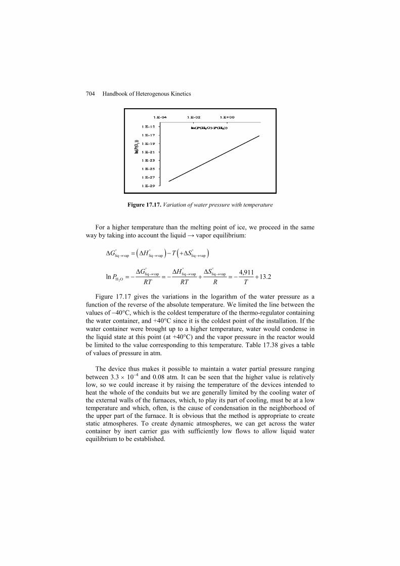
Figure 17.17. Variation of water pressure with temperature

For a higher temperature than the melting point of ice, we proceed in the same way by taking into account the liquid → vapor equilibrium:

( ) ( )liq vap liq vap liq vapG H T S° ° °→ → →Δ = Δ − +Δ

2

liq vap liq vap liq vapH O

4,911ln 13.2G H S

PRT RT R T

° ° °→ → →Δ Δ Δ

= − = − + = − +

Figure 17.17 gives the variations in the logarithm of the water pressure as a function of the reverse of the absolute temperature. We limited the line between the values of −40°C, which is the coldest temperature of the thermo-regulator containing the water container, and +40°C since it is the coldest point of the installation. If the water container were brought up to a higher temperature, water would condense in the liquid state at this point (at +40°C) and the vapor pressure in the reactor would be limited to the value corresponding to this temperature. Table 17.38 gives a table of values of pressure in atm.

The device thus makes it possible to maintain a water partial pressure ranging between 3.3 × 10−4 and 0.08 atm. It can be seen that the higher value is relatively low, so we could increase it by raising the temperature of the devices intended to heat the whole of the conduits but we are generally limited by the cooling water of the external walls of the furnaces, which, to play its part of cooling, must be at a low temperature and which, often, is the cause of condensation in the neighborhood of the upper part of the furnace. It is obvious that the method is appropriate to create static atmospheres. To create dynamic atmospheres, we can get across the water container by inert carrier gas with sufficiently low flows to allow liquid water equilibrium to be established.


T (°C) T (K) °vapΔG Pvap (atm.)

−40 233 15,550 3.30 × 10−4

−30 243 14,385 8.09 × 10−4 −20 253 13,239 1.85 × 10−3 −10 263 12,094 3.96 × 10−3 0 273 10,949 8.04 × 10−3 10 283 9,853 1.52 × 10−2 20 293 8,758 2.75 × 10−2 30 303 7,663 4.78 × 10−2 40 313 6,568 8.02 × 10−2

Table 17.38. Vapor pressures between −40°C and +40°C

2. We can carry out the calculation and the reasoning on mixture CO/CO2, satisfying us to give the results and specificities for the mixture H2/H2O, which can be studied in the same manner.

The equilibrium is represented as follows:

2 21CO CO O2

= +

The application of the law of mass action gives:

2 2

2

2 2CO CO2

OCO CO

2exp T

P PGP K

P RT P

°⎛ ⎞ ⎛ ⎞⎛ ⎞Δ= = −⎜ ⎟ ⎜ ⎟⎜ ⎟

⎝ ⎠⎝ ⎠ ⎝ ⎠

which we can represent in the following form:

2

2

COO

CO

2ln 2lnPGP

RT P

° ⎛ ⎞Δ= + ⎜ ⎟

⎝ ⎠

From the thermodynamics data in Table 17.36, we can calculate the standard Gibbs energy change at T = 1,000 K as follows:

( 110,435 393,129) 1,000(197.71 0.5 204.82 213.43)

196,003 J/mole

G H T S

G

° ° °

°

Δ = Δ − Δ = − + −+ × −

Δ =


which provides the equation for the partial pressure of oxygen as follows:

2 2

2

CO COO

CO CO

2 196,003ln 2ln 47.14 2ln8,315 1,000

P PP

P P⎛ ⎞ ⎛ ⎞×

= − + = − +⎜ ⎟ ⎜ ⎟× ⎝ ⎠ ⎝ ⎠

Figure 17.18 gives the line obtained in the axis system ( 2

2

COO

CO

ln / lnP

PP

).

Figure 17.18. Oxygen pressure produced by the mixture CO/CO2 at 1,000 K

Table 17.39 gives a table for values between the boundaries 10−3 and 103 for the

ratio 2CO

CO

PP

.

It can be noted that the oxygen pressures so obtained are extremely low.

Table 17.39 also gives the results obtained for mixture H2O/H2. The pressure obeys the relationship:

2

2

2

H OO

H

ln 48.34 2lnP

PP

⎛ ⎞= − + ⎜ ⎟⎜ ⎟

⎝ ⎠

Taking into account the possible minimal and maximum values for water vapor and calculating as described previously (Table 17.37), the maximum ratio that is possible is 0.08/0.001 = 80.2 whereas the minimal ratio is 3.3 × 10−4.

On comparing the tables, we note initially that the pressures obtained are very low. In addition, such a device is useful for kinetic studies only if we ensure that


gases other than oxygen do not react with the sample. For example, in an oxidation of a metal, it is necessary to ensure that the water does not react directly with metal or that carbon dioxide does not produce carbonate with the oxide. Finally, these devices although give excellent results for obtaining very low pressures for thermodynamic studies, they are not generally useful for kinetic studies, yet the low pressures are interesting.

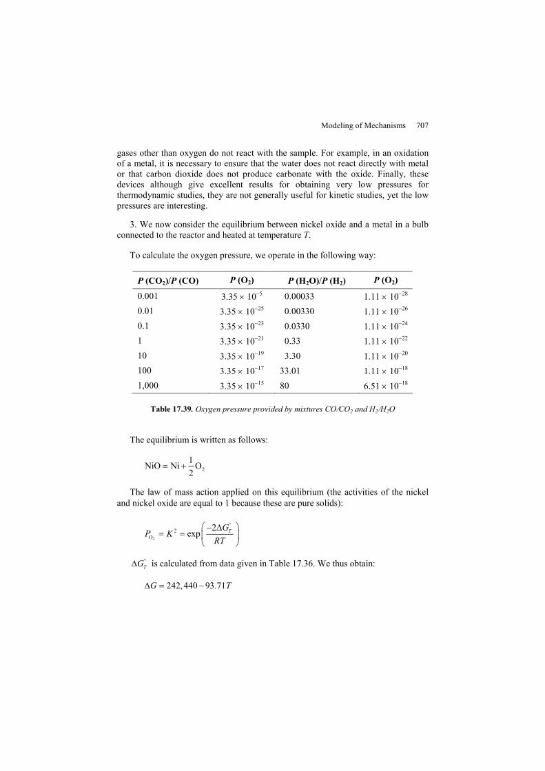
3. We now consider the equilibrium between nickel oxide and a metal in a bulb connected to the reactor and heated at temperature T.

To calculate the oxygen pressure, we operate in the following way:

P (CO2)/P (CO) P (O2) P (H2O)/P (H2) P (O2)

0.001 3.35 × 10−5 0.00033 1.11 × 10−28 0.01 3.35 × 10−25 0.00330 1.11 × 10−26 0.1 3.35 × 10−23 0.0330 1.11 × 10−24 1 3.35 × 10−21 0.33 1.11 × 10−22 10 3.35 × 10−19 3.30 1.11 × 10−20 100 3.35 × 10−17 33.01 1.11 × 10−18 1,000 3.35 × 10−15 80 6.51 × 10−18

Table 17.39. Oxygen pressure provided by mixtures CO/CO2 and H2/H2O

The equilibrium is written as follows:

21NiO Ni O2

= +

The law of mass action applied on this equilibrium (the activities of the nickel and nickel oxide are equal to 1 because these are pure solids):

2

2O

2exp TG

P KRT

°⎛ ⎞− Δ= = ⎜ ⎟

⎝ ⎠

TG°Δ is calculated from data given in Table 17.36. We thus obtain:

242,440 93.71G TΔ = −


and

2O58,314ln 22.54P

T= − +

Figure 17.19 gives the line of the preceding function in the axis system (ln P, 1/T) and Table 17.40 gives a series of numerical values. It is seen that the range of oxygen pressure is wider than with the gas mixtures. This method is especially interesting for experiments carried out at high temperatures because the studied sample must be at a higher temperature than the sample in the container in which the equilibrium is established (so as not to distil nickel from the container into the sample).

Figure 17.19. Pressure of dissociation of nickel oxide

T (K) 646 746 846 946 1,046 1,146 P (O2) 3.8 × 10−30 6.9 × 10−25 7.1 × 10−21 1.0 × 10−17 3.8 × 10−15 4.9 × 10−13

T (K) 1,246 1,346 1,446 1,546 1,646 P (O2) 2.9 × 10−11 9.4 × 10−10 1.9 × 10−8 2.6 × 10−7 2.5 × 10−6

Table 17.40. Oxygen pressures generated by the dissociation of NiO

handbook of heterogenous kinetics (soustelle/handbook of heterogenous kinetics) || modeling of...

Documents