Fermi National Accelerator Laboratory

FERMILAB-Chf-9l!275-E

Hadron Collider Physics

L. Pondrom

Physics Department, University of Wisconsin 1150 University Avenue, Madison, Wisconsin 53706

Oct0ber 1991

* A Series of Lectures presented at CINVESTAV, Mexico, D.F., July, 1991.

sled by UniverrlUes Research Assodatlon Inc. under cunlracl with the United Slaler DeparimeoI of Energy

CDF/PUB/CDF/PIJBLIC/l586 FERMILAB-CONF-91/275-E October 3, 1991

HADRON COLLIDER PHYSICS

A Series of Lectures given by

LEE G. PONDROM Physics Department, University of Wisconsin,

1150 University Avenume Madison, Wisconsin 53706, USA

at

CINVESTAV, Mexico, D.F. July, 1991

ABSTRACT An introduction to the techniques of analysis of hadron collider events is

presented in the context of the quark-parton model. Production and decay of W and 2 intermediate vector bosom are used as examples. The structure of the Electroweak theory is outlined. Three simple FORTRAN programs are introduced, to illustrate Monte Carlo calculation techniques.

Introduction

These lectures are intended for a classroom rather than a technical seminar. A review of the present experimental situation in hadron collider physics has been pub- lished elsewhere? Here we will attempt to explain the ideas behind the interpretation of hadron collider events. To do this we rely heavily on some standard texts in the field: “Collider Physics” by Barger and Phillips;* “Quarks and Leptons” by Halzen and Martin;3 “Gauge Theories of the Strong, Weak, and Electromagnetic Interac- tions” bye Quigg;4 “Gauge Theories in Particle Physics” by Aitchison and Hey;s and “Concepts of Particle Physics” by Gottfried and Weisskopf.6 The periodic publications of the Particle Data Group7 furnish the latest experimental results and in addition establish conventions to be followed in defining parameters of the theory, naming the particles, etc.

In the notes that follow we will borrow freely from these texts, sometimes citing specific sources, but sometimes not.. We admit our debt to the above authors at the outset, hoping that lapses in citation will henceforth be forgiven.

The selection of topics and the organization has been chosen to cover the subject in five one hour lectures. Although much material has been omitted by necessity, the objective of these notes is to be comprehensible and self contained.

There are homework problems scattered throughout the notes, which should be worked out by the interested reader. Calculating physical quantities is always en- lightening, and is necessary for progress to be made in the science.

1

Lecture I

1.1 e+e- Annihilation

Quantum electrodynamics is a good place to start. The interactions of charged leptons and photons can be accurately described by the Feynman rules. These rules have been extended to cover the Electroweak theory and QCD as well, so the more familiar QED furnishes a natural framework to introduce the notation and kinematics.

We begin with the four dimensional notation for photons and leptons, the Dirac equation, and the application of the Feynman rules to the calculation of cross sections. All of the texts mentioned above have adopted the four dimensional metric tensor defined by Bjorken and Drell?

(1.1)

so that the space components of a lower index four vector have the opposite signs to those of an upper index four vector:

x0 = {x0,5}, xp = {x0, -5) X&@ = t* - 52 (1.2)

We will adopt natural units throughout: h. = c = 1. In these units length, time, and l/energy have the same dimensions. For cross sections, (1 GeV)-* = 0.389 mb is handy, while for decay rates fi = 6.58 x lo-r5 GeV-set does the trick. There is no distinction among the uni$ for mass. momentum, and energy.

The gradient 8, = G transforms like a lower index vector. A simple Lorentz

transformation to a prime frame moving with velocity +v along the 3 axis is

xv’ = air’ with ai = and y = (1.3)

The Dirac equation in momentum space in this metric for a free positive energy electron reads

(k - mbb) = 0, i? = YP,. (1.4)

In coordinate space the form is (iy”8, - m)$(z) = 0, with p, = ia,. The adjoint equation is

G(p)& - m) = 0. (1.5)

where ii = uty’ and yp’ = y”y’y’.

The corresponding negative energy spinor equations are

(h+m)v(p) = 0, and C(p)(k + m) = 0. (1.6)

The anticommutator of the g-a matrices is

y'l7"+7"7# = 2g'Y. (1.7)

Invariant variables first introduced by Mandelstam are very useful for describing the kinematics of reactions of the type A + B + C + D. QED formulas exhibit useful symmetries when written as functions of these variables. In terms of the four momenta of the particles, they are defined as follows:

s = (PA + PB)'

t = (PA - PCj2

u = (PA - PD)* (1.8)

with the constraint s + t + u = mi + m& + rng + m;. The rapidity of a particle is defined relative to the direction of motion of the AB rest frame bv the loga~th~c

relation: y=iln E

( ) E - Pll (1.9)

Rapidities add algebraically when going from one Lorentz frame to another, as long as the motion is parallel to the original AB direction. Therefore rapidity differences, or shapes of rapidity distributions. are invariant under such Lorentz transformations. The maximum value of the rapidity for a particle of mass m in a system with total energy 6 is

d ymar=ln - ( ) m

(1.10)

Since at high energies the particle mass can be neglected, the pseudorapidity is often

n=iln(~~~~S~) =-ln(,,i) (1.11)

Psuedorapidity depends only on the polar angle. This definition is invalid for very small angles where the quantity in Eq (1.11) is larger than the allowed maximum of Eq (1.10). At the SPS and Tevatron colliders, pseudorapidity is never a good approx- imation for W and 2 bosons. They are too heavy, and so is the as yet undiscovered top quark. But it works well for everything else. Because of the invariance of rapidity differences, many detectors are segmented in constant bites in An.

In order to perform calculations. we must know how to relate cross sections and decay rates to invariant matrix elements, which in turn are calculated from the Feyn- man rules. The decay rate formula will be introduced in Lecture III. The differential

3

cross section per unit solid angle for the process A + B -+ C + D in the AB rest frame is given bv the formula

do ~=&f;IM12

. where M is the invariant matrix element for the reaction, and s = (pa + p~)~ is the

Mandelstam variable.

v;;Hc, u(3---&q 42 EPC)

Figure 1.1. Feynman rules for t?+e- + p+p-.

Figure 1.2. Compton scattering diagram and Feynman rules.

Figure 1.1 shows the Feynman rules applied to the basic reaction e+e- + p+p-. The invariant matrix element can be written down by applying the factors shown in the Fig.-the spinors, the vertex factors, and the photon propagator-as follows:

- iM = iei&)y”u(pA) 7 ieG(pc)-/‘t~(p~) (‘)

(1.13)

where s = qz = (mass)2 of the intermediate photon. The Compton scattering diagram involves real photons and an electron propagator, as shown in Fig. 1.2. In this case the photon is characterized by a four momentum and a polarization four vector. Similar formulas will be obtained for real W’s and Z’s The use of the Feynman rules in this case gives the amplitude:

- iM = ii +ey i(kA + ;F + m)

(PA + ky _ ,zZe-fYtu ‘(?‘A) 1

(1.14)

The amplitude for the crossed diagram must be added coherently to Eq (1.14) to obtain the correct expression for the cross section.

The annihilation process e+e- + p+p- IS of fundamental importance in electron storage rings. In the high energy limit where all of the lepton masses can be ignored, the differential cross section is

do 02 t2 +u2 zi=2s 32

(-) = ;(I fcossB), (1.15)

e* 1 where o = - = -. The total cross section is:

47r 137

4

HOMEWORK PROBLEM: Use the Feynman rules to derive the differential and total cross sections for e+e- -+ ,u’p-, Eqs. 1.15 and 1.16 above. To perform the spin sums, use the trace theorems given in References 3 and 4. Note that the trace factors into two terms which have the same form. The Mandlestam variables of Eq. 1.8 have been simplified by the zero mass approximation.

1.2 The Standard Model

The standard model is built with six leptons and six quarks (and their antipar- ticles) given in Table 1. The quark varieties are called flavors, and each flavor comes in three colors. There are four gauge fields: y, 2, and W of the electroweak sector, and 9 for QCD. The photon and gluon are massless, while the 2 and W are very heavy. There are eight gluons carrying the colors of the 3 x 3’ octet representation of color SU(3). Leptons are restricted to electroweak interactions. The quarks share the electroweak forces, and in addition couple to gluons through the color charge to give QCD. Neutrinos are assumed to be massless. In fact, at ,/Z Z 1 TeV all leptons and quarks except for the t and perhaps the b may be considered massless.

Table 1: “Standard Model” Ingredients

Leptons Charge Quarks Charge ve VI1 VT 0 11 c t +$

e- p- T- -1 dsb -5

A quark-antiquark pair can be produced instead of a lepton pair in the final state after efe- annihilation. The cross section for this process in its simplest form is just like Eq. 1.16, weighted by the square of the quark charge and multiplied by 3 for color, which gives a formula for the ratio R:

R= o(e+e- -+ q@)

f7(e+e- + p-p+) =3x&;.

f (1.17)

R = 2 below charm threshold; R = 3; between charm and bottom thresholds; and R = 3: above bottom threshold. The top quark threshold would cause a step in R of 1; units. There are QCD corrections to these numbers, and in the resonance regions near the J/T), upsilons, and 2 there is sharp structure in the ratio, but the trend in R, shown in Fig. 1.3 (Ref. 7), foil ows expectations. The lower part of Fig. 1.3 shows R above the upsilon region. where a search has been made for the top quark threshold to no avail. The rise above 50 GeV is due to the tail of the 2 pole, which is centered at (91.161 f 0.031) GeV!

5

5; yam 1, *

,‘r I;, i ‘II ‘1 / /,

: I : i ~,~l!,,‘:“l!i’fi~‘~~~“~l~.~ 1 ./I

/

3E ,i

p+,,, I !’ I$(~,

1

1

3 ’ 1 2 4 6

s-

: : Dun 51&D*

3Tr:“s, :Zf *mu .E ;

;& ~can?usAlt:~‘ xs:, ~nwrO .mmn

2 :0 20 20 i; 50 60 I.. !&“I

Figure 1.3. R = (e+e- - hadrons)/(e+e- - p+p-)

The Electroweak theory specifies how the 2 propagator and the photon propa- gator interfere. The formula for the cross section obtained by the coherent sum of amplitudes for these two intermediate states

e+e- + qq= w + >--T--< 2

charge Q/

is given by

da - = g [4??(1 t dR

~0s’ 8) - 2Q,x1{ VV,( 1 t cos’ 6’) - 2a, cos 6’)

tX2{(V,?+a~)(l t Vz)(1+cos2fJ) -SVV,a~cosB)] (1.18)

The first term is the same as Eq. 1.15. The second term, involving the real part of the Breit-Wigner amplitude ~1, is the interference between the photon and the 2. Here the vector-vector interference is symmetric, while the vector-axial vector part is linear in cos 0, the angle between the electron and the outgoing fermion, and results in a front-back asymmetry. The third term, multiplied by the square of the Breit-Wigner amplitude x2, is the 2 amplitude squared. Here the vector and axial vector parts of the 2 coupling to fermions contribute to the (1 $ cos* 0) term, while the vector-axial vector interference of the 2 itself gives an asymmetric part. As we shall see, the 2 coupling is almost pure axial vector, so the x2 asymmetric term is small. The yr term can be large, but it changes sign as the energy increases through the 2 pole, and vanishes on resonance. The variation of the coefficient of cos0 as

6

the energy passes through the 2 resonance is shown in Fig. 1.4. These properties are clear from the formulas below:

0.5

‘: y 0.0 L&u

~0.5

1

xl = s(s -l@)

16sin’Ow co9 Ow (s - M:)* + rz~; 1 s=

X2 = 256 sin4 0~ co& Bw (s - Mj?)? + PM;

V = -1+4sin*Bw (leptonic vector term)

af = 2T3, (at = -1)

VI = 2T3, - 4Qr sins&; T3 = +t for ue,ulrru,c,t

-; for e-,p-,r-,d,s,b (1.23)

/

/ /

‘L, \ 11,,,/~1,,,,,/,,,,,,,,,,,, 70 so 90 100 110 120

E 4.”

L

Figure 1.4. Asymmetry of e+e- - ,u+p- as a function of energy.

40, 1 : 35 F ~ / ob!or* i, 3

1 ;

30 t E

+i,, : :::;:, q

zsi o ,I, ’

-

.!I 1, I

z i *OPAL 2 ZOf ; . ,,?I Y

3 !i 7 ,a 80 ,.. lop &.

r --3 us - ig ----airs ‘,‘&+ 2 2 7 0; 88 99 90 91 92 33 94 ‘?j

\s i i;, ,ct’.‘,

Figure 1.5. Z resonance line shape

In the following lectures we will attempt to justify these assignments. The Wein- berg angle 6w is a parameter of the theory. The first measurements of 0~ were performed by studying the neutral current cross sections in neutrino scattering, with the result sins Bw = 0.23, which results in a vector coupling constant for leptons of 0.08, about 10% of the axial vector coupling.

Figure 1.5 (Ref. 7) shows the cross section for e+e- annihilation into hadronic final states--i.e., alI quark final states which then dress themselves into jets of hadrons-as the energy is varied through the 2 resonance. The plot shows the consistency of the cross section data with the hypothesis of three neutrino families, and gives reality to the above formulas characterizing the 2 as a massive intermediate state. In the next lecture we will see how these formulas apply to hadron colliders.

7

Lecture II

2.1 The Drell-Yan Process in Hadmnic Collisions

In the quark-parton model, hadrons are assumed to consist of free point particles with negligible mass, dubbed partons by Feynman. These partons have been iden- tified as fractionally charged quarks and neutral gluons. This picture is valid in an impulse approximation: the hadron is probed for a very short time span, correspond- ing via the uncertainty principle to a very large energy transfer, during which only one parton participates in the reaction, and the other constituents of the hadron act as spectators. The incident projectile, which is a lepton in lepton-hadron collisions (deep inelastic scattering) and another parton in hadron-hadron collisions, strikes a parton which carries a momentum fraction 0 < z < 1 of the total momentum of the target. The collision occurs between point particles, analogous to e+e- annihilation, except that the kinematics are determined by zr and zs, while for e+e- zt = zs = 1. The probability distributions of parton momenta in the hadron are called structure functions? More will be said about them later.

Equation 1.18 for the process e+e- -+ @can be time reversed without any changes to describe the inverse reaction 44 -+ e+e-, which in the parton model is the sub- process for the observed reaction p + p + e+e- f X, and is called the Drell-Yan mechanism, shown in Fig 2.1. We proceed with the kinematics of the reaction in the pp rest frame, which coincides with the laboratory frame at the SPS and Tevatron colliders. The parton model differs from e+e- annihilation in two important ways:

a) the qq rest frame does not in general correspond to the pp rest frame, so that the lepton pair can be moving in the laboratory along the beam direction (Trans- verse motion also happens, but can be neglected in first approximation.); and

b) although the Fp system is neutral, the Qq system need not be, which permits the production of not only the 2 boson, but single W+ or W- as well. Production of Wf, at least until LEP 200 begins operation, is the sole province of hadron colliders.

The qq collision is collinear, with total momentum

and energy

p'g t & = i (2.1)

Eq t Eq = Ec, (2.2)

Now introduce the momentum fractions z1 and .rr:

& = 2, P. and $@ = ZZ( -F) (2.3)

8

where P and -P are the proton/antiproton incident momenta, and xl, .rs are dimen- sionless variables. Momentum conservation then gives the momentum fraction of the intermediate state (or the lepton pair) as

k=( 5, - z*)P or I = 51 - 52.

Since Ek = (x1 + ss)P, M2 = Ei - i* = 4z1z2P2, resulting in

(2.4)

2112 = M21s, (2.5)

where s = 4P*. The rapidity of the produced state y is given in terms of zr and x2 by

q,2 = $eiy I S I’ I”’ WI

‘03 B’?

t \ XUW 1

1’ \

Figure 2.1. Drell Yan mechanism in the Parton Model

3.4 ’ \ ,- / \rm

/’ 3.2 l;r::, 1

\ XlUI

O-O0 0.2 i4 Jy

‘L, ,,,-. _

0.6 0.8 +~‘

Figure 2.2. Field and &nnan structure functions U, d, s for the proton.

The Dreh-Yan cross section for an intermediate photon, i.e. well below the Z resonance, can be written down from the definitions of the structure functions and the basic formula of Eq. 1.16. Thus

d2Gp --, e+e-,Y) = $$ C&~[q.(2,)q,(12)dlld~*] a

v-7)

where A@ is the square of the mass of the lepton pair, and Q. is the quark charge. The factor of l/3 is for color, because only color. neutral qq pairs are allowed in the sum, and the structure functions are identical for the three quark colors. For simplicity the quark is assumed to reside in the proton and the antiquark in the antiproton, although it is possible for the two to be reversed. Antiquarks occur in the proton only as vacuum fluctuations of qq pairs. The proton structure functions are u and d valence quarks, plus ZLu , dd, and Ss sea quarks. The gluons play no direct role in either deep inelastic scattering or the Drell-Yan mechanism-a reason why the gluon structure functions are not as well known as those of the quarks. Quark structure functions for the proton obtained by Field and Feynman’a are shown in Fig. 2.2.

9

With a change of variables Eq. 2.7 can be written in terms of dM* ds:

d% 4xa*

dM*dx = 9~2~~~2 f 4M2,s11,2 F Q:q.(~lka(d (2.8)

HOMEWORK PROBLEM: Show that this expression follows from Eq. 2.7,

2.2 The Structure Functions

Deep inelastic lepton scattering experiments (e’s, p’s, and Y’S) have been the sources for the structure functions: which are obtained by fits to the data. The structure functions cannot be derived from first principles, and must be calculated empirically. Examples of deep inelastic scattering in the parton model together with the kinematics are shown in Fig. 2.3. The cross section is linear in the structure functions (only one hadron), so by assuming charge conjugation invariance-u in the proton equals ri in the antiproton-the Drell-Yan cross section can be written down directly in terms of measured proton characteristics. This is the interpretation of Eq. 2.8. Unfortunately this procedure does not quite work, as the cross section so calculated is about 2/3 of the experimental value. To fix things up, a “I( factor” of 1.5 is applied to the right hand side of Eq. 2.8. This factor can be calculated in QCD.

q2 = t = (P.~ - pc)*; v = EA - EC z = -q*/2mpv > 0

Figure 2.3. Deep inelastic scattering in the parton model

The motion of bound nucleons in a spinless nucleus is spherically symmetrical, and related to the Fourier transform of a nucleon wave function. Do the quark structure functions in the proton arise from similar considerations? The answer is yes, but there is a fundamental difference between nucleons and nuclei.

Consider a nuclear analog of the proton with its three valence quarks (rr, u, d)- He3 (p, p, n). The negative binding energy of He3, about 6 MeV, is much smaller than the masses of the constituents. so we may safely write the mass formula for the nucleus as:

M=3m (2.9)

10

Now boost the nucleus to very high momentum:

P=7M=3yn (2.10)

Now each “parton” has l/3 the momentum of the nucleus, and hence I = l/3. The nucleon motion smears this delta function out a little bit, the width being equal to the nucleon motion in the transverse plane.

The proton is a very different object. We are told that the quarks are confined- they cannot escape as free particles-and that the quark masses are negligibly small. Hence a formula like Eq. 2.9 is not valid. Hadrons, unlike any other materials, weigh more than the sum of their constituent masses. Nothing else does this - atoms, nuclei, lead bricks, etc all weigh less than their parts. The energy which forms the proton mass in its rest frame is kinetic, so we write the analog of Eq. 2.9 as follows:

M = C Ei i

(2.11)

where E; is the kinetic (or total) energy of the massless ith constituent. To conserve momentum, there must be at least two partons, and the maximum value of A?, for any parton is

(&Lx = M/2 (2.12)

Now boost the hadron to high momentum by multiplying both sides of Eq. 2.11 by the Lorentz factor:

Since Cipiil = 0 in the proton rest frame, it can be added to the right hand side of Eq. 2.13 without penalty:

P = YC(E +pill) (2.14)

The longitudinal momentum of the ith parton in the boosted frame is Pi = Y(Ei+pill),

and the momentum fraction I = p, where both terms are proton rest frame quantities. Note that since E,, = pllmax = M/2, and plf can be plus or minus, the range for z is 0 < z < 1. This is Feynman’s I. The Lorentz invariant transverse momentum can be ignored.

Thus confined massless partons are the key to understanding the structure func- tions. The binding of the partons and the fact that the number of partons is not fixed play a role, in fact it is the binding that gives the shape of the I distribution, but these considerations are not fundamental to obtaining a momentum fraction anywhere between zero and one. Free massless particles will do that very nicely. If we knew how to solve the Dirac equation and obtain wave functions for the bound massless partons, then their distributions in momentum space would permit the calculation of u(z). So far we are not able to solve this bound state problem?’

11

,?.3 Hadronic Z production

The Drell-Yan formula Eq. 2.7 can be readily adopted to the case where the intermediate photon and Z interfere. Equation (1.18) when integrated over the solid angle gives the cross section for 4. + Q,, -+ e+f?X as:

- 2QaVKx1+ (v,2 + a:)(1 + v*)~~] (2.15)

where S is the square of the mass of the lepton pair, Q. is the quark charge, and (V,,a,) are the vector and axial vector coupling coefficients for the quarks. The Z Breit-Wigner terms are xr and ~2. The details are given in Eqs. 1.19-1.23. It follows then that in the parton model the cross section for pp + e+e-X is given by (neglecting the sea quark contributions):

Po(fip + e+e-x) = taa2 K 3p-j- ~[Q~-2Q.Vv,x~+(V~+~~)(l+V2)x,],(~,)~~(rz)dz~dr2. (2.16)

On resonance S = i$$, the Qz term is negligible and the x1 term vanishes, so that

V,’ + a:)(1 + V2)xzqy(ll)9,(22)dsld12 (2.17)

The variables can be changed to rapidity and M* by using the identity dzldsz = dydM’/s, where s refers to the pp system. The result is

v,’ + d)(l + V2)X*Qohka(+2) (2.18)

Integrating over the Breit-Wigner and using the partial width formula T(Z -+ e+!-) = GF@(I + I’*)

241,&r grves the result

do -=----L dy

r,f, Gd&tw2 [(I - $w t 3&)451)4x2) + (1 - T&v t $z$)d(z,)d(~,)] (2.19)

where sin* 0 = zw, and & = I?&. Here we have introduced the Fermi coupling constant GF, the characteristic strength of the weak interactions, which is derived from the muon lifetime. This agrees with the equation on p. 252 of Ref. 2.

HOMEWORK PROBLEM: Derive Eq 2.19 from Eq 2.18. Hint:

J idi ~Mz o (i -&if;)* + PM; = 7

12

Lecture III

3.1 Hadronic W Production

In the last lecture we learned that the hadronic reaction to produce a high mass lepton pair, pp -+ !+f-X, proceeds via the parton model through the subprocess qq -t e+t!-, which is the inverse of the e+e- annihilation into qq (two jets).

Since the 44 pair can have a net charge, single W’s can also be produced in pp collisions by an extension of the Drell- Yan mechanism to include weak charged currents. The analog to Eq. 2.19 for pp -t W+X -+ efvX is:

$(pp + w+ + e+v) = ~~Br.I(lizzu(ll)d(lZ). (3.1)

BC, = Ply/F is the branching ratio for the decay of the W into a (!, v) lepton pair. Eq. 3.1 produces a W+ by the simplest parton model process: a u quark in the proton annihilates a d quark in the antiproton to produce a W+ plus spectator debris. In a similar fashion a W- would be created by the annihilation of a d in the proton and a ii in the antiproton. This model gives similar interpretations for neutral lepton pair (e+, e-) and charged lepton pair (e*, U) production in fip collisions.

The missing neutrino in W* decay complicates the reconstruction of the events in the laboratory. The transverse momentum of the neutrino can be inferred from measured quantities and momentum conservation, but the longitudinal momentum is unknown. In principle pll could be determined by conserving momentum in the beam direction, but it is usually not possible to do this because measurements cannot be made close to the direction of the colliding beams. As a result, there are two solutions for cos0 the polar angle of the charged lepton in the W rest frame. Transverse momentum balance gives:

-M& sin2 e $4 = -6~. , or 7%~ IL = 4

Hence the two solutions for cos 6’ are symmetric about 7r/2 in the W rest frame:

4PL ( ) l/2

cosf?=& l-- M&

(3.2)

These two values correspond to two W momenta in the laboratory. This is a kinematic ambiguity, characteristic of a zero constraint fit.

Figure 3.1 shows the W+ rapidity distribution calculated with the W-PROD pro- gram described in the APPENDIX for ,,6 = 1800 GeV (the Tevatron). Eq. 3.1 and the simple structure functions of Feynman and Field were used for these calculations. Figure 3.2 shows the charged lepton rapidity distribution, which, in contrast to that

13

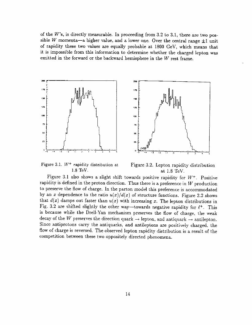
of the W’s, is directly measurable. In proceeding from 3.2 to 3.1, there are two pos- sible W momenta-a higher value, and a lower one. Over the central range fl unit of rapidity these two values are equally probable at 1800 GeV, which means that it is impossible from this information to determine whether the charged lepton was emitted in the forward or the backward hemisphere in the W rest frame.

Figure 3.1. Wf rapidity distribution at Figure 3.2. Lepton rapidity distribution 1.8 TeV. at 1.8 TeV.

Figure 3.1 also shows a slight shift towards positive rapidity for W+. Positive rapidity is defined in the proton direction. Thus there is a preference in W production to preserve the flow of charge. In the parton model this preference is accommodated by an I dependence to the ratio u(z)/d( ) f t I o s ructure functions. Figure 2.2 shows that d(z) damps out faster than u(z) with increasing I. The lepton distributions in Fig. 3.2 are shifted slightly the other way-towards negative rapidity for e+. This is because while the Drell-Yan mechanism preserves the flow of charge, the weak decay of the W preserves the direction quark + lepton, and antiquark -+ antilepton. Since antiprotons carry the antiquarks, and antileptons are positively charged, the flow of charge is reversed. The observed lepton rapidity distribution is a result of the competition between these two oppositely directed phenomena.

14

$1” = -P;jet - P;f Q=P+P’

Figure 3.3. Vectors in the transverse Figure 3.4. Feynman rules for plane for Mf u+d+ W+i?+u.

3.2 The Transverse Mass

The kinematic ambiguity resulting from a zero constraint fit to W decay assumes that the W mass is known. If measurement of the W mass is the experimental objective, then one constraint goes away, and the events are no longer reconstructable. It is possible, however, to work with transverse variables. and define a transverse mass by the equation:

M: = 2PClP,l(l - cm 4b) (3.4)

where the measured and inferred vectors in the transverse plane are shown in Fig. 3.3. From the definition it is apparent that the maximum value of Ml is the true mass. There is another transverse mass sometimes used in kinematics, defined by the formula rn: = m2 + p:, which has a minimum value of the true mass. Do not confuse the two.

Equation 3.1 is the cross section per unit rapidity times the branching ratio, integrated over angles and over the Breit-Wigner formula for the W line width. We can now derive this relation from first principles, following the procedures of Lecture II for the 2 production and decay, and borrowing the matrix element from muon decay given by Eq. 3.20 below. The Feynman rules for the reaction u + d -+ !+ + v are shown in Fig. 3.4 The matrix element for this reaction is given by:

,(/f = s2(WW(l - 75)4P)+,(qr (1 _ y5)u(k)), 8 i--M&+iM~r p (3.5)

15

In writing down Eq. 3.5 we have added an imaginary term to the propagator to account for the line width of the W. The momentum terms in the numerator of the propagator do not contribute because of the Dirac equation. If the dimensionless constant g* and the Fermi constant GF are related by

-=- (3.6)

then in the low energy limit 3 < M& E q. 3.5 has the same form as Eq. 3.20. If we substitute g*/8 = GFAI$/J~ into Eq. 3.5, introduce the Mandelstam variables .? = (p + p’ )’ and C = (p - k)*, and evaluate c IMI*, we get the result:

srhn

c lMI* = 64 spins

(3.7)

Dividing by four to average over the u and d quark spins (the wrong helicities do not contribute to the cross section), and using the cross section formula Eq. 1.12 gives the expression

dc? 1 GFM$

4 )

2

%=i = 16x2 q 1 - cos 0)’

fi (i - M&)2 + M&P (3.8)

Here the angular distribution factor (1 - cos O)*, mentioned above in the discussion of the asymmetry in lepton rapidity, follows from the helicity rules. The cross section for pp, in terms of the structure functions, the K factor, and the l/3 for color is

du K

c-E=3 (3.9)

The differential cross section per unit W rapidity per unit solid angle can be obtained

from this expression by substituting the Jacobian dxldsz = dye. The result is: s

(3.10)

where the structure functions are evaluated at x1,* = (I”’ f .3

efy, The integration

over the Breit Wigner line shape then gives the cross section

da K GF -- - = 48. a dydfl i;wz+++2)(1 - ~0~4~. (3.11)

Finally, integration over the solid angle produces Eq. 3.1

16

HOMEWORK PROBLEM: Go through the steps from Eq. 3.7 to Eq. 3.11, and then to Eq. 3.1. You will need the W partial width into eu:

1 GFI~$ qw + ev) = - 6* & (3.12)

The derivation of Eq. 3.7 will be sketched below in the section on muon decay.

The angular distribution Eq. 3.10 can be transformed into an expression in terms

of transverse mass. Using M* - 4 * &. I - p,, and pl = -smB grves the Jacobian of this

transformation 2

dcOsB= p& (3.13)

This relation exhibits a singularity in the denominator for A4: = i, which is called the Jacobian peak. Although the distribution is singular, the integral is well behaved. The term linear in cos 8 in the angular distribution (1 - cos 0)’ averages to zero in the transverse mass expression, because the transverse variables are independent of the sign of cos 8. The transformed formula then becomes

i(l - cosB)‘dcosB = 2 - ws dhf2,

&xi@ L (3.14)

This derivation follows the discussion on pages 259 and 260 of Ref. 2. Equation 3.14 can be substituted into Eq. 3.10 to give the transverse mass distribution smeared by the Breit-Wigner line shape. Since the transverse mass does not depend on the rapidity of the lV, the expression can be evaluated at y = 0. In addition, as the energy is varied over the W line width, the structure fuctions u(z) and d(z) can be assumed constant in first approximation. The results of a Monte Carlo calculation based on these assumptions are shown in Fig. 3.5. The sharp peak at Ml = Mw comes from the denominator in Eq. 3.13. The program which produced this curve is described in the .APPE,NDIX.

17

Figure 3.5. Transverse mass distribution Figure 3.6. Transverse mass distributions for for the perfect detector. CDF data.

Experimental distributions for the W transverse mass are dominated by detector resolutions, which broaden the Jacobian peak considerably. The published results of CDF (12) are reproduced in Fig. 3.6. A cut on the lepton pi > 25 GeV has been made on these data to reduce low Ml background. The smearing of the curve is well described by modelling the detector response, as is apparent from the agreement obtained between the data and the expected shape. Very little sensitivity to the W line width remains in the measured leading edge. The W line width has been measured by an indirect method ?3 In this paper the cross section times branching ratio g(ji + p -+ CI/* + X)B( W -+ e*y) was divided by the corresponding expression for Z’s: cr(p + p + Z + X)B(Z -+ e+e-). The cross section ratio, believed to be less sensitive to theoretical uncertainties than either cross section alone, was calculated from the standard model. Then using the standard model for the partial width l?(W + ev), and the direct measurements of B(Z + e+e-) from LEP and SLC gave the value F = (2.19 +I 0.2) GeV, in agreement with expectations.

3.3 Quark Decays of W’s

The inverse of W production by qq is the decay of the W into quarks: CV+ -+ u + 2. According to the standard model 64% of all W’s decay this way. The leptonic channels W + ev and W + pv represent about 22% of W decays, so the detection of the qq final state would be beneficial for two reasons: a) it would increase the detection efficiency by a factor of 3; and b) it would give a constrained fit to the Ck’

18

mass, since there is no missing energy. Unfortunately, although the @J pair is color neutral, the individual quarks are not,

and are prohibited from appearing as free particles by confinement. As the quarks separate, the color field creates ijq pairs, which combine to form color singlet mesons (and qqq triplets which form baryons a few percent of the time). These mesons ap- pear in the laboratory as jets of particles. This process, which is called fragmentation, cannot be derived from first principles, but rather must be described phenomenolog- ically. Two approaches have been successful: the independent fragmentation model of Feynman and Fieldi4; and the correlated string model of the Lund group?5 The descriptions of the jets of particles are very similar in the two models. When there are differences between the predictions, the experimental data favor the Lund model.

Fragmentation models are based on extensive empirical data regarding the pro- duction of hadrons. It has been known for a long time that, as s increases, the mean transverse momentum (pl) remains roughly constant, and the average number of charged particles (n) increases only logarithmically with s. Thus the extra energy goes neither into more particles, nor into more pl. These observations lead naturally to the introduction of the scaling variable z = 2pll/&, or the related variable y of Eq. 1.9, and the expression of the cross section for hadron production as a Gaussian in pl times a function of y. In fact, the y dependence is almost constant, as can be seen from the logarithmic dependence of the multiplicity. Since the end points in rapidity increase logarithmically with s (Eq. l.lO), the multiplicity grows like log(s) if dn/dy is a constant. In this very simplified picture the multiplicity per unit rapidity is energy independent-like teeth in a comb. The length of the comb increases like

l%(S). The physical characteristics of a jet-its multiplicity, average pl, cone size. etc.-

depend upon the transverse energy of the jet. Longitudinal motions arising from the structure functions have no effect. The definition of a jet in terms of (An,&%) is independent of the polar angle. See Fig. 3.7.

Figure 3.7. Two jets with same ET but different thetas

In the APPENDIX a program which generates jets using the simpler technique of Ref. 14 is outlined. and some of the results are shown.

The fragmentation process greatly complicates the experimental task of identifying the W + qq decay for two reasons: a ) Quark fragmentation to produce jets is not

19

perfectly understood; and b) The response of a detector to jet energy is not very good. These effects combine to give a rather poor mass resolution in the expression

MZ = (EI + J%)* - (p; + p;)” (3.15)

where one and two refer to the jets. Resolution smearing results in a poor signal to noise ratio, where the noise comes from a continuum of QCD dijet events. The UA2 group at CERN has studied the dijet mass range from 50 to 130 GeV in search for an enhancement in the W/Z mass region?’ (The 2 is 11 GeV heavier than the W, but the mass resolution is unable to split the line.) The resulting distribution is shown in Fig. 3.8, and the background subtracted signal is shown in Fig. 3.9.

There are lots of jets in hadronic reactions, but very few line sources, which is one reason for the interest in these results. Another reason is that W’s and Z’s are expected to be signatures of new physics beyond the standard model, and so the detection of W’s with good efficiency through a kinematically constrained channel is important for the future.

I

28oor 4 -,r

I I 1 I k ' 1

60 80 100 I20 m,, (GW

Figure 3.8. WA2 jet-jet mass between 50 and 130 GeV.

Figure 3.9. Data from 3.7 after background subtraction.

There is one complication in the quark coupling, which we have ignored in Eq. 3.1. Namely, the flavor eigenstates (u.d) and ( c,s are not the states that couple at ) the weak vertex. This mixing phenomenon was first noted by Cabibbo before the c quark was discovered. Cabibbo introduced a mixing angle 8, and wrote the weak current (in modern notation) as

I I

600 c

0 /Y 1 T -“-

-zoo/+ 1

w 120 ml, IGNI

J’= (c ,)Y”(12-:5)GI ( ;)

where the mixing matrix U is

fJ= (

cos 8, sin 8, - sin 19, cos tic )

20

(3.17)

Experimentally sin8, = 0.22. All f o our amplitudes involving W’s coupling to u and d quarks should be multiplied by cos BC = 0.975. This idea has been extended to six quarks and a 3 x 3 unitary mixing matrix by Kobayashi and Maskawa.

3.4 Weak Interactions

We now turn to the phenomenology of leptonic weak interactions in the pre W/Z era. We want to show how particle decays and neutrino interactions can be described by a point four fermion interaction without an intermediate bosom how the divergence of the neutrino cross section with increasing energy can be avoided by the introduction of W* of unknown (but large) mass; and how the neutral current weak interactions were first observed in neutrino scattering. Then later we will learn that the standard model of Weinberg and Salam is able to predict the masses of the W and 2 bosons in terms of the Fermi coupling constant G F, the fine structure constant a, and the Weinberg angle 8w obtained from the strength of the weak neutral current. But first we need to review the traditional theory of weak interactions.

The decay rate formula in terms of the invariant matrix element, the companion to the cross section Eq. 1.12 describes the decay A +l+2+3+...+nisasfollows:

(2y;$E (2x)‘Q@‘(PA -P* -p* -. .P”) (3.18) (2~)~2E, (27~)~2& n

This is Eq. 4.36 in Reference 3. To describe the matrix element for muon decay via the Feynman rules, define the momenta

and the matrix element

p- i e- 0, Yir

p --t p’+k+k’ (3.19)

M = $ [GW‘U -Y%(P)] [4~‘)7,(1 - -r%(k’)]

This can be expressed as the dot product of two four dimensional currents:

In our metric, the parity violating operator y5 = i-y”7’7*y3, and has these properties:

7 5t = 75; (7”y = 1; 7’75 $-f-y’ = 0. (3.22)

Left handed and right handed spinors are defined by the following projection opera- tors:

i(l - 7s)u = UL; i(l + 7s)u = un. (3.23)

21

Evaluation of Eq. 3.18 for this decay gives the energy distribution of electrons as a function of E = E/E,,,, = 2p’/m,:

dI- G;m:, 2 - = y$r-pe (3 - 2E) de

(3.24)

The integral of this expression from zero to one gives the total decay rate, or the reciprocal of the muon lifetime, as

G;m; _ I q/L- + e-&v,) = - - -

1927rs rg

This is a very useful formula. It describes the decay of any spin l/2 fermion into three massless spin l/2 fermions.

HOMEWORK PROBLEM: Derive the formula Eq. 3.25 by evaluating the &, jMIZ and integrating over the phase space. Hint: The Capins factors into the contraction of two tensors which have the same form. Drop the final lepton mass terms. Check your intermediate result with Eq. 12.35 in Ref. 3:

; sg IM I2 = 64%~ k’)(k P’)

This equation is handy for working out the W production problem started in Eq. 3.5.

Equation 3.25 defines the Fermi coupling constant GF. The numbers are tabulated in Ref. 7:

mLl = 0.105658387 (34) GeV

l/T, = (0.455160 (8)) x 10s set-’

= (2.99592 (5)) x 10-i GeV (3.27)

which combine to give GF = (1.16380 (2)) x 1O-5 GeV-‘. This number differs by 2/1000 from the Fermi constant quoted in Ref. 7:

GF = (1.16637 (2)) x 10-s GeV-*. (3.28)

The difference arises from two small corrections to the muon decay rate: a) a phase space term of about 2/10000 due to the finite electron mass; and b) radiative cor- rections which alter the electron energy distribution, and when integrated affect the rate by 4.2/1000, and hence GF by half as much. The details of these calculations are discussed by Marshak. Riazuddin. and Ryan!7

22

Lecture IV

4.1 Neuttino Scattering

In his Nobel address Mel Schwartz ls described how the idea of attempting an experiment with high energy neutrinos came about. T.D. Lee raised the question at a coffee hour at Columbia: How does one study the weak interaction at high energy? Various ideas involving weak interactions of hadrons and charged leptons were raised and discarded, because of the unfavorable signal to noise. Neutrinos seemed the best choice to Schwartz, since they had only weak interactions. If enough neutrinos could be produced, and if backgrounds from other sources could be suppressed, then the signal in a massive detector would be observable, the signal to noise ratio would be tolerable, and T.D. Lee’s question could be answered.

Since the principal sources of high energy neutrinos are pi and K decays, muon neutrinos predominate over electron neutrinos in the beams. A typical beam has a few percent electron neutrinos. The neutrino/antineutrino ratio can be changed by charge selecting the pions and kaons. The basic reactions have the form vu + d + p- + u, or the conjugate ‘/,, + u -+ pt + d. The Feynman diagram, shown in Fig 4.la , is similar to beta decay. The matrix element for the process is:

M = 3 (G+Y’(~ -Y%(P)) (~(dh,(l - r”)u(k))

The sum over spins leads to an isotropic subprocess:

; c IM/* = 64G;(k .p)(k’ p’) = 16G$* SPW

(4.2)

Note the similarity to Eq. 3.26. The factor of l/2 is for the quark spin-the vP has only one spin state. Then the cross section in the (v,, d) rest frame according to Eq. 1.12 is

db(u,d --) /J-U) 1 dR

= $G$d and 6 = -G;;. iT (4.3)

The conjugate reaction can be readily calculated by substituting i for i in Eq. 4.2, which results in an angular dependence

g = $1 + cos8)2.

This can be understood by the heiicity rules, which forbid the (V,,u) reaction at 6’ = K, while (v,, d) has no problem reversing both fermion momenta. The total cross section is

&(F,u -+ P+d) = z. (4.5)

23

The subprocess i = IS , where + is the momentum fraction carried by the struck quark. If E, is the incident neutrino energy in the laboratory, and the target nucleon (N) is at rest, then s = 2M,E,. The ( v,,N) cross section depends of course on integrals over the structure functions, but the result is proportional to the incident neutrino energy. Experimentally

o(vp + N -+ ,a- +X) = 0.67 x 10mss cm* E,

and u(Vp + N + pt +X) = 0.34 x 1O-ss cm’ E,, (4.6)

where & is in GeV. The fact that the ratio of these numbers is two rather than three is a reflection

of the antiquark content of the nucleon. If the nucleon were made of three valence quarks, the ratio predicted by Eqs. 4.3 and 4.5 would obtain. See Section 12.8 of reference, 3 for more details.

The analogous purely leptonic reaction v,, + e- + v, + pL- has a very small cross section. Eq. 4.3 is correct, with S = s = 2m,E, at high energy, which gives the cross section

o(v,e- + v.p-) = 1.7 x 10e4i cm* E,. (4.7)

This is .0025 times the cross section of Eq. 4.6. The enhancement of the nucleon cross section is an example of quark binding and the structure functions. The masses of a u quark and an electron are not that much different, and yet the quark cross section is 400 times larger, because the quarks live inside a heavy object, so that MP rather than mp appears in the formula.

k %

p- k’ J’

x

y* w+

d u P

P, ..A+---“ Figure 4.la. Feynman diagram for Figure 4.lb. Same with Wft channel

u,+d-p-+u. exchange.

A cross section which increases linearly with E, cannot continue indefinitely, so there must be something wrong with the four fermion point interaction. (No roll over has been observed for neutrino energies up to 200 GeV.) It has been recognized for a long time that the introduction of a massive intermediate state as shown in Fig. 4.Ib would give a cross section which becomes a constant as s -+ co. Now we began these lectures with massive intermediate bosons. putting the cart before the horse from a historical standpoint. so the exchanged object in Fig. 4.lb is not big news. The vector boson propagator and the dimensionless vertex factors for charged

24

weak currents were introduced in Fig. 3.4, and used in Eqs. 3.5 ff. To summarize the structure. the vertex factor is

which corresponds to icy’ in QED. The matrix element for the neutrino reaction given by the diagram in Fig. 4.lb is then

,75)u(p) ,75)~(k) )) (4.9)

where the W propagator is

w,, = -i(gw + 9dYIwv) qz-M&

We know from Eq. 3.6 that, given GF, g and Mw are not independently specified. The standard model of Glashow, Weinberg, and Salami9 relates g to the electric charge e and the Weinberg angle Bw. This model, by combining electromagnetic and weak forces in the same scheme, requires the introduction of weak neutral currents.

4.2 Weak Neutral Currents

The discovery of weak neutral currents makes an interesting story, which has been reviewed by Galison. r” A brief description of the early history, and the influ- ence of what is now called the Standard Model on experimenters is given also by Steinberger. _ s’ Vuch of our knowledge of weak interactions comes from the study of decays of particles, but nature conspires in these decays to hide the weak neutral currents from view. For example, a neutral current decay like Co -+ AYV (u + uvv at the quark level) is energetically possible and violates no selection rules, but is swamped by the electromagnetic channel Co -+ Ay. Only flavor changing neutral currents like I(+ -+ atuP, which are forbidden by electromagnetic selection rules, are not overwhelmed. But alas flavor changing neutral currents are forbidden in first order by the GIM mechanism. ** So far no first order neutral current weak decays have been experimentally observed.

Weak neutral currents were discovered in neutrino reactions. Examples include elastic scattering like vLi + p + Ye + p, and v,, + e- + vP + e-, or inelastic scattering like v,, + p -+ v,, + X. These have all been observed and extensively studied. The cross section is not that small, being about 20% of the total neutrino cross section,

i.e., (4 -+ V”) (v, + p-1 + (VP -+ 4

= 0.2. One might ask why it took over ten years of

experimental work to find these effects ? This question is pursued in Ref. 20. In a nutshell, it was a combination of two factors:

25

4

b)

Until the early 1970’s, when the renormalization of the new theory had been proven, there was not a strong conviction that the weak neutral currents should really be there, and that the experimenters should search for them with vigor; and

Since neither the initial nor the final lepton can be observed, the signature of a neutral current reaction is a small amount of recoil energy, which can be lost in neutron background. Recent neutrino experiments have fine grained targets to observe the recoil energy, and employ timing and spatial distributions of events to discriminate against neutron background.

The neutral current vertex factor is written in terms of the Weinberg angle and the coupling constant g introduced in Fig. 3.4 and in Eq. 4.8:

-G yp w - ad) cos ew 4

(4.11)

where Vf and al were introduced in Eqs (1.22) and (1.23). The neutral current reaction

VW + e- --t VP + e- k i-p +k’+p’

can be described by extending the Feynman rules to cover 2 exchange, and writing the matrix element analog to Eq. 4.9:

- iM = ,c;;;, (+‘)y“(l -r5)4k)) Z,v (fi(~‘)-f(~ -;‘75)u(~)) (4.12)

where the Z propagator Z,,, is

z w

= 4%” + WY/G) q= - hf;

The matrix element can be simplified by approximating Z,, + igIIy/Mj in the low energy limit, by substituting cos* 6’~ = (M&/MS), a relation obtained in the standard model, and using Eq. 3.6 to eliminate Mw. The result is

iti = 5 (ii(k’)y,(l q+(k)) (~(p’)-f(~ -2af75)u(p)) (4.14)

Performing the average i CSpins IM 1’ and substituting into the cross section formula Eq. 1.12 leads to the total cross section for (~,,e) scattering:

o(v,e- + u,e-) = G;me& 27r

26

This equation involves the Weinberg angle in the vector coupling. The ratio of this cross section to its companion charged current cross section at the same neutrino energy is

a(v,e- + v,e-) C&e- + P-4

= $(1-4sinZB~++jsin4B~). (4.16)

A measurement of this ratio gives the Weinberg angle. Although these formulas avoid the complications from the structure functions which clutter up the companion formulas for V~ + N + V~ + X, the nucleon reactions are much more probable, as discussed above. The systematic uncertainties inherent in the parton model are smaller than the statistical errors in the purely leptonic channel, so that the best current values for the Weinberg angle from neutrino scattering come from the ratio of neutral current to charged current neutrino nucleon scattering.

A global analysis of these data gave the result sins 0~ = 0.233 i O.OOS(23).

HOMEWORK PROBLEM: Derive Eq. 4.15 from the Feynman rules for the neutral current t channel exchange reaction

k vp k’

iZ

p e-A Cp’

Hint: Read the text above, and follow the steps outlined therein,

4.3 The Standard Model

We have now assembled the following ingredients of the standard model:

a) The charged current weak interaction which is responsible for beta decay is described by a vertex with two fermions and a massive charged intermediate boson rather than by the four fermion vertex of the Fermi theory. The ratio of the coupling constant to the W mass is known from muon decay (Eq. 3.6), but the 5%’ mass is arbitrary, although large compared to experimentally observed momentum transfers.

b) There are flavor conserving weak neutral currents. A third weak intermediate boson, the 2, is postulated to couple neutral leptonic currents. The Z coupling diagram resembles that of the photon in QED, except that the 2 is presumed also to be very massive. Since the cross sections for charged current and neutral current interactions are comparable, the W and 2 masses are comparable as well. A real mixing parameter, the Weinberg angle, was introduced in Eq. 4.11

27

in the neutral current coupling. An important consequence of the standard model is that the ratio (Mw/Mz) = cos&, so that the 2 must be heavier than the W.

The standard model was constructed to generate weak and electromagnetic inter- actions from a common source. The resulting structure relates the coupling constants, and gives predictions for the W and 2 masses in terms of the Weinberg angle. The theory begins with four massless vector fields, two charged and two neutral. Three of these fields transform like a vector under SU(2), w K h’ h 1s a symmetry group of the La- grangian, and the fourth field is an SU(2) scalar. The left handed fermions-leptons and quarks-are SU(2) doublets. This group is called weak isospin. The right handed fermions, which do not couple to the charged intermediate bosons, are assigned weak isospin zero. All of the fermions are initially massless. The weak isospin and the elec- tric charge are related to a number Y, the weak hypercharge, by a formula identical to the Gell-Mann Nishijima relation of strong isospin:

&=T3++Y (4.17)

The fourth IVB field is coupled to the weak isospin Y. The relationship between Q and Y is arbitrary, but works conveniently.

Following Chapter 13 of Ref. 3, we label the spinors of the leptons by their particle symbol, write the left handed states (defined by Eq. 3.23) in a weak isospin doublet:

XL= ;

-/+I+ ____ <y ( !‘.-;:

(4.18)

The currents shown in Fig. 4.2 are then written

J, =,YLY~~+XL and J,' =XLY,,T-XL (4.19)

where the Pauli matrices 7+ = $(r= f T,,) have been introduced to interchange the spinors e tt v as required. The corresponding neutral current is

JW = - 1 LI xL^IPpxL> (4.20)

so we may write J!’ = gLTrrpxL (4.21)

where J; = J$” + iJf). Th e e ec romagnetic 1 t current (in units of the elementary charge) mvolves both left and right handed parts:

J;” = -ey,e = --ZRY~.CR - ~LT,,~L. (4.22)

28

A weak hypercharge current can be defined in terms of Eq. 4.20 and 4.22 with the aid of the charge rule 4.17:

J;“= Jf’++J,’ (4.23)

We now introduce the four massless vector fields, three coupled to the weak isospin current, called Wf), and one coupled to the weak hypercharge, B,,. To do this two dimensionless coupling constants g and g’ are inserted to give the basic electroweak interaction:

- jg J(‘bW(‘) P

-~(JY)‘B, (4.24)

This equation involves charged current terms for i = 1,2, coupled via g, the same con-

stant introduced in Fig. 3.4, and two neutral current terms -igJ (3bW;,3)-% (J’)‘B,,

So far so good, but we have a small problem since nature does not seem to need four massless electroweak vector fields. One of them, the photon field, is massless, but the other three are very heavy. The eigenstates of the coupling in Eq. 4.24 cannot be the mass eigenstates. The mass is generated by machinery known as spontaneous symmetry breaking and the Higgs mechanism, which will be sketched in Lecture V. For the moment, let us accept the fact that it is possible to transform the two massless neutral fields into one which remains massless:

A, = B, cos 0~ + W@) sin &; 9 (4.25)

and one which becomes massive:

Z, = Wf) cos Bw - B, sin Bw. (4.26)

While this is going on, the two charged fields W* = (W(r) * iI+‘( /fi also acquire a mass. The mixing angle 0~ in Eqs. 4.25 and 4.26 is the Weinberg angle.

Equations 4.25 and 4.26 can be inverted and substituted into Eq. 4.24 to give the neutral current expression:

-igJc3)“WF) - ig (J’)‘B,= -i

i- (4.27)

The first term on the right hand side is the electromagnetic interaction. To get the correct coupling we must identify

gsinBw = g’cos8w = e (4.28)

This identification can be combined with Eq. 3.6 to give a formula for the W mass in terms of the Fermi coupling constant G F, the Weinberg angle !3Lv:

the fine structure constant a = e2/4x, and

Mif = fiG~Tsln2 0~ (4.29)

29

This is historically an important formula, since as we have seen the neutrino weak neutral current experiments supplied a number for the Weinberg angle, and of course GF and (I were also known, so that a prediction could be made of the W mass before its discovery at the CERN SPS collider?4 Substituting sin* 6’~ = 0.233 into Eq. 4.29 and taking the square root gives Mw = 77.3 GeV, which is about 3 GeV below the current best experimental value for the W mass. This difference is explained by radiative corrections to Eq. 4.29, which will be discussed-but not derived-in Lecture V. Equation 4.29 clearly served as an invaluable guide to the experimenters, telling them where to look. Before this result was obtained, it was only known that the W had to be massive compared to experimentally studied weak interaction energies, which left a lot of room to search.

The companion 2 coupling term can be derived by substituting Eq. 4.28 back into Eq. 4.27 and retaining only the part proportional to 2,:

- i gJc3) cos Ow - g ( Jy )’ sin 0w Z,, = sin ,,Fos Bw ( Jc3)” - sin’ BwJe”‘s) Z,

(4.30) It is a straightforward task to obtain the vector and axial vector terms of Eq. 2.18 for Z + e+e- from this expression. For the electron with Q = -1 and 7’, = -+ we have

-ie sinew cos Bw

[(-+ t sins Bw)?ny,er, + sin* BwzRTDcn] 2’”

= sin ,,z, Bw [(-a + sin’ Bw)ey,e t $y,-f5e] Z’

-ie =

sin 0~ cos 0~ [

VfiV,e - afV,-?e z’, 4 1 (4.31)

In the last line the substitutions Vf = 2Tsf - 4Q, sins 0~ and of = -2T3, have been made, in agreement with the conventions adopted in Eq. 1.23.

By accounting for the e+e- annihilation formula of Eq. 1.18, we have come full circle, and are now back to the beginning of the lecture series. There are some missing pieces, however. We have not described what takes place in the theory to generate the heavy IVB masses, nor have we discussed the present experimental situation. These topics will be sketched in Lecture V.

HOMEWORK PROBLEM: Calculate the partial width for the decay of the Z into two neutrinos:

(2 -+ v,Y,) = aMz 24 sins Ow COG Bw

Hint: Replace 2, by its polarization vector sir, which can be taken as the four vector t,, = {O,O, 0,l). The decay rate is independent of the polarization direction, so the calculation for one choice equals the average value.

30

Lecture V

5.1 Symmetries and Lagmngians

In this lecture we will sketch the origin of the masses of the W and Z intermedi- ate vector bosom according to the Electroweak Theory of Weinberg and Salam. We learned in the previous lecture how the weak current could be constructed with two charged fields (Wj+l, W$-)), initially massless, which acquire equal masses via spon- taneous symmetry breaking; and two neutral fields (Wrl, B,), also initially massless, which mix to form one massive vector field, Z,, and one massless field, the photon A,,. There also is a neutral scalar field of unknown mass in the theory, called the Higgs field. The Higgs particle, so far unobserved experimentally, plays no direct role in the first order calculations of the theory of quarks and leptons, but is of critical importance for the spontaneous symmetry breaking mechanism to work. Other mass- less particles, called Goldstone bosons. appear and then conveniently disappear along the way.

Broken symmetries are a familiar theme in particle physics. Strong Isospin was proposed as as SU(2) symmetry of the nuclear force (charge independence), which was assumed to be valid when the electromagnetic interaction was ignored, but explicitly broken by the electric charge. Invariance under space inversion (parity) was assumed to be valid for both the strong and electromagnetic interactions, but violated by the weak interactions. In this way one could imagine a hierarchy of interaction terms, the strongest being the most symmetric. As the strength of the force decreases, the number of valid symmetry operations decreases also.

There is another way to break symmetries, however, called spontaneous symmetry breaking. To understand this phenomenon it is desirable to use the language of Lagrangian field theory. One can do without it, but something is lost in translation, as with Pushkin’s poetry. This may be unfortunate, because, although most readers are conversant with the Feynman rules and other apparatus used in these lectures so far, they may not be fully at ease in Lagrangian field theory land. Mindful of this possibility, and not too comfortable in this territory ourselves, we will tread carefully. The discussion presented here, which is adopted principally from Ref. 4, is essentially classical in nature. There are no field operators or commutation rules, nor, indeed, are any needed to describe how things work.

Lagrangians are useful in relativistic field theories because, unlike Hamiltioni- ans: they are relativistically invariant. The symmetries-SU(2), SU(3), CP, etc.-are symmetries of the Lagrangian density, which is invariant under the appropriate trans- formations. For a scalar field d(r) the Lagrangian is defined as the space integral of the Lagrangian density:

L = /

d3z L(4(z), 8,$(z)). (5.1)

The Lagrangian density is a function of the field 4(z) (the potential energy), and its

31

spacetime derivatives a,,d(z) (the kinetic energy). The differential equation for the field can be derived from the Lagrangian density via the Euler-Lagrange equations, which follow from a minimum principle:

aL: a~ awz(tg) - &i = O- (5.2)

Because of the utility of this formalism for subsequent discussions, it is useful to review what the Lagrangians (it is convenient to drop the “density”) look like for more familiar particle/field wave equations. Some simple examples of free field Lagrangians are as follows:

1.) Scalar field ,C = + [(P$)(a,$) - mrc~]

Substitution into Eq. (5.2) gives the Klein Gordon equation

where

cl4 +m*cb= 0

cl= 3-v. afia, = aT

(5.3)

(5.4)

This relativistic wave equation was first written down by Schroedinger, but he already had another equation in his name.

2.) Dirac field L: = $(z)(ir’a,, -m)+(z). (5.6)

Substitution into Eq. (5.2) gives the adjoint Dirac equation

ia,?j(s)y’ + m?j(s) = 0. (5.7)

3.) Electromagnetic field L: = -iF’“F,, (5.8)

where the antisymmetric field tensor which gives the electric and magnetic fields is defined in terms of the four vector potential A’ = {V, i} as

F” = a“A’ - ij’“A”. (5.9)

In this case the Euler-Lagrange equations give the wave equation

d”&A, - Q3”Ay = 0, (5.10)

which has the familiar form q A,, = 0, provided

?A, = 0. (5.11)

32

This is called a gauge condition. That the gradient of a scalar function can always be added to the vector potential in order to satisfy Eq. 5.11, and that the field tensor Eq. 5.9 is unchanged by such a transformation, is called gauge invariance.

4.) Massive vector field l = -iF,,,F“” + iM2AYA,. (5.12)

where F’” is defined by Eq. 5.9. In this instance the Euler-Lagrange equations give the wave equation

&(iY’A” -PA”) + M*A = 0. (5.13)

Here the presence of the M2 term guarantees that a,,AJ’ = 0 (take the derivative of (5.13)), so there is no longer the freedom to choose the gauge condition. Equation 5.13 can then be written in the form

cl A, + M’A, = 0. (5.14)

This is called Proca’s equation, which is not gauge invariant.

HOMEWORK PROBLEM: Verify th e f arms given for the free particle spin zero, spin l/2, massless spin 1, and massive spin 1 Lagrangian densities.

Gauge invariance plays a central role in the EWK theory. A local gauge transfor- mation of the electromagnetic vector potential has the form

A” + A”’ = A” + tY‘a(z), (5.15)

where o(z) is an arbitrary, suitably behaved function of the spacetime coordinates. Since the field tensor Fpy is antisymmetric in p and v, it is invariant under the transformation Eq. 5.15. If in addition no(z) = 0, then if A’ satisfies 8,Ap = 0, 8,A”’ = 0 also.

The interaction of an electron with an electromagnetic field is incorporated in the Dirac equation by substituting p” -+ p” - qA’, gives the equation

where q is the electron charge. This

-/“(it’,, - qA,)$(z) -m+(s) = 0. (5.16)

This equation is invariant under the gauge transformation Eq. 5.15 provided that the wave function is simultaneously altered by a spacetime dependent phase:

T)(z) --* W’(z) = e-““(‘4)(Z). (5.17)

This works because the two i3,cx(z) terms which appear in the Dirac equation cancel, leaving e--iqo(r) as an overall phase factor. Thus if r“(i8, - qA,)$ - m$ = 0, and AL = A, + ~?~a, while $’ = eYiq”$, then ~“(;a,, - qAL)$’ - m$ = 0. Note that the free particle Dirac equation, without the qA, term, is not invariant under the phase transformation Eq. 5.17. The interaction term has to be there. One can imagine using the argument backwards. That is to say, the requirement of spacetime

33

dependent phase invariance can generate an interaction with the Dirac particle. The interaction so generated is a vector field, because of the vector nature of the gauge transformation. It is also a massless field, since the MZ term in Eq. (5.14) destroys its invariance under the transformation Eq. (5.15).

Gauge invariance and the Dirac equation can be summarized by the definition of the covariant derivative

D, E i3, + iqA,. (5.18)

The Dirac equation then reads ($D, - m)ll, = 0, and DL$’ = e-‘qaD,,$ as we have shown above, so that the phase function factors out of the equation, leaving $Db$’ - m$’ = 0 also. The electric current j“ = q&“$ is obviously invariant under the gauge transformation.

HOMEWORK PROBLEM: Show that the Klein Gordon current ju = iq(d’(8’4 - (8‘4)*4) is invariant under C$ --t $’ = e-iqo(z)~ provided that D’ replaces a“, and A’ is also transformed.

This group of gauge transformations is commutative, or Abelian, in the sense that the result of two phases a(z) and ,3(z) is independent of the order. The group is called U(l), and as we have seen guarantees that the photon is massless.

It is perhaps not immediately obvious how this helps us construct a theory of electroweak interactions, since at least one symmetry group is weak isospin. which is not Abelian, and since at least some of the vector fields are not massless. We will attack the massive field problem first. The non Abelian nature of the symmetry group is not really a fundamental problem.

5.2 Spontaneous Symmetry Breaking

“Spontaneous” is the name given to an alternate method of symmetry breaking. The first method is the hierarchical one described previously, where terms in the Lagrangian become less symmetric as their strength decreases. In spontaneous sym- metry breaking the Lagrangian retains its symmetry. The symmetry instead is broken by the states of the system, beginning with the lowest energy state-called the vac- uum.

The most oft cited example of this phenomenon in classical physics is ferromag- netism, where at the domain level a favored direction in space is chosen, even though the Lagrangian is rotationally invariant. Applying pressure to a vertical knitting needle also works. The needle, which is cylindrically symmetrical and subjected to forces which also possess this symmetry, pokes out in one direction under the pres- sure. The ammonia molecule is an example of two states of opposite parity-one with the nitrogen on top of the three hydrogens in the tetrahedron, and one with it on the bottom. Transitions from one configuration to the other by tunneling are strongly suppressed. The ammonia molecule effective one dimensional potential resembles the Higgs potentials discussed below.

34

Following Chapter 5 of Ref. 4, we consider the application of this idea to a La- grangian first studied by Goldstone:

L = (D’d)*D,d - p’m’cj - Ixl(m’#~)’ -OF&?‘” (5.19)

The charged scalar $ is a two component complex field

$qz) = h+ +2 v5

) g = 41 Sd2 (5.20)

The covariant derivative includes the interaction term between the charged field 4 and the electromagnetic field

Dp = a, + iqA, (5.21)

The second and third terms, quadratic and quartic in 141, form -V, the potential energy, while the last term is the free photon field. The Lagrangian is invariant under rotations about the axis perpendicular to (&,i&), or to transformations of the form 4 + efw& for constant w.

HOMEWORK PROBLEM: Use the Euler-Lagrange equations to show that Eq. 5.19 gives the correct equation for a scalar particle in an electromagnetic field if 1x1 = 0.

[(a, + +,)(a' + iqA')+ $1 $ = 0.

For a certain range of choices of the real parameters pL2 and /XI, it is possible to pick a ground state which has a favored orientation in (&,i&) space. Small oscillations about this vacuum state will be described by the same Lagrangian, but it will be transformed in such a way that the “electromagnetic” vector field acquires a mass. The mass term will be proportional to the ground state offset-i.e., to the symmetry breaking. Of the two components of the motion, the radial term remains massive-the Higgs; the azimuthal term is massless, and is made to vanish by a gauge transformation-the Goldstone boson. This toy model therefore has many of the important ingredients of the EWK theory. It is not quite complicated enough to handle four vector fields and give masses to three of them, and it has no fermions, but it is interesting nonetheless.

In the spirit of a classical Lagrangian, we identify the potential V(d) = $64 + IAl(V If CL* > 0, the minimum of V is at 4 = 0. The potential is a smooth bowl, and nothing interesting happens, since the lowest state is at the origin. On the other hand, if p* < 0, then $$ = 0 at 4 = 0 and at 141’ = -p*/2lXI. In this case the potential is shaped like the bottom of a wine bottle, as shown in Fig. 5.1. The Lagrangian is cylindrically symmetrical. The lowest value of V = -#/4(X1 at 141’ = -@*/2/X1. The complex field (4) has the same ground state energy for any location on this circle, and is therefore degenerate. If $i and & were space coordinates. and this were a quantum mechanics problem, then the ground state would indeed be cylindrically symmetrical; the uncertainty principle would forbid

35

localization of the wave function in some region of the circle. But the b’s are fields. localization of the wave function in some region of the circle. But the 4’s are fields, so perhaps we so perhaps we can select a state which breaks the symmetry.

l”“I,“‘,““,““,‘-

Figure 5.1. V(4) = -101~$/* + 5/#

Thus suppose that the ground state (the vacuum) picks a particular direction in

(&,i&) space--the real axis for example: (4)s = U/I/?, where v2/2 = 3. To WI

consider small oscillations about this equilibrium point, we introduce the shifted field

g+’ = $4 - (&) = 9

or

#J= v+iC+v

d (5.23)

The radial amplitude is 7, while the azimuthal one is C, Substitution of (5.23) into (5.19) gives many terms. In the small oscillation approximation, 7, C and A, are all small, so we keep only terms up to second order in these fields. Constant terms can be dropped. Some key cancellations occur because of the relation u* = -$/IXI. The Lagrangian in this approximation is

L: = ;(a*7a,rl +2$$) + +(aya,c) 2

++4%3,CV + %~@,4$ - $F,,F~” (5.24)

We see that the mass term 2~’ is retained by the radial amplitude 7. This is called =v2

the Higgs field. The vector field A,, has acquired a mass M2 = !-- while the C field is the massless Goldstone boson, and couples to the vector pot?&al via qA”a,Cu. The A’ parts of the covariant derivatives do not appear because of the small oscilla- tions approximation, so the gauge invariance of the complete Lagrangian is no longer manifest.

36

The terms in Eq. (5.24) involving < and A,, can be factored as follows:

+‘(a,,< + 2(4<)A” qw +APA’)=~($+A+)(~+A~). (5.25)

4J”

Therefore, if a gauge transformation is made

A: = $%c + A,,

F,,” remains the same, and the Lagrangian becomes

’ = i (dp?a~~ + 2p2q2) + yA;Ati’ _ +FpyFev

(5.26)

This is Eq. (5.3.15) in Ref. 4. The Higgs field n has a mass; the A,, field has a mass proportional to u , and the C field has disappeared. The degree of freedom represented by the C field was used to form the extra polarization state of the massive vector field. The number of polarization states for a vector field changes discontinuously from two to three as the mass becomes nonzero.

HOMEWORK PROBLEM: Substitute Eq. (5.23) into Eq. (5.19) to obtain the efffec- tive Lagrangian Eq. (5.27).

So what happened? Perhaps this all went by too fast. The hand is quicker than the eye. Certainly this discussion should be considered suggestive rather than a proof of anything. We started out with a perfectly respectable Lagrangian, although the IXl(d’+)* term is something we have not seen before. Then we were free to choose a vacuum state which broke the rotational symmetry because of the degeneracy. Clever definitions of the constants led to nice looking formulas for the Higgs mass and the mass of the vector field. Although this procedure does not have to be carried out in every gauge theory-indeed QCD is a gauge theory of the SU(3) color group where the gluons remain massless and this machinery is not used-there are no inconsistencies encountered in doing so.

5.3 The Standard Model Again

The standard model, while more complicated than our toy, is nevertheless the simplest one which does the job. Since we are not dealing with a problem uniquely specified from first principles, whatever that means, the possibilities are endless. We have seen that there must be an SU(2) gauge symmetry group, weak isospin, because of the charge changing weak interaction. Models have been constructed using this group alone, and a Higgs field with three real components (isospin one). This produces two massive charged IVB’s, and one massless neutral one, which could be I$+), I+‘:-),

37

neutral currents exist, such a model can be discarded as too simple. Something else must be added.

A U(1) symmetry, weak hypercharge, is introduced as well, to give SU(2) xU( l), and four vector gauge fields as described in Lecture IV. The Higgs field is a complex doublet in weak isospin with four real components

#+I 4 = #a ( )

4+) = ($6 + idQ)/fi P) = (4s + id,)/fi

(5.28)

This structure gives two charged fields and two neutral fields. The (e, V) EWK La- grangian before the spontaneous symmetry breaking is:

c, = p,y’[ia, - g$?. bcp - g’( -3)B,]xL.

+eRy[ia, -g’(-l)B,]eR - ~I+~~. *By - +Bpy~fiu. (5.29)

Here -7. GO = Eli .W~’ ’ IS a sum over SU(2) indices. The extra terms in the id

square brackets are the covariant derivatives, which for the non Abelian SU(2) gauge group involves an operator. The field tensor for the U(1) field B,, looks like the electromagnetic tensor:

B,m = a,& -U,, (5.30)

while the SU(2) W,,, field has a more complicated form, involving a commutator in SU(2) space:

w,, = &ww -&w, + ig [W,, WV]. (5.31)

A complete discussion of how these terms arise is given in Refs. 3 and 4. The Higgs field Lagrangian is

&= i8g-$.@,,-g’gB,,

where V(4) has the familiar form:

V(d) = PZP4 + Ixl(~+d)‘. (5.33)

The vacuum expectation value of the Higgs field is chosen real and neutral:

0 wo=$ v ( ) (5.34)

There are three massless Goldstone bosons, two charged and one neutral, which get absorbed by gauge transformations to become the third components of the JV and Z polarization vectors. There is one massive neutral field remaining, which is the Higgs particle. The masses of the IV* are related to Eq. 5.34:

Mw+ = gvJ2. (5.35)

38

Similarly, the mass of the 2 is

Mz = u(g2 + g”)“‘/2

= it&( 1 + g’*/g*)“s

= Mw/cosBw. (5.36)

Here we have used Eq. 4.28 and Eq. 5.35. As in our toy model above, the Hias mass becomes

MQ = -2p* > 0: (5.37)

which is an undetermined quantity in the theory. This outline completes our discussion of the standard model. All of the important

relations have either been derived, or made plausible by simpler derivations.

5.4 Ezperimental Situation

The standard EWK model with heavy W’ and 2 intermediate bosons has been well established by a decade of experimental activity, beginning with the discovery experiments at the CERN SPS collider, and continuing at the Fermilab Tevatron, LEP at CERN. and the Linear Collider at SLAC. It is beyond the scope of these notes to review every aspect of these studies, but it is safe to say that so far. after intense experimental scrutiny, there are no data inconsistent with the model.

The cross section formula for e+e- + jJ through the Z resonance (Eq. 1.18), has been checked, and the number of neutrino families-three-has been obtained from the peak cross section. The neutral current coupling assignments for quarks and leptons given in Eq. 1.23 have been verified. The energy dependence of the Z decay asymmetry, Fig. 1.4, has been observed.

Hadronic production of Z’s and H”s, described in Lectures II and III, is in accord with theoretical expectations. At 1.8 TeV the contribution from sea quark structure functions cannot be neglected, so the formulas have more terms than those displayed in Eqs. 2.19 and 3.1, but the concept is unchanged. Data for the W transverse mass distribution were shown in Fig. 3.6. In order to obtain a value for the W mass from these data points, Monte Carlo programs were written which included all experimental resolution effects. Expected curves were then generated for various values of j\fu, with the width fixed at the standard model value: P w = 2.1 GeV. The best fit W masses extracted in this way by the UA2 and CDF groups were averaged to obtain the value for ~Mw quoted below.

The Standard Model was constructed to be consistent with experimental results in weak decays and neutrino reactions. discussed in Lectures III and IV, and although searches are ongoing for lepton number violation, charged right handed currents, etc., there are so far no contradictions.

There are two missing particles: the top quark, and the scalar Higgs. Experimen- tally the b quark appears to have Ts = -i, which implies a doublet partner with

39

The Standard Model was constructed to be consistent with experimental results in weak decays and neutrino reactions, discussed in Lectures III and IV, and although searches are ongoing for lepton number violation, charged right handed currents, etc., there are so far no contradictions.

There are two missing particles: the top quark, and the scalar H&s. Experimen- tally the b quark appears to have Z’s = -i, which implies a doublet partner with Ts = +i. The mass difference m, - mb > M W, making the top quark very heavy, which leads to a small production cross section expected for jjp + tt + X at the Tevatron. The discovery of the top quark is anticipated in 1992 or 1993.

Finding the Higgs will probably be more difficult. This particle, which is required by the dynamical symmetry breaking, does not affect the weak interacions of quarks and leptons in lowest order. If m+ < Ms, then Z -+ 4 + e+e- is possible; the signal at LEP would be a peak in the e + - e final state mass spectrum below the 2 mass when the storage ring is set at the Z resonance. The absence of such a signal leads to the limit m+ > 57 GeV. LEP 200 could extend this search to the 85-90 GeV mass range by searching for e+e- + Z’ + Z + 4.

The Higgs contributes to higher order loop diagrams, and hence does affect the standard model formulas through radiative corrections. Equation 5.36 can be used to eliminate the Weinberg angle term sin* 0~ from E,q. 4.29. The result is a quadratic equation for &$, which has the root

(5.38)

where A = --& = 1389.83 GeV’. This formula gives Mw in terms of three very well

known quantitifes: o, GF and Mz. Substituting Mz = 91.161 f 0.031 GeV’ gives Mw = (80.91*0.03) GeV, within 1% of the experimental number Mw = (80.15kO.31) GeV? Although small, this 1% difference is statistically significant, and is attributed to a radiative correction term to the constant A. The constants a and GF are defined by very low energy processes, much smaller than the masses of the W and the Z. A correction term can be inserted into the formula for M& to allow for changes in cy and GF as a result of the large increase in energy scale. This term, Ar, modifies Eq. (4.29):

ML= A

sm* 6’,( 1 - Ar)

This can be solved for Ar to give

(5.39)

A

A’ = ’ - M&(1 - M&,/M;)

The radiative corrections depend upon all of the masses in the theory, two of which, the t quark and the Higgs, are unknown. The dependence on the t quark mass is quadratic, whereas the Higgs mass enters logarithmically. Figure 5.2 shows the result

40

of a calculation of Ar as a function of m, for two different choices of m+ Setting Mw to the experimental number quoted above in Eq. 5.40 gives Ar = 0.048 f 0.018. With

this number the top quark mass can be read from Fig. 5.2: m, = 130 ‘t: GeV. As

the error in J4w improves, so will this prediction, although eventually the unknown rnb will dominate the error on the high mass side, unless the Higgs is discovered in the meantime. When the top quark is found, it will be interesting to see if the result is consistent with expectations from the Standard Model.

Figure 5.2. AI. vs. top quark mass.

Acknowledgements

I want to thank my hosts in -Mexico City, Professors Rodrigo Huerta and Miguel Perez Angon. for the opportunity to lecture at their institution. I especially thank Dr. Aurelio Espiritu for aid in setting up the Monte Carlo programs on the local VAX cluster. I appreciate the help of Vincent Fuh in the preparation of this manuscript.

Appendix

This is a brief description of the I\;lonte Carlo technique applied to some simple calculations in collider physics. Many effects encountered in the comparison of ex- perimental data with theoretical expectations either become very cumbersome when expressed analytically in closed form, or cannot be written down at all. Typical ex- amples are: the folding of two different angular distributions, like particle production and decay; the effects of quark and gluon structure functions on particle kinematics in the laboratory; fragmentation of partons into observed particles, and the clustering into jets; and distortions of the theoretical curves due to experimental resolutions, detection efficiencies, etc.

41

The programs described here are simplified toys, as emphasized in the lectures. The real stuff is considerably more complicated, but the principles are the same.

The Monte Carlo technique means in this instance the generation of “events” using random numbers?’ The computer produces a random floating point number between zero and one. A histogram of 1000 such numbers binned in 0.1 unit bins would have 100 f 10 events per bin. Thus continuous curves calculated this way exhibit statistical fluctuations. If the angular distribution of a reaction is isotropic, and if r is the random number, then choosing cos(0) = -1 + 2 *r produces the desired events. There are two ways commonly used to generate events according to a distribution f(z) which is not flat. We will call them A and B. Method A works as follows. If the indefinite integral

F(z) = j f(d) dd (A.11 0

exists, and if F(1) = 1, then the inversion

2 = F-‘(r) (A.21

where r is a random number, generates events according to f(z) in the range 0 < z < 1. This works because the distribution in r is flat, and Ar = f(z)Az. Since quadratic functions are quite common. one often has to solve a cubic equation for the inversion Eq. A.2.

Method B is less efficient in computer time, but is often used when the inversion of the integral in Eq. A.1 is not convenient. Suppose that f(z) is a smooth function, and that the maximum value &AX = 1, in the range 0 < zr < I. Then pick a random number ri, evaluate J(Q), and compare f(ri) to a second random number rr. If rs < f(ri), the event is retained; otherwise it is rejected. Looping through this procedure to generate 1000 events, say, produces the desired curve f(z).

Another useful property of random numbers is that the sum of 12 of them is Gaussian distributed with mean six and variance one:

cri - 6 = I generates cVz’/*

The probability of being outside 16~ is of course zero, but normally this is not a serious defect. The number 12 has the same origin as the relation between a flat distribution of width a and the Gaussian equivalent 0: o = u/m.

What follows are descriptions of the Monte Carlo programs which generate W’s and allow them to decay into leptons, and fragment quarks into jets of particles. These programs use the appropriate functions and the random number techniques outlined above. Rather than actually presenting the FORTRAN code. which is terribly boring, we will simply go through the steps necessary to get the job done, and the reader can write her own code.

42

function G(z) in the form:

zG(z) = g(z) e(a + v’h)Cdz) (A.41 k0

where g(z) = (1 - 2)“. The exponent is an integer which depends on quark flavor: Q, = 3, ad = 4, and Q, = 8. Cl(z) is the Chebyshev polynomial

Ck(Z) = cos(kcos-‘(2s - 1)). (A.51

As discussed in Chapter 28 of Ref. 25, Chebyshev pol.ynomials are really cosine functions-cos( &)-masquerading as something more complicated. They satisfy a differential equation very similar to Legendre polynomials. It is straightforward to evaluate the expressions for z u(z) and z d(s) gi ven the coefficients of the fits in Table IV of Ref. 10. They are plotted in Fig. 2.2.

The program first evaluates z u(z) and z d(z) in 100 bins from 0 < z < 1. It finds the maximum values of the functions, and plots the functions by MC B described above. Then it picks the rapidity of the W at random: yw = --y- + 2 + y- * P? where ymsl is given by Eq. 1.10; and calculates zi and 12 from Eq. 2.6. With these numbers it evaluates the product zizsu(zi)d(zs), and declares the chosen value of yw successful if it satisfies the criterion of MC B. Looping through this procedure generates the distribution of Fig. 3.1.

While in the loop calculation of yw, the program generates the leptonic decay W + .! + Y. The angular distribution is given in Eq. 3.11. Here it is convenient to integrate (1 - ~0~6)~ and use MC A. The rapidity of the charged lepton in the W rest frame is calculated from Eq. 1.9 with Et = Mw/2, and the rapidity in the laboratory is the sum yc = yi + yw. The results are shown in Fig. 3.2. A lepton pt cut can be imposed at this stage.

W- TRA NSJA SS

A separate bit of code was used to generate the transverse mass distribution of Fig. 3.5. Since 1Lf~ is independent of the longitudinal motion of the W1 we let the l,I; be at rest in the laboratory: zi = zr = z. Then the parton level variable g = x*5, where s is a constant. Let C = ~\fl/&. Then Eqs. 3.7 and 3.10 may be rewritten apart from constant factors in the form

dN ((2 - CZ) x u(x) + d(x)

x = (1 - <*)I/* (2% - J$) + i@“P (‘4.6)

As defined, C depends on z. Now assume that the structure functions can be consid- ered constant over the width of the Breit-Wigner. Then we can integrate the B-IV.

and pick z according to the MC A prescription. The function f(C) = (‘(2 - C’) (1 - ~2)1/2 can

43

As defined, C depends on z. Now assume that the structure functions can be consid- ered constant over the width of the Breit-Wigner. Then we can integrate the B-W,

and pick z according to the MC A prescription. The function f(C) = c(2 - ‘s) can (1 - cs)r/*

also be integrated, resulting in a cubic equation for C*. Setting the equation equal to a random number, and solving it for Cz (it has one real root) picks Cs according to MC A.

The transverse mass is given by

iv& =x&c

This is the histogrammed variable.

(A.7)

FRA GGER

This program is based on the algorithm of Ref. 14. The fragmentation function used by these authors is

f(z) = 1 -a + 3 *a * ((1 - z)Z), with o = .77. (A.8)

Starting with an initial quark of momentum p, a (q,q) meson is formed with mo- mentum z + p, leaving behind a quark with momentum (1 - z) + p. The function f(r) is then used to make a second meson with the left over quark. This process is repeated until the produced meson momentum is below some threshold value-set to the pion mass in the program. An upper limit of 50 is placed on the number of particles from a single quark, although this cutoff is rarely reached in the calculation with p = 100 GeV. The transverse momentum of the meson so created is chosen at random in azimuth relative to the parent quark, and with a Gaussian distributed pt of variance D = .3 GeV. The pt of the meson and the remaining quark are balanced. Their polar angles differ, since they have different longitudinal momenta. while their azimuthal angles are 180“ apart.

Equation A.8 can be integrated to give a cubic equation, which then is set equal to a random number and solved for z according to the method of MC A. The pt is picked using Eq. A.3. The only complicated part of the calculation is the rotation operation, The polar and azimuthal angles of the meson are given relative to the parent quark direction, which moves from one fragmentation process to the next. The components of the momentum of the meson relative to the primary quark direction-the z axi- are the desired quantities. The situation is sketched in Fig. A.l. Sequential rotations through the Euler angles 4 and 0 are required. If the (I’, y’, 2) frame is oriented at angles (+,0) relative to the (I, y, z) frame-rotate first about z through b, and then about y’ through 8; and if the components of a vector are (pz’,py’,pz’) in the rotated frame. then (pz,py,pr) are given by the operation

cosdcos8 -sin4 sin 0 co5 e cos qi

- sin 6 0 (A.91

44

The first meson requires no rotations. Subsequent meson momentum components must be rotated according to Eq. A.9, where (4,0) relative to the primary quark.

are the angles of the parent quark

Results for this program are shown in Figs. A.2 and A.3 for an initial quark

momentum of 100 GeV. Although very simplified, this model reproduces the char- acteristics of 100 GeV jets-multiplicity, invariant mass, .z distribution-reasonably well.

Figure A.l. Two vectors for subsequent parent quarks. showing the angles

Figure A.2. >Iieson z distribution. Figure A.3. Particle multiplicity distribution

45

References

1. L.G. Pondrom, in Proceedings of the XXV International Conference on High Energy Physics (World Scientific, Singapore, 1991).

2. V.D. Barger and R.J.N. Phillips, Collider Physics (Addison Wesley, New York, 1987).

3. F. Halzen and A.D. Martin, Quarks &f Leptons (John Wiley, New York, 1984).

4. C. Quigg, Gauge Theories of the Strung, Weak, and Electromagnetic Intemc- tions (Benjamin-Cummings, Reading, Mass., 1983).

5. I.J.R. Aitchison and A.J.G Hey, Gauge Theories in Particle Physics, 2nd ed. (Adam Hilger, Philadelphia, 1989).

6. K. Gottfried and V. Weisskopf, Concepts of Particle Physics Vol II (Oxford University Press, New York, 1986).

7. Review of Particle Properties, Phys. Lett. B 239, (1990) 1.

8. J.D. Bjorken & SD. DreU, Relativistic Quantum Fields (McGraw Hill. Sew York, 1965).

9. R.E. Taylor, H.W. Kendall, & J.I. Friedman, Rev. Mod. Phys. 63 (1991) 573 ff. These papers summarize the presentations delivered at the Nobel Prize ceremony in 1990.

10. R.P. Fe-ynman and R.D. Field, Phys. Rev. D 15, (1977) 2590.

11. The closest version to this treatment of structure functions that is known to the author is in Ref. 6. This must all have been intuitively obvious to Feynman (High Energy Collisions, Srony Brook 1969 (Gordon and Breach. New York. 1969)), but I have never been able to follow his reasoning. It is like trying to improve one’s tennis by watching Ivan Lendl. World class athletes do things the rest of us can’t do.

12. F. Abe et al. (CDF Collaboration), Phys. Rev. D43 (1991) 2070.

13. F. Abe et al. (CDF Collaboration), Phys. Rev. Lett. 64 (1990) 152; see also C. Albajar et al.+ (UAl Collaboration) Phys. Lett. B253 (1991) 503.

14. R.P. Fe-ynman and R.D. Field. )Vucl. Phys. B136 (1978) 1.

15. B. Andersson el al., Phys. Rep. 97 (1983) 31.

46

16. J. Alitti et al., (UA2 Collaboration), 2. Phys. C 49 (1991) 17.

17. R.E. Marshak, Riazuddin, and C.P. Ryan, Theo y of Weak Interactions in Par- ticle Physics (Wiley-Interscience, New York, 1969) p. 228.

18. M. Schwartz, Rev. Mod. Phys. 61 (1989) 527.

19. S. Weinberg, Rev. Mod. Phys. 52 (1980) 515; A. Salam, ibid., p. 525; S. Glashow, ibid., p. 539.

20. P. Galison, Rev. Mod. Phys. 55 (1983) 477.

21. J. Steinberger, Rev. Mod. Phys. 61 (1989) 533.

22. This is a procedure first introduced by Glashow, Iliopolous, and Maiani to cancel the experimentally unobserved flavor changing neutral currents. It required the introduction of a fourth quark with charge +2/3, dubbed the charmed quark, which had not been observed either.

23. U. Amaldi. et al., Phys. Rev. D 36 (1987) 1385.

24. G. Amison et al., (UAI Collaboration), Phys. Lett. 122B (1983) 103.

25. R.W. Hamming, Numerical Methods for Scientists and Engineersl 2nd edition, McGraw Hill, New York (1973), Chap. 8.

47