h2a hydrogen delivery infrastructure analysis models and
TRANSCRIPT
H2A Hydrogen Delivery Infrastructure Analysis Models and Conventional Pathway Options Analysis Results
DE-FG36-05GO15032
Interim Report
Nexant, Inc., Air Liquide, Argonne National Laboratory, Chevron Technology Venture, Gas Technology Institute, National Renewable Energy Laboratory, Pacific Northwest National Laboratory, and TIAX LLC
May 2008
Contents
Section Page
Executive Summary ................................................................................................................... 1-9 Delivery Options ...................................................................................................................... 1-9 Evaluation of Options 2 and 3 ................................................................................................. 1-9 Evaluation of Option 6 ........................................................................................................... 1-10 Updated Performance and Cost Data ..................................................................................... 1-10 Infrastructure Storage ............................................................................................................. 1-10 Delivery Pathways ................................................................................................................. 1-12 H2A Delivery Models ............................................................................................................ 1-15 Summary of results and Recommendations ........................................................................... 1-17
Section 1 .......................................................................................................... 1-19 IntroductionSection 2 ........................................................................... 2-1 H2A Hydrogen Delivery Models
2.1 ............................................................................................ 2-1 Model Design Parameters2.1.1 .......................... 2-1 Current Technology Characterization versus Future Projections2.1.2 .......................................................... 2-2 Fuel Cell Vehicle Operating Characteristics2.1.3 ........................................................................... 2-3 Refueling Station Characteristics2.1.4 ...................................................................................................... 2-6 Fueling Profiles2.1.5 .................................................................. 2-10 Refueling Station Design Parameters
2.1.5.1 ............................................... 2-10 Refueling Station Cascade Charging System2.1.5.2 ...................................................................... 2-10 Refueling Station Compressor2.1.5.3 ............................ 2-11 Refueling Station Liquid, Storage Pump and Evaporator2.1.5.4 .................................................... 2-11 Refueling Station Hydrogen Storage Unit
2.1.6 ............................................... 2-11 Transmission and Distribution Pipeline Pressures2.1.7 ......................................................... 2-13 Gaseous Tube Trailer Delivery Parameters2.1.8 ....................................................................... 2-13 Liquid Truck Delivery Parameters2.1.9 ......... 2-13 Infrastructure Supply and Demand Variations and Storage Requirements
2.2 ........................................................................................................ 2-18 Model Data Base2.2.1 ................... 2-18 Installation, Indirect, and Operation and Maintenance Cost Factors
2.2.1.1 ........................................................... 2-18 Installation Factor and Indirect Costs2.2.1.2 ..................................................... 2-19 Operation and Maintenance Cost Factors2.2.1.3 ................................................................... 2-20 Labor Costs in the H2A Models
Refueling Station ....................................................................................................... 2-20 Components Other Than Refueling Stations ............................................................. 2-20
2.2.2 ...................................................................................... 2-22 Hydrogen Pipeline Costs2.2.2.1 ......................................................................... 2-22 Transmission Pipeline Costs2.2.2.2 ........................................................................... 2-22 Distribution Pipeline Costs
Recommended Inputs to the Component and HDSAM Models ................................ 2-26 2.2.3 .......................................................................................... 2-27 Low Pressure Storage
2.2.3.1 ..................................................... 2-28 Background to Earlier Delivery Pathway2.2.3.2 .............................................. 2-29 Pressure Vessel Types and Fabrication Costs2.2.3.3 ........................................ 2-31 Preferred Gas Storage Vessel Operating Pressure2.2.3.4 ........................................................... 2-35 Design Parameters for Daily Storage
DE-FG36-05GO15032: Hydrogen Delivery Infrastructure Options Analysis 1-2

Chevron Profile .......................................................................................................... 2-35 Gas Terminal Spreadsheet Model - Chevron Profile ................................................. 2-36 Gas Terminal Spreadsheet Model - Modified Chevron Profile ................................. 2-36
2.2.3.5 .................................................. 2-41 Capital and Operating Cost Estimate Costs2.2.3.6 ..................................................... 2-42 Recommended Inputs to the H2A Model
2.2.4 ...................................................................... 2-43 Cascade Charging System Vessels2.2.4.1 ................................................................ 2-43 Pressure Vessel Fabrication Costs2.2.4.2 ....................................... 2-45 Pressure Vessel Auxiliaries and Installation Costs2.2.4.3 ................. 2-46 Recommended Inputs to the Components and HDSAM Models
2.2.5 ............................. 2-47 Transmission, Terminal, and Refueling Station Compressors2.2.5.1 .................................................... 2-47 Transmission and Terminal Compressors
Reciprocating Compressor Types .............................................................................. 2-47 Capacities ................................................................................................................... 2-48 Power Calculations and Efficiencies ......................................................................... 2-49 Uninstalled and Total Installed Costs ........................................................................ 2-52 Recommended Inputs to the Components and HDSAM Models .............................. 2-53
2.2.5.2 .................................................................... 2-54 Refueling Station CompressorsManufacturer Survey ................................................................................................. 2-55 Recommended Inputs to the H2A Delivery Models .................................................. 2-57
2.2.6 ............................................................ 2-57 Refueling Station Electric Power Supply2.2.7 .............................................................................................. 2-60 Liquefaction Plants
2.2.7.1 .................................................................................................. 2-60 Introduction2.2.7.2 ................................................................................. 2-60 Hydrogen Liquefaction2.2.7.3 ..................................................... 2-62 Liquefaction Plant Energy Consumption2.2.7.4 ............................................................................... 2-63 Liquefaction Plant Costs2.2.7.5 ................................................... 2-64 Recommended Inputs to the H2A Models
2.2.8 .......................... 2-65 Terminal and Refueling Station Liquid Pumps and Vaporizers2.2.9 .................................................................................... 2-67 Liquid and Gas Terminals
2.2.9.1 ......................................................................... 2-67 Liquid Hydrogen Terminals2.2.9.2 ...................................................................... 2-68 Gaseous Hydrogen Terminals
2.2.10 .............................. 2-68 Gas and Liquid Terminal and Refueling Station Land Areas2.2.10.1 ...................................................................... 2-69 Gaseous Hydrogen Terminals2.2.10.2 ............................................................................ 2-71 Liquid hydrogen Terminal2.2.10.3 ....................................................................... 2-71 Refueling Station Land Areas
General Assumptions ................................................................................................. 2-72 Setback Distances ...................................................................................................... 2-73 Tube Trailer Supplied Fueling Station ....................................................................... 2-75 Pipeline Supplied Fueling Station .............................................................................. 2-76 Liquid Hydrogen Supplied Fueling Station ............................................................... 2-77 Results ........................................................................................................................ 2-78
2.2.11 .................................................. 2-80 Terminal and Refueling Station Liquid Storage2.2.11.1 ............................................................................... 2-80 Terminal Liquid Storage2.2.11.2 ................................................................. 2-81 Refueling Station Liquid Storage
2.2.12 .................................................................................................. 2-82 Geologic Storage2.2.13 ......................................................... 2-83 Oversize Transmission Pipeline as Storage
2.2.13.1 .................................................................................... 2-84 Uniform Flow Model
DE-FG36-05GO15032: Hydrogen Delivery Infrastructure Options Analysis 1-3

2.2.13.2 ................................................................ 2-85 Refueling Station Demand Profile2.2.13.3 ....................................................... 2-86 Transmission Pipeline Transient Model
2.2.14 .................................................................................................. 2-88 Hydrogen Losses2.3 .................... 2-90 Delivery System Storage and Refueling Site Design and Optimization
2.3.1 .. 2-90
Hydrogen Demand and Supply Variations and Impact on Infrastructure Storage
2.3.2 .............................................................. 2-92 Refueling Station Design Requirements2.3.2.1 .................................................................................................. 2-92 Introduction2.3.2.2 ............................................................................... 2-92 Dispenser Configuration2.3.2.3 ............................................................................................. 2-96 Demand Profile2.3.2.4 ............................................................................ 2-97 Cascade Charging System2.3.2.5 ....................................................................................... 2-100 Cost Optimization2.3.3 ....................... 2-101 Refueling Station Optimization in the H2A Delivery Models
2.4 ........................................... 2-103 H2A Delivery Scenario Model V2 Delivery Pathways2.4.1 ................................................................................................. 2-103 Liquid Pathways
2.4.1.1 ................................................................................................... 2-104 Pathway 12.4.1.2 ................................................................................................... 2-105 Pathway 22.4.1.3 ................................................................................................... 2-106 Pathway 3
2.4.2 ...................................... 2-107 Compressed Gas Delivery in Tube Trailers Pathways2.4.3 ............................................................................................... 2-108 Pipeline Delivery
2.4.3.1 ................................................................................................... 2-109 Pathway 82.4.3.2 ................................................................................................... 2-110 Pathway 9
2.4.3.3 Pathway 10 ........................................................................................................... 2-110 2.4.5 ....................................................................... 2-110 Rural and Rural/Urban Pathways
Section 3 ........................................................................................... 3-1 Results and DiscussionSection 4 ..................................................................... 4-1 Conclusions and Recommendations
DE-FG36-05GO15032: Hydrogen Delivery Infrastructure Options Analysis 1-4
List of Figures Figure Page Figure 0-1 Hourly Variation in Refueling Station Demand...................................................... 1-11 Figure 0-2 Pathway 1: Liquid Delivery Pathway with Liquid Long Term Storage ................. 1-12 Figure 0-3 Pathway 2: Mixed Mode Liquid Delivery Pathway with Long Term Geologic Storage.................................................................................................................................................... 1-13 Figure 0-4 Pathway 3: Mixed Mode Liquid Delivery Pathway with Liquid Long Term Storage 1-13 Figure 0-5 Pathway 4: Mixed Mode Tube Trailer Delivery Pathway with Long Term Geologic Storage ....................................................................................................................................... 1-13 Figure 0-6 Pathway 5: Mixed Mode Tube Trailer Delivery Pathway with Liquid Long Term Storage ....................................................................................................................................... 1-13 Figure 0-7 Pathway 6: Tube Trailer Delivery Pathway with Long Term Geologic Storage .... 1-14 Figure 0-8 Pathway 7: Tube Trailer Delivery Pathway with Long Term Liquid Storage ........ 1-14 Figure 0-9 Pathway 8: Pipeline Delivery Pathway with Long Term Geologic Storage ........... 1-14 Figure 0-10 Pathway 9: Pipeline Delivery Pathway with Long Term Liquid Storage ............. 1-14 Figure 0-11 Summary Page from Example Calculation of H2A Delivery Model ................... 1-16 Figure 2-1 Refueling Stations in the U.S., 1993-2006 ................................................................ 2-4 Figure 2-2 Trend in Size of Average Refueling Station and Vehicle Population Served ........... 2-6 Figure 2-3 Gasoline Station Hourly Refueling Profile for Tuesday, Wednesday and Thursday 2-7 Figure 2-4 Gasoline Station Hourly Refueling Profile for Friday and Monday ......................... 2-8 Figure 2-5 Gasoline Station Hourly Refueling Profile for Saturday and Sunday ....................... 2-8 Figure 2-6 Weekly Distribution of Fuel Transactions or “Fills” ................................................ 2-9 Figure 2-7 Transmission and Distribution Pipeline Arrangement ............................................ 2-12 Figure 2-8 Operation of the Storage System During the Year .................................................. 2-14 Figure 2-9 Hydrogen Weekly Average Daily Demand Variation ............................................ 2-16 Figure 2-10 Hydrogen Daily Average Hourly Demand Variation ........................................... 2-17 Figure 2-11 Labor Cost as a Function of Capacity (vertical axis: relative labor cost; horizontal axis: system capacity in kg/hour) .............................................................................................. 2-21 Figure 2-12 Compilation of Steel Pipeline Unit Cost Data ...................................................... 2-26 Figure 2-13 Flow Diagram for Gaseous Terminal Co-Located with Production Plant ............ 2-29 Figure 2-14 Inverse of Hydrogen Compressibility Factor as a Function of Pressure ............... 2-31 Figure 2-15 Gas Terminal Storage Cost as a Function of Production Plant Capacity and Storage Pressure ...................................................................................................................................... 2-34 Figure 2-16 Fueling Profile for a Typical Chevron Gas Station ............................................... 2-36 Figure 2-17 Chevron and Modified TIAX Refueling Station Demand Profile (Refueling Station Compressor Peak-to-Average Flow Ratio of 2.8)...................................................................... 2-38 Figure 2-18 Gas Terminal Compressor Flow Demand (Peak-to-Average Flow Ratios of 1.5 and 3.5) ............................................................................................................................................. 2-41 Figure 2-19 Gas Terminal and Refueling Station Cost Estimates (286,500 kg/day City Demand).................................................................................................................................................... 2-42 Figure 2-20 Cascade Storage Vessel Arrangement .................................................................. 2-44 Figure 2-21 Uninstalled Costs for 2-Stage Reciprocating Compressor as a Function of Motor Rating ......................................................................................................................................... 2-53 Figure 2-22 Cross Section of Reciprocating Compressor......................................................... 2-54 Figure 2-23 Cross Section of Diaphragm Compressor ............................................................. 2-55
DE-FG36-05GO15032: Hydrogen Delivery Infrastructure Options Analysis 1-5
Figure 2-24 Cross Section of a Hydraulic Intensifier ............................................................... 2-55 Figure 2-25 Refueling Station Compressor Costs as a Function of Capacity ........................... 2-57 Figure 2-26 Refueling Station Electric Supply Costs - 480 Volts ............................................ 2-58 Figure 2-27 Refueling Station Electric Supply Costs - 4160 Volts .......................................... 2-59 Figure 2-28 Refueling Station Compressor and Electric Supply Costs, Version 1 and 2 of the H2A Delivery Models ................................................................................................................ 2-60 Figure 2-29 Simplified Flow Diagram for Hydrogen Liquefaction Plant ................................ 2-61 Figure 2-30 Unit Liquefaction Energy Requirements .............................................................. 2-63 Figure 2-31 Liquefaction Plant Cost as a Function of Capacity ............................................... 2-64 Figure 2-32 Uninstalled Costs for Liquid Hydrogen Pumps .................................................... 2-65 Figure 2-33 Uninstalled Costs for Refueling Station Hydrogen Vaporizers ............................ 2-66 Figure 2-34 Uninstalled Costs for Terminal Hydrogen Vaporizers .......................................... 2-66 Figure 2-35 Liquid Terminal for Use with Gas Delivery ......................................................... 2-68 Figure 2-36 Liquid Terminal for Use with Gas Delivery ......................................................... 2-68 Figure 2-37 Schematic of Gaseous Hydrogen Terminal ........................................................... 2-69 Figure 2-38 Baseline Gasoline Station Site Plan ...................................................................... 2-72 Figure 2-39 Compressed H2 Tube Trailer Fueling Station Site Plan ........................................ 2-76 Figure 2-40 Pipeline Supplied Fueling Station Site Plan........................................................... 2-77 Figure 2-41 Liquid Hydrogen Supplied Fueling Site Plan ........................................................ 2-78 Figure 2-42 Fueling Station Area for Hydrogen Delivery (vs. Demand) .................................. 2-79 Figure 2-43 Fueling Station Area for Hydrogen Delivery (vs. Dispensers) .............................. 2-80 Figure 2-44 Uninstalled Liquid Tank Costs as a Function of Volume ..................................... 2-81 Figure 2-45 Refueling Station Demand Over a 24 Hour Period ............................................... 2-86 Figure 2-46 Pressure Distribution in Oversize Transmission Pipeline ..................................... 2-87 Figure 2-47 Pathway 3 Delivery System Optimization ............................................................ 2-88 Figure 2-48 Hydrogen Supply and Demand Average Daily Variations ................................... 2-90 Figure 2-49 Hydrogen Weekly Average Daily Demand Variation .......................................... 2-91 Figure 2-50 Hydrogen Daily Average Hourly Demand Variation ........................................... 2-92 Figure 2-51 Recommended Number of Refueling Station Dispensers ..................................... 2-95 Figure 2-52 Refueling Demand Curve for Friday..................................................................... 2-96 Figure 2-53 Refueling Station Dispensing Profile .................................................................... 2-97 Figure 2-54 Deviation of Hydrogen Density from Ideal Gas Law ........................................... 2-98 Figure 2-55 Fluctuations in Cascade Charging System Pressure During a Demand Cycle ..... 2-99 Figure 2-56 Non-dimensional Relationship between Compressor and Cascade Charging Capacities ................................................................................................................................. 2-100 Figure 2-57 Refueling Station Compressor and Cascade Charging System Optimization .... 2-101 Figure 2-58 Liquid Distribution Scenarios ............................................................................. 2-104 Figure 2-59 Pathway 4: Geologic Storage, Transmission by Pipeline, and Distribution by Tube Trailer ....................................................................................................................................... 2-107 Figure 2-60 Pathway 5: Liquid Storage, Transmission by Pipeline, and Distribution by Tube Trailer ....................................................................................................................................... 2-108 Figure 2-61 Pathway 6: Geologic Storage, and Transmission and Distribution by Tube Trailer 2-108 Figure 2-62 Pathway 7: Liquid Storage, and Transmission and Distribution by Tube Trailer .... 2-108 Figure 2-63 Pathway 8: Geologic Storage, and Transmission and Distribution by Pipeline . 2-109
DE-FG36-05GO15032: Hydrogen Delivery Infrastructure Options Analysis 1-6
Figure 2-64 Pathway 9: Liquid Storage, and Transmission and Distribution by Pipeline ..... 2-110 Figure 2-65 Pathway 10: Liquid Storage, and Transmission and Distribution by Pipeline ... 2-110 Figure 2-66 Description of Delivery Pathways for Rural Markets ......................................... 2-111 Figure 2-67 Description of Delivery Pathways for Combined Urban/Rural Markets ............ 2-112 Figure 3-1 Comparison of Pipeline Delivery Cost Predictions by V1.0 and V2.0 of HDSAM . 3-1 Figure 3-2 Comparison of Components’ Cost Contributions in V1.0 and V2.0 of HDSAM for Pipeline Delivery Pathway ........................................................................................................... 3-2 Figure 3-3 Comparison of Cost Contributions by Function in V1.0 and V2.0 of HDSAM for Pipeline Delivery Pathway ........................................................................................................... 3-3 Figure 3-4 Comparison of Liquid Truck Cost Predictions by V1.0 and V2.0 of HDSAM ........ 3-4 Figure 3-5 Comparison of Components’ Cost Contributions in V1.0 and V2.0 of HDSAM for Liquid Truck Delivery Pathway................................................................................................... 3-5 Figure 3-6 Comparison of Tube Trailer Delivery Cost Predictions by V1.0 and V2.0 of HDSAM...................................................................................................................................................... 3-6 Figure 3-7 Comparison of Components’ Contributions in V1.0 and V2.0 of HDSAM for Tube Trailer Delivery Pathway ............................................................................................................. 3-7 Figure 3-8 Comparison of Tube Trailer Delivery Modes for 100 kg/day Stations ..................... 3-8 Figure 3-9 Comparison of Delivery Modes for 300 kg/day Stations ........................................... 3-9 Figure 3-10 Comparison of Delivery Modes at 10% Market Penetration and 200 kg/day Stations.................................................................................................................................................... 3-10 Figure 3-11 Comparison of Delovery Modes at 20% Market Penetration and 400 kg/day Stations.................................................................................................................................................... 3-10 Figure 3-12 Comparison of Hydrogen Delivery Costs by Tube Trailer with Different Capacities to the Indianapolis Market with the Production Plant 62 Miles Away ...................................... 3-11 Figure 3-13 Comparison of Hydrogen Delivery Cost by Tube Trailers to the Indianapolis Market with the Production Plant 62 Miles Away to Refueling Stations with Different Design Capacities.................................................................................................................................................... 3-12 Figure 3-14 Comparison of Hydrogen Delivery by Tube Trailer with Different Design Capacities to the Indianapolis Market with the Production Plant 62 Miles Away ...................................... 3-13 Figure 3-15 Comparison of Hydrogen Delivery by Pipeline with the Production Plant 62 Miles Away to Refueling Stations with Different Design Capacities ................................................. 3-14 Figure 3-16 Comparison of Delivery Cost with Different Component Selections to Handle Summer Peak Demand and Winter Plant Maintenance Outage ................................................ 3-15 Figure 3-17 Comparison of Energy Use by Delivery Mode to the Indianapolis Market .......... 3-16 Figure 3-18 Comparison of GHG Emissions by Delivery Mode to the Indianapolis Market .. 3-17
DE-FG36-05GO15032: Hydrogen Delivery Infrastructure Options Analysis 1-7
List of Tables Table Page Table 2-1 Average Size of Current Gasoline Stations as Compared with Hydrogen Refueling Stations in the H2A Delivery Models .......................................................................................... 2-6 Table 2-2 Default Assumptions for Storage Capacity Calculations ......................................... 2-15 Table 2-3 Installation Factors ................................................................................................... 2-18 Table 2-4 Indirect Cost Percentages for Non-Refueling Station Components Percent of Initial Capital Investment ..................................................................................................................... 2-19 Table 2-5 Indirect Cost Percentages for Refueling Station Components Percent of Initial Capital Investment .................................................................................................................................. 2-19 Table 2-6 Operation and Maintenance Cost Factors: Non-Refueling Station Components ..... 2-20 Table 2-7 Operation and Maintenance Cost Factors: Refueling Station Components ............. 2-20 Table 2-8 Development of Labor Costs for Components Other Than Refueling Stations ....... 2-21 Table 2-9 Installed Cost for Gas Distribution Piping Using Steel, $/linear foot ...................... 2-23 Table 2-10 Installed Cost for Gas Distribution Piping Using Plastic, $/linear foot ................. 2-24 Table 2-11 Estimated Unit Costs for Hydrogen Steel Pipelines, $/foot ................................... 2-25 Table 2-12 Unit Steel Distribution Pipeline Costs, Including Right of Way Costs, Using Trend Line Equations ........................................................................................................................... 2-27 Table 2-13 Hourly Operating Profile for Gas Terminal ........................................................... 2-33 Table 2-14 Gas Terminal Model with Chevron Profile ............................................................ 2-37 Table 2-15 Gas Terminal Model for TIAX Demand Profile .................................................... 2-39 Table 2-16 Refueling station Compressor, Cascade Storage, and Gas Terminal Capacity Combinations (286,500 kg/day City Demand) .......................................................................... 2-40 Table 2-17 Storage Vessel Auxiliary Items and Costs ............................................................. 2-46 Table 2-18 Vendor Information on Large Reciprocating Compressors ................................... 2-48 Table 2-19 Estimated Performance of a 60.5 Million Standard Ft /Day Reciprocating Compressor: Calculations Based on Gas Enthalpies
3
................................................................ 2-50 Table 2-20 Excel Function for Hydrogen Enthalpy Calculations Using the Shomate Equation .. 2-51 Table 2-21 Estimated Performance of a 60.5 Million Standard Ft /Day Reciprocating Compressor: Calculations Based on Perfect Gas Relationships
3
............................................... 2-52 Table 2-22 Results from Survey of Potential Refueling Station Compressors ......................... 2-56 Table 2-23 H2A Default Values for Terminal Area ................................................................. 2-70 Table 2-24 Hydrogen Fueling Station Design Assumptions .................................................... 2-75 Table 2-25 Uniform Flow Transmission Pipeline Model ......................................................... 2-85 Table 2-26 Hydrogen Losses in Transmission and Distribution .............................................. 2-89 Table 2-27 Calculation of Hose Occupied Fraction for a Gasoline Station ............................. 2-93 Table 2-28 Refueling Station Dispenser Calculations .............................................................. 2-94 Table 2-29 Refueling Station Dispenser Parameters ................................................................ 2-95
DE-FG36-05GO15032: Hydrogen Delivery Infrastructure Options Analysis 1-8
Executive Summary
Nexant, Inc., in conjunction with Air Liquide, Argonne National Laboratory, Chevron Technology Venture, Gas Technology Institute, National Renewable Energy Laboratory, Pacific Northwest National Laboratory, and TIAX LLC, conducted an in-depth comparative analysis of various promising infrastructure options for hydrogen delivery and distribution to refueling stations from central, semi-central, and distributed production facilities. The major objectives are to provide improved hydrogen delivery modeling capability and meaningful recommendations to DOE on the research strategy that will lead to cost effective and energy efficient hydrogen delivery infrastructure to meet the DOE delivery goals, which in turn will help enable the use of hydrogen as a major energy carrier for fuel cell vehicles and stationary power generation.
The results of this project have been appropriately incorporated in Version 2 of the DOE H2A Delivery Models: the Components Model V2 and the Hydrogen Delivery Scenario Model (HDSAM V2).
DELIVERY OPTIONS The project evaluated and analyzed the following six hydrogen delivery options:
Option 1: Dedicated pipelines for gaseous hydrogen delivery
Option 2: Use of existing natural gas or oil pipelines for gaseous hydrogen delivery
Option 3: Use of existing natural gas pipelines by blending in gaseous hydrogen with the separation of hydrogen from natural gas at the point of use
Option 4: Truck delivery of gaseous hydrogen with tube trailers
Option 5: Truck delivery of liquid hydrogen
Option 6: Use of novel solid or liquid hydrogen carriers, in slurry or solvent form, transported by pipeline, rail, or trucks
EVALUATION OF OPTIONS 2 AND 3 Under Option 2, Use of Existing Natural Gas or Oil Pipelines for Gaseous Hydrogen Delivery, the following activities were conducted: a survey of the existing pipeline infrastructure; an analysis of the ability of existing pipeline materials to withstand hydrogen embrittlement; and estimates of the pipeline de-rating associated with switching from a hydrocarbon to hydrogen. The analysis concluded the existing system could accommodate only a small fraction of the long term hydrogen delivery requirements, and only then in a limited portion (i.e., south central) portion of the country.
Under Option 3, Use of Existing Natural Gas Pipelines by Blending and Separating Natural Gas and Hydrogen, several gas separation techniques were evaluated. However, the delivery approach was found to be impractical. The hydrogen fraction must be kept in the range of only a few percent to maintain the energy content, in Btu/ft3, of the mixed gas within the contractual limits imposed on the distribution companies. As such, the high capital cost of the gas separation
DE-FG36-05GO15032: Hydrogen Delivery Infrastructure Options Analysis 1-9
system, together with the large electric energy requirements for gas compression, resulted in delivered hydrogen costs well above program targets.
A complete discussion of these options and results will be included in the final report of the Nexant project.
EVALUATION OF OPTION 6 The evaluation of novel solid and liquid carriers for hydrogen delivery is currently in progress. This evaluation will be included in the final report of the Nexant project.
UPDATED PERFORMANCE AND COST DATA Updated performance, capital cost, and operating cost data were compiled for the following delivery infrastructure components:
Refueling station compressors
Transmission pipeline and gas terminal compressors
Low pressure (~2,500 psi) gas storage
Cascade gas charging system (6,250 psi)
Liquefaction plants
Liquid storage vessels, pumps, and vaporizers
Hydrogen distribution pipelines within a city
480 and 4,160 Volt electric power supply for refueling stations
Refueling station and distribution terminal land areas
The revised data have been incorporated in the H2A Delivery Components Model and the Hydrogen Delivery Scenario Model (HDSAM) as V2 of these models.
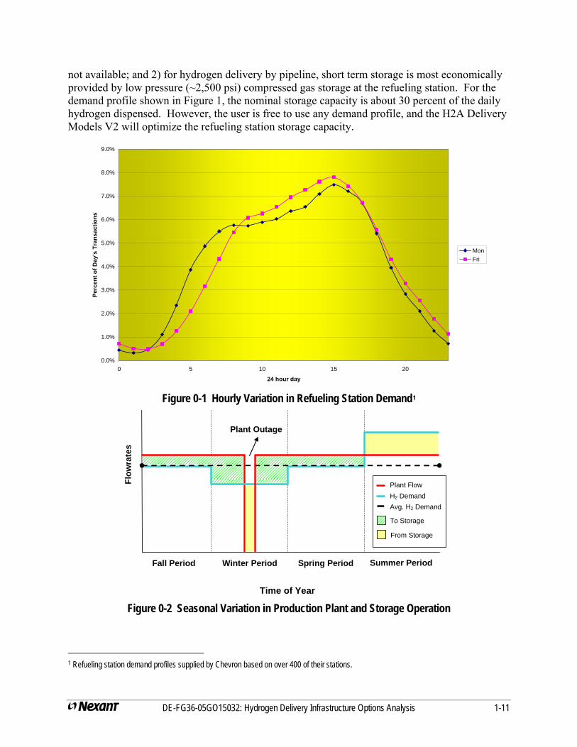
INFRASTRUCTURE STORAGE One of the principal activities in the project was to incorporate hydrogen storage in the delivery system to accommodate the unavoidable mismatches between production and demand. There are two storage requirements: a short term capacity for the hourly variation in refueling station demand; and a long term capacity for the seasonal variation in refueling station demand and production plant outages.
A representative hourly variation in refueling station demand is illustrated in Figure 0-1, and an illustration of the seasonal variation in demand, together with an annual production plant outage for scheduled maintenance, is shown in Figure 0-2. The seasonal demand variation is a product of annual driving profiles; i.e., miles driven in the summer are normally higher than miles driven in the winter.
A series of optimization studies concluded the following for gaseous hydrogen pipeline delivery pathways: 1) long term storage is most economically provided by compressed gas storage in geologic formations, if geologic storage is available, and in liquid storage, if geologic storage is
DE-FG36-05GO15032: Hydrogen Delivery Infrastructure Options Analysis 1-10
DE-FG36-05GO15032: Hydrogen Delivery Infrastructure Options Analysis 1-11
not available; and 2) for hydrogen delivery by pipeline, short term storage is most economically provided by low pressure (~2,500 psi) compressed gas storage at the refueling station. For the demand profile shown in Figure 1, the nominal storage capacity is about 30 percent of the daily hydrogen dispensed. However, the user is free to use any demand profile, and the H2A Delivery Models V2 will optimize the refueling station storage capacity.
0.0%
1.0%
2.0%
3.0%
4.0%
5.0%
6.0%
7.0%
8.0%
9.0%
0 5 10 15 20
24 hour day
Perc
ent o
f Day
's T
rans
actio
ns
MonFri
Figure 0-1 Hourly Variation in Refueling Station Demand1
Time of Year
Plant Outage
Flow
rate
s
Plant Flow H2 Demand Avg. H2 Demand
To Storage
From Storage
Summer Period Spring Period Winter Period Fall Period
Figure 0-2 Seasonal Variation in Production Plant and Storage Operation
1 Refueling station demand profiles supplied by Chevron based on over 400 of their stations.
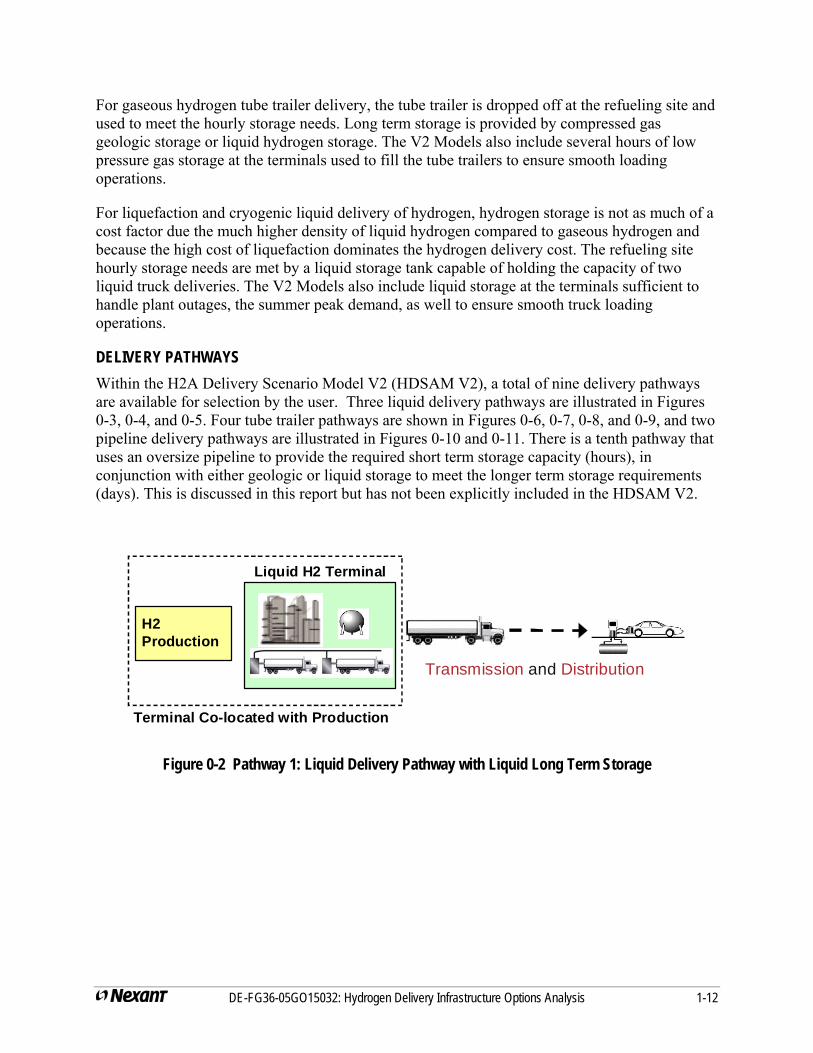
For gaseous hydrogen tube trailer delivery, the tube trailer is dropped off at the refueling site and used to meet the hourly storage needs. Long term storage is provided by compressed gas geologic storage or liquid hydrogen storage. The V2 Models also include several hours of low pressure gas storage at the terminals used to fill the tube trailers to ensure smooth loading operations.
For liquefaction and cryogenic liquid delivery of hydrogen, hydrogen storage is not as much of a cost factor due the much higher density of liquid hydrogen compared to gaseous hydrogen and because the high cost of liquefaction dominates the hydrogen delivery cost. The refueling site hourly storage needs are met by a liquid storage tank capable of holding the capacity of two liquid truck deliveries. The V2 Models also include liquid storage at the terminals sufficient to handle plant outages, the summer peak demand, as well to ensure smooth truck loading operations.
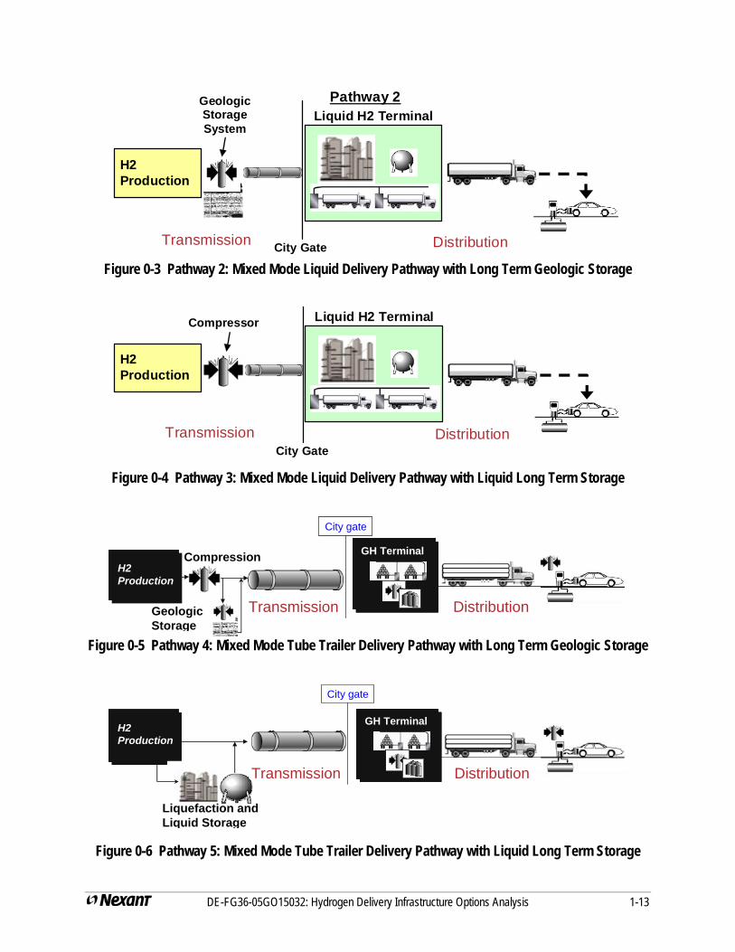
DELIVERY PATHWAYS Within the H2A Delivery Scenario Model V2 (HDSAM V2), a total of nine delivery pathways are available for selection by the user. Three liquid delivery pathways are illustrated in Figures 0-3, 0-4, and 0-5. Four tube trailer pathways are shown in Figures 0-6, 0-7, 0-8, and 0-9, and two pipeline delivery pathways are illustrated in Figures 0-10 and 0-11. There is a tenth pathway that uses an oversize pipeline to provide the required short term storage capacity (hours), in conjunction with either geologic or liquid storage to meet the longer term storage requirements (days). This is discussed in this report but has not been explicitly included in the HDSAM V2.
Transmission and Distribution
H2 Production
Liquid H2 Terminal
Terminal Co-located with Production
Figure 0-2 Pathway 1: Liquid Delivery Pathway with Liquid Long Term Storage
DE-FG36-05GO15032: Hydrogen Delivery Infrastructure Options Analysis 1-12
Pathway 2
H2 Production
Liquid H2 Terminal
City GateTransmission Distribution
Geologic Storage System
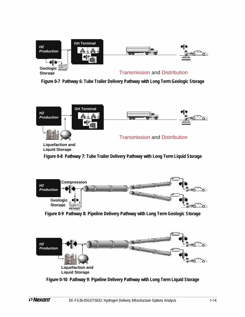
Figure 0-3 Pathway 2: Mixed Mode Liquid Delivery Pathway with Long Term Geologic Storage
H2 Production
Liquid H2 Terminal
City GateTransmission Distribution
Compressor
Figure 0-4 Pathway 3: Mixed Mode Liquid Delivery Pathway with Liquid Long Term Storage
GH TerminalGH TerminalH2 Production
City gate
Transmission Distribution
Compression
Geologic Storage
Figure 0-5 Pathway 4: Mixed Mode Tube Trailer Delivery Pathway with Long Term Geologic Storage
GH TerminalGH TerminalH2 ProductionH2 Production
City gate
Transmission Distribution
Liquefaction and Liquid Storage
Figure 0-6 Pathway 5: Mixed Mode Tube Trailer Delivery Pathway with Liquid Long Term Storage
DE-FG36-05GO15032: Hydrogen Delivery Infrastructure Options Analysis 1-13
GH TerminalGH TerminalH2 ProductionH2 Production
Transmission and Distribution
Geologic Storage
Figure 0-7 Pathway 6: Tube Trailer Delivery Pathway with Long Term Geologic Storage
H2 ProductionH2 Production
Transmission and Distribution
GH TerminalGH Terminal
Liquefaction and Liquid Storage Figure 0-8 Pathway 7: Tube Trailer Delivery Pathway with Long Term Liquid Storage
H2 ProductionH2 ProductionH2 Production
Compression
Geologic Storage
Figure 0-9 Pathway 8: Pipeline Delivery Pathway with Long Term Geologic Storage
H2 ProductionH2 ProductionH2 Production
Liquefaction and Liquid Storage
Figure 0-10 Pathway 9: Pipeline Delivery Pathway with Long Term Liquid Storage
DE-FG36-05GO15032: Hydrogen Delivery Infrastructure Options Analysis 1-14
H2A DELIVERY MODELS There are two H2A Delivery Models; the Components Model and the Hydrogen Delivery Scenario Model (HDSAM). The models and users guides are available at www.hydrogen.energy.gov/h2a_delivery.html.
The Components Model allows the user to examine the costs, energy efficiency and greenhouse gas (GHG) emissions of individual components (e.g. compressors, pipelines, liquefiers, terminals, etc.).
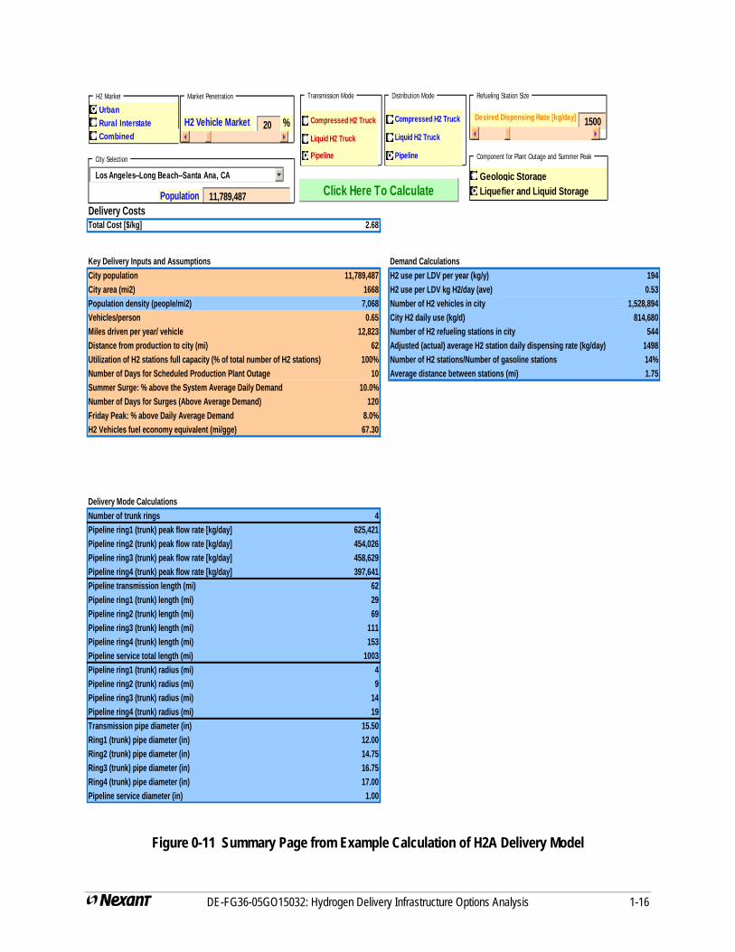
HDSAM V2 allows the user to select specific geographically based scenarios (e.g. a particular city, rural/interstate fueling, or combined city and rural interstate) and examine delivery costs as a function of hydrogen fuel cell vehicle market penetration. To run the HDSAM V2 model for a city, the user selects the following: city; market penetration; delivery pathway; and type of long term storage (geologic or liquid). HDSAM then calculates the following: infrastructure system capacities; short term storage capacities (for pipeline delivery pathways); long term storage capacities; delivery system capital cost; delivery system operating costs; levelized cost of hydrogen dispensed, energy efficiencies and GHG emissions. The basic inputs and summary results of a representative calculation are shown in Figure 0-12. In this example the calculations are performed for Los Angeles, California, with a market penetration of 20 percent. Hydrogen is delivered by pipeline, the average refueling station capacity is 1,500 kg/day, and long term storage is in the form of liquid hydrogen. For this set of parameters, the levelized cost to deliver hydrogen is $2.68 per kg.
In addition to using the H2A Delivery Models with their default values for current hydrogen delivery technologies, the models can be used to:
- Understand the key delivery cost drivers and the best delivery pathway for various markets and market penetrations.
- Quantify the overall delivery cost reduction possible based on replacing specific default values with lower costs or improved performance of one or more of the component technologies.
This ability can help guide the most effective R&D approach to reduce hydrogen delivery costs.
DE-FG36-05GO15032: Hydrogen Delivery Infrastructure Options Analysis 1-15
DE-FG36-05GO15032: Hydrogen Delivery Infrastructure Options Analysis 1-16
Delivery CostsTotal Cost [$/kg] 2.68
Key Delivery Inputs and Assumptions Demand CalculationsCity population 11,789,487 H2 use per LDV per year (kg/y) 194City area (mi2) 1668 H2 use per LDV kg H2/day (ave) 0.53Population density (people/mi2) 7,068 Number of H2 vehicles in city 1,528,894Vehicles/person 0.65 City H2 daily use (kg/d) 814,680Miles driven per year/ vehicle 12,823 Number of H2 refueling stations in city 544Distance from production to city (mi) 62 Adjusted (actual) average H2 station daily dispensing rate (kg/day) 1498Utilization of H2 stations full capacity (% of total number of H2 stations) 100% Number of H2 stations/Number of gasoline stations 1Number of Days for Scheduled Production Plant Outage 10 Average distance between stations (mi) 1.75Summer Surge: % above the System Average Daily Demand 10.0%Number of Days for Surges (Above Average Demand) 120Friday Peak: % above Daily Average Demand 8.0%H2 Vehicles fuel economy equivalent (mi/gge) 67.30
Delivery Mode CalculationsNumber of trunk rings 4Pipeline ring1 (trunk) peak flow rate [kg/day] 625,421Pipeline ring2 (trunk) peak flow rate [kg/day] 454,026Pipeline ring3 (trunk) peak flow rate [kg/day] 458,629Pipeline ring4 (trunk) peak flow rate [kg/day] 397,641Pipeline transmission length (mi) 62Pipeline ring1 (trunk) length (mi) 29Pipeline ring2 (trunk) length (mi) 69Pipeline ring3 (trunk) length (mi) 111Pipeline ring4 (trunk) length (mi) 153Pipeline service total length (mi) 1003Pipeline ring1 (trunk) radius (mi) 4Pipeline ring2 (trunk) radius (mi) 9Pipeline ring3 (trunk) radius (mi) 14Pipeline ring4 (trunk) radius (mi) 19Transmission pipe diameter (in) 15.50Ring1 (trunk) pipe diameter (in) 12.00Ring2 (trunk) pipe diameter (in) 14.75Ring3 (trunk) pipe diameter (in) 16.75Ring4 (trunk) pipe diameter (in) 17.00Pipeline service diameter (in) 1.00
4%
Distribution Mode
UrbanRural Interstate Compressed H2 Truck
Liquid H2 Truck
Pipeline
Los Angeles--Long Beach--Santa Ana, CA
20
11,789,487
%H2 Vehicle Market
Population
Market Penetration
City Selection
H2 Market
Click Here To Calculate
Transmission Mode
Compressed H2 Truck
Liquid H2 Truck
Pipeline
1500 Desired Dispensing Rate [kg/day]
Refueling Station Size
Geologic StorageLiquefier and Liquid Storage
Component for Plant Outage and Summer Peak
Combined
Figure 0-11 Summary Page from Example Calculation of H2A Delivery Model
SUMMARY OF RESULTS AND RECOMMENDATIONS The results of numerous HDSAM V2 model runs, over a wide range of market conditions, show the following general conclusions for currently available hydrogen delivery technologies:
At low market demands (<10% market penetration)with a central plant 62 or greater miles from the city, the delivery cost of hydrogen to refueling stations is high for all delivery modes ($5-$10/kg of hydrogen or even higher), suggesting that distributed production of hydrogen at refueling stations may serve the early markets for hydrogen vehicles. Alternatively a small semi-central plant located at the city gate may provide sufficiently low delivery cost by tube trailers.
If the city size is small (<400,000 people), if the market penetration is low (<10%), if the refueling station capacity is small (<400 kg/day), and if the distance to the production plant is modest (<62 miles), then hydrogen delivery by tube trailer is the lowest cost option. For early market conditions, delivery costs of $5 to $12/kg are anticipated.
If one or two market conditions move from the ‘small’ to the ‘large’ category, hydrogen delivery by liquid truck may be the lowest cost approach. However the energy consumed is 80% the energy in the hydrogen delivered due to the energy intensity of hydrogen liquefaction.
For a maturing hydrogen fuel cell vehicle market (>20% market penetration), hydrogen delivery by pipeline is almost universally preferred, with expected delivery costs in the range of $2 to $4/kg of hydrogen depending on the size of the city and market penetration level.
If the hydrogen production plants are located less than 62 miles from the “city gate” and if tube trailers are developed that could deliver about 1,000 kg of hydrogen, the cost of tube trailer delivery drops significantly and approaches the cost of pipeline delivery. This approach could avoid the required cost, time, disruption, and potential safety concerns of building hydrogen pipeline distribution systems in urban areas.
The energy use in the delivery of hydrogen can be significant. For pipeline delivery, tube trailer delivery and liquid hydrogen delivery the Well to Vehicle Tank energy use is about 30%, 35% and 80% of the energy in the hydrogen delivered respectively.
Greenhouse gas emissions are the lowest with pipeline delivery, moderately higher with tube trailer delivery, but essentially double with liquid delivery.
The cost of hydrogen delivery is a function of the market demand in terms of kg of hydrogen per square mile (determined by the population density, vehicle ownership rate, and % transportation vehicle market penetration) and the distance between the central manufacturing plant and the market. Thus delivery costs to the vast majority of the U.S.(>75% of the land area) can be reasonably modeled in HDSAM V2 by drawing large enough circles (markets) around each major city and defining the population density as a function of distance from the center of the circle.
There would be sufficient hydrogen demand to justify a central hydrogen production plant (50,000 to 350,000 kg/day of hydrogen production) located near any significant
DE-FG36-05GO15032: Hydrogen Delivery Infrastructure Options Analysis 1-17
urban area (>300,000 people) even at modest transportation vehicle market penetration (>25%). Large urban areas will require multiple large hydrogen production plants to supply them. As a result of this and the relatively high cost of hydrogen transport, it would be expected to have the production plant(s) located as close to the city as permitted. This is likely to be less than 62 miles from the “city gate” and quite possibly at the city’s edge.
Tube trailers, liquid truck delivery, and pipelines are each the optimum delivery method at different points in the maturation of the hydrogen infrastructure. As such, efforts to reduce the energy requirements and the capital cost of each method can reduce the overall costs of hydrogen delivery in the transition to and widespread use of hydrogen fuel cell vehicles. Possible research efforts include the following:
Lower cost composite based high pressure storage vessels for hydrogen storage and cascade charging systems at the refueling station. These storage vessels are a major cost for all delivery pathways.
Composite based high pressure (7,000 psi) tube trailers or other approaches to a tube trailer with a capacity of 1000 kg of hydrogen.
FRP transmission and or distribution pipelines to reduce pipeline capital and thus pipeline delivery costs. The distribution lines are the larger portion of the pipeline costs.
Magnetic, or other novel, methods for hydrogen liquefaction.
Finally possible enhancements to HDSAM V2 include:
Adding an option for 10,000 psi vehicle fills
Including, as required, the equipment to pre-cool the hydrogen gas prior to dispensing for 10,000 psi fills and vehicle hydride and sorbent storage approaches.
Adding novel hydrogen carriers to the delivery pathways. Potential carriers include metal hydrides/alanates, chemical hydrides, liquid phase hydrogen carriers, and high surface area sorbents. Preliminary studies indicate the latter two approaches hold some promise for hydrogen delivery.
Adding novel hydrogen carriers to the delivery pathways. Potential carriers include metal hydrides/alanates, chemical hydrides, liquid phase hydrogen carriers, and high surface area sorbents. Preliminary studies indicate the latter two approaches hold some promise for hydrogen delivery
Examining the use of cold (-50oC to -150oC) hydrogen compressed gas for delivery and vehicle storage.
DE-FG36-05GO15032: Hydrogen Delivery Infrastructure Options Analysis 1-18
Section 1 Introduction
In this project, the Nexant team has conducted an in-depth comparative analysis of various promising infrastructure options for hydrogen delivery and distribution to refueling stations from central, semi-central and distributed production facilities. The major objectives are to provide improved hydrogen delivery modeling capability and meaningful recommendations to DOE on the research strategy that will lead to cost effective and energy efficient hydrogen delivery infrastructure to meet the DOE delivery goals, which in turn will help enable the use of hydrogen as a major energy carrier for fuel cell vehicles and stationary power generation.
The project focuses on hydrogen supply for light-duty fuel cell vehicles but the results can be utilized for other hydrogen markets.
The project evaluates and analyzes the following six hydrogen delivery options:
Option 1: Dedicated pipelines for gaseous hydrogen delivery
Option 2: Use of existing natural gas or oil pipelines for gaseous hydrogen delivery
Option 3: Use of existing natural gas pipelines by blending in gaseous hydrogen with the separation of hydrogen from natural gas at the point of use
Option 4: Truck delivery of gaseous hydrogen
Option 5: Truck delivery of liquid hydrogen
Option 6: Use of novel solid or liquid H2 carriers in slurry/solvent form transported by pipeline/rail/trucks
The Nexant team conducted the project in six technical tasks:
Task 1: Collect and Compile Data and Knowledge Base
Task 2: Evaluate Current and Future Efficiencies and Costs of Hydrogen Delivery Options
Task 3: Evaluate Existing Infrastructure Capability for Hydrogen Delivery
Task 4: Assess GHG and Pollutant Emissions in Hydrogen Delivery
Task 5: Compare and Rank Delivery Options
Task 6: Recommend Hydrogen Delivery Strategies
The project team assembled to conduct this work consists of seven members. Air Liquide, GTI, and Nexant have the real world experience of building infrastructure projects and owning and operating hydrogen pipelines and other types of hydrogen delivery facilities. This real word experience can lead to meaningful and credible design and cost estimate for the various hydrogen delivery options and address the practical issues in the design. TIAX, Argonne National Lab (ANL), Pacific Northwest National Lab (PNNL), and the National Renewable Energy Lab (NREL) have the technology forward looking which can contribute to a successful identification and assessment of some promising delivery options currently still in the development, as well as the strong expertise and capability in delivery modeling. Chevron Technology Venture is the
DE-FG36-05GO15032: Hydrogen Delivery Infrastructure Options Analysis 1-19

DE-FG36-05GO15032: Hydrogen Delivery Infrastructure Options Analysis 1-20
ultimate user of the hydrogen delivered and can provide their valuable perspectives on the path for building the hydrogen economy.
This interim report will focus on Options 1, 4, 5, and 6 which have been incorporated into the H2A Delivery Components Model and Hydrogen Delivery Scenario Model (H2A Delivery Models) as Version (V2) of these models. The other pathways and final recommendations will be presented in the Final Nexant project report.
Section 2 H2A Hydrogen Delivery Models
2.1 MODEL DESIGN PARAMETERS Most of the effort on this project, as well as in H2A delivery modeling in general, focuses on currently available hydrogen delivery technologies. Thus, all of the components modeled in the default/base case (e.g. compressors, steel tanks, liquefaction units, steel pipelines, etc.) can be purchased and utilized now. Although hydrogen fuel cell vehicles are not generally available, these too are modeled as current technologies. Model inputs are based largely on analyses of cost data bases and vendor quotes, supplemented by industry review. All information sources are referenced in this report and/or in the models themselves.
2.1.1 Current Technology Characterization versus Future Projections To a large extent, the characteristics of current hydrogen delivery technology determine how the infrastructure can be modeled and optimized, and how well new technologies can be modeled. For example, the relationship between capital cost and pressure determines the optimum design and cost of conventional steel storage tanks. This relationship is explained in Sections 2.2.3 and 2.2.4. Although composite gas storage vessels are now being developed for off-board hydrogen storage, these cannot be modeled in the current H2A Delivery Models without extreme care because the capital cost vs. pressure relationship for these vessels differs from that of steel vessels, resulting in potentially different optima for storage pressure and cost. This, in turn, is likely to alter the optimum hydrogen delivery infrastructure storage scheme from that described in this report and utilized in the H2A Delivery Models.
Similarly, most current gaseous hydrogen vehicle refueling is to a 5,000 psi end-state fill pressure. Although research and development of 10,000 psi vehicle refueling is underway, components modeled in the H2A Delivery Models V2 can accommodate only 5,000 psi vehicle fills. Additional data on equipment costs and characteristics are needed to model 10,000 psi fills accurately.
On the other hand, the H2A Delivery Models are designed to accommodate a range of alternative assumptions, thereby providing considerable flexibility to the users. Many default inputs can be changed to examine various cases of interest. Some of these changes define alternative scenarios that would still utilize existing hydrogen delivery technology. Simple examples of this include varying the size of refueling stations, hours of storage at a terminal, or the frequency of truck deliveries. All these choices/inputs can be entered on the appropriate Excel spreadsheets in the H2A Delivery Models.
The H2A Delivery Models also allow the user to modify default values that characterize individual delivery components (e.g., capital cost of compressors or liquefaction plants, compressor efficiency, truck fuel economy, etc.). Users might choose to change any of these inputs to better reflect their own experience or to examine the impact of a potential change on the results or perhaps to reflect advances in technology. Care needs to be taken when making such changes, however, as they could impact the basic relationships and optimizations incorporated in
DE-FG36-05GO15032: Hydrogen Delivery Infrastructure Options Analysis 2-1
DE-FG36-05GO15032: Hydrogen Delivery Infrastructure Options Analysis 2-2
the models. This report and the H2A Delivery Model Users Guides2 contain the information needed by a skilled delivery analyst to avoid pitfalls when making such changes. A Help Desk is also available for specific questions.3
2.1.2 Fuel Cell Vehicle Operating Characteristics Within the H2A Delivery Models, the operating characteristics of fuel cell vehicles reflect the objectives of the US Department of Energy’s Multiyear Research, Development and Demonstration Plan for hydrogen and fuel cell vehicles. Those objectives are to develop a 60 percent peak-efficient, durable, direct hydrogen fuel cell power system at a cost of $45/kW by 2010 and $30/kW by 2015.4 As compared with a conventional spark-ignition (SI) gasoline-fueled vehicle, this translates into an average fuel economy for hydrogen FCVs of approxim58 miles per gasoline-gallon-equivalent (mpgge).
ately
5 The characteristics of the hydrogen FCV are taken from DOE’s ongoing Multipath Study,6 for which the PSAT model was run to generate estimates of conventional SI and FCV fuel economy for model year (MY) 2007 mid-sized automobiles.7 Both conventional and hydrogen LDVs are modeled as “average” vehicles (i.e., mid-sized automobiles). For modeling purposes, the conventional vehicle is assumed to be a MY 2007 vehicle that achieves a “rated” fuel economy of 29 mpg.8 The comparable 2007 MY FCV achieves a “rated” fuel economy of 58 mpgge.
Both gasoline and hydrogen LDVs are assumed to have a driving range of approximately 300 miles and to refuel at comparable intervals. Approximately 6 kg of hydrogen is assumed to be stored on board the vehicle (of which 5.6 kg or 95% is recoverable) 9 and to be supplied via a hydrogen production and delivery infrastructure. Note that the level of fuel efficiency assumed for hydrogen fuel cell vehicles is not appreciably greater that that obtained in current laboratory and field trials. The challenge is to achieve this efficiency while improving durability to a level comparable to conventional internal-combustion engines and also reducing the amount of precious metal catalysts and other expensive materials in the fuel-cell stack or replacing them with less expensive options.
In terms of other operating parameters, fuel cell vehicles are assumed to be driven the same number of annual miles as conventional vehicles, under the same road and climactic conditions, and with comparable vehicle loads. However, as with other defaults, the user can change fuel-cell vehicle fuel economy and annual utilization to reflect a desired scenario by making appropriate adjustments to model inputs.
2 US Department of Energy, Office of Hydrogen Fuel Cells and Infrastructure Technologies, accessed Oct. 2007 at
http://www.hydrogen.energy.gov/h2a_delivery/html. 3 Ibid. 4 US Department of Energy, Office of Hydrogen Fuel Cells and Infrastructure Technologies, Multiyear Research, Development and
Demonstration Plan, April 2007 accessed Oct. 2007 at http://www1.eere.energy.gov/hydrogenandfuelcells/mypp. 5 A gasoline gallon-equivalent (gge) is the amount of hydrogen that has the same energy content (on a lower heating value basis) as a gallon
of gasoline. A gallon of gasoline contains approximately 116,000 Btu, roughly equivalent to the energy content of 1 kilogram of hydrogen. 6 S. Plotkin, Argonne National Laboratory, personal communication, Nov. 21, 2007. 7 A. Rousseau, Argonne National Laboratory, personal communication, Nov. 20, 2007. For further information on PSAT (Powertrain Systems
Analysis Toolkit) see http://www.anl.gov/Media_Center/News/2006/news061219.html. 8 “Rated” or test fuel economy is estimated over a driving cycle which simulates a combination of urban and suburban driving. Actual fuel
economy typically is considerably less for conventional IC vehicles. For FCVs there are no data to estimate actual fuel economy. In 2005 the entire fleet of gasoline-fueled LDVs achieved approximately 20.2 mpg.
9 Personal communication, R. Ahluwalia,Argonne National Laboratory, Oct. 2007.
DE-FG36-05GO15032: Hydrogen Delivery Infrastructure Options Analysis 2-3
2.1.3 Refueling Station Characteristics In the delivery infrastructure bringing hydrogen motor fuel from centralized production facilities to hydrogen-fueled vehicles, hydrogen refueling stations will serve much the same function as today’s gasoline stations. They will dispense hydrogen, gasoline and perhaps other fuels, and will sell various convenience items. Aside from restrictions governing setback and separation distances, their footprint will be comparable to that of conventional gasoline stations. And they will serve similar numbers of vehicles with similar demand profiles. Modeling hydrogen refueling thus requires an understanding of gasoline refueling both at the macro and micro level.
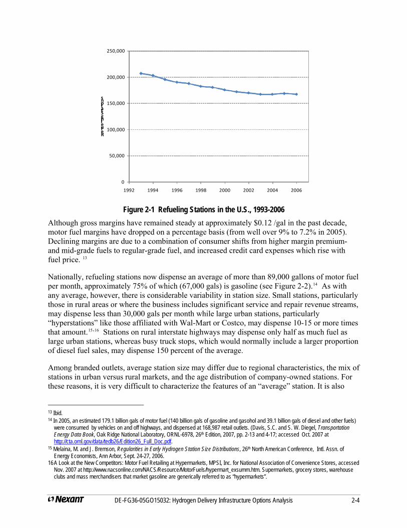
Gasoline retailing has evolved in the past several years. The number of retail outlets declined from over 210,000 in 1993 to 167,476 in 2005, a drop of nearly 20% (see Figure 2-1), while productivity (measured in terms of average sales per outlet) grew over 60%. No single factor has been identified for productivity gains, but as the DOE’s Energy Information Administration stated in a recent report, “there are many reasons for the increased intensity in the use of retail outlets … Introduction of higher-cost Phase I diesel and motor gasoline in the early 1990's (required by the 1990 Clean Air Act Amendments) tended to increase the costs to retailers. Additionally, underground storage tank requirements that generally became effective at the end of 1998 elevated the costs of those remaining in the industry. These factors tended to squeeze marginal operators, some of whom probably exited the industry. Increases in some retailing costs elicited efforts by retailers to reduce other costs, including using the fixed assets (e.g., the retail outlet and its location) more intensely by shoehorning more goods and services into the outlet and expanding operating hours.”10
While new environmental regulations raised costs, revenue streams from traditional automotive service and repair were eroded by the increased dependability and complexity of motor vehicles and the rise of “quick lubes”, tire warehouses and other specialty retailers. Refueling stations sought replacement revenue to augment essentially flat motor gasoline and lubricant revenues – first from the sale of convenience items and more recently from the sale of branded fast food and ATM transactions. Today, refueling stations that include convenience stores account for an estimated 75% of motor fuel sales.11 It should be noted, however, that while motor fuel represents more than two-thirds of the sales dollars at refueling stations that include convenience stores, it accounts for only a third of their profits.12
10 US DOE, Energy Information Administration, Restructuring: The Changing Face of Motor Gasoline Marketing, accessed Nov. 2007 at
http://www.eia.doe.gov/emeu/finance/sptopics/downstrm00/index.html. 11 Convenience Store Industry Sales Hit New Highs in 2005, National Association of Convenience Stores, accessed Nov. 2007 at
http://www.nacsonline.com/NACS/News/Press_Releases/2006/pr040506.htm. 12 Ibid.
DE-FG36-05GO15032: Hydrogen Delivery Infrastructure Options Analysis 2-4
0
50,000
100,000
150,000
200,000
250,000
1992 1994 1996 1998 2000 2002 2004 2006
Refueling Stations
Figure 2-1 Refueling Stations in the U.S., 1993-2006 Although gross margins have remained steady at approximately $0.12 /gal in the past decade, motor fuel margins have dropped on a percentage basis (from well over 9% to 7.2% in 2005). Declining margins are due to a combination of consumer shifts from higher margin premium- and mid-grade fuels to regular-grade fuel, and increased credit card expenses which rise with fuel price. 13
Nationally, refueling stations now dispense an average of more than 89,000 gallons of motor fuel per month, approximately 75% of which (67,000 gals) is gasoline (see Figure 2-2).14 As with any average, however, there is considerable variability in station size. Small stations, particularly those in rural areas or where the business includes significant service and repair revenue streams, may dispense less than 30,000 gals per month while large urban stations, particularly “hyperstations” like those affiliated with Wal-Mart or Costco, may dispense 10-15 or more times that amount.15,16 Stations on rural interstate highways may dispense only half as much fuel as large urban stations, whereas busy truck stops, which would normally include a larger proportion of diesel fuel sales, may dispense 150 percent of the average.
Among branded outlets, average station size may differ due to regional characteristics, the mix of stations in urban versus rural markets, and the age distribution of company-owned stations. For these reasons, it is very difficult to characterize the features of an “average” station. It is also
13 Ibid. 14 In 2005, an estimated 179.1 billion gals of motor fuel (140 billion gals of gasoline and gasohol and 39.1 billion gals of diesel and other fuels)
were consumed by vehicles on and off highways, and dispensed at 168,987 retail outlets. (Davis, S.C. and S. W. Diegel, Transportation Energy Data Book, Oak Ridge National Laboratory, ORNL-6978, 26th Edition, 2007, pp. 2-13 and 4-17; accessed Oct. 2007 at http://cta.ornl.gov/data/tedb26/Edition26_Full_Doc.pdf.
15 Melaina, M. and J. Bremson, Regularities in Early Hydrogen Station Size Distributions, 26th North American Conference, Intl. Assn. of Energy Economists, Ann Arbor, Sept. 24-27, 2006.
16 A Look at the New Competitors: Motor Fuel Retailing at Hypermarkets, MPSI, Inc. for National Association of Convenience Stores, accessed Nov. 2007 at http://www.nacsonline.com/NACS/Resource/MotorFuels/hypermart_exsumm.htm. Supermarkets, grocery stores, warehouse clubs and mass merchandisers that market gasoline are generically referred to as “hypermarkets”.
DE-FG36-05GO15032: Hydrogen Delivery Infrastructure Options Analysis 2-5
difficult to obtain what are often internal data on the operations of company-owned stations. Fortunately, the Nexant team included Chevron, whose staff provided the team with typical operating characteristics of Chevron refueling stations located primarily in Florida, California and Washington State.17 Based on these data, it is clear that Chevron’s average station is larger than the national average, typically dispensing 135,000 gals of gasoline per month from six multi-fuel pumping dispensers (12 hoses). Newer Chevron stations are even larger, designed to dispense up to 300,000 gals per month from six dispensers.
In addition to capacity increases, stations are also becoming more capital intensive. According to the Energy Information Administration, US majors’ retail outlets rose from an average of $500,000 net investment in place per outlet in 1990 to $771,000 in 1999.18 Although some of the increase undoubtedly came from the divestiture of marginal (generally smaller) outlets, capital investment in retailing outlets rose over the decade, suggesting real increases.
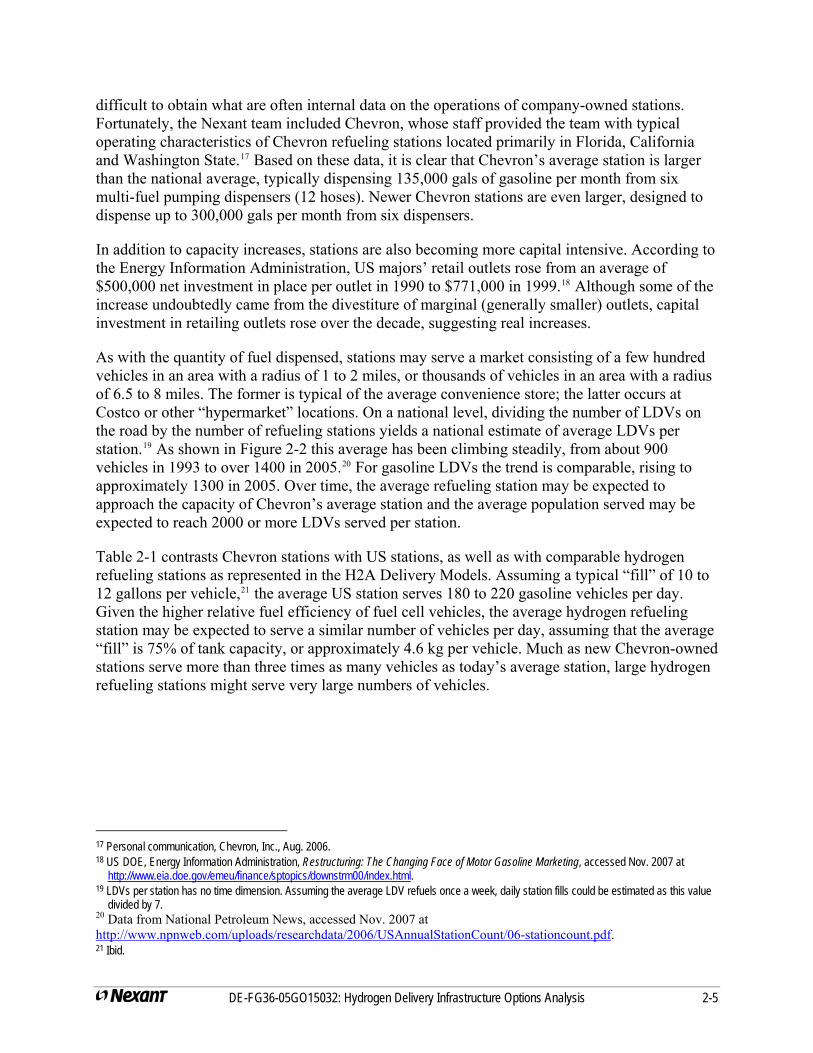
As with the quantity of fuel dispensed, stations may serve a market consisting of a few hundred vehicles in an area with a radius of 1 to 2 miles, or thousands of vehicles in an area with a radius of 6.5 to 8 miles. The former is typical of the average convenience store; the latter occurs at Costco or other “hypermarket” locations. On a national level, dividing the number of LDVs on the road by the number of refueling stations yields a national estimate of average LDVs per station.19 As shown in Figure 2-2 this average has been climbing steadily, from about 900 vehicles in 1993 to over 1400 in 2005.20 For gasoline LDVs the trend is comparable, rising to approximately 1300 in 2005. Over time, the average refueling station may be expected to approach the capacity of Chevron’s average station and the average population served may be expected to reach 2000 or more LDVs served per station.
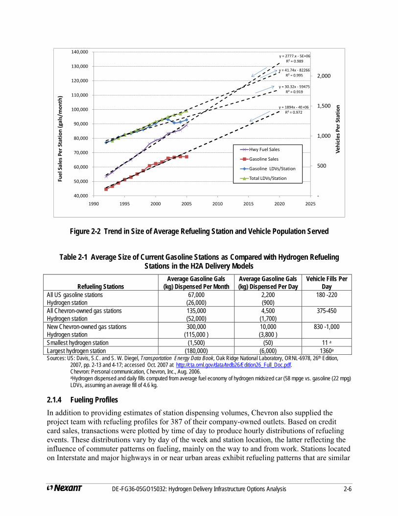
Table 2-1 contrasts Chevron stations with US stations, as well as with comparable hydrogen refueling stations as represented in the H2A Delivery Models. Assuming a typical “fill” of 10 to 12 gallons per vehicle,21 the average US station serves 180 to 220 gasoline vehicles per day. Given the higher relative fuel efficiency of fuel cell vehicles, the average hydrogen refueling station may be expected to serve a similar number of vehicles per day, assuming that the average “fill” is 75% of tank capacity, or approximately 4.6 kg per vehicle. Much as new Chevron-owned stations serve more than three times as many vehicles as today’s average station, large hydrogen refueling stations might serve very large numbers of vehicles.
17 Personal communication, Chevron, Inc., Aug. 2006. 18 US DOE, Energy Information Administration, Restructuring: The Changing Face of Motor Gasoline Marketing, accessed Nov. 2007 at
http://www.eia.doe.gov/emeu/finance/sptopics/downstrm00/index.html. 19 LDVs per station has no time dimension. Assuming the average LDV refuels once a week, daily station fills could be estimated as this value
divided by 7. 20 Data from National Petroleum News, accessed Nov. 2007 at http://www.npnweb.com/uploads/researchdata/2006/USAnnualStationCount/06-stationcount.pdf. 21 Ibid.
y = 2777.x ‐ 5E+06R² = 0.989
y = 1894x ‐ 4E+06R² = 0.972
y = 30.32x ‐ 59475R² = 0.919
y = 41.74x ‐ 82266R² = 0.995
‐
500
1,000
1,500
2,000
40,000
50,000
60,000
70,000
80,000
90,000
100,000
110,000
120,000
130,000
140,000
1990 1995 2000 2005 2010 2015 2020 2025
Vehicles Per Station
Fuel Sales Per Station
(gals/mon
th)
Hwy Fuel Sales
Gasoline Sales
Gasoline LDVs/Station
Total LDVs/Station
Figure 2-2 Trend in Size of Average Refueling Station and Vehicle Population Served
Table 2-1 Average Size of Current Gasoline Stations as Compared with Hydrogen Refueling Stations in the H2A Delivery Models
Refueling Stations Average Gasoline Gals
(kg) Dispensed Per Month Average Gasoline Gals (kg) Dispensed Per Day
Vehicle Fills Per Day
All US gasoline stations Hydrogen station
67,000 (26,000)
2,200 (900)
180 -220
All Chevron-owned gas stations Hydrogen station
135,000 (52,000)
4,500 (1,700)
375-450
New Chevron-owned gas stations Hydrogen station
300,000 (115,000 )
10,000 (3,800 )
830 -1,000
Smallest hydrogen station (1,500) (50) 11 a Largest hydrogen station (180,000) (6,000) 1360a Sources: US: Davis, S.C. and S. W. Diegel, Transportation Energy Data Book, Oak Ridge National Laboratory, ORNL-6978, 26th Edition,
2007, pp. 2-13 and 4-17; accessed Oct. 2007 at http://cta.ornl.gov/data/tedb26/Edition26_Full_Doc.pdf. Chevron: Personal communication, Chevron, Inc., Aug. 2006. aHydrogen dispensed and daily fills computed from average fuel economy of hydrogen midsized car (58 mpge vs. gasoline (22 mpg)
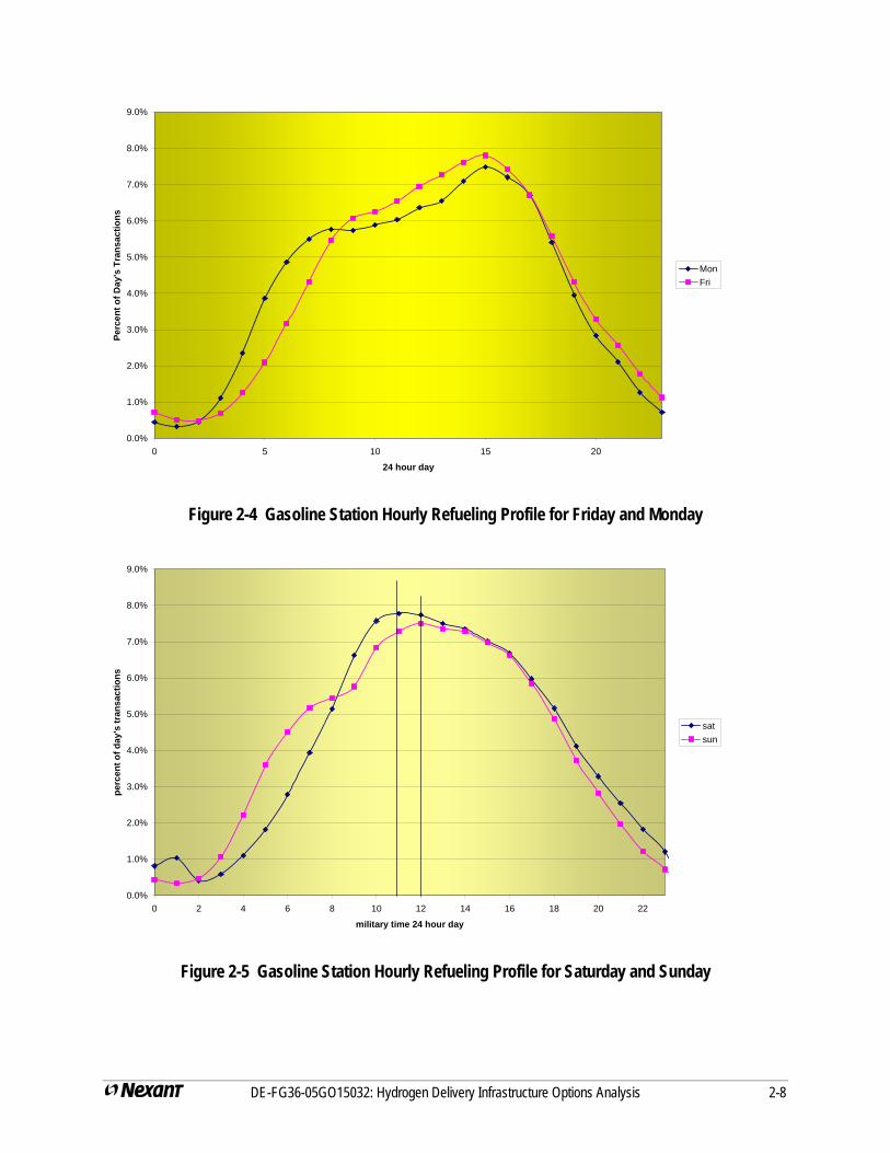
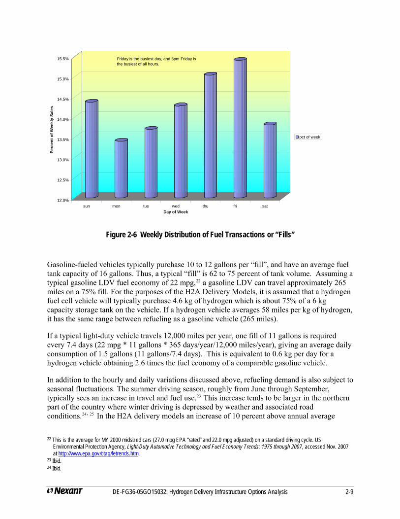
LDVs, assuming an average fill of 4.6 kg. 2.1.4 Fueling Profiles In addition to providing estimates of station dispensing volumes, Chevron also supplied the project team with refueling profiles for 387 of their company-owned outlets. Based on credit card sales, transactions were plotted by time of day to produce hourly distributions of refueling events. These distributions vary by day of the week and station location, the latter reflecting the influence of commuter patterns on fueling, mainly on the way to and from work. Stations located on Interstate and major highways in or near urban areas exhibit refueling patterns that are similar
DE-FG36-05GO15032: Hydrogen Delivery Infrastructure Options Analysis 2-6
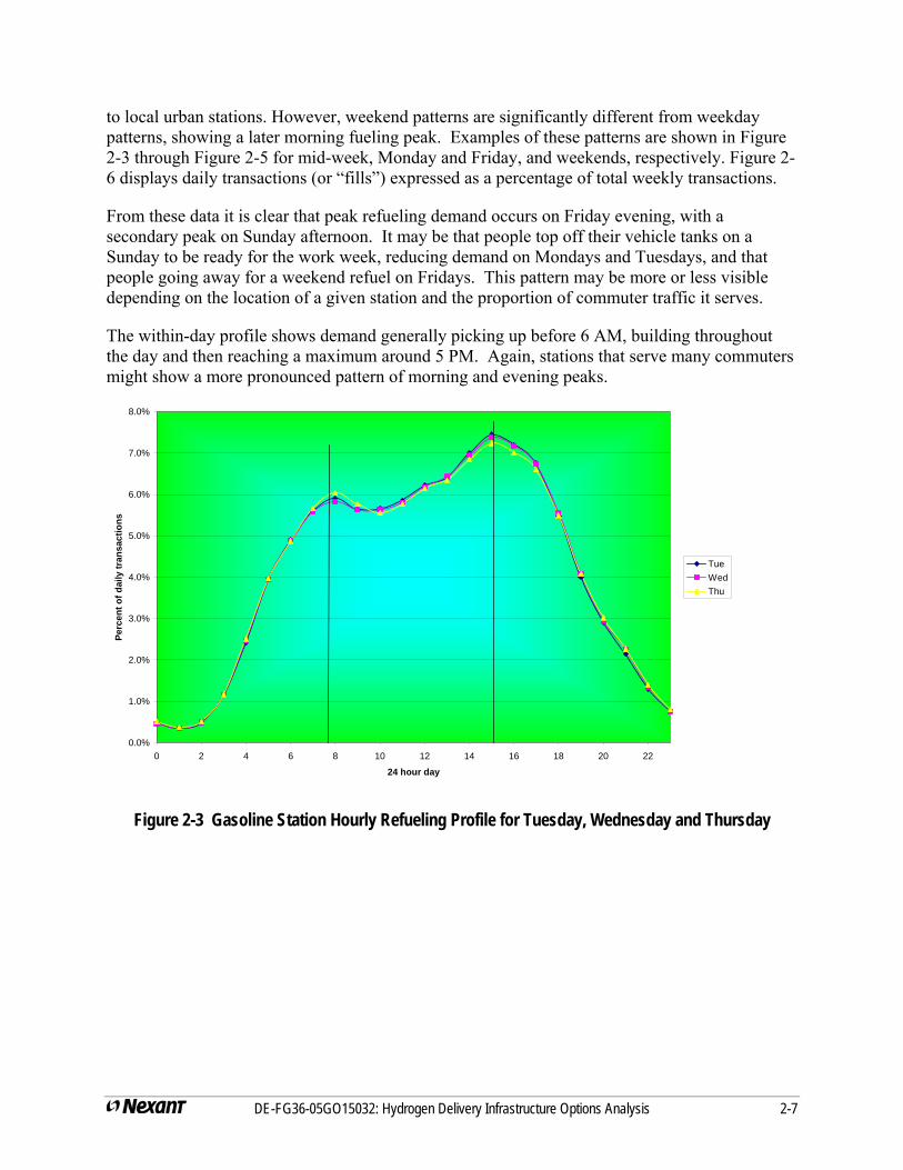
to local urban stations. However, weekend patterns are significantly different from weekday patterns, showing a later morning fueling peak. Examples of these patterns are shown in Figure 2-3 through Figure 2-5 for mid-week, Monday and Friday, and weekends, respectively. Figure 2-6 displays daily transactions (or “fills”) expressed as a percentage of total weekly transactions.
From these data it is clear that peak refueling demand occurs on Friday evening, with a secondary peak on Sunday afternoon. It may be that people top off their vehicle tanks on a Sunday to be ready for the work week, reducing demand on Mondays and Tuesdays, and that people going away for a weekend refuel on Fridays. This pattern may be more or less visible depending on the location of a given station and the proportion of commuter traffic it serves.
The within-day profile shows demand generally picking up before 6 AM, building throughout the day and then reaching a maximum around 5 PM. Again, stations that serve many commuters might show a more pronounced pattern of morning and evening peaks.
0.0%
1.0%
2.0%
3.0%
4.0%
5.0%
6.0%
7.0%
8.0%
0 2 4 6 8 10 12 14 16 18 20 22
24 hour day
Perc
ent o
f dai
ly tr
ansa
ctio
ns
TueWedThu
Figure 2-3 Gasoline Station Hourly Refueling Profile for Tuesday, Wednesday and Thursday
DE-FG36-05GO15032: Hydrogen Delivery Infrastructure Options Analysis 2-7
0.0%
1.0%
2.0%
3.0%
4.0%
5.0%
6.0%
7.0%
8.0%
9.0%
0 5 10 15 20
24 hour day
Perc
ent o
f Day
's T
rans
actio
ns
MonFri
Figure 2-4 Gasoline Station Hourly Refueling Profile for Friday and Monday
0.0%
1.0%
2.0%
3.0%
4.0%
5.0%
6.0%
7.0%
8.0%
9.0%
0 2 4 6 8 10 12 14 16 18 20 22
military time 24 hour day
perc
ent o
f day
's tr
ansa
ctio
ns
satsun
Figure 2-5 Gasoline Station Hourly Refueling Profile for Saturday and Sunday
DE-FG36-05GO15032: Hydrogen Delivery Infrastructure Options Analysis 2-8
DE-FG36-05GO15032: Hydrogen Delivery Infrastructure Options Analysis 2-9
12.0%
12.5%
13.0%
13.5%
14.0%
14.5%
15.0%
15.5%
Perc
ent o
f Wee
kly
Sale
s
sun mon tue wed thu fri satDay of Week
pct of week
Friday is the busiest day, and 5pm Friday is the busiest of all hours.
Figure 2-6 Weekly Distribution of Fuel Transactions or “Fills”
Gasoline-fueled vehicles typically purchase 10 to 12 gallons per “fill”, and have an average fuel tank capacity of 16 gallons. Thus, a typical “fill” is 62 to 75 percent of tank volume. Assuming a typical gasoline LDV fuel economy of 22 mpg,22 a gasoline LDV can travel approximately 265 miles on a 75% fill. For the purposes of the H2A Delivery Models, it is assumed that a hydrogen fuel cell vehicle will typically purchase 4.6 kg of hydrogen which is about 75% of a 6 kg capacity storage tank on the vehicle. If a hydrogen vehicle averages 58 miles per kg of hydrogen, it has the same range between refueling as a gasoline vehicle (265 miles).
If a typical light-duty vehicle travels 12,000 miles per year, one fill of 11 gallons is required every 7.4 days (22 mpg * 11 gallons * 365 days/year/12,000 miles/year), giving an average daily consumption of 1.5 gallons (11 gallons/7.4 days). This is equivalent to 0.6 kg per day for a hydrogen vehicle obtaining 2.6 times the fuel economy of a comparable gasoline vehicle.
In addition to the hourly and daily variations discussed above, refueling demand is also subject to seasonal fluctuations. The summer driving season, roughly from June through September, typically sees an increase in travel and fuel use.23 This increase tends to be larger in the northern part of the country where winter driving is depressed by weather and associated road conditions.24, 25 In the H2A delivery models an increase of 10 percent above annual average
22 This is the average for MY 2000 midsized cars (27.0 mpg EPA “rated” and 22.0 mpg adjusted) on a standard driving cycle. US
Environmental Protection Agency, Light-Duty Automotive Technology and Fuel Economy Trends: 1975 through 2007, accessed Nov. 2007 at http://www.epa.gov/otaq/fetrends.htm.
23 Ibid. 24 Ibid.
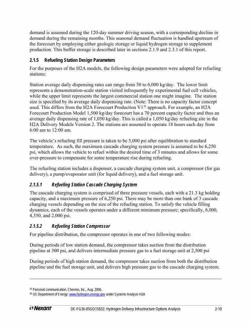
DE-FG36-05GO15032: Hydrogen Delivery Infrastructure Options Analysis 2-10
demand is assumed during the 120-day summer driving season, with a corresponding decline in demand during the remaining months. This seasonal demand fluctuation is handled upstream of the forecourt by employing either geologic storage or liquid hydrogen storage to supplement production. This buffer storage is described later in sections 2.1.9 and 2.3.1 of this report.
2.1.5 Refueling Station Design Parameters For the purposes of the H2A models, the following design parameters were adopted for refueling stations:
Station average daily dispensing rates can range from 50 to 6,000 kg/day. The lower limit represents a demonstration-scale station visited infrequently by experimental fuel cell vehicles, while the upper limit represents the largest commercial station one might imagine. The station size is specified by its average daily dispensing rate. (Note: There is no capacity factor concept used. This differs from the H2A Forecourt Production V126 approach. For example, an H2A Forecourt Production Model 1,500 kg/day forecourt has a 70 percent capacity factor and thus an average daily dispensing rate of 1,050 kg/day. This is called a 1,050 kg/day refueling site in the H2A Delivery Models Version 2. The stations are assumed to operate 18 hours each day from 6:00 am to 12:00 am.
The vehicle’s refueling fill pressure is taken to be 5,000 psi after equilibration to standard temperature. As such, the maximum cascade charging system pressure is assumed to be 6,250 psi, which allows the vehicle to refuel within the desired time of 3 minutes and allows for some over-pressure to compensate for some temperature rise during refueling.
The refueling station includes a dispenser, a cascade charging system unit, a compressor (for gas delivery), a pump/evaporator unit (for liquid delivery), and a fuel storage unit.
2.1.5.1 Refueling Station Cascade Charging System The cascade charging system is comprised of three pressure vessels, each with a 21.3 kg holding capacity, and a maximum pressure of 6,250 psi. There may be more than one bank of 3 cascade charging vessels depending on the size of the refueling station. To satisfy the vehicle filling dynamics, each of the vessels operates under a different minimum pressure; specifically, 6,000, 4,350, and 2,000 psi.
2.1.5.2 Refueling Station Compressor For pipeline distribution, the compressor operates in one of two following modes:
During periods of low station demand, the compressor takes suction from the distribution pipeline at 300 psi, and delivers intermediate pressure gas to a fuel storage unit at 2,500 psi
During periods of high station demand, the compressor takes suction from both the distribution pipeline and the fuel storage unit, and delivers high pressure gas to the cascade charging system.
25 Personal communication, Chevron, Inc., Aug. 2006. 26 US Department of Energy: www.hydrogen.energy.gov under Systems Analysis-H2A
For compressed gas tube trailer truck distribution, the compressor takes suction from the tube trailer, and delivers high pressure gas to the cascade charging system.
2.1.5.3 Refueling Station Liquid, Storage Pump and Evaporator While the gaseous refueling stations employ a compressor to charge the cascade system, the liquid refueling stations employ a pump and an evaporator to achieve the same goal. The pump takes suction from the liquid storage tank pressure, and raises the pressure to the cascade charging system pressure. The high pressure liquid is then gasified in the evaporator, and heated to the cascade operating temperature. The cryogenic liquid storage tanks at the refueling station are sized to satisfy the station average daily demand, and to limit the number of liquid truck deliveries to a maximum of three stations per trip.
2.1.5.4 Refueling Station Hydrogen Storage Unit The hydrogen storage consists of one of the following: pressurized tube trailers in the case of compressed gas truck distribution; cryogenic liquid tanks in the case of liquid truck distribution; and low pressure gas storage tanks for pipeline distribution.
Low pressure storage tanks are needed for pipeline distribution systems to absorb the difference between the (constant) flow rate from a production plant and the large hourly variation in refueling demand. As discussed in Section 2.2.3, the optimum operating pressure and holding capacity were found to be 2,500 psi and 91 kg, respectively.
2.1.6 Transmission and Distribution Pipeline Pressures There are three stages of pipeline included in the H2A models for urban deliveries: transmission, distribution trunk; and distribution service lines. The arrangement is similar to that for natural gas transmission and distribution.
Hydrogen gas is moved from the production plant to the city gate through large, high pressure transmission lines. At the city gate, the pressure is reduced, and the gas is moved through trunk pipelines for the distribution system. In the distribution service pipelines, the pressure is once more reduced, and the gas is distributed to the refueling stations. In all cases, the hydrogen pressure is reduced through a combination of pressure drop through the pipeline, and a pressure reduction valve and/or system. A flow diagram of the system is shown in Figure 2-7.
DE-FG36-05GO15032: Hydrogen Delivery Infrastructure Options Analysis 2-11
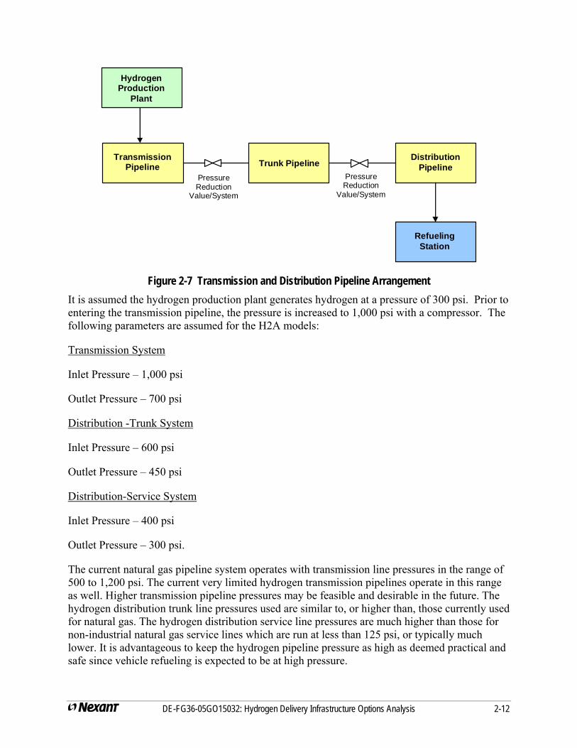
Transmission Pipeline Trunk Pipeline
Distribution Pipeline
Hydrogen Production
Plant
Refueling Station
Pressure Reduction
Value/System
Pressure Reduction
Value/System
Figure 2-7 Transmission and Distribution Pipeline Arrangement It is assumed the hydrogen production plant generates hydrogen at a pressure of 300 psi. Prior to entering the transmission pipeline, the pressure is increased to 1,000 psi with a compressor. The following parameters are assumed for the H2A models:
Transmission System
Inlet Pressure – 1,000 psi
Outlet Pressure – 700 psi
Distribution -Trunk System
Inlet Pressure – 600 psi
Outlet Pressure – 450 psi
Distribution-Service System
Inlet Pressure – 400 psi
Outlet Pressure – 300 psi.
The current natural gas pipeline system operates with transmission line pressures in the range of 500 to 1,200 psi. The current very limited hydrogen transmission pipelines operate in this range as well. Higher transmission pipeline pressures may be feasible and desirable in the future. The hydrogen distribution trunk line pressures used are similar to, or higher than, those currently used for natural gas. The hydrogen distribution service line pressures are much higher than those for non-industrial natural gas service lines which are run at less than 125 psi, or typically much lower. It is advantageous to keep the hydrogen pipeline pressure as high as deemed practical and safe since vehicle refueling is expected to be at high pressure.
DE-FG36-05GO15032: Hydrogen Delivery Infrastructure Options Analysis 2-12
2.1.7 Gaseous Tube Trailer Delivery Parameters A tube trailer incorporates nine tubes, each with a volume of 91.8 ft3. The holding capacity of the trailer is 344 kg with a tube pressure of 2,650 psi. The tube trailer can not be completely discharged. The H2A Delivery models assume a final discharge pressure of 220 psig and thus a delivered capacity of 280 kg. The models also allow the user to change the tube trailer inputs to model a 5,000 psi trailer that would have a holding capacity of 650 kg. Such technology is under development.
The loading time is assumed to be 6 hours and 10 hours for tube pressures of 2,650 psi and 5,000 psi, respectively. The pick-up and drop-off times at the terminal and the refueling stations, including connection and disconnection times, are assumed to be 1 hour and ½ hour, respectively.
The truck is assumed to be powered by a Diesel engine with a fuel economy of 5 mpg. The truck average speed is assumed to be 43 mph on the highway, and 25 mph in the city. The truck operates 18 hours per day, consistent with the refueling stations operational hours. The yearly truck availability is assumed to be 98 percent.
2.1.8 Liquid Truck Delivery Parameters The liquid truck tank volume is assumed to be approximately 17,000 gallon, with a nominal holding capacity of 4,600 kg. A heel of liquid hydrogen must be left in the truck so its delivered capacity is 4,110 kg.
The truck fill time is assumed to be 2 hours, to which is added 1 hour for connection, disconnection, and parking at the terminal. It is assumed the truck can make a maximum of three stops at refueling stations per trip. The unloading times are assumed to be 3.5, 2.5, and 2.0 hours for 1, 2, and 3 stops, respectively.
The operating parameters for the liquid delivery truck, such as average speed on the highway, are assumed to be the same as for the tube trailer truck.
2.1.9 Infrastructure Supply and Demand Variations and Storage Requirements With a fully commercial hydrogen infrastructure, a network of transmission lines or truck delivery will likely connect a group of production plants with various local cities. As such, a maintenance outage on a particular plant is not likely to cause a severe disruption of hydrogen delivery, as the other plants in the network might accommodate the deficit. However, in the early phases of the infrastructure development, only one production plant may supply a city, and some form of long term storage will be necessary to accommodate production plant outages such as for annual maintenance. In addition, as discussed in Section 2.1.3, there is a seasonal variation in gasoline demand. Specifically, the summer demand is approximately 10 percent higher than the annual average, and the winter demand is 10 percent lower. Thus, the long term storage system must store the excess production in the winter, and deliver the stored hydrogen to supplement the production supply in the summer.
For the purposes of the H2A models, an annual schedule of production and demand was developed, as illustrated in Figure 2-8.
DE-FG36-05GO15032: Hydrogen Delivery Infrastructure Options Analysis 2-13
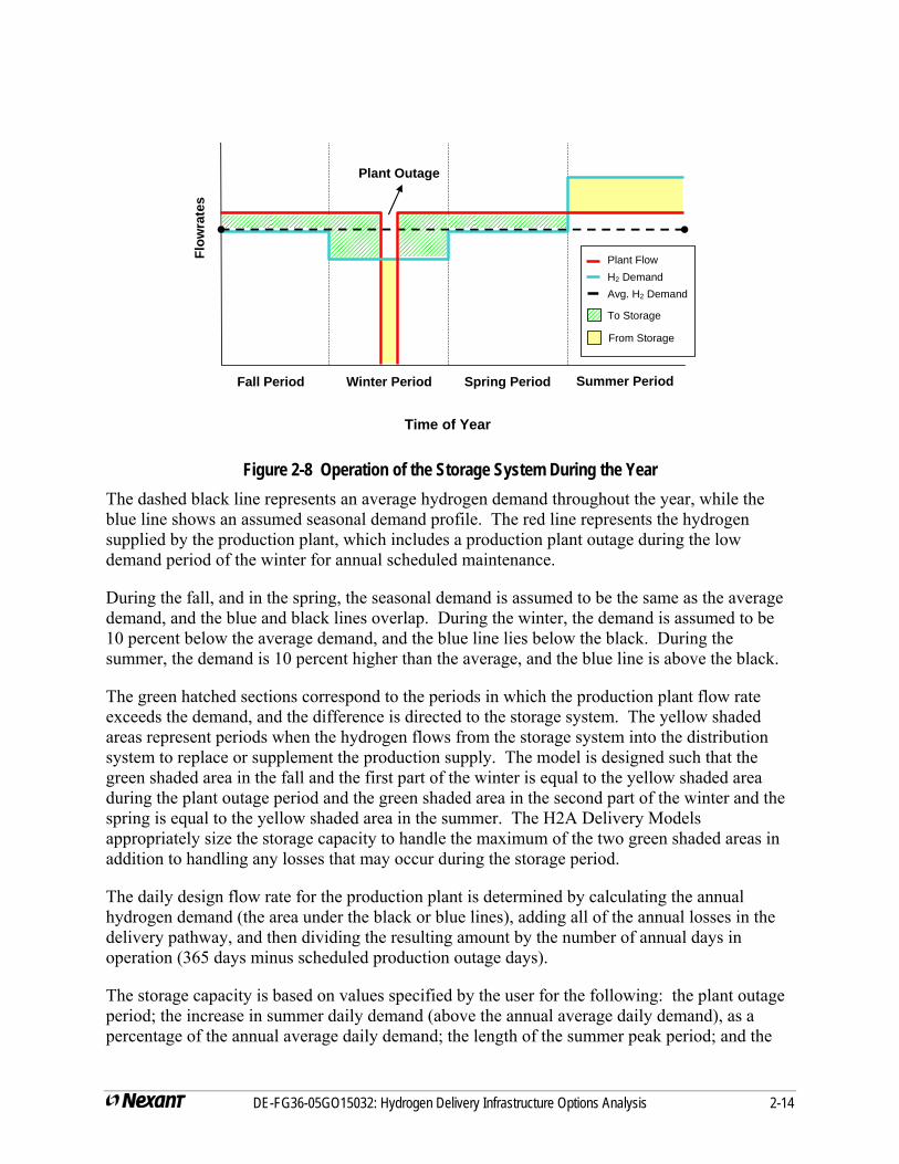
Time of Year
Plant Outage
Flow
rate
s
Plant Flow H2 Demand Avg. H2 Demand
To Storage
From Storage
Summer Period Spring Period Winter Period Fall Period
Figure 2-8 Operation of the Storage System During the Year The dashed black line represents an average hydrogen demand throughout the year, while the blue line shows an assumed seasonal demand profile. The red line represents the hydrogen supplied by the production plant, which includes a production plant outage during the low demand period of the winter for annual scheduled maintenance.
During the fall, and in the spring, the seasonal demand is assumed to be the same as the average demand, and the blue and black lines overlap. During the winter, the demand is assumed to be 10 percent below the average demand, and the blue line lies below the black. During the summer, the demand is 10 percent higher than the average, and the blue line is above the black.
The green hatched sections correspond to the periods in which the production plant flow rate exceeds the demand, and the difference is directed to the storage system. The yellow shaded areas represent periods when the hydrogen flows from the storage system into the distribution system to replace or supplement the production supply. The model is designed such that the green shaded area in the fall and the first part of the winter is equal to the yellow shaded area during the plant outage period and the green shaded area in the second part of the winter and the spring is equal to the yellow shaded area in the summer. The H2A Delivery Models appropriately size the storage capacity to handle the maximum of the two green shaded areas in addition to handling any losses that may occur during the storage period.
The daily design flow rate for the production plant is determined by calculating the annual hydrogen demand (the area under the black or blue lines), adding all of the annual losses in the delivery pathway, and then dividing the resulting amount by the number of annual days in operation (365 days minus scheduled production outage days).
The storage capacity is based on values specified by the user for the following: the plant outage period; the increase in summer daily demand (above the annual average daily demand), as a percentage of the annual average daily demand; the length of the summer peak period; and the
DE-FG36-05GO15032: Hydrogen Delivery Infrastructure Options Analysis 2-14
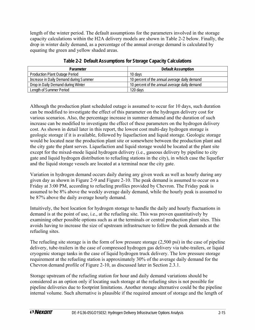
length of the winter period. The default assumptions for the parameters involved in the storage capacity calculations within the H2A delivery models are shown in Table 2-2 below. Finally, the drop in winter daily demand, as a percentage of the annual average demand is calculated by equating the green and yellow shaded areas.
Table 2-2 Default Assumptions for Storage Capacity Calculations Parameter Default Assumption
Production Plant Outage Period 10 days Increase in Daily Demand during Summer 10 percent of the annual average daily demand Drop in Daily Demand during Winter 10 percent of the annual average daily demand Length of Summer Period 120 days
Although the production plant scheduled outage is assumed to occur for 10 days, such duration can be modified to investigate the effect of this parameter on the hydrogen delivery cost for various scenarios. Also, the percentage increase in summer demand and the duration of such increase can be modified to investigate the effect of these parameters on the hydrogen delivery cost. As shown in detail later in this report, the lowest cost multi-day hydrogen storage is geologic storage if it is available, followed by liquefaction and liquid storage. Geologic storage would be located near the production plant site or somewhere between the production plant and the city gate the plant serves. Liquefaction and liquid storage would be located at the plant site except for the mixed-mode liquid hydrogen delivery (i.e., gaseous delivery by pipeline to city gate and liquid hydrogen distribution to refueling stations in the city), in which case the liquefier and the liquid storage vessels are located at a terminal near the city gate.
Variation in hydrogen demand occurs daily during any given week as well as hourly during any given day as shown in Figure 2-9 and Figure 2-10. The peak demand is assumed to occur on a Friday at 3:00 PM, according to refueling profiles provided by Chevron. The Friday peak is assumed to be 8% above the weekly average daily demand, while the hourly peak is assumed to be 87% above the daily average hourly demand.
Intuitively, the best location for hydrogen storage to handle the daily and hourly fluctuations in demand is at the point of use, i.e., at the refueling site. This was proven quantitatively by examining other possible options such as at the terminals or central production plant sites. This avoids having to increase the size of upstream infrastructure to follow the peak demands at the refueling sites.
The refueling site storage is in the form of low pressure storage (2,500 psi) in the case of pipeline delivery, tube-trailers in the case of compressed hydrogen gas delivery via tube-trailers, or liquid cryogenic storage tanks in the case of liquid hydrogen truck delivery. The low pressure storage requirement at the refueling station is approximately 30% of the average daily demand for the Chevron demand profile of Figure 2-10, as discussed later in Section 2.3.1.
Storage upstream of the refueling station for hour and daily demand variations should be considered as an option only if locating such storage at the refueling sites is not possible for pipeline deliveries due to footprint limitations. Another storage alternative could be the pipeline internal volume. Such alternative is plausible if the required amount of storage and the length of
DE-FG36-05GO15032: Hydrogen Delivery Infrastructure Options Analysis 2-15
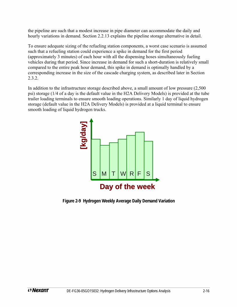
DE-FG36-05GO15032: Hydrogen Delivery Infrastructure Options Analysis 2-16
the pipeline are such that a modest increase in pipe diameter can accommodate the daily and hourly variations in demand. Section 2.2.13 explains the pipeline storage alternative in detail.
To ensure adequate sizing of the refueling station components, a worst case scenario is assumed such that a refueling station could experience a spike in demand for the first period (approximately 3 minutes) of each hour with all the dispensing hoses simultaneously fueling vehicles during that period. Since increase in demand for such a short-duration is relatively small compared to the entire peak hour demand, this spike in demand is optimally handled by a corresponding increase in the size of the cascade charging system, as described later in Section 2.3.2.
In addition to the infrastructure storage described above, a small amount of low pressure (2,500 psi) storage (1/4 of a day is the default value in the H2A Delivery Models) is provided at the tube trailer loading terminals to ensure smooth loading operations. Similarly 1 day of liquid hydrogen storage (default value in the H2A Delivery Models) is provided at a liquid terminal to ensure smooth loading of liquid hydrogen trucks.
[kg/
day]
S M T W R F S
Day of the week
[kg/
day]
S M T W R F SS M T W R F S
Day of the week
Figure 2-9 Hydrogen Weekly Average Daily Demand Variation
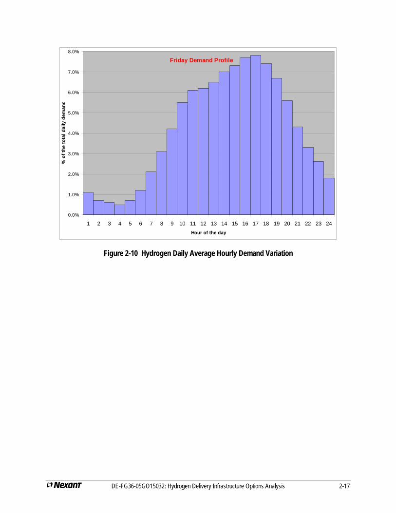
DE-FG36-05GO15032: Hydrogen Delivery Infrastructure Options Analysis 2-17
Friday Demand Profile
0.0%
1.0%
2.0%
3.0%
4.0%
5.0%
6.0%
7.0%
8.0%
1 2 3 4 5 6 7 8 9 10 11 12 13 14 15 16 17 18 19 20 21 22 23 24Hour of the day
% o
f the
tota
l dai
ly d
eman
d
Figure 2-10 Hydrogen Daily Average Hourly Demand Variation
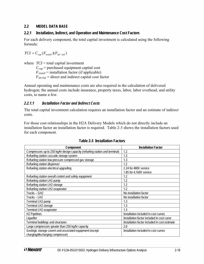
2.2 MODEL DATA BASE 2.2.1 Installation, Indirect, and Operation and Maintenance Cost Factors For each delivery component, the total capital investment is calculated using the following formula:
))(( / inddirinstallcap FFCTCI =
where TCI = total capital investment Ccap = purchased equipment capital cost Finstall = installation factor (if applicable) Fdir/ind = direct and indirect capital cost factor
Annual operating and maintenance costs are also required in the calculation of delivered hydrogen; the annual costs include insurance, property taxes, labor, labor overhead, and utility costs, to name a few.
2.2.1.1 Installation Factor and Indirect Costs The total capital investment calculation requires an installation factor and an estimate of indirect costs.
For those cost relationships in the H2A Delivery Models which do not directly include an installation factor an installation factor is required. Table 2-3 shows the installation factors used for each component.
Table 2-3 Installation Factors Component Installation Factor
Compressors up to 250 kg/hr design capacity (refueling station and terminal) 1.2 Refueling station cascade storage system 1.3 Refueling station low pressure compressed gas storage 1.3 Refueling station dispenser 1.2 Refueling station electrical upgrading 2.24 for 480V service
1.85 for 4,160V service Refueling station overall control and safety equipment 1.2 Refueling station LH2 pump 1.2 Refueling station LH2 storage 1.2 Refueling station LH2 evaporator 1.2 Trucks – GH2 No installation factor Trucks – LH2 No installation factor Terminal LH2 pump 1.3 Terminal LH2 storage 1.3 Terminal LH2 evaporator 1.3 H2 Pipelines Installation included in cost curves Liquefier Installation factor included in cost curve Terminal buildings and structures Installation factor included in cost estimate Large compressors greater than 250 kg/hr capacity 2.0 Geologic storage cavern and associated equipment (except charging/discharging compressor)
Installation included in cost curves
DE-FG36-05GO15032: Hydrogen Delivery Infrastructure Options Analysis 2-18
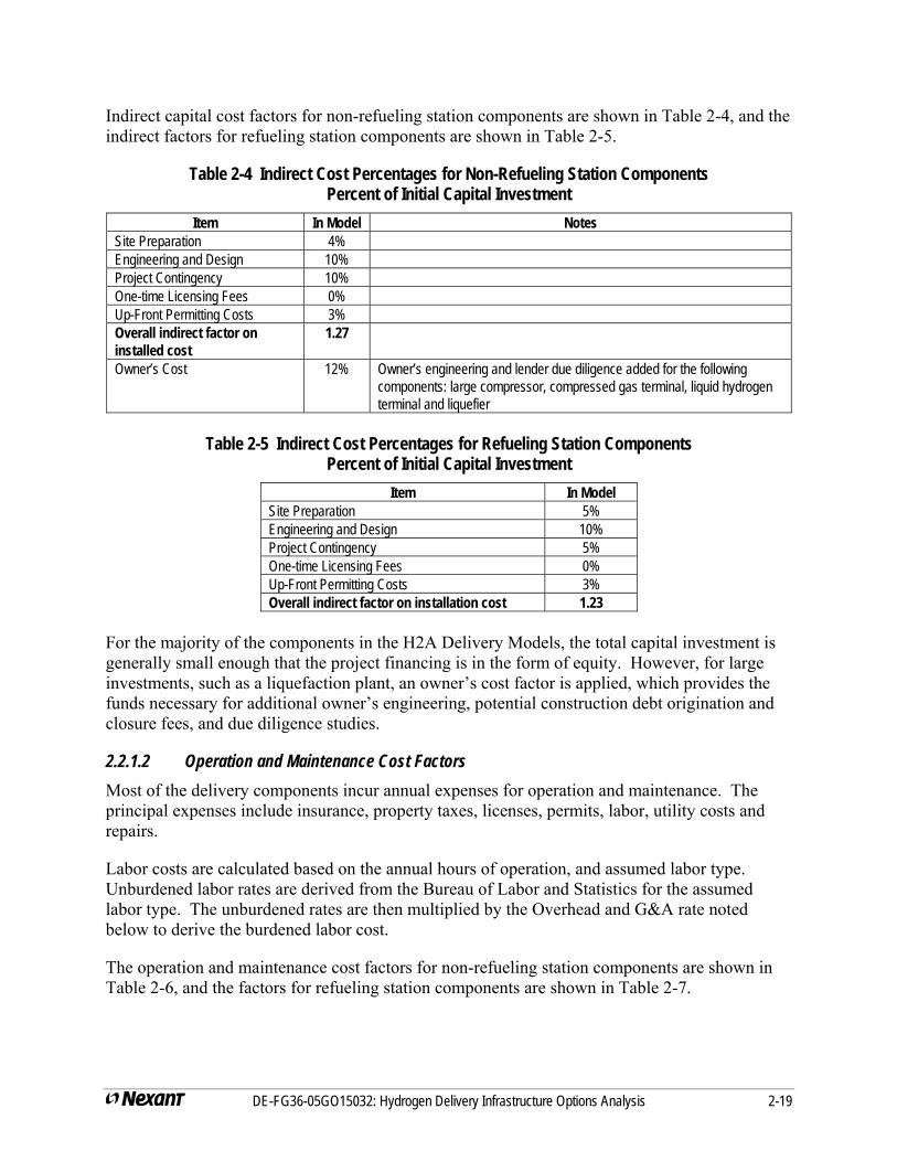
Indirect capital cost factors for non-refueling station components are shown in Table 2-4, and the indirect factors for refueling station components are shown in Table 2-5.
Table 2-4 Indirect Cost Percentages for Non-Refueling Station Components Percent of Initial Capital Investment
Item In Model Notes
Site Preparation 4% Engineering and Design 10% Project Contingency 10% One-time Licensing Fees 0% Up-Front Permitting Costs 3% Overall indirect factor on installed cost
1.27
Owner’s Cost 12% Owner’s engineering and lender due diligence added for the following components: large compressor, compressed gas terminal, liquid hydrogen terminal and liquefier
Table 2-5 Indirect Cost Percentages for Refueling Station Components
Percent of Initial Capital Investment Item In Model
Site Preparation 5% Engineering and Design 10% Project Contingency 5% One-time Licensing Fees 0% Up-Front Permitting Costs 3% Overall indirect factor on installation cost 1.23
For the majority of the components in the H2A Delivery Models, the total capital investment is generally small enough that the project financing is in the form of equity. However, for large investments, such as a liquefaction plant, an owner’s cost factor is applied, which provides the funds necessary for additional owner’s engineering, potential construction debt origination and closure fees, and due diligence studies.
2.2.1.2 Operation and Maintenance Cost Factors Most of the delivery components incur annual expenses for operation and maintenance. The principal expenses include insurance, property taxes, licenses, permits, labor, utility costs and repairs.
Labor costs are calculated based on the annual hours of operation, and assumed labor type. Unburdened labor rates are derived from the Bureau of Labor and Statistics for the assumed labor type. The unburdened rates are then multiplied by the Overhead and G&A rate noted below to derive the burdened labor cost.
The operation and maintenance cost factors for non-refueling station components are shown in Table 2-6, and the factors for refueling station components are shown in Table 2-7.
DE-FG36-05GO15032: Hydrogen Delivery Infrastructure Options Analysis 2-19
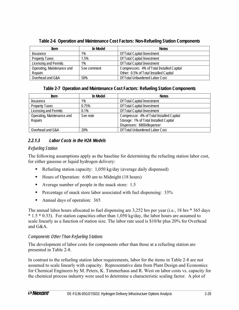
Table 2-6 Operation and Maintenance Cost Factors: Non-Refueling Station Components Item In Model Notes
Insurance 1% Of Total Capital Investment Property Taxes 1.5% Of Total Capital Investment Licensing and Permits 1% Of Total Capital Investment Operating, Maintenance and Repairs
See comment Compressors: 4% of Total Installed Capital Other: 0.5% of Total Installed Capital
Overhead and G&A 50% Of Total Unburdened Labor Cost
Table 2-7 Operation and Maintenance Cost Factors: Refueling Station Components Item In Model Notes
Insurance 1% Of Total Capital Investment Property Taxes 0.75% Of Total Capital Investment Licensing and Permits 0.1% Of Total Capital Investment Operating, Maintenance and Repairs
See note Compressor: 4% of Total Installed Capital Storage: 1% of Total Installed Capital Dispensers: $800/dispenser
Overhead and G&A 20% Of Total Unburdened Labor Cost 2.2.1.3 Labor Costs in the H2A Models Refueling Station The following assumptions apply as the baseline for determining the refueling station labor cost, for either gaseous or liquid hydrogen delivery:
Refueling station capacity: 1,050 kg/day (average daily dispensed)
Hours of Operation: 6:00 am to Midnight (18 hours)
Average number of people in the snack store: 1.5
Percentage of snack store labor associated with fuel dispensing: 33%
Annual days of operation: 365
The annual labor hours allocated to fuel dispensing are 3,252 hrs per year (i.e., 18 hrs * 365 days * 1.5 * 0.33). For station capacities other than 1,050 kg/day, the labor hours are assumed to scale linearly as a function of station size. The labor rate used is $10/hr plus 20% for Overhead and G&A.
Components Other Than Refueling Stations The development of labor costs for components other than those at a refueling station are presented in Table 2-8.
In contrast to the refueling station labor requirements, labor for the items in Table 2-8 are not assumed to scale linearly with capacity. Representative data from Plant Design and Economics for Chemical Engineers by M. Peters, K. Timmerhaus and R. West on labor costs vs. capacity for the chemical process industry were used to determine a characteristic scaling factor. A plot of
DE-FG36-05GO15032: Hydrogen Delivery Infrastructure Options Analysis 2-20
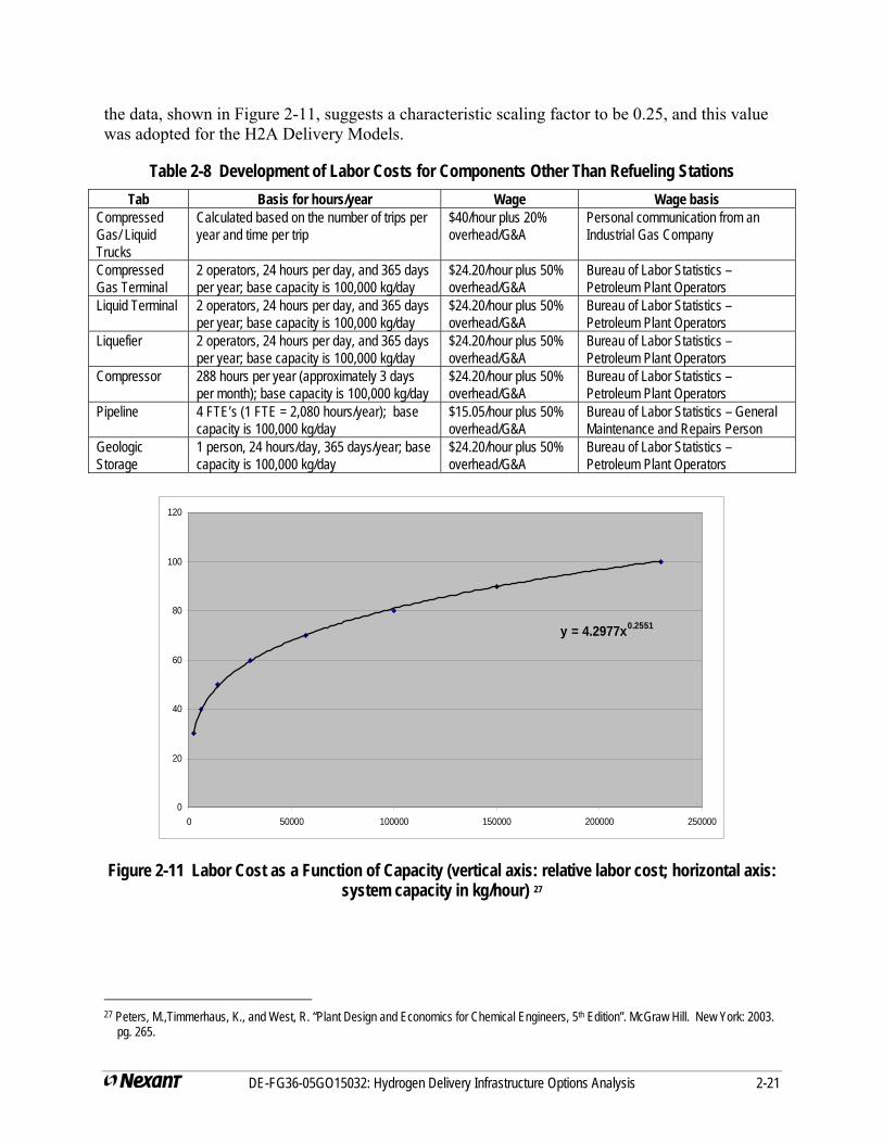
DE-FG36-05GO15032: Hydrogen Delivery Infrastructure Options Analysis 2-21
the data, shown in Figure 2-11, suggests a characteristic scaling factor to be 0.25, and this value was adopted for the H2A Delivery Models.
Table 2-8 Development of Labor Costs for Components Other Than Refueling Stations Tab Basis for hours/year Wage Wage basis
Compressed Gas/ Liquid Trucks
Calculated based on the number of trips per year and time per trip
$40/hour plus 20% overhead/G&A
Personal communication from an Industrial Gas Company
Compressed Gas Terminal
2 operators, 24 hours per day, and 365 days per year; base capacity is 100,000 kg/day
$24.20/hour plus 50% overhead/G&A
Bureau of Labor Statistics – Petroleum Plant Operators
Liquid Terminal 2 operators, 24 hours per day, and 365 days per year; base capacity is 100,000 kg/day
$24.20/hour plus 50% overhead/G&A
Bureau of Labor Statistics – Petroleum Plant Operators
Liquefier 2 operators, 24 hours per day, and 365 days per year; base capacity is 100,000 kg/day
$24.20/hour plus 50% overhead/G&A
Bureau of Labor Statistics – Petroleum Plant Operators
Compressor 288 hours per year (approximately 3 days per month); base capacity is 100,000 kg/day
$24.20/hour plus 50% overhead/G&A
Bureau of Labor Statistics – Petroleum Plant Operators
Pipeline 4 FTE’s (1 FTE = 2,080 hours/year); base capacity is 100,000 kg/day
$15.05/hour plus 50% overhead/G&A
Bureau of Labor Statistics – General Maintenance and Repairs Person
Geologic Storage
1 person, 24 hours/day, 365 days/year; base capacity is 100,000 kg/day
$24.20/hour plus 50% overhead/G&A
Bureau of Labor Statistics – Petroleum Plant Operators
y = 4.2977x0.2551
0
20
40
60
80
100
120
0 50000 100000 150000 200000 250000
Figure 2-11 Labor Cost as a Function of Capacity (vertical axis: relative labor cost; horizontal axis: system capacity in kg/hour) 27
27 Peters, M.,Timmerhaus, K., and West, R. “Plant Design and Economics for Chemical Engineers, 5th Edition”. McGraw Hill. New York: 2003.
pg. 265.
DE-FG36-05GO15032: Hydrogen Delivery Infrastructure Options Analysis 2-22
2.2.2 Hydrogen Pipeline Costs 2.2.2.1 Transmission Pipeline Costs Equations for estimating transmission pipeline costs were developed from historical cost data for natural gas transmission lines. Nathan Parker, a graduate student at the University of California at Davis, completed a regression analysis of 13 years of natural gas pipeline data from the Oil and Gas Journal. The equations from Mr. Parker’s report, which are used in the delivery models, are shown below28:
Pipeline materials: (330.5 * (Diameter, in.)2 + 687 * (Diameter, in.) + 26,960)) * (Length, miles) + 35,000
Miscellaneous costs: (8,417 * (Diameter, in.) + 7,324) * (Length, miles) + 95,000
Labor costs: (343 * (Diameter, in.)2 + 2,074 * (Diameter, in.) + 170,013)) * (Length, miles) + 185,000
Right of way: (577 * (Diameter, in.) + 29,788)) * (Length, miles) + 40,000
In the models, each of the equations listed above are multiplied by a factor of 1.1. This factor adjusts the natural gas pipeline costs for higher costs anticipated in a hydrogen pipeline. The increased costs are due to 1) more stringent inspections of the welds, and 2) leak-free seals on the isolation and control valves. This is based on discussions with Industrial Gas companies who build and operate the existing hydrogen pipelines in the U.S. The above equations are also multiplied by 110.5/100 (ratio of GDP indices for 2005 and 2000) in the models to adjust the price year of the original equations (2000) to a price year of 2005.
The pipeline diameter is calculated from the ‘Panhandle B’ equation, which uses a series of parameters to simulate turbulent compressible gas flow in long pipelines29.
2.2.2.2 Distribution Pipeline Costs In the H2A Delivery Component and the Scenario Models V1, unit costs for distribution pipelines within a city were estimated using natural gas pipeline cost equations derived by Nathan Parker at the University of California as explained in Section 2.2.2.1. However, a refinement to this cost approach is desirable. The Oil and Gas natural gas pipeline data are dominated by more rural and larger pipeline diameters and operating pressures higher than are typically used for urban distribution.
During the course of the study, cost information on natural gas distribution line costs were obtained from 4 disparate sources as discussed below. In support of revised cost equations for the H2A Delivery Models, unit distribution pipelines costs for urban and downtown installations were assembled, and plotted as functions of the pipe diameter. Polynomial curve fits were then developed for use in the H2A Delivery Models. For the purposes of the model, the distribution pipelines were assumed to be steel, rather than plastic pipe, as would be appropriate for hydrogen pipelines. As a result, the cost analyses were based exclusively on steel pipeline data.
28 Parker, Nathan. "Using Natural Gas Transmission Pipeline Costs to Estimate Hydrogen Pipeline Costs," Technical Report No. UCD-ITS-RR-
04-3, Institute of Transportation Studies, University of California, Davis, January 2005. 29 Gas Processors Supplier Association, Engineering Data Book, 11th Edition, 1998, http://gpsa.gasprocessors.com
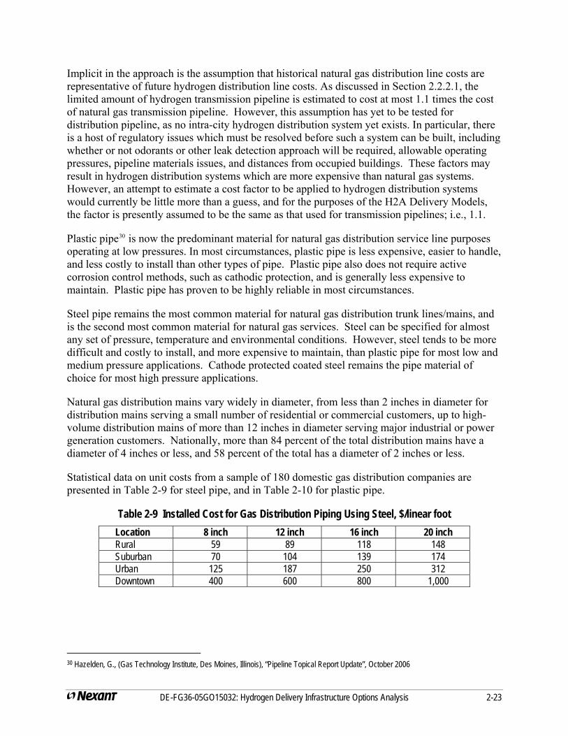
DE-FG36-05GO15032: Hydrogen Delivery Infrastructure Options Analysis 2-23
Implicit in the approach is the assumption that historical natural gas distribution line costs are representative of future hydrogen distribution line costs. As discussed in Section 2.2.2.1, the limited amount of hydrogen transmission pipeline is estimated to cost at most 1.1 times the cost of natural gas transmission pipeline. However, this assumption has yet to be tested for distribution pipeline, as no intra-city hydrogen distribution system yet exists. In particular, there is a host of regulatory issues which must be resolved before such a system can be built, including whether or not odorants or other leak detection approach will be required, allowable operating pressures, pipeline materials issues, and distances from occupied buildings. These factors may result in hydrogen distribution systems which are more expensive than natural gas systems. However, an attempt to estimate a cost factor to be applied to hydrogen distribution systems would currently be little more than a guess, and for the purposes of the H2A Delivery Models, the factor is presently assumed to be the same as that used for transmission pipelines; i.e., 1.1.
Plastic pipe30 is now the predominant material for natural gas distribution service line purposes operating at low pressures. In most circumstances, plastic pipe is less expensive, easier to handle, and less costly to install than other types of pipe. Plastic pipe also does not require active corrosion control methods, such as cathodic protection, and is generally less expensive to maintain. Plastic pipe has proven to be highly reliable in most circumstances.
Steel pipe remains the most common material for natural gas distribution trunk lines/mains, and is the second most common material for natural gas services. Steel can be specified for almost any set of pressure, temperature and environmental conditions. However, steel tends to be more difficult and costly to install, and more expensive to maintain, than plastic pipe for most low and medium pressure applications. Cathode protected coated steel remains the pipe material of choice for most high pressure applications.
Natural gas distribution mains vary widely in diameter, from less than 2 inches in diameter for distribution mains serving a small number of residential or commercial customers, up to high-volume distribution mains of more than 12 inches in diameter serving major industrial or power generation customers. Nationally, more than 84 percent of the total distribution mains have a diameter of 4 inches or less, and 58 percent of the total has a diameter of 2 inches or less.
Statistical data on unit costs from a sample of 180 domestic gas distribution companies are presented in Table 2-9 for steel pipe, and in Table 2-10 for plastic pipe.
Table 2-9 Installed Cost for Gas Distribution Piping Using Steel, $/linear foot Location 8 inch 12 inch 16 inch 20 inch Rural 59 89 118 148 Suburban 70 104 139 174 Urban 125 187 250 312 Downtown 400 600 800 1,000
30 Hazelden, G., (Gas Technology Institute, Des Moines, Illinois), “Pipeline Topical Report Update”, October 2006
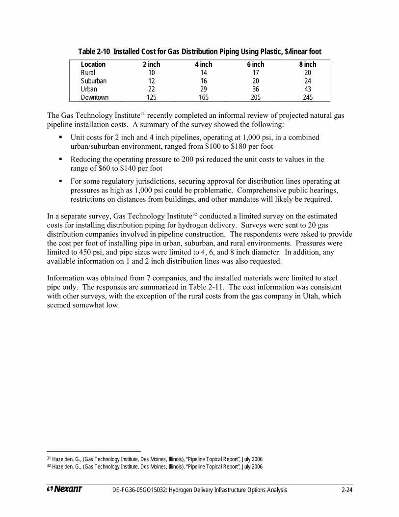
DE-FG36-05GO15032: Hydrogen Delivery Infrastructure Options Analysis 2-24
Table 2-10 Installed Cost for Gas Distribution Piping Using Plastic, $/linear foot Location 2 inch 4 inch 6 inch 8 inch Rural 10 14 17 20 Suburban 12 16 20 24 Urban 22 29 36 43 Downtown 125 165 205 245
The Gas Technology Institute31 recently completed an informal review of projected natural gas pipeline installation costs. A summary of the survey showed the following:
Unit costs for 2 inch and 4 inch pipelines, operating at 1,000 psi, in a combined urban/suburban environment, ranged from $100 to $180 per foot
Reducing the operating pressure to 200 psi reduced the unit costs to values in the range of $60 to $140 per foot
For some regulatory jurisdictions, securing approval for distribution lines operating at pressures as high as 1,000 psi could be problematic. Comprehensive public hearings, restrictions on distances from buildings, and other mandates will likely be required.
In a separate survey, Gas Technology Institute32 conducted a limited survey on the estimated costs for installing distribution piping for hydrogen delivery. Surveys were sent to 20 gas distribution companies involved in pipeline construction. The respondents were asked to provide the cost per foot of installing pipe in urban, suburban, and rural environments. Pressures were limited to 450 psi, and pipe sizes were limited to 4, 6, and 8 inch diameter. In addition, any available information on 1 and 2 inch distribution lines was also requested.
Information was obtained from 7 companies, and the installed materials were limited to steel pipe only. The responses are summarized in Table 2-11. The cost information was consistent with other surveys, with the exception of the rural costs from the gas company in Utah, which seemed somewhat low.
31 Hazelden, G., (Gas Technology Institute, Des Moines, Illinois), “Pipeline Topical Report”, July 2006 32 Hazelden, G., (Gas Technology Institute, Des Moines, Illinois), “Pipeline Topical Report”, July 2006
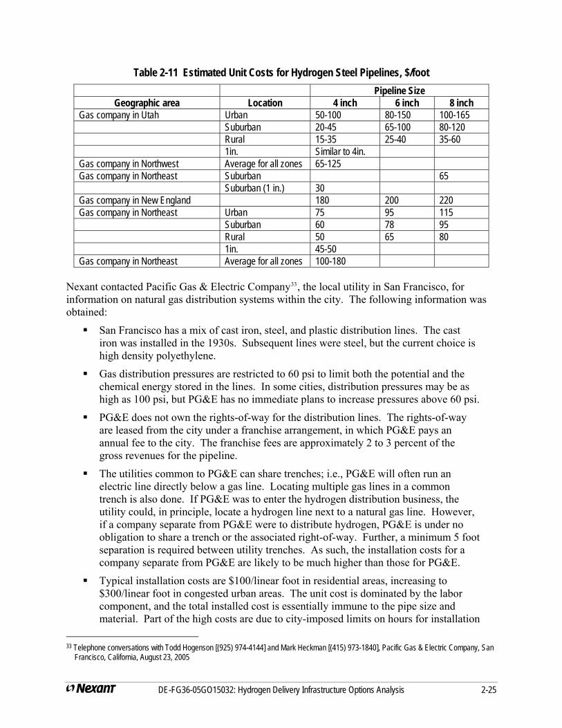
DE-FG36-05GO15032: Hydrogen Delivery Infrastructure Options Analysis 2-25
Table 2-11 Estimated Unit Costs for Hydrogen Steel Pipelines, $/foot Pipeline Size
Geographic area Location 4 inch 6 inch 8 inch Gas company in Utah Urban 50-100 80-150 100-165 Suburban 20-45 65-100 80-120 Rural 15-35 25-40 35-60 1in. Similar to 4in. Gas company in Northwest Average for all zones 65-125 Gas company in Northeast Suburban 65 Suburban (1 in.) 30 Gas company in New England 180 200 220 Gas company in Northeast Urban 75 95 115 Suburban 60 78 95 Rural 50 65 80 1in. 45-50 Gas company in Northeast Average for all zones 100-180
Nexant contacted Pacific Gas & Electric Company33, the local utility in San Francisco, for information on natural gas distribution systems within the city. The following information was obtained:
San Francisco has a mix of cast iron, steel, and plastic distribution lines. The cast iron was installed in the 1930s. Subsequent lines were steel, but the current choice is high density polyethylene.
Gas distribution pressures are restricted to 60 psi to limit both the potential and the chemical energy stored in the lines. In some cities, distribution pressures may be as high as 100 psi, but PG&E has no immediate plans to increase pressures above 60 psi.
PG&E does not own the rights-of-way for the distribution lines. The rights-of-way are leased from the city under a franchise arrangement, in which PG&E pays an annual fee to the city. The franchise fees are approximately 2 to 3 percent of the gross revenues for the pipeline.
The utilities common to PG&E can share trenches; i.e., PG&E will often run an electric line directly below a gas line. Locating multiple gas lines in a common trench is also done. If PG&E was to enter the hydrogen distribution business, the utility could, in principle, locate a hydrogen line next to a natural gas line. However, if a company separate from PG&E were to distribute hydrogen, PG&E is under no obligation to share a trench or the associated right-of-way. Further, a minimum 5 foot separation is required between utility trenches. As such, the installation costs for a company separate from PG&E are likely to be much higher than those for PG&E.
Typical installation costs are $100/linear foot in residential areas, increasing to $300/linear foot in congested urban areas. The unit cost is dominated by the labor component, and the total installed cost is essentially immune to the pipe size and material. Part of the high costs are due to city-imposed limits on hours for installation
33 Telephone conversations with Todd Hogenson [(925) 974-4144] and Mark Heckman [(415) 973-1840], Pacific Gas & Electric Company, San
Francisco, California, August 23, 2005
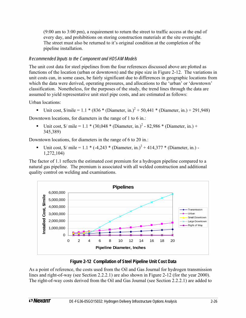
(9:00 am to 3:00 pm), a requirement to return the street to traffic access at the end of every day, and prohibitions on storing construction materials at the site overnight. The street must also be returned to it’s original condition at the completion of the pipeline installation.
Recommended Inputs to the Component and HDSAM Models The unit cost data for steel pipelines from the four references discussed above are plotted as functions of the location (urban or downtown) and the pipe size in Figure 2-12. The variations in unit costs can, in some cases, be fairly significant due to differences in geographic locations from which the data were derived, operating pressures, and allocations to the ‘urban’ or ‘downtown’ classification. Nonetheless, for the purposes of the study, the trend lines through the data are assumed to yield representative unit steel pipe costs, and are estimated as follows:
Urban locations:
Unit cost, $/mile = 1.1 * (836 * (Diameter, in.)2 + 50,441 * (Diameter, in.) + 291,948)
Downtown locations, for diameters in the range of 1 to 6 in.:
Unit cost, $/ mile = 1.1 * (30,048 * (Diameter, in.)2 - 82,986 * (Diameter, in.) + 345,389)
Downtown locations, for diameters in the range of 6 to 20 in.:
Unit cost, $/ mile = 1.1 * (-4,243 * (Diameter, in.)2 + 414,377 * (Diameter, in.) - 1,272,104)
The factor of 1.1 reflects the estimated cost premium for a hydrogen pipeline compared to a natural gas pipeline. The premium is associated with all welded construction and additional quality control on welding and examinations.
Pipelines
0
1,000,000
2,000,000
3,000,000
4,000,000
5,000,000
6,000,000
0 2 4 6 8 10 12 14 16 18 20
Pipeline Diameter, Inches
Inst
alle
d Co
st, $
/mile
TransmissionUrbanSmall DowntownLarge DowntownRight of Way
Figure 2-12 Compilation of Steel Pipeline Unit Cost Data
As a point of reference, the costs used from the Oil and Gas Journal for hydrogen transmission lines and right-of-way (see Section 2.2.2.1) are also shown in Figure 2-12 (for the year 2000). The right-of-way costs derived from the Oil and Gas Journal (see Section 2.2.2.1) are added to
DE-FG36-05GO15032: Hydrogen Delivery Infrastructure Options Analysis 2-26
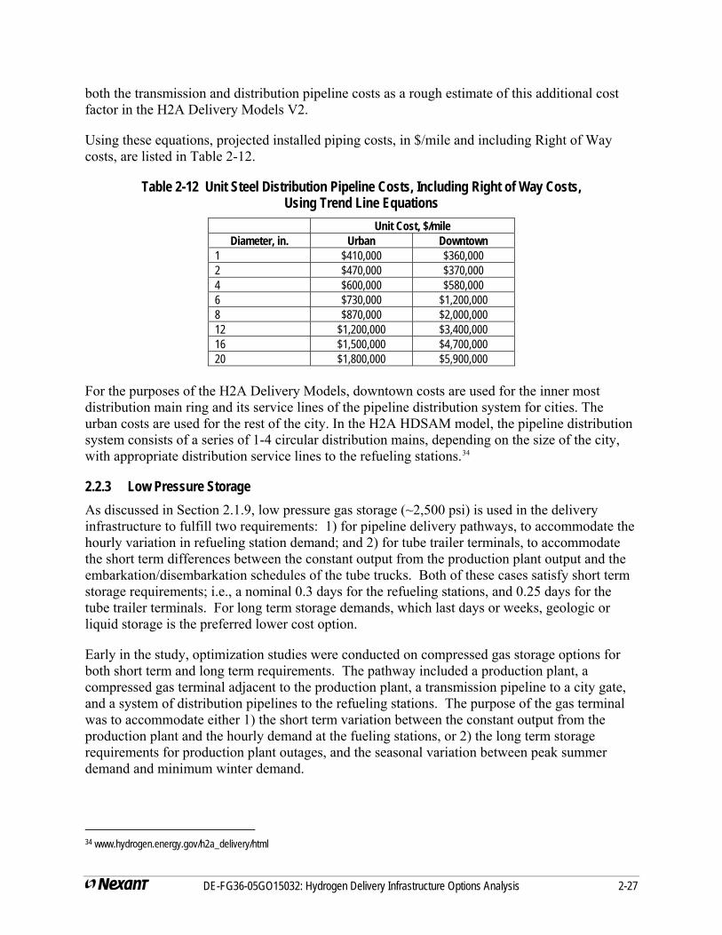
DE-FG36-05GO15032: Hydrogen Delivery Infrastructure Options Analysis 2-27
both the transmission and distribution pipeline costs as a rough estimate of this additional cost factor in the H2A Delivery Models V2.
Using these equations, projected installed piping costs, in $/mile and including Right of Way costs, are listed in Table 2-12.
Table 2-12 Unit Steel Distribution Pipeline Costs, Including Right of Way Costs, Using Trend Line Equations
Unit Cost, $/mile Diameter, in. Urban Downtown
1 $410,000 $360,000 2 $470,000 $370,000 4 $600,000 $580,000 6 $730,000 $1,200,000 8 $870,000 $2,000,000 12 $1,200,000 $3,400,000 16 $1,500,000 $4,700,000 20 $1,800,000 $5,900,000
For the purposes of the H2A Delivery Models, downtown costs are used for the inner most distribution main ring and its service lines of the pipeline distribution system for cities. The urban costs are used for the rest of the city. In the H2A HDSAM model, the pipeline distribution system consists of a series of 1-4 circular distribution mains, depending on the size of the city, with appropriate distribution service lines to the refueling stations.34
2.2.3 Low Pressure Storage As discussed in Section 2.1.9, low pressure gas storage (~2,500 psi) is used in the delivery infrastructure to fulfill two requirements: 1) for pipeline delivery pathways, to accommodate the hourly variation in refueling station demand; and 2) for tube trailer terminals, to accommodate the short term differences between the constant output from the production plant output and the embarkation/disembarkation schedules of the tube trucks. Both of these cases satisfy short term storage requirements; i.e., a nominal 0.3 days for the refueling stations, and 0.25 days for the tube trailer terminals. For long term storage demands, which last days or weeks, geologic or liquid storage is the preferred lower cost option.
Early in the study, optimization studies were conducted on compressed gas storage options for both short term and long term requirements. The pathway included a production plant, a compressed gas terminal adjacent to the production plant, a transmission pipeline to a city gate, and a system of distribution pipelines to the refueling stations. The purpose of the gas terminal was to accommodate either 1) the short term variation between the constant output from the production plant and the hourly demand at the fueling stations, or 2) the long term storage requirements for production plant outages, and the seasonal variation between peak summer demand and minimum winter demand.
34 www.hydrogen.energy.gov/h2a_delivery/html
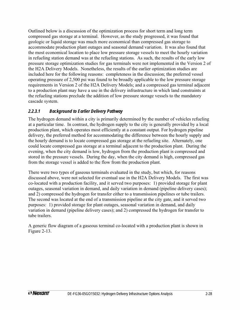
Outlined below is a discussion of the optimization process for short term and long term compressed gas storage at a terminal. However, as the study progressed, it was found that geologic or liquid storage was much more economical than compressed gas storage to accommodate production plant outages and seasonal demand variation. It was also found that the most economical location to place low pressure storage vessels to meet the hourly variation in refueling station demand was at the refueling stations. As such, the results of the early low pressure storage optimization studies for gas terminals were not implemented in the Version 2 of the H2A Delivery Models. Nonetheless, the results of the earlier optimization studies are included here for the following reasons: completeness in the discussion; the preferred vessel operating pressure of 2,500 psi was found to be broadly applicable to the low pressure storage requirements in Version 2 of the H2A Delivery Models; and a compressed gas terminal adjacent to a production plant may have a use in the delivery infrastructure in which land constraints at the refueling stations preclude the addition of low pressure storage vessels to the mandatory cascade system.
2.2.3.1 Background to Earlier Delivery Pathway The hydrogen demand within a city is primarily determined by the number of vehicles refueling at a particular time. In contrast, the hydrogen supply to the city is generally provided by a local production plant, which operates most efficiently at a constant output. For hydrogen pipeline delivery, the preferred method for accommodating the difference between the hourly supply and the hourly demand is to locate compressed gas storage at the refueling site. Alternately, one could locate compressed gas storage at a terminal adjacent to the production plant. During the evening, when the city demand is low, hydrogen from the production plant is compressed and stored in the pressure vessels. During the day, when the city demand is high, compressed gas from the storage vessel is added to the flow from the production plant.
There were two types of gaseous terminals evaluated in the study, but which, for reasons discussed above, were not selected for eventual use in the H2A Delivery Models. The first was co-located with a production facility, and it served two purposes: 1) provided storage for plant outages, seasonal variation in demand, and daily variation in demand (pipeline delivery cases); and 2) compressed the hydrogen for transfer either to a transmission pipelines or tube trailers. The second was located at the end of a transmission pipeline at the city gate, and it served two purposes: 1) provided storage for plant outages, seasonal variation in demand, and daily variation in demand (pipeline delivery cases); and 2) compressed the hydrogen for transfer to tube trailers.
A generic flow diagram of a gaseous terminal co-located with a production plant is shown in Figure 2-13.
DE-FG36-05GO15032: Hydrogen Delivery Infrastructure Options Analysis 2-28
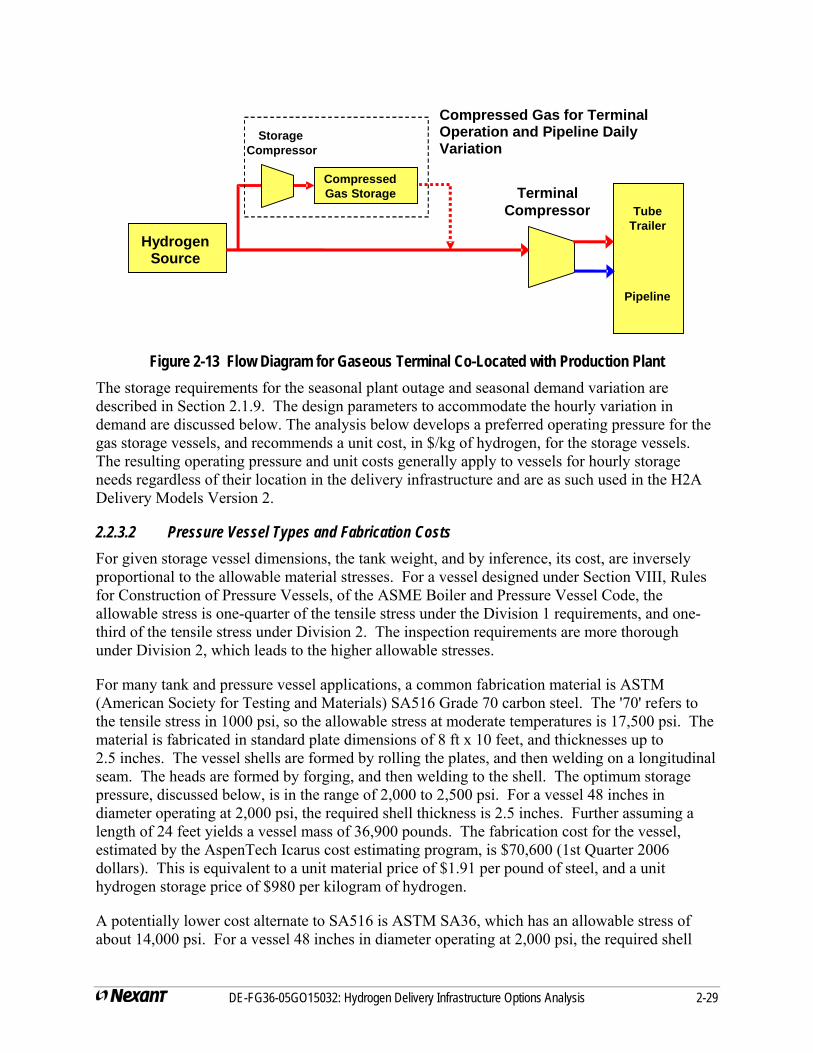
Hydrogen Source
Compressed Gas Storage
Tube Trailer
Pipeline
Storage Compressor
Compressed Gas for Terminal Operation and Pipeline Daily Variation
Terminal Compressor
Figure 2-13 Flow Diagram for Gaseous Terminal Co-Located with Production Plant
The storage requirements for the seasonal plant outage and seasonal demand variation are described in Section 2.1.9. The design parameters to accommodate the hourly variation in demand are discussed below. The analysis below develops a preferred operating pressure for the gas storage vessels, and recommends a unit cost, in $/kg of hydrogen, for the storage vessels. The resulting operating pressure and unit costs generally apply to vessels for hourly storage needs regardless of their location in the delivery infrastructure and are as such used in the H2A Delivery Models Version 2.
2.2.3.2 Pressure Vessel Types and Fabrication Costs For given storage vessel dimensions, the tank weight, and by inference, its cost, are inversely proportional to the allowable material stresses. For a vessel designed under Section VIII, Rules for Construction of Pressure Vessels, of the ASME Boiler and Pressure Vessel Code, the allowable stress is one-quarter of the tensile stress under the Division 1 requirements, and one-third of the tensile stress under Division 2. The inspection requirements are more thorough under Division 2, which leads to the higher allowable stresses.
For many tank and pressure vessel applications, a common fabrication material is ASTM (American Society for Testing and Materials) SA516 Grade 70 carbon steel. The '70' refers to the tensile stress in 1000 psi, so the allowable stress at moderate temperatures is 17,500 psi. The material is fabricated in standard plate dimensions of 8 ft x 10 feet, and thicknesses up to 2.5 inches. The vessel shells are formed by rolling the plates, and then welding on a longitudinal seam. The heads are formed by forging, and then welding to the shell. The optimum storage pressure, discussed below, is in the range of 2,000 to 2,500 psi. For a vessel 48 inches in diameter operating at 2,000 psi, the required shell thickness is 2.5 inches. Further assuming a length of 24 feet yields a vessel mass of 36,900 pounds. The fabrication cost for the vessel, estimated by the AspenTech Icarus cost estimating program, is $70,600 (1st Quarter 2006 dollars). This is equivalent to a unit material price of $1.91 per pound of steel, and a unit hydrogen storage price of $980 per kilogram of hydrogen.
A potentially lower cost alternate to SA516 is ASTM SA36, which has an allowable stress of about 14,000 psi. For a vessel 48 inches in diameter operating at 2,000 psi, the required shell
DE-FG36-05GO15032: Hydrogen Delivery Infrastructure Options Analysis 2-29
DE-FG36-05GO15032: Hydrogen Delivery Infrastructure Options Analysis 2-30
thickness would be 3.25 inches. Further assuming a length of 24 feet yields a vessel mass of 46,300 pounds. With this design, the estimated cost using the Icarus program is $82,500. This is equivalent to a unit material price of $1.78 per pound of steel, which is a savings of 7 percent compared to SA516. However, the thicker wall thickness reduces the inside diameter, which leads to an increase in the unit hydrogen storage price to $1,223 per kilogram.
In the South Coast Air Quality Management District report "Status Report for Hydrogen Study Team", CP Industries provided a quote on 3 of their ASME vessels35. The vessels start as seamless pipe, and the heads are formed by heating and forging each end of the pipe; there is no longitudinal or circumferential welding involved. The material is ASTM SA372, Grade J, Class 70, with a tensile stress of 120,000 psi. For Division 2 fabrication, the allowable stress is 40,000 psi, or 130 percent higher than SA516. The SCAQMD design is based on the following: 5,500 psi; 20 inches outside diameter; and 22 feet vessel length. Using their quoted FOB price of $56,200 (1st Quarter 2006 dollars) yields a unit material price of $2.75 per pound of steel, and a unit hydrogen storage price of $718 per kilogram of hydrogen.
If the CP Industries approach to vessel fabrication is applied to the requirements of a gas storage vessel, their standard vessel which comes closest in design parameters would be as follows: 2,800 psi design pressure; 24 inch outside diameter; and 25 foot vessel length. Assuming a unit material price of $2.75 per pound of steel results in a unit hydrogen storage price of $596 per kilogram.
Some observations can be made from the above figures:
1) The incremental costs of the high strength steels, in $/lb, compared to the more common carbon steels are small enough that the high strength steels are likely the economic choice for a pressure vessel.
2) Lower storage pressures are preferred. The pressure vessel wall thickness is proportional to the design pressure; however, the stored mass is proportional to the design pressure times the inverse of the compressibility factor. In effect, the inverse of the compressibility factor is equivalent to a storage efficiency, in pounds of gas stored per psi of design pressure. The effect is plotted in Figure 2-14.
35 “Status Report for Hydrogen Study Team, Attachment A, Hydrogen Compatibility Study Team Report and Supporting Documents”, South
Coast Air Quality Management District, August 2001
0.60
0.65
0.70
0.75
0.80
0.85
0.90
0.95
1.00
1.05
0 2,000 4,000 6,000 8,000 10,000 12,000
Hydrogen pressure, psia
1/C
ompr
essi
bilit
y fa
ctor
Figure 2-14 Inverse of Hydrogen Compressibility Factor as a Function of Pressure 3) The vessel fabrication approach adopted by CP Industries is limited to a maximum vessel diameter of 24 inches. 24 inch pipe is available in wall thicknesses up to Schedule 160 (2.344 inches wall thickness), which implies a maximum design pressure on the order of 8,600 psi. However, for pipe diameters of 26 inches and above, the standard wall thicknesses are in the range of 0.5 to 0.75 inches, which effectively limits design pressures to the range of 1,500 to 1,800 psi.
2.2.3.3 Preferred Gas Storage Vessel Operating Pressure The preferred operating pressure for the gas storage at a terminal should be the one which minimizes the sum of the capital cost of the pressure vessel, the capital cost of the compressor, and the equivalent capital cost for the energy supplied to the compressor. The example chosen to examine to quantify these relationships was with the gas storage located at a terminal adjacent to the production plant. To help define the preferred pressure, an Excel spreadsheet model was developed, which calculated each of the above costs over the following ranges of design conditions:
Production plant capacities of 1,000 kg/day, 10,000 kg/day, 325,000 kg/day, 500,000 kg/day, and 800,000 kg/day
Gas storage operating pressures of 1,265 psi to 4,015 psi, in increments of 250 psi.
The pressure vessel dimensions and costs were developed as follows:
The hourly gas flows to, and from, the gas terminal were defined by the difference between the uniform gas delivery from the production plant and the variable demand on the transmission pipeline; the latter was defined by the Chevron gas station fueling profile (see Section 2.1.4). An example of the operating profile for the gas terminal is
DE-FG36-05GO15032: Hydrogen Delivery Infrastructure Options Analysis 2-31
shown in Table 2-13. Positive compression rates represent gas flows from the production plant into storage, and negative compression rates represent gas flows from storage into the transmission pipeline.
Pressure vessel dimensions, wall thicknesses, and weights were calculated using standard formulas, subject to the following constraints: a length-to-diameter ratio not to exceed 6; and a wall thickness not to exceed 2.5 inches.
Unit vessel costs were estimated to be $2.90 per pound, including fabrication, delivery, and sales tax. To this unit price was added 20 percent for the following: steel support frame; concrete foundations; pressure relief valves; inter-vessel piping; isolation valves; installation; and hydraulic test of completed assembly.
Gas terminal compressor capacities and costs were developed as follows:
The design power demand was defined by the following: the highest hourly flow rate to storage from the calculations of the pressure vessel capacities; a 3-stage reciprocating compressor with inter-cooling; and an isentropic compressor efficiency of 88 percent. The maximum compressor capacity was fixed at 16,000 kWe; for higher power levels, multiple compressors were used.
Compressor capital costs were calculated using the cost information presented in Section 2.2.5.
The power to drive the compressor was assumed to be proportional to the hourly hydrogen flow rate into storage; i.e., the compressors were driven by variable speed electric motors, and the efficiency was independent of the compressor speed. The hourly compressor power demands are shown in the last column of Table 2-13.
The annual electric energy cost for the compressors was calculated as follows: (Daily energy demand, kWhe) x (365 days per year) x ($0.065/kWhe for commercial electric energy). The annual energy cost was converted to an equivalent capital cost by dividing the energy cost by a fixed charge rate of 0.15.
The sums of the cost elements are plotted as a function of the storage pressure and the production plant capacity, as shown in Figure 2-15.
DE-FG36-05GO15032: Hydrogen Delivery Infrastructure Options Analysis 2-32
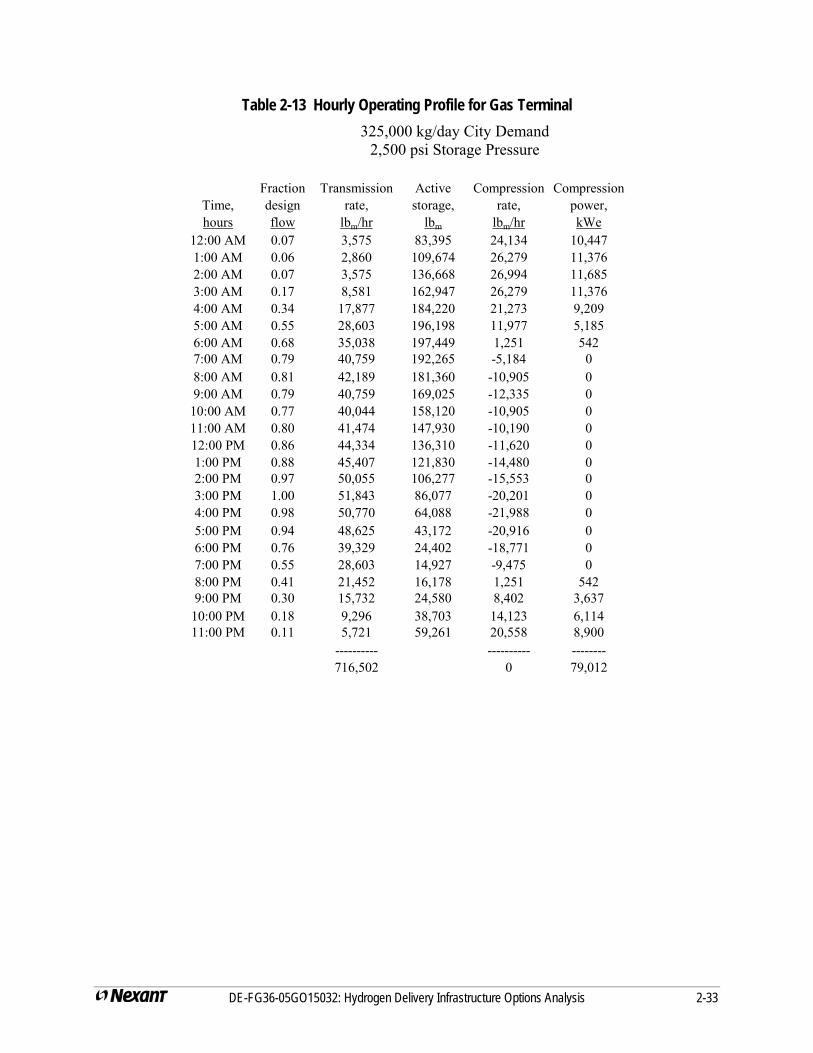
Table 2-13 Hourly Operating Profile for Gas Terminal 325,000 kg/day City Demand
2,500 psi Storage Pressure
Fraction Transmission Active Compression CompressionTime, design rate, storage, rate, power,hours flow lbm/hr lbm lbm/hr kWe
12:00 AM 0.07 3,575 83,395 24,134 10,4471:00 AM 0.06 2,860 109,674 26,279 11,3762:00 AM 0.07 3,575 136,668 26,994 11,6853:00 AM 0.17 8,581 162,947 26,279 11,3764:00 AM 0.34 17,877 184,220 21,273 9,2095:00 AM 0.55 28,603 196,198 11,977 5,1856:00 AM 0.68 35,038 197,449 1,251 5427:00 AM 0.79 40,759 192,265 -5,184 08:00 AM 0.81 42,189 181,360 -10,905 09:00 AM 0.79 40,759 169,025 -12,335 010:00 AM 0.77 40,044 158,120 -10,905 011:00 AM 0.80 41,474 147,930 -10,190 012:00 PM 0.86 44,334 136,310 -11,620 01:00 PM 0.88 45,407 121,830 -14,480 02:00 PM 0.97 50,055 106,277 -15,553 03:00 PM 1.00 51,843 86,077 -20,201 04:00 PM 0.98 50,770 64,088 -21,988 05:00 PM 0.94 48,625 43,172 -20,916 06:00 PM 0.76 39,329 24,402 -18,771 07:00 PM 0.55 28,603 14,927 -9,475 08:00 PM 0.41 21,452 16,178 1,251 5429:00 PM 0.30 15,732 24,580 8,402 3,637
10:00 PM 0.18 9,296 38,703 14,123 6,11411:00 PM 0.11 5,721 59,261 20,558 8,900
---------- ---------- --------716,502 0 79,012
DE-FG36-05GO15032: Hydrogen Delivery Infrastructure Options Analysis 2-33
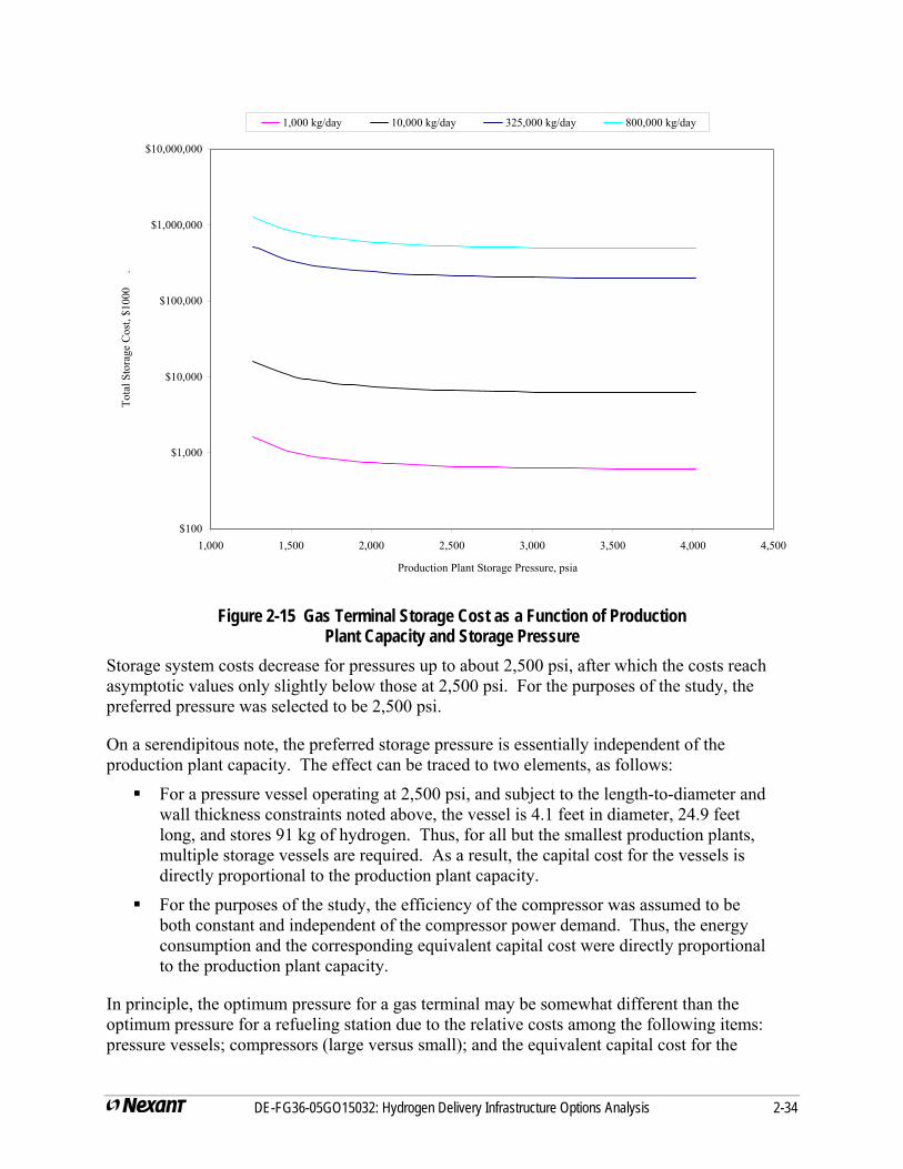
$100
$1,000
$10,000
$100,000
$1,000,000
$10,000,000
1,000 1,500 2,000 2,500 3,000 3,500 4,000 4,500
Production Plant Storage Pressure, psia
Tota
l Sto
rage
Cos
t, $1
000
.
1,000 kg/day 10,000 kg/day 325,000 kg/day 800,000 kg/day
Figure 2-15 Gas Terminal Storage Cost as a Function of Production Plant Capacity and Storage Pressure
Storage system costs decrease for pressures up to about 2,500 psi, after which the costs reach asymptotic values only slightly below those at 2,500 psi. For the purposes of the study, the preferred pressure was selected to be 2,500 psi.
On a serendipitous note, the preferred storage pressure is essentially independent of the production plant capacity. The effect can be traced to two elements, as follows:
For a pressure vessel operating at 2,500 psi, and subject to the length-to-diameter and wall thickness constraints noted above, the vessel is 4.1 feet in diameter, 24.9 feet long, and stores 91 kg of hydrogen. Thus, for all but the smallest production plants, multiple storage vessels are required. As a result, the capital cost for the vessels is directly proportional to the production plant capacity.
For the purposes of the study, the efficiency of the compressor was assumed to be both constant and independent of the compressor power demand. Thus, the energy consumption and the corresponding equivalent capital cost were directly proportional to the production plant capacity.
In principle, the optimum pressure for a gas terminal may be somewhat different than the optimum pressure for a refueling station due to the relative costs among the following items: pressure vessels; compressors (large versus small); and the equivalent capital cost for the
DE-FG36-05GO15032: Hydrogen Delivery Infrastructure Options Analysis 2-34
compressor energy (88 percent isentropic efficiency for large units, versus 65 percent for small). To this end, a series of pressure optimization calculations were developed as above, but substituting refueling station compressor characteristics for gas terminal compressor characteristics. The results showed an optimum pressure of 1,750 psi; however, the total cost for a 2,500 psi design was only 2.5 percent higher than for the 1,750 psi design. For the purposes of the H2A Delivery Models, an optimum low pressure storage pressure of 2,500 psi was selected for all storage requirements, and the associated infrastructure system costs should be nominally representative of a fully optimized design.
2.2.3.4 Design Parameters for Daily Storage As noted in the above, the preferred pressure for low pressure storage is 2,500 psi. However, the calculations did not specify the preferred gas terminal capacity as a function of the city demand, the gas terminal compressor capacity, or the gas terminal compressor annual energy demands for this particular pathway approach. As such, this section addresses the following:
Chevron gas station profile of hourly fuel demand
Gas terminal storage model
Modifications to the Chevron profile due to refueling station equipment capacities
Preferred capacities for the gas terminal, the refueling station compressor, the refueling station cascade charging system.
Chevron Profile Chevron provided the project with fuel dispensing data from gas stations. The data include the following:
Chevron average gasoline station dispenses approximately 4,400 gallons per day, or about 135,000 gallons per month. Assuming a typical fill of 10 to 12 gallons per vehicle, 365 to 440 vehicles visit the gas station on an average day.
The profile of sales by the hour of day reflects the influence of commuter patterns of fueling, mainly on the way to and from work. Figure 2-16 shows the hourly variation in sales on Monday, which has the lowest demand during the week, and Friday, which has the highest. The daily profile shows demand generally increasing around 5:00 am, building through the day, and reaching a maximum in the middle of the afternoon.
For the delivery infrastructure study, the principal demand for hydrogen within a city is assumed to be fuel cell vehicle refueling. Thus, the Chevron demand profile, in essence, defines the hourly demand for hydrogen from the gas terminal.
The ratio of peak flow rate to average flow rate in the Chevron data is 1.74:1.
DE-FG36-05GO15032: Hydrogen Delivery Infrastructure Options Analysis 2-35
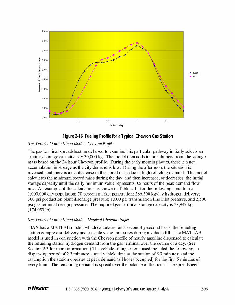
0.0%
1.0%
2.0%
3.0%
4.0%
5.0%
6.0%
7.0%
8.0%
9.0%
0 5 10 15 20
24 hour day
Perc
ent o
f Day
's T
rans
actio
ns
MonFri
Figure 2-16 Fueling Profile for a Typical Chevron Gas Station Gas Terminal Spreadsheet Model - Chevron Profile The gas terminal spreadsheet model used to examine this particular pathway initially selects an arbitrary storage capacity, say 30,000 kg. The model then adds to, or subtracts from, the storage mass based on the 24 hour Chevron profile. During the early morning hours, there is a net accumulation in storage as the city demand is low. During the afternoon, the situation is reversed, and there is a net decrease in the stored mass due to high refueling demand. The model calculates the minimum stored mass during the day, and then increases, or decreases, the initial storage capacity until the daily minimum value represents 0.5 hours of the peak demand flow rate. An example of the calculations is shown in Table 2-14 for the following conditions: 1,000,000 city population; 70 percent market penetration; 286,500 kg/day hydrogen delivery; 300 psi production plant discharge pressure; 1,000 psi transmission line inlet pressure, and 2,500 psi gas terminal design pressure. The required gas terminal storage capacity is 78,949 kg (174,053 lb).
Gas Terminal Spreadsheet Model - Modified Chevron Profile TIAX has a MATLAB model, which calculates, on a second-by-second basis, the refueling station compressor delivery and cascade vessel pressures during a vehicle fill. The MATLAB model is used in conjunction with the Chevron profile of hourly gasoline dispensed to calculate the refueling station hydrogen demand from the gas terminal over the course of a day. (See Section 2.3 for more information.) The vehicle filling criteria used included the following: a dispensing period of 2.7 minutes; a total vehicle time at the station of 5.7 minutes; and the assumption the station operates at peak demand (all hoses occupied) for the first 5 minutes of every hour. The remaining demand is spread over the balance of the hour. The spreadsheet
DE-FG36-05GO15032: Hydrogen Delivery Infrastructure Options Analysis 2-36
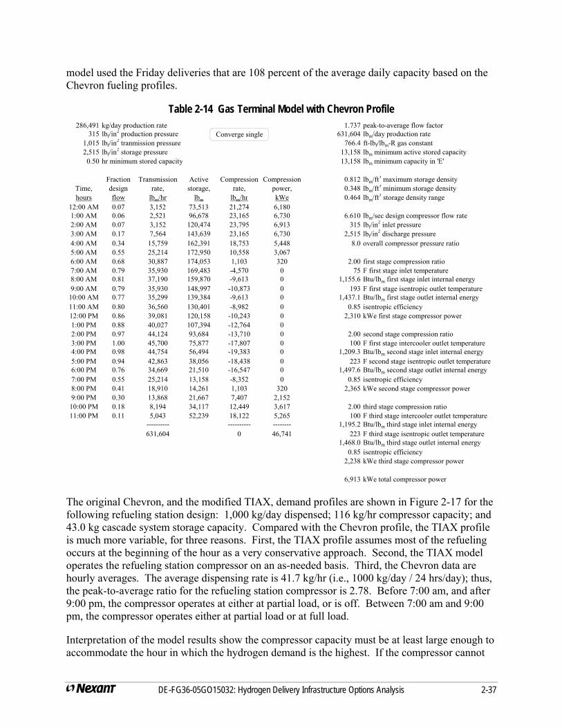
model used the Friday deliveries that are 108 percent of the average daily capacity based on the Chevron fueling profiles.
Table 2-14 Gas Terminal Model with Chevron Profile 286,491 kg/day production rate 1.737 peak-to-average flow factor
315 lbf/in2 production pressure 631,604 lbm/day production rate
1,015 lbf/in2 tranmission pressure 766.4 ft-lbf/lbm-R gas constant
2,515 lbf/in2 storage pressure 13,158 lbm minimum active stored capacity
0.50 hr minimum stored capacity 13,158 lbm minimum capacity in 'E'
Fraction Transmission Active Compression Compression 0.812 lbm/ft3 maximum storage densityTime, design rate, storage, rate, power, 0.348 lbm/ft3 minimum storage densityhours flow lbm/hr lbm lbm/hr kWe 0.464 lbm/ft3 storage density range
12:00 AM 0.07 3,152 73,513 21,274 6,1801:00 AM 0.06 2,521 96,678 23,165 6,730 6.610 lbm/sec design compressor flow rate2:00 AM 0.07 3,152 120,474 23,795 6,913 315 lbf/in
2 inlet pressure3:00 AM 0.17 7,564 143,639 23,165 6,730 2,515 lbf/in
2 discharge pressure4:00 AM 0.34 15,759 162,391 18,753 5,448 8.0 overall compressor pressure ratio5:00 AM 0.55 25,214 172,950 10,558 3,0676:00 AM 0.68 30,887 174,053 1,103 320 2.00 first stage compression ratio7:00 AM 0.79 35,930 169,483 -4,570 0 75 F first stage inlet temperature8:00 AM 0.81 37,190 159,870 -9,613 0 1,155.6 Btu/lbm first stage inlet internal energy9:00 AM 0.79 35,930 148,997 -10,873 0 193 F first stage isentropic outlet temperature
10:00 AM 0.77 35,299 139,384 -9,613 0 1,437.1 Btu/lbm first stage outlet internal energy11:00 AM 0.80 36,560 130,401 -8,982 0 0.85 isentropic efficiency12:00 PM 0.86 39,081 120,158 -10,243 0 2,310 kWe first stage compressor power1:00 PM 0.88 40,027 107,394 -12,764 02:00 PM 0.97 44,124 93,684 -13,710 0 2.00 second stage compression ratio3:00 PM 1.00 45,700 75,877 -17,807 0 100 F first stage intercooler outlet temperature4:00 PM 0.98 44,754 56,494 -19,383 0 1,209.3 Btu/lbm second stage inlet internal energy5:00 PM 0.94 42,863 38,056 -18,438 0 223 F second stage isentropic outlet temperature6:00 PM 0.76 34,669 21,510 -16,547 0 1,497.6 Btu/lbm second stage outlet internal energy7:00 PM 0.55 25,214 13,158 -8,352 0 0.85 isentropic efficiency8:00 PM 0.41 18,910 14,261 1,103 320 2,365 kWe second stage compressor power9:00 PM 0.30 13,868 21,667 7,407 2,15210:00 PM 0.18 8,194 34,117 12,449 3,617 2.00 third stage compression ratio11:00 PM 0.11 5,043 52,239 18,122 5,265 100 F third stage intercooler outlet temperature
---------- ---------- -------- 1,195.2 Btu/lbm third stage inlet internal energy631,604 0 46,741 223 F third stage isentropic outlet temperature
1,468.0 Btu/lbm third stage outlet internal energy0.85 isentropic efficiency
2,238 kWe third stage compressor power
6,913 kWe total compressor power
Converge single
The original Chevron, and the modified TIAX, demand profiles are shown in Figure 2-17 for the following refueling station design: 1,000 kg/day dispensed; 116 kg/hr compressor capacity; and 43.0 kg cascade system storage capacity. Compared with the Chevron profile, the TIAX profile is much more variable, for three reasons. First, the TIAX profile assumes most of the refueling occurs at the beginning of the hour as a very conservative approach. Second, the TIAX model operates the refueling station compressor on an as-needed basis. Third, the Chevron data are hourly averages. The average dispensing rate is 41.7 kg/hr (i.e., 1000 kg/day / 24 hrs/day); thus, the peak-to-average ratio for the refueling station compressor is 2.78. Before 7:00 am, and after 9:00 pm, the compressor operates at either at partial load, or is off. Between 7:00 am and 9:00 pm, the compressor operates either at partial load or at full load.
Interpretation of the model results show the compressor capacity must be at least large enough to accommodate the hour in which the hydrogen demand is the highest. If the compressor cannot
DE-FG36-05GO15032: Hydrogen Delivery Infrastructure Options Analysis 2-37

meet this demand, the capacity and cost of the cascade storage system increase rapidly. (See Section 2.3.)
-0 .1
0 .0
0 .1
0 .2
0 .3
0 .4
0 .5
0 .6
0 .7
0 .8
0 .9
1 .0
1 .1
1 2 :0 0A M
2 :0 0A M
4 :0 0A M
6 :0 0A M
8 :0 0A M
1 0 :0 0A M
1 2 :0 0P M
2 :0 0P M
4 :0 0P M
6 :0 0P M
8 :0 0P M
1 0 :0 0P M
1 2 :0 0A M
T im e
Frac
tion
of p
eak
deliv
ery
C h ev ro n T IA X
Figure 2-17 Chevron and Modified TIAX Refueling Station Demand Profile (Refueling Station Compressor Peak-to-Average Flow Ratio of 2.8)
The TIAX profile is a result of the relative capacities of the refueling station compressor and the cascade charging system. This profile, in essence, becomes the demand profile for the gas terminal, and the terminal capacity must be selected to satisfy this demand.
The gas terminal spreadsheet model was modified slightly to accept the TIAX profile, as shown in Table 2-15; only the first 12 hours of the day are shown. For a city demand of 286,500 kg/day, and a refueling station peak-to-average flow demand ratio of 1.5, the required gas terminal storage capacity is 85,434 kg (187,992 lb). Even though the TIAX profile is highly variable, the effect on the terminal capacity is moderate.
The costs associated with an 85,434 kg gas terminal storage capacity, a refueling station compressor capacity of 63 kg/hr, and a cascade charging system capacity of 117.6 kg represent one combination for the delivery infrastructure. To determine the combination which offers the lowest infrastructure cost, TIAX developed demand profiles for the combinations of refueling station compressor and cascade charging system capacities shown in Table 2-16. The associated gas terminal capacities to satisfy the profiles are also shown in the table. In all cases, the required gas terminal compressor power rating is 7,640 kWe.
DE-FG36-05GO15032: Hydrogen Delivery Infrastructure Options Analysis 2-38
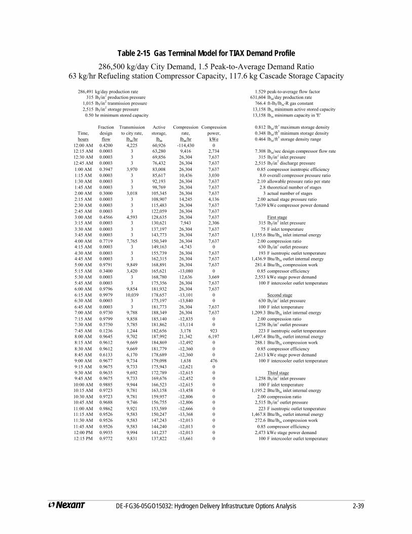
Table 2-15 Gas Terminal Model for TIAX Demand Profile 286,500 kg/day City Demand, 1.5 Peak-to-Average Demand Ratio
63 kg/hr Refueling station Compressor Capacity, 117.6 kg Cascade Storage Capacity
286,491 kg/day production rate 1.529 peak-to-average flow factor315 lbf/in
2 production pressure 631,604 lbm/day production rate1,015 lbf/in
2 tranmission pressure 766.4 ft-lbf/lbm-R gas constant2,515 lbf/in
2 storage pressure 13,158 lbm minimum active stored capacity0.50 hr minimum stored capacity 13,158 lbm minimum capacity in 'E'
Fraction Transmission Active Compression Compression 0.812 lbm/ft3 maximum storage densityTime, design to city rate, storage, rate, power, 0.348 lbm/ft3 minimum storage densityhours flow lbm/hr lbm lbm/hr kWe 0.464 lbm/ft3 storage density range
12:00 AM 0.4200 4,225 60,926 -114,430 012:15 AM 0.0003 3 63,280 9,416 2,734 7.308 lbm/sec design compressor flow rate12:30 AM 0.0003 3 69,856 26,304 7,637 315 lbf/in
2 inlet pressure12:45 AM 0.0003 3 76,432 26,304 7,637 2,515 lbf/in
2 discharge pressure1:00 AM 0.3947 3,970 83,008 26,304 7,637 0.85 compressor isentropic efficiency1:15 AM 0.0003 3 85,617 10,436 3,030 8.0 overall compressor pressure ratio1:30 AM 0.0003 3 92,193 26,304 7,637 2.10 allowable pressure ratio per state1:45 AM 0.0003 3 98,769 26,304 7,637 2.8 theoretical number of stages2:00 AM 0.3000 3,018 105,345 26,304 7,637 3 actual number of stages2:15 AM 0.0003 3 108,907 14,245 4,136 2.00 actual stage pressure ratio2:30 AM 0.0003 3 115,483 26,304 7,637 7,639 kWe compressor power demand2:45 AM 0.0003 3 122,059 26,304 7,6373:00 AM 0.4566 4,593 128,635 26,304 7,637 First stage3:15 AM 0.0003 3 130,621 7,943 2,306 315 lbf/in
2 inlet pressure3:30 AM 0.0003 3 137,197 26,304 7,637 75 F inlet temperature3:45 AM 0.0003 3 143,773 26,304 7,637 1,155.6 Btu/lbm inlet internal energy4:00 AM 0.7719 7,765 150,349 26,304 7,637 2.00 compression ratio4:15 AM 0.0003 3 149,163 -4,743 0 630 lbf/in
2 outlet pressure4:30 AM 0.0003 3 155,739 26,304 7,637 193 F isentropic outlet temperature4:45 AM 0.0003 3 162,315 26,304 7,637 1,436.9 Btu/lbm outlet internal energy5:00 AM 0.9791 9,849 168,891 26,304 7,637 281.4 Btu/lbm compression work5:15 AM 0.3400 3,420 165,621 -13,080 0 0.85 compressor efficiency5:30 AM 0.0003 3 168,780 12,636 3,669 2,553 kWe stage power demand5:45 AM 0.0003 3 175,356 26,304 7,637 100 F intercooler outlet temperature6:00 AM 0.9796 9,854 181,932 26,304 7,6376:15 AM 0.9979 10,039 178,657 -13,101 0 Second stage6:30 AM 0.0003 3 175,197 -13,840 0 630 lbf/in
2 inlet pressure6:45 AM 0.0003 3 181,773 26,304 7,637 100 F inlet temperature7:00 AM 0.9730 9,788 188,349 26,304 7,637 1,209.3 Btu/lbm inlet internal energy7:15 AM 0.9799 9,858 185,140 -12,835 0 2.00 compression ratio7:30 AM 0.5750 5,785 181,862 -13,114 0 1,258 lbf/in
2 outlet pressure7:45 AM 0.1236 1,244 182,656 3,178 923 223 F isentropic outlet temperature8:00 AM 0.9645 9,702 187,992 21,342 6,197 1,497.4 Btu/lbm outlet internal energy8:15 AM 0.9612 9,669 184,869 -12,492 0 288.1 Btu/lbm compression work8:30 AM 0.9612 9,669 181,779 -12,360 0 0.85 compressor efficiency8:45 AM 0.6133 6,170 178,689 -12,360 0 2,613 kWe stage power demand9:00 AM 0.9677 9,734 179,098 1,638 476 100 F intercooler outlet temperature9:15 AM 0.9675 9,733 175,943 -12,621 09:30 AM 0.9635 9,692 172,789 -12,615 0 Third stage9:45 AM 0.9675 9,733 169,676 -12,452 0 1,258 lbf/in
2 inlet pressure10:00 AM 0.9885 9,944 166,523 -12,615 0 100 F inlet temperature10:15 AM 0.9723 9,781 163,158 -13,458 0 1,195.2 Btu/lbm inlet internal energy10:30 AM 0.9723 9,781 159,957 -12,806 0 2.00 compression ratio10:45 AM 0.9688 9,746 156,755 -12,806 0 2,515 lbf/in
2 outlet pressure11:00 AM 0.9862 9,921 153,589 -12,666 0 223 F isentropic outlet temperature11:15 AM 0.9526 9,583 150,247 -13,368 0 1,467.8 Btu/lbm outlet internal energy11:30 AM 0.9526 9,583 147,243 -12,013 0 272.6 Btu/lbm compression work11:45 AM 0.9526 9,583 144,240 -12,013 0 0.85 compressor efficiency12:00 PM 0.9935 9,994 141,237 -12,013 0 2,473 kWe stage power demand12:15 PM 0.9772 9,831 137,822 -13,661 0 100 F intercooler outlet temperature
DE-FG36-05GO15032: Hydrogen Delivery Infrastructure Options Analysis 2-39
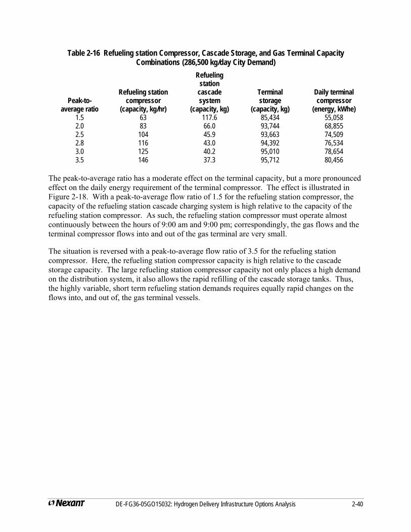
Table 2-16 Refueling station Compressor, Cascade Storage, and Gas Terminal Capacity Combinations (286,500 kg/day City Demand)
Peak-to-average ratio
Refueling station compressor
(capacity, kg/hr)
Refueling station
cascade system
(capacity, kg)
Terminal storage
(capacity, kg)
Daily terminal compressor
(energy, kWhe) 1.5 63 117.6 85,434 55,058 2.0 83 66.0 93,744 68,855 2.5 104 45.9 93,663 74,509 2.8 116 43.0 94,392 76,534 3.0 125 40.2 95,010 78,654 3.5 146 37.3 95,712 80,456
The peak-to-average ratio has a moderate effect on the terminal capacity, but a more pronounced effect on the daily energy requirement of the terminal compressor. The effect is illustrated in Figure 2-18. With a peak-to-average flow ratio of 1.5 for the refueling station compressor, the capacity of the refueling station cascade charging system is high relative to the capacity of the refueling station compressor. As such, the refueling station compressor must operate almost continuously between the hours of 9:00 am and 9:00 pm; correspondingly, the gas flows and the terminal compressor flows into and out of the gas terminal are very small.
The situation is reversed with a peak-to-average flow ratio of 3.5 for the refueling station compressor. Here, the refueling station compressor capacity is high relative to the cascade storage capacity. The large refueling station compressor capacity not only places a high demand on the distribution system, it also allows the rapid refilling of the cascade storage tanks. Thus, the highly variable, short term refueling station demands requires equally rapid changes on the flows into, and out of, the gas terminal vessels.
DE-FG36-05GO15032: Hydrogen Delivery Infrastructure Options Analysis 2-40
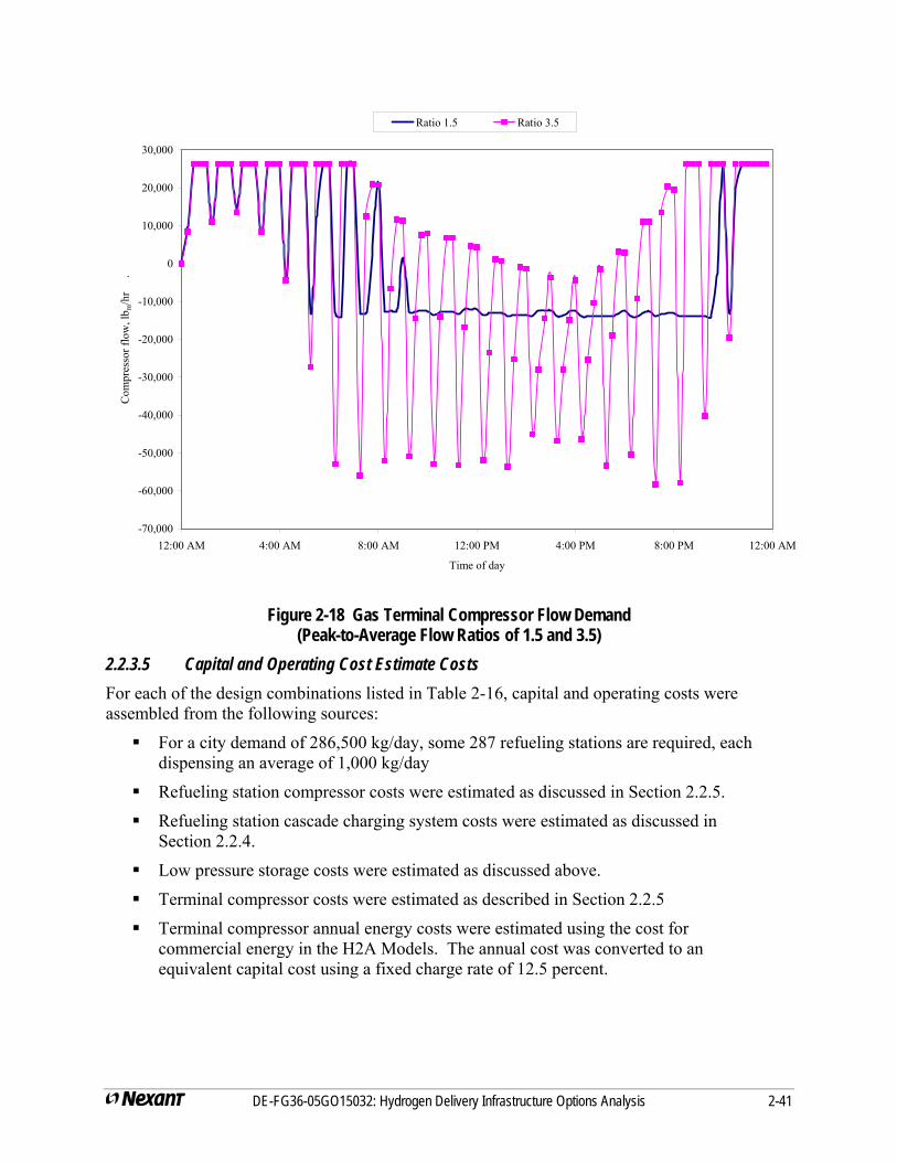
-70,000
-60,000
-50,000
-40,000
-30,000
-20,000
-10,000
0
10,000
20,000
30,000
12:00 AM 4:00 AM 8:00 AM 12:00 PM 4:00 PM 8:00 PM 12:00 AM
Time of day
Com
pres
sor f
low
, lb m
/hr
.
Ratio 1.5 Ratio 3.5
Figure 2-18 Gas Terminal Compressor Flow Demand (Peak-to-Average Flow Ratios of 1.5 and 3.5)
2.2.3.5 Capital and Operating Cost Estimate Costs For each of the design combinations listed in Table 2-16, capital and operating costs were assembled from the following sources:
For a city demand of 286,500 kg/day, some 287 refueling stations are required, each dispensing an average of 1,000 kg/day
Refueling station compressor costs were estimated as discussed in Section 2.2.5.
Refueling station cascade charging system costs were estimated as discussed in Section 2.2.4.
Low pressure storage costs were estimated as discussed above.
Terminal compressor costs were estimated as described in Section 2.2.5
Terminal compressor annual energy costs were estimated using the cost for commercial energy in the H2A Models. The annual cost was converted to an equivalent capital cost using a fixed charge rate of 12.5 percent.
DE-FG36-05GO15032: Hydrogen Delivery Infrastructure Options Analysis 2-41

The results of the cost calculations are shown in Figure 2-19. The lowest infrastructure costs occur with the smallest peak-to-average ratios for the refueling station compressor. However, the total infrastructure costs show only a small variation over the range of 1.5 to 2.5.
$265,000
$270,000
$275,000
$280,000
$285,000
$290,000
$295,000
1.5 2.0 2.5 3.0 3.5
Peak-to-average flow ratio
Term
ianl
+ fo
reco
urt c
osts,
$10
00
Figure 2-19 Gas Terminal and Refueling Station Cost Estimates (286,500 kg/day City Demand)
2.2.3.6 Recommended Inputs to the H2A Model For the purposes of the study, the following approach was used in the development of the low pressure storage costs and capacities:
System reliability and availability should be improved by selecting the fewest number of vessels as possible. The availability of the vessels will be essentially 100 percent. However, the associated isolation and pressure relief valves are likely to be more problematic, and the highest availability should result from the fewest components. As a result, larger vessels should be preferred.
The largest vessels analyzed above are those based on the use of SA516 Grade 70 carbon steel; i.e., 2.5 inch wall thickness, 4.1 feet in diameter, 24.9 feet long, and storing 91 kilograms of hydrogen. The approximate weight of each vessel is 32,200 pounds.
The unit cost to fabricate a vessel using SA516 carbon steel is $1.91 per pound of steel, as estimated by the Icarus program. The unit fabrication cost for a chromium-molybdenum steel vessel from CP Industries is approximately $2.62 per pound of steel. For the purposes of this study, a unit fabrication cost equal to the average of the above costs, or $2.30 per pound of steel, has been assumed. Although the gas terminal vessels will be fabricated from carbon steel, there will likely need to be
DE-FG36-05GO15032: Hydrogen Delivery Infrastructure Options Analysis 2-42
fairly strict controls on the steel chemistry, together with limits on the maximum grain size, to provide the desired resistance to hydrogen embrittlement in cyclic pressure service. The estimated FOB price for the fabricated vessel is then $74,000, or $816 per kilogram of hydrogen.
With a vessel weight of 16 tons, a commercial truck is limited to transporting 2 vessels. Assuming a shipping distance of 1,500 miles from the fabrication plant to the gas terminal, and a unit truck expense of $2.50 per mile, the delivered price of the vessel is $75,900, or $837 per kilogram of hydrogen.
Assuming a sales tax rate of 7.5 percent, the total delivered (uninstalled) price for a vessel would be $81,600, or $900 per kilogram of hydrogen.
Based on the analysis in Section 2.2.4 for the cost of installing gaseous hydrogen storage vessels, an installation factor of 1.3 is recommended and used for these low pressure gaseous hydrogen storage vessels in the H2A Delivery Models Version 2.
Although the analysis above was done specifically for gas storage located at a terminal, the primary conclusions and approach are applicable and are used for gas storage located at the refueling site on the H2A Delivery Models Version 2. (See Section 2.1.9 that explains the advantages to gas storage at the refueling site compared to at a terminal in a hydrogen pipeline delivery infrastructure to handle the hourly refueling site demand profile.)
2.2.4 Cascade Charging System Vessels Hydrogen refueling station designs will likely use a combination of compressor capacity and cascade storage system capacity for filling fuel cell vehicles. The sections below describe the development of a unit capital cost for refueling station cascade vessels, in $ per kilogram of hydrogen, for use in the H2A Delivery Component and HDSAM Models.
2.2.4.1 Pressure Vessel Fabrication Costs The basic refueling station storage module is assumed to consist of 3 pressure vessels, a support structure, and associated valves and plumbing. A potential module arrangement is shown in Figure 2-20. Although the vessels shown in the figure are composite vessels under development, steel vessel arrangements look very similar. The peak pressure of these vessels can be 6,250 psi but each may have different minimum pressures. (See Section 2.1.5).
DE-FG36-05GO15032: Hydrogen Delivery Infrastructure Options Analysis 2-43
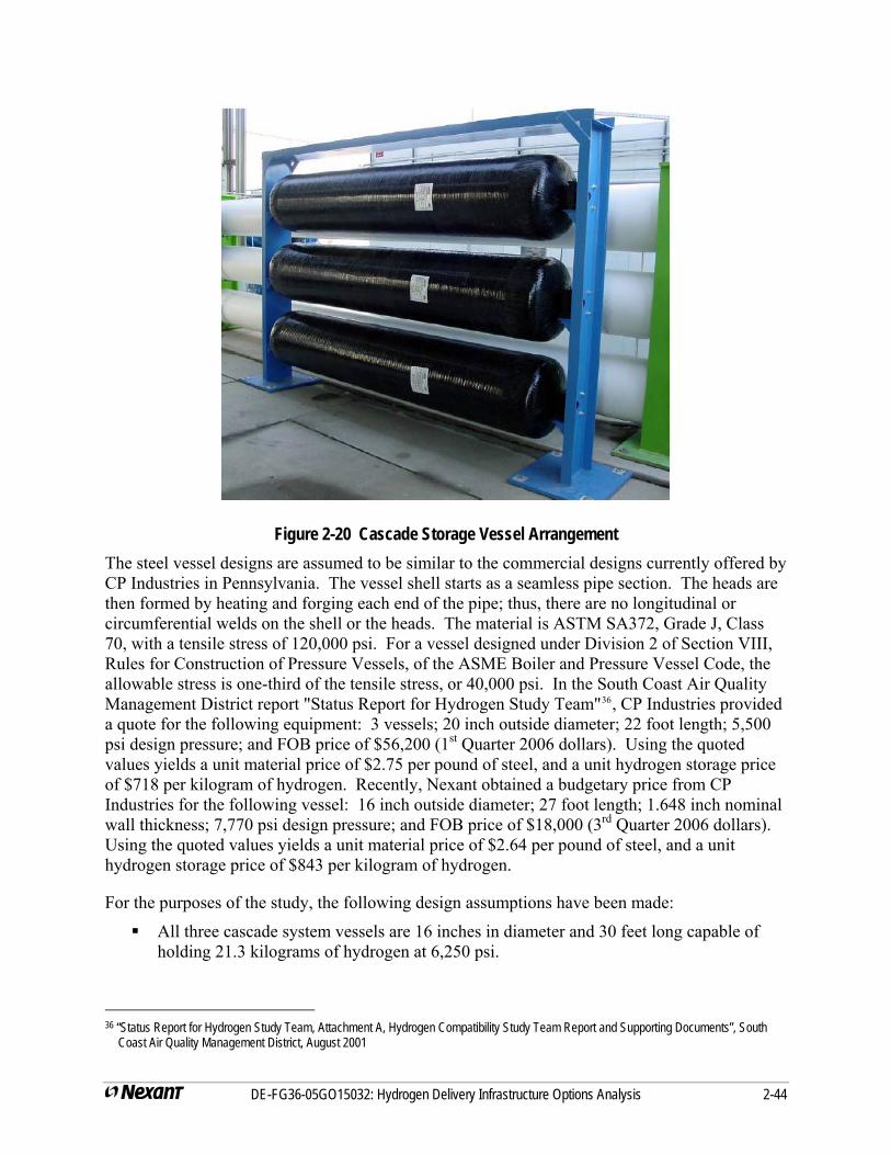
DE-FG36-05GO15032: Hydrogen Delivery Infrastructure Options Analysis 2-44
Figure 2-20 Cascade Storage Vessel Arrangement The steel vessel designs are assumed to be similar to the commercial designs currently offered by CP Industries in Pennsylvania. The vessel shell starts as a seamless pipe section. The heads are then formed by heating and forging each end of the pipe; thus, there are no longitudinal or circumferential welds on the shell or the heads. The material is ASTM SA372, Grade J, Class 70, with a tensile stress of 120,000 psi. For a vessel designed under Division 2 of Section VIII, Rules for Construction of Pressure Vessels, of the ASME Boiler and Pressure Vessel Code, the allowable stress is one-third of the tensile stress, or 40,000 psi. In the South Coast Air Quality Management District report "Status Report for Hydrogen Study Team"36, CP Industries provided a quote for the following equipment: 3 vessels; 20 inch outside diameter; 22 foot length; 5,500 psi design pressure; and FOB price of $56,200 (1st Quarter 2006 dollars). Using the quoted values yields a unit material price of $2.75 per pound of steel, and a unit hydrogen storage price of $718 per kilogram of hydrogen. Recently, Nexant obtained a budgetary price from CP Industries for the following vessel: 16 inch outside diameter; 27 foot length; 1.648 inch nominal wall thickness; 7,770 psi design pressure; and FOB price of $18,000 (3rd Quarter 2006 dollars). Using the quoted values yields a unit material price of $2.64 per pound of steel, and a unit hydrogen storage price of $843 per kilogram of hydrogen.
For the purposes of the study, the following design assumptions have been made:
All three cascade system vessels are 16 inches in diameter and 30 feet long capable of holding 21.3 kilograms of hydrogen at 6,250 psi.
36 “Status Report for Hydrogen Study Team, Attachment A, Hydrogen Compatibility Study Team Report and Supporting Documents”, South
Coast Air Quality Management District, August 2001
A unit storage price of $843 per kilogram of hydrogen applied to the high, the intermediate, and the low pressure vessels. With an assumed sales tax rate of 7.5 percent, the purchased vessel price is $906 per kilogram of hydrogen.
The bare vessels are shipped an average distance of 1,500 miles to an assembly facility, where the 3 vessels are mounted in the support frame. Nine bare vessels, with a combined weight of 50,000 pounds, can be shipped on a flat bed truck. Assuming a shipping cost of $2.50 per mile, the delivered (uninstalled) vessel price is then $926 per kilogram of hydrogen.
2.2.4.2 Pressure Vessel Auxiliaries and Installation Costs At the assembly facility, the 3 vessels are mounted in a support frame, and the requisite valves and plumbing are added. The 3-vessel assemblies are then shipped 250 miles to a refueling station, lifted from the truck with a crane, and bolted to a set of concrete anchor bolts. Plumbing connections between the vessel assemblies and the dispensers completes the storage installation. The estimated cost for the vessel supports, valves, plumbing, leak tests, shipping, and installation is $18,102 as shown in Table 2-17.
The shop fabrication labor rate of $85/hr and the field installation rate of $65/hr are recommended values from the Bechtel cost engineering group. The rates include all overhead expenses, together with various miscellaneous expenses, such as preparation of shop drawings and the documentation of ASME tests.
Prices for the auxiliary equipment, such as valves, tubing, and fittings, were obtained from the McMaster-Carr web site. One might argue that purchasing the items directly from the equipment suppliers would result in lower prices. However, McMaster-Carr has a substantial sales volume, and the premium for ordering through McMaster-Carr is likely well within the accuracy of the estimate.
A commercial source for compression fittings, valves, and high pressure tubing is Swagelok. A review of the Swagelok equipment catalog shows pressure rating of 6,000 psi for tubing and valves to be reasonably common for tubing diameters up, and including, ½ inch. Moving to ¾ inch fittings and valves typically results in a pressure rating of only 5,000 psi. Thus, for the purposes of the cost study, a tube and valve size of ½ inch has been assumed. A quick check on the flow coefficients for ½ inch ball valves shows the pressure losses to be very modest.
Flows to and from the vessels are modulated by the 'vessel pressure maintenance valves', and as such, a programmable logic controller will not be required at the refueling station to control the operation of the compressor or the charging/discharging of the storage vessels.
The operation of the compressor is assumed to be controlled by a pressure switch on the high pressure cylinder. For pressures below 6,000 psi, the switch energizes a relay, which closes a contactor supplying electric power to the motor. When the pressure reaches 6,250 psi, the switch opens, and the compressor stops.
All Valves are manual; there are no pneumatically or electrically operated valves.
The 3-vessel combination stores a total of 65 kilogram of hydrogen, yielding a unit cost of $278 per kilogram for the vessel supports and auxiliaries.
DE-FG36-05GO15032: Hydrogen Delivery Infrastructure Options Analysis 2-45
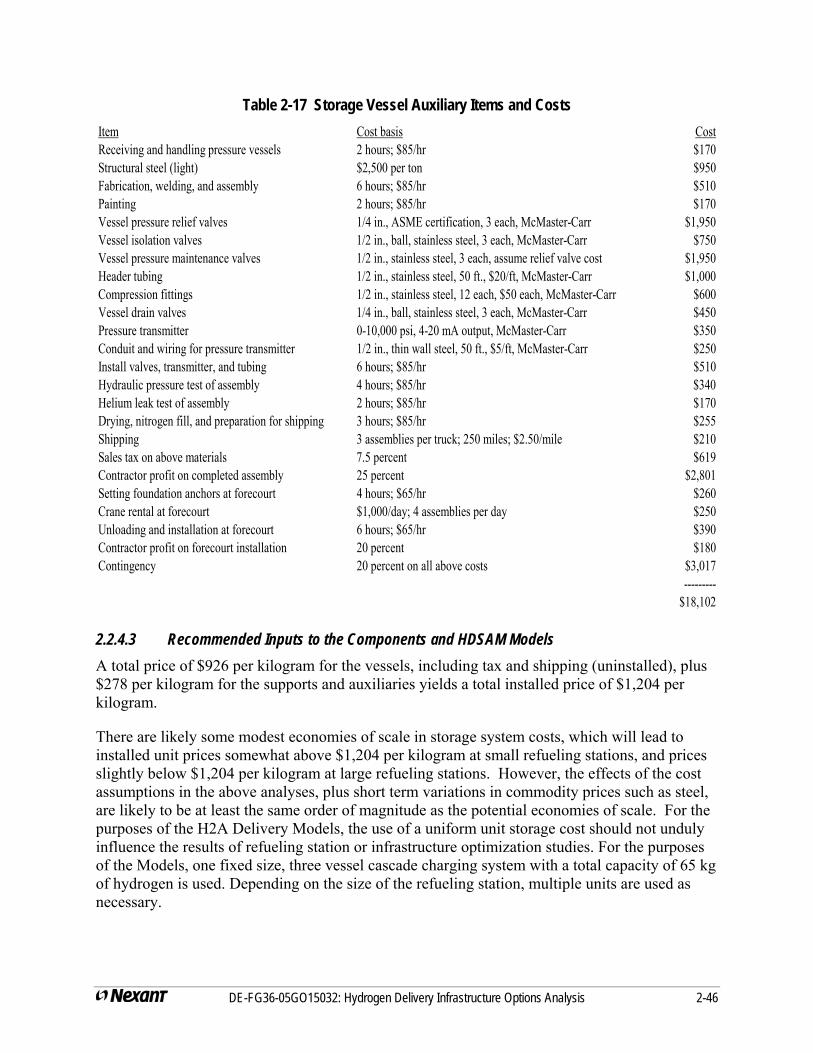
Table 2-17 Storage Vessel Auxiliary Items and Costs Item Cost basis CostReceiving and handling pressure vessels 2 hours; $85/hr $170Structural steel (light) $2,500 per ton $950Fabrication, welding, and assembly 6 hours; $85/hr $510Painting 2 hours; $85/hr $170Vessel pressure relief valves 1/4 in., ASME certification, 3 each, McMaster-Carr $1,950Vessel isolation valves 1/2 in., ball, stainless steel, 3 each, McMaster-Carr $750Vessel pressure maintenance valves 1/2 in., stainless steel, 3 each, assume relief valve cost $1,950Header tubing 1/2 in., stainless steel, 50 ft., $20/ft, McMaster-Carr $1,000Compression fittings 1/2 in., stainless steel, 12 each, $50 each, McMaster-Carr $600Vessel drain valves 1/4 in., ball, stainless steel, 3 each, McMaster-Carr $450Pressure transmitter 0-10,000 psi, 4-20 mA output, McMaster-Carr $350Conduit and wiring for pressure transmitter 1/2 in., thin wall steel, 50 ft., $5/ft, McMaster-Carr $250Install valves, transmitter, and tubing 6 hours; $85/hr $510Hydraulic pressure test of assembly 4 hours; $85/hr $340Helium leak test of assembly 2 hours; $85/hr $170Drying, nitrogen fill, and preparation for shipping 3 hours; $85/hr $255Shipping 3 assemblies per truck; 250 miles; $2.50/mile $210Sales tax on above materials 7.5 percent $619Contractor profit on completed assembly 25 percent $2,801Setting foundation anchors at forecourt 4 hours; $65/hr $260Crane rental at forecourt $1,000/day; 4 assemblies per day $250Unloading and installation at forecourt 6 hours; $65/hr $390Contractor profit on forecourt installation 20 percent $180Contingency 20 percent on all above costs $3,017
---------$18,102
2.2.4.3 Recommended Inputs to the Components and HDSAM Models A total price of $926 per kilogram for the vessels, including tax and shipping (uninstalled), plus $278 per kilogram for the supports and auxiliaries yields a total installed price of $1,204 per kilogram.
There are likely some modest economies of scale in storage system costs, which will lead to installed unit prices somewhat above $1,204 per kilogram at small refueling stations, and prices slightly below $1,204 per kilogram at large refueling stations. However, the effects of the cost assumptions in the above analyses, plus short term variations in commodity prices such as steel, are likely to be at least the same order of magnitude as the potential economies of scale. For the purposes of the H2A Delivery Models, the use of a uniform unit storage cost should not unduly influence the results of refueling station or infrastructure optimization studies. For the purposes of the Models, one fixed size, three vessel cascade charging system with a total capacity of 65 kg of hydrogen is used. Depending on the size of the refueling station, multiple units are used as necessary.
DE-FG36-05GO15032: Hydrogen Delivery Infrastructure Options Analysis 2-46
2.2.5 Transmission, Terminal, and Refueling Station Compressors 2.2.5.1 Transmission and Terminal Compressors For medium to large cities, with significant market penetrations for fuel cell vehicles, compressors with power ratings from 1 to several MWe will be required for pipeline delivery pathways and gaseous hydrogen terminal and tube trailer operations. This report outlines recommended approaches for estimating the power requirements and the installed capital costs for large compressors.
Current technology for large hydrogen compressors suitable for transmission line compressors are reciprocating compressors, as opposed to centrifugal machines used for natural gas. A centrifugal compressor increases the pressure in a gas by accelerating the gas in the rotating section, and then converting the kinetic energy to static pressure in the stationary section. Since the kinetic energy is proportional to density x velocity2, the change in pressure is proportional to the gas density. Further, the density varies linearly with the molecular weight, and there are strong Mach number limits on allowable gas velocities within the compressor. As a result, for a given pressure ratio, the number of stages for a hydrogen centrifugal compressor will be 8 times the number of stages for existing natural gas compressor technology, and 14 times the number of stages for an air compressor. Since the cost of a compressor is, to a first order, proportional to the number of stages, the cost for a centrifugal unit would be impractically high for the pressure ratios required in a transmission line compressor. New concepts for hydrogen centrifugal compressors that could be very cost effective are being researched. Reciprocating compressors are used in the H2A Delivery Models for large hydrogen compression flows to represent currently available technology.
For the purposes of the analysis, the suction pressure for the transmission line compressor is assumed to be 300 psi from the central hydrogen production plant. The maximum allowable gas temperature during compression is taken to be 275°F, based on the requirements of American Petroleum Institute Standard 618, Reciprocating Compressors for Petroleum, Chemical, and Gas Industry Service. For the thermodynamic properties of hydrogen, and with the isentropic efficiencies described below, the allowable pressure ratio per stage of compression used is 2.1.
Reciprocating Compressor Types With transmission line pressures in the range of 1,000 psi, gas storage in the range of 2,500 psi at tube trailer terminals, and compressor inlet pressures in the range of 300 to 1,000 psi, the overall pressure ratio for the large compressors will be in the range of 3 to 7. Assuming an allowable pressure ratio of 2.1 per stage, the compressors will require 2 to 4 stages.
Reciprocating compressors fall into two broad categories: lubricated; and non-lubricated. In a lubricated design, the iron pistons and rings are lubricated by a thin film of oil, which adheres to the cylinder walls. As such, a small quantity of oil is normally carried with the gas as it leaves the cylinder.
In a non-lubricated design, the pistons and rings are a plastic, such as Teflon, and no oil lubrication is required.
DE-FG36-05GO15032: Hydrogen Delivery Infrastructure Options Analysis 2-47
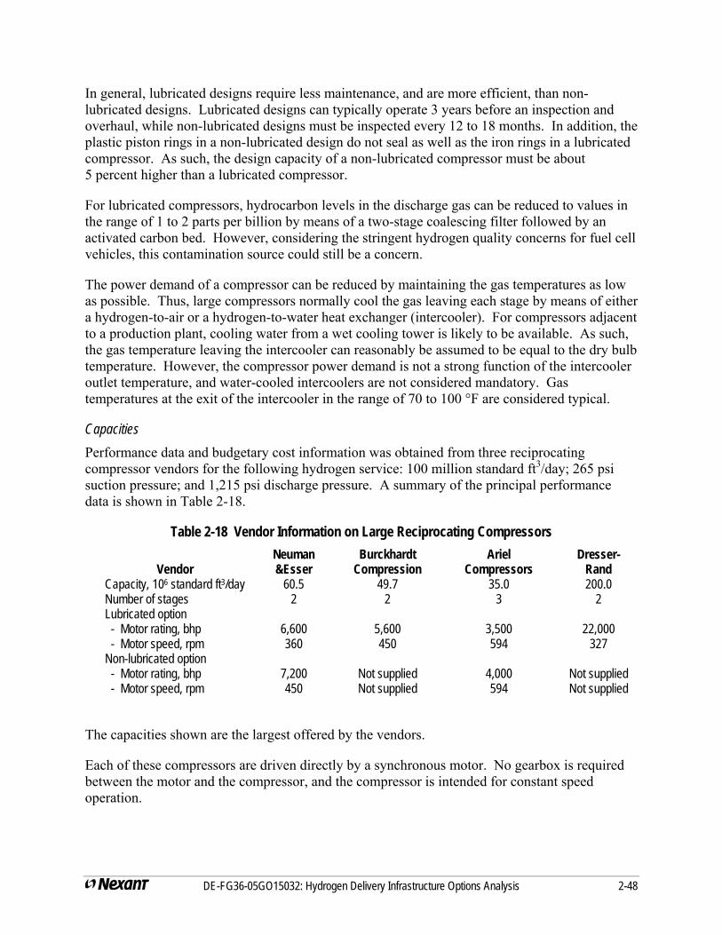
In general, lubricated designs require less maintenance, and are more efficient, than non-lubricated designs. Lubricated designs can typically operate 3 years before an inspection and overhaul, while non-lubricated designs must be inspected every 12 to 18 months. In addition, the plastic piston rings in a non-lubricated design do not seal as well as the iron rings in a lubricated compressor. As such, the design capacity of a non-lubricated compressor must be about 5 percent higher than a lubricated compressor.
For lubricated compressors, hydrocarbon levels in the discharge gas can be reduced to values in the range of 1 to 2 parts per billion by means of a two-stage coalescing filter followed by an activated carbon bed. However, considering the stringent hydrogen quality concerns for fuel cell vehicles, this contamination source could still be a concern.
The power demand of a compressor can be reduced by maintaining the gas temperatures as low as possible. Thus, large compressors normally cool the gas leaving each stage by means of either a hydrogen-to-air or a hydrogen-to-water heat exchanger (intercooler). For compressors adjacent to a production plant, cooling water from a wet cooling tower is likely to be available. As such, the gas temperature leaving the intercooler can reasonably be assumed to be equal to the dry bulb temperature. However, the compressor power demand is not a strong function of the intercooler outlet temperature, and water-cooled intercoolers are not considered mandatory. Gas temperatures at the exit of the intercooler in the range of 70 to 100 °F are considered typical.
Capacities Performance data and budgetary cost information was obtained from three reciprocating compressor vendors for the following hydrogen service: 100 million standard ft3/day; 265 psi suction pressure; and 1,215 psi discharge pressure. A summary of the principal performance data is shown in Table 2-18.
Table 2-18 Vendor Information on Large Reciprocating Compressors
Vendor Neuman &Esser
Burckhardt Compression
Ariel Compressors
Dresser-Rand
Capacity, 106 standard ft3/day 60.5 49.7 35.0 200.0 Number of stages 2 2 3 2 Lubricated option - Motor rating, bhp 6,600 5,600 3,500 22,000 - Motor speed, rpm 360 450 594 327 Non-lubricated option - Motor rating, bhp 7,200 Not supplied 4,000 Not supplied - Motor speed, rpm 450 Not supplied 594 Not supplied
The capacities shown are the largest offered by the vendors.
Each of these compressors are driven directly by a synchronous motor. No gearbox is required between the motor and the compressor, and the compressor is intended for constant speed operation.
DE-FG36-05GO15032: Hydrogen Delivery Infrastructure Options Analysis 2-48
DE-FG36-05GO15032: Hydrogen Delivery Infrastructure Options Analysis 2-49
Power Calculations and Efficiencies The power required in each stage of the compression process can be calculated as follows:
efficiency IsentropicPower
Power isentropic=
where the isentropic power is defined by the following expression:
Power isentropic, Btu/sec = (Mass flow rate, lbm/sec)(H outlet - H inlet, Btu/lbm)
with the enthalpies evaluated at the gas inlet temperature, and at the isentropic outlet temperature for each stage, per the following equation:
k1k
inlet
outletinletoutlet P
PTT
−
⎟⎟⎠
⎞⎜⎜⎝
⎛=
where k is the ratio of specific heats. For large reciprocating compressors, isentropic efficiencies in the range of 86 to 92 percent are considered typical.
In principle, the best accuracy in the calculation of the compressor power should be reached by 1) using an expression for the enthalpy which is a function of the temperature, 2) including pressure losses into, and out of, each stage, 3) using an assumed intercooler effectiveness to estimate the gas temperature entering each stage, and 4) calculating the performance of each stage, and summing over the number of stages. An example of the approach is shown in Table 2-19. The pressure losses at each stage were derived from a quote supplied by Neuman & Esser, as noted above. The isentropic efficiency was selected manually to match the calculated power with the quoted power. The stage enthalpies were calculated using the Shomate equation from the NIST Webbook, as detailed in Table 2-20.
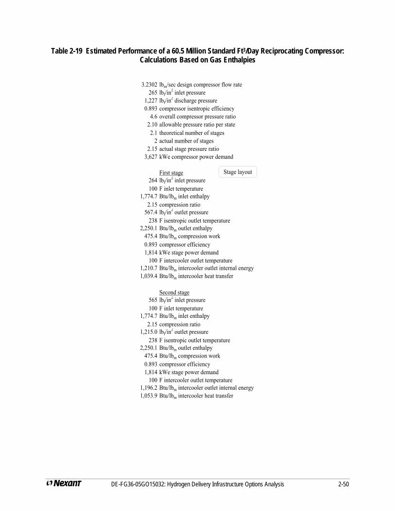
Table 2-19 Estimated Performance of a 60.5 Million Standard Ft3/Day Reciprocating Compressor: Calculations Based on Gas Enthalpies
3.2302 lbm/sec design compressor flow rate
265 lbf/in2 inlet pressure
1,227 lbf/in2 discharge pressure
0.893 compressor isentropic efficiency4.6 overall compressor pressure ratio
2.10 allowable pressure ratio per state2.1 theoretical number of stages
2 actual number of stages2.15 actual stage pressure ratio
3,627 kWe compressor power demand
First stage264 lbf/in
2 inlet pressure100 F inlet temperature
1,774.7 Btu/lbm inlet enthalpy2.15 compression ratio
567.4 lbf/in2 outlet pressure
238 F isentropic outlet temperature2,250.1 Btu/lbm outlet enthalpy
475.4 Btu/lbm compression work0.893 compressor efficiency1,814 kWe stage power demand
100 F intercooler outlet temperature1,210.7 Btu/lbm intercooler outlet internal energy1,039.4 Btu/lbm intercooler heat transfer
Second stage565 lbf/in
2 inlet pressure100 F inlet temperature
1,774.7 Btu/lbm inlet enthalpy2.15 compression ratio
1,215.0 lbf/in2 outlet pressure
238 F isentropic outlet temperature2,250.1 Btu/lbm outlet enthalpy
475.4 Btu/lbm compression work0.893 compressor efficiency1,814 kWe stage power demand
100 F intercooler outlet temperature1,196.2 Btu/lbm intercooler outlet internal energy1,053.9 Btu/lbm intercooler heat transfer
Stage layout
DE-FG36-05GO15032: Hydrogen Delivery Infrastructure Options Analysis 2-50
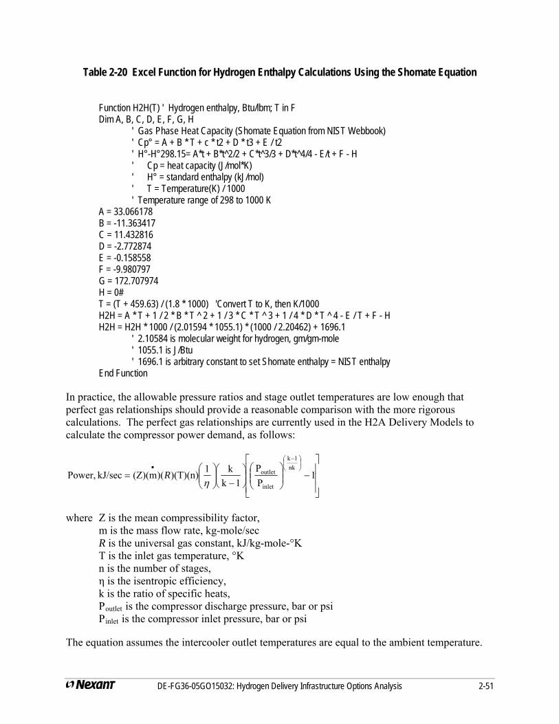
Table 2-20 Excel Function for Hydrogen Enthalpy Calculations Using the Shomate Equation
Function H2H(T) ' Hydrogen enthalpy, Btu/lbm; T in F Dim A, B, C, D, E, F, G, H ' Gas Phase Heat Capacity (Shomate Equation from NIST Webbook) ' Cp° = A + B * T + c * t2 + D * t3 + E / t2 ' H°-H°298.15= A*t + B*t^2/2 + C*t^3/3 + D*t^4/4 - E/t + F - H ' Cp = heat capacity (J/mol*K) ' H° = standard enthalpy (kJ/mol) ' T = Temperature(K) / 1000 ' Temperature range of 298 to 1000 K A = 33.066178 B = -11.363417 C = 11.432816 D = -2.772874 E = -0.158558 F = -9.980797 G = 172.707974 H = 0# T = (T + 459.63) / (1.8 * 1000) 'Convert T to K, then K/1000 H2H = A * T + 1 / 2 * B * T ^ 2 + 1 / 3 * C * T ^ 3 + 1 / 4 * D * T ^ 4 - E / T + F - H H2H = H2H * 1000 / (2.01594 * 1055.1) * (1000 / 2.20462) + 1696.1 ' 2.10584 is molecular weight for hydrogen, gm/gm-mole ' 1055.1 is J/Btu ' 1696.1 is arbitrary constant to set Shomate enthalpy = NIST enthalpy End Function In practice, the allowable pressure ratios and stage outlet temperatures are low enough that perfect gas relationships should provide a reasonable comparison with the more rigorous calculations. The perfect gas relationships are currently used in the H2A Delivery Models to calculate the compressor power demand, as follows:
⎥⎥⎥
⎦
⎤
⎢⎢⎢
⎣
⎡−⎟⎟
⎠
⎞⎜⎜⎝
⎛⎟⎠⎞
⎜⎝⎛
−⎟⎟⎠
⎞⎜⎜⎝
⎛=
⎟⎠⎞
⎜⎝⎛ −
•1
PP
1kk1)(T)(n))(m(Z)(kJ/sec Power,
nk1k
inlet
outlet
ηR
where Z is the mean compressibility factor, m is the mass flow rate, kg-mole/sec R is the universal gas constant, kJ/kg-mole-°K T is the inlet gas temperature, °K n is the number of stages, η is the isentropic efficiency, k is the ratio of specific heats, Poutlet is the compressor discharge pressure, bar or psi Pinlet is the compressor inlet pressure, bar or psi
The equation assumes the intercooler outlet temperatures are equal to the ambient temperature.
DE-FG36-05GO15032: Hydrogen Delivery Infrastructure Options Analysis 2-51
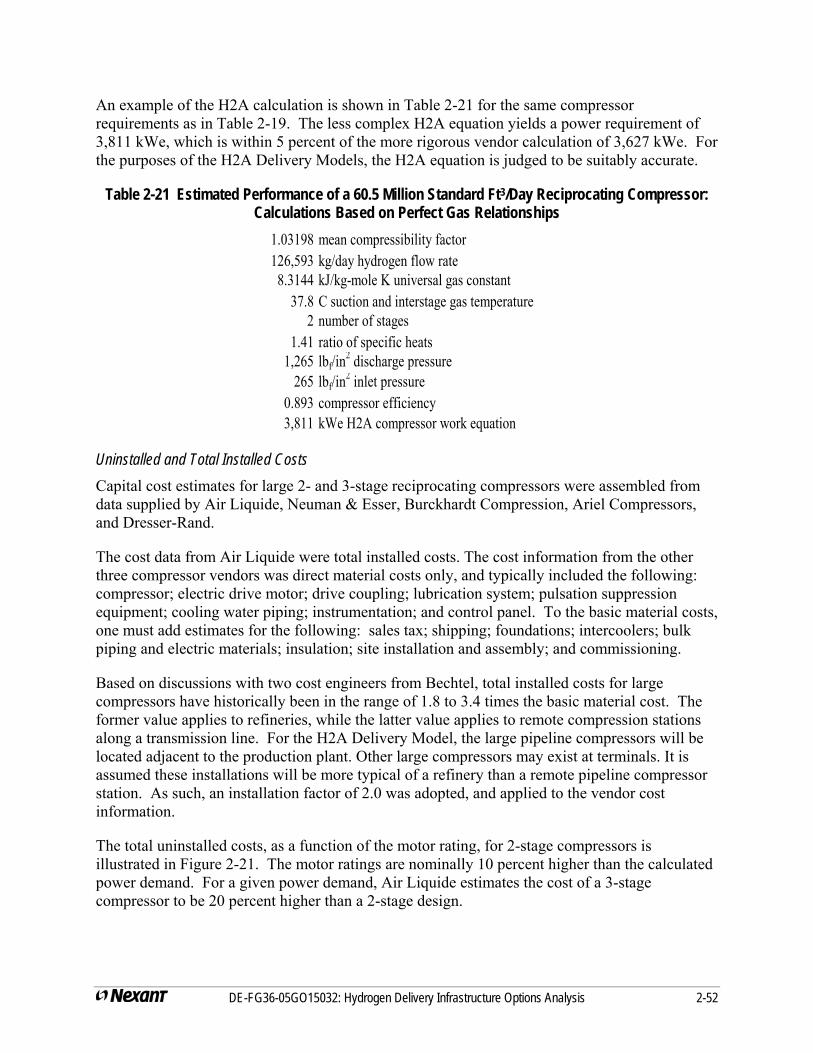
An example of the H2A calculation is shown in Table 2-21 for the same compressor requirements as in Table 2-19. The less complex H2A equation yields a power requirement of 3,811 kWe, which is within 5 percent of the more rigorous vendor calculation of 3,627 kWe. For the purposes of the H2A Delivery Models, the H2A equation is judged to be suitably accurate.
Table 2-21 Estimated Performance of a 60.5 Million Standard Ft3/Day Reciprocating Compressor: Calculations Based on Perfect Gas Relationships
1.03198 mean compressibility factor126,593 kg/day hydrogen flow rate
8.3144 kJ/kg-mole K universal gas constant37.8 C suction and interstage gas temperature
2 number of stages1.41 ratio of specific heats
1,265 lbf/in2 discharge pressure
265 lbf/in2 inlet pressure
0.893 compressor efficiency3,811 kWe H2A compressor work equation
Uninstalled and Total Installed Costs Capital cost estimates for large 2- and 3-stage reciprocating compressors were assembled from data supplied by Air Liquide, Neuman & Esser, Burckhardt Compression, Ariel Compressors, and Dresser-Rand.
The cost data from Air Liquide were total installed costs. The cost information from the other three compressor vendors was direct material costs only, and typically included the following: compressor; electric drive motor; drive coupling; lubrication system; pulsation suppression equipment; cooling water piping; instrumentation; and control panel. To the basic material costs, one must add estimates for the following: sales tax; shipping; foundations; intercoolers; bulk piping and electric materials; insulation; site installation and assembly; and commissioning.
Based on discussions with two cost engineers from Bechtel, total installed costs for large compressors have historically been in the range of 1.8 to 3.4 times the basic material cost. The former value applies to refineries, while the latter value applies to remote compression stations along a transmission line. For the H2A Delivery Model, the large pipeline compressors will be located adjacent to the production plant. Other large compressors may exist at terminals. It is assumed these installations will be more typical of a refinery than a remote pipeline compressor station. As such, an installation factor of 2.0 was adopted, and applied to the vendor cost information.
The total uninstalled costs, as a function of the motor rating, for 2-stage compressors is illustrated in Figure 2-21. The motor ratings are nominally 10 percent higher than the calculated power demand. For a given power demand, Air Liquide estimates the cost of a 3-stage compressor to be 20 percent higher than a 2-stage design.
DE-FG36-05GO15032: Hydrogen Delivery Infrastructure Options Analysis 2-52
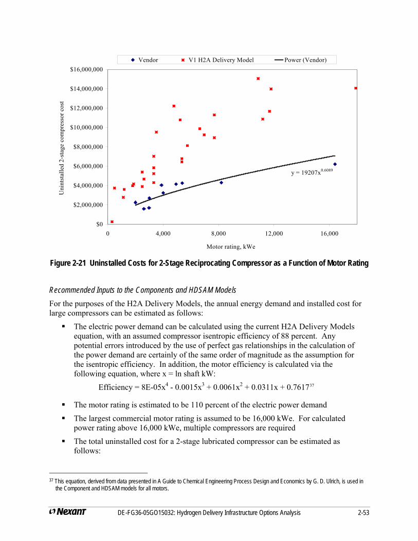
DE-FG36-05GO15032: Hydrogen Delivery Infrastructure Options Analysis 2-53
y = 19207x0.6089
$0
$2,000,000
$4,000,000
$6,000,000
$8,000,000
$10,000,000
$12,000,000
$14,000,000
$16,000,000
0 4,000 8,000 12,000 16,000
Motor rating, kWe
Uni
ntst
alle
d 2-
stag
e co
mpr
esso
r cos
t Vendor V1 H2A Delivery Model Power (Vendor)
Figure 2-21 Uninstalled Costs for 2-Stage Reciprocating Compressor as a Function of Motor Rating
Recommended Inputs to the Components and HDSAM Models For the purposes of the H2A Delivery Models, the annual energy demand and installed cost for large compressors can be estimated as follows:
The electric power demand can be calculated using the current H2A Delivery Models equation, with an assumed compressor isentropic efficiency of 88 percent. Any potential errors introduced by the use of perfect gas relationships in the calculation of the power demand are certainly of the same order of magnitude as the assumption for the isentropic efficiency. In addition, the motor efficiency is calculated via the following equation, where x = ln shaft kW:
Efficiency = 8E-05x4 - 0.0015x3 + 0.0061x2 + 0.0311x + 0.761737
The motor rating is estimated to be 110 percent of the electric power demand
The largest commercial motor rating is assumed to be 16,000 kWe. For calculated power rating above 16,000 kWe, multiple compressors are required
The total uninstalled cost for a 2-stage lubricated compressor can be estimated as follows:
37 This equation, derived from data presented in A Guide to Chemical Engineering Process Design and Economics by G. D. Ulrich, is used in
the Component and HDSAM models for all motors.
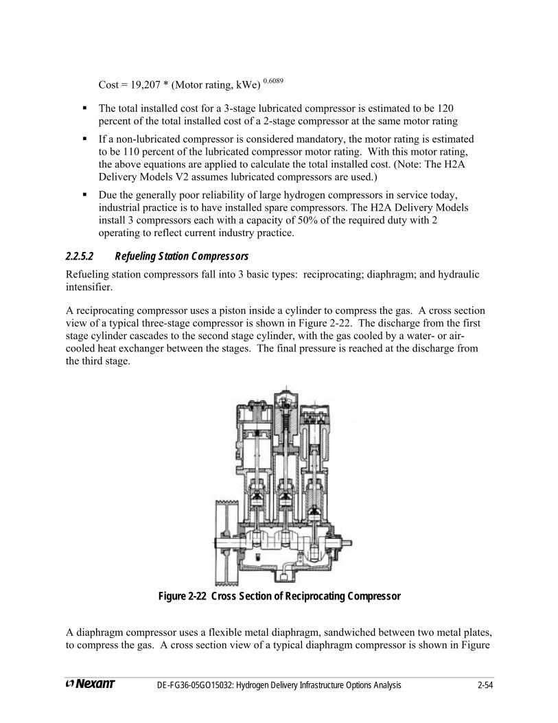
Cost = 19,207 * (Motor rating, kWe) 0.6089
The total installed cost for a 3-stage lubricated compressor is estimated to be 120 percent of the total installed cost of a 2-stage compressor at the same motor rating
If a non-lubricated compressor is considered mandatory, the motor rating is estimated to be 110 percent of the lubricated compressor motor rating. With this motor rating, the above equations are applied to calculate the total installed cost. (Note: The H2A Delivery Models V2 assumes lubricated compressors are used.)
Due the generally poor reliability of large hydrogen compressors in service today, industrial practice is to have installed spare compressors. The H2A Delivery Models install 3 compressors each with a capacity of 50% of the required duty with 2 operating to reflect current industry practice.
2.2.5.2 Refueling Station Compressors Refueling station compressors fall into 3 basic types: reciprocating; diaphragm; and hydraulic intensifier.
A reciprocating compressor uses a piston inside a cylinder to compress the gas. A cross section view of a typical three-stage compressor is shown in Figure 2-22. The discharge from the first stage cylinder cascades to the second stage cylinder, with the gas cooled by a water- or air-cooled heat exchanger between the stages. The final pressure is reached at the discharge from the third stage.
Figure 2-22 Cross Section of Reciprocating Compressor
A diaphragm compressor uses a flexible metal diaphragm, sandwiched between two metal plates, to compress the gas. A cross section view of a typical diaphragm compressor is shown in Figure
DE-FG36-05GO15032: Hydrogen Delivery Infrastructure Options Analysis 2-54
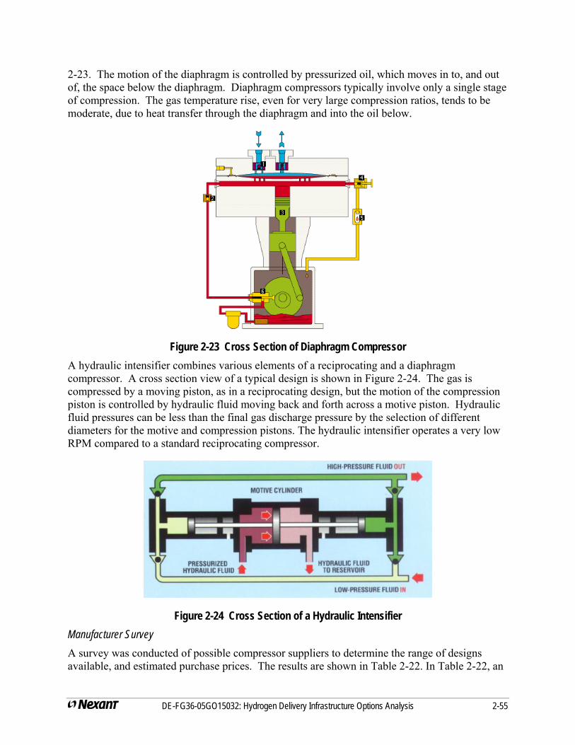
2-23. The motion of the diaphragm is controlled by pressurized oil, which moves in to, and out of, the space below the diaphragm. Diaphragm compressors typically involve only a single stage of compression. The gas temperature rise, even for very large compression ratios, tends to be moderate, due to heat transfer through the diaphragm and into the oil below.
Figure 2-23 Cross Section of Diaphragm Compressor A hydraulic intensifier combines various elements of a reciprocating and a diaphragm compressor. A cross section view of a typical design is shown in Figure 2-24. The gas is compressed by a moving piston, as in a reciprocating design, but the motion of the compression piston is controlled by hydraulic fluid moving back and forth across a motive piston. Hydraulic fluid pressures can be less than the final gas discharge pressure by the selection of different diameters for the motive and compression pistons. The hydraulic intensifier operates a very low RPM compared to a standard reciprocating compressor.
Figure 2-24 Cross Section of a Hydraulic Intensifier Manufacturer Survey A survey was conducted of possible compressor suppliers to determine the range of designs available, and estimated purchase prices. The results are shown in Table 2-22. In Table 2-22, an
DE-FG36-05GO15032: Hydrogen Delivery Infrastructure Options Analysis 2-55

allowance of 3 to 7 percent of the purchase price was added to the reciprocating compressors costs for an oil removal system following the last stage.
In general, the three types of compressors can meet the pressure requirements for a refueling station; specifically, an inlet pressure as low as 300 psi and a discharge pressure of 6,250 psi. However, as discussed in Section 2.1.3, refueling station capacities span the range of 50 kg/day to 6,000 kg/day in the H2A Delivery Models. Further, as discussed in Section 2.3, the optimum peak-to-average capacity ratio for the compressor is nominally 2.0. As such, the required range of compressor capacities is 8 kg/hr to 500 kg/hr. The largest compressor capacity identified in the survey was 250 kg/hr, which implies multiple compressors will be required for the larger refueling stations.
Compressor efficiencies were, in general, not supplied by the vendors. Further, calculating efficiency from the motor horsepower ratings can often lead to low calculated values. For the purposes of the H2A Delivery Models, a universal efficiency of 65 percent has been assumed for all refueling station compressor types and capacities.
Table 2-22 Results from Survey of Potential Refueling Station Compressors
Manufacturer Type Stages Capacity (kg/hr)
Inlet Pressure (psig)
Outlet Pressure
(psig)
Motor (HP)
Power (kW)
Comp. Cost ($K)
Filter Costs** ($K)
Uninstalled Costs ($K)
RIX* Recip 8.5 40 5500 81 2 83Knox-Western* Recip 28 144 6 150
RIX* Recip 42 40 4500 184 8 192Greenfield* Recip 42 35 4500 207 8 215Greenfield Recip 3 87 300 6000 250 265 17 282
Greenfield Recip 4 93 300 6000 250 265 19 284
RIX Recip 171 300 6500 1000 34 1034Knox-Western Recip 251 300 6500 900 50 950PDC Machines Diaphragm 2 50 300 6000 180 0 180PDC Machines Diaphragm 2 100 300 6000 385 0 385PDC Machines Diaphragm 2 164 300 6000 790 0 790
Fluitron Diaphragm 2 50 300 6000 100 43 155 0 155
PPI Diaphragm 2 33 300 6500 170 0 170
Hofer***(Neuman-Esser in U.S.)
Diaphragm 2 50 300 6000 125 350 0 350
Hydro-Pac Intensifier 2 9.2 300 6000 60 35 73 29 102Hydro-Pac**** Intensifier 1 30 6250 12500 40 70 7 77
* The costs here are 15% greater than quoted costs to reflect the difference in the inlet/outlet pressure per recommendation of David Savidge, RIX ** Additional filtration (10% of compressor cost) is added to reciprocating compressors *** This data point not considered as it appears to be a statistical outlier and comes from and unofficial quote. **** This Hydro-Pac compressor was not considered in the cost estimation as it is significantly outside the pressure range required in the forecourt
DE-FG36-05GO15032: Hydrogen Delivery Infrastructure Options Analysis 2-56
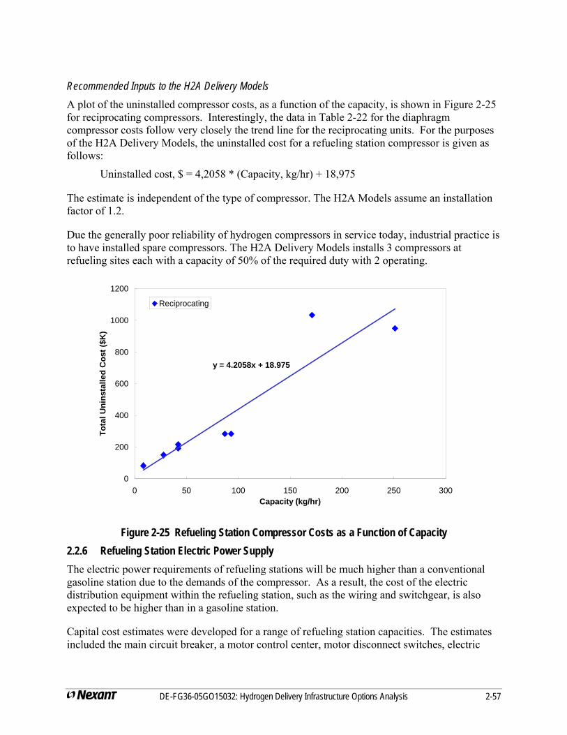
Recommended Inputs to the H2A Delivery Models A plot of the uninstalled compressor costs, as a function of the capacity, is shown in Figure 2-25 for reciprocating compressors. Interestingly, the data in Table 2-22 for the diaphragm compressor costs follow very closely the trend line for the reciprocating units. For the purposes of the H2A Delivery Models, the uninstalled cost for a refueling station compressor is given as follows:
Uninstalled cost, $ = 4,2058 * (Capacity, kg/hr) + 18,975
The estimate is independent of the type of compressor. The H2A Models assume an installation factor of 1.2.
Due the generally poor reliability of hydrogen compressors in service today, industrial practice is to have installed spare compressors. The H2A Delivery Models installs 3 compressors at refueling sites each with a capacity of 50% of the required duty with 2 operating.
y = 4.2058x + 18.975
0
200
400
600
800
1000
1200
0 50 100 150 200 250 300Capacity (kg/hr)
Tota
l Uni
nsta
lled
Cos
t ($K
)
Reciprocating
Figure 2-25 Refueling Station Compressor Costs as a Function of Capacity 2.2.6 Refueling Station Electric Power Supply The electric power requirements of refueling stations will be much higher than a conventional gasoline station due to the demands of the compressor. As a result, the cost of the electric distribution equipment within the refueling station, such as the wiring and switchgear, is also expected to be higher than in a gasoline station.
Capital cost estimates were developed for a range of refueling station capacities. The estimates included the main circuit breaker, a motor control center, motor disconnect switches, electric
DE-FG36-05GO15032: Hydrogen Delivery Infrastructure Options Analysis 2-57
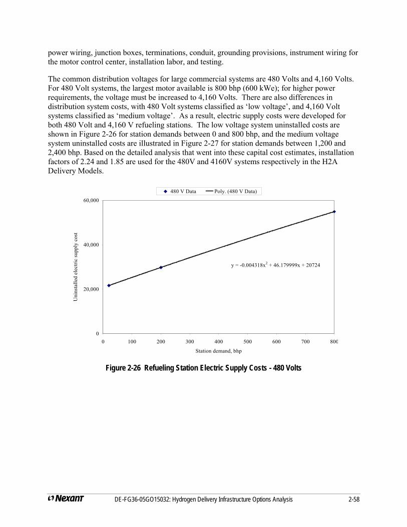
power wiring, junction boxes, terminations, conduit, grounding provisions, instrument wiring for the motor control center, installation labor, and testing.
The common distribution voltages for large commercial systems are 480 Volts and 4,160 Volts. For 480 Volt systems, the largest motor available is 800 bhp (600 kWe); for higher power requirements, the voltage must be increased to 4,160 Volts. There are also differences in distribution system costs, with 480 Volt systems classified as ‘low voltage’, and 4,160 Volt systems classified as ‘medium voltage’. As a result, electric supply costs were developed for both 480 Volt and 4,160 V refueling stations. The low voltage system uninstalled costs are shown in Figure 2-26 for station demands between 0 and 800 bhp, and the medium voltage system uninstalled costs are illustrated in Figure 2-27 for station demands between 1,200 and 2,400 bhp. Based on the detailed analysis that went into these capital cost estimates, installation factors of 2.24 and 1.85 are used for the 480V and 4160V systems respectively in the H2A Delivery Models.
y = -0.004318x2 + 46.179999x + 20724
0
20,000
40,000
60,000
0 100 200 300 400 500 600 700 800
Station demand, bhp
Uni
nsta
lled
elec
tric
supp
ly c
ost
480 V Data Poly. (480 V Data)
Figure 2-26 Refueling Station Electric Supply Costs - 480 Volts
DE-FG36-05GO15032: Hydrogen Delivery Infrastructure Options Analysis 2-58
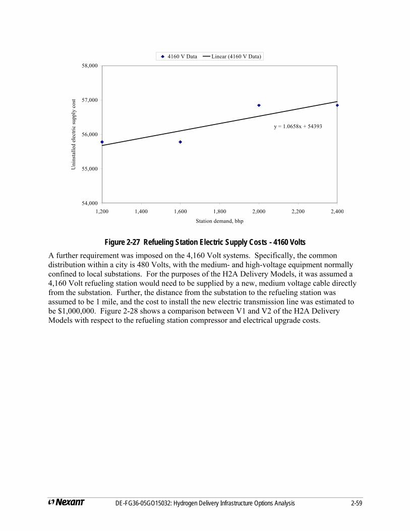
y = 1.0658x + 54393
54,000
55,000
56,000
57,000
58,000
1,200 1,400 1,600 1,800 2,000 2,200 2,400
Station demand, bhp
Uni
nsta
lled
elec
tric
supp
ly c
ost
4160 V Data Linear (4160 V Data)
Figure 2-27 Refueling Station Electric Supply Costs - 4160 Volts A further requirement was imposed on the 4,160 Volt systems. Specifically, the common distribution within a city is 480 Volts, with the medium- and high-voltage equipment normally confined to local substations. For the purposes of the H2A Delivery Models, it was assumed a 4,160 Volt refueling station would need to be supplied by a new, medium voltage cable directly from the substation. Further, the distance from the substation to the refueling station was assumed to be 1 mile, and the cost to install the new electric transmission line was estimated to be $1,000,000. Figure 2-28 shows a comparison between V1 and V2 of the H2A Delivery Models with respect to the refueling station compressor and electrical upgrade costs.
DE-FG36-05GO15032: Hydrogen Delivery Infrastructure Options Analysis 2-59
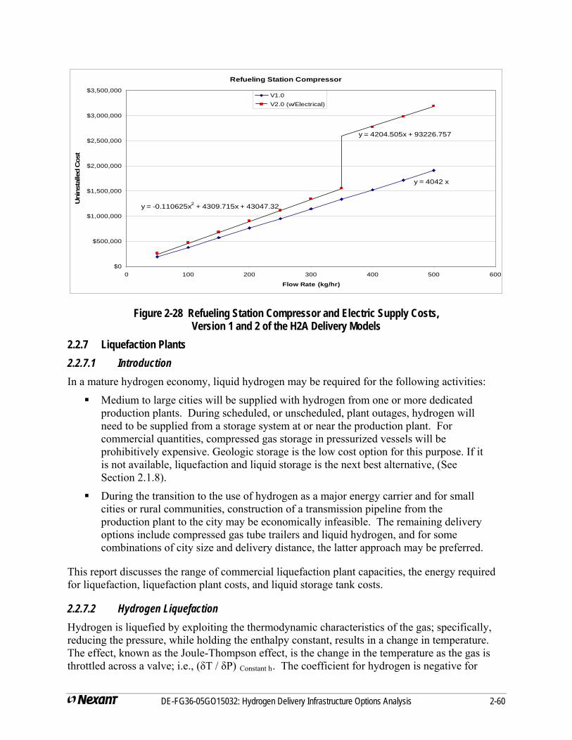
Refueling Station Compressor
$0
$500,000
$1,000,000
$1,500,000
$2,000,000
$2,500,000
$3,000,000
$3,500,000
0 100 200 300 400 500 600
Flow Rate (kg/hr)
Uni
nsta
lled
Cos
t
V1.0V2.0 (w/Electrical)
y = 4042 x
y = -0.110625x2 + 4309.715x + 43047.32
y = 4204.505x + 93226.757
Figure 2-28 Refueling Station Compressor and Electric Supply Costs, Version 1 and 2 of the H2A Delivery Models
2.2.7 Liquefaction Plants 2.2.7.1 Introduction In a mature hydrogen economy, liquid hydrogen may be required for the following activities:
Medium to large cities will be supplied with hydrogen from one or more dedicated production plants. During scheduled, or unscheduled, plant outages, hydrogen will need to be supplied from a storage system at or near the production plant. For commercial quantities, compressed gas storage in pressurized vessels will be prohibitively expensive. Geologic storage is the low cost option for this purpose. If it is not available, liquefaction and liquid storage is the next best alternative, (See Section 2.1.8).
During the transition to the use of hydrogen as a major energy carrier and for small cities or rural communities, construction of a transmission pipeline from the production plant to the city may be economically infeasible. The remaining delivery options include compressed gas tube trailers and liquid hydrogen, and for some combinations of city size and delivery distance, the latter approach may be preferred.
This report discusses the range of commercial liquefaction plant capacities, the energy required for liquefaction, liquefaction plant costs, and liquid storage tank costs.
2.2.7.2 Hydrogen Liquefaction Hydrogen is liquefied by exploiting the thermodynamic characteristics of the gas; specifically, reducing the pressure, while holding the enthalpy constant, results in a change in temperature. The effect, known as the Joule-Thompson effect, is the change in the temperature as the gas is throttled across a valve; i.e., (δT / δP) Constant h. The coefficient for hydrogen is negative for
DE-FG36-05GO15032: Hydrogen Delivery Infrastructure Options Analysis 2-60
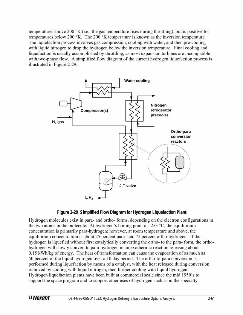
temperatures above 200 °K (i.e., the gas temperature rises during throttling), but is positive for temperatures below 200 °K. The 200 °K temperature is known as the inversion temperature. The liquefaction process involves gas compression, cooling with water, and then pre-cooling with liquid nitrogen to drop the hydrogen below the inversion temperature. Final cooling and liquefaction is usually accomplished by throttling, as most expansion turbines are incompatible with two-phase flow. A simplified flow diagram of the current hydrogen liquefaction process is illustrated in Figure 2-29.
Water cooling
Nitrogen refrigerator precooler
Ortho-para conversion reactors
J-T valve
L H2
H2 gas
Compressor(s)
Figure 2-29 Simplified Flow Diagram for Hydrogen Liquefaction Plant Hydrogen molecules exist in para- and ortho- forms, depending on the electron configurations in the two atoms in the molecule. At hydrogen’s boiling point of -253 °C, the equilibrium concentration is primarily para-hydrogen; however, at room temperature and above, the equilibrium concentration is about 25 percent para- and 75 percent ortho-hydrogen. If the hydrogen is liquefied without first catalytically converting the ortho- to the para- form, the ortho-hydrogen will slowly convert to para-hydrogen in an exothermic reaction releasing about 0.15 kWh/kg of energy. The heat of transformation can cause the evaporation of as much as 50 percent of the liquid hydrogen over a 10 day period. The ortho-to-para conversion is performed during liquefaction by means of a catalyst, with the heat released during conversion removed by cooling with liquid nitrogen, then further cooling with liquid hydrogen. Hydrogen liquefaction plants have been built at commercial scale since the mid 1950’s to support the space program and to support other uses of hydrogen such as in the specialty
DE-FG36-05GO15032: Hydrogen Delivery Infrastructure Options Analysis 2-61
chemical industries and in the electronics industry. A large plant was built in Florida with a capacity of 30 metric tons/day, and other large plants followed in the 1960’s to support the Apollo program. There are currently 10 plants in the US with capacities ranging from 5.4 to 32 metric tons per day. However, activity in new plant construction has been quiet in the last few years. Recent plants built in Japan and Europe are in the 5 metric ton per day range.
Discussions were held with Andres Kundig of Linde Kryotechnik AG in Switzerland regarding existing, and planned, liquefaction plants. The largest single train plant built by Linde is a 13.5 metric ton per day unit in Magog, Canada. The current limitations on train size are the aluminum plate fin exchangers, the cold box diameter, and the desire to shop fabricate, as opposed to field fabricate the equipment. The current largest size of the cold box is around 15 metric tons per day. A 50 metric ton per day plant has been planned, which would use 3 cold boxes. For a 50 metric ton per day plant, there are 4 expansion turbines in the nitrogen loop, and 6 expansion turbines in the hydrogen loop.
In the future, if there is a demand for a large, single-train plant, Mr. Kundig could foresee new manufacturing techniques that would increase the largest capacity which can be shop fabricated; alternately, larger units would need to be field fabricated. He believes a 250 to 300 metric ton per day plant could be built, but no one has studied this in detail. Other industrial gas hydrogen suppliers have suggested that 100 metric tons per day might be the largest practical size. We have elected to limit the maximum size in the H2A Delivery Models V2 to 200 metric tons/day. Multiple units are used if demand exceeds this.
The hydrogen supplied to a liquefaction plant is typically 99.999 percent hydrogen. Due to the high purity of the feed stream, Linde states the liquefaction plant should be available for at least 360 days each year (98.6 percent availability).
2.2.7.3 Liquefaction Plant Energy Consumption The liquefier efficiency is often characterized as the input work required for producing a unit mass of liquid. The ideal work, with zero thermodynamic irreversibility, is a two-step process, involving isothermal compression, followed by isentropic expansion to the liquid state. The theoretical work to liquefy hydrogen from ambient conditions, including the ortho-to-para conversion, is approximately 3.9 kWh/kg.
Currently, Linde has two plants which produce 4.4 and 13.5 metric tons per day in Ingolstadt, Germany, and Magog, Canada, respectively. The smaller plant has an electric consumption of 13 kWh/kg of hydrogen, and the larger one, 12 kWh/kg. Both plants were built in the early 1990’s. Linde feels that with the best current compressor technology, a new 10 metric ton per day plant could have an energy requirement of 10 kWh/kg, and a 50 metric ton per day plant, 9 kWh/kg. In the future, Linde predicts the energy demand could be reduced to 8 kWh/kg. These values assume the hydrogen is supplied from a plant at a pressure of 18 bars.
Air Liquide operates a 10 metric ton per day liquefaction plant, which has a unit energy demand of approximately 18 kWh/kg. However, the plant has been in operation for many years, and a current design would have a lower energy consumption. Air Liquide believes the lower limit on the liquefaction energy to be one-half of that in their present plant.
DE-FG36-05GO15032: Hydrogen Delivery Infrastructure Options Analysis 2-62
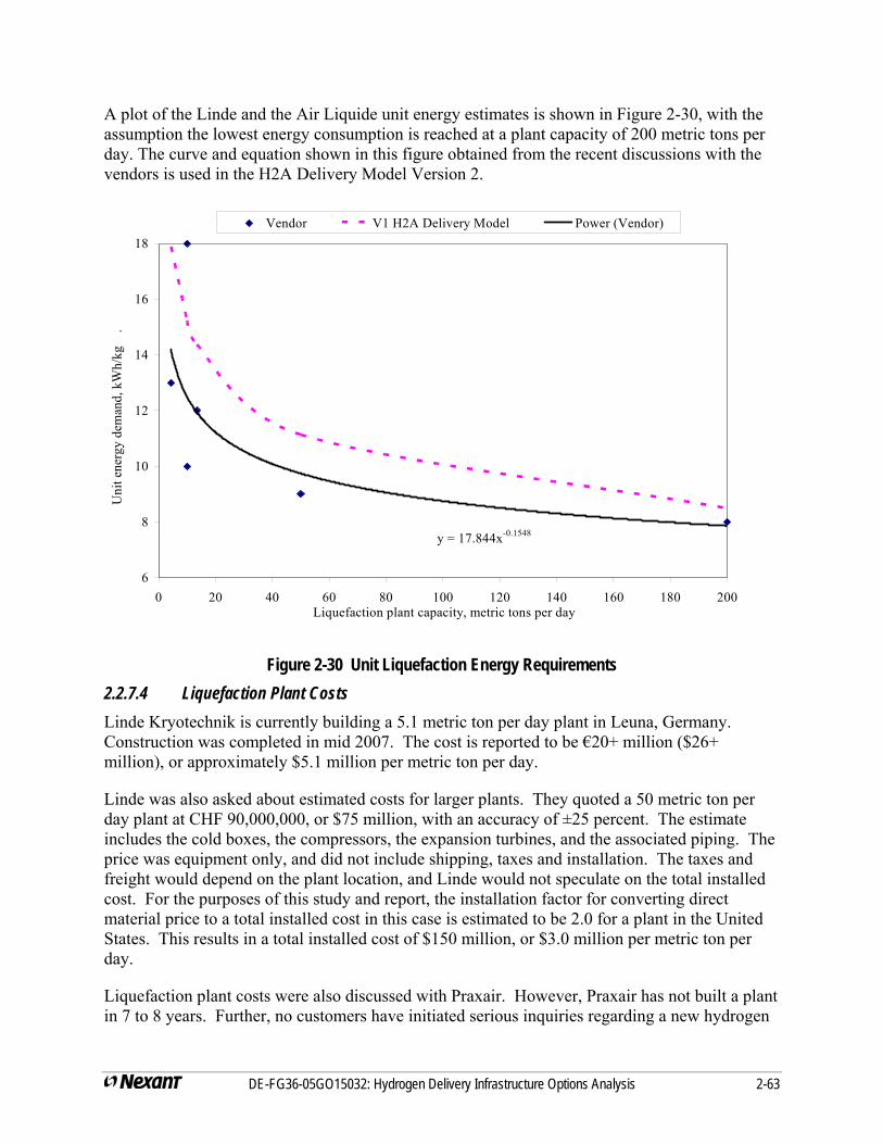
A plot of the Linde and the Air Liquide unit energy estimates is shown in Figure 2-30, with the assumption the lowest energy consumption is reached at a plant capacity of 200 metric tons per day. The curve and equation shown in this figure obtained from the recent discussions with the vendors is used in the H2A Delivery Model Version 2.
y = 17.844x-0.1548
6
8
10
12
14
16
18
0 20 40 60 80 100 120 140 160 180 200Liquefaction plant capacity, metric tons per day
Uni
t ene
rgy
dem
and,
kW
h/kg
.
Vendor V1 H2A Delivery Model Power (Vendor)
Figure 2-30 Unit Liquefaction Energy Requirements 2.2.7.4 Liquefaction Plant Costs Linde Kryotechnik is currently building a 5.1 metric ton per day plant in Leuna, Germany. Construction was completed in mid 2007. The cost is reported to be €20+ million ($26+ million), or approximately $5.1 million per metric ton per day.
Linde was also asked about estimated costs for larger plants. They quoted a 50 metric ton per day plant at CHF 90,000,000, or $75 million, with an accuracy of ±25 percent. The estimate includes the cold boxes, the compressors, the expansion turbines, and the associated piping. The price was equipment only, and did not include shipping, taxes and installation. The taxes and freight would depend on the plant location, and Linde would not speculate on the total installed cost. For the purposes of this study and report, the installation factor for converting direct material price to a total installed cost in this case is estimated to be 2.0 for a plant in the United States. This results in a total installed cost of $150 million, or $3.0 million per metric ton per day.
Liquefaction plant costs were also discussed with Praxair. However, Praxair has not built a plant in 7 to 8 years. Further, no customers have initiated serious inquiries regarding a new hydrogen
DE-FG36-05GO15032: Hydrogen Delivery Infrastructure Options Analysis 2-63
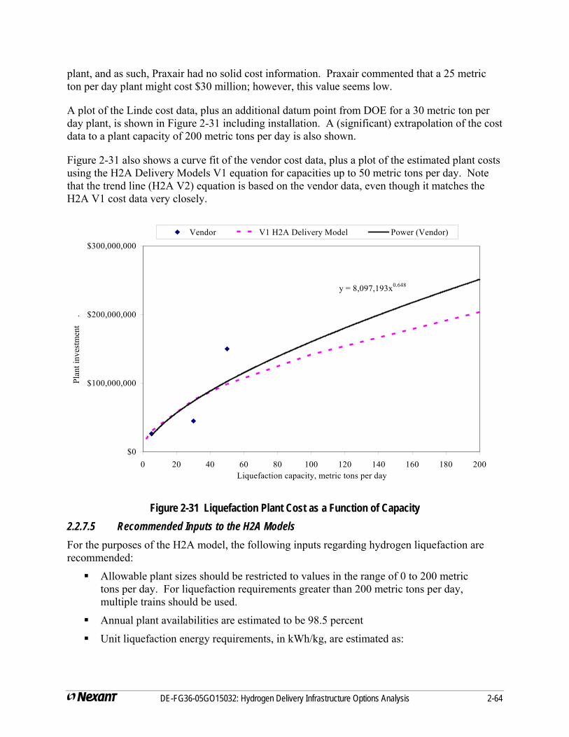
plant, and as such, Praxair had no solid cost information. Praxair commented that a 25 metric ton per day plant might cost $30 million; however, this value seems low.
A plot of the Linde cost data, plus an additional datum point from DOE for a 30 metric ton per day plant, is shown in Figure 2-31 including installation. A (significant) extrapolation of the cost data to a plant capacity of 200 metric tons per day is also shown.
Figure 2-31 also shows a curve fit of the vendor cost data, plus a plot of the estimated plant costs using the H2A Delivery Models V1 equation for capacities up to 50 metric tons per day. Note that the trend line (H2A V2) equation is based on the vendor data, even though it matches the H2A V1 cost data very closely.
y = 8,097,193x0.648
$0
$100,000,000
$200,000,000
$300,000,000
0 20 40 60 80 100 120 140 160 180 200Liquefaction capacity, metric tons per day
Plan
t inv
estm
ent
.
Vendor V1 H2A Delivery Model Power (Vendor)
Figure 2-31 Liquefaction Plant Cost as a Function of Capacity 2.2.7.5 Recommended Inputs to the H2A Models For the purposes of the H2A model, the following inputs regarding hydrogen liquefaction are recommended:
Allowable plant sizes should be restricted to values in the range of 0 to 200 metric tons per day. For liquefaction requirements greater than 200 metric tons per day, multiple trains should be used.
Annual plant availabilities are estimated to be 98.5 percent
Unit liquefaction energy requirements, in kWh/kg, are estimated as:
DE-FG36-05GO15032: Hydrogen Delivery Infrastructure Options Analysis 2-64
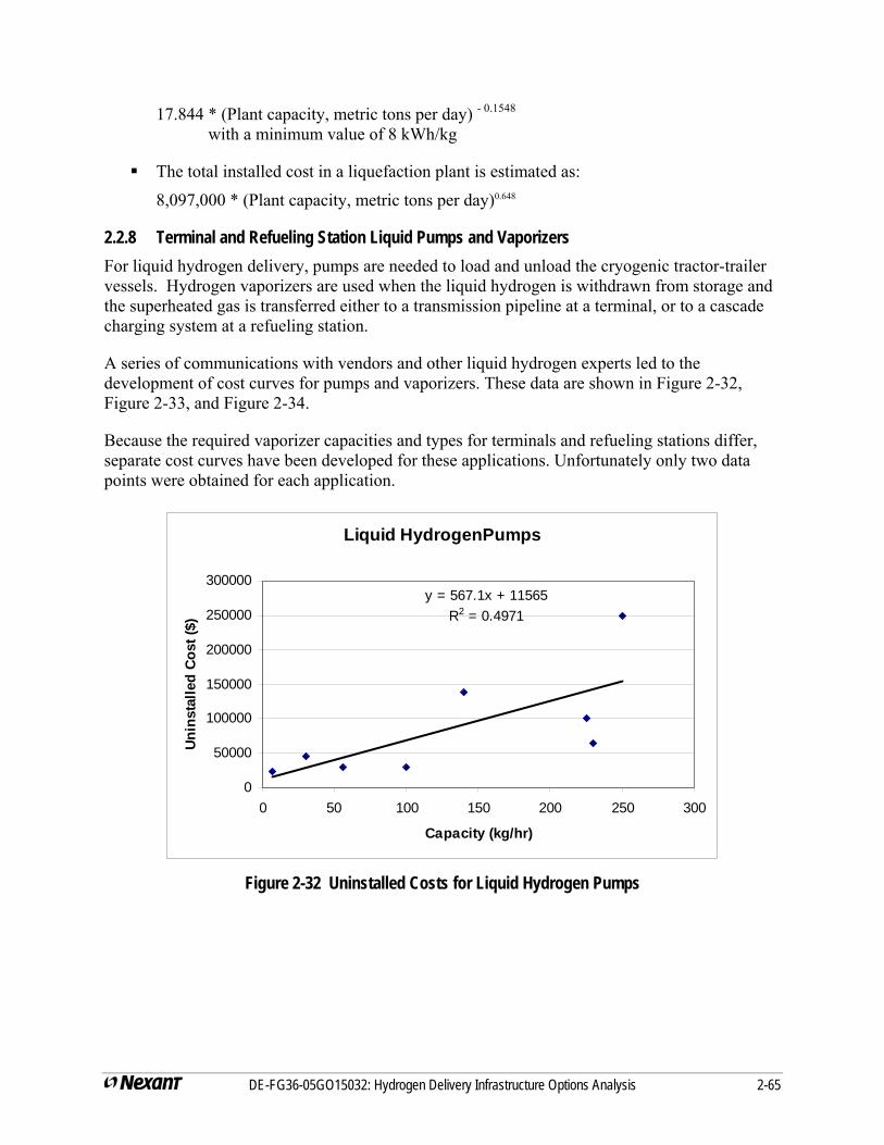
17.844 * (Plant capacity, metric tons per day) - 0.1548
with a minimum value of 8 kWh/kg
The total installed cost in a liquefaction plant is estimated as:
8,097,000 * (Plant capacity, metric tons per day)0.648
2.2.8 Terminal and Refueling Station Liquid Pumps and Vaporizers For liquid hydrogen delivery, pumps are needed to load and unload the cryogenic tractor-trailer vessels. Hydrogen vaporizers are used when the liquid hydrogen is withdrawn from storage and the superheated gas is transferred either to a transmission pipeline at a terminal, or to a cascade charging system at a refueling station.
A series of communications with vendors and other liquid hydrogen experts led to the development of cost curves for pumps and vaporizers. These data are shown in Figure 2-32, Figure 2-33, and Figure 2-34.
Because the required vaporizer capacities and types for terminals and refueling stations differ, separate cost curves have been developed for these applications. Unfortunately only two data points were obtained for each application.
Liquid HydrogenPumps
y = 567.1x + 11565R2 = 0.4971
0
50000
100000
150000
200000
250000
300000
0 50 100 150 200 250 300
Capacity (kg/hr)
Unin
stal
led
Cost
($)
Figure 2-32 Uninstalled Costs for Liquid Hydrogen Pumps
DE-FG36-05GO15032: Hydrogen Delivery Infrastructure Options Analysis 2-65
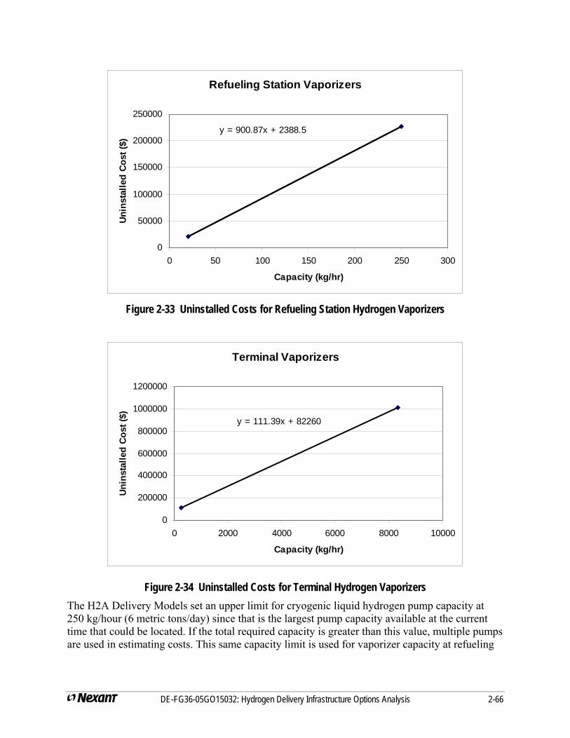
Refueling Station Vaporizers
y = 900.87x + 2388.5
0
50000
100000
150000
200000
250000
0 50 100 150 200 250 300
Capacity (kg/hr)
Unin
stal
led
Cost
($)
Figure 2-33 Uninstalled Costs for Refueling Station Hydrogen Vaporizers
Terminal Vaporizers
y = 111.39x + 82260
0
200000
400000
600000
800000
1000000
1200000
0 2000 4000 6000 8000 10000
Capacity (kg/hr)
Uni
nsta
lled
Cos
t ($)
Figure 2-34 Uninstalled Costs for Terminal Hydrogen Vaporizers The H2A Delivery Models set an upper limit for cryogenic liquid hydrogen pump capacity at 250 kg/hour (6 metric tons/day) since that is the largest pump capacity available at the current time that could be located. If the total required capacity is greater than this value, multiple pumps are used in estimating costs. This same capacity limit is used for vaporizer capacity at refueling
DE-FG36-05GO15032: Hydrogen Delivery Infrastructure Options Analysis 2-66
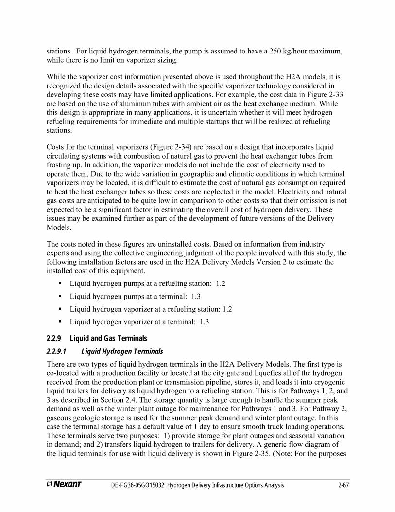
stations. For liquid hydrogen terminals, the pump is assumed to have a 250 kg/hour maximum, while there is no limit on vaporizer sizing.
While the vaporizer cost information presented above is used throughout the H2A models, it is recognized the design details associated with the specific vaporizer technology considered in developing these costs may have limited applications. For example, the cost data in Figure 2-33 are based on the use of aluminum tubes with ambient air as the heat exchange medium. While this design is appropriate in many applications, it is uncertain whether it will meet hydrogen refueling requirements for immediate and multiple startups that will be realized at refueling stations.
Costs for the terminal vaporizers (Figure 2-34) are based on a design that incorporates liquid circulating systems with combustion of natural gas to prevent the heat exchanger tubes from frosting up. In addition, the vaporizer models do not include the cost of electricity used to operate them. Due to the wide variation in geographic and climatic conditions in which terminal vaporizers may be located, it is difficult to estimate the cost of natural gas consumption required to heat the heat exchanger tubes so these costs are neglected in the model. Electricity and natural gas costs are anticipated to be quite low in comparison to other costs so that their omission is not expected to be a significant factor in estimating the overall cost of hydrogen delivery. These issues may be examined further as part of the development of future versions of the Delivery Models.
The costs noted in these figures are uninstalled costs. Based on information from industry experts and using the collective engineering judgment of the people involved with this study, the following installation factors are used in the H2A Delivery Models Version 2 to estimate the installed cost of this equipment.
Liquid hydrogen pumps at a refueling station: 1.2
Liquid hydrogen pumps at a terminal: 1.3
Liquid hydrogen vaporizer at a refueling station: 1.2
Liquid hydrogen vaporizer at a terminal: 1.3
2.2.9 Liquid and Gas Terminals 2.2.9.1 Liquid Hydrogen Terminals There are two types of liquid hydrogen terminals in the H2A Delivery Models. The first type is co-located with a production facility or located at the city gate and liquefies all of the hydrogen received from the production plant or transmission pipeline, stores it, and loads it into cryogenic liquid trailers for delivery as liquid hydrogen to a refueling station. This is for Pathways 1, 2, and 3 as described in Section 2.4. The storage quantity is large enough to handle the summer peak demand as well as the winter plant outage for maintenance for Pathways 1 and 3. For Pathway 2, gaseous geologic storage is used for the summer peak demand and winter plant outage. In this case the terminal storage has a default value of 1 day to ensure smooth truck loading operations. These terminals serve two purposes: 1) provide storage for plant outages and seasonal variation in demand; and 2) transfers liquid hydrogen to trailers for delivery. A generic flow diagram of the liquid terminals for use with liquid delivery is shown in Figure 2-35. (Note: For the purposes
DE-FG36-05GO15032: Hydrogen Delivery Infrastructure Options Analysis 2-67
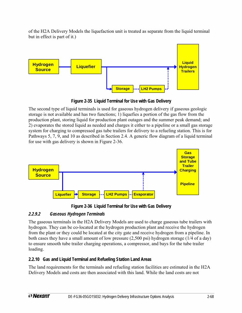
of the H2A Delivery Models the liquefaction unit is treated as separate from the liquid terminal but in effect is part of it.)
Hydrogen Source
Storage LH2 Pumps
Liquid Hydrogen Trailers
Liquefier
Figure 2-35 Liquid Terminal for Use with Gas Delivery The second type of liquid terminals is used for gaseous hydrogen delivery if gaseous geologic storage is not available and has two functions; 1) liquefies a portion of the gas flow from the production plant, storing liquid for production plant outages and the summer peak demand; and 2) evaporates the stored liquid as needed and charges it either to a pipeline or a small gas storage system for charging to compressed gas tube trailers for delivery to a refueling station. This is for Pathways 5, 7, 9, and 10 as described in Section 2.4. A generic flow diagram of a liquid terminal for use with gas delivery is shown in Figure 2-36.
Hydrogen Source
Liquefier Storage LH2 Pumps Evaporator
Gas Storage
and Tube Trailer
Charging
Pipeline
Figure 2-36 Liquid Terminal for Use with Gas Delivery 2.2.9.2 Gaseous Hydrogen Terminals The gaseous terminals in the H2A Delivery Models are used to charge gaseous tube trailers with hydrogen. They can be co-located at the hydrogen production plant and receive the hydrogen from the plant or they could be located at the city gate and receive hydrogen from a pipeline. In both cases they have a small amount of low pressure (2,500 psi) hydrogen storage (1/4 of a day) to ensure smooth tube trailer charging operations, a compressor, and bays for the tube trailer loading.
2.2.10 Gas and Liquid Terminal and Refueling Station Land Areas The land requirements for the terminals and refueling station facilities are estimated in the H2A Delivery Models and costs are then associated with this land. While the land costs are not
DE-FG36-05GO15032: Hydrogen Delivery Infrastructure Options Analysis 2-68
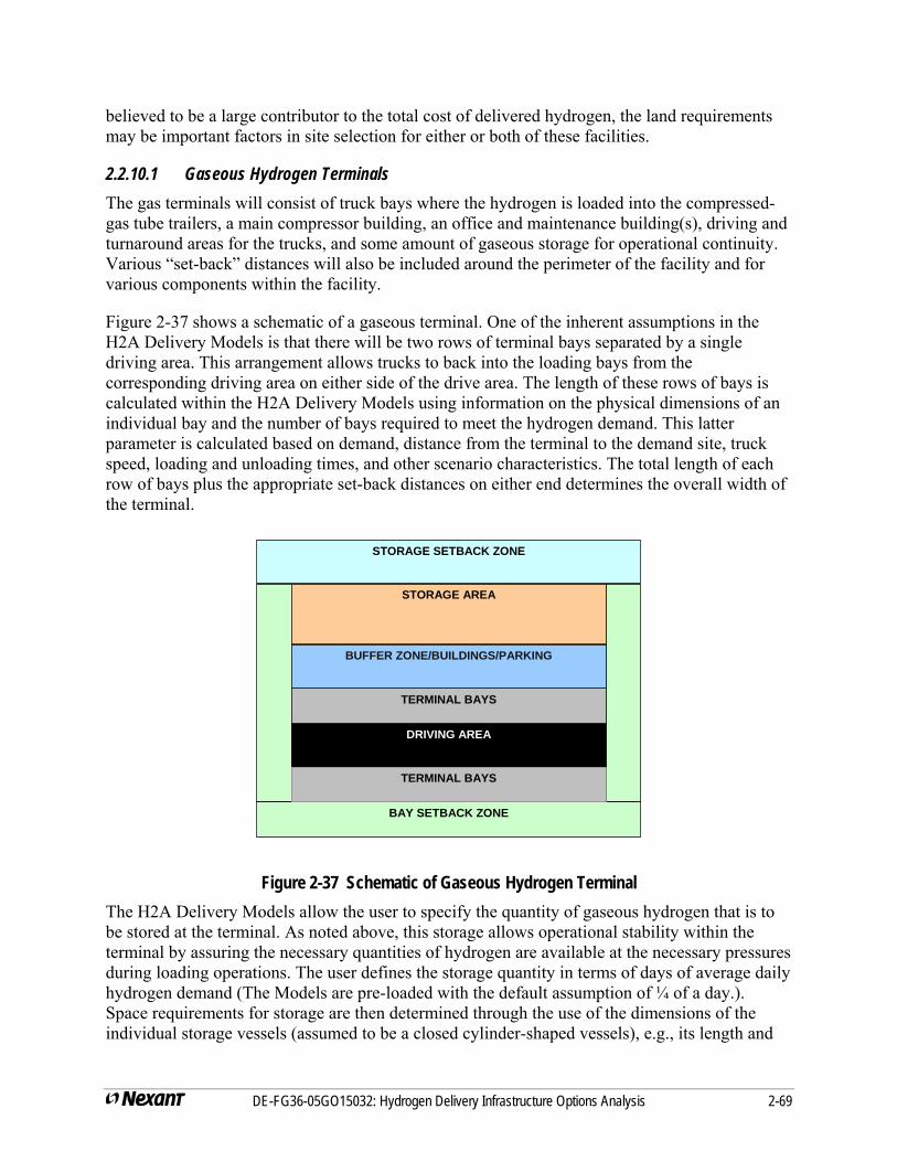
believed to be a large contributor to the total cost of delivered hydrogen, the land requirements may be important factors in site selection for either or both of these facilities.
2.2.10.1 Gaseous Hydrogen Terminals The gas terminals will consist of truck bays where the hydrogen is loaded into the compressed-gas tube trailers, a main compressor building, an office and maintenance building(s), driving and turnaround areas for the trucks, and some amount of gaseous storage for operational continuity. Various “set-back” distances will also be included around the perimeter of the facility and for various components within the facility.
Figure 2-37 shows a schematic of a gaseous terminal. One of the inherent assumptions in the H2A Delivery Models is that there will be two rows of terminal bays separated by a single driving area. This arrangement allows trucks to back into the loading bays from the corresponding driving area on either side of the drive area. The length of these rows of bays is calculated within the H2A Delivery Models using information on the physical dimensions of an individual bay and the number of bays required to meet the hydrogen demand. This latter parameter is calculated based on demand, distance from the terminal to the demand site, truck speed, loading and unloading times, and other scenario characteristics. The total length of each row of bays plus the appropriate set-back distances on either end determines the overall width of the terminal.
DRIVING AREA
BAY SETBACK ZONE
TERMINAL BAYS
TERMINAL BAYS
BUFFER ZONE/BUILDINGS/PARKING
STORAGE AREA
STORAGE SETBACK ZONE
Figure 2-37 Schematic of Gaseous Hydrogen Terminal The H2A Delivery Models allow the user to specify the quantity of gaseous hydrogen that is to be stored at the terminal. As noted above, this storage allows operational stability within the terminal by assuring the necessary quantities of hydrogen are available at the necessary pressures during loading operations. The user defines the storage quantity in terms of days of average daily hydrogen demand (The Models are pre-loaded with the default assumption of ¼ of a day.). Space requirements for storage are then determined through the use of the dimensions of the individual storage vessels (assumed to be a closed cylinder-shaped vessels), e.g., its length and
DE-FG36-05GO15032: Hydrogen Delivery Infrastructure Options Analysis 2-69
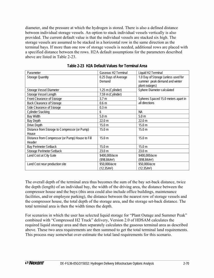
diameter, and the pressure at which the hydrogen is stored. There is also a defined distance between individual storage vessels. An option to stack individual vessels vertically is also provided. The current default value is that the individual vessels are stacked six high. The storage vessels are assumed to be stacked in a horizontal row in the same direction as the terminal bays. If more than one row of storage vessels is needed, additional rows are placed with a specified distance between the rows. H2A default assumptions for the parameters described above are listed in Table 2-23.
Table 2-23 H2A Default Values for Terminal Area Parameter Gaseous H2 Terminal Liquid H2 Terminal Storage Quantity 0.25 Days of Average
Demand 1.0 Day of Storage (unless used for summer peak demand and winter plant outages)
Storage Vessel Diameter 1.25 m (Cylinder) Sphere Diameter calculated Storage Vessel Length 7.59 m (Cylinder) Front Clearance of Storage 3.7 m Spheres Spaced 15.0 meters apart in
all directions Back Clearance of Storage 0.6 m Side Clearance of Storage 0.3 m Cylinder Stacking 6 NA Bay Width 5.0 m 5.0 m Bay Depth 22.0 m 22.0 m Drive Depth 15.0 m 15.0 m Distance from Storage to Compressor (or Pump) House
15.0 m 15.0 m
Distance from Compressor (or Pump) House to Fill Header
15.0 m 15.0 m
Bay Perimeter Setback 15.0 m 15.0 m Storage Perimeter Setback 23.0 m 23.0 m Land Cost at City Gate $400,000/acre
($98.84/m2) $400,000/acre ($98.84/m2)
Land Cost near production site $50,000/acre (12.35/m2)
$50,000/acre (12.35/m2)
The overall depth of the terminal area thus becomes the sum of the bay set-back distance, twice the depth (length) of an individual bay, the width of the driving area, the distance between the compressor house and the bays (this area could also include office buildings, maintenance facilities, and/or employee parking), the distance between the nearest row of storage vessels and the compressor house, the total depth of the storage area, and the storage set-back distance. The total terminal area is then the width times the depth.
For scenarios in which the user has selected liquid storage for “Plant Outage and Summer Peak” combined with “Compressed H2 Truck” delivery, Version 2.0 of HDSAM calculates the required liquid storage area and then separately calculates the gaseous terminal area as described above. These two area requirements are then summed to get the total terminal land requirements. This process may somewhat over-estimate the total land requirements for this scenario.
DE-FG36-05GO15032: Hydrogen Delivery Infrastructure Options Analysis 2-70

2.2.10.2 Liquid hydrogen Terminal Area requirements for a liquid terminal for the liquid delivery pathways using cryogenic liquid trucks is estimated in much the same way as for gaseous hydrogen terminals . As before, the width of the terminal is estimated as the length of a row of bays (plus set-back distances) containing half the total number of bays needed. The depth of the storage area is also determined in a manner similar to that for gaseous hydrogen storage except that it is assumed that each cryogenic storage vessel is a sphere capable of holding up to 3,500 cubic meters of liquid hydrogen. This size storage vessel is the largest for which information was available. The H2A Delivery Models determine the number of such storage vessels needed and locates them in a manner similar to that for the gaseous storage vessels. There is little available information regarding the physical dimensions of liquid hydrogen pumps and vaporizers of the scale needed for large-scale, long term storage. Therefore, Version 2.0 of the H2A Delivery Models does not estimate the land requirements for this equipment. Subsequent versions of the model will include such estimates. Default values used in the H2A Delivery Models for liquid terminals are also shown in Table 2-20A.
The second type of liquid terminal arises when the H2A Delivery Models user elects either the gaseous hydrogen truck or pipeline delivery pathway and also elects to provide long term storage in liquid hydrogen form. Such storage would be used to meet peak summer demand as well to meet hydrogen demand during the annually scheduled production-plant maintenance shutdown. Under this option a small quantity of the production stream is bled off, liquefied and stored in cryogenic, spherical tanks. This bleed stream is to provide sufficient hydrogen to meet the extra, summer demand as well as to meet the demand during the winter period when the production facility is shut down for maintenance (a default value of 10 days plant outage is used). The terminal equipment required when using liquid hydrogen storage in a gaseous hydrogen delivery pathway includes a liquefier, cryogenic storage vessels, liquid hydrogen pumps, and a hydrogen vaporizer.
Area requirements for this type of liquid hydrogen terminal are estimated in a manner similar to that for first type of liquid hydrogen terminal. A major difference however, is that no bays are required. Therefore the model defines the space requirements for the spherical cryogenic storage vessel(s) and assumes that these storage vessels are placed in a single row with the required set-back distances on either end and in front and back of the storage vessels. While this configuration is not likely to be exactly followed in an actual application, the estimation of the land requirement is believed to be representative of configurations that might be used in real applications.
One important difference in the land requirements for liquid terminal compared to gaseous terminals is that a liquid terminal requires a liquefier to be located with the terminal and land requirements for liquefiers are significant. The H2A Delivery Models estimates the liquefier land requirements by scaling to a 0.6 power a reference case value that a 30 metric ton/day hydrogen liquefier will occupy 25,000 square meters.
2.2.10.3 Refueling Station Land Areas In order to properly define the characteristics and costs of hydrogen delivery it is necessary to determine the land area required for a hydrogen fueling station. In order to determine the area
DE-FG36-05GO15032: Hydrogen Delivery Infrastructure Options Analysis 2-71
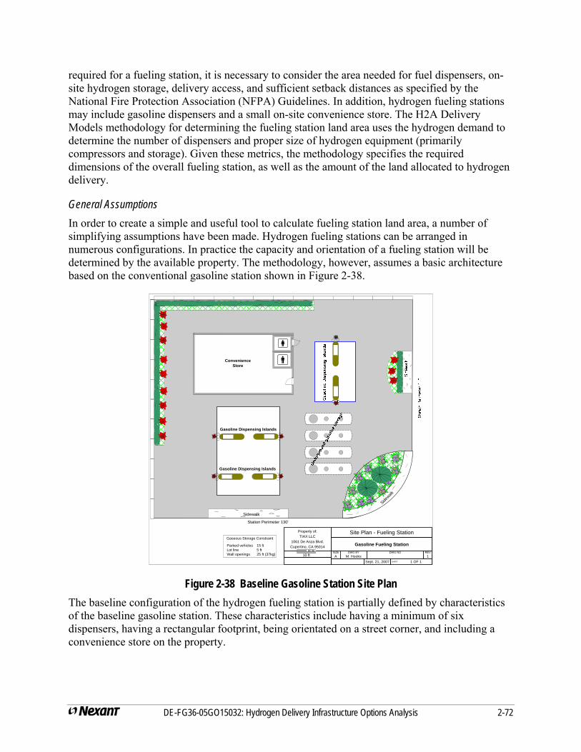
required for a fueling station, it is necessary to consider the area needed for fuel dispensers, on-site hydrogen storage, delivery access, and sufficient setback distances as specified by the National Fire Protection Association (NFPA) Guidelines. In addition, hydrogen fueling stations may include gasoline dispensers and a small on-site convenience store. The H2A Delivery Models methodology for determining the fueling station land area uses the hydrogen demand to determine the number of dispensers and proper size of hydrogen equipment (primarily compressors and storage). Given these metrics, the methodology specifies the required dimensions of the overall fueling station, as well as the amount of the land allocated to hydrogen delivery.
General Assumptions In order to create a simple and useful tool to calculate fueling station land area, a number of simplifying assumptions have been made. Hydrogen fueling stations can be arranged in numerous configurations. In practice the capacity and orientation of a fueling station will be determined by the available property. The methodology, however, assumes a basic architecture based on the conventional gasoline station shown in Figure 2-38.
Figure 2-38 Baseline Gasoline Station Site Plan
Property of:TIAX LLC
1061 De Anza Blvd.Cupertino, CA 95014
Site Plan - Fueling Station
Gasoline Fueling StationSIZE DWG BY DWG NO REVA M. Hooks 1
Sept. 21, 2007 SHEET 1 OF 1
10 ft
Gasoline Dispensing Islands
Convenience Store
Station Perimeter 130'
Sidewalk
Sidewalk
Gaseous Storage Constraint
Parked vehicles 15 ftLot line 5 ftWall openings 25 ft (37kg)
Gasoline Dispensing Islands
The baseline configuration of the hydrogen fueling station is partially defined by characteristics of the baseline gasoline station. These characteristics include having a minimum of six dispensers, having a rectangular footprint, being orientated on a street corner, and including a convenience store on the property.
DE-FG36-05GO15032: Hydrogen Delivery Infrastructure Options Analysis 2-72
The number of hydrogen dispensers at the fueling station is directly proportional to the hydrogen demand at the fueling station, This calculation is outlined in Section 2.3.2. Fueling stations that do not require six dispensers (an individual dispenser has two hoses and can fuel two vehicles simultaneously) to sufficiently meet the hydrogen demand, will have gasoline dispensers in addition to hydrogen dispensers. At these stations it is assumed that there are a total of six dispensers (hydrogen and gasoline). Additionally, it is assumed that if the hydrogen demand at the fueling station necessitates six or more dispensers, than the station will not have gasoline dispensers. The largest station considered consists of ten dispensers and is capable of dispensing 6,000 kg/day of hydrogen.
The land area allocated to hydrogen delivery is determined by the area required for the hydrogen equipment and the relative number of hydrogen and gasoline dispensers. The area occupied by the convenience store is not allocated to either gasoline or hydrogen delivery, as it will generally generate its own financial returns. If the land area required for the fueling station is in excess of the baseline gasoline station, the incremental station area is assigned to hydrogen. The baseline area (excluding the convenience store) is divided between hydrogen and gasoline delivery based on the proportion of dispensers that distribute each fuel. If the fueling station only contains hydrogen dispensers, all the land area except the convenience store will be allocated to hydrogen delivery.
Primary Variables A few primary variables determine the land area required for a hydrogen fueling station.
Daily Average Fuel Demand
− The daily average fuel demand is used to calculate the required number of dispensers and storage capacity. (These calculations are detailed in Sections 2.3.1 and 2.3.2 in this report).
− Average fuel demand is specified by the user in the Models setting the size of the refueling station.
Setback Distances
− Setback distances in this analysis are specified by the NFPA and apply to the location of hydrogen storage in relation to a variety of exposures.
− Setback distances are entered into the model as default values.
Delivery Method
− The options for delivery are: gaseous tube trailers, gaseous pipeline delivery, or liquid truck delivery. Each option has unique space requirements.
− The delivery method is specified by the user in the Models.
Setback Distances A major factor in determining the overall land area required for hydrogen fueling stations is the required setback distances from hydrogen storage. These distances are specified by the NFPA (Section 55, Chapter 10). The NFPA setback distances only dictate the relative location of
DE-FG36-05GO15032: Hydrogen Delivery Infrastructure Options Analysis 2-73
hydrogen storage and do not make any specifications as to the location of other hydrogen equipment or dispensers.
The regulations governing fueling stations are presently under review. Following this review, updated regulations may be released within the next two years. These changes will be released in NFPA 2. The updated regulations may change the basic assumptions and default values used in the H2A Delivery Models. It is unclear at this point how much effect the new regulations will have on the overall land area of the fueling station. Given new regulations, it is also unclear whether the fueling station area requirements will be able to be calculated simply by modifying input parameters. A thorough review of the new NFPA codes will be required upon their release.
It is also important to note that local authorities (generally fire departments) have final jurisdiction over setback distances. This authority allows local officials to make educated adjustments to the NFPA requirements. For example, it is possible for engineered systems (such as fire retardant walls) to be used in order to reduce the setbacks distances specified in NFPA 55 in situations where standard compliance with the standard regulations is challenging or impossible. The H2A Delivery Models do not take advantage of any engineered systems and uses all of the setback distances specified by NFPA 55. Specific setback distances can be found in Table 2-24.
Setback distances specify the distance required between hydrogen storage and specific points on the property, such as wall openings or lot lines. The area between these two points does not have to be vacant. For example, hydrogen storage can be next to the convenience store provided that the walls are sufficiently sprinkled and non-combustible, and that there are no wall openings within the setback distance specified by NFPA. In fact, the H2A Delivery Models now estimate the land area of the fueling station situating storage as close to the convenience store as possible while still maintaining the appropriate distance from wall openings (all doors are assumed to be on the opposite side of the structure). In addition, the other hydrogen components, such as vaporizers and compressors, can be situated within the setback distances surrounding the hydrogen storage. It is unnecessary to provide greater setbacks around those components. This is particularly evident as stations that are supplied with liquid hydrogen, as the vaporizer – a very large component, can be located within the setback around the liquid hydrogen tank.
The NFPA guidelines specify setbacks from flammable liquid storage (i.e. gasoline storage) and the associated components (vents and fills). These setback distances are also specified in Table 2-24. These setback distances were not explicitly included in the H2A Delivery Models given the assumption that they can more easily be located on the site outside the required setback distances.
Based on discussions with representatives from Air Products and Chemicals, there are no specific restrictions regarding the placement of hydrogen dispensers or regarding the relative placement of hydrogen and gasoline dispensers.
Relevant assumptions used to calculate the overall land area required for hydrogen delivery can be found below in Table 2-24.
DE-FG36-05GO15032: Hydrogen Delivery Infrastructure Options Analysis 2-74
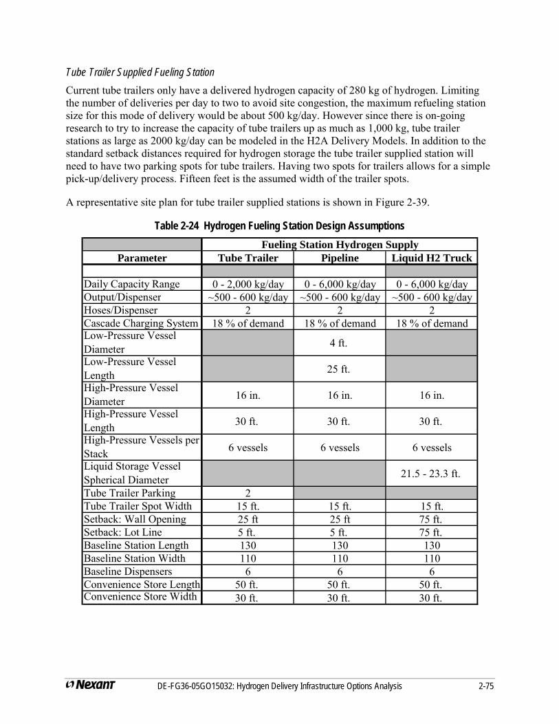
Tube Trailer Supplied Fueling Station Current tube trailers only have a delivered hydrogen capacity of 280 kg of hydrogen. Limiting the number of deliveries per day to two to avoid site congestion, the maximum refueling station size for this mode of delivery would be about 500 kg/day. However since there is on-going research to try to increase the capacity of tube trailers up as much as 1,000 kg, tube trailer stations as large as 2000 kg/day can be modeled in the H2A Delivery Models. In addition to the standard setback distances required for hydrogen storage the tube trailer supplied station will need to have two parking spots for tube trailers. Having two spots for trailers allows for a simple pick-up/delivery process. Fifteen feet is the assumed width of the trailer spots.
A representative site plan for tube trailer supplied stations is shown in Figure 2-39.
Table 2-24 Hydrogen Fueling Station Design Assumptions Fueling Station Hydrogen Supply
Parameter Tube Trailer Pipeline Liquid H2 Truck
Daily Capacity Range 0 - 2,000 kg/day 0 - 6,000 kg/day 0 - 6,000 kg/dayOutput/Dispenser ~500 - 600 kg/day ~500 - 600 kg/day ~500 - 600 kg/dayHoses/Dispenser 2 2 2Cascade Charging System 18 % of demand 18 % of demand 18 % of demandLow-Pressure Vessel Diameter 4 ft.
Low-Pressure Vessel Length 25 ft.
High-Pressure Vessel Diameter 16 in. 16 in. 16 in.
High-Pressure Vessel Length 30 ft. 30 ft. 30 ft.
High-Pressure Vessels per Stack 6 vessels 6 vessels 6 vessels
Liquid Storage Vessel Spherical Diameter 21.5 - 23.3 ft.
Tube Trailer Parking 2Tube Trailer Spot Width 15 ft. 15 ft. 15 ft.Setback: Wall Opening 25 ft 25 ft 75 ft. Setback: Lot Line 5 ft. 5 ft. 75 ft. Baseline Station Length 130 130 130Baseline Station Width 110 110 110Baseline Dispensers 6 6 6Convenience Store Length 50 ft. 50 ft. 50 ft. Convenience Store Width 30 ft. 30 ft. 30 ft.
DE-FG36-05GO15032: Hydrogen Delivery Infrastructure Options Analysis 2-75
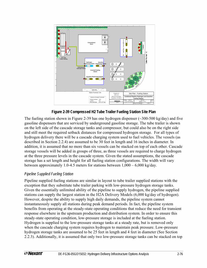
Figure 2-39 Compressed H2 Tube Trailer Fueling Station Site Plan
Property of:TIAX LLC
1061 De Anza Blvd.Cupertino, CA 95014
Site Plan - Fueling Station
Combined Pipeline Hydrogen and Gasoline Fueling Station
SIZE DWG BY DWG NO REV
A Erin Kassoy D0035 – P-L1 0Aug. 29, 2005 SHEET 1 OF 1
10 ft
Hydrogen Dispensing Island
Covered Fueling Island
Gasoline Dispensing Islands
Station Perimeter 150'
Sidewalk
Underground Hydrogen Piping
Sidewalk
Gaseous Storage Constraint
Parked vehicles 15 ftLot line 5 ftWall openings 25 ft (>37 kg)
cH2 Tube Trailer Parking
Gasoline Dispensing Island
Convenience Store
The fueling station shown in Figure 2-39 has one hydrogen dispenser (~300-500 kg/day) and five gasoline dispensers that are serviced by underground gasoline storage. The tube trailer is shown on the left side of the cascade storage tanks and compressor, but could also be on the right side and still meet the required setback distances for compressed hydrogen storage. For all types of hydrogen delivery there will be a cascade charging system used to fuel vehicles. The vessels (as described in Section 2.2.4) are assumed to be 30 feet in length and 16 inches in diameter. In addition, it is assumed that no more than six vessels can be stacked on top of each other. Cascade storage vessels will be added in groups of three, as three vessels are required to charge hydrogen at the three pressure levels in the cascade system. Given the stated assumptions, the cascade storage has a set length and height for all fueling station configurations. The width will vary between approximately 1.0-4.5 meters for stations between 1,000 – 6,000 kg/day.
Pipeline Supplied Fueling Station Pipeline supplied fueling stations are similar in layout to tube trailer supplied stations with the exception that they substitute tube trailer parking with low-pressure hydrogen storage tanks. Given the essentially unlimited ability of the pipeline to supply hydrogen, the pipeline supplied stations can supply the largest station in the H2A Delivery Models (6,000 kg/day of hydrogen). However, despite the ability to supply high daily demands, the pipeline system cannot instantaneously supply all stations during peak demand periods. In fact, the pipeline system benefits from operating at the steady-state operating conditions that reduce the need for transient response elsewhere in the upstream production and distribution system. In order to ensure this steady-state operating condition, low-pressure storage is included at the fueling station. Hydrogen is supplied to the low-pressure storage tanks at a steady rate, but is removed only when the cascade charging system requires hydrogen to maintain peak pressure. Low-pressure hydrogen storage tanks are assumed to be 25 feet in length and 4 feet in diameter (See Section 2.2.3). Additionally, it is assumed that only two low-pressure storage tanks can be stacked on top
DE-FG36-05GO15032: Hydrogen Delivery Infrastructure Options Analysis 2-76
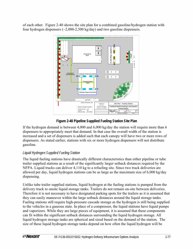
of each other. Figure 2-40 shows the site plan for a combined gasoline/hydrogen station with four hydrogen dispensers (~2,000-2,500 kg/day) and two gasoline dispensers.
Property of:TIAX LLC
1061 De Anza Blvd.Cupertino, CA 95014
Site Plan - Fueling Station
Combined Pipeline Hydrogen and Gasoline Fueling Station
SIZE DWG BY DWG NO REV
A Erin Kassoy D0035 – P-L1 3Aug. 29, 2005 SHEET 1 OF 1
10 ft
Hydrogen Dispensing Islands
Station Perimeter 130'
Sidewalk
Underground Hydrogen Piping
Sidewalk
Gaseous Storage Constraint
Parked vehicles 15 ftLot line 5 ftWall openings 25 ft (37kg)
Covered Fueling Island
Hydrogen Dispensing Islands
Compressor
Convenience Store
Figure 2-40 Pipeline Supplied Fueling Station Site Plan If the hydrogen demand is between 4,000 and 6,000 kg/day the station will require more than 6 dispensers to appropriately meet that demand. In that case the overall width of the station is increased and a set of dispensers is added such that each canopy will have two or more rows of dispensers. As stated earlier, stations with six or more hydrogen dispensers will not distribute gasoline.
Liquid Hydrogen Supplied Fueling Station The liquid fueling stations have drastically different characteristics than either pipeline or tube trailer supplied stations as a result of the significantly larger setback distances required by the NFPA. Liquid trucks can deliver 4,110 kg to a refueling site. Since two truck deliveries are allowed per day, liquid hydrogen stations can be as large as the maximum size of 6,000 kg/day dispensing.
Unlike tube trailer supplied stations, liquid hydrogen at the fueling stations is pumped from the delivery truck to onsite liquid storage tanks. Trailers do not remain on-site between deliveries. Therefore it is not necessary to have designated parking spots for the trailers as it is assumed that they can easily maneuver within the large setback distances around the liquid storage tanks. Fueling stations still require high-pressure cascade storage as the hydrogen is still being supplied to the vehicles in a gaseous state. In place of a compressor, the liquid stations have liquid pumps and vaporizers. While they are large pieces of equipment, it is assumed that these components can fit within the significant setback distances surrounding the liquid hydrogen storage. All liquid hydrogen storage tanks are spherical and sized based on the demand of the station. The size of these liquid hydrogen storage tanks depend on how often the liquid hydrogen will be
DE-FG36-05GO15032: Hydrogen Delivery Infrastructure Options Analysis 2-77
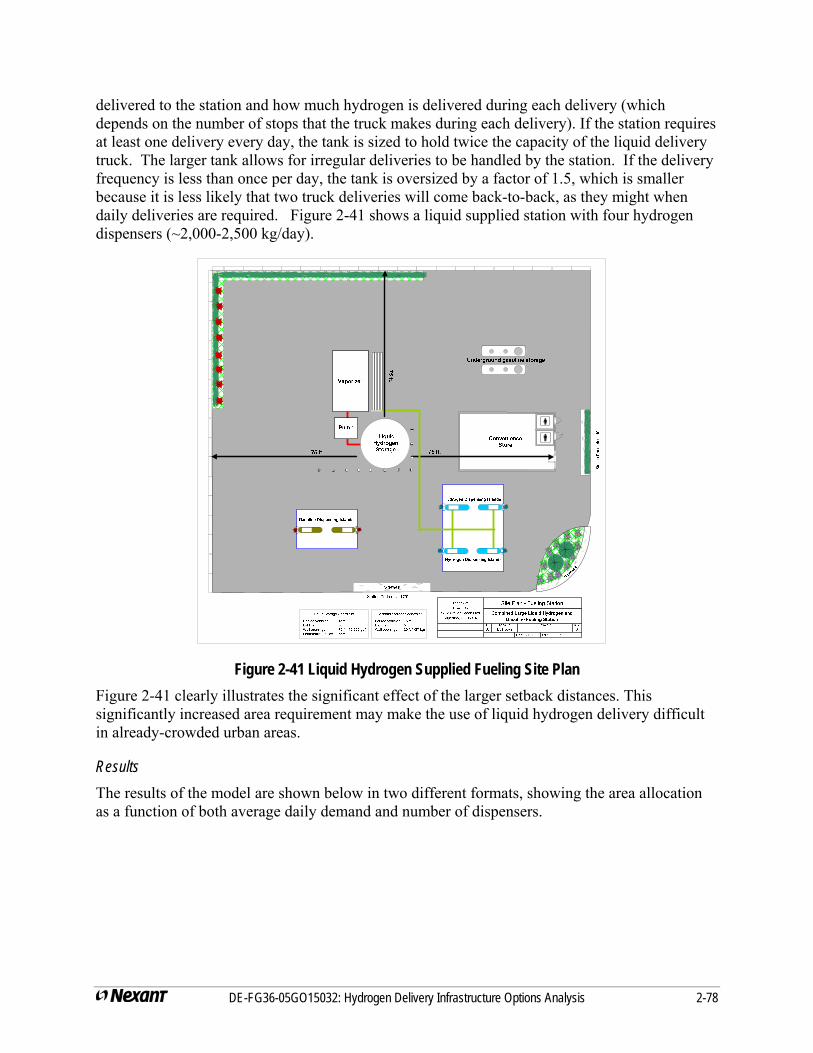
delivered to the station and how much hydrogen is delivered during each delivery (which depends on the number of stops that the truck makes during each delivery). If the station requires at least one delivery every day, the tank is sized to hold twice the capacity of the liquid delivery truck. The larger tank allows for irregular deliveries to be handled by the station. If the delivery frequency is less than once per day, the tank is oversized by a factor of 1.5, which is smaller because it is less likely that two truck deliveries will come back-to-back, as they might when daily deliveries are required. Figure 2-41 shows a liquid supplied station with four hydrogen dispensers (~2,000-2,500 kg/day).
Figure 2-41 Liquid Hydrogen Supplied Fueling Site Plan Figure 2-41 clearly illustrates the significant effect of the larger setback distances. This significantly increased area requirement may make the use of liquid hydrogen delivery difficult in already-crowded urban areas.
Results The results of the model are shown below in two different formats, showing the area allocation as a function of both average daily demand and number of dispensers.
DE-FG36-05GO15032: Hydrogen Delivery Infrastructure Options Analysis 2-78
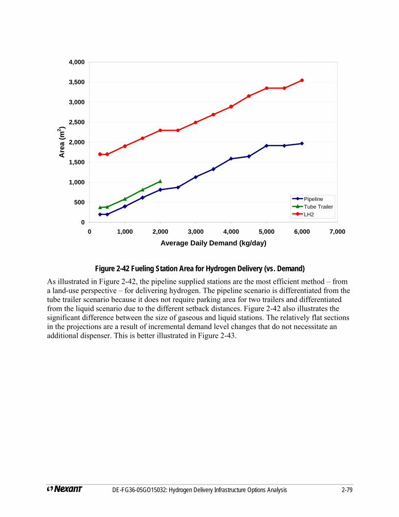
0
500
1,000
1,500
2,000
2,500
3,000
3,500
4,000
0 1,000 2,000 3,000 4,000 5,000 6,000 7,000
Average Daily Demand (kg/day)
Are
a (m
2 )
PipelineTube TrailerLH2
Figure 2-42 Fueling Station Area for Hydrogen Delivery (vs. Demand) As illustrated in Figure 2-42, the pipeline supplied stations are the most efficient method – from a land-use perspective – for delivering hydrogen. The pipeline scenario is differentiated from the tube trailer scenario because it does not require parking area for two trailers and differentiated from the liquid scenario due to the different setback distances. Figure 2-42 also illustrates the significant difference between the size of gaseous and liquid stations. The relatively flat sections in the projections are a result of incremental demand level changes that do not necessitate an additional dispenser. This is better illustrated in Figure 2-43.
DE-FG36-05GO15032: Hydrogen Delivery Infrastructure Options Analysis 2-79
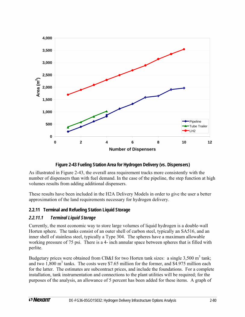
DE-FG36-05GO15032: Hydrogen Delivery Infrastructure Options Analysis 2-80
0
500
1,000
1,500
2,000
2,500
3,000
3,500
4,000
0 2 4 6 8 10
Number of Dispensers
Are
a (m
2 )
12
PipelineTube TrailerLH2
Figure 2-43 Fueling Station Area for Hydrogen Delivery (vs. Dispensers) As illustrated in Figure 2-43, the overall area requirement tracks more consistently with the number of dispensers than with fuel demand. In the case of the pipeline, the step function at high volumes results from adding additional dispensers.
These results have been included in the H2A Delivery Models in order to give the user a better approximation of the land requirements necessary for hydrogen delivery.
2.2.11 Terminal and Refueling Station Liquid Storage 2.2.11.1 Terminal Liquid Storage Currently, the most economic way to store large volumes of liquid hydrogen is a double-wall Horten sphere. The tanks consist of an outer shell of carbon steel, typically an SA516, and an inner shell of stainless steel, typically a Type 304. The spheres have a maximum allowable working pressure of 75 psi. There is a 4- inch annular space between spheres that is filled with perlite.
Budgetary prices were obtained from CB&I for two Horten tank sizes: a single 3,500 m3 tank; and two 1,800 m3 tanks. The costs were $7.65 million for the former, and $4.975 million each for the latter. The estimates are subcontract prices, and include the foundations. For a complete installation, tank instrumentation and connections to the plant utilities will be required; for the purposes of the analysis, an allowance of 5 percent has been added for these items. A graph of
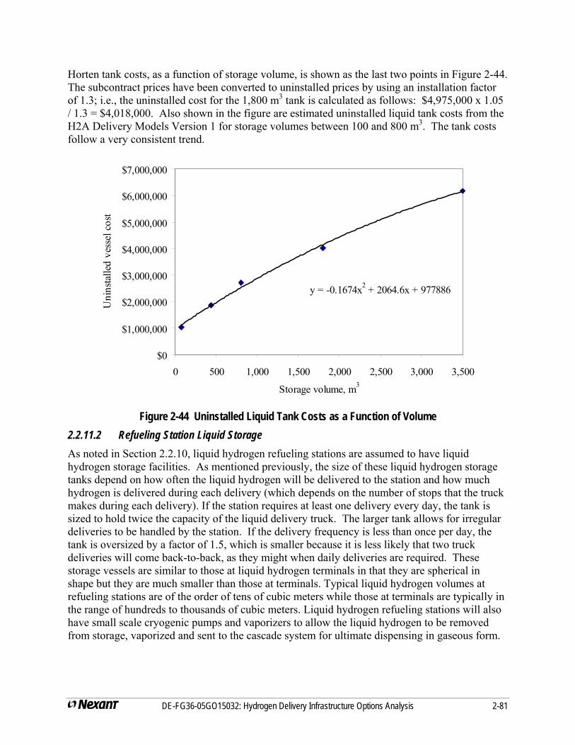
Horten tank costs, as a function of storage volume, is shown as the last two points in Figure 2-44. The subcontract prices have been converted to uninstalled prices by using an installation factor of 1.3; i.e., the uninstalled cost for the 1,800 m3 tank is calculated as follows: $4,975,000 x 1.05 / 1.3 = $4,018,000. Also shown in the figure are estimated uninstalled liquid tank costs from the H2A Delivery Models Version 1 for storage volumes between 100 and 800 m3. The tank costs follow a very consistent trend.
y = -0.1674x2 + 2064.6x + 977886
$0
$1,000,000
$2,000,000
$3,000,000
$4,000,000
$5,000,000
$6,000,000
$7,000,000
0 500 1,000 1,500 2,000 2,500 3,000 3,500
Storage volume, m3
Uni
nsta
lled
vess
el c
ost
Figure 2-44 Uninstalled Liquid Tank Costs as a Function of Volume 2.2.11.2 Refueling Station Liquid Storage As noted in Section 2.2.10, liquid hydrogen refueling stations are assumed to have liquid hydrogen storage facilities. As mentioned previously, the size of these liquid hydrogen storage tanks depend on how often the liquid hydrogen will be delivered to the station and how much hydrogen is delivered during each delivery (which depends on the number of stops that the truck makes during each delivery). If the station requires at least one delivery every day, the tank is sized to hold twice the capacity of the liquid delivery truck. The larger tank allows for irregular deliveries to be handled by the station. If the delivery frequency is less than once per day, the tank is oversized by a factor of 1.5, which is smaller because it is less likely that two truck deliveries will come back-to-back, as they might when daily deliveries are required. These storage vessels are similar to those at liquid hydrogen terminals in that they are spherical in shape but they are much smaller than those at terminals. Typical liquid hydrogen volumes at refueling stations are of the order of tens of cubic meters while those at terminals are typically in the range of hundreds to thousands of cubic meters. Liquid hydrogen refueling stations will also have small scale cryogenic pumps and vaporizers to allow the liquid hydrogen to be removed from storage, vaporized and sent to the cascade system for ultimate dispensing in gaseous form.
DE-FG36-05GO15032: Hydrogen Delivery Infrastructure Options Analysis 2-81
For liquid storage at refueling stations, a value for uninstalled cost of $70/kg of hydrogen stored is used in the H2A Delivery Models. This value comes from discussions with vendors when the H2A Delivery Models Version 1 was first generated. When an installation factor of 1.2 is applied, this value represents an installed cost of $84/kg.
2.2.12 Geologic Storage One of the options available in the H2A Delivery Models is the selection of gaseous geologic storage to meet the peak summer demand and to meet the total demand during the winter annually-scheduled shutdown of the hydrogen production plant. The summer demand peak is entered in the model as a percent of the average daily demand along with the duration. The default values are 10% above the average for 120 days (4 months). The winter plant outage default is 10 days. The geologic storage is sized to meet the larger storage need of these two situations.
H2A Delivery Models Version 2.0 is based on the use of salt caverns for underground storage of hydrogen. Other geologic storage technologies are not yet in the model. This technology was chosen for four reasons. First, there are two existing hydrogen salt caverns in the U.S. in Texas. We are not aware of any other types of geologic storage in use for hydrogen. Second, salt caverns are known for their capability to be cycled much more rapidly than other types of underground storage. The daily release from salt caverns can be as high as 11 percent of the working gas capacity (a 10 percent default value is used in the model) whereas 2 to 3 percent is typical for other underground storage options. As one of the objectives of geologic storage is to fully meet the hydrogen demand during times of production plant shutdown, the capacity of other geologic storage options would have to be 3 to 5 times greater than for a salt cavern. Third, the amount of base or cushion gas required in salt caverns appears to be lower than for the other options. Values as low as 20 percent of the working capacity have been reported, whereas requirements for other underground options appear to be in the 40 to 50 percent range. Thus the capital requirement for cushion gas in salt caverns is considerably less than for other options. Fourth, although the data are scattered and not always consistent, H2A Delivery Models developers were able to find more usable cost information for salt caverns than for other options. The initial phase of the Saltville natural gas storage facility in southwest Virginia served as the reference point for the costs in the model. These costs are in line with some cost information obtained from ConocoPhillips who are utilizing one of the two existing hydrogen geologic salt caverns in the U.S. located in Texas.
It is assumed that the geologic facility is located at or near to the hydrogen production facility. The delivery infrastructure costs would not be significantly affected as long as the geologic storage is located close to the production site, along the gaseous pipeline or near a city gate terminal in a mixed mode delivery pathway. If the pipeline delivery pathway has been selected, the cavern is filled by drawing from hydrogen at a pressure equal to the maximum pipeline pressure and discharges hydrogen at this same pressure. If the gaseous-hydrogen truck delivery pathway has been selected, the cavern withdraws hydrogen at a pressure equal to the hydrogen pressure at the gaseous terminal and ultimately discharges at approximately this same pressure. These pressures are consistent with the basic assumption that both the geologic storage facility and the gaseous-hydrogen terminal (if appropriate) are located at or adjacent to the hydrogen production facility.
DE-FG36-05GO15032: Hydrogen Delivery Infrastructure Options Analysis 2-82
Input to the geologic storage facility in the H2A Delivery Models includes the summer surge percentage (expressed as the percent above the annual average daily demand), the number of days that the surge continues, the number of days that the winter demand lasts, the number of days of scheduled production- plant outage, the maximum and minimum cavern pressures (i.e., full and with only the base or cushion gas), the hydrogen pressure from which the cavern is fed and the pressure to which the hydrogen is fed upon withdrawal from the cavern, the maximum allowable discharge rate, and the maximum allowable rate at which the cavern can be filled.
The H2A Delivery Models use the input parameters to determine the quantity of hydrogen that must be placed in geologic storage. This quantity is the greater of the quantity needed to meet the summer surge or the quantity needed to meet demand during the production-plant shutdown. In other words, the model determines this quantity under the assumption that the production-plant shutdown will be during the winter months of lowest demand. Another assumption in determining this quantity of hydrogen is that the amount of hydrogen consumed during the summer surge is equal to the difference between the amount of hydrogen actually consumed during the winter period (the lowest demand time of the year) and the amount that would be consumed if the annual-average daily demand were to exist over the same period. Based on the maximum and minimum pressures (i.e., full and empty except for cushion gas) the model determines the actual design capacity of the cavern.
The H2A Delivery Models then do an internal check to assure that the required hydrogen withdrawal rate is not greater than the input value. Should this occur, the model re-calculates the cavern volume so that this limitation is not exceeded.
Using the above calculated information along with user supplied values for numbers of compressors to be used, compression ratios, and compressor efficiencies, the H2A Delivery Models conduct several internal checks on hydrogen volumes and flow rates and estimate energy requirements for the compressors. The compressors are sized based on the greater of the following two pressure ratios: Maximum cavern pressure/inlet (fill) pressure or Outlet (discharge)/Minimum cavern pressure. Compressors are designed to handle one-half the total hydrogen throughput and an equally sized installed spare unit is also available for reliability purposes. In Version 2.0, the cavern must be completely filled, and then completely discharged, i.e., intermediate filling is not allowed.
Based on the physical parameters as input by the user and calculation as described above, the H2A Delivery Models then determines the capital and operating cost for the geologic storage facility. Many of the capital cost components are scaled from information available from the Saltville natural gas storage facility in southwest Virginia. These cost equations are presented below. Other costs, e.g., compressors, are calculated in a manner consistent with costs for equivalent equipment in other parts of the H2A Delivery Models.
Installed Cavern Cost = 3,738,563 * (cavern Nm3/19,000,000)0.7
Installed Miscellaneous Equipment Cost = 1,906,484 * (cavern Nm3/19,000,000)0.7
2.2.13 Oversize Transmission Pipeline as Storage As discussed in this report, in the standard pipeline delivery pathways modeled in the H2A Delivery Models, low pressure gas storage is used to handle the hourly demand variations at the
DE-FG36-05GO15032: Hydrogen Delivery Infrastructure Options Analysis 2-83
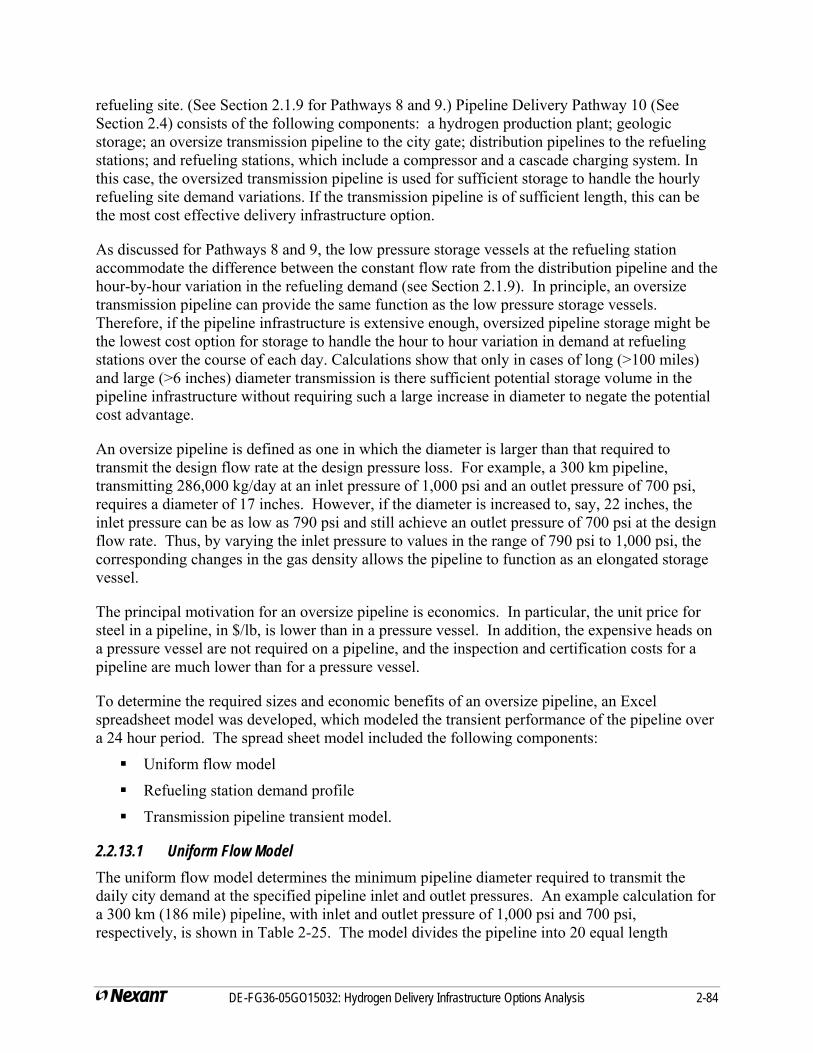
refueling site. (See Section 2.1.9 for Pathways 8 and 9.) Pipeline Delivery Pathway 10 (See Section 2.4) consists of the following components: a hydrogen production plant; geologic storage; an oversize transmission pipeline to the city gate; distribution pipelines to the refueling stations; and refueling stations, which include a compressor and a cascade charging system. In this case, the oversized transmission pipeline is used for sufficient storage to handle the hourly refueling site demand variations. If the transmission pipeline is of sufficient length, this can be the most cost effective delivery infrastructure option.
As discussed for Pathways 8 and 9, the low pressure storage vessels at the refueling station accommodate the difference between the constant flow rate from the distribution pipeline and the hour-by-hour variation in the refueling demand (see Section 2.1.9). In principle, an oversize transmission pipeline can provide the same function as the low pressure storage vessels. Therefore, if the pipeline infrastructure is extensive enough, oversized pipeline storage might be the lowest cost option for storage to handle the hour to hour variation in demand at refueling stations over the course of each day. Calculations show that only in cases of long (>100 miles) and large (>6 inches) diameter transmission is there sufficient potential storage volume in the pipeline infrastructure without requiring such a large increase in diameter to negate the potential cost advantage.
An oversize pipeline is defined as one in which the diameter is larger than that required to transmit the design flow rate at the design pressure loss. For example, a 300 km pipeline, transmitting 286,000 kg/day at an inlet pressure of 1,000 psi and an outlet pressure of 700 psi, requires a diameter of 17 inches. However, if the diameter is increased to, say, 22 inches, the inlet pressure can be as low as 790 psi and still achieve an outlet pressure of 700 psi at the design flow rate. Thus, by varying the inlet pressure to values in the range of 790 psi to 1,000 psi, the corresponding changes in the gas density allows the pipeline to function as an elongated storage vessel.
The principal motivation for an oversize pipeline is economics. In particular, the unit price for steel in a pipeline, in $/lb, is lower than in a pressure vessel. In addition, the expensive heads on a pressure vessel are not required on a pipeline, and the inspection and certification costs for a pipeline are much lower than for a pressure vessel.
To determine the required sizes and economic benefits of an oversize pipeline, an Excel spreadsheet model was developed, which modeled the transient performance of the pipeline over a 24 hour period. The spread sheet model included the following components:
Uniform flow model
Refueling station demand profile
Transmission pipeline transient model.
2.2.13.1 Uniform Flow Model The uniform flow model determines the minimum pipeline diameter required to transmit the daily city demand at the specified pipeline inlet and outlet pressures. An example calculation for a 300 km (186 mile) pipeline, with inlet and outlet pressure of 1,000 psi and 700 psi, respectively, is shown in Table 2-25. The model divides the pipeline into 20 equal length
DE-FG36-05GO15032: Hydrogen Delivery Infrastructure Options Analysis 2-84
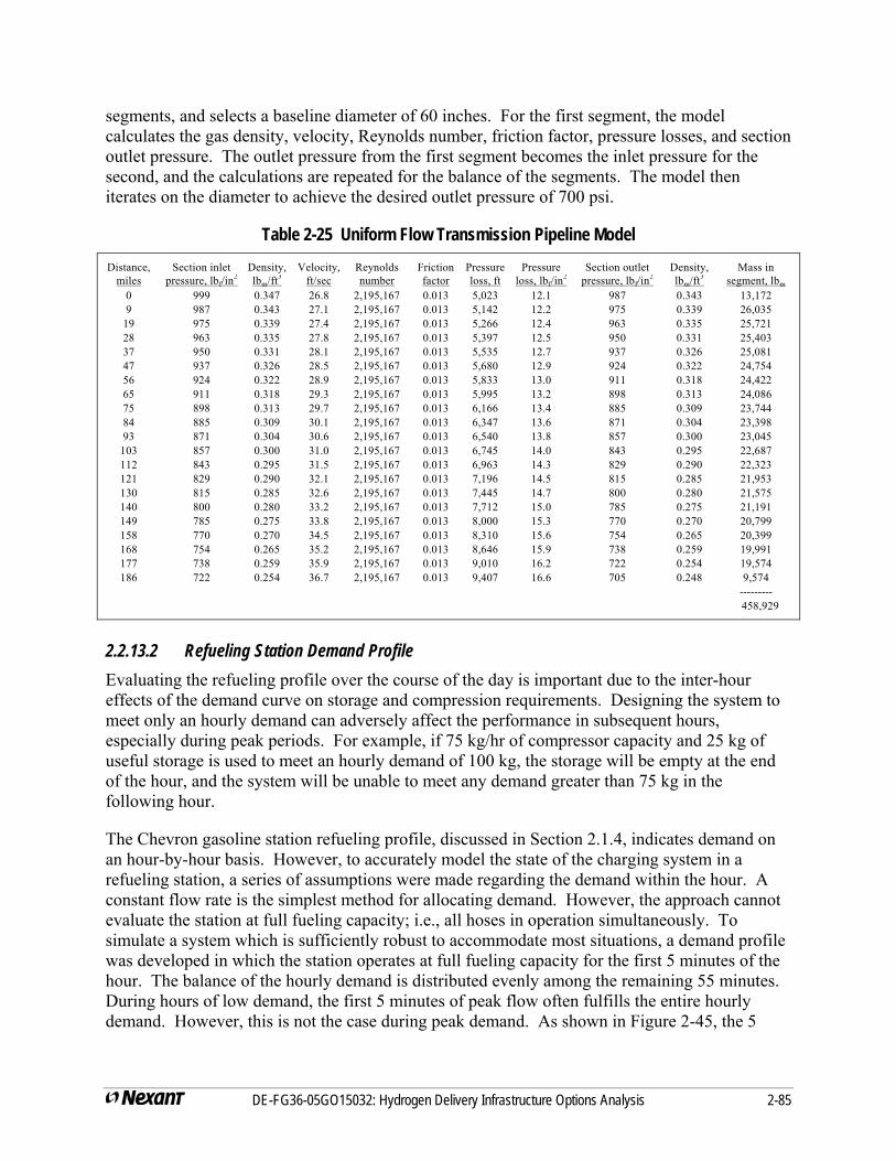
segments, and selects a baseline diameter of 60 inches. For the first segment, the model calculates the gas density, velocity, Reynolds number, friction factor, pressure losses, and section outlet pressure. The outlet pressure from the first segment becomes the inlet pressure for the second, and the calculations are repeated for the balance of the segments. The model then iterates on the diameter to achieve the desired outlet pressure of 700 psi.
Table 2-25 Uniform Flow Transmission Pipeline Model Distance, Section inlet Density, Velocity, Reynolds Friction Pressure Pressure Section outlet Density, Mass in
miles pressure, lbf/in2 lbm/ft3 ft/sec number factor loss, ft loss, lbf/in
2 pressure, lbf/in2 lbm/ft3 segment, lbm
0 999 0.347 26.8 2,195,167 0.013 5,023 12.1 987 0.343 13,1729 987 0.343 27.1 2,195,167 0.013 5,142 12.2 975 0.339 26,035
19 975 0.339 27.4 2,195,167 0.013 5,266 12.4 963 0.335 25,72128 963 0.335 27.8 2,195,167 0.013 5,397 12.5 950 0.331 25,40337 950 0.331 28.1 2,195,167 0.013 5,535 12.7 937 0.326 25,08147 937 0.326 28.5 2,195,167 0.013 5,680 12.9 924 0.322 24,75456 924 0.322 28.9 2,195,167 0.013 5,833 13.0 911 0.318 24,42265 911 0.318 29.3 2,195,167 0.013 5,995 13.2 898 0.313 24,08675 898 0.313 29.7 2,195,167 0.013 6,166 13.4 885 0.309 23,74484 885 0.309 30.1 2,195,167 0.013 6,347 13.6 871 0.304 23,39893 871 0.304 30.6 2,195,167 0.013 6,540 13.8 857 0.300 23,045
103 857 0.300 31.0 2,195,167 0.013 6,745 14.0 843 0.295 22,687112 843 0.295 31.5 2,195,167 0.013 6,963 14.3 829 0.290 22,323121 829 0.290 32.1 2,195,167 0.013 7,196 14.5 815 0.285 21,953130 815 0.285 32.6 2,195,167 0.013 7,445 14.7 800 0.280 21,575140 800 0.280 33.2 2,195,167 0.013 7,712 15.0 785 0.275 21,191149 785 0.275 33.8 2,195,167 0.013 8,000 15.3 770 0.270 20,799158 770 0.270 34.5 2,195,167 0.013 8,310 15.6 754 0.265 20,399168 754 0.265 35.2 2,195,167 0.013 8,646 15.9 738 0.259 19,991177 738 0.259 35.9 2,195,167 0.013 9,010 16.2 722 0.254 19,574186 722 0.254 36.7 2,195,167 0.013 9,407 16.6 705 0.248 9,574
---------458,929
2.2.13.2 Refueling Station Demand Profile Evaluating the refueling profile over the course of the day is important due to the inter-hour effects of the demand curve on storage and compression requirements. Designing the system to meet only an hourly demand can adversely affect the performance in subsequent hours, especially during peak periods. For example, if 75 kg/hr of compressor capacity and 25 kg of useful storage is used to meet an hourly demand of 100 kg, the storage will be empty at the end of the hour, and the system will be unable to meet any demand greater than 75 kg in the following hour.
The Chevron gasoline station refueling profile, discussed in Section 2.1.4, indicates demand on an hour-by-hour basis. However, to accurately model the state of the charging system in a refueling station, a series of assumptions were made regarding the demand within the hour. A constant flow rate is the simplest method for allocating demand. However, the approach cannot evaluate the station at full fueling capacity; i.e., all hoses in operation simultaneously. To simulate a system which is sufficiently robust to accommodate most situations, a demand profile was developed in which the station operates at full fueling capacity for the first 5 minutes of the hour. The balance of the hourly demand is distributed evenly among the remaining 55 minutes. During hours of low demand, the first 5 minutes of peak flow often fulfills the entire hourly demand. However, this is not the case during peak demand. As shown in Figure 2-45, the 5
DE-FG36-05GO15032: Hydrogen Delivery Infrastructure Options Analysis 2-85
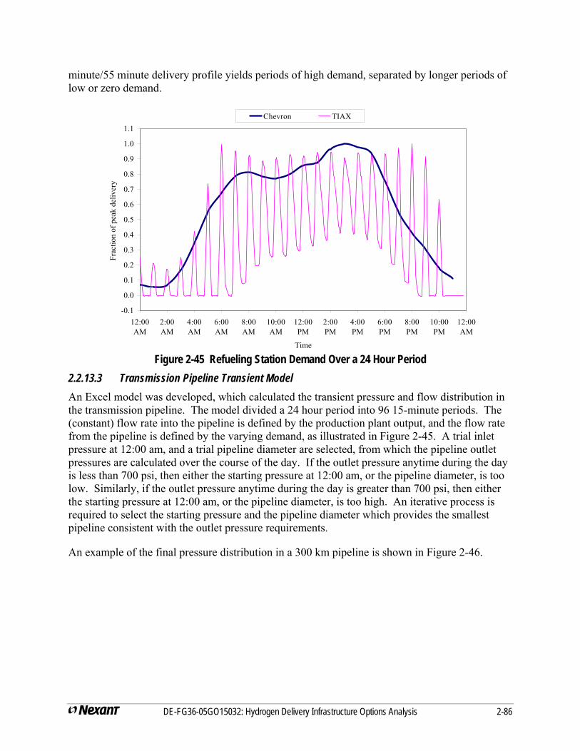
minute/55 minute delivery profile yields periods of high demand, separated by longer periods of low or zero demand.
-0.1
0.0
0.1
0.2
0.3
0.4
0.5
0.6
0.7
0.8
0.9
1.0
1.1
12:00AM
2:00AM
4:00AM
6:00AM
8:00AM
10:00AM
12:00PM
2:00PM
4:00PM
6:00PM
8:00PM
10:00PM
12:00AM
Time
Frac
tion
of p
eak
deliv
ery
Chevron TIAX
Figure 2-45 Refueling Station Demand Over a 24 Hour Period
2.2.13.3 Transmission Pipeline Transient Model An Excel model was developed, which calculated the transient pressure and flow distribution in the transmission pipeline. The model divided a 24 hour period into 96 15-minute periods. The (constant) flow rate into the pipeline is defined by the production plant output, and the flow rate from the pipeline is defined by the varying demand, as illustrated in Figure 2-45. A trial inlet pressure at 12:00 am, and a trial pipeline diameter are selected, from which the pipeline outlet pressures are calculated over the course of the day. If the outlet pressure anytime during the day is less than 700 psi, then either the starting pressure at 12:00 am, or the pipeline diameter, is too low. Similarly, if the outlet pressure anytime during the day is greater than 700 psi, then either the starting pressure at 12:00 am, or the pipeline diameter, is too high. An iterative process is required to select the starting pressure and the pipeline diameter which provides the smallest pipeline consistent with the outlet pressure requirements.
An example of the final pressure distribution in a 300 km pipeline is shown in Figure 2-46.
DE-FG36-05GO15032: Hydrogen Delivery Infrastructure Options Analysis 2-86
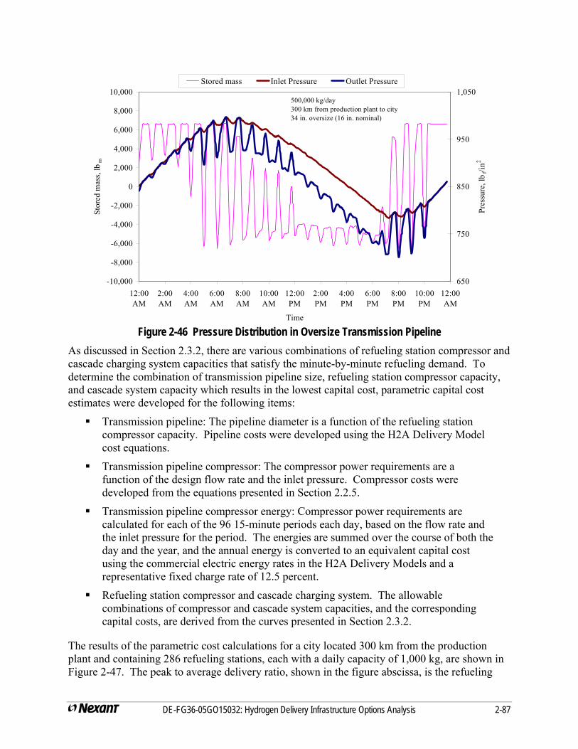
-10,000
-8,000
-6,000
-4,000
-2,000
0
2,000
4,000
6,000
8,000
10,000
12:00AM
2:00AM
4:00AM
6:00AM
8:00AM
10:00AM
12:00PM
2:00PM
4:00PM
6:00PM
8:00PM
10:00PM
12:00AM
Time
Stor
ed m
ass,
lbm
650
750
850
950
1,050
Pres
sure
, lb f
/in2
Stored mass Inlet Pressure Outlet Pressure
500,000 kg/day300 km from production plant to city34 in. oversize (16 in. nominal)
Figure 2-46 Pressure Distribution in Oversize Transmission Pipeline
As discussed in Section 2.3.2, there are various combinations of refueling station compressor and cascade charging system capacities that satisfy the minute-by-minute refueling demand. To determine the combination of transmission pipeline size, refueling station compressor capacity, and cascade system capacity which results in the lowest capital cost, parametric capital cost estimates were developed for the following items:
Transmission pipeline: The pipeline diameter is a function of the refueling station compressor capacity. Pipeline costs were developed using the H2A Delivery Model cost equations.
Transmission pipeline compressor: The compressor power requirements are a function of the design flow rate and the inlet pressure. Compressor costs were developed from the equations presented in Section 2.2.5.
Transmission pipeline compressor energy: Compressor power requirements are calculated for each of the 96 15-minute periods each day, based on the flow rate and the inlet pressure for the period. The energies are summed over the course of both the day and the year, and the annual energy is converted to an equivalent capital cost using the commercial electric energy rates in the H2A Delivery Models and a representative fixed charge rate of 12.5 percent.
Refueling station compressor and cascade charging system. The allowable combinations of compressor and cascade system capacities, and the corresponding capital costs, are derived from the curves presented in Section 2.3.2.
The results of the parametric cost calculations for a city located 300 km from the production plant and containing 286 refueling stations, each with a daily capacity of 1,000 kg, are shown in Figure 2-47. The peak to average delivery ratio, shown in the figure abscissa, is the refueling
DE-FG36-05GO15032: Hydrogen Delivery Infrastructure Options Analysis 2-87

DE-FG36-05GO15032: Hydrogen Delivery Infrastructure Options Analysis 2-88
station compressor capacity divided by the average hydrogen dispensed in a 24 hour period. The delivery + refueling station costs, shown in the figure ordinate, is the sum of the following: transmission pipeline cost; pipeline compressor cost; equivalent capital cost for the energy to operate the pipeline compressor; refueling station compressor cost; and cascade charging system cost.
$400,000
$420,000
$440,000
$460,000
$480,000
$500,000
$520,000
$540,000
1.5 2.0 2.5 3.0Peak to average delivery ratio
Del
iver
y +
fore
cour
t cos
t, $1
000
3.5
Figure 2-47 Pathway 3 Delivery System Optimization
For the combination of design parameters; the optimum delivery pathway consists of the following items:
22 inch diameter transmission pipeline
4,250 kWe pipeline compressor
83 kg/hr refueling station compressor
198 kg cascade charging system.
2.2.14 Hydrogen Losses Each component within the delivery infrastructure may include hydrogen losses. For example, liquid hydrogen stored in a well-insulated storage vessel may boil-off, and be lost through a pressure relief valve. These losses become important variables when calculating the hydrogen required by each component in a pathway, and for calculating the design flow rate for each component.
The Nexant team consulted with a variety of industry suppliers to determine the anticipated losses for a range of components. The values shown in Table 2-26 are those used in the H2A Delivery Models Version 2.
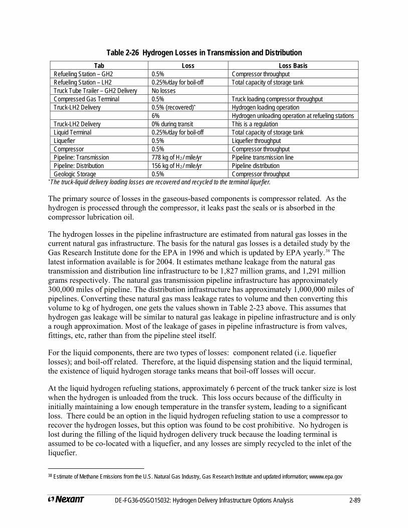
DE-FG36-05GO15032: Hydrogen Delivery Infrastructure Options Analysis 2-89
Table 2-26 Hydrogen Losses in Transmission and Distribution Tab Loss Loss Basis
Refueling Station – GH2 0.5% Compressor throughput Refueling Station – LH2 0.25%/day for boil-off Total capacity of storage tank Truck Tube Trailer – GH2 Delivery No losses Compressed Gas Terminal 0.5% Truck loading compressor throughput Truck-LH2 Delivery 0.5% (recovered)* Hydrogen loading operation 6% Hydrogen unloading operation at refueling stations Truck-LH2 Delivery 0% during transit This is a regulation Liquid Terminal 0.25%/day for boil-off Total capacity of storage tank Liquefier 0.5% Liquefier throughput Compressor 0.5% Compressor throughput Pipeline: Transmission 778 kg of H2/ mile/yr Pipeline transmission line Pipeline: Distribution 156 kg of H2/ mile/yr Pipeline distribution Geologic Storage 0.5% Compressor throughput
* The truck-liquid delivery loading losses are recovered and recycled to the terminal liquefier.
The primary source of losses in the gaseous-based components is compressor related. As the hydrogen is processed through the compressor, it leaks past the seals or is absorbed in the compressor lubrication oil.
The hydrogen losses in the pipeline infrastructure are estimated from natural gas losses in the current natural gas infrastructure. The basis for the natural gas losses is a detailed study by the Gas Research Institute done for the EPA in 1996 and which is updated by EPA yearly.38 The latest information available is for 2004. It estimates methane leakage from the natural gas transmission and distribution line infrastructure to be 1,827 million grams, and 1,291 million grams respectively. The natural gas transmission pipeline infrastructure has approximately 300,000 miles of pipeline. The distribution infrastructure has approximately 1,000,000 miles of pipelines. Converting these natural gas mass leakage rates to volume and then converting this volume to kg of hydrogen, one gets the values shown in Table 2-23 above. This assumes that hydrogen gas leakage will be similar to natural gas leakage in pipeline infrastructure and is only a rough approximation. Most of the leakage of gases in pipeline infrastructure is from valves, fittings, etc, rather than from the pipeline steel itself.
For the liquid components, there are two types of losses: component related (i.e. liquefier losses); and boil-off related. Therefore, at the liquid dispensing station and the liquid terminal, the existence of liquid hydrogen storage tanks means that boil-off losses will occur.
At the liquid hydrogen refueling stations, approximately 6 percent of the truck tanker size is lost when the hydrogen is unloaded from the truck. This loss occurs because of the difficulty in initially maintaining a low enough temperature in the transfer system, leading to a significant loss. There could be an option in the liquid hydrogen refueling station to use a compressor to recover the hydrogen losses, but this option was found to be cost prohibitive. No hydrogen is lost during the filling of the liquid hydrogen delivery truck because the loading terminal is assumed to be co-located with a liquefier, and any losses are simply recycled to the inlet of the liquefier.
38 Estimate of Methane Emissions from the U.S. Natural Gas Industry, Gas Research Institute and updated information; wwww.epa.gov
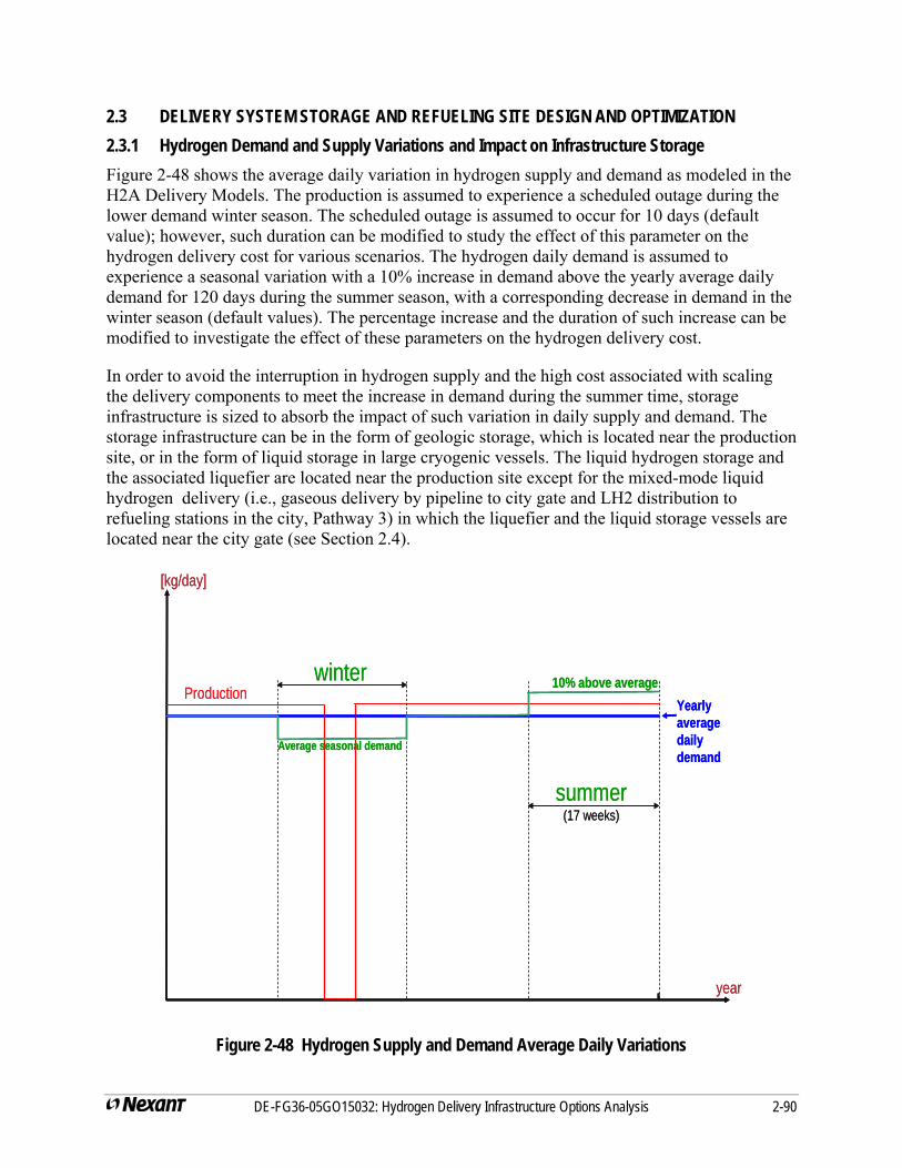
2.3 DELIVERY SYSTEM STORAGE AND REFUELING SITE DESIGN AND OPTIMIZATION 2.3.1 Hydrogen Demand and Supply Variations and Impact on Infrastructure Storage Figure 2-48 shows the average daily variation in hydrogen supply and demand as modeled in the H2A Delivery Models. The production is assumed to experience a scheduled outage during the lower demand winter season. The scheduled outage is assumed to occur for 10 days (default value); however, such duration can be modified to study the effect of this parameter on the hydrogen delivery cost for various scenarios. The hydrogen daily demand is assumed to experience a seasonal variation with a 10% increase in demand above the yearly average daily demand for 120 days during the summer season, with a corresponding decrease in demand in the winter season (default values). The percentage increase and the duration of such increase can be modified to investigate the effect of these parameters on the hydrogen delivery cost.
In order to avoid the interruption in hydrogen supply and the high cost associated with scaling the delivery components to meet the increase in demand during the summer time, storage infrastructure is sized to absorb the impact of such variation in daily supply and demand. The storage infrastructure can be in the form of geologic storage, which is located near the production site, or in the form of liquid storage in large cryogenic vessels. The liquid hydrogen storage and the associated liquefier are located near the production site except for the mixed-mode liquid hydrogen delivery (i.e., gaseous delivery by pipeline to city gate and LH2 distribution to refueling stations in the city, Pathway 3) in which the liquefier and the liquid storage vessels are located near the city gate (see Section 2.4).
winter
summer(17 weeks)
10% above averageProduction
Yearly average dailydemand
Average seasonal demand
[kg/day]
year
winter
summer(17 weeks)
10% above averageProduction
Yearly average dailydemand
Average seasonal demand
[kg/day]
year
Figure 2-48 Hydrogen Supply and Demand Average Daily Variations
DE-FG36-05GO15032: Hydrogen Delivery Infrastructure Options Analysis 2-90
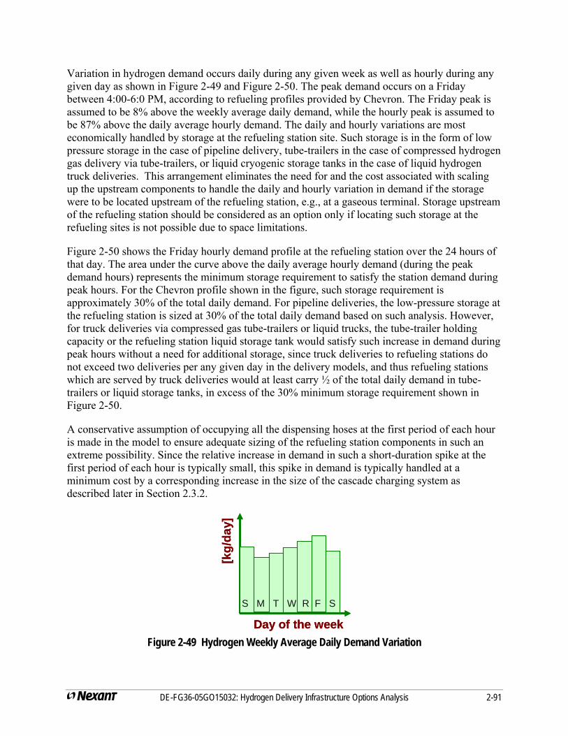
DE-FG36-05GO15032: Hydrogen Delivery Infrastructure Options Analysis 2-91
Variation in hydrogen demand occurs daily during any given week as well as hourly during any given day as shown in Figure 2-49 and Figure 2-50. The peak demand occurs on a Friday between 4:00-6:0 PM, according to refueling profiles provided by Chevron. The Friday peak is assumed to be 8% above the weekly average daily demand, while the hourly peak is assumed to be 87% above the daily average hourly demand. The daily and hourly variations are most economically handled by storage at the refueling station site. Such storage is in the form of low pressure storage in the case of pipeline delivery, tube-trailers in the case of compressed hydrogen gas delivery via tube-trailers, or liquid cryogenic storage tanks in the case of liquid hydrogen truck deliveries. This arrangement eliminates the need for and the cost associated with scaling up the upstream components to handle the daily and hourly variation in demand if the storage were to be located upstream of the refueling station, e.g., at a gaseous terminal. Storage upstream of the refueling station should be considered as an option only if locating such storage at the refueling sites is not possible due to space limitations.
Figure 2-50 shows the Friday hourly demand profile at the refueling station over the 24 hours of that day. The area under the curve above the daily average hourly demand (during the peak demand hours) represents the minimum storage requirement to satisfy the station demand during peak hours. For the Chevron profile shown in the figure, such storage requirement is approximately 30% of the total daily demand. For pipeline deliveries, the low-pressure storage at the refueling station is sized at 30% of the total daily demand based on such analysis. However, for truck deliveries via compressed gas tube-trailers or liquid trucks, the tube-trailer holding capacity or the refueling station liquid storage tank would satisfy such increase in demand during peak hours without a need for additional storage, since truck deliveries to refueling stations do not exceed two deliveries per any given day in the delivery models, and thus refueling stations which are served by truck deliveries would at least carry ½ of the total daily demand in tube-trailers or liquid storage tanks, in excess of the 30% minimum storage requirement shown in Figure 2-50.
A conservative assumption of occupying all the dispensing hoses at the first period of each hour is made in the model to ensure adequate sizing of the refueling station components in such an extreme possibility. Since the relative increase in demand in such a short-duration spike at the first period of each hour is typically small, this spike in demand is typically handled at a minimum cost by a corresponding increase in the size of the cascade charging system as described later in Section 2.3.2.
[kg/
day]
S M T W R F S
Day of the week
[kg/
day]
S M T W R F SS M T W R F S
Day of the week Figure 2-49 Hydrogen Weekly Average Daily Demand Variation
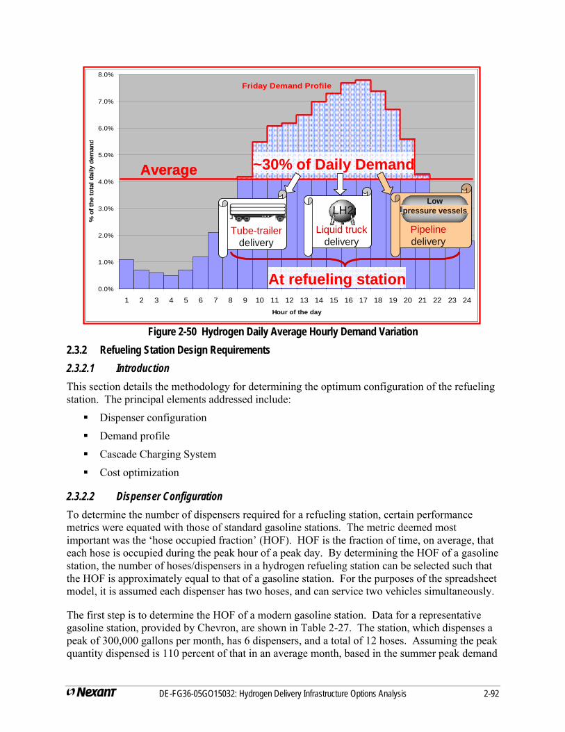
DE-FG36-05GO15032: Hydrogen Delivery Infrastructure Options Analysis 2-92
Friday Demand Profile
0.0%
1.0%
2.0%
3.0%
4.0%
5.0%
6.0%
7.0%
8.0%
1 2 3 4 5 6 7 8 9 10 11 12 13 14 15 16 17 18 19 20 21 22 23 24Hour of the day
% o
f the
tota
l dai
ly d
eman
d
Average ~30% of Daily Demand
LH2
deliveryLiquid truck
Lowpressure vessels
deliveryPipelineTube-trailer
delivery
At refueling station
Friday Demand Profile
0.0%
1.0%
2.0%
3.0%
4.0%
5.0%
6.0%
7.0%
8.0%
1 2 3 4 5 6 7 8 9 10 11 12 13 14 15 16 17 18 19 20 21 22 23 24Hour of the day
% o
f the
tota
l dai
ly d
eman
d
AverageAverage ~30% of Daily Demand~30% of Daily Demand
LH2
deliveryLiquid truck
LH2LH2
deliveryLiquid truck
Lowpressure vessels
deliveryPipeline
Lowpressure vessels
deliveryPipelineTube-trailer
deliveryTube-trailer
delivery
At refueling stationAt refueling station
Figure 2-50 Hydrogen Daily Average Hourly Demand Variation
2.3.2 Refueling Station Design Requirements 2.3.2.1 Introduction This section details the methodology for determining the optimum configuration of the refueling station. The principal elements addressed include:
Dispenser configuration
Demand profile
Cascade Charging System
Cost optimization
2.3.2.2 Dispenser Configuration To determine the number of dispensers required for a refueling station, certain performance metrics were equated with those of standard gasoline stations. The metric deemed most important was the ‘hose occupied fraction’ (HOF). HOF is the fraction of time, on average, that each hose is occupied during the peak hour of a peak day. By determining the HOF of a gasoline station, the number of hoses/dispensers in a hydrogen refueling station can be selected such that the HOF is approximately equal to that of a gasoline station. For the purposes of the spreadsheet model, it is assumed each dispenser has two hoses, and can service two vehicles simultaneously.
The first step is to determine the HOF of a modern gasoline station. Data for a representative gasoline station, provided by Chevron, are shown in Table 2-27. The station, which dispenses a peak of 300,000 gallons per month, has 6 dispensers, and a total of 12 hoses. Assuming the peak quantity dispensed is 110 percent of that in an average month, based in the summer peak demand
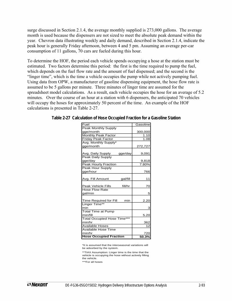
surge discussed in Section 2.1.4, the average monthly supplied is 273,000 gallons. The average month is used because the dispensers are not sized to meet the absolute peak demand within the year. Chevron data illustrating weekly and daily demand, described in Section 2.1.4, indicate the peak hour is generally Friday afternoon, between 4 and 5 pm. Assuming an average per-car consumption of 11 gallons, 70 cars are fueled during this hour.
To determine the HOF, the period each vehicle spends occupying a hose at the station must be estimated. Two factors determine this period: the first is the time required to pump the fuel, which depends on the fuel flow rate and the amount of fuel dispensed; and the second is the “linger time”, which is the time a vehicle occupies the pump while not actively pumping fuel. Using data from OPW, a manufacturer of gasoline dispensing equipment, the hose flow rate is assumed to be 5 gallons per minute. Three minutes of linger time are assumed for the spreadsheet model calculations. As a result, each vehicle occupies the hose for an average of 5.2 minutes. Over the course of an hour at a station with 6 dispensers, the anticipated 70 vehicles will occupy the hoses for approximately 50 percent of the time. An example of the HOF calculations is presented in Table 2-27.
Table 2-27 Calculation of Hose Occupied Fraction for a Gasoline Station Fuel GasolinePeak Monthly Supply gge/month 300,000Monthly Peak Factor 1.10Friday Peak Factor 1.08Avg. Monthly Supply* gge/month 272,727
Avg. Daily Supply gge/day 9,091Peak Daily Supply gge/day 9,818Peak Hourly Fraction 7.80%Peak Hour Supply gge/hour 766
Avg. Fill Amount gal/fill 11
Peak Vehicle Fills fill/hr 70Hose Flow Rate gal/min 5
Time Required for Fill min 2.20Linger Time** min 3Total Time at Pump min/fill 5.20Total Occupied Hose Time*** min/hr 362Available Hoses 12Available Hose Time min/hr 720Hose Occupied Fraction 50.3%
***For all hoses
*It is assumed that the interseasonal variations will be adsorbed by the system.
**TIAX Assumption: Linger time is the time that the vehicle is occupying the hose without actively filling the vehicle.
DE-FG36-05GO15032: Hydrogen Delivery Infrastructure Options Analysis 2-93
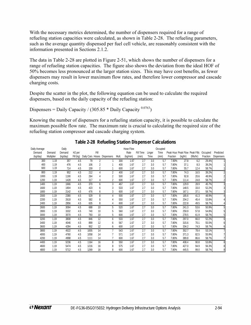
With the necessary metrics determined, the number of dispensers required for a range of refueling station capacities were calculated, as shown in Table 2-28. The refueling parameters, such as the average quantity dispensed per fuel cell vehicle, are reasonably consistent with the information presented in Sections 2.1.2.
The data in Table 2-28 are plotted in Figure 2-51, which shows the number of dispensers for a range of refueling station capacities. The figure also shows the deviation from the ideal HOF of 50% becomes less pronounced at the larger station sizes. This may have cost benefits, as fewer dispensers may result in lower maximum flow rates, and therefore lower compressor and cascade charging costs.
Despite the scatter in the plot, the following equation can be used to calculate the required dispensers, based on the daily capacity of the refueling station:
Dispensers = Daily Capacity / (305.85 * Daily Capacity 0.0763)
Knowing the number of dispensers for a refueling station capacity, it is possible to calculate the maximum possible flow rate. The maximum rate is crucial to calculating the required size of the refueling station compressor and cascade charging system.
Table 2-28 Refueling Station Dispenser Calculations Daily Average
Demand (kg/day)
Demand Multiplier
Daily Demand (kg/day)
H2 per Fill (kg) Daily Cars
Fill Hoses Dispensers Mult.
Hose Flow Rate
(kg/min)Fill Time
(min)Linger Time
Occupied Time (min)
Peak Hour Fraction
Peak Flow (kg/hr)
Peak Fills (fills/hr)
Occupied Fraction
Predicted Dispensers
300 1.19 357 4.5 79 2 1 300 1.67 2.7 3.0 5.7 7.80% 27.8 6.2 29.4% 1400 1.19 476 4.5 106 2 1 400 1.67 2.7 3.0 5.7 7.80% 37.1 8.3 39.2% 1600 1.19 714 4.5 159 2 1 600 1.67 2.7 3.0 5.7 7.80% 55.7 12.4 58.7% 1800 1.19 952 4.5 212 4 2 400 1.67 2.7 3.0 5.7 7.80% 74.3 16.5 39.2% 2
1000 1.19 1190 4.5 264 4 2 500 1.67 2.7 3.0 5.7 7.80% 92.8 20.6 48.9% 21200 1.19 1428 4.5 317 4 2 600 1.67 2.7 3.0 5.7 7.80% 111.4 24.8 58.7% 21400 1.19 1666 4.5 370 6 3 467 1.67 2.7 3.0 5.7 7.80% 129.9 28.9 45.7% 31600 1.19 1904 4.5 423 6 3 533 1.67 2.7 3.0 5.7 7.80% 148.5 33.0 52.2% 31800 1.19 2142 4.5 476 6 3 600 1.67 2.7 3.0 5.7 7.80% 167.1 37.1 58.7% 32000 1.19 2380 4.5 529 8 4 500 1.67 2.7 3.0 5.7 7.80% 185.6 41.3 48.9% 42200 1.19 2618 4.5 582 8 4 550 1.67 2.7 3.0 5.7 7.80% 204.2 45.4 53.8% 42400 1.19 2856 4.5 635 8 4 600 1.67 2.7 3.0 5.7 7.80% 222.8 49.5 58.7% 42600 1.19 3094 4.5 688 10 5 520 1.67 2.7 3.0 5.7 7.80% 241.3 53.6 50.9% 52800 1.19 3332 4.5 740 10 5 560 1.67 2.7 3.0 5.7 7.80% 259.9 57.8 54.8% 53000 1.19 3570 4.5 793 10 5 600 1.67 2.7 3.0 5.7 7.80% 278.5 61.9 58.7% 53200 1.19 3808 4.5 846 12 6 533 1.67 2.7 3.0 5.7 7.80% 297.0 66.0 52.2% 63400 1.19 4046 4.5 899 12 6 567 1.67 2.7 3.0 5.7 7.80% 315.6 70.1 55.5% 63600 1.19 4284 4.5 952 12 6 600 1.67 2.7 3.0 5.7 7.80% 334.2 74.3 58.7% 63800 1.19 4522 4.5 1005 14 7 543 1.67 2.7 3.0 5.7 7.80% 352.7 78.4 53.1% 74000 1.19 4760 4.5 1058 14 7 571 1.67 2.7 3.0 5.7 7.80% 371.3 82.5 55.9% 74200 1.19 4998 4.5 1111 14 7 600 1.67 2.7 3.0 5.7 7.80% 389.8 86.6 58.7% 74400 1.19 5236 4.5 1164 16 8 550 1.67 2.7 3.0 5.7 7.80% 408.4 90.8 53.8% 84600 1.19 5474 4.5 1216 16 8 575 1.67 2.7 3.0 5.7 7.80% 427.0 94.9 56.3% 84800 1.19 5712 4.5 1269 16 8 600 1.67 2.7 3.0 5.7 7.80% 445.5 99.0 58.7% 8
DE-FG36-05GO15032: Hydrogen Delivery Infrastructure Options Analysis 2-94
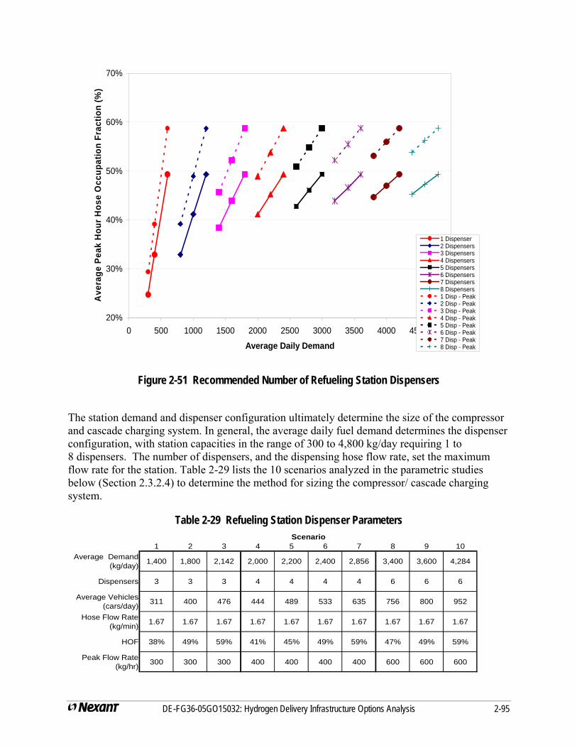
20%
30%
40%
50%
60%
70%
0 500 1000 1500 2000 2500 3000 3500 4000 4500 5000
Average Daily Demand
Ave
rage
Pea
k H
our H
ose
Occ
upat
ion
Frac
tion
(%)
1 Dispenser2 Dispensers3 Dispensers4 Dispensers5 Dispensers6 Dispensers7 Dispensers8 Dispensers1 Disp - Peak2 Disp - Peak3 Disp - Peak4 Disp - Peak5 Disp - Peak6 Disp - Peak7 Disp - Peak8 Disp - Peak
Figure 2-51 Recommended Number of Refueling Station Dispensers
The station demand and dispenser configuration ultimately determine the size of the compressor and cascade charging system. In general, the average daily fuel demand determines the dispenser configuration, with station capacities in the range of 300 to 4,800 kg/day requiring 1 to 8 dispensers. The number of dispensers, and the dispensing hose flow rate, set the maximum flow rate for the station. Table 2-29 lists the 10 scenarios analyzed in the parametric studies below (Section 2.3.2.4) to determine the method for sizing the compressor/ cascade charging system.
Table 2-29 Refueling Station Dispenser Parameters
1 2 3 4 5 6 7 8 9 10Average Demand
(kg/day) 1,400 1,800 2,142 2,000 2,200 2,400 2,856 3,400 3,600 4,284
Dispensers 3 3 3 4 4 4 4 6 6 6
Average Vehicles (cars/day) 311 400 476 444 489 533 635 756 800 952
Hose Flow Rate (kg/min) 1.67 1.67 1.67 1.67 1.67 1.67 1.67 1.67 1.67 1.67
HOF 38% 49% 59% 41% 45% 49% 59% 47% 49% 59%
Peak Flow Rate (kg/hr) 300 300 300 400 400 400 400 600 600 600
Scenario
DE-FG36-05GO15032: Hydrogen Delivery Infrastructure Options Analysis 2-95
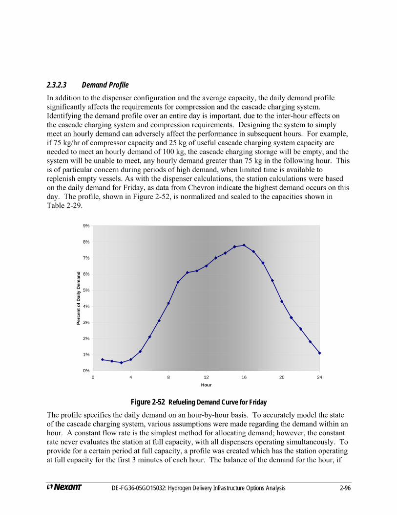
DE-FG36-05GO15032: Hydrogen Delivery Infrastructure Options Analysis 2-96
2.3.2.3 Demand Profile In addition to the dispenser configuration and the average capacity, the daily demand profile significantly affects the requirements for compression and the cascade charging system. Identifying the demand profile over an entire day is important, due to the inter-hour effects on the cascade charging system and compression requirements. Designing the system to simply meet an hourly demand can adversely affect the performance in subsequent hours. For example, if 75 kg/hr of compressor capacity and 25 kg of useful cascade charging system capacity are needed to meet an hourly demand of 100 kg, the cascade charging storage will be empty, and the system will be unable to meet, any hourly demand greater than 75 kg in the following hour. This is of particular concern during periods of high demand, when limited time is available to replenish empty vessels. As with the dispenser calculations, the station calculations were based on the daily demand for Friday, as data from Chevron indicate the highest demand occurs on this day. The profile, shown in Figure 2-52, is normalized and scaled to the capacities shown in Table 2-29.
0%
1%
2%
3%
4%
5%
6%
7%
8%
9%
0 4 8 12 16 20 2
Hour
Perc
ent o
f Dai
ly D
eman
d
4
Figure 2-52 Refueling Demand Curve for Friday
The profile specifies the daily demand on an hour-by-hour basis. To accurately model the state of the cascade charging system, various assumptions were made regarding the demand within an hour. A constant flow rate is the simplest method for allocating demand; however, the constant rate never evaluates the station at full capacity, with all dispensers operating simultaneously. To provide for a certain period at full capacity, a profile was created which has the station operating at full capacity for the first 3 minutes of each hour. The balance of the demand for the hour, if
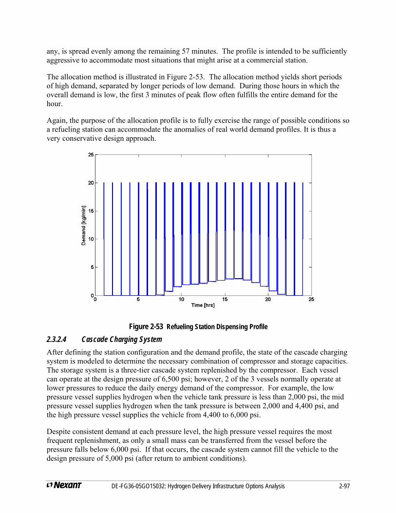
any, is spread evenly among the remaining 57 minutes. The profile is intended to be sufficiently aggressive to accommodate most situations that might arise at a commercial station.
The allocation method is illustrated in Figure 2-53. The allocation method yields short periods of high demand, separated by longer periods of low demand. During those hours in which the overall demand is low, the first 3 minutes of peak flow often fulfills the entire demand for the hour.
Again, the purpose of the allocation profile is to fully exercise the range of possible conditions so a refueling station can accommodate the anomalies of real world demand profiles. It is thus a very conservative design approach.
Figure 2-53 Refueling Station Dispensing Profile 2.3.2.4 Cascade Charging System After defining the station configuration and the demand profile, the state of the cascade charging system is modeled to determine the necessary combination of compressor and storage capacities. The storage system is a three-tier cascade system replenished by the compressor. Each vessel can operate at the design pressure of 6,500 psi; however, 2 of the 3 vessels normally operate at lower pressures to reduce the daily energy demand of the compressor. For example, the low pressure vessel supplies hydrogen when the vehicle tank pressure is less than 2,000 psi, the mid pressure vessel supplies hydrogen when the tank pressure is between 2,000 and 4,400 psi, and the high pressure vessel supplies the vehicle from 4,400 to 6,000 psi.
Despite consistent demand at each pressure level, the high pressure vessel requires the most frequent replenishment, as only a small mass can be transferred from the vessel before the pressure falls below 6,000 psi. If that occurs, the cascade system cannot fill the vehicle to the design pressure of 5,000 psi (after return to ambient conditions).
DE-FG36-05GO15032: Hydrogen Delivery Infrastructure Options Analysis 2-97
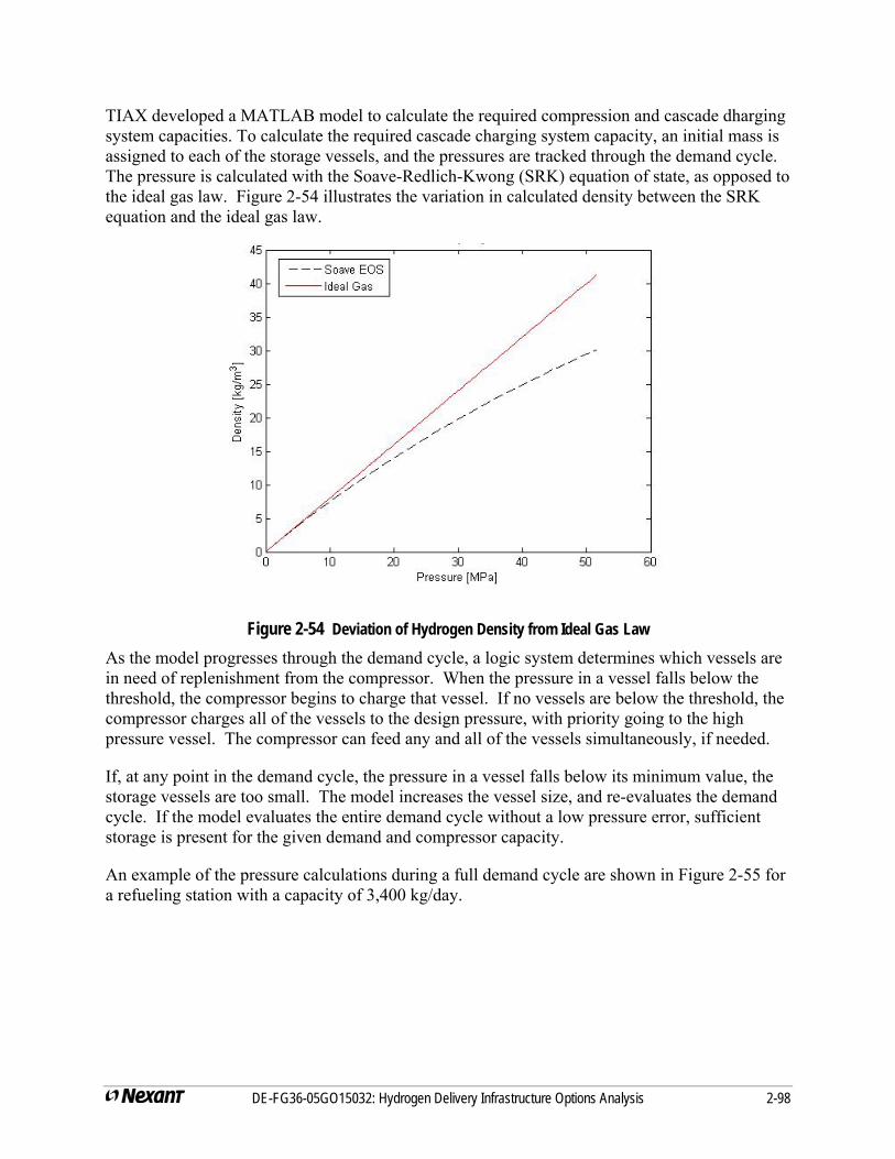
TIAX developed a MATLAB model to calculate the required compression and cascade dharging system capacities. To calculate the required cascade charging system capacity, an initial mass is assigned to each of the storage vessels, and the pressures are tracked through the demand cycle. The pressure is calculated with the Soave-Redlich-Kwong (SRK) equation of state, as opposed to the ideal gas law. Figure 2-54 illustrates the variation in calculated density between the SRK equation and the ideal gas law.
Figure 2-54 Deviation of Hydrogen Density from Ideal Gas Law As the model progresses through the demand cycle, a logic system determines which vessels are in need of replenishment from the compressor. When the pressure in a vessel falls below the threshold, the compressor begins to charge that vessel. If no vessels are below the threshold, the compressor charges all of the vessels to the design pressure, with priority going to the high pressure vessel. The compressor can feed any and all of the vessels simultaneously, if needed.
If, at any point in the demand cycle, the pressure in a vessel falls below its minimum value, the storage vessels are too small. The model increases the vessel size, and re-evaluates the demand cycle. If the model evaluates the entire demand cycle without a low pressure error, sufficient storage is present for the given demand and compressor capacity.
An example of the pressure calculations during a full demand cycle are shown in Figure 2-55 for a refueling station with a capacity of 3,400 kg/day.
DE-FG36-05GO15032: Hydrogen Delivery Infrastructure Options Analysis 2-98
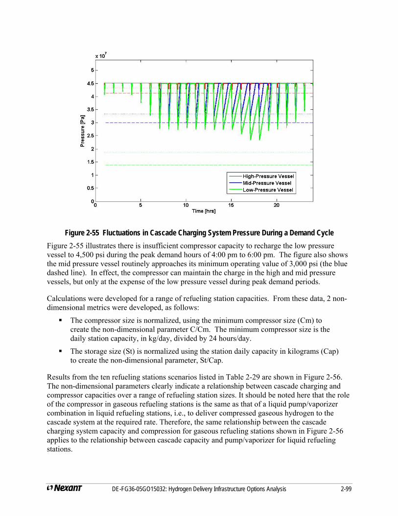
Figure 2-55 Fluctuations in Cascade Charging System Pressure During a Demand Cycle Figure 2-55 illustrates there is insufficient compressor capacity to recharge the low pressure vessel to 4,500 psi during the peak demand hours of 4:00 pm to 6:00 pm. The figure also shows the mid pressure vessel routinely approaches its minimum operating value of 3,000 psi (the blue dashed line). In effect, the compressor can maintain the charge in the high and mid pressure vessels, but only at the expense of the low pressure vessel during peak demand periods.
Calculations were developed for a range of refueling station capacities. From these data, 2 non-dimensional metrics were developed, as follows:
The compressor size is normalized, using the minimum compressor size (Cm) to create the non-dimensional parameter C/Cm. The minimum compressor size is the daily station capacity, in kg/day, divided by 24 hours/day.
The storage size (St) is normalized using the station daily capacity in kilograms (Cap) to create the non-dimensional parameter, St/Cap.
Results from the ten refueling stations scenarios listed in Table 2-29 are shown in Figure 2-56. The non-dimensional parameters clearly indicate a relationship between cascade charging and compressor capacities over a range of refueling station sizes. It should be noted here that the role of the compressor in gaseous refueling stations is the same as that of a liquid pump/vaporizer combination in liquid refueling stations, i.e., to deliver compressed gaseous hydrogen to the cascade system at the required rate. Therefore, the same relationship between the cascade charging system capacity and compression for gaseous refueling stations shown in Figure 2-56 applies to the relationship between cascade capacity and pump/vaporizer for liquid refueling stations.
DE-FG36-05GO15032: Hydrogen Delivery Infrastructure Options Analysis 2-99
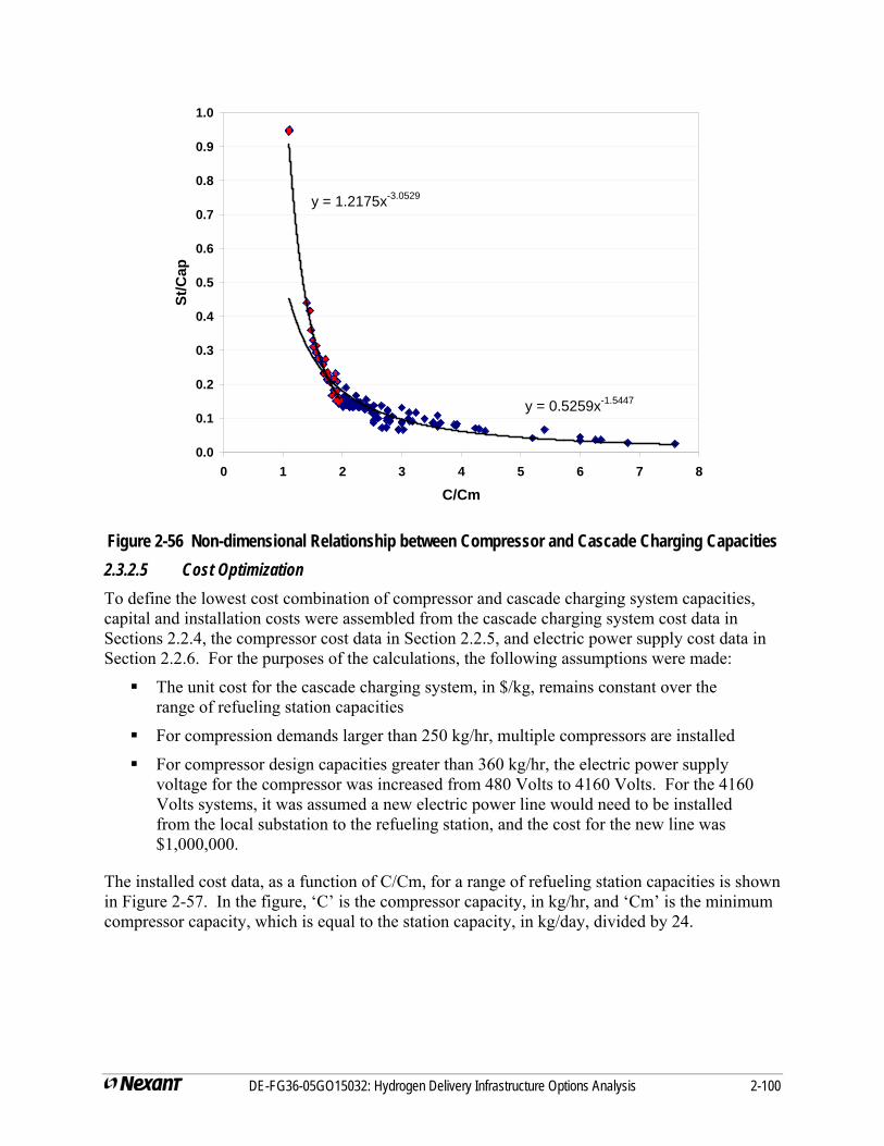
y = 0.5259x-1.5447
y = 1.2175x-3.0529
0.0
0.1
0.2
0.3
0.4
0.5
0.6
0.7
0.8
0.9
1.0
0 1 2 3 4 5 6 7 8
C/Cm
St/C
ap
Figure 2-56 Non-dimensional Relationship between Compressor and Cascade Charging Capacities 2.3.2.5 Cost Optimization To define the lowest cost combination of compressor and cascade charging system capacities, capital and installation costs were assembled from the cascade charging system cost data in Sections 2.2.4, the compressor cost data in Section 2.2.5, and electric power supply cost data in Section 2.2.6. For the purposes of the calculations, the following assumptions were made:
The unit cost for the cascade charging system, in $/kg, remains constant over the range of refueling station capacities
For compression demands larger than 250 kg/hr, multiple compressors are installed
For compressor design capacities greater than 360 kg/hr, the electric power supply voltage for the compressor was increased from 480 Volts to 4160 Volts. For the 4160 Volts systems, it was assumed a new electric power line would need to be installed from the local substation to the refueling station, and the cost for the new line was $1,000,000.
The installed cost data, as a function of C/Cm, for a range of refueling station capacities is shown in Figure 2-57. In the figure, ‘C’ is the compressor capacity, in kg/hr, and ‘Cm’ is the minimum compressor capacity, which is equal to the station capacity, in kg/day, divided by 24.
DE-FG36-05GO15032: Hydrogen Delivery Infrastructure Options Analysis 2-100
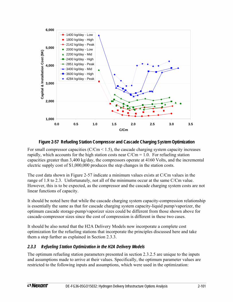
1,000
2,000
3,000
4,000
5,000
6,000
0.0 0.5 1.0 1.5 2.0 2.5 3.0 3.5C/Cm
Cap
ital &
Inst
alla
tion
Cos
t ($K
)
1400 kg/day - Low1800 kg/day - High2142 kg/day - Peak2000 kg/day - Low2200 kg/day - Mid2400 kg/day - High2851 kg/day - Peak3400 kg/day - Mid3600 kg/day - High4284 kg/day - Peak
Figure 2-57 Refueling Station Compressor and Cascade Charging System Optimization For small compressor capacities (C/Cm < 1.5), the cascade charging system capacity increases rapidly, which accounts for the high station costs near C/Cm = 1.0. For refueling station capacities greater than 3,400 kg/day, the compressors operate at 4160 Volts, and the incremental electric supply cost of $1,000,000 produces the step changes in the station costs.
The cost data shown in Figure 2-57 indicate a minimum values exists at C/Cm values in the range of 1.8 to 2.3. Unfortunately, not all of the minimums occur at the same C/Cm value. However, this is to be expected, as the compressor and the cascade charging system costs are not linear functions of capacity.
It should be noted here that while the cascade charging system capacity-compression relationship is essentially the same as that for cascade charging system capacity-liquid pump/vaporizer, the optimum cascade storage-pump/vaporizer sizes could be different from those shown above for cascade-compressor sizes since the cost of compression is different in these two cases.
It should be also noted that the H2A Delivery Models now incorporate a complete cost optimization for the refueling stations that incorporate the principles discussed here and take them a step further as explained in Section 2.3.3.
2.3.3 Refueling Station Optimization in the H2A Delivery Models The optimum refueling station parameters presented in section 2.3.2.5 are unique to the inputs and assumptions made to arrive at their values. Specifically, the optimum parameter values are restricted to the following inputs and assumptions, which were used in the optimization:
DE-FG36-05GO15032: Hydrogen Delivery Infrastructure Options Analysis 2-101
The Chevron daily and hourly demand profiles
The conservative assumed spike in demand at the beginning of each hour
The cost of the compressor, cascade, and electrical upgrades
The minimum and maximum pressures in each of the cascade vessels
The vehicle filling dynamics (tank capacity, fill time, linger time, etc.)
The number of compressors at the refueling station including installed spares
The number of dispensers and the average hose occupied fraction during the peak hour
A calculation methodology has been developed in the H2A Delivery Models V2 to facilitate the analysis of the impact of such inputs on the optimum parameters. The methodology is based on a simple logic, through which the amount of hydrogen and the pressures in each of the cascade vessels are tracked at the critical points of the demand profile, and a decision is made regarding the size of the compressor and cascade system to satisfy such demand with minimum cost. The selected design parameters are those which satisfy the demand profile at all of its critical points.
It should be noted that the calculation methodology in the H2A Delivery Models V2 optimizes the refueling station components by minimizing the total cost contribution of the refueling station to the hydrogen delivery infrastructure rather than minimizing only the compressor and cascade storage system capital costs as adopted in section 2.3.2.5 above. In the H2A Delivery models the cost optimization includes the cost of low pressure storage for (pipeline delivery), power costs for compressors as well as all capital costs. This facilitates the investigation of the demand profile effect on the cost of refueling station storage, the impact of refueling station storage on its land cost, and the effect of possible underutilization of refueling stations in the early market transition period. Furthermore, the methodology is equally applicable to liquid refueling stations in which the cost of liquid pumps and evaporators are considered in place of their compressors counterpart in the gaseous refueling station. Of particular interest to the analysis of the refueling station are the ability to scale or modify the Chevron profile, the ability to scale the demand spike at the first period of each hour by specifying the occupied fraction of hoses during that period, and the ability to specify the number of underutilized stations as a percentage of the number of fully utilized stations in a given market.
A few other particulars of the H2A Delivery Models V2 should also be noted. Although most of the discussions and examples in this report utilize the Chevron 24 hr station fueling profiles, the Models are based on the refueling stations being open 18 hrs (6 AM-Midnight). The 24 hr Chevron fueling profiles are used in the Models neglecting the small discrepancy in that a very small fraction of fueling occurs between midnight and 6 AM. This results in a negligible design inaccuracy of the fueling sites. Also the final fueling time and linger time chosen for use as the defaults in the Models are 2.76 min. and 2.24 min. respectively. It results in the average fill of 4.6 kg of hydrogen (see Section 2.1.2) in 5 minutes of hose occupation time while also satisfying the DOE Hydrogen Program Target of 5 kg filled in 3 minutes.
DE-FG36-05GO15032: Hydrogen Delivery Infrastructure Options Analysis 2-102
2.4 H2A DELIVERY SCENARIO MODEL V2 DELIVERY PATHWAYS 2.4.1 Liquid Pathways Truck delivery of liquid hydrogen from central production to refueling stations in urban areas assumes the city area to be of square boundary and that the refueling stations are uniformly distributed within the city. The distance traveled by the truck within the city boundary to the refueling station is assumed to be 1.5 times the linear dimension of the city. The average roundtrip distance and time can then be calculated based on the distance between the production plant and city gate, the average truck speed on highways and within the city boundary, and the time required to connect, unload, and disconnect at the station. The number of possible truck roundtrips per day can then be calculated from the number of refueling station operating hours per day and the average roundtrip time. Knowing the truck full load capacity and the city peak daily demand, the number of trucks is calculated and scaled.
Process flow diagrams of the three different liquid distribution scenarios modeled are shown in Figure 2-58.
DE-FG36-05GO15032: Hydrogen Delivery Infrastructure Options Analysis 2-103
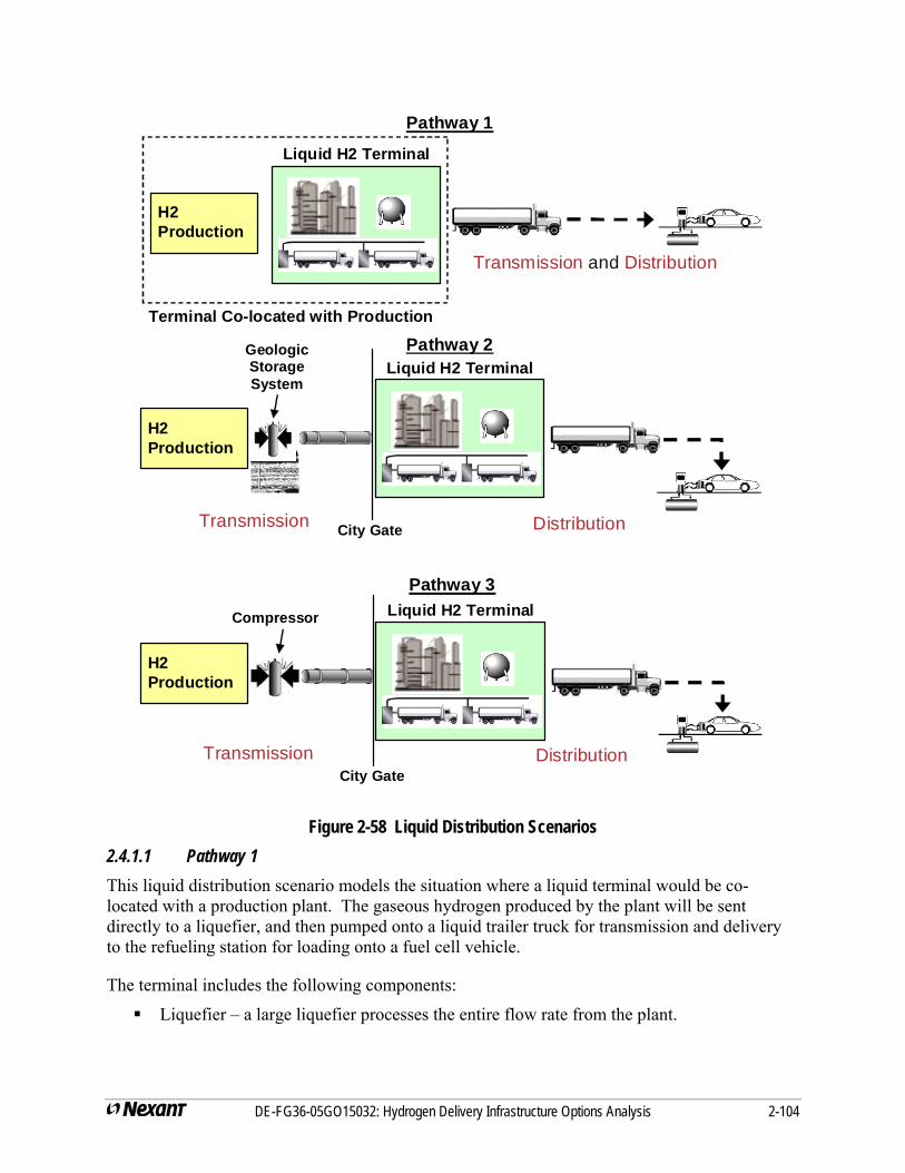
Transmission and Distribution
Pathway 1
H2 Production
Liquid H2 Terminal
Pathway 2 Terminal Co-located with Production
H2 Production
Liquid H2 Terminal
H2 Production
Liquid H2 TerminalPathway 3
City GateTransmission Distribution
City GateTransmission Distribution
Compressor
Geologic Storage System
Figure 2-58 Liquid Distribution Scenarios 2.4.1.1 Pathway 1 This liquid distribution scenario models the situation where a liquid terminal would be co-located with a production plant. The gaseous hydrogen produced by the plant will be sent directly to a liquefier, and then pumped onto a liquid trailer truck for transmission and delivery to the refueling station for loading onto a fuel cell vehicle.
The terminal includes the following components:
Liquefier – a large liquefier processes the entire flow rate from the plant.
DE-FG36-05GO15032: Hydrogen Delivery Infrastructure Options Analysis 2-104
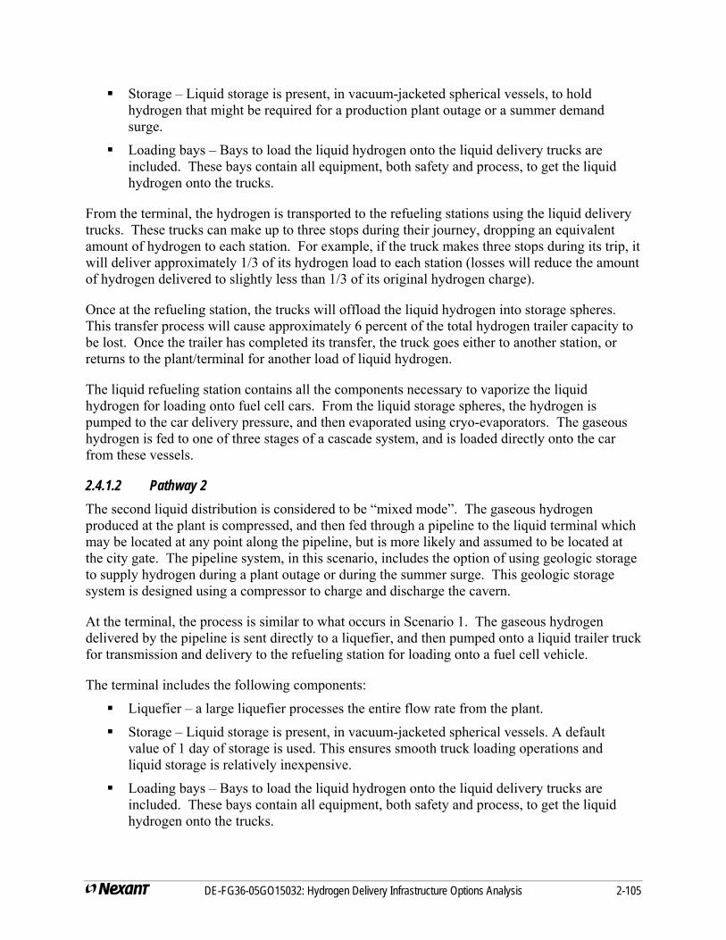
Storage – Liquid storage is present, in vacuum-jacketed spherical vessels, to hold hydrogen that might be required for a production plant outage or a summer demand surge.
Loading bays – Bays to load the liquid hydrogen onto the liquid delivery trucks are included. These bays contain all equipment, both safety and process, to get the liquid hydrogen onto the trucks.
From the terminal, the hydrogen is transported to the refueling stations using the liquid delivery trucks. These trucks can make up to three stops during their journey, dropping an equivalent amount of hydrogen to each station. For example, if the truck makes three stops during its trip, it will deliver approximately 1/3 of its hydrogen load to each station (losses will reduce the amount of hydrogen delivered to slightly less than 1/3 of its original hydrogen charge).
Once at the refueling station, the trucks will offload the liquid hydrogen into storage spheres. This transfer process will cause approximately 6 percent of the total hydrogen trailer capacity to be lost. Once the trailer has completed its transfer, the truck goes either to another station, or returns to the plant/terminal for another load of liquid hydrogen.
The liquid refueling station contains all the components necessary to vaporize the liquid hydrogen for loading onto fuel cell cars. From the liquid storage spheres, the hydrogen is pumped to the car delivery pressure, and then evaporated using cryo-evaporators. The gaseous hydrogen is fed to one of three stages of a cascade system, and is loaded directly onto the car from these vessels.
2.4.1.2 Pathway 2 The second liquid distribution is considered to be “mixed mode”. The gaseous hydrogen produced at the plant is compressed, and then fed through a pipeline to the liquid terminal which may be located at any point along the pipeline, but is more likely and assumed to be located at the city gate. The pipeline system, in this scenario, includes the option of using geologic storage to supply hydrogen during a plant outage or during the summer surge. This geologic storage system is designed using a compressor to charge and discharge the cavern.
At the terminal, the process is similar to what occurs in Scenario 1. The gaseous hydrogen delivered by the pipeline is sent directly to a liquefier, and then pumped onto a liquid trailer truck for transmission and delivery to the refueling station for loading onto a fuel cell vehicle.
The terminal includes the following components:
Liquefier – a large liquefier processes the entire flow rate from the plant.
Storage – Liquid storage is present, in vacuum-jacketed spherical vessels. A default value of 1 day of storage is used. This ensures smooth truck loading operations and liquid storage is relatively inexpensive.
Loading bays – Bays to load the liquid hydrogen onto the liquid delivery trucks are included. These bays contain all equipment, both safety and process, to get the liquid hydrogen onto the trucks.
DE-FG36-05GO15032: Hydrogen Delivery Infrastructure Options Analysis 2-105
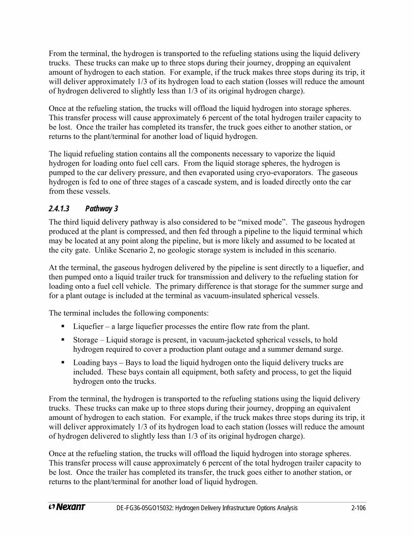
From the terminal, the hydrogen is transported to the refueling stations using the liquid delivery trucks. These trucks can make up to three stops during their journey, dropping an equivalent amount of hydrogen to each station. For example, if the truck makes three stops during its trip, it will deliver approximately 1/3 of its hydrogen load to each station (losses will reduce the amount of hydrogen delivered to slightly less than 1/3 of its original hydrogen charge).
Once at the refueling station, the trucks will offload the liquid hydrogen into storage spheres. This transfer process will cause approximately 6 percent of the total hydrogen trailer capacity to be lost. Once the trailer has completed its transfer, the truck goes either to another station, or returns to the plant/terminal for another load of liquid hydrogen.
The liquid refueling station contains all the components necessary to vaporize the liquid hydrogen for loading onto fuel cell cars. From the liquid storage spheres, the hydrogen is pumped to the car delivery pressure, and then evaporated using cryo-evaporators. The gaseous hydrogen is fed to one of three stages of a cascade system, and is loaded directly onto the car from these vessels.
2.4.1.3 Pathway 3 The third liquid delivery pathway is also considered to be “mixed mode”. The gaseous hydrogen produced at the plant is compressed, and then fed through a pipeline to the liquid terminal which may be located at any point along the pipeline, but is more likely and assumed to be located at the city gate. Unlike Scenario 2, no geologic storage system is included in this scenario.
At the terminal, the gaseous hydrogen delivered by the pipeline is sent directly to a liquefier, and then pumped onto a liquid trailer truck for transmission and delivery to the refueling station for loading onto a fuel cell vehicle. The primary difference is that storage for the summer surge and for a plant outage is included at the terminal as vacuum-insulated spherical vessels.
The terminal includes the following components:
Liquefier – a large liquefier processes the entire flow rate from the plant.
Storage – Liquid storage is present, in vacuum-jacketed spherical vessels, to hold hydrogen required to cover a production plant outage and a summer demand surge.
Loading bays – Bays to load the liquid hydrogen onto the liquid delivery trucks are included. These bays contain all equipment, both safety and process, to get the liquid hydrogen onto the trucks.
From the terminal, the hydrogen is transported to the refueling stations using the liquid delivery trucks. These trucks can make up to three stops during their journey, dropping an equivalent amount of hydrogen to each station. For example, if the truck makes three stops during its trip, it will deliver approximately 1/3 of its hydrogen load to each station (losses will reduce the amount of hydrogen delivered to slightly less than 1/3 of its original hydrogen charge).
Once at the refueling station, the trucks will offload the liquid hydrogen into storage spheres. This transfer process will cause approximately 6 percent of the total hydrogen trailer capacity to be lost. Once the trailer has completed its transfer, the truck goes either to another station, or returns to the plant/terminal for another load of liquid hydrogen.
DE-FG36-05GO15032: Hydrogen Delivery Infrastructure Options Analysis 2-106
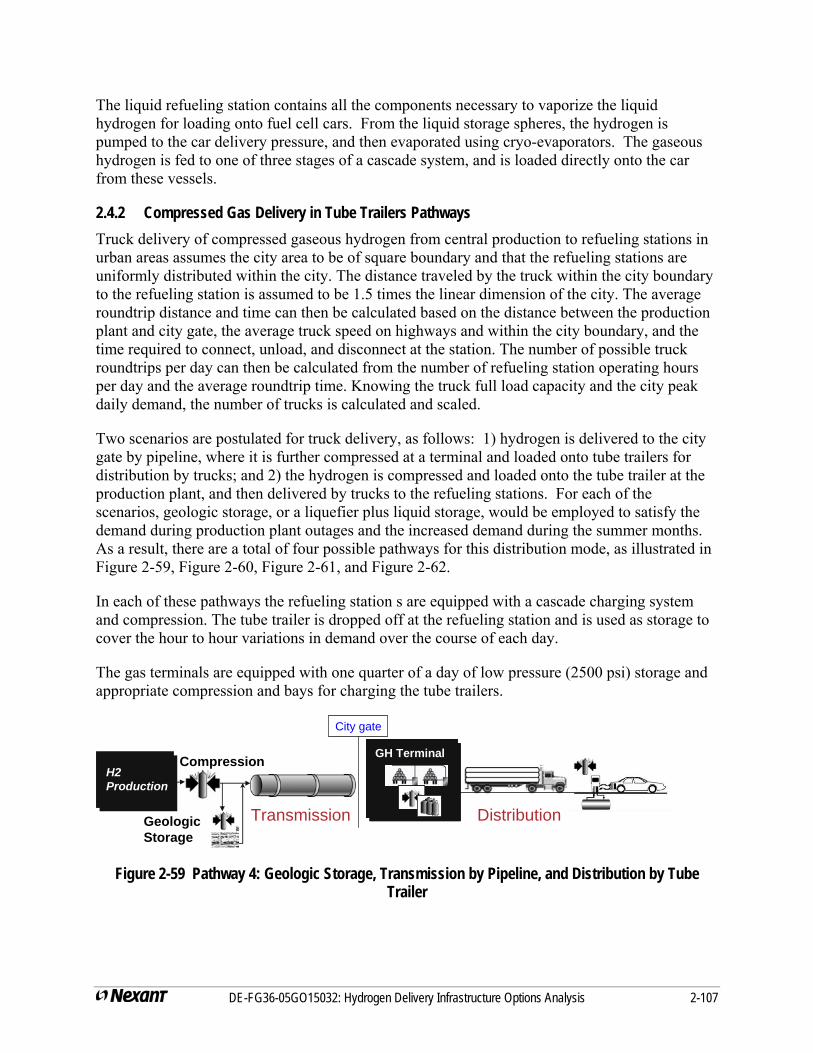
The liquid refueling station contains all the components necessary to vaporize the liquid hydrogen for loading onto fuel cell cars. From the liquid storage spheres, the hydrogen is pumped to the car delivery pressure, and then evaporated using cryo-evaporators. The gaseous hydrogen is fed to one of three stages of a cascade system, and is loaded directly onto the car from these vessels.
2.4.2 Compressed Gas Delivery in Tube Trailers Pathways Truck delivery of compressed gaseous hydrogen from central production to refueling stations in urban areas assumes the city area to be of square boundary and that the refueling stations are uniformly distributed within the city. The distance traveled by the truck within the city boundary to the refueling station is assumed to be 1.5 times the linear dimension of the city. The average roundtrip distance and time can then be calculated based on the distance between the production plant and city gate, the average truck speed on highways and within the city boundary, and the time required to connect, unload, and disconnect at the station. The number of possible truck roundtrips per day can then be calculated from the number of refueling station operating hours per day and the average roundtrip time. Knowing the truck full load capacity and the city peak daily demand, the number of trucks is calculated and scaled.
Two scenarios are postulated for truck delivery, as follows: 1) hydrogen is delivered to the city gate by pipeline, where it is further compressed at a terminal and loaded onto tube trailers for distribution by trucks; and 2) the hydrogen is compressed and loaded onto the tube trailer at the production plant, and then delivered by trucks to the refueling stations. For each of the scenarios, geologic storage, or a liquefier plus liquid storage, would be employed to satisfy the demand during production plant outages and the increased demand during the summer months. As a result, there are a total of four possible pathways for this distribution mode, as illustrated in Figure 2-59, Figure 2-60, Figure 2-61, and Figure 2-62.
In each of these pathways the refueling station s are equipped with a cascade charging system and compression. The tube trailer is dropped off at the refueling station and is used as storage to cover the hour to hour variations in demand over the course of each day.
The gas terminals are equipped with one quarter of a day of low pressure (2500 psi) storage and appropriate compression and bays for charging the tube trailers.
GH TerminalGH TerminalH2 Production
City gate
Transmission Distribution
Compression
Geologic Storage
Figure 2-59 Pathway 4: Geologic Storage, Transmission by Pipeline, and Distribution by Tube Trailer
DE-FG36-05GO15032: Hydrogen Delivery Infrastructure Options Analysis 2-107
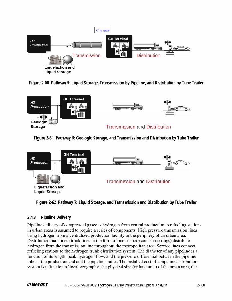
GH TerminalGH TerminalH2 ProductionH2 Production
City gate
Transmission Distribution
Liquefaction and Liquid Storage
Figure 2-60 Pathway 5: Liquid Storage, Transmission by Pipeline, and Distribution by Tube Trailer
GH TerminalGH TerminalH2 ProductionH2 Production
Transmission and Distribution Geologic Storage
Figure 2-61 Pathway 6: Geologic Storage, and Transmission and Distribution by Tube Trailer
H2 ProductionH2 Production
Transmission and Distribution
GH TerminalGH Terminal
Liquefaction and Liquid Storage
Figure 2-62 Pathway 7: Liquid Storage, and Transmission and Distribution by Tube Trailer
2.4.3 Pipeline Delivery Pipeline delivery of compressed gaseous hydrogen from central production to refueling stations in urban areas is assumed to require a series of components. High pressure transmission lines bring hydrogen from a centralized production facility to the periphery of an urban area. Distribution mainlines (trunk lines in the form of one or more concentric rings) distribute hydrogen from the transmission line throughout the metropolitan area. Service lines connect refueling stations to the hydrogen trunk distribution system. The diameter of any pipeline is a function of its length, peak hydrogen flow, and the pressure differential between the pipeline inlet at the production end and the pipeline outlet. The installed cost of a pipeline distribution system is a function of local geography, the physical size (or land area) of the urban area, the
DE-FG36-05GO15032: Hydrogen Delivery Infrastructure Options Analysis 2-108
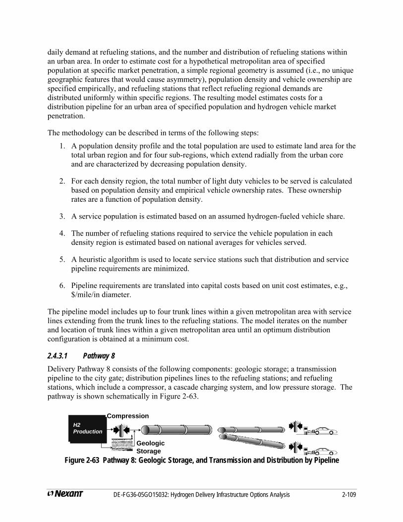
daily demand at refueling stations, and the number and distribution of refueling stations within an urban area. In order to estimate cost for a hypothetical metropolitan area of specified population at specific market penetration, a simple regional geometry is assumed (i.e., no unique geographic features that would cause asymmetry), population density and vehicle ownership are specified empirically, and refueling stations that reflect refueling regional demands are distributed uniformly within specific regions. The resulting model estimates costs for a distribution pipeline for an urban area of specified population and hydrogen vehicle market penetration.
The methodology can be described in terms of the following steps:
1. A population density profile and the total population are used to estimate land area for the total urban region and for four sub-regions, which extend radially from the urban core and are characterized by decreasing population density.
2. For each density region, the total number of light duty vehicles to be served is calculated based on population density and empirical vehicle ownership rates. These ownership rates are a function of population density.
3. A service population is estimated based on an assumed hydrogen-fueled vehicle share.
4. The number of refueling stations required to service the vehicle population in each density region is estimated based on national averages for vehicles served.
5. A heuristic algorithm is used to locate service stations such that distribution and service pipeline requirements are minimized.
6. Pipeline requirements are translated into capital costs based on unit cost estimates, e.g., $/mile/in diameter.
The pipeline model includes up to four trunk lines within a given metropolitan area with service lines extending from the trunk lines to the refueling stations. The model iterates on the number and location of trunk lines within a given metropolitan area until an optimum distribution configuration is obtained at a minimum cost.
2.4.3.1 Pathway 8 Delivery Pathway 8 consists of the following components: geologic storage; a transmission pipeline to the city gate; distribution pipelines lines to the refueling stations; and refueling stations, which include a compressor, a cascade charging system, and low pressure storage. The pathway is shown schematically in Figure 2-63.
H2 ProductionH2 Production
Compression
Figure 2-63 Pathway 8: Geologic Storage, and Transmission and Distribution by Pipeline
Geologic Storage
DE-FG36-05GO15032: Hydrogen Delivery Infrastructure Options Analysis 2-109
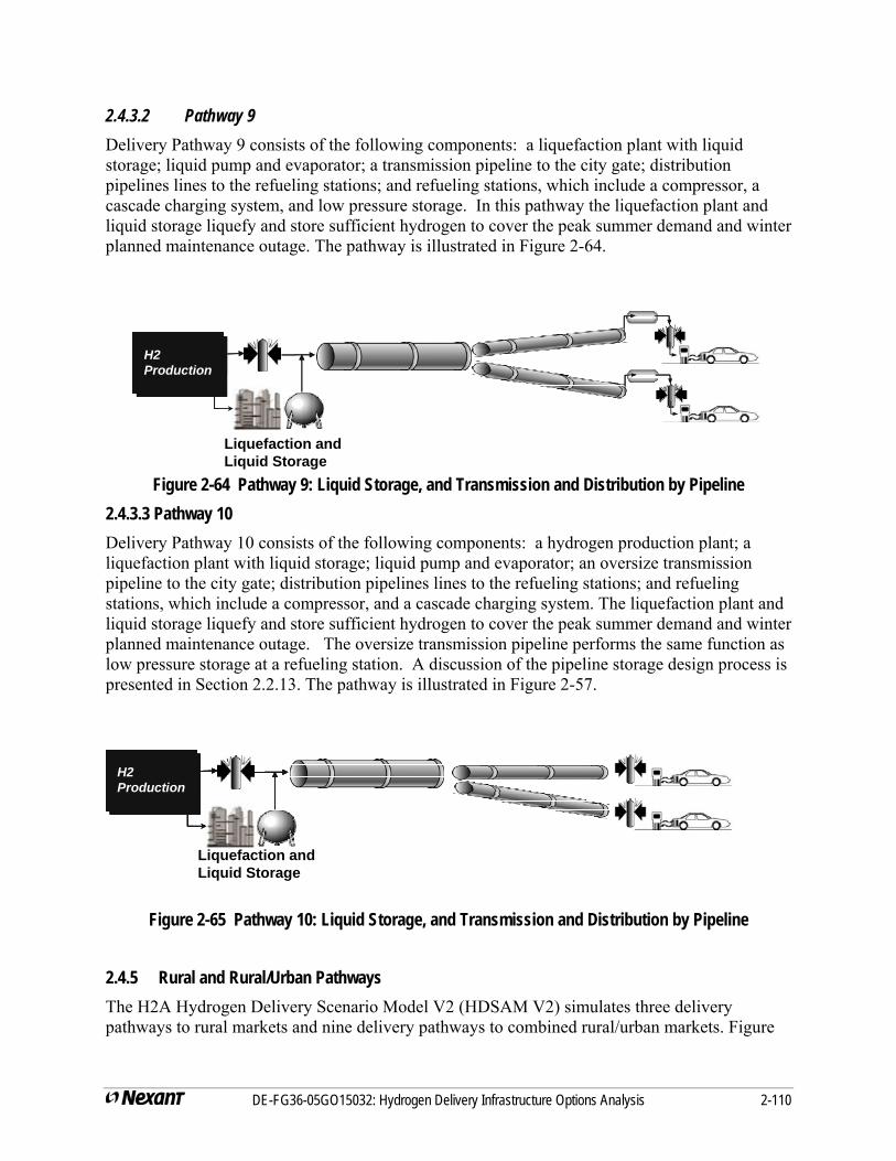
2.4.3.2 Pathway 9 Delivery Pathway 9 consists of the following components: a liquefaction plant with liquid storage; liquid pump and evaporator; a transmission pipeline to the city gate; distribution pipelines lines to the refueling stations; and refueling stations, which include a compressor, a cascade charging system, and low pressure storage. In this pathway the liquefaction plant and liquid storage liquefy and store sufficient hydrogen to cover the peak summer demand and winter planned maintenance outage. The pathway is illustrated in Figure 2-64.
H2 ProductionH2 ProductionH2 Production
Figure 2-64 Pathway 9: Liquid Storage, and Transmission and Distribution by Pipeline
Liquefaction and Liquid Storage
2.4.3.3 Pathway 10 Delivery Pathway 10 consists of the following components: a hydrogen production plant; a liquefaction plant with liquid storage; liquid pump and evaporator; an oversize transmission pipeline to the city gate; distribution pipelines lines to the refueling stations; and refueling stations, which include a compressor, and a cascade charging system. The liquefaction plant and liquid storage liquefy and store sufficient hydrogen to cover the peak summer demand and winter planned maintenance outage. The oversize transmission pipeline performs the same function as low pressure storage at a refueling station. A discussion of the pipeline storage design process is presented in Section 2.2.13. The pathway is illustrated in Figure 2-57.
H2 ProductionH2 ProductionH2 ProductionH2 ProductionH2 Production
Liquefaction and Liquid Storage
Figure 2-65 Pathway 10: Liquid Storage, and Transmission and Distribution by Pipeline
2.4.5 Rural and Rural/Urban Pathways The H2A Hydrogen Delivery Scenario Model V2 (HDSAM V2) simulates three delivery pathways to rural markets and nine delivery pathways to combined rural/urban markets. Figure
DE-FG36-05GO15032: Hydrogen Delivery Infrastructure Options Analysis 2-110
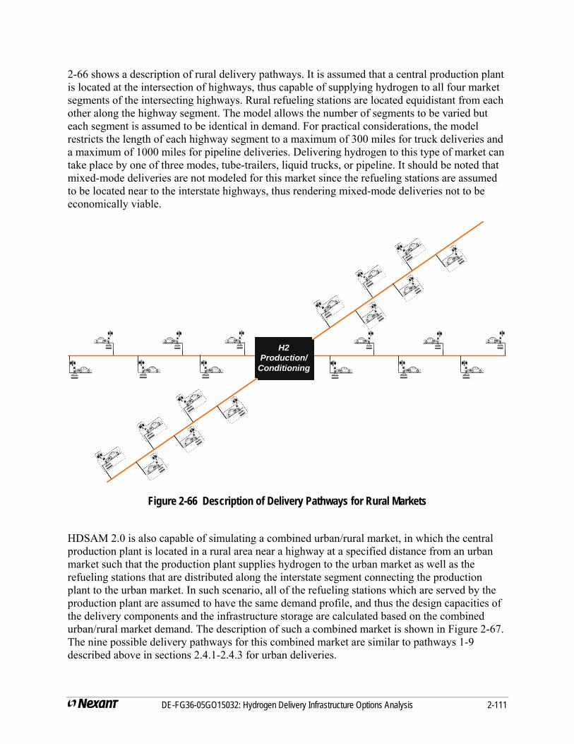
2-66 shows a description of rural delivery pathways. It is assumed that a central production plant is located at the intersection of highways, thus capable of supplying hydrogen to all four market segments of the intersecting highways. Rural refueling stations are located equidistant from each other along the highway segment. The model allows the number of segments to be varied but each segment is assumed to be identical in demand. For practical considerations, the model restricts the length of each highway segment to a maximum of 300 miles for truck deliveries and a maximum of 1000 miles for pipeline deliveries. Delivering hydrogen to this type of market can take place by one of three modes, tube-trailers, liquid trucks, or pipeline. It should be noted that mixed-mode deliveries are not modeled for this market since the refueling stations are assumed to be located near to the interstate highways, thus rendering mixed-mode deliveries not to be economically viable.
H2 Production/
Conditioning
H2 Production/
Conditioning
Figure 2-66 Description of Delivery Pathways for Rural Markets
HDSAM 2.0 is also capable of simulating a combined urban/rural market, in which the central production plant is located in a rural area near a highway at a specified distance from an urban market such that the production plant supplies hydrogen to the urban market as well as the refueling stations that are distributed along the interstate segment connecting the production plant to the urban market. In such scenario, all of the refueling stations which are served by the production plant are assumed to have the same demand profile, and thus the design capacities of the delivery components and the infrastructure storage are calculated based on the combined urban/rural market demand. The description of such a combined market is shown in Figure 2-67. The nine possible delivery pathways for this combined market are similar to pathways 1-9 described above in sections 2.4.1-2.4.3 for urban deliveries.
DE-FG36-05GO15032: Hydrogen Delivery Infrastructure Options Analysis 2-111
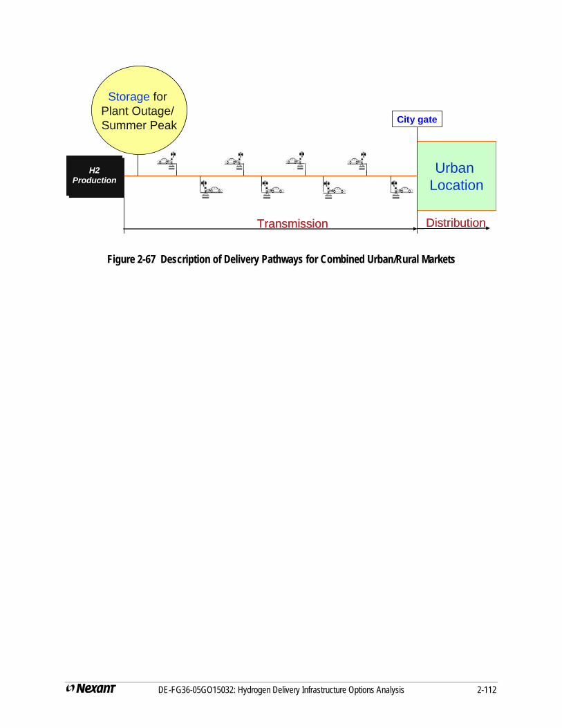
H2 Production
Urban Location
City gate
Transmission Distribution
Storage for Plant Outage/ Summer Peak
H2 Production
Urban Location
City gate
Transmission Distribution
Storage for Plant Outage/ Summer Peak
Figure 2-67 Description of Delivery Pathways for Combined Urban/Rural Markets
DE-FG36-05GO15032: Hydrogen Delivery Infrastructure Options Analysis 2-112
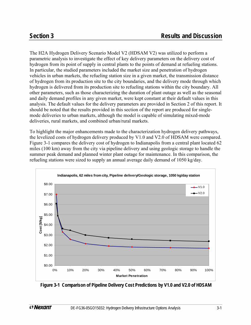
Section 3 Results and Discussion
The H2A Hydrogen Delivery Scenario Model V2 (HDSAM V2) was utilized to perform a parametric analysis to investigate the effect of key delivery parameters on the delivery cost of hydrogen from its point of supply in central plants to the points of demand at refueling stations. In particular, the studied parameters included the market size and penetration of hydrogen vehicles in urban markets, the refueling station size in a given market, the transmission distance of hydrogen from its production site to the city boundaries, and the delivery mode through which hydrogen is delivered from its production site to refueling stations within the city boundary. All other parameters, such as those characterizing the duration of plant outage as well as the seasonal and daily demand profiles in any given market, were kept constant at their default values in this analysis. The default values for the delivery parameters are provided in Section 2 of this report. It should be noted that the results provided in this section of the report are produced for single-mode deliveries to urban markets, although the model is capable of simulating mixed-mode deliveries, rural markets, and combined urban/rural markets.
To highlight the major enhancements made to the characterization hydrogen delivery pathways, the levelized costs of hydrogen delivery produced by V1.0 and V2.0 of HDSAM were compared. Figure 3-1 compares the delivery cost of hydrogen to Indianapolis from a central plant located 62 miles (100 km) away from the city via pipeline delivery and using geologic storage to handle the summer peak demand and planned winter plant outage for maintenance. In this comparison, the refueling stations were sized to supply an annual average daily demand of 1050 kg/day.
Indianapolis, 62 miles from city, Pipeline delivery/Geologic storage, 1050 kg/day station
$0.00
$1.00
$2.00
$3.00
$4.00
$5.00
$6.00
$7.00
$8.00
0% 10% 20% 30% 40% 50% 60% 70% 80% 90% 100%
Market Penetration
Cos
t [$/
kg]
V1.0
V2.0
Figure 3-1 Comparison of Pipeline Delivery Cost Predictions by V1.0 and V2.0 of HDSAM
DE-FG36-05GO15032: Hydrogen Delivery Infrastructure Options Analysis 3-1
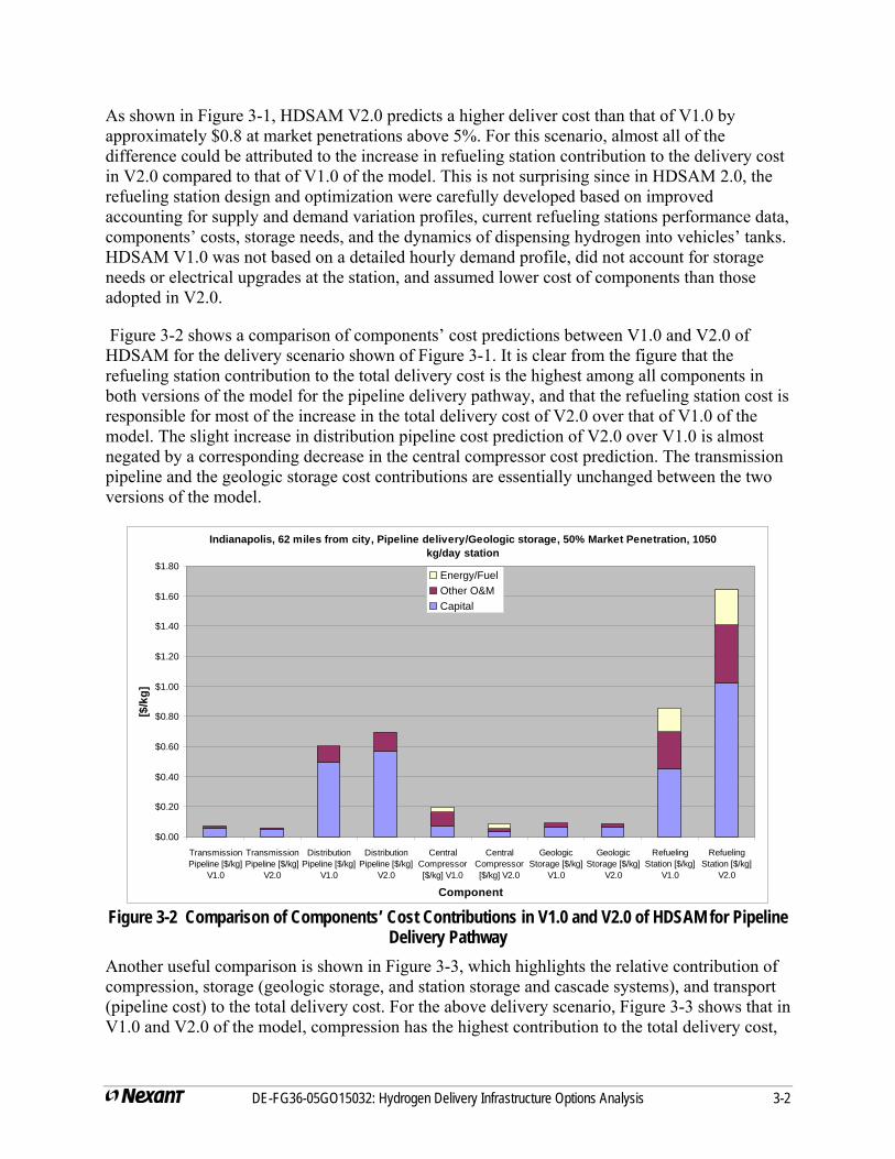
As shown in Figure 3-1, HDSAM V2.0 predicts a higher deliver cost than that of V1.0 by approximately $0.8 at market penetrations above 5%. For this scenario, almost all of the difference could be attributed to the increase in refueling station contribution to the delivery cost in V2.0 compared to that of V1.0 of the model. This is not surprising since in HDSAM 2.0, the refueling station design and optimization were carefully developed based on improved accounting for supply and demand variation profiles, current refueling stations performance data, components’ costs, storage needs, and the dynamics of dispensing hydrogen into vehicles’ tanks. HDSAM V1.0 was not based on a detailed hourly demand profile, did not account for storage needs or electrical upgrades at the station, and assumed lower cost of components than those adopted in V2.0.
Figure 3-2 shows a comparison of components’ cost predictions between V1.0 and V2.0 of HDSAM for the delivery scenario shown of Figure 3-1. It is clear from the figure that the refueling station contribution to the total delivery cost is the highest among all components in both versions of the model for the pipeline delivery pathway, and that the refueling station cost is responsible for most of the increase in the total delivery cost of V2.0 over that of V1.0 of the model. The slight increase in distribution pipeline cost prediction of V2.0 over V1.0 is almost negated by a corresponding decrease in the central compressor cost prediction. The transmission pipeline and the geologic storage cost contributions are essentially unchanged between the two versions of the model.
Indianapolis, 62 miles from city, Pipeline delivery/Geologic storage, 50% Market Penetration, 1050 kg/day station
$0.00
$0.20
$0.40
$0.60
$0.80
$1.00
$1.20
$1.40
$1.60
$1.80
TransmissionPipeline [$/kg]
V1.0
TransmissionPipeline [$/kg]
V2.0
DistributionPipeline [$/kg]
V1.0
DistributionPipeline [$/kg]
V2.0
CentralCompressor[$/kg] V1.0
CentralCompressor[$/kg] V2.0
GeologicStorage [$/kg]
V1.0
GeologicStorage [$/kg]
V2.0
RefuelingStation [$/kg]
V1.0
RefuelingStation [$/kg]
V2.0
Component
[$/k
g]
Energy/Fuel Other O&M Capital
Figure 3-2 Comparison of Components’ Cost Contributions in V1.0 and V2.0 of HDSAM for Pipeline
Delivery Pathway Another useful comparison is shown in Figure 3-3, which highlights the relative contribution of compression, storage (geologic storage, and station storage and cascade systems), and transport (pipeline cost) to the total delivery cost. For the above delivery scenario, Figure 3-3 shows that in V1.0 and V2.0 of the model, compression has the highest contribution to the total delivery cost,
DE-FG36-05GO15032: Hydrogen Delivery Infrastructure Options Analysis 3-2
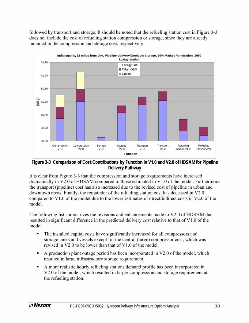
followed by transport and storage. It should be noted that the refueling station cost in Figure 3-3 does not include the cost of refueling station compression or storage, since they are already included in the compression and storage cost, respectively.
Indianapolis, 62 miles from city, Pipeline delivery/Geologic storage, 50% Market Penetration, 1050 kg/day station
$0.00
$0.20
$0.40
$0.60
$0.80
$1.00
$1.20
CompressionV1.0
CompressionV2.0
StorageV1.0
StorageV2.0
TransportV1.0
TransportV2.0
RefuelingStation V1.0
RefuelingStation V2.0
Function
[$/k
g]
Energy/Fuel Other O&M Capital
Figure 3-3 Comparison of Cost Contributions by Function in V1.0 and V2.0 of HDSAM for Pipeline
Delivery Pathway It is clear from Figure 3-3 that the compression and storage requirements have increased dramatically in V2.0 of HDSAM compared to those estimated in V1.0 of the model. Furthermore the transport (pipeline) cost has also increased due to the revised cost of pipeline in urban and downtown areas. Finally, the remainder of the refueling station cost has deceased in V2.0 compared to V1.0 of the model due to the lower estimates of direct/indirect costs in V2.0 of the model.
The following list summarizes the revisions and enhancements made to V2.0 of HDSAM that resulted in significant difference in the predicted delivery cost relative to that of V1.0 of the model.
The installed capital costs have significantly increased for all compressors and storage tanks and vessels except for the central (large) compressor cost, which was revised in V2.0 to be lower than that of V1.0 of the model.
A production plant outage period has been incorporated in V2.0 of the model, which resulted in large infrastructure storage requirement.
A more realistic hourly refueling stations demand profile has been incorporated in V2.0 of the model, which resulted in larger compression and storage requirement at the refueling station.
DE-FG36-05GO15032: Hydrogen Delivery Infrastructure Options Analysis 3-3
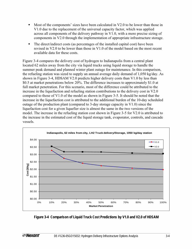
Most of the components’ sizes have been calculated in V2.0 to be lower than those in V1.0 due to the replacement of the universal capacity factor, which was applied across all components of the delivery pathway in V1.0, with a more precise sizing of components in V2.0 through the implementation of appropriate infrastructure storage.
The direct/indirect costs (as percentages of the installed capital cost) have been revised in V2.0 to be lower than those in V1.0 of the model based on the most recent available data for these costs.
Figure 3-4 compares the delivery cost of hydrogen to Indianapolis from a central plant located 62 miles away from the city via liquid trucks using liquid storage to handle the summer peak demand and planned winter plant outage for maintenance. In this comparison, the refueling station was sized to supply an annual average daily demand of 1,050 kg/day. As shown in Figure 3-4, HDSAM V2.0 predicts higher delivery costs than V1.0 by less than $0.5 at market penetrations below 20%. The difference increases to approximately $1.0 at full market penetration. For this scenario, most of the difference could be attributed to the increase in the liquefaction and refueling station contributions to the delivery cost in V2.0 compared to those of V1.0 of the model as shown in Figure 3-5. It should be noted that the increase in the liquefaction cost is attributed to the additional burden of the 10-day scheduled outage of the production plant (compared to 3-day storage capacity in V1.0) since the liquefaction cost for a given liquefier size is almost the same in the two versions of the model. The increase in the refueling station cost shown in Figure 3-5 for V2.0 is attributed to the increase in the estimated cost of the liquid storage tank, evaporator, controls, and cascade vessels.
$0.00
$0.50
$1.00
$1.50
$2.00
$2.50
$3.00
$3.50
$4.00
0% 10% 20% 30% 40% 50% 60% 70% 80% 90% 100%
Cost
[$/k
g]
Market Penetration
Indianapolis, 62 miles from city, LH2 Truck delivery/Storage, 1050 kg/day station
V1.0
V2.0
Figure 3-4 Comparison of Liquid Truck Cost Predictions by V1.0 and V2.0 of HDSAM
DE-FG36-05GO15032: Hydrogen Delivery Infrastructure Options Analysis 3-4
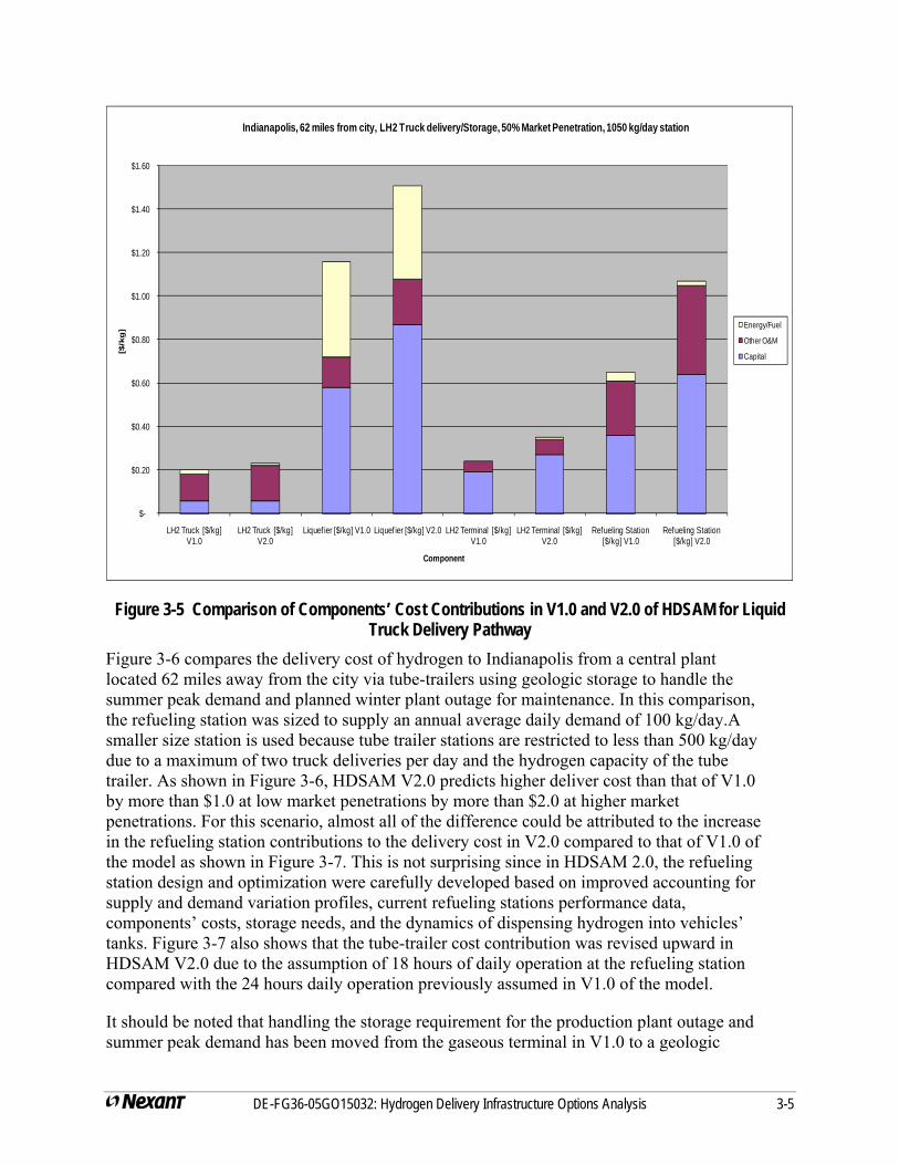
$-
$0.20
$0.40
$0.60
$0.80
$1.00
$1.20
$1.40
$1.60
LH2 Truck [$/kg] V1.0
LH2 Truck [$/kg] V2.0
Liquef ier [$/kg] V1.0 Liquef ier [$/kg] V2.0 LH2 Terminal [$/kg] V1.0
LH2 Terminal [$/kg] V2.0
Refueling Station [$/kg] V1.0
Refueling Station [$/kg] V2.0
[$/k
g]
Component
Indianapolis, 62 miles from city, LH2 Truck delivery/Storage, 50% Market Penetration, 1050 kg/day station
Energy/Fuel
Other O&M
Capital
Figure 3-5 Comparison of Components’ Cost Contributions in V1.0 and V2.0 of HDSAM for Liquid Truck Delivery Pathway
Figure 3-6 compares the delivery cost of hydrogen to Indianapolis from a central plant located 62 miles away from the city via tube-trailers using geologic storage to handle the summer peak demand and planned winter plant outage for maintenance. In this comparison, the refueling station was sized to supply an annual average daily demand of 100 kg/day.A smaller size station is used because tube trailer stations are restricted to less than 500 kg/day due to a maximum of two truck deliveries per day and the hydrogen capacity of the tube trailer. As shown in Figure 3-6, HDSAM V2.0 predicts higher deliver cost than that of V1.0 by more than $1.0 at low market penetrations by more than $2.0 at higher market penetrations. For this scenario, almost all of the difference could be attributed to the increase in the refueling station contributions to the delivery cost in V2.0 compared to that of V1.0 of the model as shown in Figure 3-7. This is not surprising since in HDSAM 2.0, the refueling station design and optimization were carefully developed based on improved accounting for supply and demand variation profiles, current refueling stations performance data, components’ costs, storage needs, and the dynamics of dispensing hydrogen into vehicles’ tanks. Figure 3-7 also shows that the tube-trailer cost contribution was revised upward in HDSAM V2.0 due to the assumption of 18 hours of daily operation at the refueling station compared with the 24 hours daily operation previously assumed in V1.0 of the model.
It should be noted that handling the storage requirement for the production plant outage and summer peak demand has been moved from the gaseous terminal in V1.0 to a geologic
DE-FG36-05GO15032: Hydrogen Delivery Infrastructure Options Analysis 3-5
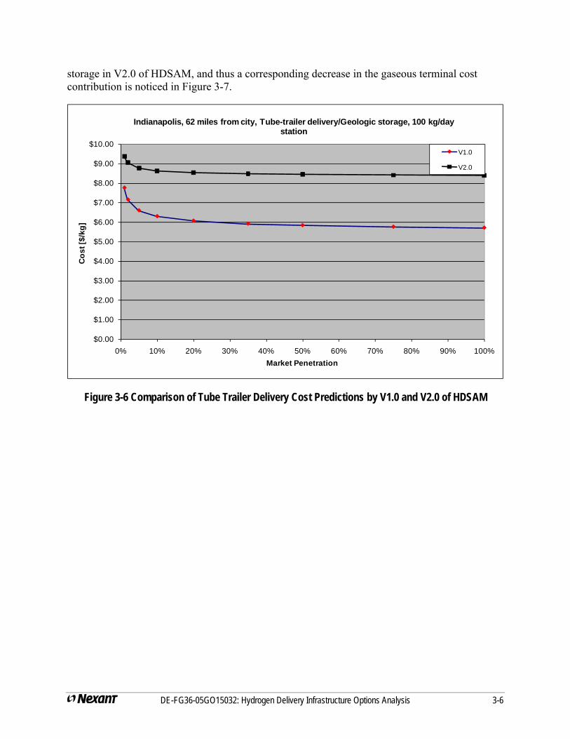
storage in V2.0 of HDSAM, and thus a corresponding decrease in the gaseous terminal cost contribution is noticed in Figure 3-7.
$0.00
$1.00
$2.00
$3.00
$4.00
$5.00
$6.00
$7.00
$8.00
$9.00
$10.00
0% 10% 20% 30% 40% 50% 60% 70% 80% 90% 100%
Cos
t [$/
kg]
Market Penetration
Indianapolis, 62 miles from city, Tube-trailer delivery/Geologic storage, 100 kg/day station
V1.0
V2.0
Figure 3-6 Comparison of Tube Trailer Delivery Cost Predictions by V1.0 and V2.0 of HDSAM
DE-FG36-05GO15032: Hydrogen Delivery Infrastructure Options Analysis 3-6
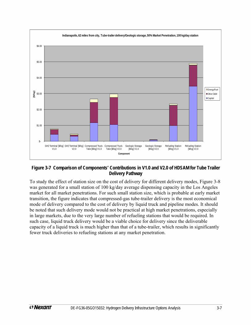
DE-FG36-05GO15032: Hydrogen Delivery Infrastructure Options Analysis 3-7
$-
$1.00
$2.00
$3.00
$4.00
$5.00
$6.00
GH2 Terminal [$/kg] V1.0
GH2 Terminal [$/kg] V2.0
Compressed Truck-Tube [$/kg] V1.0
Compressed Truck-Tube [$/kg] V2.0
Geologic Storage [$/kg] V1.0
Geologic Storage [$/kg] V2.0
Refueling Station [$/kg] V1.0
Refueling Station [$/kg] V2.0
[$/k
g]
Component
Indianapolis, 62 miles from city, Tube-trailer delivery/Geologic storage, 50% Market Penetration, 100 kg/day station
Energy/Fuel
Other O&M
Capital
Figure 3-7 Comparison of Components’ Contributions in V1.0 and V2.0 of HDSAM for Tube Trailer Delivery Pathway
To study the effect of station size on the cost of delivery for different delivery modes, Figure 3was generated for a small station of 100 kg/day average dispensing capacity in the Los Amarket for all market penetrations. For such small station size, which is probable at early market transition, the figure indicates that compressed-gas tube-trailer delivery is the most economical mode of delivery compared to the cost of delivery by liquid truck and pipeline modes. It shoube noted that such delivery mode would not be practical at high market penetrations, especin large markets, due to the very large number of refueling stations that would be required. In such case, liquid truck delivery would be a viable choice for delivery since the deliverable capacity of a liquid truck is much higher than that of a tube-trailer, which results in significantlyfewer truck deliveries to refueling stations at any market penetration.
-8 ngeles
ld ially
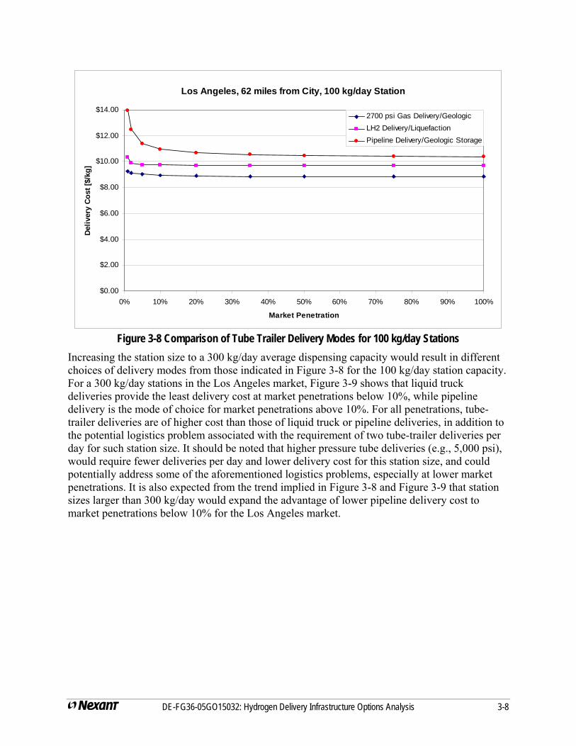
DE-FG36-05GO15032: Hydrogen Delivery Infrastructure Options Analysis 3-8
Los Angeles, 62 miles from City, 100 kg/day Station
$0.00
$2.00
$4.00
$6.00
$8.00
$10.00
$12.00
$14.00
0% 10% 20% 30% 40% 50% 60% 70% 80% 90% 100%
Market Penetration
Deliv
ery
Cost
[$/k
g]
2700 psi Gas Delivery/GeologicLH2 Delivery/LiquefactionPipeline Delivery/Geologic Storage
Figure 3-8 Comparison of Tube Trailer Delivery Modes for 100 kg/day Stations
Increasing the station size to a 300 kg/day average dispensing capacity would result in different choices of delivery modes from those indicated in Figure 3-8 for the 100 kg/day station capacity. For a 300 kg/day stations in the Los Angeles market, Figure 3-9 shows that liquid truck deliveries provide the least delivery cost at market penetrations below 10%, while pipeline delivery is the mode of choice for market penetrations above 10%. For all penetrations, tube-trailer deliveries are of higher cost than those of liquid truck or pipeline deliveries, in addition to the potential logistics problem associated with the requirement of two tube-trailer deliveries pday for such station size. It should be noted that higher pressure tube deliveries (e.g., 5,000 pwould require fewer deliveries per day and lower delivery cost for this station size, and could potentially address some of the aforementioned logistics problems, especially at lower penetrations. It is also expected from the trend implied in Figure 3-8 and Figure 3-9 that stationsizes larger than 300 kg/day would expand the advantage of lower pipeline delivery cost to market penetrations below 10% for the Los Angeles market.
er si),
market
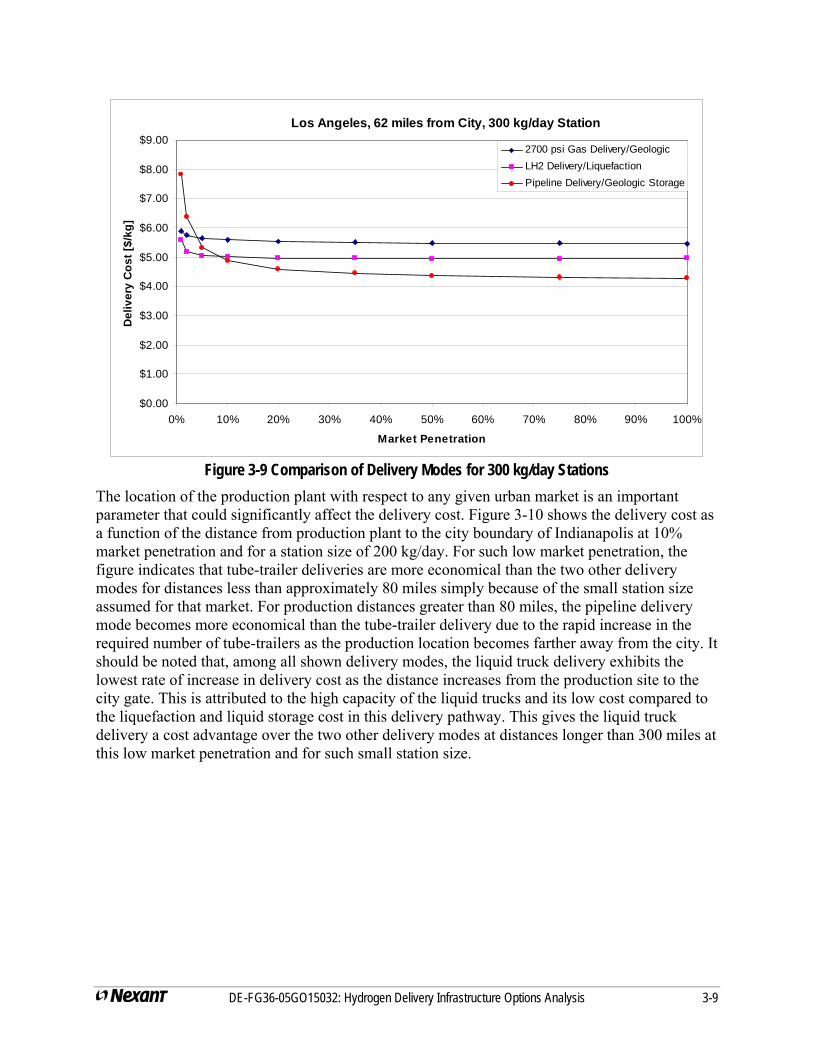
DE-FG36-05GO15032: Hydrogen Delivery Infrastructure Options Analysis 3-9
Los Angeles, 62 miles from City, 300 kg/day Station
$0.00
$1.00
$2.00
$3.00
$4.00
$5.00
$6.00
$7.00
$8.00
$9.00
0% 10% 20% 30% 40% 50% 60% 70% 80% 90% 100%
Market Penetration
Del
iver
y C
ost [
$/kg
]
2700 psi Gas Delivery/GeologicLH2 Delivery/LiquefactionPipeline Delivery/Geologic Storage
Figure 3-9 Comparison of Delivery Modes for 300 kg/day Stations
The location of the production plant with respect to any given urban market is an important parameter that could significantly affect the delivery cost. Figure 3-10 shows the deliverya function of the distance from production plant to the city boundary of Indianapolis at 10% market penetration and for a station size of 200 kg/day. For such low market penetration, the figure indicates that tube-trailer deliveries are more economical than the two other delivery modes for distances less than approximately 80 miles simply because of the small station size assumed for that market. For production distances greater than 80 miles, the pipeline delivery mode becomes more economical than the tube-trailer delivery due to the rapid increase in the required number of tube-trailers as the production location becomes farther away from the city. Itshould be noted that, among all shown delivery modes, the liquid truck delivery exhibits the lowest rate of increase in delivery cost as the distance increases from the production site to the city gate. This is attributed to the high capacity of the liquid trucks and its low cost compared to the liquefaction and liquid storage cost in this delivery pathway. This gives the liquid truck delivery a cost advantage over the two other delivery modes at distances longer than 300 miles athis low market penetration and for such small station size.
cost as
t
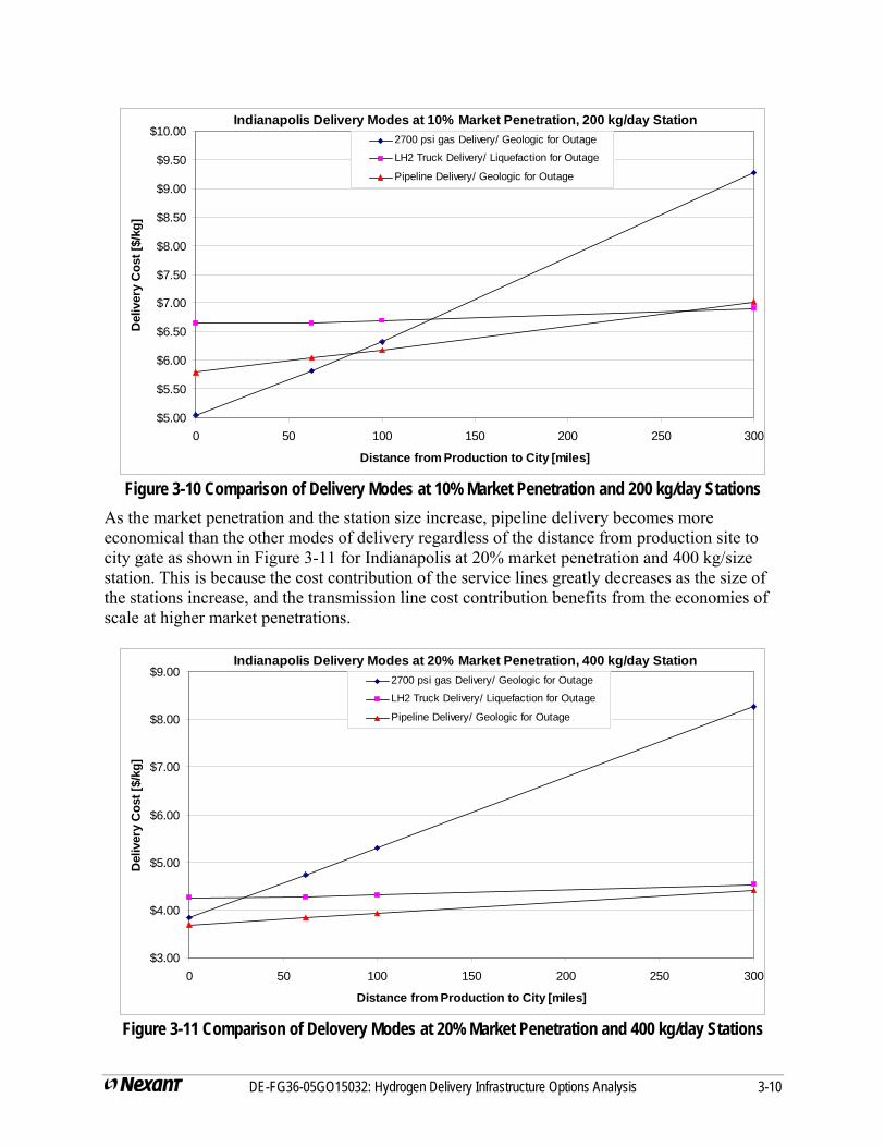
DE-FG36-05GO15032: Hydrogen Delivery Infrastructure Options Analysis 3-10
Indianapolis Delivery Modes at 10% Market Penetration, 200 kg/day Station
$5.00
$5.50
$6.00
$6.50
$7.00
$7.50
$8.00
$8.50
$9.00
$9.50
$10.00
0 50 100 150 200 250 300
Distance from Production to City [miles]
Del
iver
y C
ost [
$/kg
]2700 psi gas Delivery/ Geologic for Outage
LH2 Truck Delivery/ Liquefaction for Outage
Pipeline Delivery/ Geologic for Outage
Figure 3-10 Comparison of Delivery Modes at 10% Market Penetration and 200 kg/day Stations
As the market penetration and the station size increase, pipeline delivery becomes more economical than the other modes of delivery regardless of the distance from production site to city gate as shown in Figure 3-11 for Indianapolis at 20% market penetration and 400 kg/size station. This is because the cost contribution of the service lines greatly decreases as the size the stations increase, and the transmission line cost contribution benefits from the economies of scale at higher market penetrations.
of
Indianapolis Delivery Modes at 20% Market Penetration, 400 kg/day Station
$3.00
$4.00
$5.00
$6.00
$7.00
$8.00
$9.00
0 50 100 150 200 250 300
Distance from Production to City [miles]
Del
iver
y C
ost [
$/kg
]
2700 psi gas Delivery/ Geologic for Outage
LH2 Truck Delivery/ Liquefaction for Outage
Pipeline Delivery/ Geologic for Outage
Figure 3-11 Comparison of Delovery Modes at 20% Market Penetration and 400 kg/day Stations
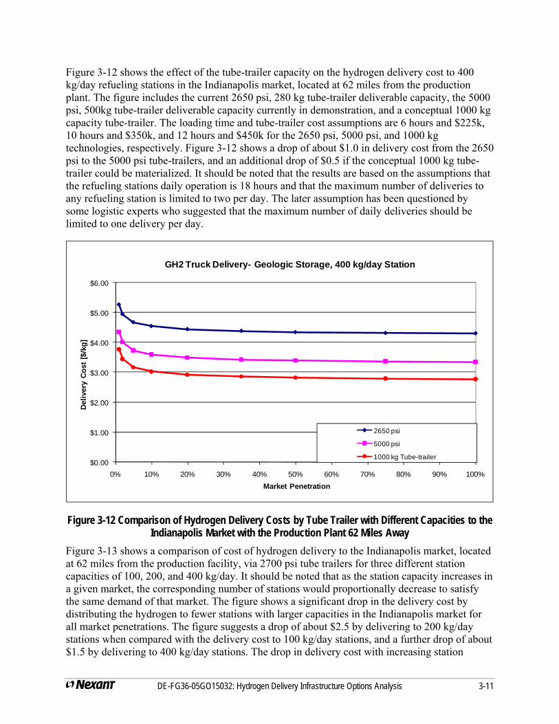
Figure 3-12 shows the effect of the tube-trailer capacity on the hydrogen delivery cost to 400 kg/day refueling stations in the Indianapolis market, located at 62 miles from the production plant. The figure includes the current 2650 psi, 280 kg tube-trailer deliverable capacity, the 5000 psi, 500kg tube-trailer deliverable capacity currently in demonstration, and a conceptual 1000 kg capacity tube-trailer. The loading time and tube-trailer cost assumptions are 6 hours and $225k, 10 hours and $350k, and 12 hours and $450k for the 2650 psi, 5000 psi, and 1000 kg technologies, respectively. Figure 3-12 shows a drop of about $1.0 in delivery cost from the 2650 psi to the 5000 psi tube-trailers, and an additional drop of $0.5 if the conceptual 1000 kg tube-trailer could be materialized. It should be noted that the results are based on the assumptions that the refueling stations daily operation is 18 hours and that the maximum number of deliveries to any refueling station is limited to two per day. The later assumption has been questioned by some logistic experts who suggested that the maximum number of daily deliveries should be limited to one delivery per day.
$0.00
$1.00
$2.00
$3.00
$4.00
$5.00
$6.00
0% 10% 20% 30% 40% 50% 60% 70% 80% 90% 100%
Deliv
ery
Cost
[$/k
g]
Market Penetration
GH2 Truck Delivery- Geologic Storage, 400 kg/day Station
2650 psi
5000 psi
1000 kg Tube-trailer
Figure 3-12 Comparison of Hydrogen Delivery Costs by Tube Trailer with Different Capacities to the Indianapolis Market with the Production Plant 62 Miles Away
Figure 3-13 shows a comparison of cost of hydrogen delivery to the Indianapolis market, located at 62 miles from the production facility, via 2700 psi tube trailers for three different station capacities of 100, 200, and 400 kg/day. It should be noted that as the station capacity increases in a given market, the corresponding number of stations would proportionally decrease to satisfy the same demand of that market. The figure shows a significant drop in the delivery cost by distributing the hydrogen to fewer stations with larger capacities in the Indianapolis market for all market penetrations. The figure suggests a drop of about $2.5 by delivering to 200 kg/day stations when compared with the delivery cost to 100 kg/day stations, and a further drop of about $1.5 by delivering to 400 kg/day stations. The drop in delivery cost with increasing station
DE-FG36-05GO15032: Hydrogen Delivery Infrastructure Options Analysis 3-11
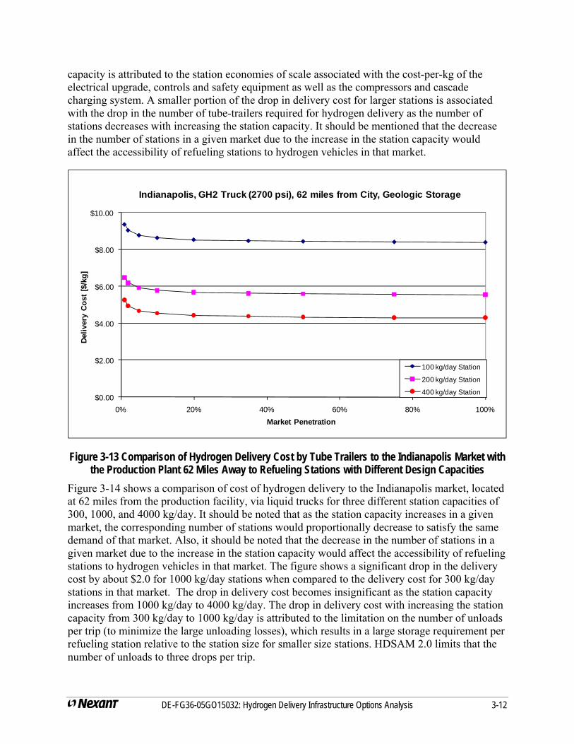
capacity is attributed to the station economies of scale associated with the cost-per-kg of the electrical upgrade, controls and safety equipment as well as the compressors and cascade charging system. A smaller portion of the drop in delivery cost for larger stations is associated with the drop in the number of tube-trailers required for hydrogen delivery as the number of stations decreases with increasing the station capacity. It should be mentioned that the decrease in the number of stations in a given market due to the increase in the station capacity would affect the accessibility of refueling stations to hydrogen vehicles in that market.
$0.00
$2.00
$4.00
$6.00
$8.00
$10.00
0% 20% 40% 60% 80% 100%
Deliv
ery
Cost
[$/k
g]
Market Penetration
Indianapolis, GH2 Truck (2700 psi), 62 miles from City, Geologic Storage
100 kg/day Station
200 kg/day Station
400 kg/day Station
Figure 3-13 Comparison of Hydrogen Delivery Cost by Tube Trailers to the Indianapolis Market with the Production Plant 62 Miles Away to Refueling Stations with Different Design Capacities
Figure 3-14 shows a comparison of cost of hydrogen delivery to the Indianapolis market, located at 62 miles from the production facility, via liquid trucks for three different station capacities of 300, 1000, and 4000 kg/day. It should be noted that as the station capacity increases in a given market, the corresponding number of stations would proportionally decrease to satisfy the same demand of that market. Also, it should be noted that the decrease in the number of stations in a given market due to the increase in the station capacity would affect the accessibility of refueling stations to hydrogen vehicles in that market. The figure shows a significant drop in the delivery cost by about $2.0 for 1000 kg/day stations when compared to the delivery cost for 300 kg/day stations in that market. The drop in delivery cost becomes insignificant as the station capacity increases from 1000 kg/day to 4000 kg/day. The drop in delivery cost with increasing the station capacity from 300 kg/day to 1000 kg/day is attributed to the limitation on the number of unloads per trip (to minimize the large unloading losses), which results in a large storage requirement per refueling station relative to the station size for smaller size stations. HDSAM 2.0 limits that the number of unloads to three drops per trip.
DE-FG36-05GO15032: Hydrogen Delivery Infrastructure Options Analysis 3-12
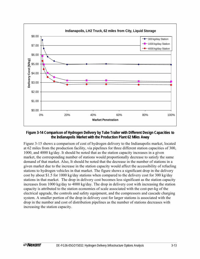
$0.00
$1.00
$2.00
$3.00
$4.00
$5.00
$6.00
$7.00
$8.00
0% 20% 40% 60% 80% 100%
Del
iver
y C
ost
[$/k
g]
Market Penetration
Indianapolis, LH2 Truck, 62 miles from City, Liquid Storage
300 kg/day Station
1000 kg/day Station
4000 kg/day Station
Figure 3-14 Comparison of Hydrogen Delivery by Tube Trailer with Different Design Capacities to the Indianapolis Market with the Production Plant 62 Miles Away
Figure 3-15 shows a comparison of cost of hydrogen delivery to the Indianapolis market, located at 62 miles from the production facility, via pipelines for three different station capacities of 300, 1000, and 4000 kg/day. It should be noted that as the station capacity increases in a given market, the corresponding number of stations would proportionally decrease to satisfy the same demand of that market. Also, It should be noted that the decrease in the number of stations in a given market due to the increase in the station capacity would affect the accessibility of refueling stations to hydrogen vehicles in that market. The figure shows a significant drop in the delivery cost by about $1.5 for 1000 kg/day stations when compared to the delivery cost for 300 kg/day stations in that market. The drop in delivery cost becomes less significant as the station capacity increases from 1000 kg/day to 4000 kg/day. The drop in delivery cost with increasing the station capacity is attributed to the station economies of scale associated with the cost-per-kg of the electrical upgrade, the controls and safety equipment, and the compressors and cascade charging system. A smaller portion of the drop in delivery cost for larger stations is associated with the drop in the number and cost of distribution pipelines as the number of stations decreases with increasing the station capacity.
DE-FG36-05GO15032: Hydrogen Delivery Infrastructure Options Analysis 3-13
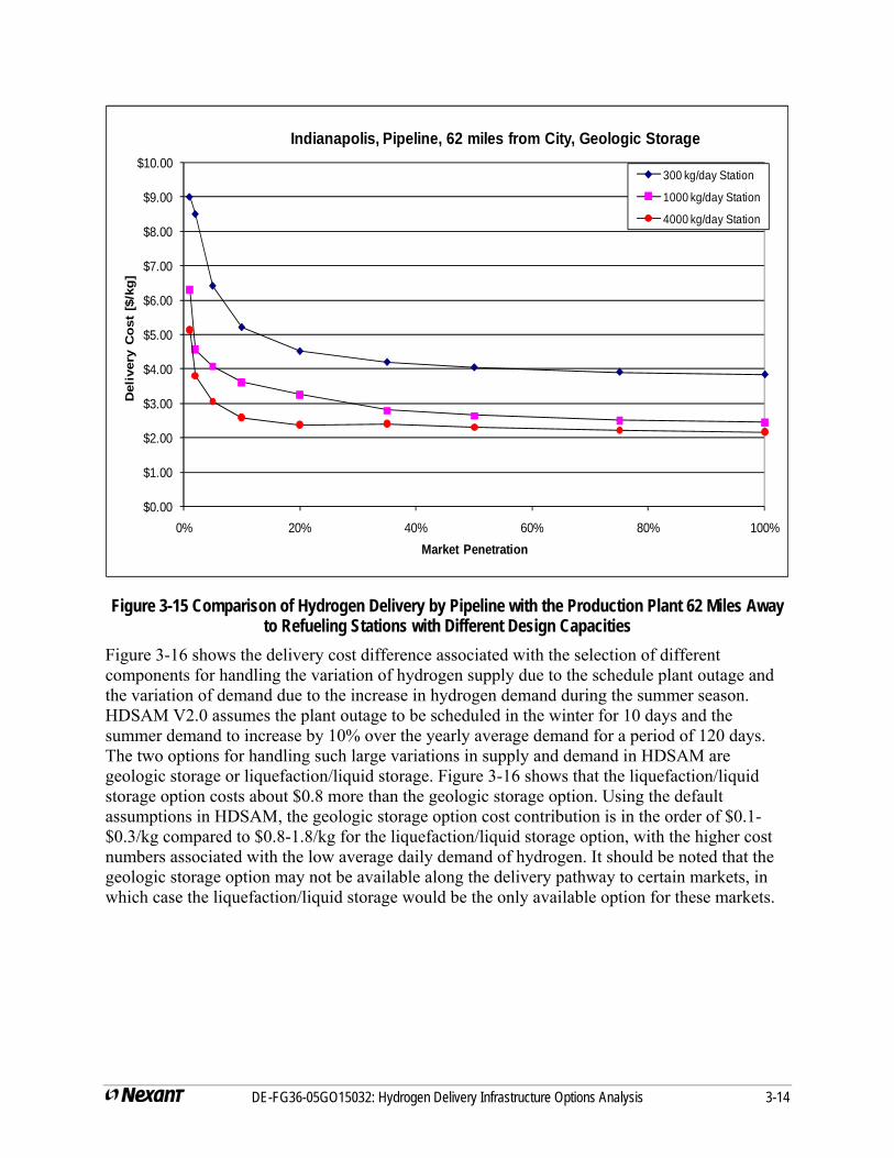
$0.00
$1.00
$2.00
$3.00
$4.00
$5.00
$6.00
$7.00
$8.00
$9.00
$10.00
0% 20% 40% 60% 80% 100%
Del
iver
y C
ost
[$/k
g]
Market Penetration
Indianapolis, Pipeline, 62 miles from City, Geologic Storage
300 kg/day Station
1000 kg/day Station
4000 kg/day Station
Figure 3-15 Comparison of Hydrogen Delivery by Pipeline with the Production Plant 62 Miles Away to Refueling Stations with Different Design Capacities
Figure 3-16 shows the delivery cost difference associated with the selection of different components for handling the variation of hydrogen supply due to the schedule plant outage and the variation of demand due to the increase in hydrogen demand during the summer season. HDSAM V2.0 assumes the plant outage to be scheduled in the winter for 10 days and the summer demand to increase by 10% over the yearly average demand for a period of 120 days. The two options for handling such large variations in supply and demand in HDSAM are geologic storage or liquefaction/liquid storage. Figure 3-16 shows that the liquefaction/liquid storage option costs about $0.8 more than the geologic storage option. Using the default assumptions in HDSAM, the geologic storage option cost contribution is in the order of $0.1-$0.3/kg compared to $0.8-1.8/kg for the liquefaction/liquid storage option, with the higher cost numbers associated with the low average daily demand of hydrogen. It should be noted that the geologic storage option may not be available along the delivery pathway to certain markets, in which case the liquefaction/liquid storage would be the only available option for these markets.
DE-FG36-05GO15032: Hydrogen Delivery Infrastructure Options Analysis 3-14
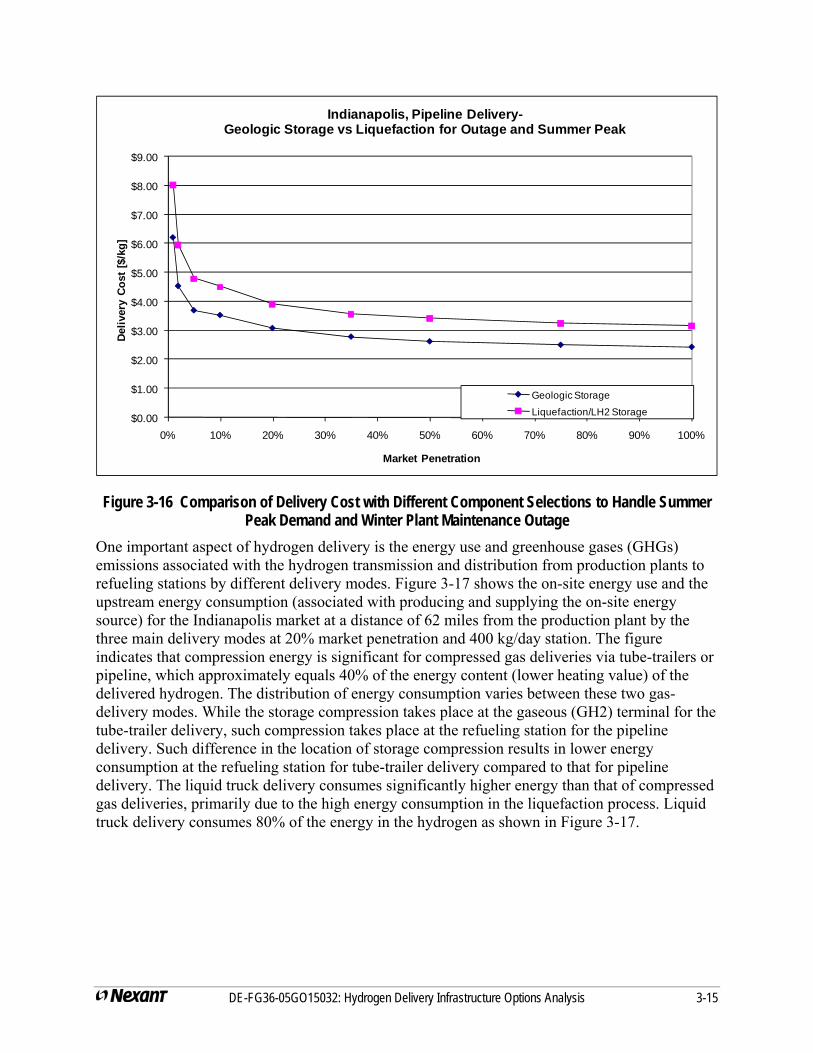
DE-FG36-05GO15032: Hydrogen Delivery Infrastructure Options Analysis 3-15
$0.00
$1.00
$2.00
$3.00
$4.00
$5.00
$6.00
$7.00
$8.00
$9.00
0% 10% 20% 30% 40% 50% 60% 70% 80% 90% 100%
Deliv
ery
Cost
[$/k
g]
Market Penetration
Indianapolis, Pipeline Delivery-Geologic Storage vs Liquefaction for Outage and Summer Peak
Geologic Storage
Liquefaction/LH2 Storage
Figure 3-16 Comparison of Delivery Cost with Different Component Selections to Handle Summer Peak Demand and Winter Plant Maintenance Outage
One important aspect of hydrogen delivery is the energy use and greenhouse gases (GHGs) emissions associated with the hydrogen transmission and distribution from production plants to refueling stations by different delivery modes. Figure 3-17 shows the on-site energy use and the upstream energy consumption (associated with producing and supplying the on-site energsource) for the Indianapolis market at a distance of 62 miles from the production plant by the three main delivery modes at 20% market penetration and 400 kg/day station. The figure indicates that compression energy is significant for compressed gas deliveries via tube-trailers or pipeline, which approximately equals 40% of the energy content (lower heating value) of thdelivered hydrogen. The distribution of energy consumption varies between these two gas-delivery modes. While the storage compression takes place at the gaseous (GH2) terminal for thetube-trailer delivery, such compression takes place at the refueling station for the pipeline delivery. Such difference in the location of storage compression results in lower energy consumption at the refueling station for tube-trailer delivery compared to that for pipeline delivery. The liquid truck delivery consumes significantly higher energy than that of compressed gas deliveries, primarily due to the high energy consumption in the liquefaction process. Liquid truck delivery consumes 80% of the energy in the hydrogen as shown in Figure 3-17.
y
e
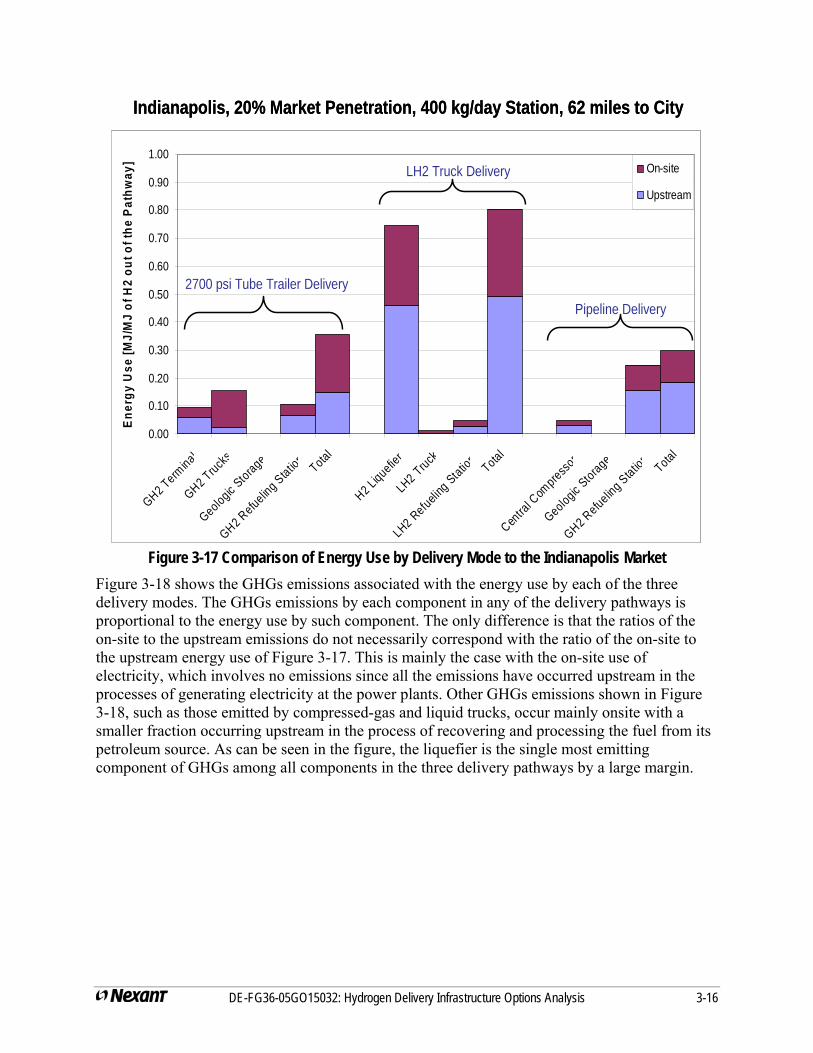
DE-FG36-05GO15032: Hydrogen Delivery Infrastructure Options Analysis 3-16
0.00
0.10
0.20
0.30
0.40
0.50
0.60
0.70
0.80
0.90
1.00
GH2 Terminal
GH2 Trucks
Geologic Storage
GH2 Refueling Station
Total
H2 Liquefie
r
LH2 Truck
LH2 Refueling Statio
nTotal
Centra
l Com
pressor
Geologic Storage
GH2 Refueling Station
Total
Ener
gy U
se [M
J/M
J of
H2
out o
f the
Pat
hway
] On-site
Upstream
Indianapolis, 20% Market Penetration, 400 kg/day Station, 62 miles to City
2700 psi Tube Trailer Delivery
LH2 Truck Delivery
Pipeline Delivery
Figure 3-17 Comparison of Energy Use by Delivery Mode to the Indianapolis Market
Figure 3-18 shows the GHGs emissions associated with the energy use by each of the three delivery modes. The GHGs emissions by each component in any of the delivery pathways is proportional to the energy use by such component. The only difference is that the ratios of the on-site to the upstream emissions do not necessarily correspond with the ratio of the on-site tothe upstream energy use of Figure 3-17. This is mainly the case with the on-site use of electricity, which involves no emissions since all the emissions have occurred upstream in thprocesses of generating electricity at the power plants. Other GHGs emissions shown in Figure 3-18, such as those emitted by compressed-gas and liquid trucks, occur mainly onsite with a smaller fraction occurring upstream in the process of recovering and processing the fuel frompetroleum source. As can be seen in the figure, the liquefier is the single most emitting component of GHGs among all components in the three delivery pathways by a large margin.
e
its
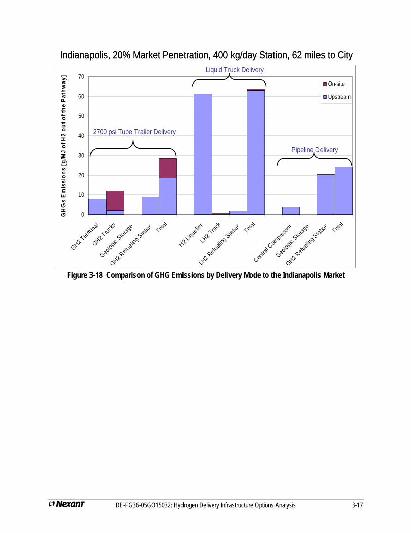
0
10
20
30
40
50
60
70
GH2 Terminal
GH2 Trucks
Geologic Storage
GH2 Refueling Station
Total
H2 Liquefie
r
LH2 Truck
LH2 Refueling Statio
nTotal
Centra
l Com
pressor
Geologic Storage
GH2 Refueling Station
Total
GH
Gs
Emis
sion
s [g
/MJ
of H
2 ou
t of t
he P
athw
ay]
On-site
Upstream
2700 psi Tube Trailer Delivery
Liquid Truck Delivery
Pipeline Delivery
Indianapolis, 20% Market Penetration, 400 kg/day Station, 62 miles to City
Figure 3-18 Comparison of GHG Emissions by Delivery Mode to the Indianapolis Market
DE-FG36-05GO15032: Hydrogen Delivery Infrastructure Options Analysis 3-17
Section 4 Conclusions and Recommendations
The H2A Delivery Scenario Model V2 (HDSAM V2) estimates the delivery cost of hydrogen using current costs of available technologies. The model’s purpose is to identify components with the largest impact on delivery cost and to guide the direction of research for possible delivery cost reductions. The model allows the user to evaluate a broad range of variables in the calculation of hydrogen delivery cost, including:
Urban, rural, or mixed markets
City (or city population)
Hydrogen market penetration
Refueling station capacity
Distance from production plant to the hydrogen market
Delivery method (tube trailer, liquid truck, or gas pipeline)
Storage method for summer peak demand and production plant outages (geologic or liquid)
Refueling station hourly demand profiles.
The results of numerous model runs, over a wide range of market conditions, show the following general conclusions for currently available hydrogen delivery technologies:
At low market demands (<10% market penetration)with a central plant 62 or greater miles from the city, the delivery cost of hydrogen to refueling stations is high for all delivery modes ($5-$10/kg of hydrogen or even higher), suggesting that distributed production of hydrogen at refueling stations may serve the early markets for hydrogen vehicles. Alternatively a small semi-central plant located at the city gate may provide sufficiently low delivery cost by tube trailers.
If the city size is small (<500,000 people), if the market penetration is low (<10%), if the refueling station capacity is small (<400 kg/day), and if the distance to the production plant is modest (<62 miles), then hydrogen delivery by tube trailer is the lowest cost option. For early market conditions, delivery costs of $5 to $12/kg are anticipated.
If one or two market conditions move from the ‘small’ to the ‘large’ category, hydrogen delivery by liquid truck may be the lowest cost approach. However the energy consumed is 80% the energy in the hydrogen delivered due to the energy intensity of hydrogen liquefaction.
For a maturing hydrogen fuel cell vehicle market (>20% market penetration), hydrogen delivery by pipeline is almost universally preferred, with expected delivery costs in the range of $2 to $4/kg of hydrogen depending on the size of the city and market penetration level.
If the hydrogen production plants are located less than 62 miles from the “city gate” and if tube trailers are developed that could deliver about 1,000 kg of hydrogen, the
DE-FG36-05GO15032: Hydrogen Delivery Infrastructure Options Analysis 4-1
cost of tube trailer delivery drops significantly and approaches the cost of pipeline delivery. This approach could avoid the required cost, time, disruption, and potential safety concerns of building hydrogen pipeline distribution systems in urban areas.
The energy use in the delivery of hydrogen can be significant. For pipeline delivery, tube trailer delivery and liquid hydrogen delivery the Well to Vehicle Tank energy use is about 30%, 35% and 80% of the energy in the hydrogen delivered respectively.
Greenhouse gas emissions are the lowest with pipeline delivery, moderately higher with tube trailer delivery, but essentially double with liquid delivery.
The cost of hydrogen delivery is a function of the market demand in terms of kg of hydrogen per square mile (determined by the population density, vehicle ownership rate, and % transportation vehicle market penetration) and the distance between the central manufacturing plant and the market. Thus delivery costs to the vast majority of the U.S.(>75% of the land area) can be reasonably modeled in HDSAM V2 by drawing large enough circles (markets) around each major city and defining the population density as a function of distance from the center of the circle.
There would be sufficient hydrogen demand to justify a central hydrogen production plant (50,000 to 350,000 kg/day of hydrogen production) located near any significant urban area (>300,000 people) even at modest transportation vehicle market penetration (>25%). Large urban areas will require multiple large hydrogen production plants to supply them. As a result of this and the relatively high cost of hydrogen transport, it would be expected to have the production plant(s) located as close the city as permitted. This is likely to be less than 62 miles from the “city gate” and quite possibly at the city’s edge.
For pipeline delivery, low pressure (~2,500 psi) compressed gas storage is required at the refueling station to accommodate the large difference between day and evening refueling demands. The low pressure storage is an adjunct to the nominal 6200 psi cascade system, which is required to fill the vehicles to 5,000 psi.
For tube trailer delivery, the adjunct storage capacity to the cascade system is provided by the tube trailer, which remains at the refueling station. For liquid delivery, the adjunct storage capacity is provided by the liquid tank, in conjunction with a liquid pump and vaporizer.
Refueling station capacities significantly impact the delivery cost of hydrogen for all delivery modes. Increasing refueling station capacity up to 1000 kg/day results in significant delivery cost reduction. Further increase in station capacity results in modest to negligible reduction in cost of delivery. However, it should be noted that as the station capacity increases, the corresponding number of stations would proportionally decrease to satisfy the same demand of a given market, thus affecting the accessibility of refueling stations to hydrogen vehicles in that market if the total market demand is not high enough (e.g. < 20% of the vehicle market during the transition to widespread use of hydrogen fuel cell vehicles). (Note: a 1000 kg/day hydrogen refueling station is about a third the size of the new gasoline stations being built in urban areas.)
DE-FG36-05GO15032: Hydrogen Delivery Infrastructure Options Analysis 4-2
To accommodate production plant outages or the variation in seasonal demand, compressed gas storage in a geologic formation is clearly the preferred approach. However, if such formations are not available along the delivery pathway, liquid storage is the next lowest cost option, followed a distant third by compressed gas storage in steel pressure vessels.
The HDSAM V2 model provides the capital cost and the greenhouse gas emission data to develop recommendations on the preferred delivery infrastructure as the hydrogen economy matures.
Tube trailers, liquid truck delivery, and pipelines are each the optimum delivery method at different points in the maturation of the hydrogen infrastructure. As such, efforts to reduce the energy requirements and the capital cost of each method can reduce the overall cost of delivery in the transition to and widespread use of hydrogen fuel cell vehicles. Possible research efforts include the following:
Lower cost composite based high pressure storage vessels for hydrogen storage and cascade charging systems at the refueling station. These storage vessels are a major cost for all delivery pathways.
Composite based high pressure (7,000 psi) tube trailers or other approaches to a tube trailer with a capacity of 1000 kg of hydrogen.
FRP transmission and or distribution pipelines to reduce pipeline capital and thus pipeline delivery costs. The distribution lines are the larger portion of the pipeline costs.
Magnetic, or other novel, methods for hydrogen liquefaction.
Finally, possible uses and enhancements to HDSAM V2 include:
Examining and improving the research targets for delivery components.
Improving the optimization procedures for calculating the size and location of hydrogen distribution lines within a city.
Adding novel hydrogen carriers to the delivery pathways. Potential carriers include metal hydrides/alanates, chemical hydrides, liquid phase hydrogen carriers, and high surface area sorbents. Preliminary studies indicate the latter two approaches hold some promise for hydrogen delivery.
Adding an option for 10,000 psi vehicle fills
Including, as required, the equipment to pre-cool the hydrogen gas prior to dispensing for 10,000 psi fills and vehicle hydride and sorbent storage approaches.
Combining the H2A Central and the Distributed Production Models with the HDSAM delivery model.
Examining the use of cold (-50oC to -150oC) hydrogen compressed gas for delivery and vehicle storage.
DE-FG36-05GO15032: Hydrogen Delivery Infrastructure Options Analysis 4-3

DE-FG36-05GO15032: Hydrogen Delivery Infrastructure Options Analysis 4-4
Adding regional effects to the model, such as local labor rates, or the difference between the North and the South in the seasonal variation in fuel demand (i.e., winter demand in the North is 70 percent of the summer demand, while winter demand in the South is 90 percent of the summer demand)
Incorporating performance and cost data on all hydrogen delivery technologies as they are advanced to lower cost and more efficient systems.