guidance and control of a naval cruise missile572778/fulltext01.pdf · guidance and control of a...
TRANSCRIPT
Guidance and Control of a Naval CruiseMissile
DAMIEN LE VOYER
Masters’ Degree ProjectStockholm, Sweden June 2008
XR-EE-RT 2008:014

Abstract Today the armed forces of many countries need to strike accurately potential enemies, wherever they might be, from a safe place. Since naval units can be deployed almost everywhere in the open sea, the idea of a naval cruise missile emerged in the 70’s. These missiles are designed to be launched from various naval vehicles such as frigates or submarines and strike deeply in the enemy territory. A program called Missile de Croisière Naval (MdCN Naval Cruise Missile) was therefore launched in 2006 by the DGA, the French procurement agency. MBDA is the industrial company appointed by the DGA to design and build the missile. Control aspects on a cruise missile are of primary interest since they impact the reliability, performance and availability of the weapon. In the aeronautics and weapon industry, gain scheduled controllers are used in most cases. However, many non-linear techniques have been developed in the literature and might improve the behaviour of the missile. The main objective of the present thesis is to apply non-linear techniques on the control and guidance loops of the MdCN too see whether of not they can improve such a system. Based on this report it should be easy for the engineers of the DGA to compare the controllers of the thesis and the classical gain scheduled controllers used in the industry. To achieve this task some basic knowledge of flight dynamics are recalled and a model of the MdCN is computed and divided into the control loop and the guidance loop. Then a non-linear controller for the launch phase using a Lyapunov based technique called back-stepping is designed and tested through a statistic analysis. During the cruise phase different anti-windup strategies are applied on the propulsion control loop of the missile and compared. Finally a software interface with a navigation-dedicated tool is coded and implemented in Simulink to analyse the complete Guidance-Navigation-Control loop and to see how navigation errors impact the control algorithms. The main contributions of this thesis are the controllers designed for the launch phase and the propulsion loop that will be compared with the controller that MBDA is going to deliver next year to see whether or not the non-linear techniques used in the thesis should be used on the missile. Furthermore, all the tools and procedure set up to interface the control and guidance laws with the navigation models and filters will give the possibility to the DGA to have a deeper understanding of the algorithms used by MBDA and to make sure that navigation and estimation issues are properly taken in account when designing the control and guidance laws.

Acknowledgements This thesis was held at the LRBA in Vernon. I would like to thanks all my colleagues, at the LRBA for the nice moments we shared together in a nice work atmosphere during my stay in Vernon. Special thanks for my supervisor, Florent Le Bras for providing me the opportunity to join the project, who together with the people of PSM and SysNav among others: Loic Banlin, Laurent Burlion, Fabien Debaye, The Truyen Mai, Thierry Marot, Jean Pierre Nouailles, Fabien Petit and Olivier Tabart have shared their knowledge, expertise and support and who provided an always nice but challenging environment. I hope for the best concerning the future of the centre. I also would like to thank Professor Elling Jacobsen, for keeping me motivated during the thesis and for supervising my work from Sweden for KTH. Finally, a special thanks to my family for the help and support given during this six months. Thank you.

Contents Abstract ...................................................................................................................................... 2 Acknowledgements .................................................................................................................... 4 Introduction ................................................................................................................................ 8 I. Context of the thesis ............................................................................................................... 9
I.1 Presentation of the Délégation Générale pour l’Armement .............................................. 9 I.1.a The Délégation Générale pour l’Armement ............................................................... 9 I.1.b Laboratoire de Recherches Balistiques et Aérodynamiques .................................... 10 I.1.c Performance de Systèmes Missiles .......................................................................... 11
I.2 Presentation of the Missile de Croisière Naval ............................................................... 11 I.2.a Context ..................................................................................................................... 11 I.2.b General characteristics of the missile ...................................................................... 12 I.2.c Chronology of a launch ............................................................................................ 13
II. Modelling of the missile ...................................................................................................... 14 II.1 Aerodynamics Basis ...................................................................................................... 15
II .1.a General reference systems ..................................................................................... 15 II .1.b Aerodynamic model .............................................................................................. 22
II.2 Mass and inertia of the system missile+booster ............................................................ 23 II.3 Expression of the booster’s Thrust ................................................................................ 25 II.4 Nozzles actuators and limitations .................................................................................. 27 II.5 State space model .......................................................................................................... 28
II.5.a Notations ................................................................................................................. 28 II.5.b Force equation ........................................................................................................ 29 II.5.c Torque equation ...................................................................................................... 29 II.5.d Model simplification ............................................................................................... 30 II.5.e State space and guidance piloting decoupling ........................................................ 31
III. Launch phase ...................................................................................................................... 33 III.1 Problematic of the launch phase. .................................................................................. 33 III.2 First controller design ................................................................................................... 33
III.2.a The backstepping theory ........................................................................................ 34 III.2.b Quaternions ........................................................................................................... 34 III.2.c State space transformation ..................................................................................... 35 III.2.d Backstepping design .............................................................................................. 36 III.2.e Booster control ...................................................................................................... 37 III.2.f First results ............................................................................................................. 38
III.3 Controller improvement ............................................................................................... 40 III.3.a New control sequence ............................................................................................ 40 III.3.b Angle of Attack and Sideslip reduction ................................................................ 41 III.3.c Statistic optimisation ............................................................................................. 42
III.4 Performance analysis .................................................................................................... 48 III.4.a Multi-azimuth launch ............................................................................................ 48 III.4.b Carrier velocity influence ...................................................................................... 50 III.4.c Wind influence ...................................................................................................... 51 III.4.d Conclusion ............................................................................................................. 52
IV. Cruise phase ....................................................................................................................... 52 IV.1 Control Strategy ........................................................................................................... 52 IV.2 Guidance ...................................................................................................................... 52
IV.2.a Mid-flight guidance ............................................................................................... 52 IV.2.b Altitude Control .................................................................................................... 54
IV.3 Three-loop autopilot ..................................................................................................... 54
IV.4 Propulsion loop ............................................................................................................ 54 IV.4.a Anti-windup .......................................................................................................... 54 IV.4.b Application on the propulsion control loop .......................................................... 56 IV.4.c Case study ............................................................................................................. 57
IV.5 Results .......................................................................................................................... 58 V. Navigation issues ................................................................................................................. 60
V.1 Interface with Oceani .................................................................................................... 60 V.2 Kinematics model and numerical integration ................................................................ 61 V.3 Inertial Navigation System simulation .......................................................................... 64
Conclusion ................................................................................................................................ 65 Summary .............................................................................................................................. 65 Future works ......................................................................................................................... 66
Appendix A: A3 ....................................................................................................................... 67 A.1 Presentation of A3 ......................................................................................................... 67 A.2 Implementation of the model under A3 ........................................................................ 70
A.2.a Launch chronology ................................................................................................. 70 A.2.b A3 Model architecture ............................................................................................ 70
Appendix B: S4 ........................................................................................................................ 73 B.1. FlightGear interface ...................................................................................................... 73 B.2.Stage .............................................................................................................................. 74
Appendix C: Three loops autopilot .......................................................................................... 75 C.1 Transfer functions calculation ....................................................................................... 75 C.2 Controller design ........................................................................................................... 76
Figure table ............................................................................................................................... 79 Bibliography ............................................................................................................................. 81
Introduction Today the armed forces of many countries need to strike accurately from a safe place potential enemies wherever they might be. Since naval units can be deployed almost everywhere in the open sea, the idea of a naval cruise missile emerged in the 70’s. These missiles are designed to be launched from various naval vehicles such as frigates or submarines and strike deeply in the enemy territory. This solution was indeed a good answer to the challenge that many countries are facing. However the launch from a naval carrier is much more complicated than the launch from an aircraft or a ground station. First of all since the carrier might be in patrol in an hostile environment, his position, i.e. the initial position of the missile might be subject to uncertainties, due to GPS jamming for example. Furthermore naval missiles are launch from a more or less vertical position without any initial vertical velocity. So during the same phase they need to accelerate enough to start the turbojet propeller, swing up to a horizontal position and reach their cruise trajectory and of course they shouldn’t be a hazard for their carrier! The main goal of this thesis will be to investigate how non-linear techniques might improve the performance and availability of such weapons. A non-linear controller for the launch phase will be designed and tested. In addition to this study some anti-windup techniques are compared and tested on the propulsion loop. And finally an interface between a navigation software, called Oceani and Matlab/Simulink is designed to investigate navigation issues and their influence on the controller. The thesis outlines as follow:
• Chapter I introduces the context of the thesis with a brief presentation of the Direction Générale pour l’Armement and a description of the missile.
• Chapter II presents some basic knowledge in aerodynamics that is then used to derive a model of the missile and its booster.
• Chapter III describes the design of the non-linear controller for the launch phase • Chapter IV deals with the cruise phase, it describes the control-guidance strategy but
emphasis on the anti-windup techniques and the propulsion loop. • Chapter V introduces the navigation issues and the interface designed between Oceani
and Simulink and the influence of navigation errors on the control loops. • Appendix A describes the toolbox used to model the missile under Simulink and all
the implementation issues on the simulator. • Appendix B presents the so-called three-loops autopilot, a classical linear controller
widely used in the industry that will be used here during the cruise phase.
I. Context of the thesis
I.1 Presentation of the Délégation Générale pour l’Armement
I.1.a The Délégation Générale pour l’Armement Founded in 1961 by General De Gaulle the DGA (Direction Générale pour l’Armement) is the French procurement agency. Defence system architect and technical expert serving the Armed Forces, the DGA controls the design and development of weapons systems, and monitors the availability of the necessary industrial and technological capacities. It works closely with military staff from identification of future needs through to user satisfaction. The DGA has three main missions:
• Preparing the future of defence systems • Equipping the armed forces • Promoting defence equipment export
The DGA employs 18 000, of which 80% civilians and 20% military, in many different establishments on the French territory but it has also representations in 20 countries all over the world. The DGA is divided in several directorates. This project will take place in one of them: the Direction de l’Expertise Technique (DET Direction of the technical expertise). The DET consists of several entities among them the technical centres and especially the LRBA.
Minister of Defense
DGA
DET
LRBA
I.1.b Laboratoire de Recherches Balistiques et
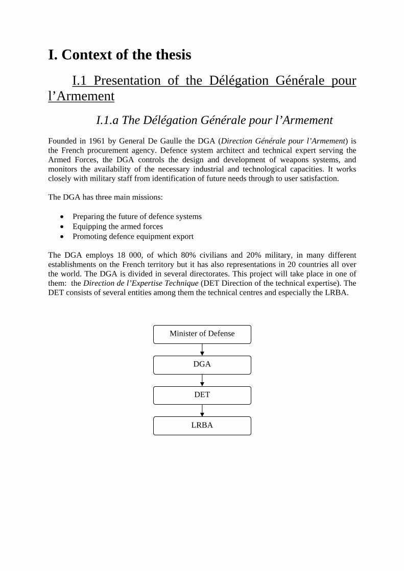
Aérodynamiques The Laboratoire de Recherches Balistiques et Aérodynamiques (LRBA technical centre for research in ballistic and aerodynamics) is one of the technical centres of the DET. Installed on a field of 545 ha, the LRBA is located near the city of Vernon on a plateau above the Seine about 50 minutes North West from Paris.
Figure 1 Air Picture of the LRBA
Since the 1950’s it provides a strong expertise in missile systems and in many armament programs, a brief history of the site is shown below:
• 1928: First mortars ammunition factory
• 17th may 1946: LRBA's foundation, expertise centre on missiles and rockets based on the German knowledge of that time.
• 1946-1970: Many activities in several fields of study: studies on the inertial systems
built by the industry, observation satellites, several ballistic works from 1958, studies on ergol propulsion, rockets trajectories: design of the first French rockets VERONIQUE (1952), VESTA (1964) propellers VEXIN (1963) and VALOIS (1966) which will be used on the space rockets DIAMANT. One of them launched the first French satellite Astérix on 26th November 1965.
• 1971: Transfer of the propulsion activities to the European Propulsion Company
(SNECMA). Military activities in LRBA became a part of the missiles directorate • 1973: LRBA is entrusted with an interdirectorate mission for inertial techniques and
navigation systems. • 1985: Mission for the standardization of environmental tests and techniques.
• 1993: GPS interdirectorate technical centre.
• 2004: Incorporation to DET (Directorate of Technical Expertise)
I.1.c Performance de Systèmes Missiles The LRBA consists in several divisions and departments, the thesis will be held in a department called PSM (Performances de Systèmes Missiles, Performances of Missiles Systems) of the MAN division (Missiles et Armes Nucléaires, Missiles and Nuclear Weapons). The PSMD department provides a technical expertise of the global performances of the Missiles systems from the planning of the mission to the integration of the weapon systems into a bigger one. Generally speaking the work consists of:
• Leading performances studies • Evaluations through numerical simulations • Specifications and needs of weapons systems • Analysis of the technical documentations of the armaments programs • Technical support during negotiations with the industry • Proposition of early studies subjects.
I.2 Presentation of the Missile de Croisière Naval
I.2.a Context During the First Gulf War 1991 the US Army used massively the Tomahawk to strike deeply in the enemy territory. The French Forces realized at that time the benefit they could get from such a cruise missile able to hit any objective in the depth from a safe area by night or by day whatever the weather. To match this need and guarantee its independence toward the US technology, France decided in 1993 to develop its own tactical cruise missiles launched from aircrafts, ships or submarines. A first air-ground anti runway missile called APACHE was designed by Matra Defence (MBDA France today) and is operational in the French Air force since 2002. Based on the work done on the APACHE Matra developed together with British Aerospace another air-ground missile dedicated to the destruction of military or logistic infrastructures. This missile called SCALP-EG in France and Storm Shadow in the United Kingdom was used with success in operation for the first time by the British army in Iraq during the Second Gulf War; the missile is also a commercial success since it has been sold to many countries like Italy, Greece or the United Arab Emirates. Concerning the naval version of the missile called Naval SCALP or MdCN (Missile de Croisière Naval Naval Cruise Missile) the first preliminary studies started in 2002 and are leaded by the DGA while MBDA is the industrial in charge of the program. The department PSM from the LRBA is responsible for the evaluation of the global performances of the
missile that includes the performances of the control laws of the guidance and autopilot devices.
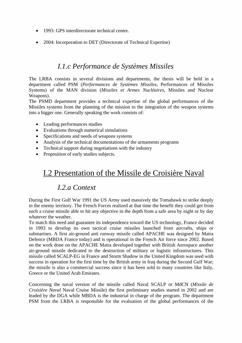
I.2.b General characteristics of the missile The MdCN is to be launched by the future FREMM (multi missions European frigate) and the future submarines SNA/SSN from the class Barracuda. The main components of the missile are:
• Large wingspan wings: for high range and thin airframe. • Turbojet propeller TR 50: This guarantees a good kilometric consumption. • Spreadable wings, deflectors and air entry: To store the missile in NATO standard
tubes of 533mm. The wings, deflector and air entry spread once the missile has been fired and has left his launch device.
• Booster: called SAB (Système d’Accélération et de Basculement acceleration and « tip over » system) is a solid propellant rocket motor with two swivelling nozzles. Since the MdCN is launch from a vertical position, it needs an initial propeller to leave its carrier and move up to a horizontal position where the booster is dropped and the turbojet turned on.
Figure 2 MdCN prototype with its SAB at the bottom
Note the two swivelling nozzles
• DCM (Dispositif de Changement de Milieu Environment change device) : Submarine
version only. The DCM is the waterproof device used to protect the missile when the MdCN is launched from a submarine and has to go from the water into the air. The DCM is dropped as soon as the Missile has left the water.
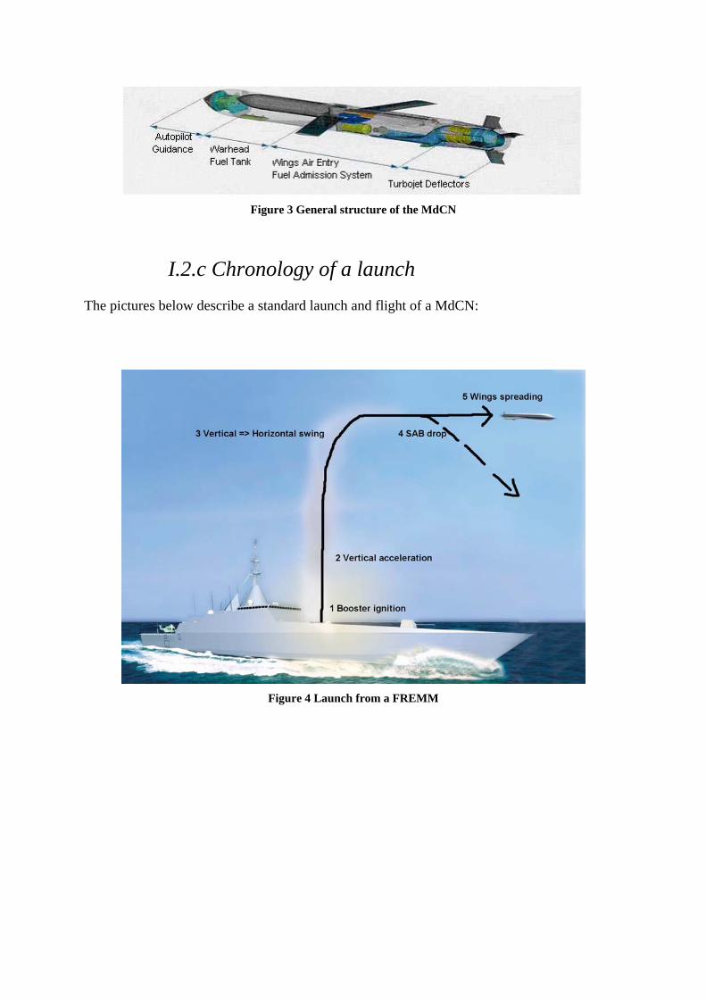
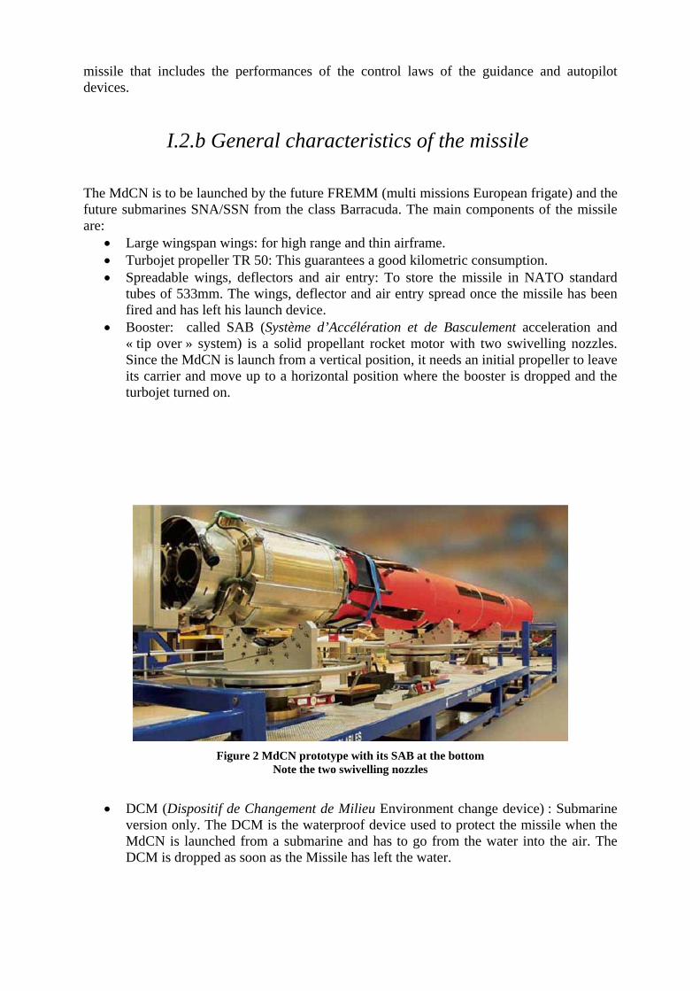
Figure 3 General structure of the MdCN
I.2.c Chronology of a launch The pictures below describe a standard launch and flight of a MdCN:
Figure 4 Launch from a FREMM

Figure 5 Launch from a submarine
II. Modelling of the missile The purpose of this chapter is to derive a model for the missile, i.e. to get a state space model of the system. This model will be derived using a physical modelling based on Newton’s laws. The forces and torques applied on the system are:
The aerodynamic forces The mass and inertial torques The thrust produced by the SAB, the booster of the missile.
In part II.1 the reference systems where this forces and torques are expressed are presented, introducing all the angles used to describe the position and attitude of the missile during a flight. Then the usual model of the aerodynamic force is presented and the aerodynamic coefficients are briefly discussed. Part II.2 deals with the mass and inertial effects. Since the booster is burning some propellant it will loose some weight thus the mass, inertial matrix and center of mass of the missile will evolve with time. The purpose of this part is to describe this evolution. Part II.3 and II.4 deal with the thrust produced by the SAB during the flight. In part II.3 the thrust is derived and then expressed in a proper reference frame (the body reference system
see II.1.a) while part II.4 models the actuators (here the swivelling nozzles) and their limitations. Finally part II.5 presents the state space model obtained after some simplifications. The separation between the slow and fast dynamics is discussed introducing the guidance/control separation.
II.1 Aerodynamics Basis This part presents some general knowledge on aerodynamics that will be useful for the modeling of the missile. For further details on aerodynamics and flight dynamics see [1]
II .1.a General reference systems In this part the reference systems used to express the different vectors (speed, acceleration, forces, torques…) needed to compute a state space model for the missile. Three main reference frames are used:
The earth reference frame with origin G, the centre of mass of the missile and axis linked to the earth. The frame is used as a reference for the attitude of the missile.
The body reference frame with origin G and axis linked to the missile. The angles that describe the rotation from the earth reference to the body reference frame are called Euler angles or attitude angles.
The aerodynamics reference frame with origin G and axis linked to the velocity of the missile. This reference frame is convenient to compute the aerodynamic coefficient of the missile and describe the behaviour of the airflow on the body of the missile.
One can note that all this reference frames are not constants since they depend on the position of G so one can also use a last reference frame called local reference frame which is basically an earth reference system except that it has its origin constant in the initial position of G for example.
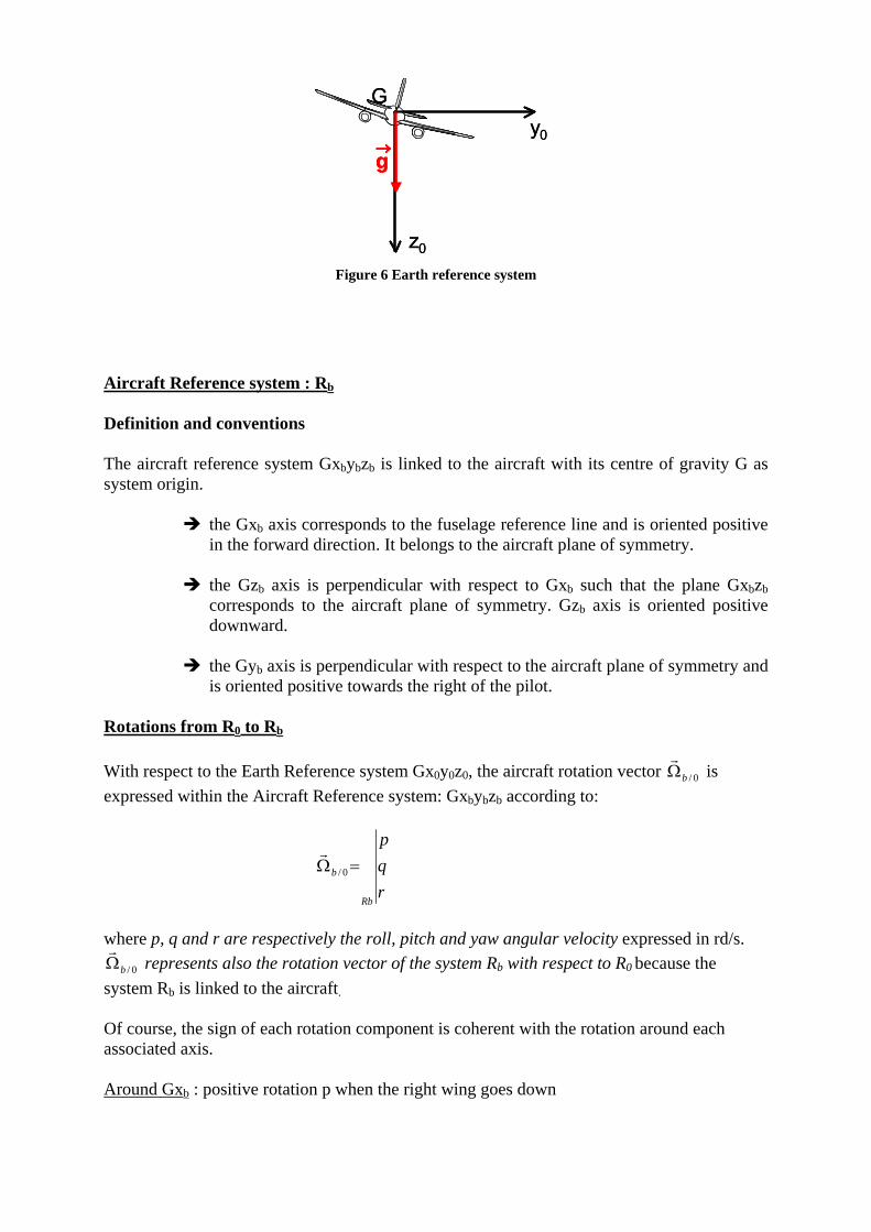
Earth Reference system : R0 The Gz0 axis corresponds to the local vertical line that passes through the aircraft centre of gravity, G. It is oriented positive downward and corresponds to the direction of the gravitation force m. gr seen by the aircraft, see figure 6. The Gx0y0 plane is the local horizontal plane that passes through the aircraft centre of gravity, G. It is usual to take, for Gx0 direction, the geographic or magnetic Earth North.
y0
G
z0
→g
y0
G
z0
→g→→g
Figure 6 Earth reference system
Aircraft Reference system : Rb Definition and conventions The aircraft reference system Gxbybzb is linked to the aircraft with its centre of gravity G as system origin.
the Gxb axis corresponds to the fuselage reference line and is oriented positive in the forward direction. It belongs to the aircraft plane of symmetry.
the Gzb axis is perpendicular with respect to Gxb such that the plane Gxbzb corresponds to the aircraft plane of symmetry. Gzb axis is oriented positive downward.
the Gyb axis is perpendicular with respect to the aircraft plane of symmetry and is oriented positive towards the right of the pilot.
Rotations from R0 to Rb With respect to the Earth Reference system Gx0y0z0, the aircraft rotation vector 0/bΩ
r is
expressed within the Aircraft Reference system: Gxbybzb according to:
rqp
Rb
b =Ω 0/
r
where p, q and r are respectively the roll, pitch and yaw angular velocity expressed in rd/s.
0/bΩr
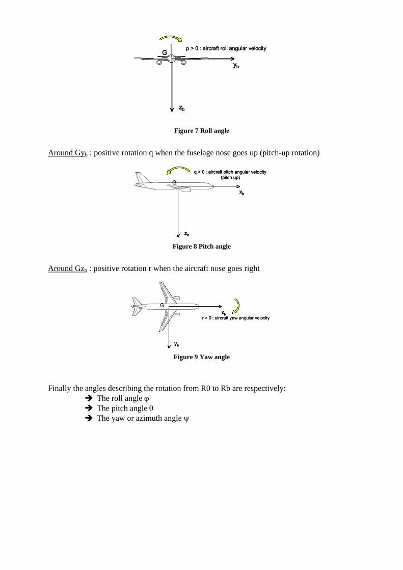
represents also the rotation vector of the system Rb with respect to R0 because the system Rb is linked to the aircraft. Of course, the sign of each rotation component is coherent with the rotation around each associated axis. Around Gxb : positive rotation p when the right wing goes down
yb
G
zb
p > 0 : aircraft roll angular velocity
yb
G
zb
yb
G
zb
p > 0 : aircraft roll angular velocity
Figure 7 Roll angle
Around Gyb : positive rotation q when the fuselage nose goes up (pitch-up rotation)
q > 0 : aircraft pitch angular velocity(pitch up)
xb
G
zb
q > 0 : aircraft pitch angular velocity(pitch up)
xb
G
zb
xb
G
zb Figure 8 Pitch angle
Around Gzb : positive rotation r when the aircraft nose goes right
Gxb
yb
r > 0 : aircraft yaw angular velocity
Gxb
yb
Gxb
yb
r > 0 : aircraft yaw angular velocity
Figure 9 Yaw angle
Finally the angles describing the rotation from R0 to Rb are respectively:
The roll angle ϕ The pitch angle θ The yaw or azimuth angle ψ
zb
xb
yb
z0
x0
y0
ψxψ
θ
yψ
ψ
ψ
θ
φ
φ
ψ azimuth angleθ pitch attitudeφ bank angle
G
horizontal plane
vertical plane containing the fuselage axis xb
zθ
θφ
zb
xb
yb
z0
x0
y0
ψxψ
θ
yψ
ψ
ψ
θ
φ
φ
ψ azimuth angleθ pitch attitudeφ bank angle
G
horizontal plane
vertical plane containing the fuselage axis xb
zθ
θφ
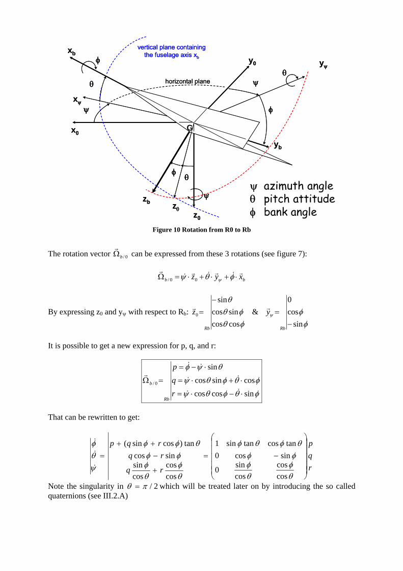
Figure 10 Rotation from R0 to Rb
The rotation vector 0/bΩ
r can be expressed from these 3 rotations (see figure 7):
bb xyz r&r&r&
r⋅+⋅+⋅=Ω φθψ ψ00/
By expressing z0 and yψ with respect to Rb: φ
φφθφθ
θ
ψ
sincos0
&coscossincos
sin
0
−=
−=
RbRb
yz rr
It is possible to get a new expression for p, q, and r:
φθφθψ
φθφθψ
θψφ
sincoscos
cossincos
sin
0/
⋅−⋅=
⋅+⋅=
⋅−=
=Ω&&
&&
&&r
rq
p
Rb
b
That can be rewritten to get:
rqp
rq
rqrqp
⎟⎟⎟⎟⎟
⎠
⎞
⎜⎜⎜⎜⎜
⎝
⎛
−=
+
−++
=
θφ
θφ
φφθφθφ
θφ
θφ
φφθφφ
ψθφ
coscos
cossin0
sincos0tancostansin1
coscos
cossin
sincostan)cossin(
&
&
&
Note the singularity in 2/πθ = which will be treated later on by introducing the so called quaternions (see III.2.A)
Of course, the sign of each rotation component is coherent with the rotation around each associated axis. By convention we assume:
πφπ
πθππψπ
<<−
≤≤−
<<−
22 (1)
From these three angles one can compute the rotation matrix from R0 to Rb which is useful to change reference frame. Let 0X and bX be the expression of the vector X in R0 and Rb respectively then:
bXbX ):0(0 ℜ= (2)
Actually ):0( bℜ is the product of three rotations, thus:
( )⎟⎟⎟
⎠
⎞
⎜⎜⎜
⎝
⎛−
⎟⎟⎟
⎠
⎞
⎜⎜⎜
⎝
⎛
−⎟⎟⎟
⎠
⎞
⎜⎜⎜
⎝
⎛ −=ℜ
ϕϕϕϕ
θθ
θθψψψψ
cossin0sincos0001
cos0sin010
sin0cos
1000cossin0sincos
:0 b (3)
( )⎟⎟⎟
⎠
⎞
⎜⎜⎜
⎝
⎛
−++−
−=ℜ
φθψφψφθψφψφθφθψφψφθψφψφθ
θψθψθ
coscoscossinsincossinsinsincoscossinsincoscoscossinsinsinsincoscossinsin
sinsincoscoscos:0 b (4)
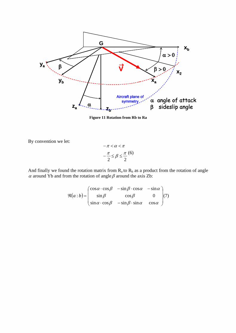
Aerodynamic Reference system : Ra Definition and conventions The aircraft reference system Gxayaza is linked to the aircraft velocity vector V
r.
The Gxa axis corresponds to the aircraft velocity V
rdirection and is oriented positive in the
same direction. The Gza axis is perpendicular with respect to Gxa and located within the aircraft plane of symmetry Gxbzb ; Gza axis is oriented positive downward. The Gya axis completes the Aerodynamic Reference system Ra.
The expression of V with respect to Ra and Rb is: βα
ββα
cossinsin
coscos
00
⋅⋅⋅
==VVVV
V
RbRa
r(5)
Rotations from Rb to Ra
α angle of attackβ sideslip angle
xb
xa
α > 0
x2
α
β β > 0
zbza
yb
ya
G
→V
Aircraft plane of symmetry α angle of attack
β sideslip angle
xb
xa
α > 0
x2
α
β β > 0
zbza
yb
ya
G
→V→→V
Aircraft plane of symmetry
Figure 11 Rotation from Rb to Ra
By convention we let:
22πβπ
παπ
≤≤−
<<−(6)
And finally we found the rotation matrix from Ra to Rb as a product from the rotation of angle α around Yb and from the rotation of angle β around the axis Zb:
( )⎟⎟⎟
⎠
⎞
⎜⎜⎜
⎝
⎛
⋅−⋅
−⋅−⋅=ℜ
ααββαββ
ααββα
cossinsincossin0cossin
sincossincoscos: ba (7)
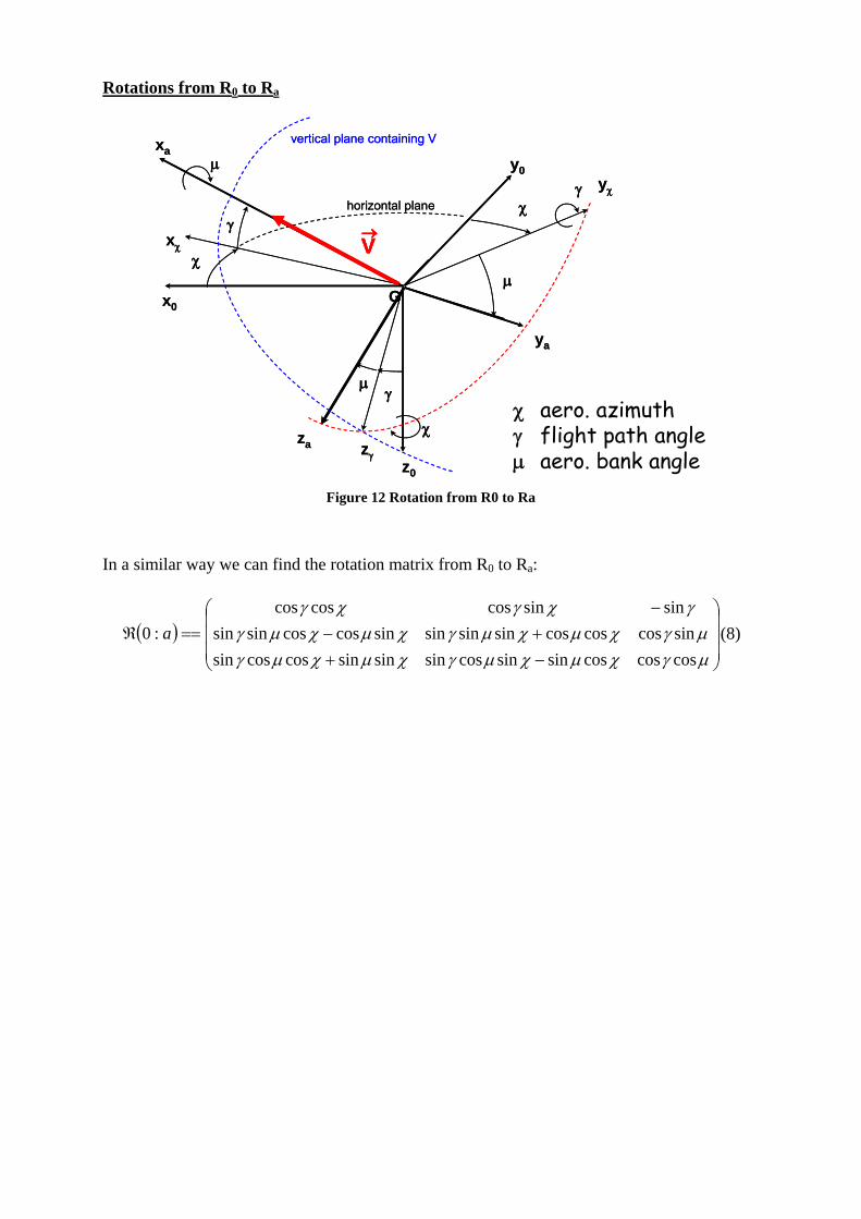
Rotations from R0 to Ra
za
xa
ya
z0
x0
y0
χxχ
γ
yχ
χ
χ
γ
μ
μ
χ aero. azimuthγ flight path angleμ aero. bank angle
G
horizontal plane
vertical plane containing V
zγ
γμ
→V
za
xa
ya
z0
x0
y0
χxχ
γ
yχ
χ
χ
γ
μ
μ
χ aero. azimuthγ flight path angleμ aero. bank angle
G
horizontal plane
vertical plane containing V
zγ
γμ
→V→→V
Figure 12 Rotation from R0 to Ra
In a similar way we can find the rotation matrix from R0 to Ra:
( )⎟⎟⎟
⎠
⎞
⎜⎜⎜
⎝
⎛
−++−
−==ℜ
μγχμχμγχμχμγμγχμχμγχμχμγ
γχγχγ
coscoscossinsincossinsinsincoscossinsincoscoscossinsinsinsincoscossinsin
sinsincoscoscos:0 a (8)
II .1.b Aerodynamic model Definition and conventions
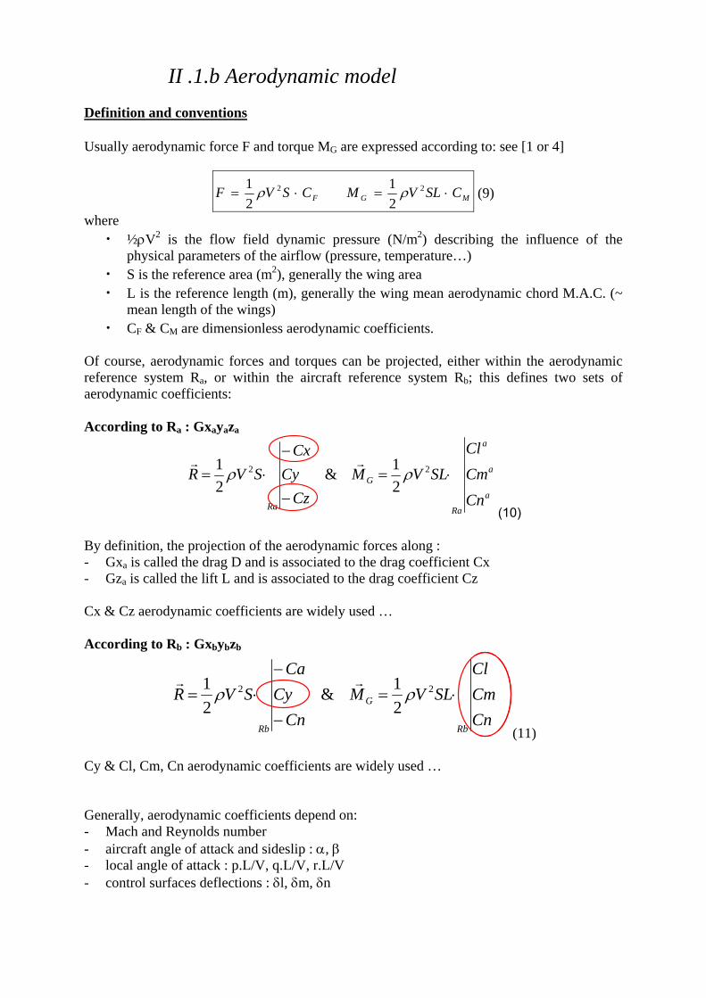
Usually aerodynamic force F and torque MG are expressed according to: see [1 or 4]
MGF CSLVMCSVF ⋅=⋅= 22
21
21 ρρ (9)
where • ½ρV2 is the flow field dynamic pressure (N/m2) describing the influence of the
physical parameters of the airflow (pressure, temperature…) • S is the reference area (m2), generally the wing area • L is the reference length (m), generally the wing mean aerodynamic chord M.A.C. (~
mean length of the wings) • CF & CM are dimensionless aerodynamic coefficients.
Of course, aerodynamic forces and torques can be projected, either within the aerodynamic reference system Ra, or within the aircraft reference system Rb; this defines two sets of aerodynamic coefficients: According to Ra : Gxayaza
a
a
a
Ra
G
Ra CnCmCl
SLVMCz
CyCx
SVR ⋅=−
−⋅= 22
21&
21 ρρ
rr
a
a
a
Ra
G
Ra CnCmCl
SLVMCz
CyCx
SVR ⋅=−
−⋅= 22
21&
21 ρρ
rr
(10)
By definition, the projection of the aerodynamic forces along : - Gxa is called the drag D and is associated to the drag coefficient Cx - Gza is called the lift L and is associated to the drag coefficient Cz Cx & Cz aerodynamic coefficients are widely used … According to Rb : Gxbybzb
CnCmCl
SLVMCn
CyCa
SVR
Rb
G
Rb
⋅=−
−⋅= 22
21&
21 ρρ
rr
CnCmCl
SLVMCn
CyCa
SVR
Rb
G
Rb
⋅=−
−⋅= 22
21&
21 ρρ
rr
(11) Cy & Cl, Cm, Cn aerodynamic coefficients are widely used … Generally, aerodynamic coefficients depend on: - Mach and Reynolds number - aircraft angle of attack and sideslip : α, β - local angle of attack : p.L/V, q.L/V, r.L/V - control surfaces deflections : δl, δm, δn
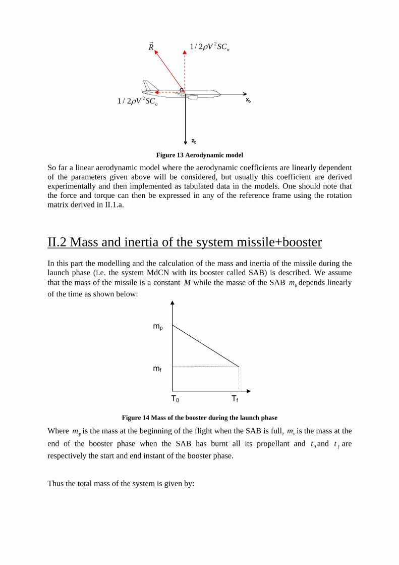
Figure 13 Aerodynamic model
So far a linear aerodynamic model where the aerodynamic coefficients are linearly dependent of the parameters given above will be considered, but usually this coefficient are derived experimentally and then implemented as tabulated data in the models. One should note that the force and torque can then be expressed in any of the reference frame using the rotation matrix derived in II.1.a.
II.2 Mass and inertia of the system missile+booster In this part the modelling and the calculation of the mass and inertia of the missile during the launch phase (i.e. the system MdCN with its booster called SAB) is described. We assume that the mass of the missile is a constant M while the masse of the SAB bm depends linearly of the time as shown below:
Figure 14 Mass of the booster during the launch phase
Where pm is the mass at the beginning of the flight when the SAB is full, vm is the mass at the end of the booster phase when the SAB has burnt all its propellant and 0t and ft are respectively the start and end instant of the booster phase. Thus the total mass of the system is given by:
T0 Tf
mf
mp
q > 0 : aircraft pitch angular velocity(pitch up)
xb
G
zb
q > 0 : aircraft pitch angular velocity(pitch up)
xb
G
zb
xb
G
zb
aSCV 22/1 ρ
nSCV 22/1 ρRr
)()()( 00
ttttmm
MtmMtMf
pvbt −
−
−+=+= (12)
To compute the matrix of inertia of the system we will assume that the missile is a perfect cylinder of constant density and the SAB a punctual mass applied at the bottom of the cylinder in the point B. Let L be the total length of the missile and R its radius. The inertia matrix of the system without SAB in 0G the centre of gravity of the cylinder is given by:
⎟⎟⎟⎟⎟⎟⎟
⎠
⎞
⎜⎜⎜⎜⎜⎜⎜
⎝
⎛
+
+=
)124
(00
0)124
(0
002
22
22
2
0
LRM
LRM
MR
IG (13)
Adding the SAB we have:
⎟⎟⎟⎟⎟⎟⎟
⎠
⎞
⎜⎜⎜⎜⎜⎜⎜
⎝
⎛
++
++=
4)()
124(00
04
)()124
(0
002
222
222
2
0
LtmLRM
LtmLRM
MR
I
b
bG(14)
L
R
G0 x
G x
PL x PR x B x
X
x
y z

Finally according to the parallel axis theorem1 the inertia matrix in G the centre of gravity of the whole system is given by:
⎟⎟⎟
⎠
⎞
⎜⎜⎜
⎝
⎛
++=2
0
20
20
0
000000
))((GzG
GyGGxG
tmMII bGG (15)
⎟⎟⎟⎟⎟⎟⎟
⎠
⎞
⎜⎜⎜⎜⎜⎜⎜
⎝
⎛
++++
++++=
))(
)(1(
4)()
124(00
0))(
)(1(
4)()
124(0
002
222
222
2
MtmtmLtmLRM
MtmtmLtmLRM
MR
I
b
bb
b
bbG
(16)
Note: The position of the centre of gravity of the whole system is given by:
00
2/
)()(
)()(
00
L
Mtmtm
BGMtm
tmGG
b
b
b
b
−
+=
+= (17)
II.3 Expression of the booster’s Thrust The SAB is a solid propellant rocket motor. The norm of the thrust produced by the SAB therefore can’t be controlled and follow the profile shown on the left. In a first approximation we will consider that after the ignition the thrust follows a perfect step to Fp.
1 According to the parallel axis if the axis of rotation is displaced by a vector R = (a b c)t from the centre of mass,
the new moment of inertia equals ⎟⎟⎟
⎠
⎞
⎜⎜⎜
⎝
⎛
++
++=
22
22
22
babcacbccaabacabcb
MII oldnew with the M the total
mass of the system studied
T0 Tf
ΔFFp
The missile can however be controlled since the nozzles can rotate around the axis Y and Z. Indeed a deflection of the same angle Yδ around the Y axis of the two nozzles will create a pitch; a deflection of the angle Zδ around the Z axis of the two nozzles will create a yaw and a different deflection of the nozzles around the Y axis will create a roll. Thus it is possible to control the torque produced by the nozzles and to guide the missile in the good direction.
The expression of the force produced by the two swivelling nozzles is here expressed in the body reference system. The nozzles rotate around the axis Y and Z of the body frame so using two rotation one can express the thrust in the body frame. Hence the thrust is given by:
00
cossinsincossin0cossin
sinsincoscoscos F
YZYZYZZ
YZYZYpF b
⎟⎟⎟
⎠
⎞
⎜⎜⎜
⎝
⎛−
−=
δδδδδδδ
δδδδδr (18)
Thus
00),(Pr
FZrXrPpF bb
r δδ=r
and
00),(F
ZlXlPpF bPl
bl δδ=
r
where bPPr and bPlP will be the rotation matrix
from the “thrust axis” to the body axis system respectively for the right and left nozzle.
Assume that the force created by the nozzle is applied on the missile in the point rP for the right nozzle and in the point lP for the left one.
Since these force are not applied directly on the centre of mass G of the whole system they create the following torque around G (see figure on the left) given by the moment arm formula:
0
))(
)(1(2/
00),(Pr e
Mtmtm
LFZrXrPGPFpM
b
b
br
br
br
+−
∧=∧= δδr
Y
δYl δZl
X
Z
Fl
δYr
δZr
F
G
Pl
x
Pr
L
FpR FpL
G0 x
G x
PL x PR x B x
e
X
x
y z
Mp
(19) for the right nozzle
0
))(
)(1(2/
00),( e
Mtmtm
LFZlXlPGPFpM
b
b
bPll
bl
bl −
+−
∧=∧= δδr
(20) for the left nozzle
II.4 Nozzles actuators and limitations
The nozzles actuators are to be designed but they will have to answer to a step with a rise time, without overshoot, equal or smaller than the rise time obtained with the following model:
where
°±=
=
=−
90
63006.0
1
saturationRate
sKsmstaum
Furthermore the thrusts produced by the nozzles have to stay within a cone of apex angle 16° around the missile X-axis:
Figure 15 Nozzle cone of evolution
Finally it is decided to set ZZrZl δδδ == to avoid collisions between the nozzles, thus we have three control variables YrZ δδ , and Ylδ and we will see that this is enough to control the attitude vector of the missile which should be sufficient for the launch phase.
F
8°
II.5 State space model
II.5.a Notations Reference systems and rotations matrices Let denote nR the local navigation reference system fixed with respect to the Earth.
ab RRR ,,0 are respectively the Earth, body and aerodynamic reference systems linked to the missile. Let X be a vector, the expression of X in the reference systems bn RRR ,, 0 and aR will be denoted bn XXX ,, 0 and aX respectively. The rotation matrix from a reference system x to a system y will be denoted y
xP , by this way n
bP will be the rotation matrix from the body system to the local navigation reference system. Using this notation the rotation matrices computed in II.1.a will be denoted as follows:
bPb 0):0( =ℜ , baPba =ℜ ):( and aPa 0):0( =ℜ
Note that all this rotation matrices are orthogonal so Tx
yx
yy
x PPP ==−1
Other notations The following notations will be used below:
• 22/1 VQ ρ= the dynamic pressure thus the aerodynamic force expressed in aR can be rewritten as :
CzCyCx
SQCz
CyCx
SVF
aa
a
−
−=
−
−= 22/1 ρ (21)
which can be also expressed in the body reference frame using baP the rotation matrix
from aR to bR
Z
Y
Xb
aab
ab
CCC
QSPFPF−
−== (22)
• zyx
pn = the position of the centre of mass in nR the local navigation reference frame.
• wvu
VGV nn ==)( 0 the speed of the center of mass of the missile without SAB in nR
Note that nn Vp =& (23)
• ϕθϕ
=tA the attitude or Euler angles of the missile.
• rqp
Rb
b =Ω 0/
rthe angular velocity of the body towards the earth reference frame.
Recalling that
rqp
rq
rqrqp
tA
⎟⎟⎟⎟⎟
⎠
⎞
⎜⎜⎜⎜⎜
⎝
⎛
−=
+
−++
==
θφ
θφ
φφθφθφ
θφ
θφ
φφθφφ
ψθφ
coscos
cossin0
sincos0tancostansin1
coscos
cossin
sincostan)cossin(
&
&
&
& (24)
Which yields to 0/
coscos
cossin0
sincos0tancostansin1
btA Ω
⎟⎟⎟⎟⎟
⎠
⎞
⎜⎜⎜⎜⎜
⎝
⎛
−=r
&
θφ
θφ
φφθφθφ
(25)
II.5.b Force equation
The forces applied on the system {MdCN+SAB} are the gravity, the aerodynamic force and the two thrusts. Thus Newton’s second law of motion projected in nR gives:
∑=++= nextnnn FGVGVdtdmGVmGVm
dtd rrrr
&r
))()(()())(( 00 (26)
00 )()()( GVdtdmGVmFPGV
dtdm nbext
nbn
rr&
rr−−= ∑ (27)
with bl
br
Z
Y
Xb
aTn
bbext pFpFC
CC
QSPgmPFrrrr
++−
−+=∑
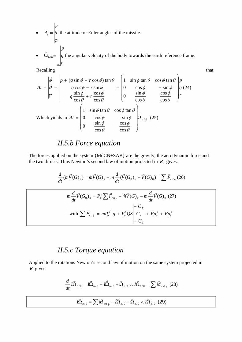
II.5.c Torque equation
Applied to the rotations Newton’s second law of motion on the same system projected in
bR gives:
bextbbbbb MIIIIdtd ∑=Ω∧Ω+Ω+Ω=Ω
rrr&rr&
r0/0/0/0/0/ (28)
0/0/0/0/ bbbbextb IIMI Ω∧Ω−Ω−=Ω ∑rrr
&r&r (29)
with br
bl
n
m
l
bext pMpMCCC
QSMrrr
++=∑
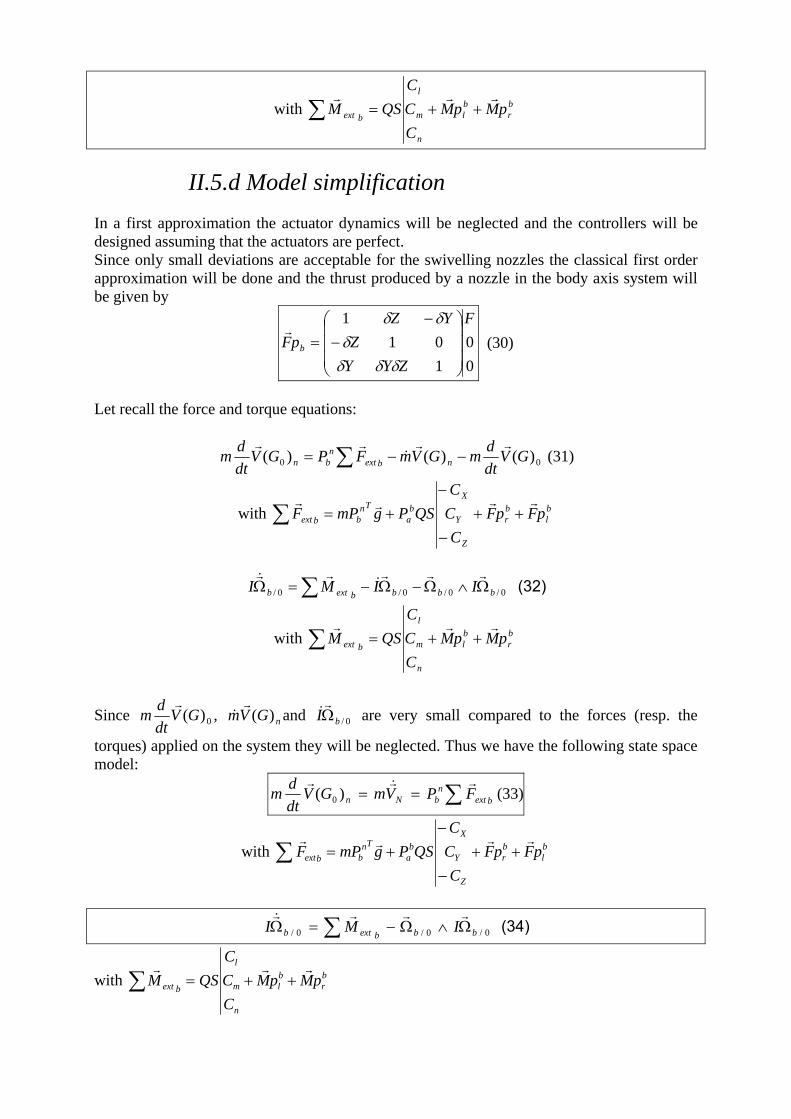
II.5.d Model simplification
In a first approximation the actuator dynamics will be neglected and the controllers will be designed assuming that the actuators are perfect. Since only small deviations are acceptable for the swivelling nozzles the classical first order approximation will be done and the thrust produced by a nozzle in the body axis system will be given by
00
101
1 F
ZYYZ
YZpF b
⎟⎟⎟
⎠
⎞
⎜⎜⎜
⎝
⎛−
−=
δδδδ
δδr
(30)
Let recall the force and torque equations:
00 )()()( GVdtdmGVmFPGV
dtdm nbext
nbn
rr&
rr−−= ∑ (31)
with bl
br
Z
Y
Xb
aTn
bbext pFpFC
CC
QSPgmPFrrrr
++−
−+=∑
0/0/0/0/ bbbbextb IIMI Ω∧Ω−Ω−=Ω ∑rrr
&r&r (32)
with br
bl
n
m
l
bext pMpMCCC
QSMrrr
++=∑
Since 0)(GVdtdmr
, nGVm )(r
& and 0/bIΩr& are very small compared to the forces (resp. the
torques) applied on the system they will be neglected. Thus we have the following state space model:
∑== bextn
bNn FPVmGVdtdm
r&rr)( 0 (33)
with bl
br
Z
Y
Xb
aTn
bbext pFpFC
CC
QSPgmPFrrrr
++−
−+=∑
0/0/0/ bbbextb IMI Ω∧Ω−=Ω ∑rrr&r (34)
with br
bl
n
m
l
bext pMpMCCC
QSMrrr
++=∑
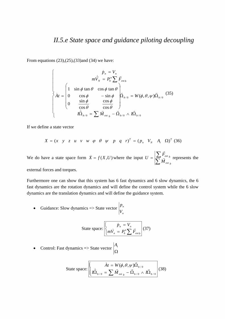
II.5.e State space and guidance piloting decoupling
From equations (23),(25),(33)and (34) we have:
⎪⎪⎪⎪
⎩
⎪⎪⎪⎪
⎨
⎧
Ω∧Ω−=Ω
Ω=Ω
⎟⎟⎟⎟⎟
⎠
⎞
⎜⎜⎜⎜⎜
⎝
⎛
−=
=
=
∑
∑
0/0/0/
0/0/ ),,(
coscos
cossin0
sincos0tancostansin1
bbbextb
bb
bextn
bN
nn
IMI
WtA
FPVmVp
rrr&r
rr&
r&r&
ψθφ
θφ
θφ
φφθφθφ
(35)
If we define a state vector
TtNn
T AVprqpwvuzyxX )()( Ω== ψθϕ (36)
We do have a state space form ),( UXfX =& where the input bext
bext
MF
U∑∑= r
r
represents the
external forces and torques.
Furthermore one can show that this system has 6 fast dynamics and 6 slow dynamics, the 6 fast dynamics are the rotation dynamics and will define the control system while the 6 slow dynamics are the translation dynamics and will define the guidance system.
• Guidance: Slow dynamics => State vector n
n
Vp
State space: ⎩⎨⎧
==
∑ bextn
bn
nn
FPVmVp
r&
& (37)
• Control: Fast dynamics => State vector Ω
tA
State space: ⎪⎩
⎪⎨⎧
Ω∧Ω−=Ω
Ω=
∑ 0/0/0/
0/),,(
bbbextb
b
IMIWtA
rrr&r
r& ψθφ
(38)
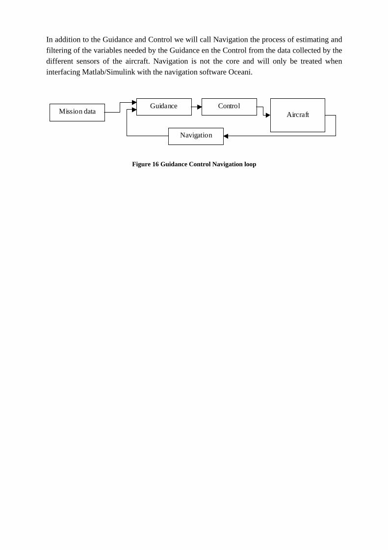
In addition to the Guidance and Control we will call Navigation the process of estimating and filtering of the variables needed by the Guidance en the Control from the data collected by the different sensors of the aircraft. Navigation is not the core and will only be treated when interfacing Matlab/Simulink with the navigation software Oceani.
Mission data
Guidance
Control
Navigation
Aircraft
Figure 16 Guidance Control Navigation loop
III. Launch phase
III.1 The launch phase. The main challenge during the launch phase is the lack of control inputs. The only thing that can be commanded during this phase is the orientation of the nozzles. There is no control on the magnitude of the thrust; the wings and fins are not available yet so the missile can’t be controlled using rudder deflections. It is decided to use the deviation of the thrust to control the attitude of the missile. During a first phase ( s5.1≈ ) the missile will accelerate in a vertical position and then turns over to a horizontal trajectory. During the swing the angle of attack (AoA) of the missile may grow a lot and this can cause stall phenomenon or make the ignition of the turbojet impossible. This leads us to the other requirements of the phase: the angle of attack should keep reasonable values and be as small as possible when the turbojet is ignited at the end of the launch phase, the speed of the missile should be high enough to ignite the turbojet and finally to avoid detection by potential enemies the missile should stay below 500m.
III.2 First controller design In this part a first controller for the launch phase is designed. To accomplish this task it was decided to use a Lyapunov theory based technique called backstepping. Indeed the equations that describe the behaviour of the missile are highly non-linear so it is natural to use a nonlinear controller. Usually the industrials uses gain scheduling to deal with this issue, so gain-scheduled controller will not be investigated here. A Lyapunov theory based technique called back-stepping gave already promising results in previous studies of the DGA focusing on UAV guidance and control [11] and it was decided to investigate further whether or not this technique could give good results applied on the launch phase of the MdCN. Feedback linearization, Sliding modes based controllers or optimal controller using Pontryagin’s Maximum Principle for example were other options but previous studies held at the DGA showed that feedback linearizing controller had poor behaviour in terms of robustness and external disturbances rejection. Furthermore sliding modes controller would have needed very fast switch of the control signal around a sliding surface which might be hard to achieve with the future nozzle actuators of the booster. This actuator has not been studied that much for now but the technical specification describes a low pass filter behaviour (see II.4). Concerning optimal controllers, it has to be taken in account that the system obtained are already quite complicated and has no simple explicit solution and the computational complexity required to solve the optimal control problem numerically might be to big to be implemented. One challenge of the Back-stepping technique is that it needs a system under strict-feedback form to be applied easily. In first part the back-stepping technique will be presented more in detail, then the so called quaternions are introduced and the procedure used to rewrite the state space equation will be discussed finally the backstepping design and the first results of the obtained controller are detailed.
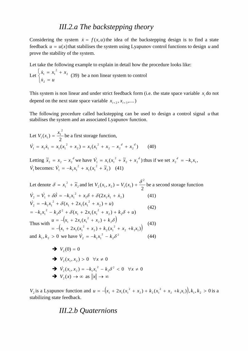
III.2.a The backstepping theory Considering the system ),( uxfx =& the idea of the backstepping design is to find a state feedback )(xuu = that stabilises the system using Lyapunov control functions to design u and prove the stability of the system. Let take the following example to explain in detail how the procedure looks like:
Let ⎩⎨⎧
=+=
uxxxx
2
22
11
&
& (39) be a non linear system to control
This system is non linear and under strict feedback form (i.e. the state space variable ix do not depend on the next state space variable ,...., 32 ++ ii xx ) The following procedure called backstepping can be used to design a control signal u that stabilises the system and an associated Lyapunov function.
Let 2
)(2
111
xxV = be a first storage function,
)()( 2222
1122
11111dd xxxxxxxxxxV +−+=+== && (40)
Letting dxxx 222
~ −= we have )~( 222
111dxxxxV ++=& thus if we set 112 xkx d −= ,
1V& becomes: )~( 22
112
111 xxxxkV ++−=& (41)
Let denote 22
1~xx +=δ and let
2)(),(
2
11212δ
+= xVxxV be a second storage function
)2( 21112
1112 xxxxxkVV &&&&& +++−=+= δδδδ (41)
))(2(
))(2(
222
1112
22
11
22
1112
112
ukxxxxkxk
uxxxxxkV
+++++−−=
++++−=
δδδ
δ& (42)
Thus with ( )
( ))()(2
)(2
1122
1222
111
222
111
xkxxkxxxx
kxxxxu
+++++−=
+++−= δ (43)
and 0, 21 >kk we have 22
2112 δkxkV −−=& (44)
0)0(2 =V
00),( 212 ≠∀> xxxV
00),( 22
211212 ≠∀<−−= xkxkxxV δ&
∞→)(2 xV as ∞→x
2V is a Lyapunov function and ( ))()(2 1122
1222
111 xkxxkxxxxu +++++−= , 0, 21 >kk is a stabilizing state feedback.
III.2.b Quaternions
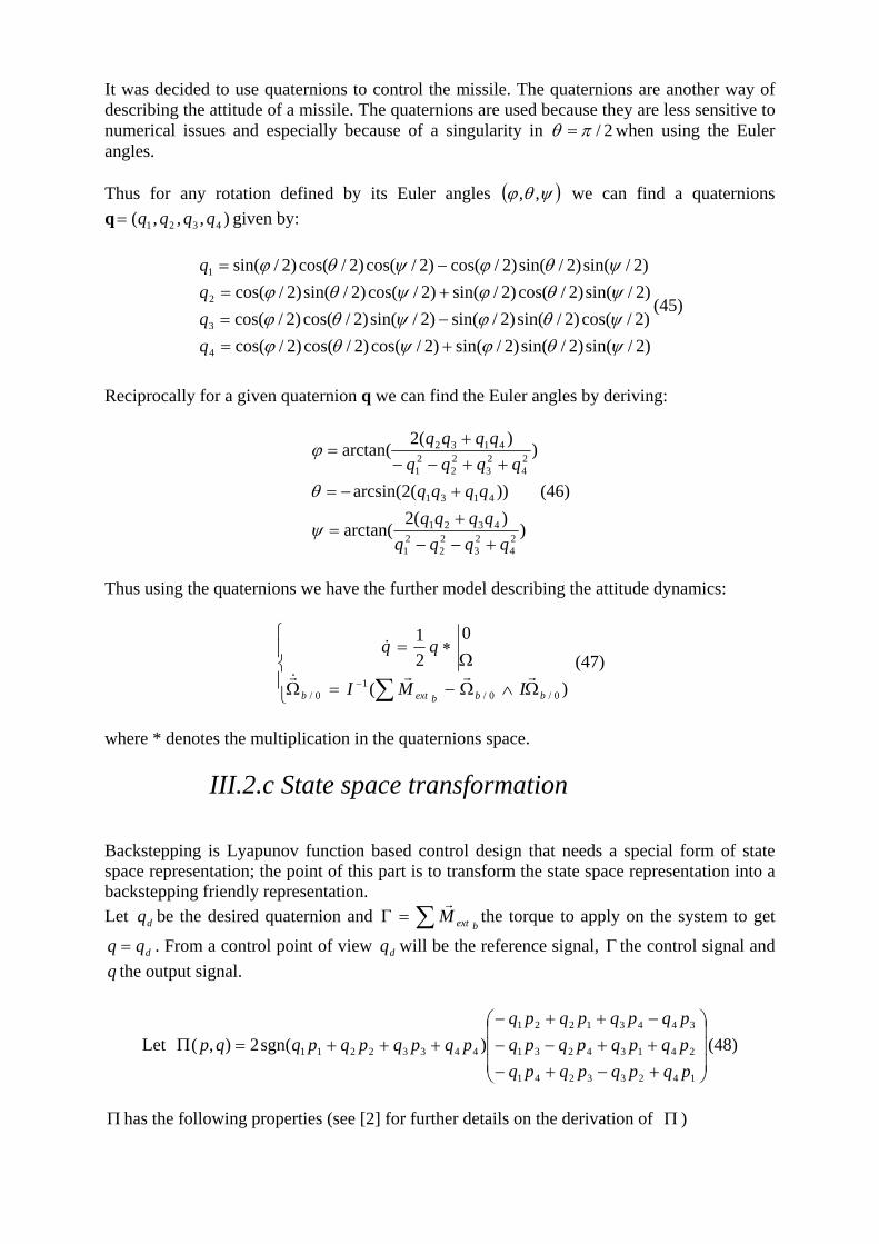
It was decided to use quaternions to control the missile. The quaternions are another way of describing the attitude of a missile. The quaternions are used because they are less sensitive to numerical issues and especially because of a singularity in 2/πθ = when using the Euler angles. Thus for any rotation defined by its Euler angles ( )ψθϕ ,, we can find a quaternions q ),,,( 4321 qqqq= given by:
)2/sin()2/sin()2/sin()2/cos()2/cos()2/cos()2/cos()2/sin()2/sin()2/sin()2/cos()2/cos()2/sin()2/cos()2/sin()2/cos()2/sin()2/cos()2/sin()2/sin()2/cos()2/cos()2/cos()2/sin(
4
3
2
1
ψθϕψθϕψθϕψθϕψθϕψθϕψθϕψθϕ
+=−=+=−=
qqqq
(45)
Reciprocally for a given quaternion q we can find the Euler angles by deriving:
))(2
arctan(
))(2arcsin(
))(2
arctan(
24
23
22
21
4321
4131
24
23
22
21
4132
qqqqqqqq
qqqqqqqq
qqqq
+−−+
=
+−=++−−
+=
ψ
θ
ϕ
(46)
Thus using the quaternions we have the further model describing the attitude dynamics:
⎪⎩
⎪⎨
⎧
Ω∧Ω−=Ω
Ω∗=
∑− )(
021
0/0/1
0/ bbbextb IMI
qqrrr&r
& (47)
where * denotes the multiplication in the quaternions space.
III.2.c State space transformation Backstepping is Lyapunov function based control design that needs a special form of state space representation; the point of this part is to transform the state space representation into a backstepping friendly representation. Let dq be the desired quaternion and
bextM∑=Γr
the torque to apply on the system to get
dqq = . From a control point of view dq will be the reference signal, Γ the control signal and q the output signal.
Let ⎟⎟⎟
⎠
⎞
⎜⎜⎜
⎝
⎛
+−+−++−−−++−
+++=Π
14233241
24134231
34431221
44332211 )sgn(2),(pqpqpqpqpqpqpqpqpqpqpqpq
pqpqpqpqqp (48)
Π has the following properties (see [2] for further details on the derivation of Π )
⎪⎩
⎪⎨⎧
Ω=Π
=⇔=Π
),(0),(
d
dd
qqqqqq
&(49)
so letting Π be our new state space variable, the system becomes:
⎥⎦
⎤⎢⎣
⎡
Ω∧Ω−ΓΩ
=⎥⎦
⎤⎢⎣
⎡
Ω
Π− )(
),(
0/0/1
0/
0/ bb
b
b
d
IIqq
rr
r
&r&
(50)
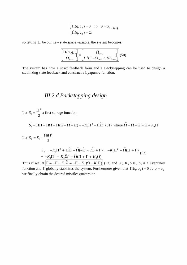
The system has now a strict feedback form and a Backstepping can be used to design a stabilizing state feedback and construct a Lyapunov function.
III.2.d Backstepping design
Let 2
2
1Π
=S a first storage function.
ΩΠ+Π−=Ω+Ω−ΩΠ=ΠΩ=ΠΠ= ~)( 2
11 KS && (51) where Π+Ω=Ω−Ω=Ω 1~ K
Let 2
~~12
tISS ΩΩ+=
)~(~~)(~)~~(~~
22
22
1
21
212
Ω+Γ+ΠΩ+Ω−Π−=
Γ+ΠΩ+Π−=Γ+Ω∧Ω−Ω+ΩΠ+Π−=
KKK
KIKS& (52)
Thus if we let )(~122 Π−Ω−Π−=Ω−Π−=Γ KKK (53) and 0, 21 >KK , 2S is a Lyapunov
function and Γ globally stabilizes the system. Furthermore given that dd qqqq =⇔=Π 0),( we finally obtain the desired missiles quaternion.
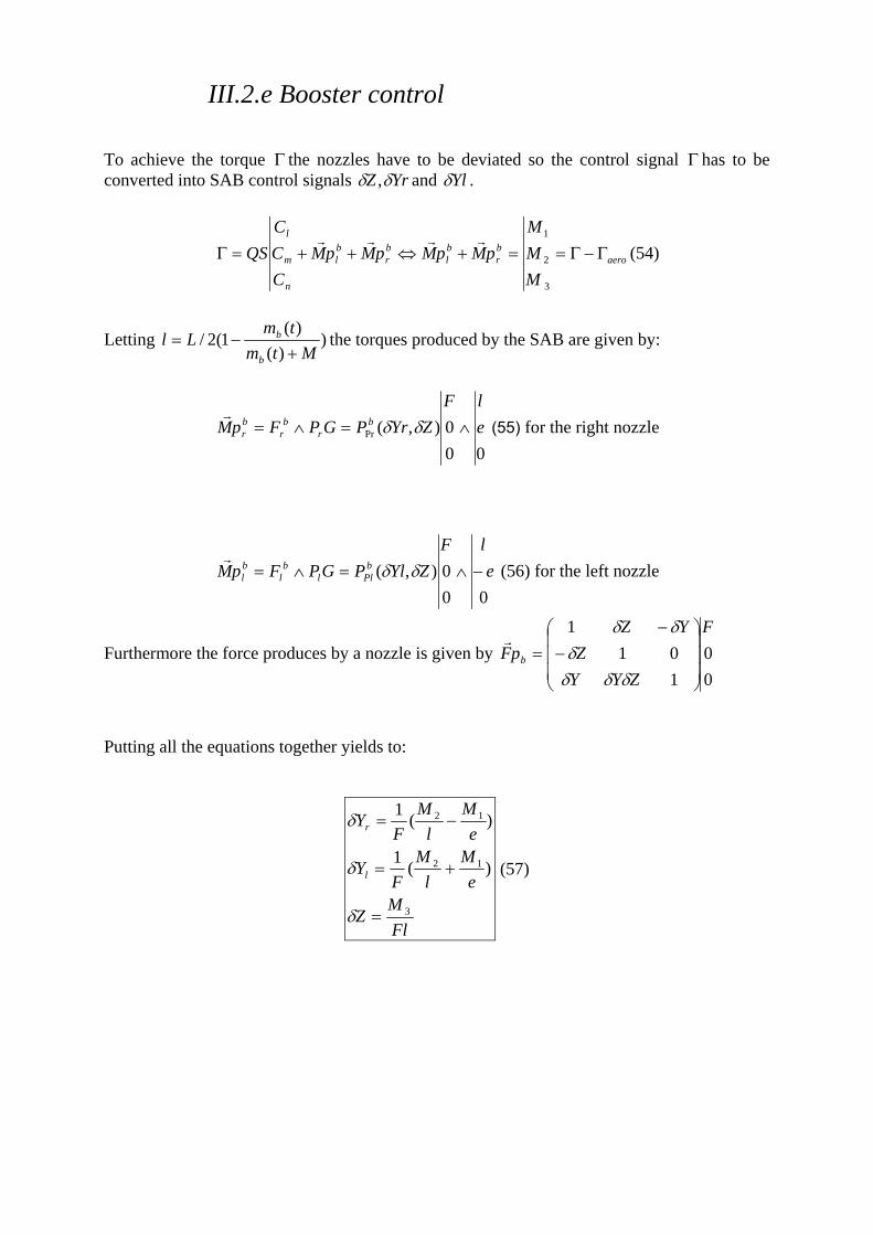
III.2.e Booster control To achieve the torque Γ the nozzles have to be deviated so the control signal Γ has to be converted into SAB control signals YrZ δδ , and Ylδ .
aerobr
bl
br
bl
n
m
l
MMM
pMpMpMpMCCC
QS Γ−Γ==+⇔++=Γ
3
2
1rrrr(54)
Letting ))(
)(1(2/
Mtmtm
Llb
b
+−= the torques produced by the SAB are given by:
000),(Pr e
lFZYrPGPFpM b
rb
rbr ∧=∧= δδ
r (55) for the right nozzle
000),( e
lFZYlPGPFpM b
Pllb
lbl −∧=∧= δδ
r (56) for the left nozzle
Furthermore the force produces by a nozzle is given by 00
101
1 F
ZYYZ
YZpF b
⎟⎟⎟
⎠
⎞
⎜⎜⎜
⎝
⎛−
−=
δδδδ
δδr
Putting all the equations together yields to:
FlM
Z
eM
lM
FY
eM
lM
FY
l
r
3
12
12
)(1
)(1
=
+=
−=
δ
δ
δ
(57)
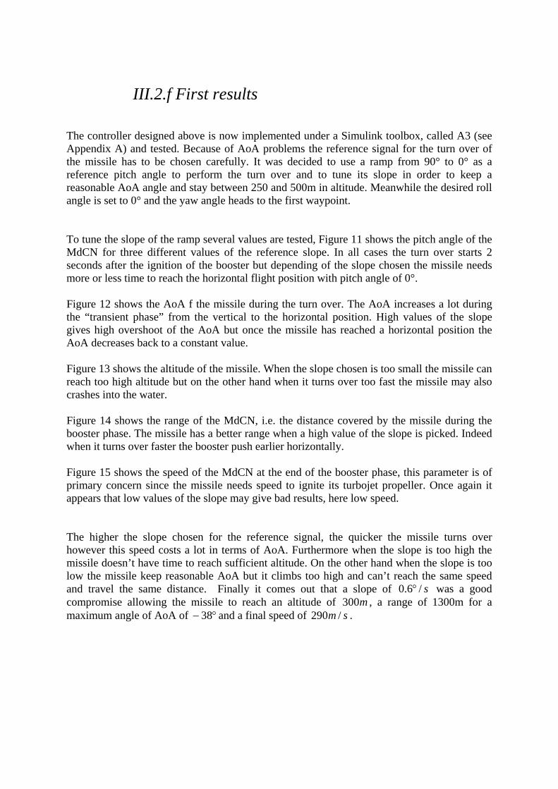
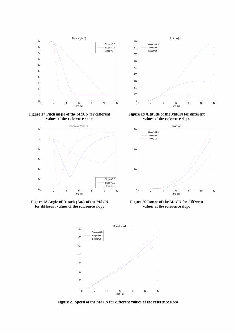
III.2.f First results The controller designed above is now implemented under a Simulink toolbox, called A3 (see Appendix A) and tested. Because of AoA problems the reference signal for the turn over of the missile has to be chosen carefully. It was decided to use a ramp from 90° to 0° as a reference pitch angle to perform the turn over and to tune its slope in order to keep a reasonable AoA angle and stay between 250 and 500m in altitude. Meanwhile the desired roll angle is set to 0° and the yaw angle heads to the first waypoint. To tune the slope of the ramp several values are tested, Figure 11 shows the pitch angle of the MdCN for three different values of the reference slope. In all cases the turn over starts 2 seconds after the ignition of the booster but depending of the slope chosen the missile needs more or less time to reach the horizontal flight position with pitch angle of 0°. Figure 12 shows the AoA f the missile during the turn over. The AoA increases a lot during the “transient phase” from the vertical to the horizontal position. High values of the slope gives high overshoot of the AoA but once the missile has reached a horizontal position the AoA decreases back to a constant value. Figure 13 shows the altitude of the missile. When the slope chosen is too small the missile can reach too high altitude but on the other hand when it turns over too fast the missile may also crashes into the water. Figure 14 shows the range of the MdCN, i.e. the distance covered by the missile during the booster phase. The missile has a better range when a high value of the slope is picked. Indeed when it turns over faster the booster push earlier horizontally. Figure 15 shows the speed of the MdCN at the end of the booster phase, this parameter is of primary concern since the missile needs speed to ignite its turbojet propeller. Once again it appears that low values of the slope may give bad results, here low speed. The higher the slope chosen for the reference signal, the quicker the missile turns over however this speed costs a lot in terms of AoA. Furthermore when the slope is too high the missile doesn’t have time to reach sufficient altitude. On the other hand when the slope is too low the missile keep reasonable AoA but it climbs too high and can’t reach the same speed and travel the same distance. Finally it comes out that a slope of s/6.0 ° was a good compromise allowing the missile to reach an altitude of m300 , a range of 1300m for a maximum angle of AoA of °− 38 and a final speed of sm /290 .
0 2 4 6 8 10 12-10
0
10
20
30
40
50
60
70
80
90Pitch angle [°]
time [s]
Slope=0.6Slope=0.2Slope=2
Figure 17 Pitch angle of the MdCN for different
values of the reference slope
0 2 4 6 8 10 12-50
-40
-30
-20
-10
0
10incidence angle [°]
time [s]
Slope=0.6Slope=0.2Slope=2
Figure 18 Angle of Attack (AoA of the MdCN
for different values of the reference slope
0 2 4 6 8 10 120
100
200
300
400
500
600
700
800
900Altitude [m]
time [s]
Slope=0.6Slope=0.2Slope=2
Figure 19 Altitude of the MdCN for different
values of the reference slope
0 2 4 6 8 10 120
500
1000
1500Range [m]
time [s]
Slope=0.6Slope=0.2Slope=2
Figure 20 Range of the MdCN for different
values of the reference slope
0 2 4 6 8 10 120
50
100
150
200
250
300
350Speed [m/s]
time [s]
Slope=0.6Slope=0.2Slope=2
Figure 21 Speed of the MdCN for different values of the reference slope
III.3 Controller improvement The results of the previous controller were good but still it doesn’t guarantee that by the end of the booster phase the missile is in optimal conditions to ignite the turbojet, we have for example no control on the final values of the AoA of the missile at the end of the booster phase, so it was decided to use a special sequence in the reference signal of the previous controller. This choice was motivated by the simplicity of its implementation. This part describes the procedure used to improve the previous controller based on the new control sequence and a statistic analysis of the parameters of this sequence by Monte Carlo simulations.
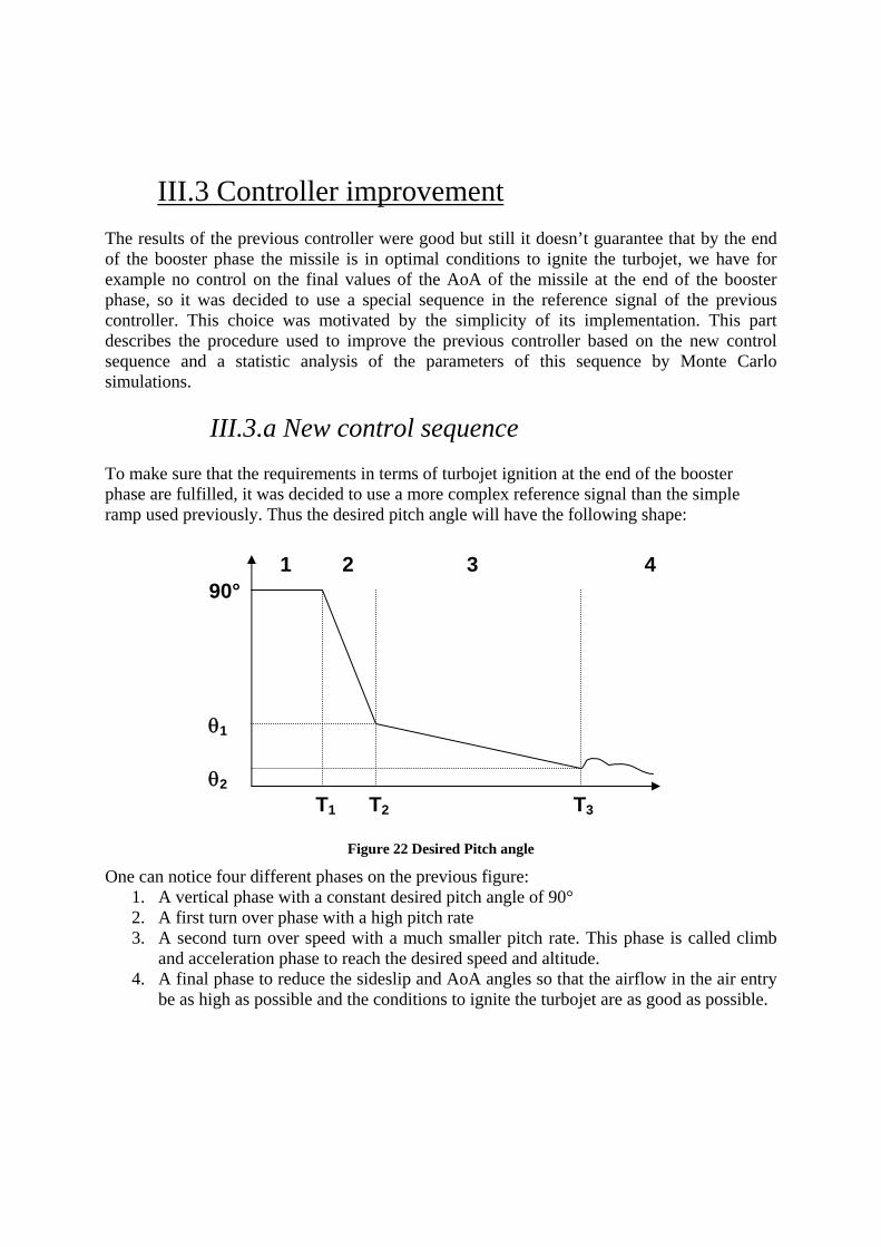
III.3.a New control sequence To make sure that the requirements in terms of turbojet ignition at the end of the booster phase are fulfilled, it was decided to use a more complex reference signal than the simple ramp used previously. Thus the desired pitch angle will have the following shape:
Figure 22 Desired Pitch angle
One can notice four different phases on the previous figure: 1. A vertical phase with a constant desired pitch angle of 90° 2. A first turn over phase with a high pitch rate 3. A second turn over speed with a much smaller pitch rate. This phase is called climb
and acceleration phase to reach the desired speed and altitude. 4. A final phase to reduce the sideslip and AoA angles so that the airflow in the air entry
be as high as possible and the conditions to ignite the turbojet are as good as possible.
3 2 1 4
T1 T2 T3
θ1
90°
θ2
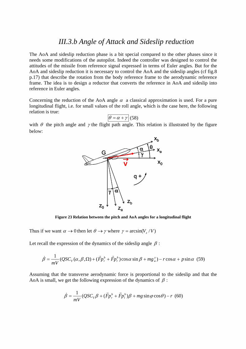
III.3.b Angle of Attack and Sideslip reduction The AoA and sideslip reduction phase is a bit special compared to the other phases since it needs some modifications of the autopilot. Indeed the controller was designed to control the attitudes of the missile from reference signal expressed in terms of Euler angles. But for the AoA and sideslip reduction it is necessary to control the AoA and the sideslip angles (cf fig.8 p.17) that describe the rotation from the body reference frame to the aerodynamic reference frame. The idea is to design a reductor that converts the reference in AoA and sideslip into reference in Euler angles. Concerning the reduction of the AoA angle α a classical approximation is used. For a pure longitudinal flight, i.e. for small values of the roll angle, which is the case here, the following relation is true:
γαθ += (58) with θ the pitch angle and γ the flight path angle. This relation is illustrated by the figure below:
γα θ
xb
G
zb
x0
z0
xa
za
→V
γ α
q +
γα θ
xb
G
zb
x0
z0
xa
za
→V→→V
γ α
q +
Figure 23 Relation between the pitch and AoA angles for a longitudinal flight
Thus if we want 0→α then let γθ → where )/arcsin( VVz=γ Let recall the expression of the dynamics of the sideslip angle β :
ααβαβαβ sincos)sincos)(),,((1 prmgpFpFQSCmV
yw
bl
brY +−+++Ω=
rr& (59)
Assuming that the transverse aerodynamic force is proportional to the sideslip and that the AoA is small, we get the following expression of the dynamics of β :
rmgpFpFQSCmV
bl
brY −+++= )cossin)((1 θϕβββ
rr& (60)
Furthermore for small values of the roll we have r≈ψ& thus the dynamics of β become:
ψθβββ &rr
& −+++= )cos)((1 mgpFpFQSCmV
bl
brY (61)
Letting ψθ&−=
Vgu cos be a new control variable and )(1 b
lbrY pFpFQSC
mVa
rr++= we have
the following system ua += ββ& which will be controlled using the state feedback βτ )( +−= au with τ the desired time constant of the sideslip angle.
Finally the commanded yaw angle will be WPdtV
ga ψθβτψ +⎟⎠⎞
⎜⎝⎛ ++= ∫
cos)( (62) where
WPψ is the yaw angle to the next waypoint.
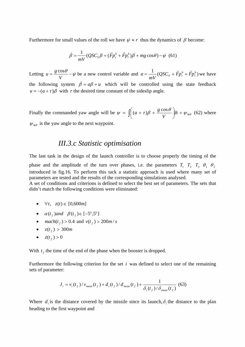
III.3.c Statistic optimisation The last task in the design of the launch controller is to choose properly the timing of the
phase and the amplitude of the turn over phases, i.e. the parameters 21321 θθTTT introduced in fig.16. To perform this tack a statistic approach is used where many set of parameters are tested and the results of the corresponding simulations analysed. A set of conditions and criterions is defined to select the best set of parameters. The sets that didn’t match the following conditions were eliminated:
• ]600,0[)(, mtzt ∈∀
• ]5,5[)()( °°−∈ff tandt βα • 4.0)( >ftmach and smtv f /200)( > • mtz f 300)( > • 0)( >ftz&
With ft the time of the end of the phase when the booster is dropped. Furthermore the following criterion for the set i was defined to select one of the remaining sets of parameter:
)(/)(1)(/)()(/)(
fmeanfifmeanfifmeanfii tt
tdtdtvtvJδδ
++= (63)
Where id is the distance covered by the missile since its launch, iδ the distance to the plan heading to the first waypoint and
∑∑∈∈
==],1[],1[
1,1ni
imeanni
imean dn
dvn
v and ∑∈
=],1[
1ni
imean nδδ are the mean value of respectively
the speed, distance covered and distance to the desired plan on the sets matching the conditions introduced above.
Figure 24 Distances to the optimal trajectory
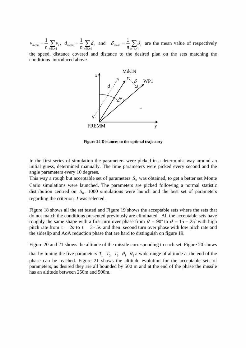
In the first series of simulation the parameters were picked in a determinist way around an initial guess, determined manually. The time parameters were picked every second and the angle parameters every 10 degrees. This way a rough but acceptable set of parameters 0S was obtained, to get a better set Monte Carlo simulations were launched. The parameters are picked following a normal statistic distribution centred on 0S . 1000 simulations were launch and the best set of parameters regarding the criterion J was selected. Figure 18 shows all the set tested and Figure 19 shows the acceptable sets where the sets that do not match the conditions presented previously are eliminated. All the acceptable sets have roughly the same shape with a first turn over phase from °= 90θ to °−= 2515θ with high pitch rate from 2st = to 5s- 3t = and then second turn over phase with low pitch rate and the sideslip and AoA reduction phase that are hard to distinguish on figure 19. Figure 20 and 21 shows the altitude of the missile corresponding to each set. Figure 20 shows
that by tuning the five parameters 21321 θθTTT a wide range of altitude at the end of the phase can be reached. Figure 21 shows the altitude evolution for the acceptable sets of parameters, as desired they are all bounded by 500 m and at the end of the phase the missile has an altitude between 250m and 500m.
δ
MdCN
cψ
WP1 x
y FREMM
δd
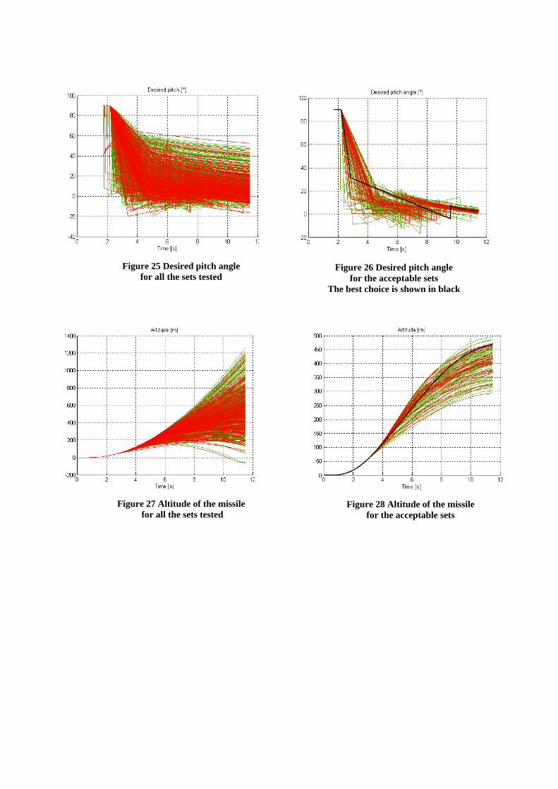
Figure 25 Desired pitch angle
for all the sets tested
Figure 26 Desired pitch angle
for the acceptable sets The best choice is shown in black
Figure 27 Altitude of the missile
for all the sets tested
Figure 28 Altitude of the missile
for the acceptable sets
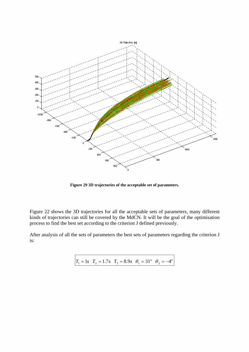
Figure 29 3D trajectories of the acceptable set of parameters.
Figure 22 shows the 3D trajectories for all the acceptable sets of parameters, many different kinds of trajectories can still be covered by the MdCN. It will be the goal of the optimisation process to find the best set according to the criterion J defined previously. After analysis of all the sets of parameters the best sets of parameters regarding the criterion J is:
°−=°==== 4319.87.11 21321 θθsTsTsT
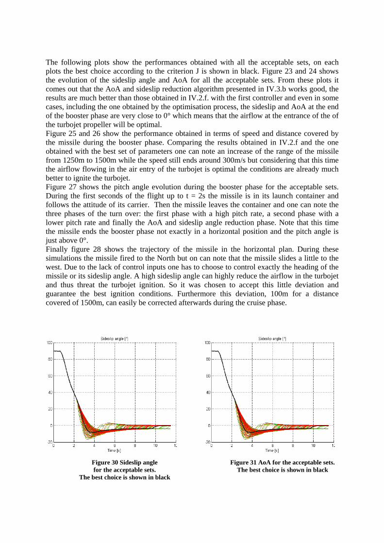
The following plots show the performances obtained with all the acceptable sets, on each plots the best choice according to the criterion J is shown in black. Figure 23 and 24 shows the evolution of the sideslip angle and AoA for all the acceptable sets. From these plots it comes out that the AoA and sideslip reduction algorithm presented in IV.3.b works good, the results are much better than those obtained in IV.2.f. with the first controller and even in some cases, including the one obtained by the optimisation process, the sideslip and AoA at the end of the booster phase are very close to 0° which means that the airflow at the entrance of the of the turbojet propeller will be optimal. Figure 25 and 26 show the performance obtained in terms of speed and distance covered by the missile during the booster phase. Comparing the results obtained in IV.2.f and the one obtained with the best set of parameters one can note an increase of the range of the missile from 1250m to 1500m while the speed still ends around 300m/s but considering that this time the airflow flowing in the air entry of the turbojet is optimal the conditions are already much better to ignite the turbojet. Figure 27 shows the pitch angle evolution during the booster phase for the acceptable sets. During the first seconds of the flight up to t = 2s the missile is in its launch container and follows the attitude of its carrier. Then the missile leaves the container and one can note the three phases of the turn over: the first phase with a high pitch rate, a second phase with a lower pitch rate and finally the AoA and sideslip angle reduction phase. Note that this time the missile ends the booster phase not exactly in a horizontal position and the pitch angle is just above 0°. Finally figure 28 shows the trajectory of the missile in the horizontal plan. During these simulations the missile fired to the North but on can note that the missile slides a little to the west. Due to the lack of control inputs one has to choose to control exactly the heading of the missile or its sideslip angle. A high sideslip angle can highly reduce the airflow in the turbojet and thus threat the turbojet ignition. So it was chosen to accept this little deviation and guarantee the best ignition conditions. Furthermore this deviation, 100m for a distance covered of 1500m, can easily be corrected afterwards during the cruise phase.
Figure 30 Sideslip angle for the acceptable sets.
The best choice is shown in black
Figure 31 AoA for the acceptable sets.
The best choice is shown in black
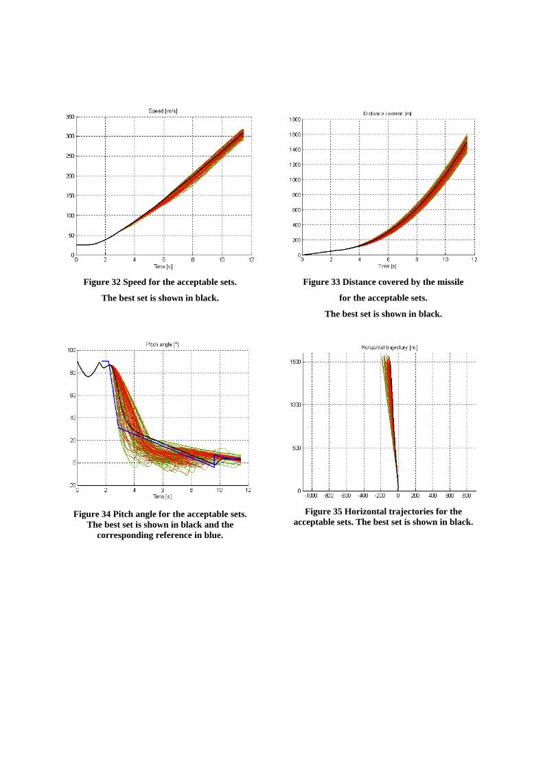
Figure 32 Speed for the acceptable sets.
The best set is shown in black.
Figure 33 Distance covered by the missile
for the acceptable sets.
The best set is shown in black.
Figure 34 Pitch angle for the acceptable sets.
The best set is shown in black and the corresponding reference in blue.
Figure 35 Horizontal trajectories for the
acceptable sets. The best set is shown in black.
III.4 Performance analysis The performances of the selected set of parameters are now tested under several external conditions to evaluate the performance of the control law obtained and determined whether or not the missile can be fired under this conditions.
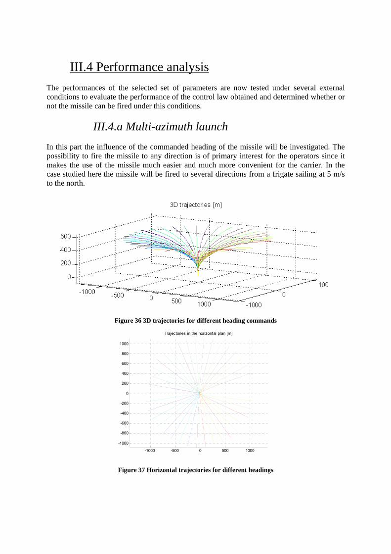
III.4.a Multi-azimuth launch In this part the influence of the commanded heading of the missile will be investigated. The possibility to fire the missile to any direction is of primary interest for the operators since it makes the use of the missile much easier and much more convenient for the carrier. In the case studied here the missile will be fired to several directions from a frigate sailing at 5 m/s to the north.
Figure 36 3D trajectories for different heading commands
-1000 -500 0 500 1000
-1000
-800
-600
-400
-200
0
200
400
600
800
1000
Trajectories in the horizontal plan [m]
Figure 37 Horizontal trajectories for different headings

0 2 4 6 8 10 120
100
200
300
400
500
600Altitude [m]
Time [s] Figure 38Altitude for different headings
0 2 4 6 8 10 120
50
100
150
200
250
300
Time [s]
Speed [m/s]
Figure 39 Speed for different headings
0 2 4 6 8 10 12-100
-80
-60
-40
-20
0
20
40
60
80
100
Time [s]
AoA [°]
Figure 40 Angle of Attack for different headings
0 2 4 6 8 10 12-40
-20
0
20
40
60
80
100
Time [s]
Sideslip angles [°]
Figure 41 Sideslip angle for different headings
Figure 29 and 30 show the trajectories of the missile in 3D and in the horizontal plan while Figure 31 shows the altitude of the missile. From these three plots it comes out that the missile follows in every case the same kind of trajectory, except for the heading of course, that seems to match the requirements of the launch phase. Now it has to be checked that the conditions to ignite the turbojet are good. This is done by studying figure 32, 33 and 34 showing the speed, AoA and sideslip angle of the missile during the booster phase. In all cases the missile reaches good conditions to ignite the turbojet. With the controller obtained the altitude and speed are almost not sensitive to the heading commanded. It is also interesting to note that the AoA and sideslip angles reductors designed in III.3.b work well for various commanded headings.
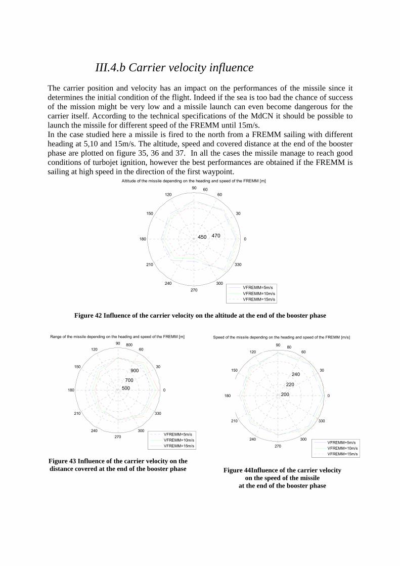
III.4.b Carrier velocity influence The carrier position and velocity has an impact on the performances of the missile since it determines the initial condition of the flight. Indeed if the sea is too bad the chance of success of the mission might be very low and a missile launch can even become dangerous for the carrier itself. According to the technical specifications of the MdCN it should be possible to launch the missile for different speed of the FREMM until 15m/s. In the case studied here a missile is fired to the north from a FREMM sailing with different heading at 5,10 and 15m/s. The altitude, speed and covered distance at the end of the booster phase are plotted on figure 35, 36 and 37. In all the cases the missile manage to reach good conditions of turbojet ignition, however the best performances are obtained if the FREMM is sailing at high speed in the direction of the first waypoint.
450 470
60
30
210
60
240
90
270
120
300
150
330
180 0
Altitude of the missile depending on the heading and speed of the FREMM [m]
VFREMM=5m/sVFREMM=10m/sVFREMM=15m/s
Figure 42 Influence of the carrier velocity on the altitude at the end of the booster phase
500 700
900
800
30
210
60
240
90
270
120
300
150
330
180 0
Range of the missile depending on the heading and speed of the FREMM [m]
VFREMM=5m/sVFREMM=10m/sVFREMM=15m/s
Figure 43 Influence of the carrier velocity on the distance covered at the end of the booster phase
200
220
240
80
30
210
60
240
90
270
120
300
150
330
180 0
Speed of the missile depending on the heading and speed of the FREMM [m/s]
VFREMM=5m/sVFREMM=10m/sVFREMM=15m/s
Figure 44Influence of the carrier velocity
on the speed of the missile at the end of the booster phase
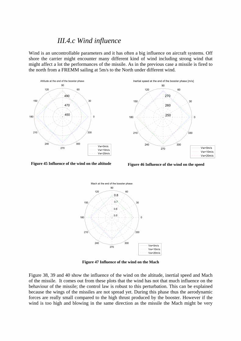
III.4.c Wind influence Wind is an uncontrollable parameters and it has often a big influence on aircraft systems. Off shore the carrier might encounter many different kind of wind including strong wind that might affect a lot the performances of the missile. As in the previous case a missile is fired to the north from a FREMM sailing at 5m/s to the North under different wind.
450
470
49030
210
60
240
90
270
120
300
150
330
180 0
Altitude at the end of the booster phase
Vw=0m/sVw=10m/sVw=20m/s
Figure 45 Influence of the wind on the altitude
250
260
27030
210
60
240
90
270
120
300
150
330
180 0
Inertial speed at the end of the booster phase [m/s]
Vw=0m/sVw=10m/sVw=20m/s
Figure 46 Influence of the wind on the speed
0.5
0.6
0.7
0.8
30
210
60
240
90
270
120
300
150
330
180 0
Mach at the end of the booster phase
Vw=0m/sVw=10m/sVw=20m/s
Figure 47 Influence of the wind on the Mach
Figure 38, 39 and 40 show the influence of the wind on the altitude, inertial speed and Mach of the missile. It comes out from these plots that the wind has not that much influence on the behaviour of the missile; the control law is robust to this perturbation. This can be explained because the wings of the missiles are not spread yet. During this phase thus the aerodynamic forces are really small compared to the high thrust produced by the booster. However if the wind is too high and blowing in the same direction as the missile the Mach might be very
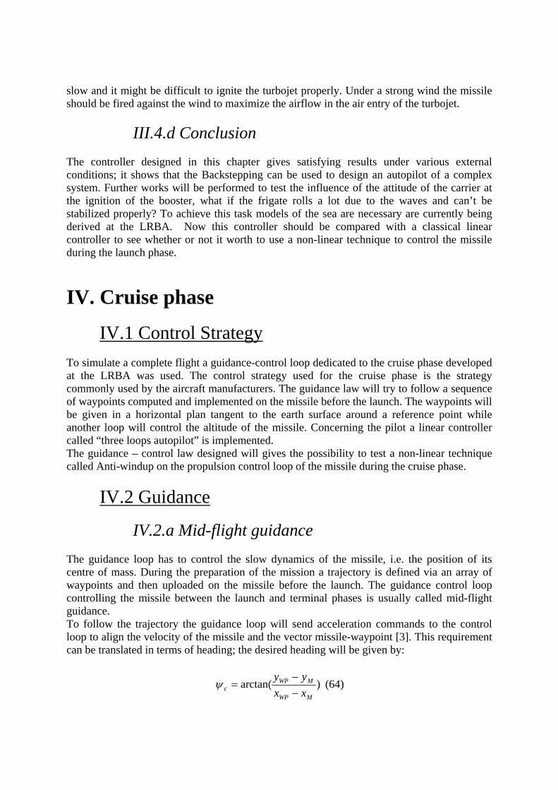
slow and it might be difficult to ignite the turbojet properly. Under a strong wind the missile should be fired against the wind to maximize the airflow in the air entry of the turbojet.
III.4.d Conclusion The controller designed in this chapter gives satisfying results under various external conditions; it shows that the Backstepping can be used to design an autopilot of a complex system. Further works will be performed to test the influence of the attitude of the carrier at the ignition of the booster, what if the frigate rolls a lot due to the waves and can’t be stabilized properly? To achieve this task models of the sea are necessary are currently being derived at the LRBA. Now this controller should be compared with a classical linear controller to see whether or not it worth to use a non-linear technique to control the missile during the launch phase.
IV. Cruise phase
IV.1 Control Strategy To simulate a complete flight a guidance-control loop dedicated to the cruise phase developed at the LRBA was used. The control strategy used for the cruise phase is the strategy commonly used by the aircraft manufacturers. The guidance law will try to follow a sequence of waypoints computed and implemented on the missile before the launch. The waypoints will be given in a horizontal plan tangent to the earth surface around a reference point while another loop will control the altitude of the missile. Concerning the pilot a linear controller called “three loops autopilot” is implemented. The guidance – control law designed will gives the possibility to test a non-linear technique called Anti-windup on the propulsion control loop of the missile during the cruise phase.
IV.2 Guidance
IV.2.a Mid-flight guidance The guidance loop has to control the slow dynamics of the missile, i.e. the position of its centre of mass. During the preparation of the mission a trajectory is defined via an array of waypoints and then uploaded on the missile before the launch. The guidance control loop controlling the missile between the launch and terminal phases is usually called mid-flight guidance. To follow the trajectory the guidance loop will send acceleration commands to the control loop to align the velocity of the missile and the vector missile-waypoint [3]. This requirement can be translated in terms of heading; the desired heading will be given by:
)arctan(MWP
MWPc xx
yy−−
=ψ (64)
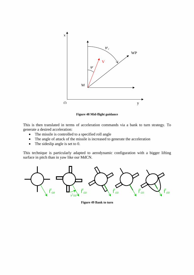
Figure 48 Mid-flight guidance
This is then translated in terms of acceleration commands via a bank to turn strategy. To generate a desired acceleration:
• The missile is controlled to a specified roll angle • The angle of attack of the missile is increased to generate the acceleration • The sideslip angle is set to 0.
This technique is particularly adapted to aerodynamic configuration with a bigger lifting surface in pitch than in yaw like our MdCN.
Figure 49 Bank to turn
M
cψ WP
x
y O
ψV
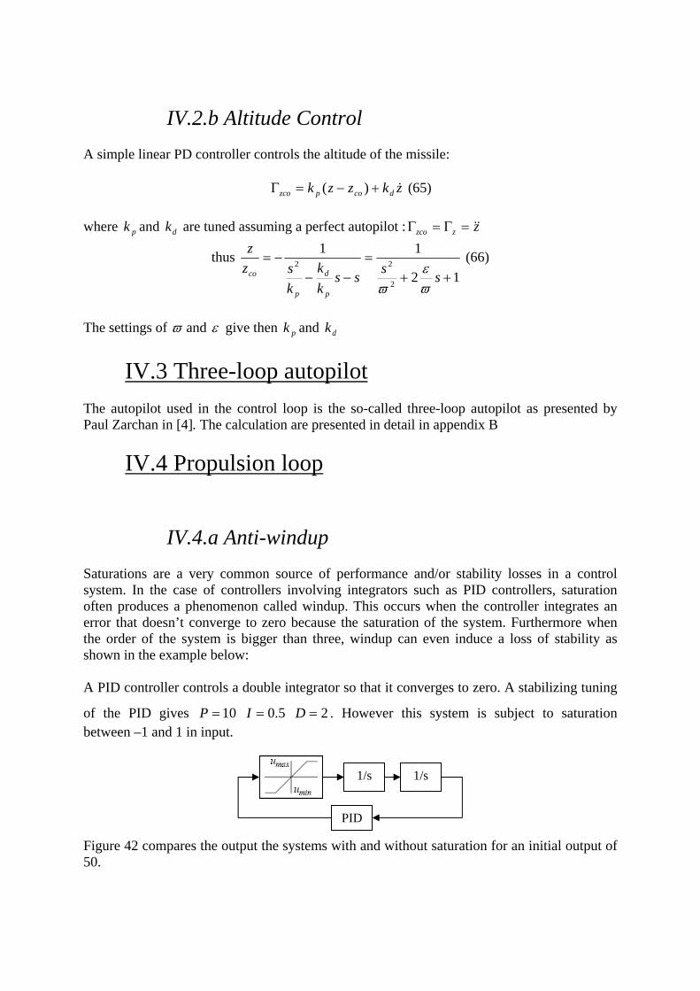
IV.2.b Altitude Control A simple linear PD controller controls the altitude of the missile:
zkzzk dcopzco &+−=Γ )( (65)
where pk and dk are tuned assuming a perfect autopilot : zzzco &&=Γ=Γ
thus 12
11
2
22
++=
−−−=
sssskk
ksz
z
p
d
p
co
ϖε
ϖ
(66)
The settings of ϖ and ε give then pk and dk
IV.3 Three-loop autopilot The autopilot used in the control loop is the so-called three-loop autopilot as presented by Paul Zarchan in [4]. The calculation are presented in detail in appendix B
IV.4 Propulsion loop
IV.4.a Anti-windup Saturations are a very common source of performance and/or stability losses in a control system. In the case of controllers involving integrators such as PID controllers, saturation often produces a phenomenon called windup. This occurs when the controller integrates an error that doesn’t converge to zero because the saturation of the system. Furthermore when the order of the system is bigger than three, windup can even induce a loss of stability as shown in the example below: A PID controller controls a double integrator so that it converges to zero. A stabilizing tuning
of the PID gives 25.010 === DIP . However this system is subject to saturation between –1 and 1 in input. Figure 42 compares the output the systems with and without saturation for an initial output of 50.
1/s 1/s
PID
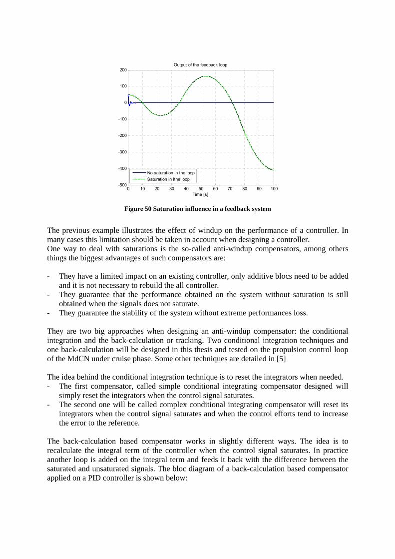
0 10 20 30 40 50 60 70 80 90 100-500
-400
-300
-200
-100
0
100
200Output of the feedback loop
Time [s]
No saturation in the loopSaturation in lthe loop
Figure 50 Saturation influence in a feedback system
The previous example illustrates the effect of windup on the performance of a controller. In many cases this limitation should be taken in account when designing a controller. One way to deal with saturations is the so-called anti-windup compensators, among others things the biggest advantages of such compensators are: - They have a limited impact on an existing controller, only additive blocs need to be added
and it is not necessary to rebuild the all controller. - They guarantee that the performance obtained on the system without saturation is still
obtained when the signals does not saturate. - They guarantee the stability of the system without extreme performances loss. They are two big approaches when designing an anti-windup compensator: the conditional integration and the back-calculation or tracking. Two conditional integration techniques and one back-calculation will be designed in this thesis and tested on the propulsion control loop of the MdCN under cruise phase. Some other techniques are detailed in [5] The idea behind the conditional integration technique is to reset the integrators when needed. - The first compensator, called simple conditional integrating compensator designed will
simply reset the integrators when the control signal saturates. - The second one will be called complex conditional integrating compensator will reset its
integrators when the control signal saturates and when the control efforts tend to increase the error to the reference.
The back-calculation based compensator works in slightly different ways. The idea is to recalculate the integral term of the controller when the control signal saturates. In practice another loop is added on the integral term and feeds it back with the difference between the saturated and unsaturated signals. The bloc diagram of a back-calculation based compensator applied on a PID controller is shown below:
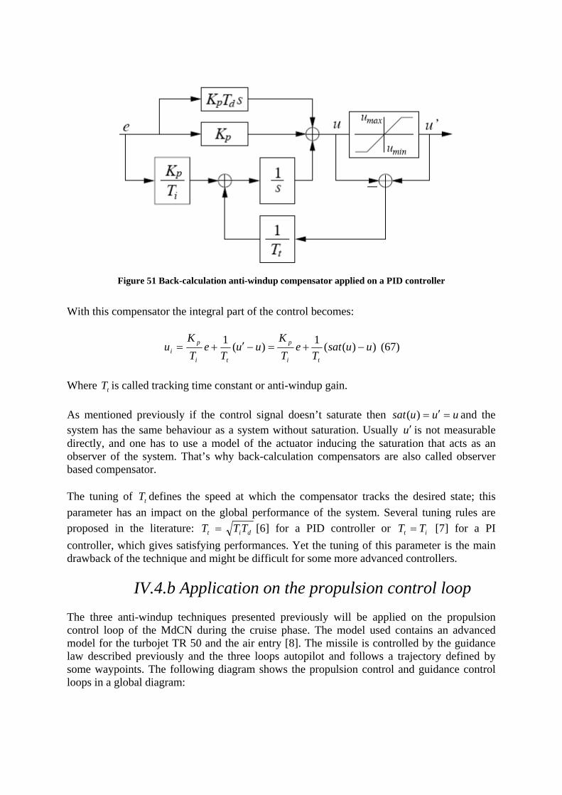
Figure 51 Back-calculation anti-windup compensator applied on a PID controller
With this compensator the integral part of the control becomes:
))((1)(1 uusatT
eTK
uuT
eTK
uti
p
ti
pi −+=−′+= (67)
Where tT is called tracking time constant or anti-windup gain. As mentioned previously if the control signal doesn’t saturate then uuusat =′=)( and the system has the same behaviour as a system without saturation. Usually u′ is not measurable directly, and one has to use a model of the actuator inducing the saturation that acts as an observer of the system. That’s why back-calculation compensators are also called observer based compensator. The tuning of tT defines the speed at which the compensator tracks the desired state; this parameter has an impact on the global performance of the system. Several tuning rules are proposed in the literature: dit TTT = [6] for a PID controller or it TT = [7] for a PI controller, which gives satisfying performances. Yet the tuning of this parameter is the main drawback of the technique and might be difficult for some more advanced controllers.
IV.4.b Application on the propulsion control loop The three anti-windup techniques presented previously will be applied on the propulsion control loop of the MdCN during the cruise phase. The model used contains an advanced model for the turbojet TR 50 and the air entry [8]. The missile is controlled by the guidance law described previously and the three loops autopilot and follows a trajectory defined by some waypoints. The following diagram shows the propulsion control and guidance control loops in a global diagram:
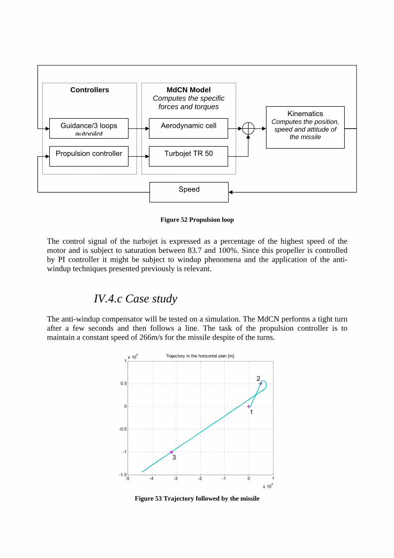
Figure 52 Propulsion loop
The control signal of the turbojet is expressed as a percentage of the highest speed of the motor and is subject to saturation between 83.7 and 100%. Since this propeller is controlled by PI controller it might be subject to windup phenomena and the application of the anti-windup techniques presented previously is relevant.
IV.4.c Case study The anti-windup compensator will be tested on a simulation. The MdCN performs a tight turn after a few seconds and then follows a line. The task of the propulsion controller is to maintain a constant speed of 266m/s for the missile despite of the turns.
-5 -4 -3 -2 -1 0 1
x 104
-1.5
-1
-0.5
0
0.5
1x 10⁴
1
2
3
Trajectory in the horizontal plan [m]
Figure 53 Trajectory followed by the missile
MdCN Model Computes the specific
forces and torques
Controllers
Guidance/3 loops autopilot
Aerodynamic cell
Turbojet TR 50 Propulsion controller
Kinematics Computes the position, speed and attitude of
the missile
Speed
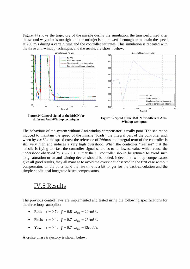
Figure 44 shows the trajectory of the missile during the simulation, the turn performed after the second waypoint is too tight and the turbojet is not powerful enough to maintain the speed at 266 m/s during a certain time and the controller saturates. This simulation is repeated with the three anti-windup techniques and the results are shown below:
0 50 100 150 200 25082
84
86
88
90
92
94
96
98
100
Time [s]
Control signals [% rpm]
No AWBack-calculationSimple conditionnal integrationComplex conditionnal integration
Figure 54 Control signal of the MdCN for
different Anti-Windup techniques
0 50 100 150 200 250180
200
220
240
260
280
300
320
340
Time [s]
Speed of the missile [m/s]
No AWBack-calculationSimple conditionnal integrationComplex conditionnal integration
Figure 55 Speed of the MdCN for different Anti-
Windup techiques The behaviour of the system without Anti-windup compensator is really poor. The saturation induced to maintain the speed of the missile “loads” the integral part of the controller and, when by st 60≈ the speed cross the reference of 266m/s, the integral term of the controller is still very high and induces a very high overshoot. When the controller “realises” that the missile is flying too fast the controller signal saturates to its lowest value which cause the undershoot observed by st 200≈ . Either the PI controller should be retuned to avoid such long saturation or an anti-windup device should be added. Indeed anti-windup compensators give all good results, they all manage to avoid the overshoot observed in the first case without compensator, on the other hand the rise time is a bit longer for the back-calculation and the simple conditional integrator based compensators.
IV.5 Results The previous control laws are implemented and tested using the following specifications for the three loops autopilot:
• Roll: srads CR /208.07.0 === ωξτ
• Pitch: srads CR /257.04.0 === ωξτ
• Yaw: srads CR /127.04.0 === ωξτ A cruise phase trajectory is shown below:
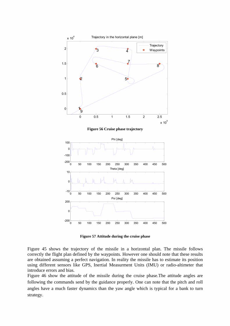
0 0.5 1 1.5 2 2.5
x 104
0
0.5
1
1.5
2
x 104
1
2
3 4
5
67
8
9
Trajectory in the horizontal plane [m]
TrajectoryWaypoints
Figure 56 Cruise phase trajectory
0 50 100 150 200 250 300 350 400 450 500-200
-100
0
100Phi [deg]
0 50 100 150 200 250 300 350 400 450 500-10
0
10Theta [deg]
0 50 100 150 200 250 300 350 400 450 500-200
0
200Psi [deg]
Figure 57 Attitude during the cruise phase
Figure 45 shows the trajectory of the missile in a horizontal plan. The missile follows correctly the flight plan defined by the waypoints. However one should note that these results are obtained assuming a perfect navigation. In reality the missile has to estimate its position using different sensors like GPS, Inertial Measurment Units (IMU) or radio-altimeter that introduce errors and bias. Figure 46 show the attitude of the missile during the cruise phase.The attitude angles are following the commands send by the guidance properly. One can note that the pitch and roll angles have a much faster dynamics than the yaw angle which is typical for a bank to turn strategy.
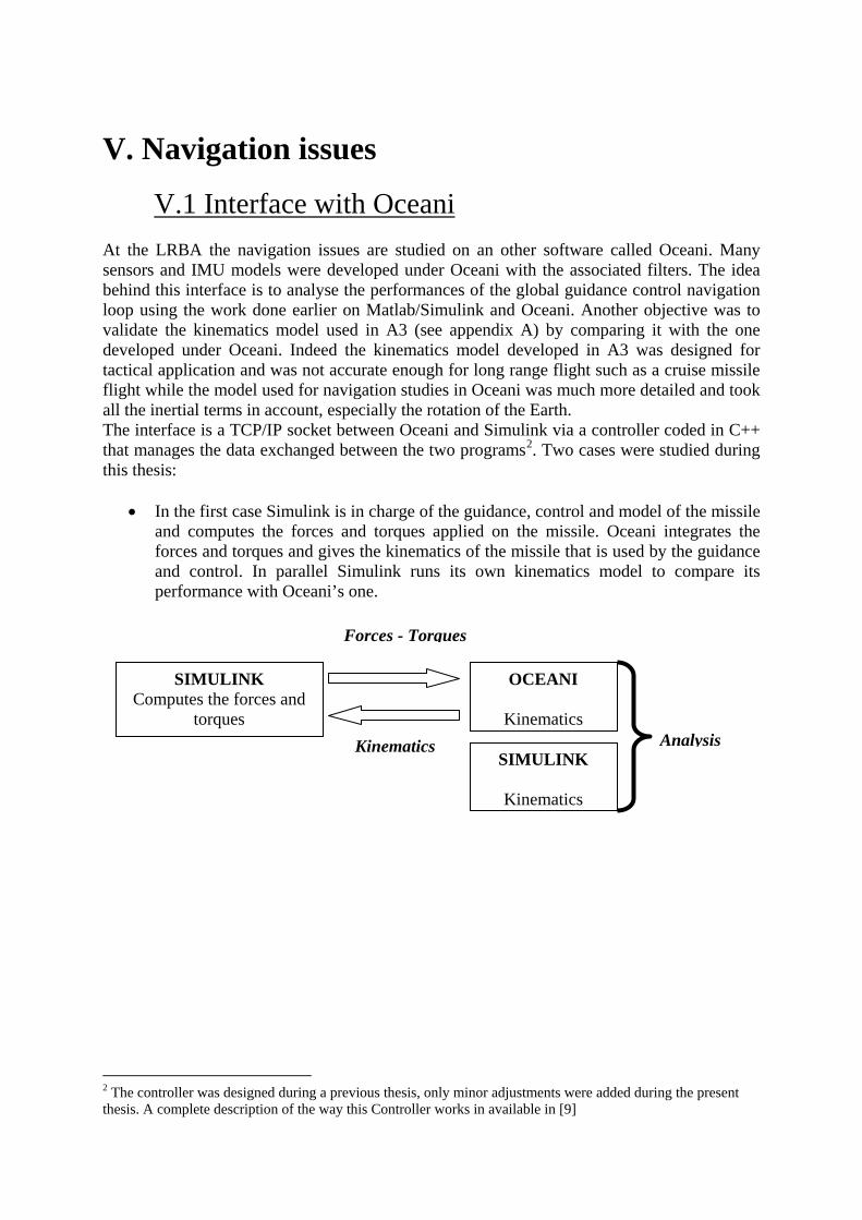
V. Navigation issues
V.1 Interface with Oceani At the LRBA the navigation issues are studied on an other software called Oceani. Many sensors and IMU models were developed under Oceani with the associated filters. The idea behind this interface is to analyse the performances of the global guidance control navigation loop using the work done earlier on Matlab/Simulink and Oceani. Another objective was to validate the kinematics model used in A3 (see appendix A) by comparing it with the one developed under Oceani. Indeed the kinematics model developed in A3 was designed for tactical application and was not accurate enough for long range flight such as a cruise missile flight while the model used for navigation studies in Oceani was much more detailed and took all the inertial terms in account, especially the rotation of the Earth. The interface is a TCP/IP socket between Oceani and Simulink via a controller coded in C++ that manages the data exchanged between the two programs2. Two cases were studied during this thesis:
• In the first case Simulink is in charge of the guidance, control and model of the missile and computes the forces and torques applied on the missile. Oceani integrates the forces and torques and gives the kinematics of the missile that is used by the guidance and control. In parallel Simulink runs its own kinematics model to compare its performance with Oceani’s one.
2 The controller was designed during a previous thesis, only minor adjustments were added during the present thesis. A complete description of the way this Controller works in available in [9]
OCEANI
Kinematics
SIMULINK Computes the forces and
torques
SIMULINK
Kinematics
AnalysisKinematics
Forces - Torques
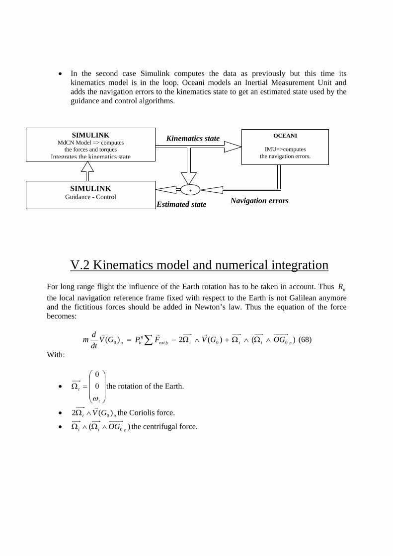
• In the second case Simulink computes the data as previously but this time its
kinematics model is in the loop. Oceani models an Inertial Measurement Unit and adds the navigation errors to the kinematics state to get an estimated state used by the guidance and control algorithms.
V.2 Kinematics model and numerical integration
For long range flight the influence of the Earth rotation has to be taken in account. Thus nR the local navigation reference frame fixed with respect to the Earth is not Galilean anymore and the fictitious forces should be added in Newton’s law. Thus the equation of the force becomes:
)()(2)( 000 ntttbextn
bn OGGVFPGVdtdm ∧Ω∧Ω+∧Ω−= ∑
rrr (68)
With:
• ⎟⎟⎟
⎠
⎞
⎜⎜⎜
⎝
⎛=Ω
t
t
ω00
the rotation of the Earth.
• nt GV )(2 0
r∧Ω the Coriolis force.
• )( 0 ntt OG∧Ω∧Ω the centrifugal force.
Kinematics state SIMULINK MdCN Model => computes
the forces and torques Integrates the kinematics state
OCEANI
IMU=>computes the navigation errors.
+SIMULINK Guidance - Control Navigation errors Estimated state
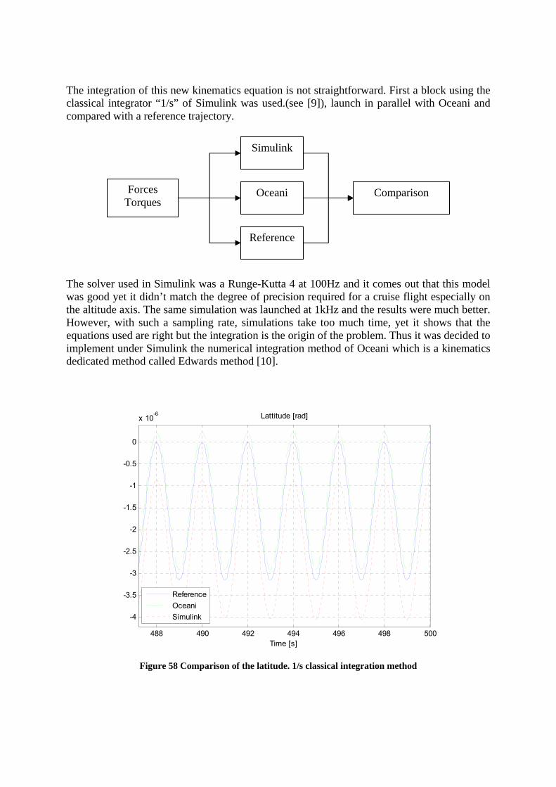
The integration of this new kinematics equation is not straightforward. First a block using the classical integrator “1/s” of Simulink was used.(see [9]), launch in parallel with Oceani and compared with a reference trajectory. The solver used in Simulink was a Runge-Kutta 4 at 100Hz and it comes out that this model was good yet it didn’t match the degree of precision required for a cruise flight especially on the altitude axis. The same simulation was launched at 1kHz and the results were much better. However, with such a sampling rate, simulations take too much time, yet it shows that the equations used are right but the integration is the origin of the problem. Thus it was decided to implement under Simulink the numerical integration method of Oceani which is a kinematics dedicated method called Edwards method [10].
488 490 492 494 496 498 500
-4
-3.5
-3
-2.5
-2
-1.5
-1
-0.5
0
x 10-6 Lattitude [rad]
Time [s]
ReferenceOceaniSimulink
Figure 58 Comparison of the latitude. 1/s classical integration method
Forces Torques
Simulink
Oceani
Reference
Comparison
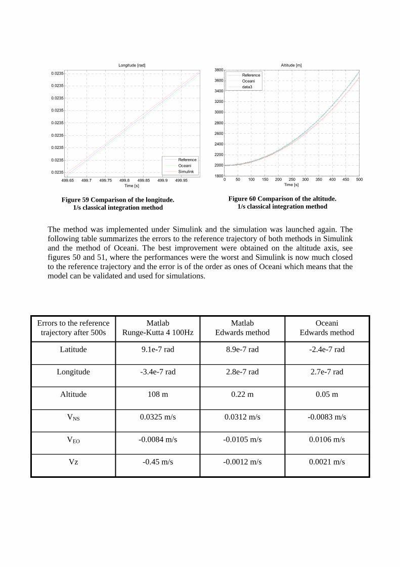
499.65 499.7 499.75 499.8 499.85 499.9 499.95
0.0235
0.0235
0.0235
0.0235
0.0235
0.0235
0.0235
0.0235
0.0235
Longitude [rad]
Time [s]
ReferenceOceaniSimulink
Figure 59 Comparison of the longitude.
1/s classical integration method
0 50 100 150 200 250 300 350 400 450 5001800
2000
2200
2400
2600
2800
3000
3200
3400
3600
3800Altitude [m]
Time [s]
ReferenceOceanidata3
Figure 60 Comparison of the altitude.
1/s classical integration method
The method was implemented under Simulink and the simulation was launched again. The following table summarizes the errors to the reference trajectory of both methods in Simulink and the method of Oceani. The best improvement were obtained on the altitude axis, see figures 50 and 51, where the performances were the worst and Simulink is now much closed to the reference trajectory and the error is of the order as ones of Oceani which means that the model can be validated and used for simulations.
-0.45 m/s
-0.0084 m/s
0.0325 m/s
108 m
-3.4e-7 rad
9.1e-7 rad
Matlab Runge-Kutta 4 100Hz
0.0021 m/s -0.0012 m/s Vz
0.0106 m/s -0.0105 m/s VEO
-0.0083 m/s 0.0312 m/s VNS
0.05 m 0.22 m Altitude
2.7e-7 rad 2.8e-7 rad Longitude
-2.4e-7 rad 8.9e-7 rad Latitude
Oceani Edwards method
Matlab Edwards method
Errors to the reference trajectory after 500s
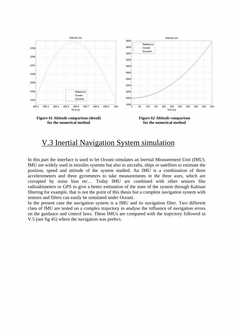
499.2 499.3 499.4 499.5 499.6 499.7 499.8 499.9 500
3763
3764
3765
3766
3767
3768
3769
Altitude [m]
Time [s]
ReferenceOceaniSimulink
Figure 61 Altitude comparison (detail)
for the numerical method
0 50 100 150 200 250 300 350 400 450 5001800
2000
2200
2400
2600
2800
3000
3200
3400
3600
3800Altitude [m]
Time [s]
ReferenceOceaniSimulink
Figure 62 Altitude comparison
for the numerical method
V.3 Inertial Navigation System simulation In this part the interface is used to let Oceani simulates an Inertial Measurement Unit (IMU). IMU are widely used in missiles systems but also in aircrafts, ships or satellites to estimate the position, speed and attitude of the system studied. An IMU is a combination of three accelerometers and three gyrometers to take measurements in the three axes, which are corrupted by noise bias etc… Today IMU are combined with other sensors like radioaltimeters or GPS to give a better estimation of the state of the system through Kalman filtering for example, that is not the point of this thesis but a complete navigation system with sensors and filters can easily be simulated under Oceani. In the present case the navigation system is a IMU and its navigation filter. Two different class of IMU are tested on a complex trajectory to analyse the influence of navigation errors on the guidance and control laws. These IMUs are compared with the trajectory followed in V.5 (see fig 45) where the navigation was perfect.
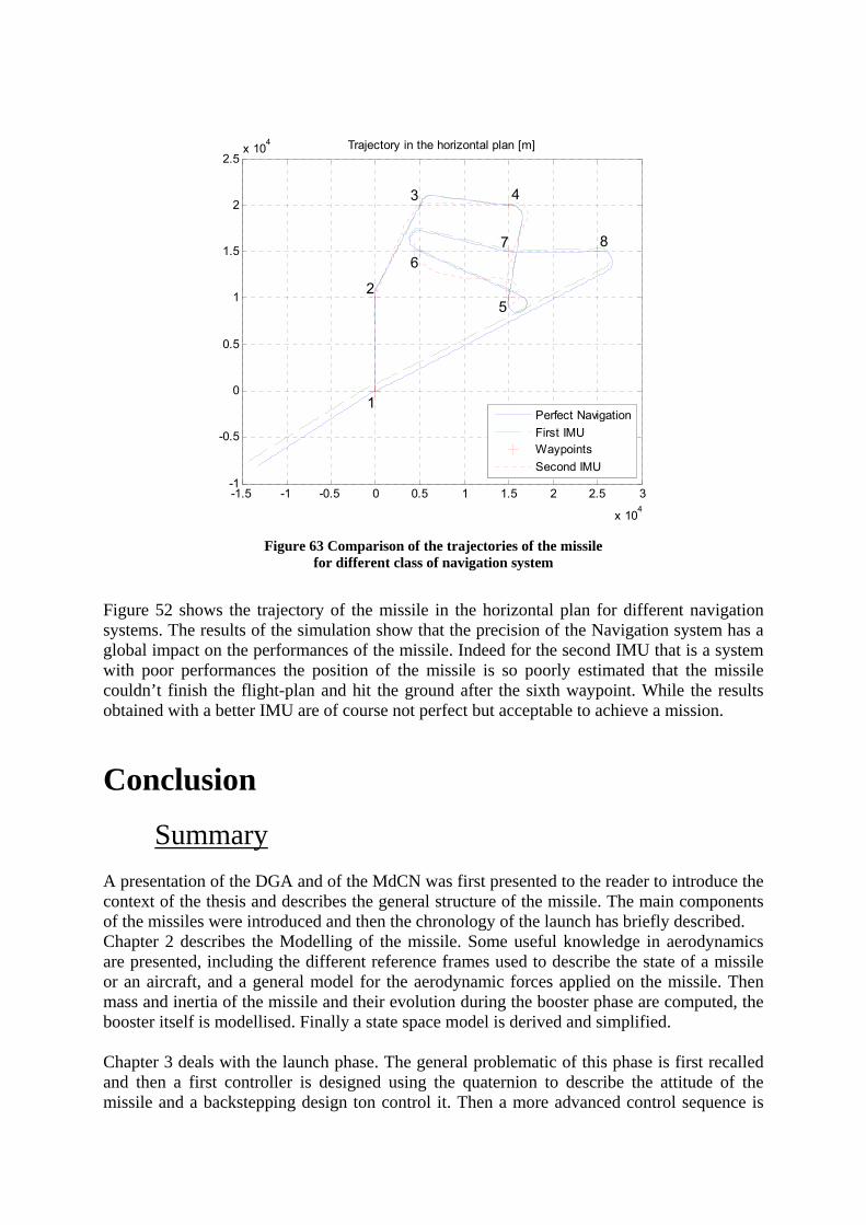
-1.5 -1 -0.5 0 0.5 1 1.5 2 2.5 3
x 104
-1
-0.5
0
0.5
1
1.5
2
2.5x 10⁴
1
2
3 4
5
67 8
Trajectory in the horizontal plan [m]
Perfect NavigationFirst IMUWaypointsSecond IMU
Figure 63 Comparison of the trajectories of the missile
for different class of navigation system
Figure 52 shows the trajectory of the missile in the horizontal plan for different navigation systems. The results of the simulation show that the precision of the Navigation system has a global impact on the performances of the missile. Indeed for the second IMU that is a system with poor performances the position of the missile is so poorly estimated that the missile couldn’t finish the flight-plan and hit the ground after the sixth waypoint. While the results obtained with a better IMU are of course not perfect but acceptable to achieve a mission.
Conclusion
Summary A presentation of the DGA and of the MdCN was first presented to the reader to introduce the context of the thesis and describes the general structure of the missile. The main components of the missiles were introduced and then the chronology of the launch has briefly described. Chapter 2 describes the Modelling of the missile. Some useful knowledge in aerodynamics are presented, including the different reference frames used to describe the state of a missile or an aircraft, and a general model for the aerodynamic forces applied on the missile. Then mass and inertia of the missile and their evolution during the booster phase are computed, the booster itself is modellised. Finally a state space model is derived and simplified. Chapter 3 deals with the launch phase. The general problematic of this phase is first recalled and then a first controller is designed using the quaternion to describe the attitude of the missile and a backstepping design ton control it. Then a more advanced control sequence is
introduced to match the specifications needed to ignite properly the booster. Based on the same controller an AoA and sideslip compensator is designed and finally the parameters of the control sequence are chosen using a statistic analysis. In a last part the performances of the controller designed are analysed for different conditions, it came out the backstepping based controller could give good results under many conditions Chapter 4 describes the cruise phase issue. To analyse the performances of different anti-windup compensators on the propulsion control loop a guidance control algorithm is briefly described and implemented, then the windup phenomenon is introduced and the two main anti-windup techniques are briefly presented and finally tested on a case study. The results of this analysis were that saturations have to be taken in account when designing the controllers and that the different anti-windup techniques gave comparable and satisfying results. Chapter 5 presents the work done to take the navigation errors in account in the control guidance algorithms. Matlab/Simulink is interfaced with a navigation software called Oceani A new kinematics model for Smulink is derived based on a comparison with Oceani’s one and a reference trajectory and finally a IMU simulated by Oceani is introduced in the loop to add some navigation errors to the state. Different types of IMU are compared with the results obtained with a perfect navigation. It came out that navigation errors can lead to the crash of the missile and that a simple IMU was not enough for a cruise flight.
Future works There are several possible improvement of the work presented here, some of them are given here as future possible works:
• The robustness of the Backstepping controller to model errors should be analysed. This will be more instructive when the design of the MdCN will be a bit more advanced and when the DGA will have a better idea of the model of the missile.
• A study can be lead to analyse the influence of the waves and the sea on the attitude of the carrier and thus on the initial position of the MdCN to see whether or not the missile can be fired when the sea conditions are bad.
• The backstepping controller could be compared with a classical linear controller to see
if the non-linear techniques improve the performance, availability and reliability of the missile.
• Concerning the anti-windup compensator applied on the propulsion loop, it could be interesting to study the fuel consumption induced by the different compensators and to study their impact on the global range of the missile.
• More advanced navigation system should be introduced in the loop using different sensors like GPS or radioaltimeter hybridised with the IMU and the corresponding filters to simulate a navigation system closer to the one that will be used in the MdCN.
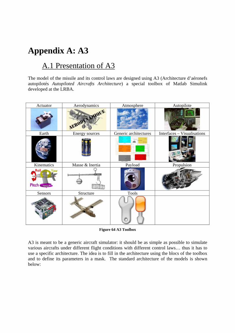
Appendix A: A3
A.1 Presentation of A3 The model of the missile and its control laws are designed using A3 (Architecture d’aéronefs autopilotés Autopiloted Aircrafts Architecture) a special toolbox of Matlab Simulink developed at the LRBA.
Actuator Aerodynamics Atmosphere Autopilote
Earth Energy sources Generic architectures Interfaces – Visualisations
Kinematics Masse & Inertia Payload Propulsion
Sensors Structure Tools
Figure 64 A3 Toolbox
A3 is meant to be a generic aircraft simulator: it should be as simple as possible to simulate various aircrafts under different flight conditions with different control laws… thus it has to use a specific architecture. The idea is to fill in the architecture using the blocs of the toolbox and to define its parameters in a mask. The standard architecture of the models is shown below:
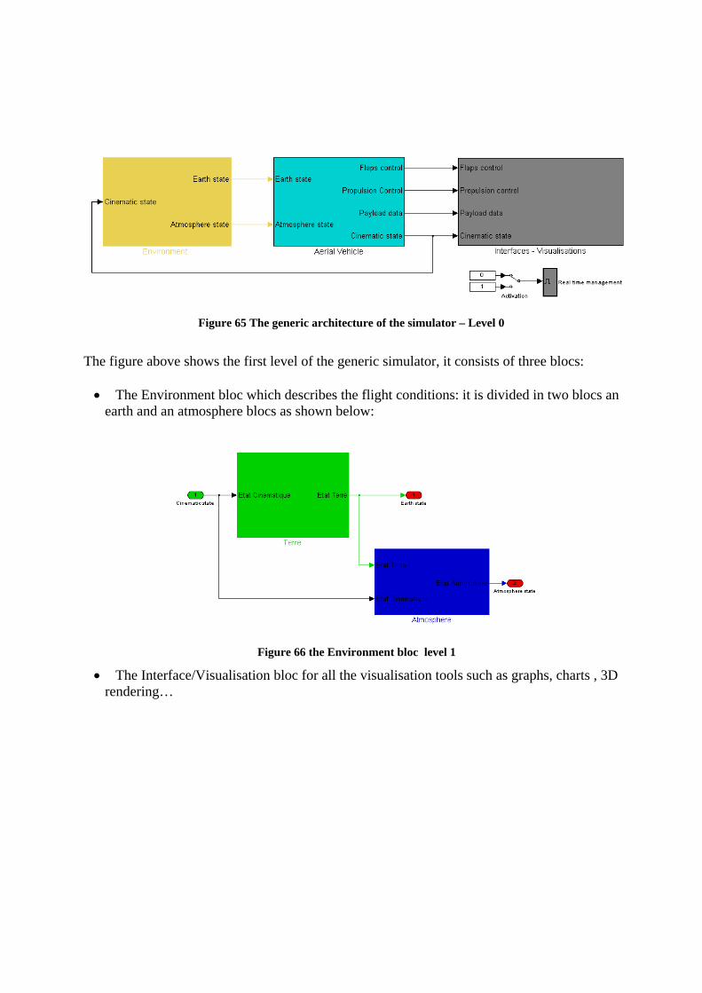
Figure 65 The generic architecture of the simulator – Level 0
The figure above shows the first level of the generic simulator, it consists of three blocs:
• The Environment bloc which describes the flight conditions: it is divided in two blocs an earth and an atmosphere blocs as shown below:
Figure 66 the Environment bloc level 1
• The Interface/Visualisation bloc for all the visualisation tools such as graphs, charts , 3D rendering…
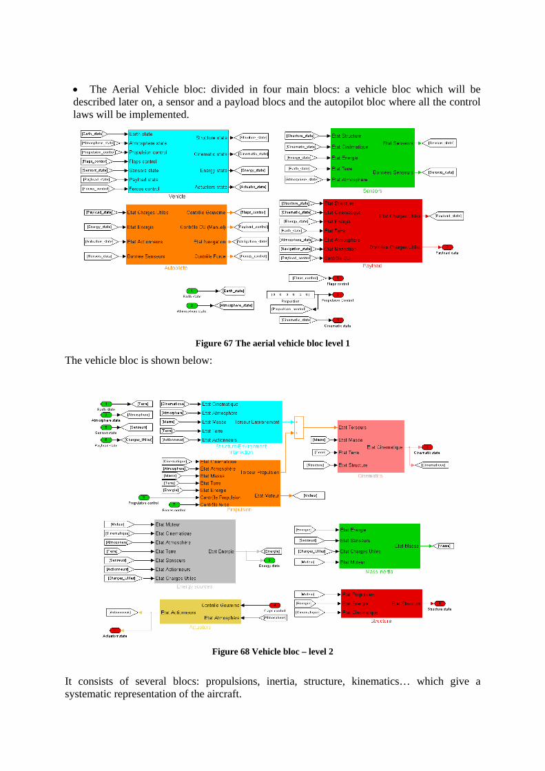
• The Aerial Vehicle bloc: divided in four main blocs: a vehicle bloc which will be described later on, a sensor and a payload blocs and the autopilot bloc where all the control laws will be implemented.
Figure 67 The aerial vehicle bloc level 1
The vehicle bloc is shown below:
Figure 68 Vehicle bloc – level 2
It consists of several blocs: propulsions, inertia, structure, kinematics… which give a systematic representation of the aircraft.
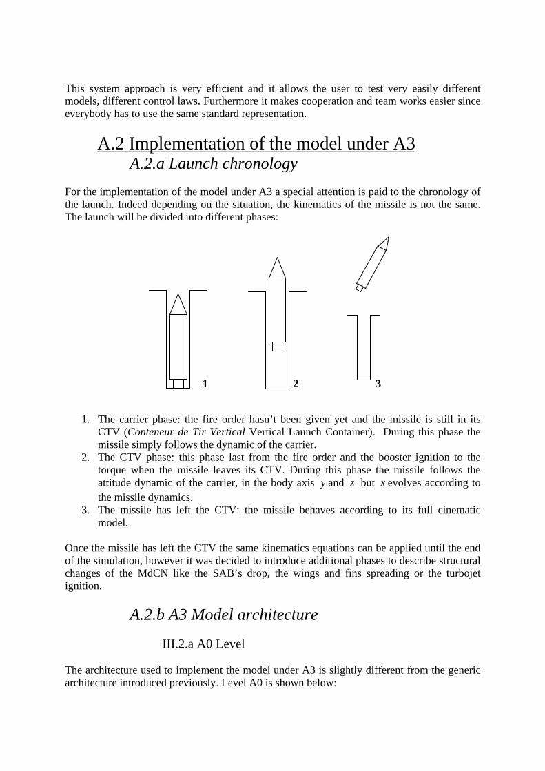
This system approach is very efficient and it allows the user to test very easily different models, different control laws. Furthermore it makes cooperation and team works easier since everybody has to use the same standard representation.
A.2 Implementation of the model under A3 A.2.a Launch chronology
For the implementation of the model under A3 a special attention is paid to the chronology of the launch. Indeed depending on the situation, the kinematics of the missile is not the same. The launch will be divided into different phases:
1. The carrier phase: the fire order hasn’t been given yet and the missile is still in its CTV (Conteneur de Tir Vertical Vertical Launch Container). During this phase the missile simply follows the dynamic of the carrier.
2. The CTV phase: this phase last from the fire order and the booster ignition to the torque when the missile leaves its CTV. During this phase the missile follows the attitude dynamic of the carrier, in the body axis y and z but x evolves according to the missile dynamics.
3. The missile has left the CTV: the missile behaves according to its full cinematic model.
Once the missile has left the CTV the same kinematics equations can be applied until the end of the simulation, however it was decided to introduce additional phases to describe structural changes of the MdCN like the SAB’s drop, the wings and fins spreading or the turbojet ignition.
A.2.b A3 Model architecture
III.2.a A0 Level The architecture used to implement the model under A3 is slightly different from the generic architecture introduced previously. Level A0 is shown below:
1 2 3
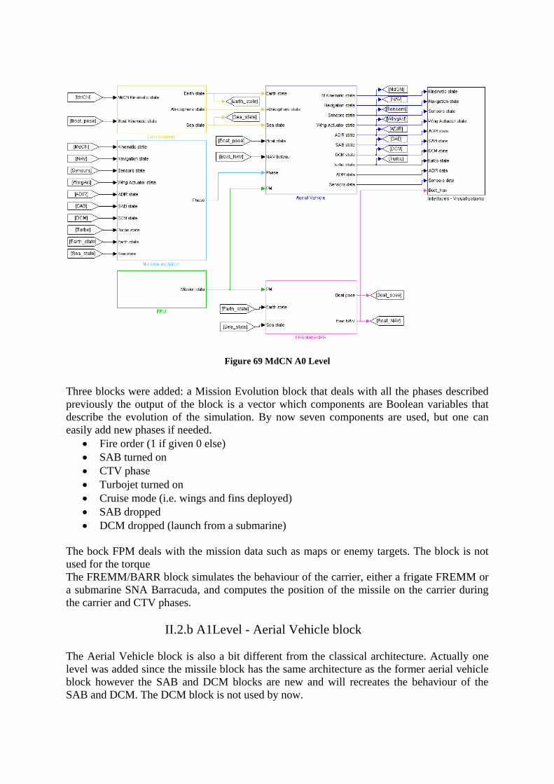
Figure 69 MdCN A0 Level
Three blocks were added: a Mission Evolution block that deals with all the phases described previously the output of the block is a vector which components are Boolean variables that describe the evolution of the simulation. By now seven components are used, but one can easily add new phases if needed.
• Fire order (1 if given 0 else) • SAB turned on • CTV phase • Turbojet turned on • Cruise mode (i.e. wings and fins deployed) • SAB dropped • DCM dropped (launch from a submarine)
The bock FPM deals with the mission data such as maps or enemy targets. The block is not used for the torque The FREMM/BARR block simulates the behaviour of the carrier, either a frigate FREMM or a submarine SNA Barracuda, and computes the position of the missile on the carrier during the carrier and CTV phases.
II.2.b A1Level - Aerial Vehicle block The Aerial Vehicle block is also a bit different from the classical architecture. Actually one level was added since the missile block has the same architecture as the former aerial vehicle block however the SAB and DCM blocks are new and will recreates the behaviour of the SAB and DCM. The DCM block is not used by now.
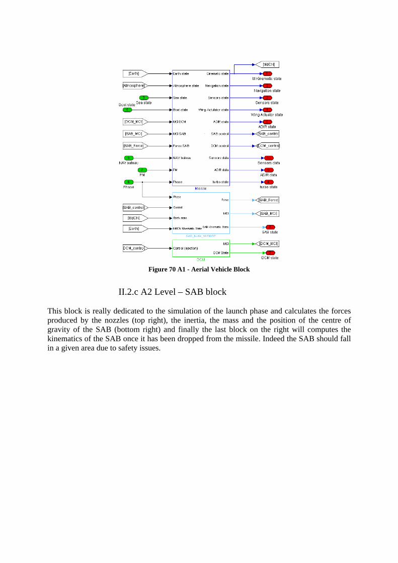
Figure 70 A1 - Aerial Vehicle Block
II.2.c A2 Level – SAB block
This block is really dedicated to the simulation of the launch phase and calculates the forces produced by the nozzles (top right), the inertia, the mass and the position of the centre of gravity of the SAB (bottom right) and finally the last block on the right will computes the kinematics of the SAB once it has been dropped from the missile. Indeed the SAB should fall in a given area due to safety issues.
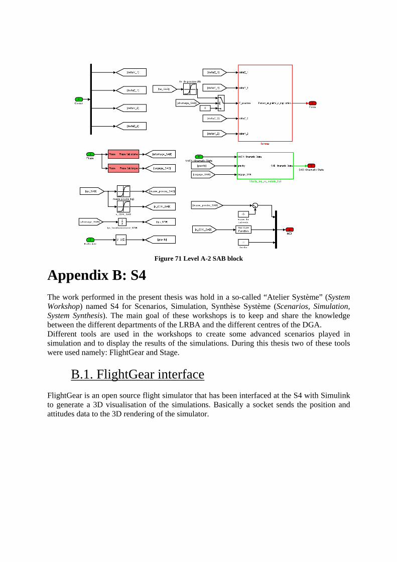
Figure 71 Level A-2 SAB block
Appendix B: S4 The work performed in the present thesis was hold in a so-called “Atelier Système” (System Workshop) named S4 for Scenarios, Simulation, Synthèse Système (Scenarios, Simulation, System Synthesis). The main goal of these workshops is to keep and share the knowledge between the different departments of the LRBA and the different centres of the DGA. Different tools are used in the workshops to create some advanced scenarios played in simulation and to display the results of the simulations. During this thesis two of these tools were used namely: FlightGear and Stage.
B.1. FlightGear interface FlightGear is an open source flight simulator that has been interfaced at the S4 with Simulink to generate a 3D visualisation of the simulations. Basically a socket sends the position and attitudes data to the 3D rendering of the simulator.
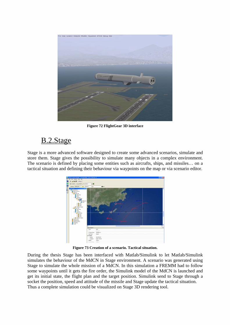
Figure 72 FlightGear 3D interface
B.2.Stage Stage is a more advanced software designed to create some advanced scenarios, simulate and store them. Stage gives the possibility to simulate many objects in a complex environment. The scenario is defined by placing some entities such as aircrafts, ships, and missiles… on a tactical situation and defining their behaviour via waypoints on the map or via scenario editor.
Figure 73 Creation of a scenario. Tactical situation.
During the thesis Stage has been interfaced with Matlab/Simulink to let Matlab/Simulink simulates the behaviour of the MdCN in Stage environment. A scenario was generated using Stage to simulate the whole mission of a MdCN. In this simulation a FREMM had to follow some waypoints until it gets the fire order, the Simulink model of the MdCN is launched and get its initial state, the flight plan and the target position. Simulink send to Stage through a socket the position, speed and attitude of the missile and Stage update the tactical situation. Thus a complete simulation could be visualized on Stage 3D rendering tool.
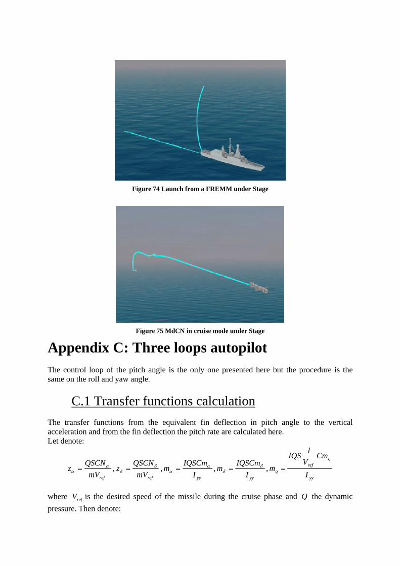
Figure 74 Launch from a FREMM under Stage
Figure 75 MdCN in cruise mode under Stage
Appendix C: Three loops autopilot The control loop of the pitch angle is the only one presented here but the procedure is the same on the roll and yaw angle.
C.1 Transfer functions calculation The transfer functions from the equivalent fin deflection in pitch angle to the vertical acceleration and from the fin deflection the pitch rate are calculated here. Let denote:
refmVQSCN
z αα = ,
refmVQSCN
z δδ = ,
yyIIQSCm
m αα = ,
yyIIQSCm
m δδ = ,
yy
qref
q I
CmV
lIQSm =
where refV is the desired speed of the missile during the cruise phase and Q the dynamic pressure. Then denote:
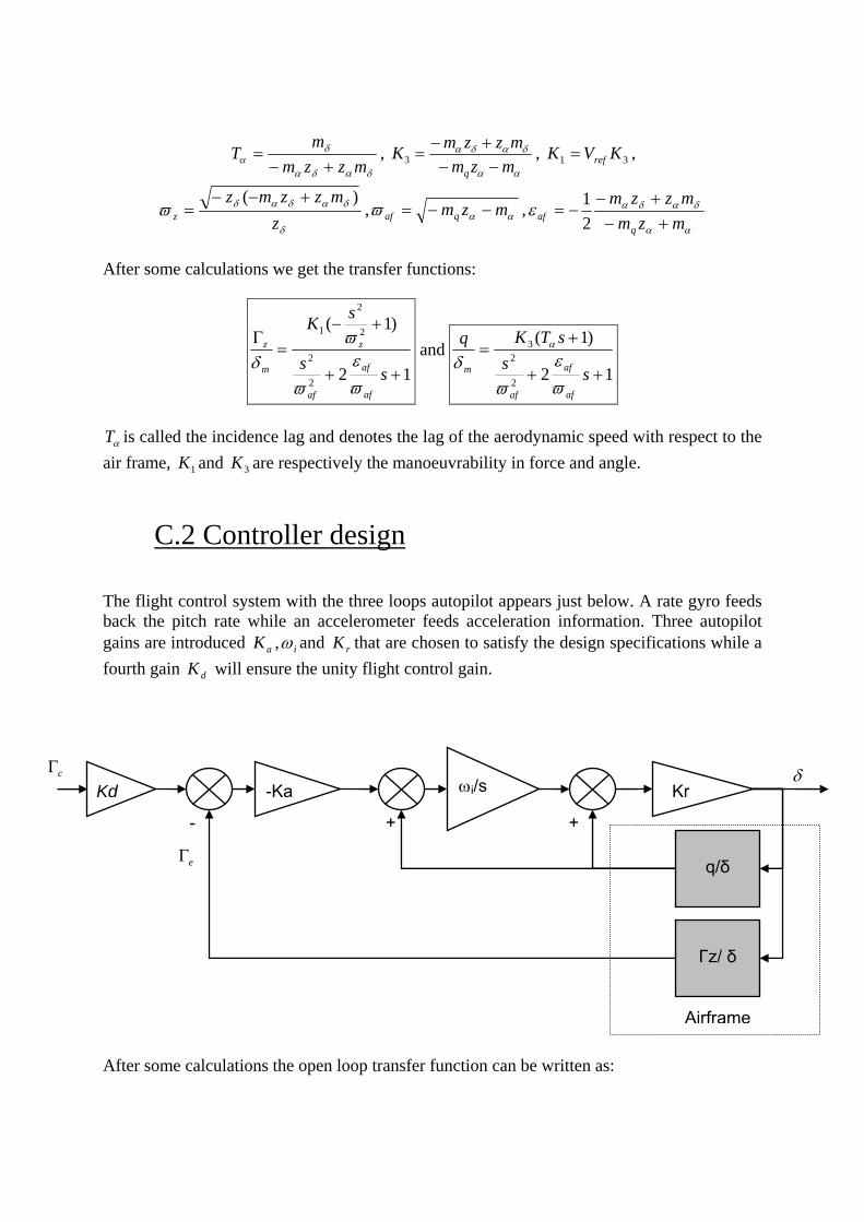
δαδα
δα mzzm
mT
+−= ,
αα
δαδα
mzmmzzmK
q −−+−
=3 , 31 KVK ref= ,
δ
δαδαδϖz
mzzmzz
)( +−−= , ααϖ mzmqaf −−= ,
αα
δαδαεmzm
mzzm
qaf +−
+−−=
21
After some calculations we get the transfer functions:
12
)1(
2
2
2
2
1
++
+−=
Γ
ss
sK
af
af
af
z
m
z
ϖε
ϖ
ϖδ
and 12
)1(
2
23
++
+=
sssTKq
af
af
af
m
ϖε
ϖδ
α
αT is called the incidence lag and denotes the lag of the aerodynamic speed with respect to the
air frame, 1K and 3K are respectively the manoeuvrability in force and angle.
C.2 Controller design The flight control system with the three loops autopilot appears just below. A rate gyro feeds back the pitch rate while an accelerometer feeds acceleration information. Three autopilot gains are introduced aK , iω and rK that are chosen to satisfy the design specifications while a fourth gain dK will ensure the unity flight control gain.
After some calculations the open loop transfer function can be written as:
Airframe
-
Kd
Γz/ δ
q/δ
-Ka ωi/s Kr
+ +
cΓ
eΓ
δ
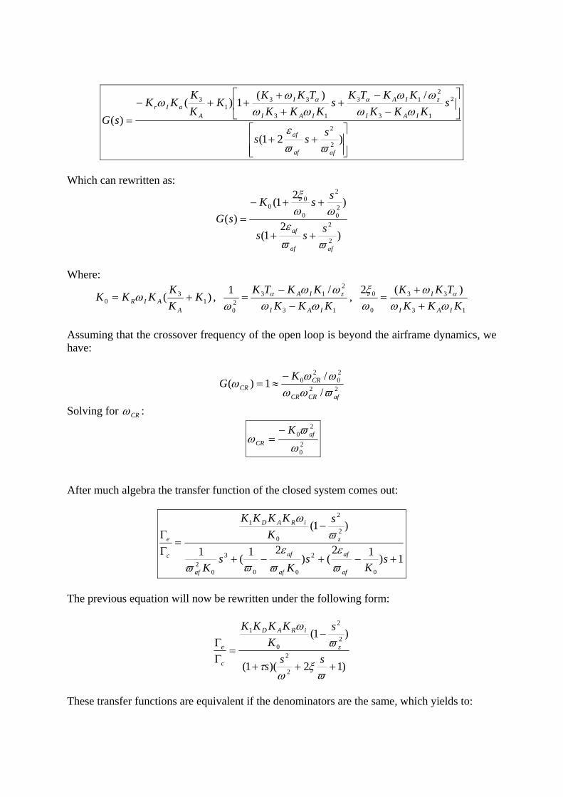
⎥⎥⎦
⎤
⎢⎢⎣
⎡++
⎥⎦
⎤⎢⎣
⎡−
−+
++
++−
=
)21(
/)(1)(
)(
2
2
2
13
213
13
331
3
afaf
af
IAI
zIA
IAI
I
AaIr
sss
sKKK
KKTKs
KKKTKK
KKK
KKsG
ϖϖε
ωωωω
ωωω
ω αα
Which can rewritten as:
)2
1(
)2
1()(
2
2
20
2
0
00
afaf
af sss
ssKsG
ϖϖε
ωωξ
++
++−=
Where:
)( 13
0 KKK
KKKA
AIR += ω , 13
213
20
/1KKK
KKTK
IAI
zIA
ωωωω
ωα
−−
= , 13
33
0
0 )(2KKK
TKK
IAI
I
ωωω
ωξ α
++
=
Assuming that the crossover frequency of the open loop is beyond the airframe dynamics, we have:
22
20
20
//
1)(afCRCR
CRCR
KG
ϖωωωω
ω−
≈=
Solving for CRω :
20
20
ωϖ
ω afCR
K−=
After much algebra the transfer function of the closed system comes out:
1)12()
21(1
)1(
0
2
00
3
02
2
2
0
1
+−+−+
−=
ΓΓ
sK
sK
sK
sK
KKKK
af
af
af
af
af
z
iRAD
c
e
ϖε
ϖε
ϖϖ
ϖω
The previous equation will now be rewritten under the following form:
)12)(1(
)1(
2
2
2
2
0
1
+++
−=
ΓΓ
ϖξ
ωτ
ϖω
sss
sK
KKKK
z
iRAD
c
e
These transfer functions are equivalent if the denominators are the same, which yields to:
022
1Kafϖω
τ−= ,
020
2
2121Kaf
af
ϖε
ϖωξτ
ω−=+ ,
00
0 122K
−=+ϖξ
τωξ
For a given airframe and given flight condition we know afϖ and afε . Thus if we specify a desired time constant τ , a desired damping ξ for the closed loop system and a desired
crossover frequency CRω for the open loop system, we have four unknowns left 00 ,, ωξω and 0K which are directly linked to the autopilot gain. Recalling the equation for CRω derived from the open loop analysis we have the following system of four equations and four unknowns:
0
22
1Kafϖω
τ−= ,
020
2
2121Kaf
af
ϖε
ϖωξτ
ω−=+ ,
00
0 122K
−=+ϖξ
τωξ , 2
0
20
ωϖ
ω afCR
K−=
Which can be solved for the autopilot gains and we finally get the following expressions:
22000
002
20
21
21
αα
α
ωωξ
ωξϖω
TT
TK z
C +−
+−−= and
CD KK += 1 1
3
KKK
KC
A =
2
20
20
1z
C
CI
K
KT
ϖω
ωω α
++=
IADr KKK
KK
ω1
0=
Figure table
Figure 1 Air Picture of the LRBA ............................................................................................ 10 Figure 2 MdCN prototype with its SAB at the bottom Note the two swivelling nozzles ........ 12 Figure 3 General structure of the MdCN ................................................................................. 13 Figure 4 Launch from a FREMM ............................................................................................ 13 Figure 5 Launch from a submarine .......................................................................................... 14 Figure 6Earth reference system ................................................................................................ 16 Figure 7 Roll angle ................................................................................................................... 17 Figure 8 Pitch angle .................................................................................................................. 17 Figure 9 Yaw angle .................................................................................................................. 17 Figure 10 Rotation from R0 to Rb ........................................................................................... 18 Figure 11 Rotation from Rb to Ra ............................................................................................ 20 Figure 12 Rotation from R0 to Ra ............................................................................................ 21 Figure 13 Aerodynamic model ................................................................................................. 23 Figure 14 Mass of the booster during the launch phase ........................................................... 23 Figure 15 Nozzle cone of evolution ......................................................................................... 27 Figure 16 Guidance Control Navigation loop .......................................................................... 32 Figure 17 Pitch angle of the MdCN for different values of the reference slope ...................... 39 Figure 18 Angle of Attack (AoA of the MdCN for different values of the reference slope .... 39 Figure 19 Altitude of the MdCN for different values of the reference slope ........................... 39 Figure 20 Range of the MdCN for different values of the reference slope .............................. 39 Figure 21 Speed of the MdCN for different values of the reference slope .............................. 39 Figure 22 Desired Pitch angle .................................................................................................. 40 Figure 23 Relation between the pitch and AoA angles for a longitudinal flight ..................... 41 Figure 24 Distances to the optimal trajectory .......................................................................... 43 Figure 25 Desired pitch angle for all the sets tested ............................................................... 44 Figure 26 Desired pitch angle for the acceptable sets The best choice is shown in black ...... 44 Figure 27 Altitude of the missile for all the sets tested ........................................................... 44 Figure 28 Altitude of the missile for the acceptable sets ........................................................ 44 Figure 29 3D trajectories of the acceptable set of parameters. ................................................ 45 Figure 30 Sideslip angle for the acceptable sets. The best choice is shown in black ............ 46 Figure 31 AoA for the acceptable sets. The best choice is shown in black ............................ 46 Figure 32 Speed for the acceptable sets. .................................................................................. 47 Figure 33 Distance covered by the missile ............................................................................... 47 Figure 34 Pitch angle for the acceptable sets. The best set is shown in black and the
corresponding reference in blue. ...................................................................................... 47 Figure 35 Horizontal trajectories for the acceptable sets. The best set is shown in black. ...... 47 Figure 36 3D trajectories for different heading commands ..................................................... 48 Figure 37 Horizontal trajectories for different headings .......................................................... 48 Figure 38Altitude for different headings .................................................................................. 49 Figure 39 Speed for different headings .................................................................................... 49 Figure 40 Angle of Attack for different headings .................................................................... 49 Figure 41 Sideslip angle for different headings ....................................................................... 49 Figure 42 Influence of the carrier velocity on the altitude at the end of the booster phase ..... 50 Figure 43 Influence of the carrier velocity on the distance covered at the end of the booster
phase ................................................................................................................................. 50
Figure 44Influence of the carrier velocity on the speed of the missile at the end of the booster phase ................................................................................................................................. 50
Figure 45 Influence of the wind on the altitude ....................................................................... 51 Figure 46 Influence of the wind on the speed .......................................................................... 51 Figure 47 Influence of the wind on the Mach .......................................................................... 51 Figure 48 Mid-flight guidance ................................................................................................. 53 Figure 49 Bank to turn ............................................................................................................. 53 Figure 50 Saturation influence in a feedback system ............................................................... 55 Figure 51 Back-calculation anti-windup compensator applied on a PID controller ................ 56 Figure 52 Propulsion loop ........................................................................................................ 57 Figure 53 Trajectory followed by the missile .......................................................................... 57 Figure 54 Control signal of the MdCN for different Anti-Windup techniques ....................... 58 Figure 55 Speed of the MdCN for different Anti-Windup techiques ...................................... 58 Figure 56 Cruise phase trajectory ............................................................................................. 59 Figure 57 Attitude during the cruise phase .............................................................................. 59 Figure 58 Comparison of the latitude. 1/s classical integration method .................................. 62 Figure 59 Comparison of the longitude. 1/s classical integration method .............................. 63 Figure 60 Comparison of the altitude. 1/s classical integration method ................................. 63 Figure 61 Altitude comparison (detail) for the numerical method .......................................... 64 Figure 62 Altitude comparison for the numerical method ...................................................... 64 Figure 63 Comparison of the trajectories of the missile for different class of navigation
system ............................................................................................................................... 65 Figure 64 A3 Toolbox .............................................................................................................. 67 Figure 65 The generic architecture of the simulator – Level 0 ................................................ 68 Figure 66 the Environment bloc level 1 .................................................................................. 68 Figure 67 The aerial vehicle bloc level 1 ................................................................................. 69 Figure 68 Vehicle bloc – level 2 .............................................................................................. 69 Figure 69 MdCN A0 Level ...................................................................................................... 71 Figure 70 A1 - Aerial Vehicle Block ....................................................................................... 72 Figure 71 Level A-2 SAB block .............................................................................................. 73 Figure 72 FlightGear 3D interface ........................................................................................... 74 Figure 73 Creation of a scenario. Tactical situation. ................................................................ 74 Figure 74 Launch from a FREMM under Stage ...................................................................... 75 Figure 75 MdCN in cruise mode under Stage .......................................................................... 75
Bibliography [1] G. Taquin, Compendium in Flight Mechanics, SupAéro, pages 3-31, Sep. 2005
[2] Johnson, E. N. Limited Authority Adaptive Flight Control. PhD thesis, Georgia Institute of
Technology, School of Aerospace Engineering, Atlanta, GA 30332, Dec 2000.
[3] J.-P. Nouaille, Lecture notes in Guidage, internal formation LRBA, Oct. 2006
[4] P. Zarchan. Tactical and Strategic Three-Loop Autopilot, Tactical and Strategic Missile
Guidance, AIAAProgress in Astronautics and Aeronautics, volume 76, pages 507-515, 1997
[5] A. Visioli. Anti-windup strategies. Practical PID control, Springer Verlag, pages 35-60,
2006
[6 K.J. Åström et L. Rundqwist. Integrator windup and how to avoid it. Proceedings of the
American Control Conference, volume 2, pages 1693-1698, 1989
[7] Bohn et D.P. Atherton. An analysis package comparing PID anti-windup strategies. IEEE
Systems Magazine, volume 15(2), pages 34-40,1995
[8] B. Recher. Étude de l’équilibre entre les forces aérodynamiques externes et la poussée
d’un missile de croisière et établissement d’un modèle de propulsion, Ms Thesis, INSA
Rouen, pages 69-81 Aug. 2007
[9] N. Jacob. Suivi de terrain du MdCN, Ms Thesis, Supélec, pages 63-99 Sep. 2007
[10] T. T. Mai Spécification Technique du Besoin de la plate forme de simulation modulaire
des systèmes de navigation. Note LRBA n°04243/2000/NAV/NC, pages 113-120 May 2000.
[11] T.Cheviron Étude du Guidage/Pilotage d'un engin à voilure fixe type DRAC. Note LRBA
n° 01451/2007/SDP/CGN/SYSNAV/DR, mai 2007.