gsm and umts mobility simulator - semantic scholar · gsm and umts mobility simulator mehmet Öner...
TRANSCRIPT
GSM AND UMTS MOBILITY
SIMULATOR
A THESIS
SUBMITTED TO THE DEPARTMENT OF ELECTRICAL AND
ELECTRONICS ENGINEERING
AND THE INSTITUTE OF ENGINEERING AND SCIENCES
OF BILKENT UNIVERSITY
IN PARTIAL FULFILLMENT OF THE REQUIREMENTS
FOR THE DEGREE OF
MASTER OF SCIENCE
By
Mehmet Öner
January 2005
2
I certify that I have read this thesis and that in my opinion it is fully adequate, in
scope and in quality, as a thesis for the degree of Master of Science.
Prof. Dr. Hayrettin Köymen (Supervisor)
I certify that I have read this thesis and that in my opinion it is fully adequate, in
scope and in quality, as a thesis for the degree of Master of Science.
Prof. Dr. Ayhan Altıntaş
I certify that I have read this thesis and that in my opinion it is fully adequate, in
scope and in quality, as a thesis for the degree of Master of Science.
Assist. Prof. Dr. Ezhan Karaşan
Approved for the Institute of Engineering and Sciences:
Prof. Dr. Mehmet Baray
Director of Institute of Engineering and Sciences
3
ABSTRACT
GSM AND UMTS MOBILITY SIMULATOR
Mehmet Öner M.S. in Electrical and Electronics Engineering
Supervisor: Prof. Dr. Hayrettin Köymen
January 2005
In this thesis, a mobility simulator for GSM and UMTS has been designed and
implemented using Visual C#.Net. The objective has been to design and implement
such a simulator that can be used to create and study different traffic load scenarios
and mobility patterns that can cause congestion situations. The modular approach
adopted for the GSM and UMTS simulator allow us to evaluate the performance of
new services. The simulator uses propagation simulation results and terrain profile
data to produce capacity and performance metrics related to GSM and UMTS
networks. The capacity and the service quality of the network are assessed in a
long-term system level simulation scheme. Mobility generation is the core of the
simulator program. It generates random paths for the mobile users in the
simulation. Then the effects of the mobility patterns of the users on the system
capacity are investigated. In GSM mobility simulator, mobility, traffic generation,
call-admission and handover are implemented. In UMTS, in addition to GSM
modules, power control and soft handover generation is implemented.
Keywords: mobility simulation, call-admission, handover, GSM, UMTS
4
ÖZET
GSM VE UMTS MOBILİTE SİMÜLATÖRÜ
Mehmet Öner Elektrik ve Elektronik Mühendisliği Bölümü Yüksek Lisans
Tez Yöneticisi: Prof. Dr. Hayrettin Köymen
Ocak 2005
Bu tezde GSM ve UMTS için hareketli bir simülatör, Visual C#.Net programlama
dili kullanılarak geliştirilmiştir. Değişken trafik yükleri ve kullanıcı hareket
paternlerinin GSM ve UMTS sistemleri üzerindeki etkilerini görmek amacıyla, bu
simulator kulanılabilir. Modüler olarak tasarlanan bu simülatör, yeni servislerin de
denenmesi için bir ortam yaratmaktadır. Bu program, yayılım simülasyonu ve arazi
profillerini, GSM ve UMTS performans sonuçlarını hesaplamak için kullanır.
Kapasite ve servis kalitesi sonuçları, uzun zamanlı simulasyon yoluyla hesaplanır.
Kulanıcı hareketleri bu simülatörün en önemli parçasıdır. GSM veya UMTS gibi
sistemlerde, kullanıcıların hareketli olmaları, kapasite ve sevis kaltesini
etkilemektedir. Bu yüzden bu harket paterninin, simülatör içinde, doğru bir şekilde
modellenmesi gerekmektedir. Ayrıca GSM simülatöründe, trafik modellemesi,
çağrı kontrolü ve handoff modellenmiş ve kullanılmıştır. Buna ek olarak UMTS
programında, trasmisyon güç kontrolü ve soft-handoff kullanılmıştır.
Anahtar kelimeler: hareketli simülasyon, çağrı kontrolü, handoff, GSM, UMTS
5
ACKNOWLEDGMENTS
I gratefully thank to Prof. Dr. Hayrettin Köymen and Prof. Dr. Ayhan Altıntaş for
their supervision, guidance, and suggestions throughout the development of this
thesis.
6
Contents
Chapter 1 .............................................................................................11
INTRODUCTION...............................................................................11 1.1 Wireless Networks .................................................................................. 11
1.2 Network Simulators and Mobility........................................................... 13
1.3 Thesis Overview...................................................................................... 16
Chapter 2 .............................................................................................18
MOBILITY SIMULATION ..............................................................18 2.1 Data Needed for a Mobility Simulation .................................................. 20
2.2 Mobility Generation ................................................................................ 23
2.2.1 Graph-based and Step-taking Path Finding......................................... 24
Chapter 3 .............................................................................................27
GSM SIMULATION ..........................................................................27 3.1 GSM Overview........................................................................................ 28
3.2 GSM Network Planning .......................................................................... 29
3.3 Configuration Parameters and Performance Metrics .............................. 30
3.4 GSM Mobility Simulator Algorithm....................................................... 35
3.5 Results Obtained from the Simulator ...................................................... 38
3.5.1 Coverage Analysis........................................................................... 38
3.5.2 Localization ..................................................................................... 39
3.5.3 Successful/Unsuccessful Connections ............................................ 41
3.5.4 Successful/Unsuccessful Handovers ............................................... 41
3.5.5 Channel Utilization Graphs ............................................................. 43
3.5.6 Test Mobile Signal Profile .............................................................. 44
7
3.6 Sample Simulations................................................................................. 45
3.6.1 Results And Discussion................................................................... 47
3.6.2 The effects of “simulation time” ..................................................... 50
3.6.3 The effects of “average on time” of the mobile users ..................... 51
Chapter 4 .............................................................................................52
UMTS SIMULATION........................................................................52 4.1 UMTS Overview ..................................................................................... 53
4.2 Configuration Parameters and Performance Metrics .............................. 55
4.3 UMTS Mobility Simulator Algorithm .................................................... 60
4.4 Results Obtained from UMTS Simulator................................................ 68
4.5 Sample Simulations and Discussion........................................................ 77
4.5.1 Effects of power control on system capacity................................... 83
Chapter 5 .............................................................................................85
CONCLUSION AND FUTURE WORK ...............................................85 APPENDIX BIBLIOGRAPHY
8
List of Figures
2.1 System view of the mobility simulator 18
2.2 Building model 20
2.3 Building text file 21
2.4 Coverage file 22
2.5 Coverage view 22
2.6 Simple path finding vs. path finding with buildings 24
3.1 TDMA-FDMA property of GSM 28
3.2 Base station location, frequency allocation and received signal power text
files 32
3.3 Coverage map snapshot 39
3.4 Localization map snapshot 40
3.5 Successful/Unsuccessful Connections snapshot 41
3.6 Successful/Unsuccessful Handovers snapshot 42
3.7 Channel Utilization Graph snapshot 43
3.8 Test mobile illustration 44
3.9 Test mobile signal profile 45
3.10 Sample Simulation area (950m*830m) 45
3.11 Coverage plots for sample simulation 46
3.12 Localization for Simulation 1 48
3.13 Localization for Simulation 2 48
3.14 Connections for Simulation 1 48
3.15 Connections for Simulation 2 48
3.16 Handovers for Simulation 1 48
3.17 Handovers for Simulation 2 48
3.18 Lightly loaded base station’s channel utilization 49
3.19 Highly loaded base station’s channel utilization 49
9
4.1 Eb/No requirement versus data rate and speed 56
4.2 Orthogonality and activity factor versus speed and data rate, respectively 57
4.3 UMTS simulator block diagram 61
4.4 Active set of a sample mobile station (SHO connections) 62
4.5 SHO gain versus mobile speed 66
4.6 A static localization example 69
4.7 A dynamic localization example 69
4.8 Successful-Unsuccessful connections map 71
4.9 Data rate map 71
4.10 Best server map (each color represents different cells) 72
4.11 Soft Handover areas map 73
4.12 Soft Handover overhead map 74
4.13 Cell loading map 75
4.14 Active set size map 76
4.15 Network architecture for a sample simulation 67
4.16 Successful-Unsuccessful connections for simulation 1 81
4.17 Successful-Unsuccessful connections for simulation 2 81
4.18 Throughput for simulation I 81
4.19 Throughput for simulation II 81
4.20 Cell Loading for simulation 1 82
4.21 Cell Loading for simulation II 82
4.22 Soft Handover Overhead for simulation I 82
4.23 Soft Handover Overhead for simulation II 82
4.24 Numerical results for sample simulation 82
4.25 Standard deviation of 20 mobile stations TX powers connected to one cell
as best server 84

10
To my family and friends…
11
Chapter 1 INTRODUCTION
As a result of the growing demand for mobile communication, wireless
communication schemes became more popular recently. The intense development
of the radio communication industry brought the need for careful planning of these
networks. The hardware used in these wireless networks is expensive, so they must
be used optimally. In the planning phase of these wireless networks, simulations
are needed in order to test the planned network layout. Mobility simulation is a
kind of a simulation, which has the ability of showing the network performance
due to the mobile behavior of the network subscribers. Doing a mobility simulation
on a planned network is an effective way of investigating the capacity and the
quality of a wireless network. In this thesis, Global System for Mobile
Communication (GSM) and Universal Mobile Telecommunication System
(UMTS) are modeled and mobility simulators for each network are developed.
1.1 Wireless Networks
The transition from analogue to new digital systems has provided further
growth in wireless communication schemes. Many countries had implemented the
Global System for Mobile Communication (GSM) in 1990’s. GSM is referred to as
a second-generation wireless network. GSM networks support voice and low speed
data traffic. Growing demand in higher data rates and expanding various services
12
causes the European research and development work focus on third-generation
systems. Universal Mobile Telecommunication System (UMTS) is a third-
generation (3G) wireless network. UMTS can handle various service demands,
supplying the mobile users, high bandwidth. UMTS is deployed in a small number
of countries presently.
The efficiency of a wireless system is determined by the following factors:
• The bandwidth utilization of the wireless channel
• The cost of the system
• Interference in the network
The wireless channel can be described as a medium where the information
is carried by electromagnetic propagation. It is the radio wave propagation
environment. The bandwidth given to the wireless system must be utilized
optimally, in order not to waste this resource. In wireless systems, the network
equipment is highly expensive, so the design of the network layout affects the cost
drastically. Interference1 in the network influences the system performance and call
quality, so low interference means high service quality. Design of the system
infrastructure changes the interference level, because of this; a careful planning
phase must be applied at design time.
The design objective of early mobile radio systems was to achieve a large
coverage area by using a single, high-powered transmitter with an antenna mounted
on a tall tower [1]. By using this approach, a high coverage area is achieved; on the
other hand, the system capacity will be limited by that only one base station. All of
the bandwidth is assigned to that base station, so it is impossible to use the same
frequency anywhere else in the system. Frequency reuse is limited by interference.
The base station antenna’s power must be high enough to cover the entire service
region, so the signals interfere with each other on the entire network. In second-
1 Interference is caused by transmitters, which are using the same frequency band. It is basically, the sum of the signals at the same frequency, other than the intended one.
13
generation networks, this problem is solved by applying cellular layouts to the
network design. Using lower transmitter powers at the base stations, smaller cells
are formed. Each cell is allocated a portion of the total bandwidth reserved for this
service and the frequency sets are repeatedly used at further base stations. Using
this scheme degrades the interference and boosts the capacity. It offers high
capacity in a limited spectrum allocation without any major technical changes. On
top of this approach, connection times are divided into different time slots, so none
of the two mobiles communicate to a specific base station at the same time. This
approach is called Time Division Multiple Access (TDMA) and Frequency
Division Multiple Access (FDMA). FDMA and TDMA are both used in GSM
technology.
Growing demand in data rates causes the network models to use all of the
channel bandwidth everywhere in the service region. Third-generation (3G)
wireless networks use Code Division Multiple Access (CDMA) scheme. In
CDMA, every user is allocated the entire spectrum all of the time, in opposite to
GSM networks that use TDMA and FDMA. Every communicator is assigned a
specific code to encode the information-bearing signal. The codes used are
orthogonal, so the encoded signals do not interfere with each other. 3G systems can
handle various service demands such as fast web browsing, live video streaming or
online gaming.
1.2 Network Simulators and Mobility
Predicting the capacity and performance of a GSM or a UMTS network
enable us to estimate the infrastructure requirements that accommodate the
expected offered traffic. The infrastructure requirements vary according to the
wireless network structure. For example, GSM infrastructure requirements are;
radio link bandwidth, number of base stations and base-station tower heights. It is
14
known that [2], the exact estimates of system capacity and performance due to
these requirements are hard to set up by analytical techniques. For example, such
techniques can be useful in determining the capacity of a UMTS system that utilize
only voice traffic, but they do not implicitly deal with mixed traffic cases (internet
applications, file transfers or real time video streaming). Due to the inflexibility of
the analytical methods, network simulators are used. There are two basic types of
network simulators in the literature [2].
• Static Simulators
• Dynamic Simulators
o Long-term dynamic simulators
o Short-term dynamic simulators
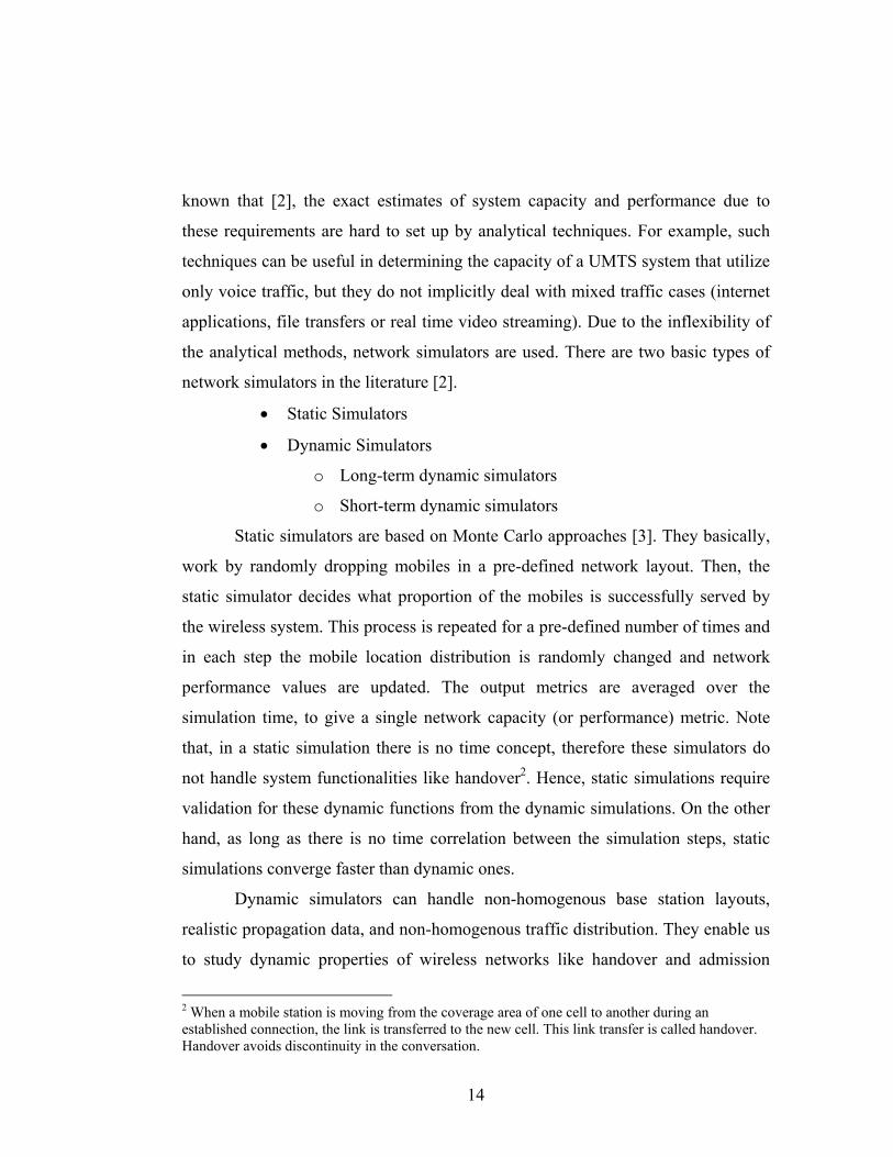
Static simulators are based on Monte Carlo approaches [3]. They basically,
work by randomly dropping mobiles in a pre-defined network layout. Then, the
static simulator decides what proportion of the mobiles is successfully served by
the wireless system. This process is repeated for a pre-defined number of times and
in each step the mobile location distribution is randomly changed and network
performance values are updated. The output metrics are averaged over the
simulation time, to give a single network capacity (or performance) metric. Note
that, in a static simulation there is no time concept, therefore these simulators do
not handle system functionalities like handover2. Hence, static simulations require
validation for these dynamic functions from the dynamic simulations. On the other
hand, as long as there is no time correlation between the simulation steps, static
simulations converge faster than dynamic ones.
Dynamic simulators can handle non-homogenous base station layouts,
realistic propagation data, and non-homogenous traffic distribution. They enable us
to study dynamic properties of wireless networks like handover and admission
2 When a mobile station is moving from the coverage area of one cell to another during an established connection, the link is transferred to the new cell. This link transfer is called handover. Handover avoids discontinuity in the conversation.
15
control3. Fundamentally, there are two different types of dynamic simulators in the
literature [2, 4], long-term and short-term. They are differentiated by their time-
scales of simulation, but indeed, they both include functions like admission control,
handover control and call dropping4. If our interest is focused on system capacity
or performance due to those dynamic functions, long-term simulations will satisfy
our needs. On the other hand, controls like time-slot selection, packet scheduling or
fast cell selection are handled in short-term dynamic simulators, because these
simulators are working in micro-timescales.
The major disadvantage of short-term simulations is their complexity and
long running times, because these simulators will be accessing the system with in
very short time scales. One of the best-known dynamic network simulators in the
literature is NS (Network Simulator) [5]. NS is a powerful network simulator that
has the ability of simulating vast number of different network schemes. It is a
discrete event simulator, which focuses on packet scheduling issues. There is no
specific module related to GSM and UMTS wireless systems in NS. It is possible
to extend NS (NS is an open source software) to simulate GSM and UMTS but NS
characteristics are not appropriate for these system level simulations. In estimating
the capacity of GSM like systems, long-term simulations satisfy all of the needs,
because it is much computationally easier. It is possible to use realistic propagation
data, environmental settings, traffic parameters and mobility generation in such a
fast simulator scheme.
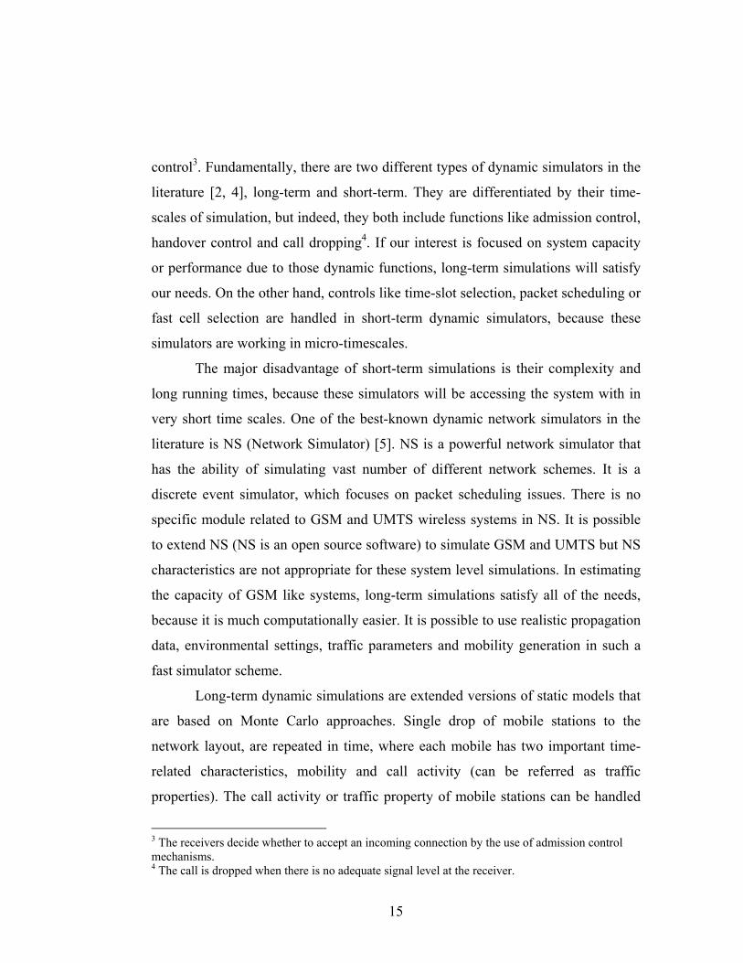
Long-term dynamic simulations are extended versions of static models that
are based on Monte Carlo approaches. Single drop of mobile stations to the
network layout, are repeated in time, where each mobile has two important time-
related characteristics, mobility and call activity (can be referred as traffic
properties). The call activity or traffic property of mobile stations can be handled
3 The receivers decide whether to accept an incoming connection by the use of admission control mechanisms. 4 The call is dropped when there is no adequate signal level at the receiver.
16
by turning on and off the mobiles during the simulation time. The times when the
mobile will turn on/off, is decided by an exponential traffic distribution. A long-
term simulator operates in relatively large time steps, in the order of seconds (1s –
10s).
In this thesis, long-term dynamic approach is used to simulate the two
wireless networks, GSM and UMTS. Instead of using the term “long-term dynamic
simulator”, “mobility simulator” is used, because mobility generation is explicitly
modeled in order to create a realistic dynamic simulator. The mobility model will
need to be designed carefully, if the intended traffic distribution is non-
homogenous, since the probability of a mobile passing through any point in the
service area is not uniform.
In order to generate realistic mobility patterns for the mobiles in the
simulation, a fast mobility generation algorithm is developed. In order to generate
random paths for mobile users, path-finding problem must be solved. This problem
can be solved by several routines; one of them is a graph-based solution. This
approach is accurate in finding shortest paths within a graph, but the algorithm is
slow and has running time of O(n2)[6]. The second approach to this problem is
step-taking algorithms, which are much faster then graph-based algorithms. In this
thesis, a step-taking algorithm is developed to solve the path-finding problem,
which has a running time of O(n).
1.3 Thesis Overview
In Chapter 2, first a brief description of mobility simulator that is developed
within this thesis study is given. Then, the input data needed for this simulator tool
is described. This data’s properties are explained and the effects of the changes in
this data on the simulator depicted network capacity (or performance) are
described. Chapter 2 also demonstrates how the mobility generation is achieved, by
17
giving different ways of solving the path-finding problem. The algorithm that is
implemented in dynamic simulator tool is depicted and the advantages and
disadvantages of this scheme are explained.
Chapter 3 presents GSM simulation tool developed within this thesis by
first giving a brief description of the working principles of GSM networks. Then,
GSM network planning is described and the effects of this planning phase on the
GSM service performance are represented. The simulation algorithm developed for
the GSM simulator tool is depicted and available results obtained from the
simulator is represented. Chapter 3 also provides a sample simulation of a pre-
designed GSM network layout. The output metrics are discussed and the effects of
the GSM system parameters on these metrics are illustrated.
Chapter 4 provides extensive coverage of UMTS. The medium access layer
of UMTS is different from the traditional access techniques like TDMA and
FDMA used in second-generation mobile systems, so this chapter introduces
CDMA technique. The configuration parameters of UMTS are illustrated and the
effects of these parameters on the performance metrics of UMTS are explained.
ITU performance tables are very important in modeling the 3G networks. These
tables are used to extract bit error rate requirements for different service demands,
so as the transmit powers of both the base and the mobile station. A sample
simulation’s results are depicted and discussed in this chapter.
Chapter 5 describes the deficiencies and advantages of using a dynamic
mobility simulator for predicting capacity and performance of wireless networks. It
also demonstrates the future work that can be done in order to improve the mobility
simulator.
18
Chapter 2 MOBILITY SIMULATION
The principal characteristic of mobile networks, which distinguishes them
from conventional fixed networks, is that the identity of the calling and called
subscriber is not associated with a fixed geographical location. The mobile
subscribers establish a wireless connection with the nearest available base station5.
In addition to this, they can make and receive call while they are moving. GSM and
UMTS support these functions.
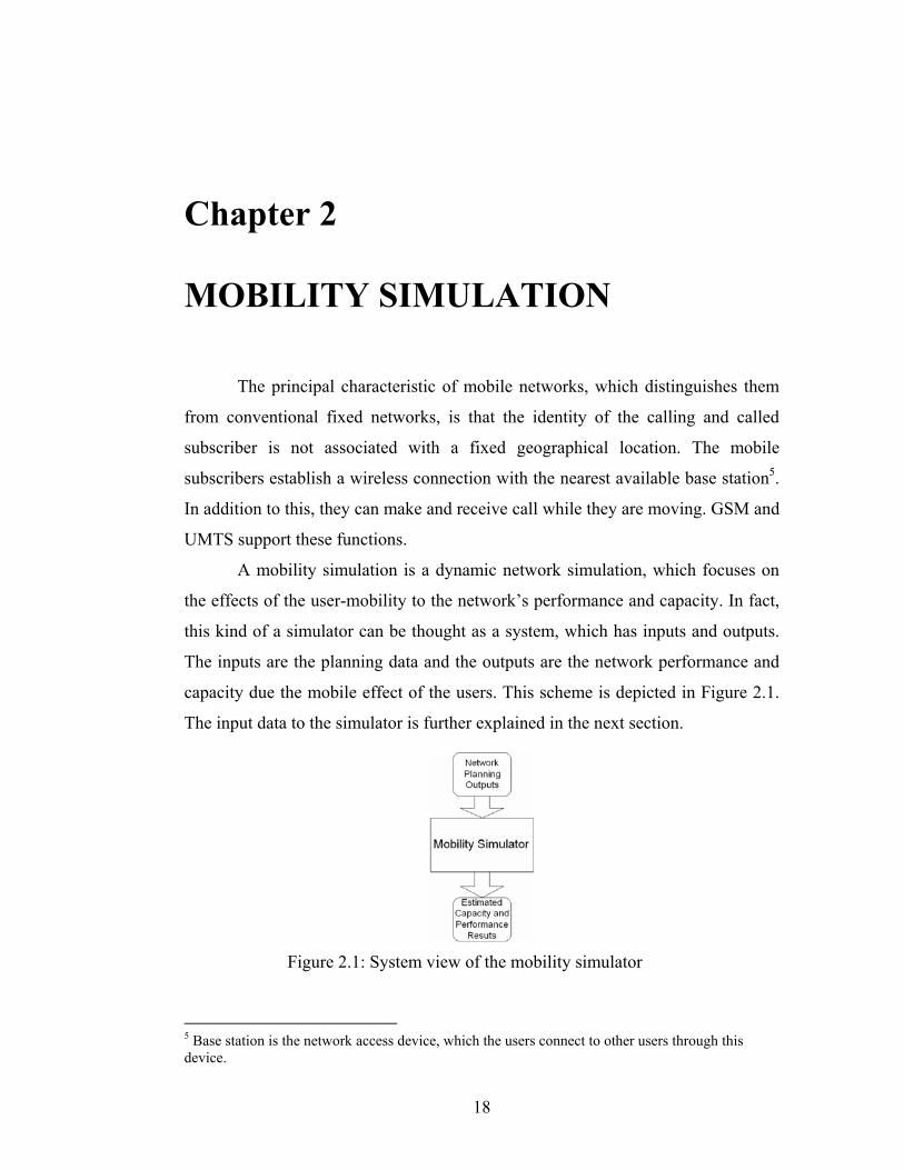
A mobility simulation is a dynamic network simulation, which focuses on
the effects of the user-mobility to the network’s performance and capacity. In fact,
this kind of a simulator can be thought as a system, which has inputs and outputs.
The inputs are the planning data and the outputs are the network performance and
capacity due the mobile effect of the users. This scheme is depicted in Figure 2.1.
The input data to the simulator is further explained in the next section.
Figure 2.1: System view of the mobility simulator
5 Base station is the network access device, which the users connect to other users through this device.
19
These simulations work on planned network layouts. They replicate the real world
usage of the wireless service. Actually, the simulator creates a virtual landscape, a
network infrastructure and mobile users that demand service from the wireless
network. A planning phase must occur to create the network layout, before starting
the simulation. This phase will generate the data needed for the mobility simulator.
The details of the outputs of the mobility simulator are explained in Chapters 3 and
4.
Mobility of these wireless users must be well modeled in order to make an
accurate simulation of a wireless network. The model will need to handle non-
homogenous traffic distribution, because the possibility of a user passing through
any particular tile of the service area is non-uniform.
The mobile users are categorized into two, pedestrians and vehicles. They
have an average speed of movement. These values are depicted in Table 2.1.
Mobile Users Speed (km/h) Pedestrians 3-5km/h
Vehicles 30-120km/h
Table 2.1: Mobile user speeds
As seen in the table above, the pedestrians have an average speed of 3-5km/h. In
the simulation, some portion of the pedestrians is assigned 3km/h speed and the
other portion is assigned 5km/h speed. This scheme is repeated for the vehicles in
the simulation.
After the speeds are assigned to the users, the movement paths must be
generated. At this stage, the direction of movement must be modeled. At the
beginning of the simulation, the mobile units are randomly dispersed over the
simulation area. Then, they choose a random destination point in the simulation
grid and start to move to reach to the destination. At the destination, they choose
another destination point. This procedure goes on until the simulation ends. While
reaching the destination, the mobile units must choose an appropriate direction of
20
movement. Path-finding algorithms solve the problem of choosing an appropriate
way to get to the destination. These algorithms and our way of solving the problem
are explained in section 2.2.
2.1 Data Needed for a Mobility Simulation
Mobility simulator simulates a planned network layout. Network layout
consists of the following items:
• Population in the service area
• Building data
• Places of the base stations
• Channel assignments to the base stations
• Propagation simulation results (Coverage data)
• Traffic profiles of the mobile users
The number of mobile users that are in the simulation is decided by using
the population information in the service area.
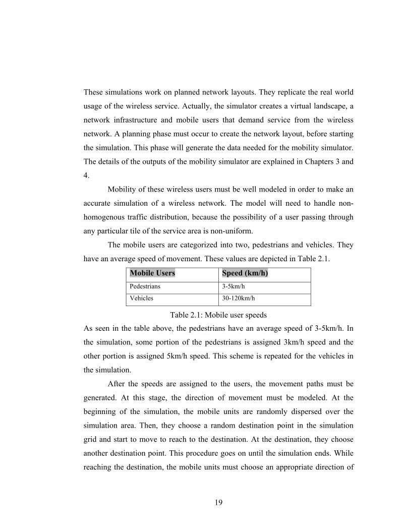
The simulated environment has buildings in it so the buildings must be
modeled in a way that the simulator can access. Simulator accesses the building
data for generating mobility patterns for the users simulated in the network, which
is explained in Section 2.2. An example of a building model is shown in Figure 2.2.
Figure 2.2: Building model
21
The blue painted parts in the above building model indicates buildings and the
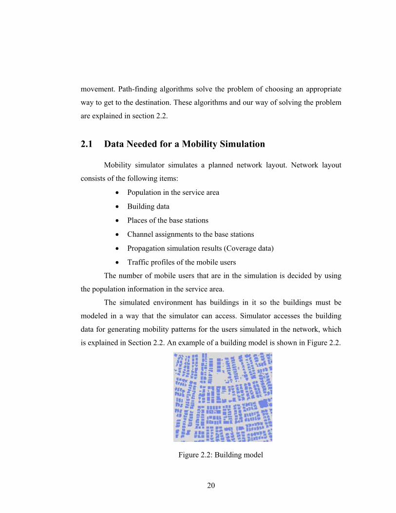
other areas are the streets passing through them. The model is then digitized with a
specific metric resolution. For example, if 5m is chosen as the resolution, the
building map is converted to a grid, where each grid element is 5m to 5m square.
This grid is stored in a text file, in order to be used by the mobility simulator
program. If a grid point coincides with a building, its value is set to –500. If it
coincides with a street area, its value is set to 0. The text file, which stores the
building model given in the above example, is depicted in Figure 2.3.
Figure 2.3: Building text file
The mobility generator reads this text file and stores in a two dimensional array.
The index of the array starts from (0,0), which indicates the first value in the text
file. This indexing is also depicted in Figure 2.3. The distance between two
consecutive grid points is defined by the metric resolution (5m in this example).
Places of the base stations and the channel assignment to those base stations
are discovered from traffic analyses. Traffic analysis uses the population
information in the service region in order to calculate the number of channels to
accommodate this offered traffic. Then the places of the base stations are
discovered by traffic analyses. Traffic analysis is not in the scope of this thesis,
because the mobility generator uses the outputs of this phase as inputs. This data is
also stored in a text file.
Propagation simulation results reveal the received signal power coming
from the base stations, all over the terrain. If the transmit power of the base stations
is known, a propagation algorithm is used to investigate the propagation of the
signal from the transmitter to the receiver. The mobility simulator needs
propagation simulation results, because the received signal power determines
Index:0,0
Index:2,2
22
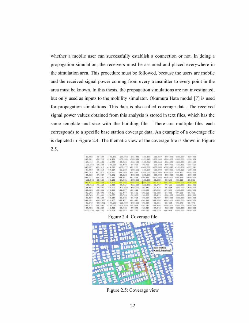
whether a mobile user can successfully establish a connection or not. In doing a
propagation simulation, the receivers must be assumed and placed everywhere in
the simulation area. This procedure must be followed, because the users are mobile
and the received signal power coming from every transmitter to every point in the
area must be known. In this thesis, the propagation simulations are not investigated,
but only used as inputs to the mobility simulator. Okumura Hata model [7] is used
for propagation simulations. This data is also called coverage data. The received
signal power values obtained from this analysis is stored in text files, which has the
same template and size with the building file. There are multiple files each
corresponds to a specific base station coverage data. An example of a coverage file
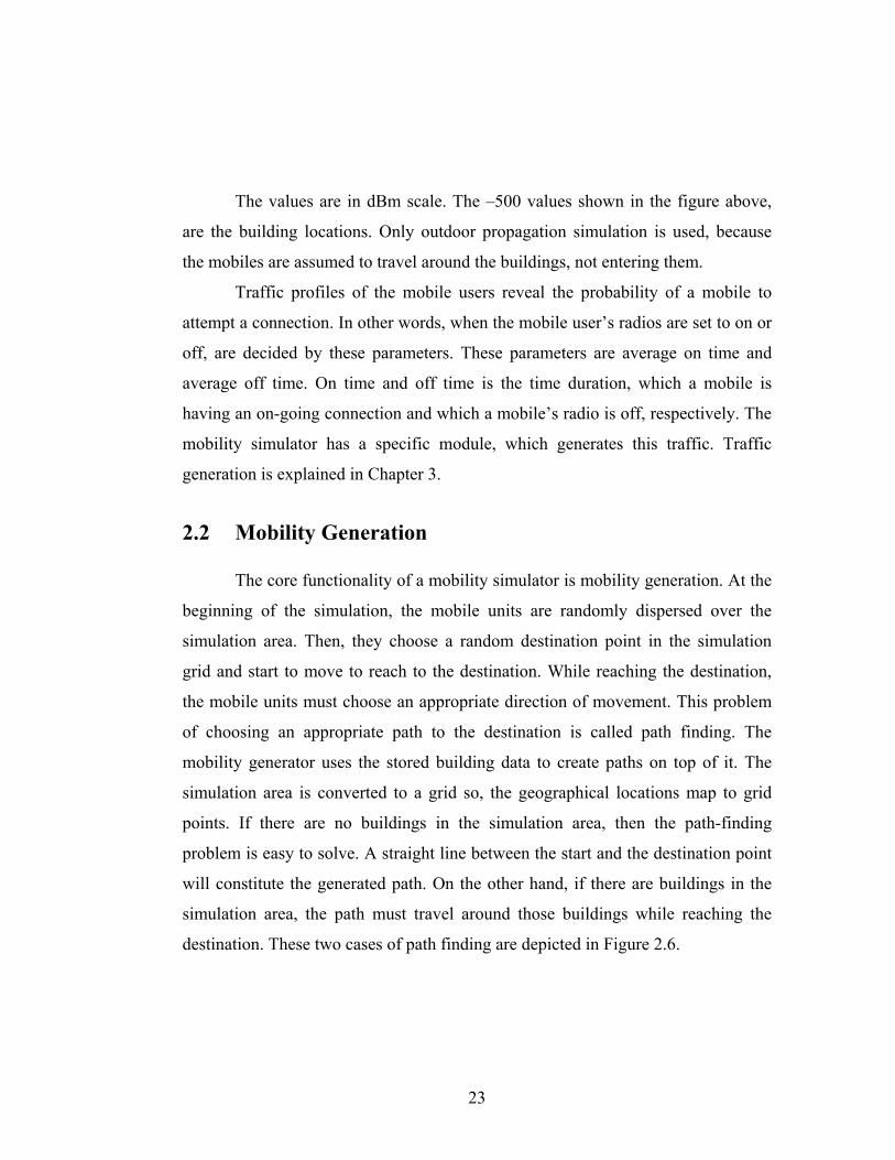
is depicted in Figure 2.4. The thematic view of the coverage file is shown in Figure
2.5.
Figure 2.4: Coverage file
Figure 2.5: Coverage view
23
The values are in dBm scale. The –500 values shown in the figure above,
are the building locations. Only outdoor propagation simulation is used, because
the mobiles are assumed to travel around the buildings, not entering them.
Traffic profiles of the mobile users reveal the probability of a mobile to
attempt a connection. In other words, when the mobile user’s radios are set to on or
off, are decided by these parameters. These parameters are average on time and
average off time. On time and off time is the time duration, which a mobile is
having an on-going connection and which a mobile’s radio is off, respectively. The
mobility simulator has a specific module, which generates this traffic. Traffic
generation is explained in Chapter 3.
2.2 Mobility Generation
The core functionality of a mobility simulator is mobility generation. At the
beginning of the simulation, the mobile units are randomly dispersed over the
simulation area. Then, they choose a random destination point in the simulation
grid and start to move to reach to the destination. While reaching the destination,
the mobile units must choose an appropriate direction of movement. This problem
of choosing an appropriate path to the destination is called path finding. The
mobility generator uses the stored building data to create paths on top of it. The
simulation area is converted to a grid so, the geographical locations map to grid
points. If there are no buildings in the simulation area, then the path-finding
problem is easy to solve. A straight line between the start and the destination point
will constitute the generated path. On the other hand, if there are buildings in the
simulation area, the path must travel around those buildings while reaching the
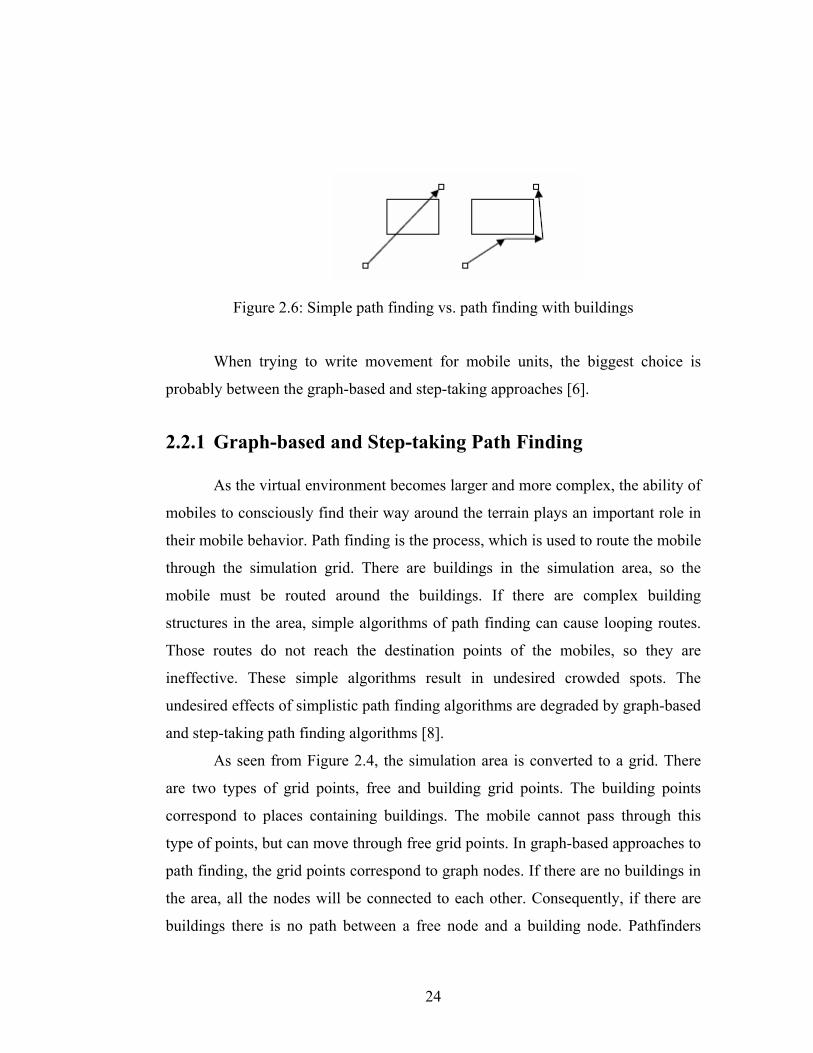
destination. These two cases of path finding are depicted in Figure 2.6.
24
Figure 2.6: Simple path finding vs. path finding with buildings
When trying to write movement for mobile units, the biggest choice is
probably between the graph-based and step-taking approaches [6].
2.2.1 Graph-based and Step-taking Path Finding
As the virtual environment becomes larger and more complex, the ability of
mobiles to consciously find their way around the terrain plays an important role in
their mobile behavior. Path finding is the process, which is used to route the mobile
through the simulation grid. There are buildings in the simulation area, so the
mobile must be routed around the buildings. If there are complex building
structures in the area, simple algorithms of path finding can cause looping routes.
Those routes do not reach the destination points of the mobiles, so they are
ineffective. These simple algorithms result in undesired crowded spots. The
undesired effects of simplistic path finding algorithms are degraded by graph-based
and step-taking path finding algorithms [8].
As seen from Figure 2.4, the simulation area is converted to a grid. There
are two types of grid points, free and building grid points. The building points
correspond to places containing buildings. The mobile cannot pass through this
type of points, but can move through free grid points. In graph-based approaches to
path finding, the grid points correspond to graph nodes. If there are no buildings in
the area, all the nodes will be connected to each other. Consequently, if there are
buildings there is no path between a free node and a building node. Pathfinders
25
look at the whole map and find a path for the unit to take. After that, the unit takes
each step prescribed by the pathfinder. Some graph bases path finding algorithms
are A* and Dijkstra [6]. These algorithms are complex and needs lots of pre-
processing. Also, graph based approaches are computationally complex and has a
running time of O[n2] where n is the number of nodes in the graph. The whole grid
must be first converted to a connected graph and then the algorithm must
investigate this entire graph to find a possible path between two nodes. These
algorithms are used to find the shortest path and some of them are very accurate [6,
8].
In this mobility simulator, there is no need for a shortest path for the mobile
units, because their movement is modeled as random motion. The only criterion for
the path-finding problem in the mobility simulation is that the algorithm must find
a path between any two points in the simulation grid.
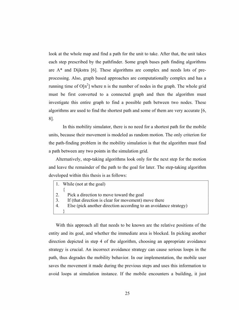
Alternatively, step-taking algorithms look only for the next step for the motion
and leave the remainder of the path to the goal for later. The step-taking algorithm
developed within this thesis is as follows:
1. While (not at the goal) { 2. Pick a direction to move toward the goal 3. If (that direction is clear for movement) move there 4. Else (pick another direction according to an avoidance strategy) }
With this approach all that needs to be known are the relative positions of the
entity and its goal, and whether the immediate area is blocked. In picking another
direction depicted in step 4 of the algorithm, choosing an appropriate avoidance
strategy is crucial. An incorrect avoidance strategy can cause serious loops in the
path, thus degrades the mobility behavior. In our implementation, the mobile user
saves the movement it made during the previous steps and uses this information to
avoid loops at simulation instance. If the mobile encounters a building, it just
26
moves around it staying besides the building. This behavior is supplied by the
history information of the path of that mobile.
First, all the mobile units are randomly dispersed over the simulation area
(uniformly). Then, for every mobile unit, a random destination point is chosen. The
algorithms duty is to move the mobile unit (with the specified speed) in a path such
that the destination point is reached. When a mobile user reaches its specific
destination point, another random destination is chosen, and this process continues
within the specified simulation duration. Choosing destination points for every user
in the simulation, supplies the ability of making more and less crowded areas in the
simulation area. A random variable chooses the coordinates of the destination
points. By adjusting the probability of the random variable to choose more or less
in a specific region, some places can be more crowded (visited by the mobiles
more), on the average. The C# code of the algorithm is depicted in the appendix.
27
Chapter 3 GSM SIMULATION GSM simulator models the system with realistic mobile user traffic
distribution, an accurate propagation data on top of a real building data and
generated user mobility. The propagation simulation is done with the usage of a
real building and terrain data before the actual GSM mobility simulation is
established. Then, the received power values are written to a simple file and read
by the GSM mobility simulator in order to determine whether a mobile user can
connect to the system or not. The RLC (Radio Link Control) layer in the GSM
structure is modeled in the simulator that simply determines whether the user can
access to the system. The simulator is written in C# in .Net environment.
With the intention of analyzing the performance of a GSM cellular network
design, GSM mobility simulator is developed. Simulation models the GSM system
and the cellular environment with precise models of signal propagation, user
mobility and traffic distribution. This application works as fallows. First, a
simulation model of the network is created, and then a user population is virtually
generated. With these virtual mobile users and traffic characteristics, the planned
network model is simulated. The users are mobile so, the mobility generator
produces their routes. In addition, the data rate demands of the users are controlled
by these simulation parameters. The simulation, at the end, generates graphs and
reports that inform GSM network performance related metrics.
The GSM mobility simulator described in this thesis can be applied to many
areas such as, design of physical network layout, assessing the impact of network
adjustments and configuration changes, analyzing the effect of new network
28
components such as base stations, handsets and demonstrating the outcome of
service profiles [25]. The simulator described in this thesis is a dynamic network
level simulator for the performance evaluation of GSM. Dynamic simulator models
the time correlation between the events, which is useful in determining the overall
performance of these types of wireless networks. In each simulation step, mobiles
move along their paths and this mobility behavior leads to handovers, which play
an important role in service quality and capacity of the GSM network [9].
3.1 GSM Overview
GSM denotes Global System for Mobile Communications. It is referred as a
second-generation wireless network. It serves voice only traffic with a data rate of
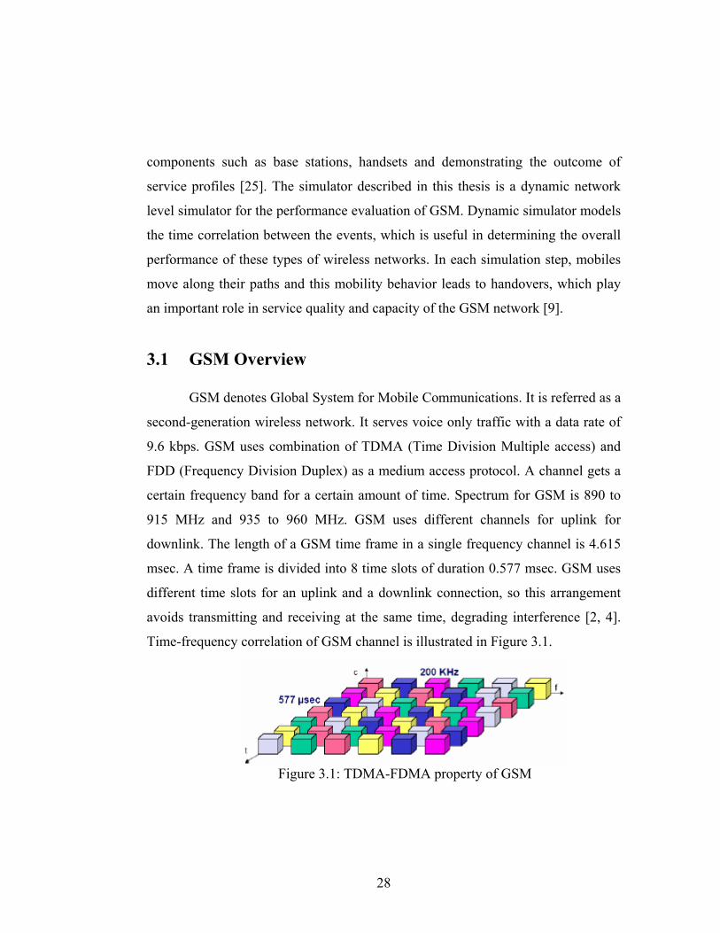
9.6 kbps. GSM uses combination of TDMA (Time Division Multiple access) and
FDD (Frequency Division Duplex) as a medium access protocol. A channel gets a
certain frequency band for a certain amount of time. Spectrum for GSM is 890 to
915 MHz and 935 to 960 MHz. GSM uses different channels for uplink for
downlink. The length of a GSM time frame in a single frequency channel is 4.615
msec. A time frame is divided into 8 time slots of duration 0.577 msec. GSM uses
different time slots for an uplink and a downlink connection, so this arrangement
avoids transmitting and receiving at the same time, degrading interference [2, 4].
Time-frequency correlation of GSM channel is illustrated in Figure 3.1.
Figure 3.1: TDMA-FDMA property of GSM
29
Spectrum is limited but demand is high, so in GSM, a cellular structure is
used. Every cell has a base station and assigned frequency set. Therefore, every
additional cell can accommodate more users. The same frequency channel can be
used in two or more cells, so this frequency reuse causes interference of signals. As
the interference level increases, the receivers are not able to demodulate the signal.
This interference limits large frequency reuse ratios in GSM.
3.2 GSM Network Planning
Network planning is the first step while establishing a wireless network.
Electromagnetic spectrum is a unique resource across a vast range from 3 kHz to
300 GHz. Unlike other physical resources, it cannot be depleted. However, as radio
signals overlay each other in an additive way, there exist interdependencies and
thus rivalry among users. In an extreme case, interference can damage the radio
signals of all participants to the point where they become unrecognizable and
therefore useless. Planning in these networks is crucial because good network
planning means minimum interference on the system. Planning the network
beforehand increases the service quality and capacity. The other necessity of
planning is economy of investment [10, 11]. The resources are expensive so they
must be optimally used.
Network planning data is the input to the mobility simulator. Therefore, a
planned network is needed in order to make a mobility simulation. The planning
data is obtained from two analyses:
• Traffic Planning
• Coverage Analysis
Traffic planning data is places of the base stations and the channel assignments to
those base stations. Coverage analysis reveals the received signal power values that
are coming from the base stations, all over the service area. In order to make a
30
coverage analysis the building data and terrain profile are used. At the beginning of
the simulation, these data are fed to the simulator.
3.3 Configuration Parameters and Performance Metrics
The configuration parameters can be classified into three main parts.
• Mobile user’s parameters
o Speed
o Traffic profile
• System configuration parameters
o Base station locations
o Number of voice channels assigned to each base station
o Received signal power over the simulation area, for each base
station (dBm)
o Handover Threshold (dBm)
o Minimum received signal power for communication (dBm)
o SINAD threshold (dB)
o Hysteris Value (dB)
• Simulation parameters
o Physical dimensions of the simulation area
o Duration of simulation
o Number of mobile users to be simulated
Speed of the mobiles is used when generating the movement of the users in
the simulation area. Traffic profile parameters are used in producing the random
traffic for the mobiles. There are two traffic related parameters, on time and off
time. On time is the time duration, when the mobile is established a link to a base
station. Off time is the period, when the mobile’s radio is off. These both time
31
intervals are modeled as negative exponential random distribution, which the
formula for the random number is given in (3.1).
(3.1)
where,
µ: Mean of the exponential random number
E: Exponential random number
U: Uniform random number between 0 and 1
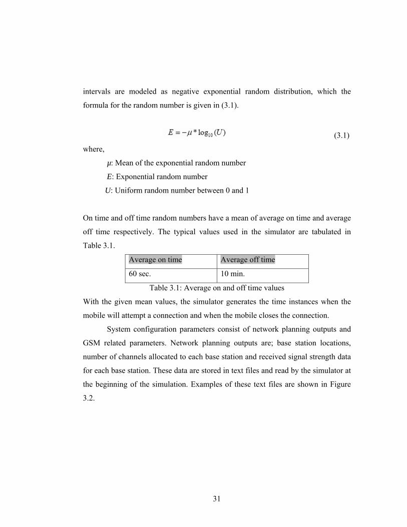
On time and off time random numbers have a mean of average on time and average
off time respectively. The typical values used in the simulator are tabulated in
Table 3.1.
Average on time Average off time
60 sec. 10 min.
Table 3.1: Average on and off time values
With the given mean values, the simulator generates the time instances when the
mobile will attempt a connection and when the mobile closes the connection.
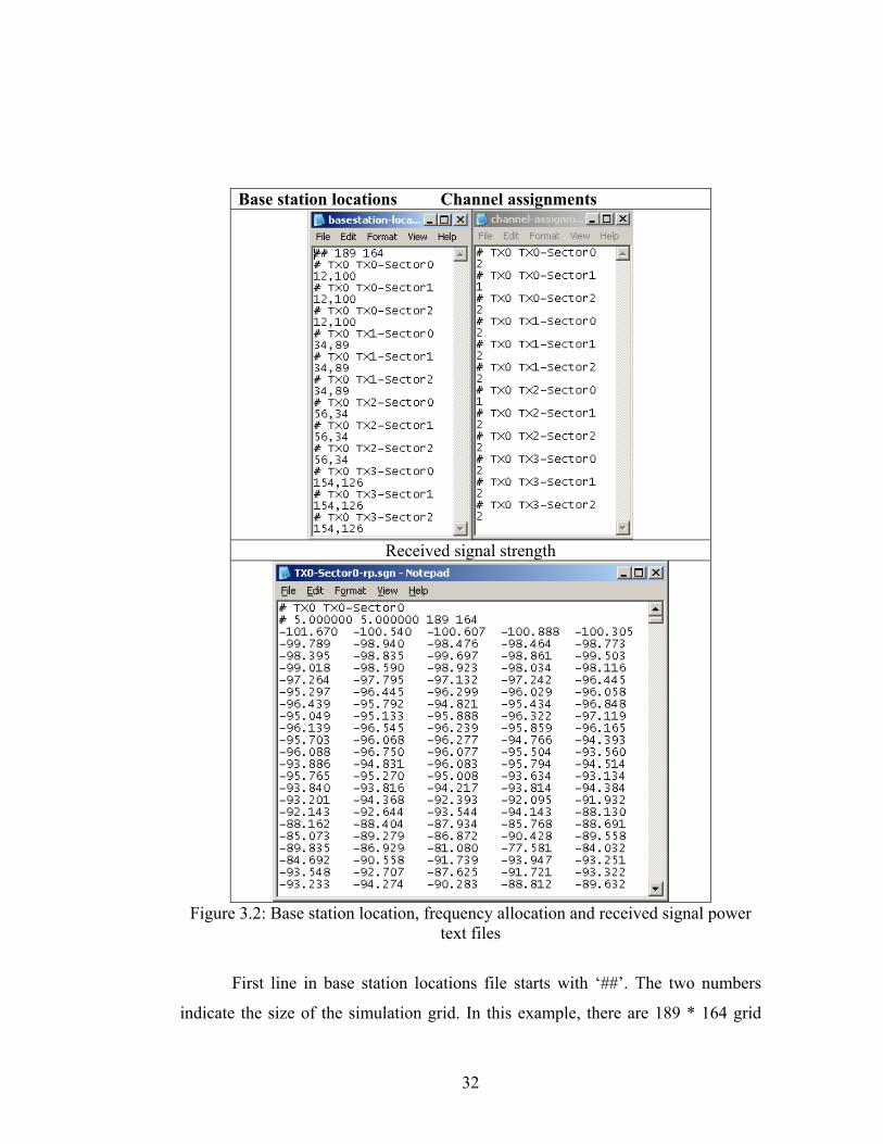
System configuration parameters consist of network planning outputs and
GSM related parameters. Network planning outputs are; base station locations,
number of channels allocated to each base station and received signal strength data
for each base station. These data are stored in text files and read by the simulator at
the beginning of the simulation. Examples of these text files are shown in Figure
3.2.
32
Base station locations Channel assignments
Received signal strength
Figure 3.2: Base station location, frequency allocation and received signal power
text files
First line in base station locations file starts with ‘##’. The two numbers
indicate the size of the simulation grid. In this example, there are 189 * 164 grid
33
points in the simulation area. The metric resolution is 5 m. so; the physical
dimension of the region is 189*5=945m to 164*5=820m. The lines starting with ‘#’
indicates the id’s of the base stations and the followings lines denotes the location
that base station in the grid. For example, the ‘TX-0 Sector 0’ base station is
located at (12,100) in the grid. Note that, there are three sectors for each cell,
because 120o sectored base stations are used. Three sectors of a site6 are located at
the same spot in the grid.
Channel assignment file consists of the number of channels allocated to
each base station. The lines starting with ‘#’ denotes the id’s of the base stations
and the following lines denotes the number of frequency channel allocated to that
base station. For example, the site with id ‘TX-1 Sector2’ has 2 frequency
channels. Every frequency channel has 8 time slots, 1 reserved for control issues.
Therefore, there exists 2*8 – 1 = 15 traffic channels in that base station. This
means, 15 mobiles can connect to that base station at the same time. TDMA
synchronizes the time slots, so there is no interference between mobiles that are
using the same frequency band in a single cell. On the other hand, in GSM the
same frequency band can be assigned to two or more different base stations. This
causes interference and limits the usage of large frequency reuse ratios7.
Received signal strength files consist of the powers of the signal transmitted
(in dBm) from each base station all over the terrain. The first line that is starting
with ‘#’ denotes the base station id. The second line has the metric resolution and
the corresponding grid size of the simulation area. For example, Figure 3.2 shows a
signal power file for base station ‘TX-0 Sector0’. The file has a metric resolution of
5m to 5m and has a grid size of 189 to 164. If a mobile is located at 0,0 location in
6 Site corresponds to a cell in GSM 7 Frequency reuse: The ability of specific channels assigned to a single cell to be used again in another cell, when there is enough distance between the two cells to prevent co-channel interference from affecting service quality. The technique enables a cellular system to increase capacity with a limited number of channels.
34
the simulation grid and connected to base station ‘TX-0 Sector0’, the received
signal strength coming from the base station is –101.67 dBm.
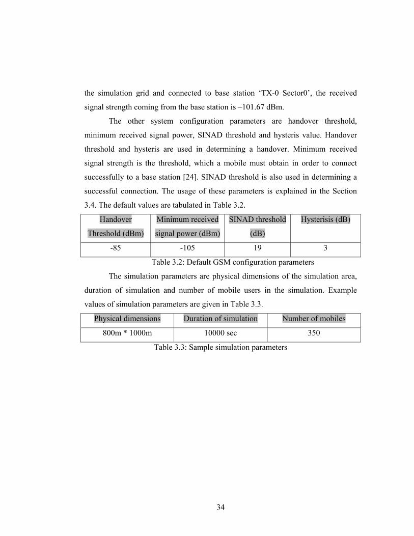
The other system configuration parameters are handover threshold,
minimum received signal power, SINAD threshold and hysteris value. Handover
threshold and hysteris are used in determining a handover. Minimum received
signal strength is the threshold, which a mobile must obtain in order to connect
successfully to a base station [24]. SINAD threshold is also used in determining a
successful connection. The usage of these parameters is explained in the Section
3.4. The default values are tabulated in Table 3.2.
Handover
Threshold (dBm)
Minimum received
signal power (dBm)
SINAD threshold
(dB)
Hysterisis (dB)
-85 -105 19 3
Table 3.2: Default GSM configuration parameters
The simulation parameters are physical dimensions of the simulation area,
duration of simulation and number of mobile users in the simulation. Example
values of simulation parameters are given in Table 3.3.
Physical dimensions Duration of simulation Number of mobiles
800m * 1000m 10000 sec 350
Table 3.3: Sample simulation parameters
35
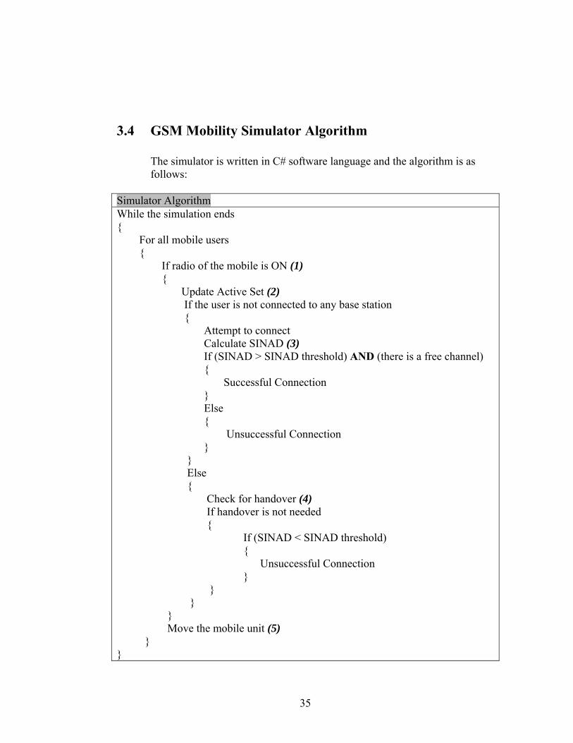
3.4 GSM Mobility Simulator Algorithm
The simulator is written in C# software language and the algorithm is as follows:
Simulator Algorithm While the simulation ends { For all mobile users { If radio of the mobile is ON (1) { Update Active Set (2) If the user is not connected to any base station { Attempt to connect Calculate SINAD (3) If (SINAD > SINAD threshold) AND (there is a free channel) { Successful Connection } Else { Unsuccessful Connection } } Else { Check for handover (4) If handover is not needed { If (SINAD < SINAD threshold) { Unsuccessful Connection } } } } Move the mobile unit (5) } }
36
Statement (1) is decided by the exponential on/off traffic generation procedure.
Active set stated in (2) is defined as eight base stations with maximum received
power at the recent position of the mobile user. When the mobile’s radio is on, the
mobile will attempt to connect to the first base station in the active set (which have
the highest received signal power). SINAD stated in (3) is the signal to interference
+ noise ratio. SINAD formulation is depicted in (3.2).
SSINADI N
=+
(3.2)
where,
S: Signal power received from the serving base station
I: Total interfering signal power received from the other base station
N: Thermal Noise (N=k*T*B)
k: Boltzman’s constant
T: Effective temperature
B: Channel bandwidth
(SINAD is due to frequency reuse and thermal noise in the GSM network)
The calculated SINAD value is compared with the SINAD threshold depicted in
the system parameters. If the calculated value is lower than the threshold,
connection cannot be established with that base station. Handover decision is taken
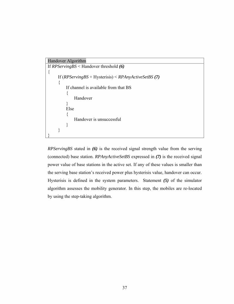
by the handover algorithm, which is depicted in statement (4). The algorithm is as
follows:
37
Handover Algorithm If RPServingBS < Handover threshold (6) { If (RPServingBS + Hysterisis) < RPAnyActiveSetBS (7) { If channel is available from that BS { Handover } Else { Handover is unsuccessful } } }
RPServingBS stated in (6) is the received signal strength value from the serving
(connected) base station. RPAnyActiveSetBS expressed in (7) is the received signal
power value of base stations in the active set. If any of these values is smaller than
the serving base station’s received power plus hysterisis value, handover can occur.
Hysterisis is defined in the system parameters. Statement (5) of the simulator
algorithm assesses the mobility generator. In this step, the mobiles are re-located
by using the step-taking algorithm.
38
3.5 Results Obtained from the Simulator
After the simulation ends successfully, the results are taken and visualized
to the end-user. The outputs of the simulator show the simulation history and the
GSM network performance. Obtained results are tabulated in Table 3.4.
3.5.1 Coverage Analysis 3.5.2 Localization 3.5.3 Successful / Unsuccessful Connections 3.5.4 Successful / Unsuccessful Handovers 3.5.5 Channel Utilization 3.5.6 Test Mobile Signal Profile
Table 3.4: Results obtained from the GSM mobility simulator In each sub-chapter tabulated in Table 3.4, the methodology of obtaining the
corresponding results is explained and sample snapshots of the results are given.
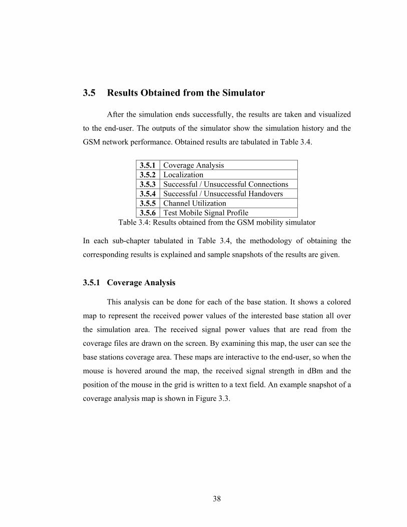
3.5.1 Coverage Analysis
This analysis can be done for each of the base station. It shows a colored
map to represent the received power values of the interested base station all over
the simulation area. The received signal power values that are read from the
coverage files are drawn on the screen. By examining this map, the user can see the
base stations coverage area. These maps are interactive to the end-user, so when the
mouse is hovered around the map, the received signal strength in dBm and the
position of the mouse in the grid is written to a text field. An example snapshot of a
coverage analysis map is shown in Figure 3.3.
39
Figure 3.3: Coverage map snapshot
The red parts in this graph show the high coverage regions. These regions consist
of points, which have higher received power values than the blue parts of the
graph.
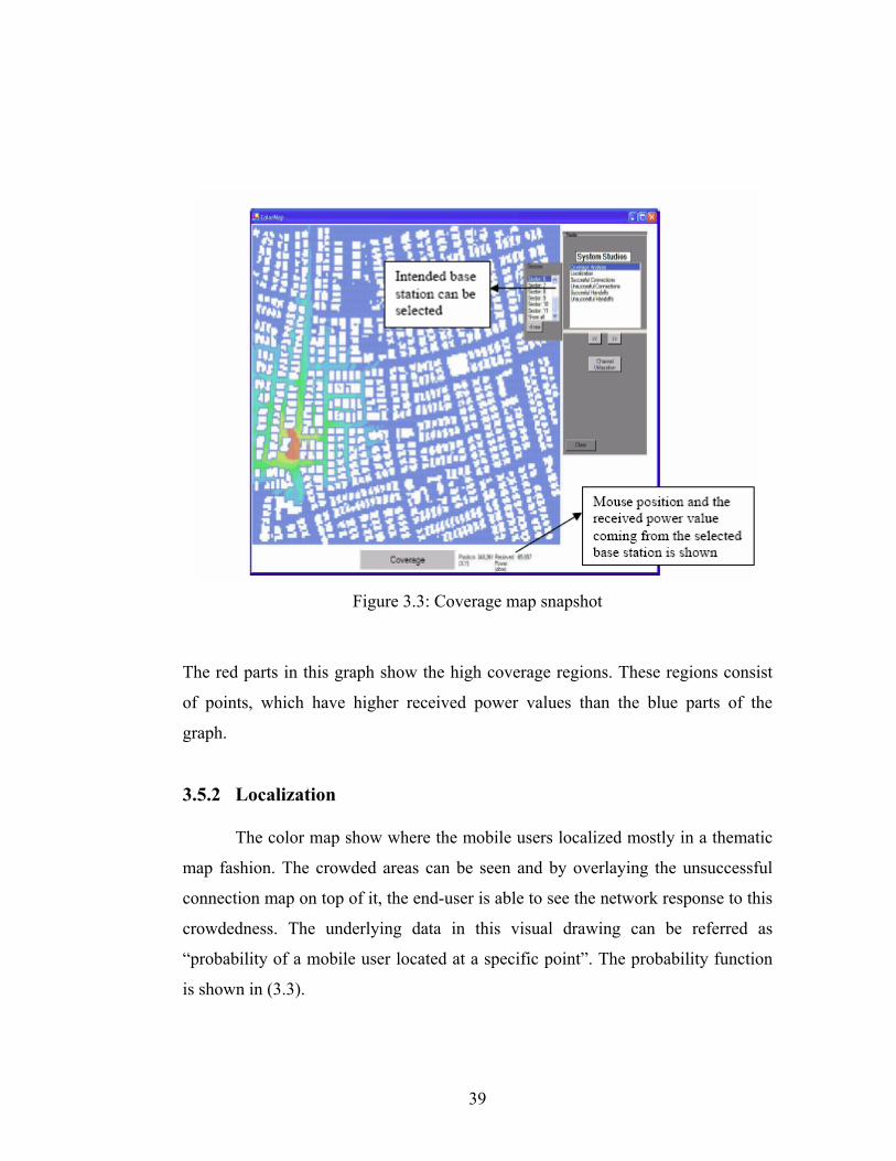
3.5.2 Localization
The color map show where the mobile users localized mostly in a thematic
map fashion. The crowded areas can be seen and by overlaying the unsuccessful
connection map on top of it, the end-user is able to see the network response to this
crowdedness. The underlying data in this visual drawing can be referred as
“probability of a mobile user located at a specific point”. The probability function
is shown in (3.3).
40
(3.3)
where,
p(x,y): Probability that there is a user located at point x, y in the simulation
environment. Tstep(x,y,t): Total number of users located at point x, y at time t, during the simulation. A probability of 1 is drawn with red. As the probability decreases to 0, the colors
change to blue. An example snapshot of localization map is shown in Figure 3.4.
The red parts indicate the crowded regions in the simulation. This is an example of
a city center simulation. As long as the center of the city is more crowded then the
other parts, by choosing more destination points in the center region, we can make
the center parts of the city more crowded.
Figure 3.4: Localization map snapshot
41
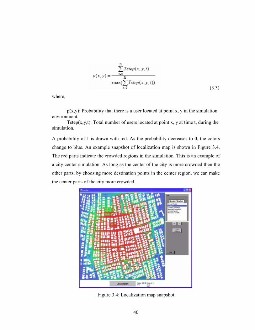
3.5.3 Successful/Unsuccessful Connections
The connection statuses, which are monitored by the simulator, are stored
and visualized to the end user. When a user attempts a call, the status of that call is
stored. If that user is able to connect to the network, this call becomes a successful
connection and shown in green spots on the simulation grid. On the other hand,
unsuccessful attempts are shown in red spots. The more crowded locations in the
simulation area, creates more unsuccessful connections because the number of
available channels on these regions decreases due to high traffic demand as shown
in Figure 3.5. In addition, less covered regions, which can be visualized by the
coverage analysis map, generates red spots. In these areas, the received signal
powers are low so active set becomes smaller and the user’s call attempts turns out
to be unsuccessful.
Figure 3.5: Successful/Unsuccessful Connections snapshot
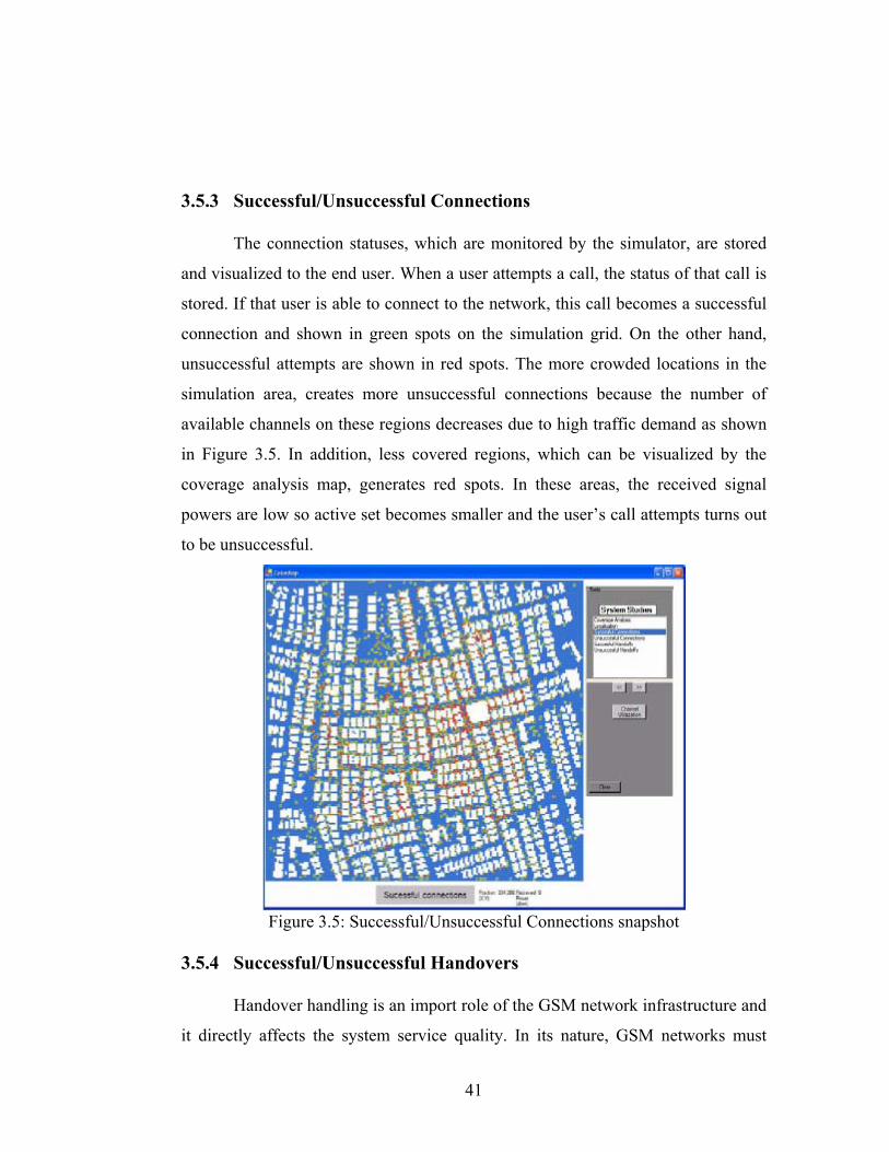
3.5.4 Successful/Unsuccessful Handovers
Handover handling is an import role of the GSM network infrastructure and
it directly affects the system service quality. In its nature, GSM networks must
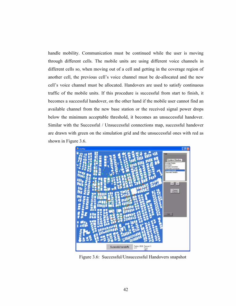
42
handle mobility. Communication must be continued while the user is moving
through different cells. The mobile units are using different voice channels in
different cells so, when moving out of a cell and getting in the coverage region of
another cell, the previous cell’s voice channel must be de-allocated and the new
cell’s voice channel must be allocated. Handovers are used to satisfy continuous
traffic of the mobile units. If this procedure is successful from start to finish, it
becomes a successful handover, on the other hand if the mobile user cannot find an
available channel from the new base station or the received signal power drops
below the minimum acceptable threshold, it becomes an unsuccessful handover.
Similar with the Successful / Unsuccessful connections map, successful handover
are drawn with green on the simulation grid and the unsuccessful ones with red as
shown in Figure 3.6.
Figure 3.6: Successful/Unsuccessful Handovers snapshot
43
Monitoring handovers are the main interest of dynamic simulators and they
must be well modeled. Handovers cause traffic overhead on the GSM network and
bad handling of handovers degrades system quality. If there are unsuccessful
handovers in the simulation, more channels must be assigned to the base station in
order to serve this offered traffic.
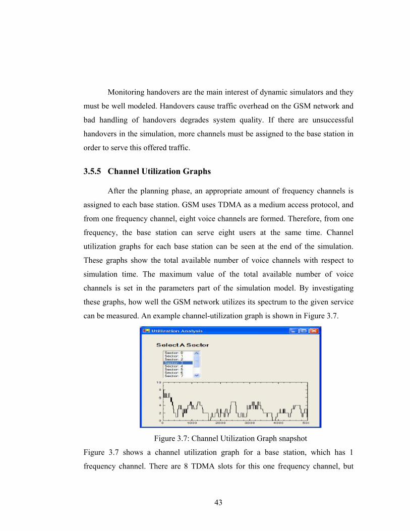
3.5.5 Channel Utilization Graphs
After the planning phase, an appropriate amount of frequency channels is
assigned to each base station. GSM uses TDMA as a medium access protocol, and
from one frequency channel, eight voice channels are formed. Therefore, from one
frequency, the base station can serve eight users at the same time. Channel
utilization graphs for each base station can be seen at the end of the simulation.
These graphs show the total available number of voice channels with respect to
simulation time. The maximum value of the total available number of voice
channels is set in the parameters part of the simulation model. By investigating
these graphs, how well the GSM network utilizes its spectrum to the given service
can be measured. An example channel-utilization graph is shown in Figure 3.7.
Figure 3.7: Channel Utilization Graph snapshot
Figure 3.7 shows a channel utilization graph for a base station, which has 1
frequency channel. There are 8 TDMA slots for this one frequency channel, but
44
one slot is reserved for control issues. The maximum available channel in this
graph is 7 (1*8-1).
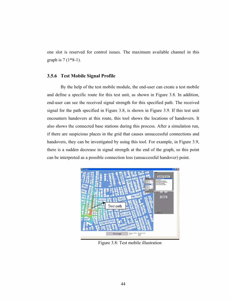
3.5.6 Test Mobile Signal Profile
By the help of the test mobile module, the end-user can create a test mobile
and define a specific route for this test unit, as shown in Figure 3.8. In addition,
end-user can see the received signal strength for this specified path. The received
signal for the path specified in Figure 3.8, is shown in Figure 3.9. If this test unit
encounters handovers at this route, this tool shows the locations of handovers. It
also shows the connected base stations during this process. After a simulation run,
if there are suspicious places in the grid that causes unsuccessful connections and
handovers, they can be investigated by using this tool. For example, in Figure 3.9,
there is a sudden decrease in signal strength at the end of the graph, so this point
can be interpreted as a possible connection loss (unsuccessful handover) point.
Figure 3.8: Test mobile illustration
45
Figure 3.9: Test mobile signal profile
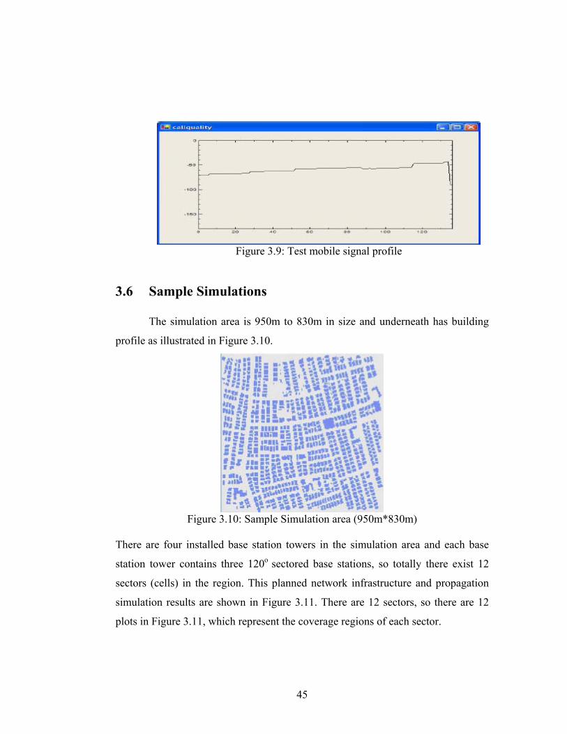
3.6 Sample Simulations
The simulation area is 950m to 830m in size and underneath has building
profile as illustrated in Figure 3.10.
Figure 3.10: Sample Simulation area (950m*830m)
There are four installed base station towers in the simulation area and each base
station tower contains three 120o sectored base stations, so totally there exist 12
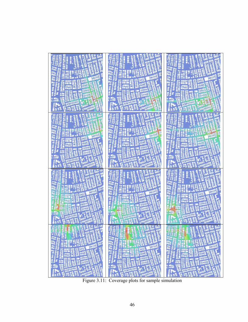
sectors (cells) in the region. This planned network infrastructure and propagation
simulation results are shown in Figure 3.11. There are 12 sectors, so there are 12
plots in Figure 3.11, which represent the coverage regions of each sector.
46
Figure 3.11: Coverage plots for sample simulation
47
In all of the sectors, 2 frequency channels are assigned as a result of traffic
planning phase. Therefore, totally there are 12 * 2 = 24 frequency channels in the
network. Each frequency channel has 8 time slots, 1 reserved for control issues, so
there exist 24 * (8-1) = 168 traffic channels in the whole GSM network.
Consequently, at a specific instance, maximum 168 mobile users can connect to
this GSM network. On the other hand, mobility brings capacity degradations to the
system, because, the user population changes dynamically resulting in crowded
locations (hot spots). By using this mobility simulation, these regions will be
determined. Using this scenario, two different simulations are done. First one is a
less crowded (relatively less crowded) city simulation containing 100 mobile users.
On the other hand, second simulation is a crowded city simulation containing 300
mobile users on the area.
Mobility behaviors are the same for the two simulations, the mobile users
travel at a speed of 5 km/h. In addition, traffic behaviors are similar; the mobiles
have average on time 60sec and average off time 600sec in both of the simulations.
These parameters are tabulated in Table 3.5.
Simulation1 Simulation2 Number of mobiles 100 300 Mobile Speed (km/h) 5 5 Average on time (sec) 60 60 Average off time (sec) 600 600 Total simulation time (sec) 10000 10000
Table 3.5: Sample simulation parameters 3.6.1 Results And Discussion
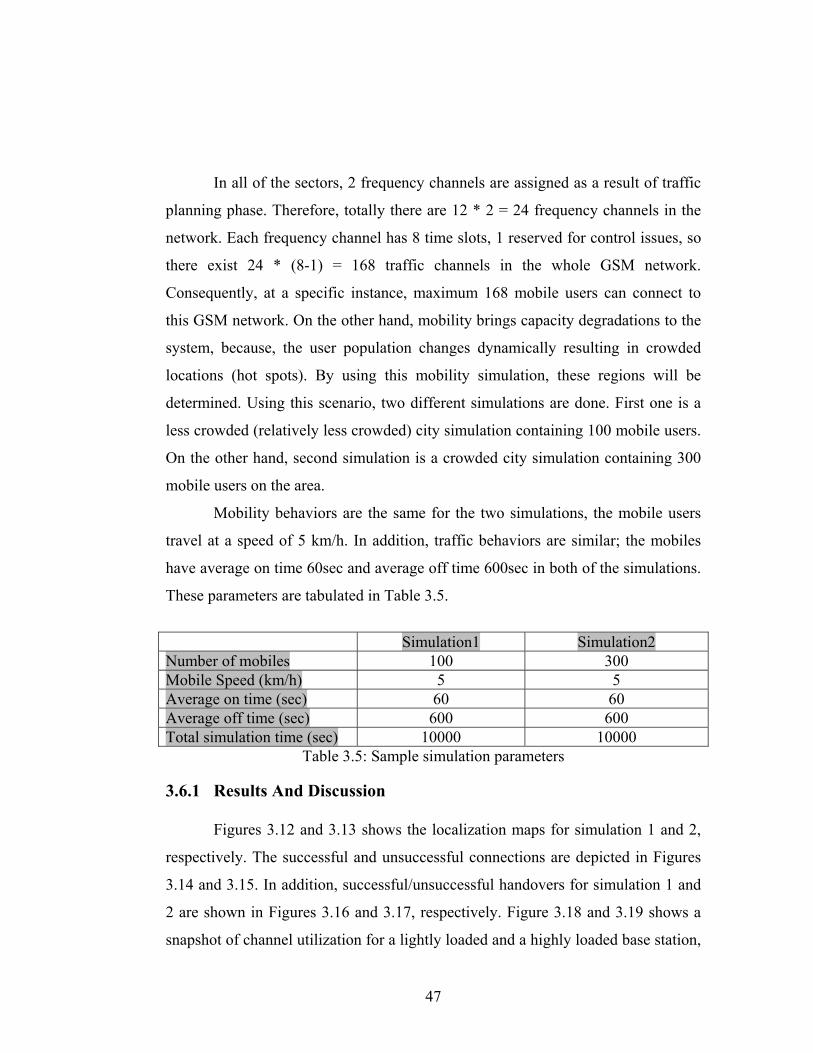
Figures 3.12 and 3.13 shows the localization maps for simulation 1 and 2,
respectively. The successful and unsuccessful connections are depicted in Figures
3.14 and 3.15. In addition, successful/unsuccessful handovers for simulation 1 and
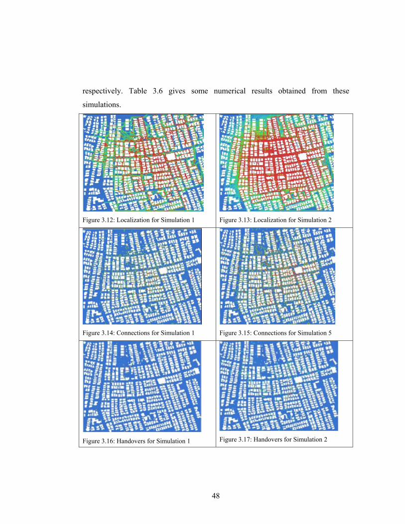
2 are shown in Figures 3.16 and 3.17, respectively. Figure 3.18 and 3.19 shows a
snapshot of channel utilization for a lightly loaded and a highly loaded base station,
48
respectively. Table 3.6 gives some numerical results obtained from these
simulations.
Figure 3.12: Localization for Simulation 1
Figure 3.13: Localization for Simulation 2
Figure 3.14: Connections for Simulation 1
Figure 3.15: Connections for Simulation 5
Figure 3.16: Handovers for Simulation 1
Figure 3.17: Handovers for Simulation 2
49
Figure 3.18: Lightly loaded base station’s channel utilization
Figure 3.19: Highly loaded base station’s channel utilization
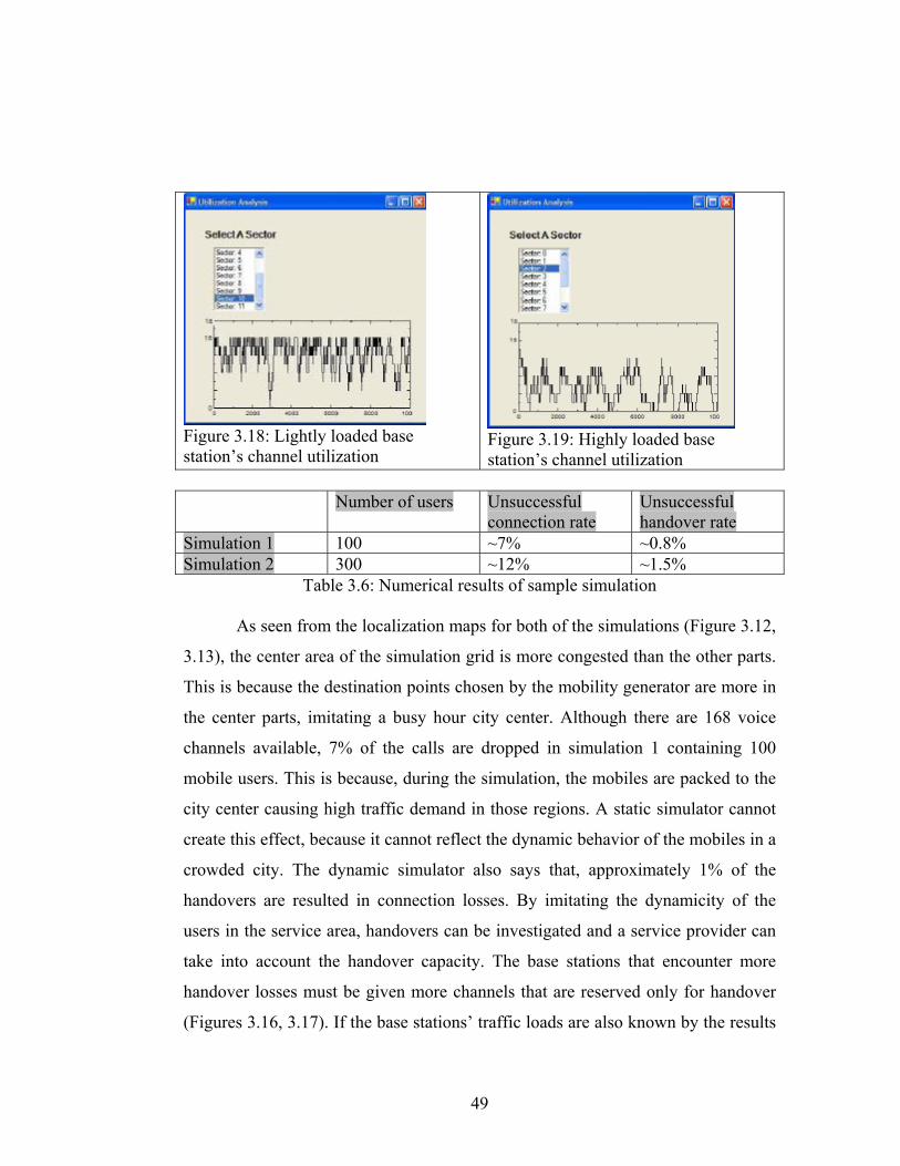
Number of users Unsuccessful
connection rate Unsuccessful handover rate
Simulation 1 100 ~7% ~0.8% Simulation 2 300 ~12% ~1.5%
Table 3.6: Numerical results of sample simulation
As seen from the localization maps for both of the simulations (Figure 3.12,
3.13), the center area of the simulation grid is more congested than the other parts.
This is because the destination points chosen by the mobility generator are more in
the center parts, imitating a busy hour city center. Although there are 168 voice
channels available, 7% of the calls are dropped in simulation 1 containing 100
mobile users. This is because, during the simulation, the mobiles are packed to the
city center causing high traffic demand in those regions. A static simulator cannot
create this effect, because it cannot reflect the dynamic behavior of the mobiles in a
crowded city. The dynamic simulator also says that, approximately 1% of the
handovers are resulted in connection losses. By imitating the dynamicity of the
users in the service area, handovers can be investigated and a service provider can
take into account the handover capacity. The base stations that encounter more
handover losses must be given more channels that are reserved only for handover
(Figures 3.16, 3.17). If the base stations’ traffic loads are also known by the results
50
(Figures 3.18, 3.19) of a dynamic simulation (using channel utilization graphs),
more frequency channels can be assigned to those that have high traffic load. As
expected, in simulation 2, there are more losses of connection than simulation 1,
because, the number of users in the second simulation is three folds compared to
the first simulation (Figures 3.14, 3.15 and Table 3.6). 90% of the unsuccessful
connections are in the central locations of the simulation area; this is because
central parts demand more traffic from the GSM network.
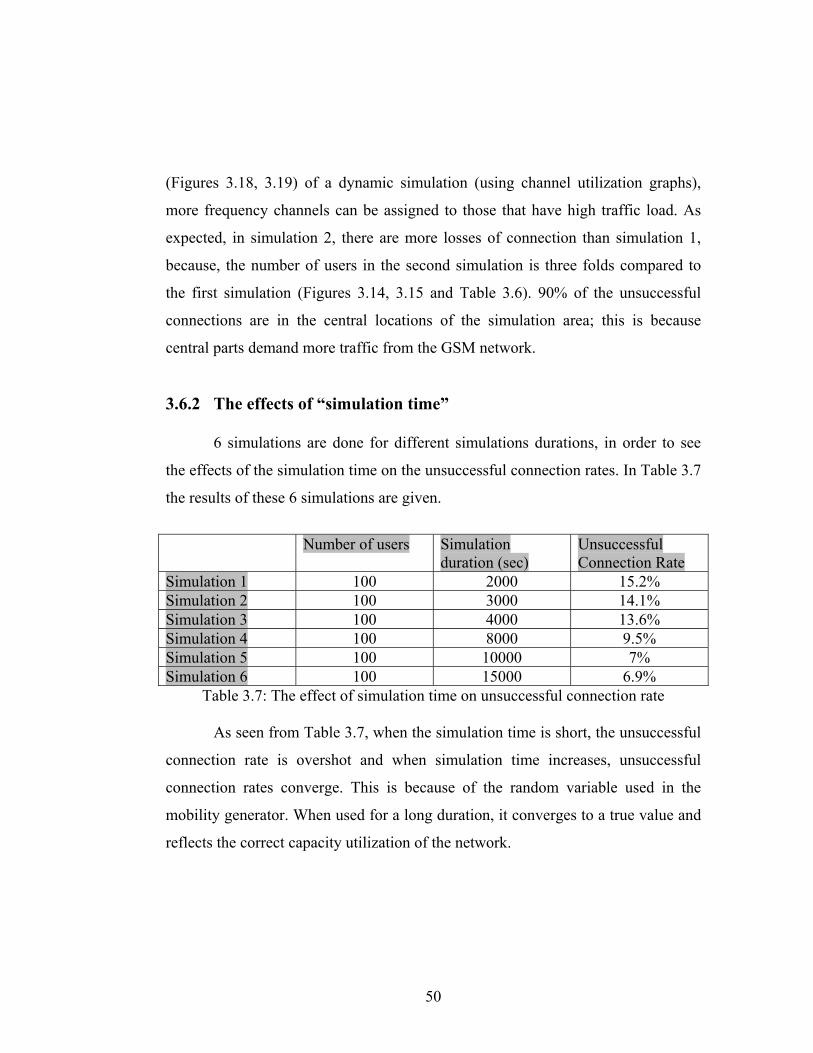
3.6.2 The effects of “simulation time”
6 simulations are done for different simulations durations, in order to see
the effects of the simulation time on the unsuccessful connection rates. In Table 3.7
the results of these 6 simulations are given.
Number of users Simulation
duration (sec) Unsuccessful Connection Rate
Simulation 1 100 2000 15.2% Simulation 2 100 3000 14.1% Simulation 3 100 4000 13.6% Simulation 4 100 8000 9.5% Simulation 5 100 10000 7% Simulation 6 100 15000 6.9%
Table 3.7: The effect of simulation time on unsuccessful connection rate
As seen from Table 3.7, when the simulation time is short, the unsuccessful
connection rate is overshot and when simulation time increases, unsuccessful
connection rates converge. This is because of the random variable used in the
mobility generator. When used for a long duration, it converges to a true value and
reflects the correct capacity utilization of the network.
51
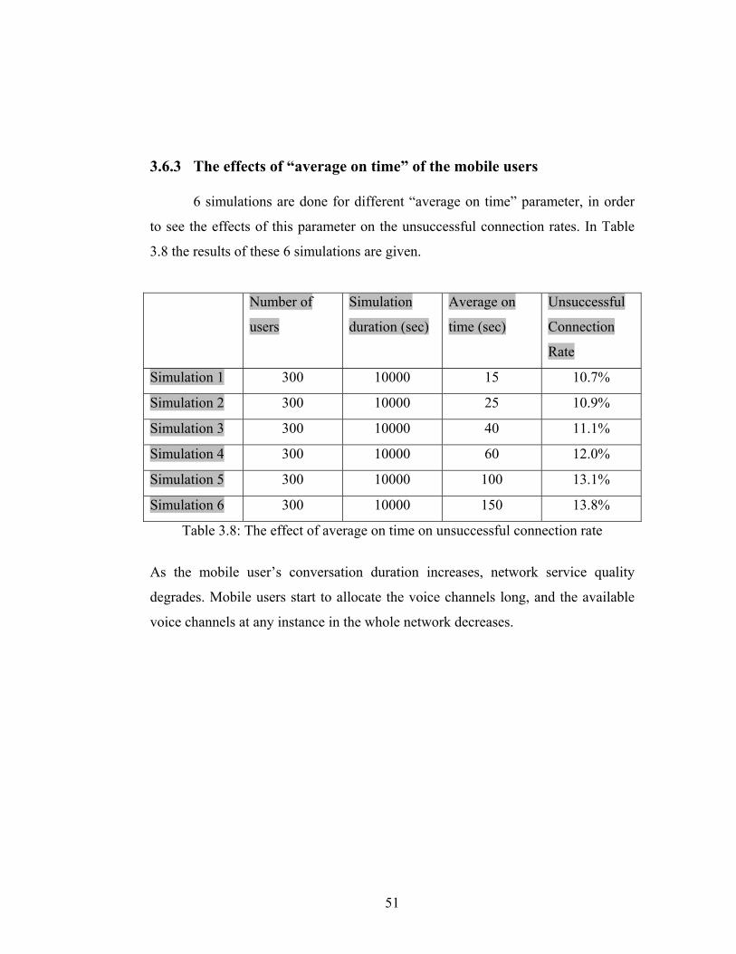
3.6.3 The effects of “average on time” of the mobile users
6 simulations are done for different “average on time” parameter, in order
to see the effects of this parameter on the unsuccessful connection rates. In Table
3.8 the results of these 6 simulations are given.
Number of
users
Simulation
duration (sec)
Average on
time (sec)
Unsuccessful
Connection
Rate
Simulation 1 300 10000 15 10.7%
Simulation 2 300 10000 25 10.9%
Simulation 3 300 10000 40 11.1%
Simulation 4 300 10000 60 12.0%
Simulation 5 300 10000 100 13.1%
Simulation 6 300 10000 150 13.8%
Table 3.8: The effect of average on time on unsuccessful connection rate
As the mobile user’s conversation duration increases, network service quality
degrades. Mobile users start to allocate the voice channels long, and the available
voice channels at any instance in the whole network decreases.
52
Chapter 4 UMTS SIMULATION
In this chapter, a dynamic UMTS network simulator tool is explained. A
static simulator does not model the time-depending characteristics of UMTS
system, dynamic power control, mobile motions and dynamic call statistics of
mobile users. Therefore a dynamic simulation tool is needed to see the performance
of this wireless network accurately [12]. The tool is similar to the GSM network
simulator. Both of them are mobility simulators that imitate the mobile behavior of
the users and reflect the responses of these wireless networks due to this dynamic
changing in conditions. On the other hand, the main difference between UMTS and
GSM simulator is the importance of modeling and calculation of the interference in
the network. In addition to this, in UMTS there exist different data rate demands
that cause different signal-to-noise ratio requirements at the base and mobile
stations. Uplink8 and downlink9 conditions can be thought as in balance, so in this
UMTS network simulator, only uplink is modeled. Propagation simulations are
done similarly in both GSM and UMTS networks explained in the previous
sections. Uplink only modeling is an assumption, which omits the downlink
conditions in the UMTS system.
In fact, this simulator can be referred as a long-term dynamic simulator,
because it is an extended version of a static simulator. Static simulation’s snapshots
are linked together in the time scale. Each mobile has two important time-related 8 Uplink is the connection from mobile to base station 9 Downlink is the connection from base to mobile station
53
characteristics, movement and call activity. Mobility behavior is designed
carefully, because the intended traffic distribution is non-homogenous. The
probability of mobile passing through any particular simulation space is non-
homogenous. This kind of a model can support variation of the mobile’s data rates
during a call. Call activity can be modeled by exponential traffic, that, every
mobile is set to on or off modes during the simulation time. On the average, each
mobile on/off periods fits to an exponential distribution. The traffic model is the
same as the GSM simulator case, explained in Chapter 3.
A long-term dynamic model is expected to operate in large time steps (1s –
20s) [12]. In the simulation model, there is no-explicit signal level fading and
therefore no explicit power control. However, at every time step, the system power
balancing is triggered, accounting for changes in path loss between mobile and the
base stations as well as initiation or termination of calls. During the power-
balancing algorithm, changes in soft handover status are also calculated and taken
into account. The status of the base station’s average transmitted power can be
utilized to admit or reject new calls.
4.1 UMTS Overview
In response to the growing demand, Universal Mobile Telecommunications
System signals to move into third generation (3G) of mobile networks. UMTS uses
Code Division Multiple Access (CDMA) as medium access layer. In CDMA, every
user will be allocated the entire spectrum all of the time, in opposite to GSM
networks that use TDMA and FDMA.
CDMA uses unique spreading code signal to spread the base-band data. In
order to spread the data, the spreading code signal must have larger rate. The rate
of this signal is called chip rate and denoted by W10. At the receiver, there is a
10 W is the chip rate, which is equal to 3.84MHz in UMTS
54
signal, which consists of different coded signals overlapped at the same frequency
band [13].
The channel consists of same frequency band signals overlapped in time.
Using unique codes at the transmitter, the receiver can de-correlate the wanted
signal.
The interference acts as noise at the receiver. Optimally, the codes are
100% orthogonal, but in a real case, they are not. In order to have a large number
of these orthogonal coding signals, the length of the code must be very large and it
is not practical. The interference is due to this problem of coding signals. The
receiver cannot de-correlate the wanted signal when interference is high. System
capacity and call quality is very much dependent on the interference level. Power
control process is deployed in UMTS to struggle the effects of the interference. It is
used to limit the transmit powers of both the mobile and the base station, while
maintaining the required level for good call quality.
55
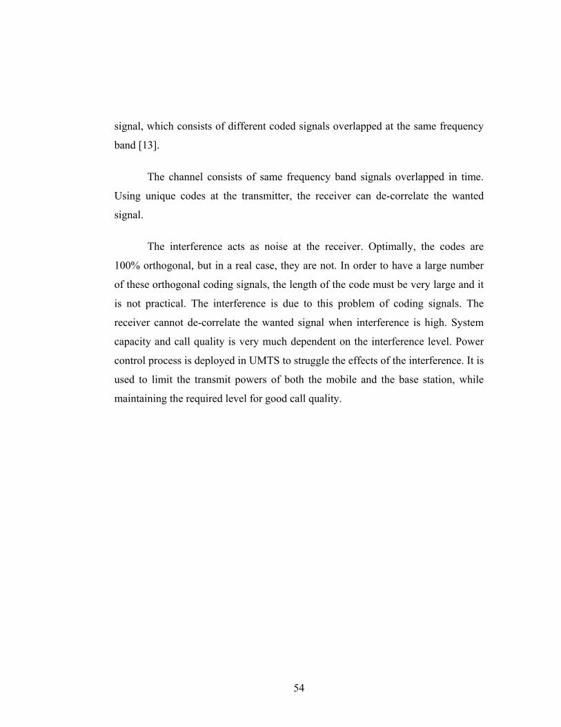
4.2 Configuration Parameters and Performance Metrics
In the initialization part of the program, the UMTS network related
parameters, base and mobile station parameters, propagation simulation results and
the parameters needed for the mobility simulator are loaded to the dynamic UMTS
simulator tool. The parameters are tabulated in Table 4.1.
Table 4.1: Configuration parameters of UMTS simulator
After, loading the parameters, the link level simulation results are inserted
to the tool structure. In this thesis, ‘ITU’s Pedestrian A’ link model [14] for UMTS
is used. The model is used to extract Eb/No11 requirements for different service
demands. Service demand in UMTS changes with different data rate and user
speed. Link level simulation results also consists of average transmit power rise
with respect to different mobile speeds, SHO gain with respect to user speeds and
the signal power difference between the best server link and the second best server
link. In addition, activity factors for different data rates and orthogonality factor for
different mobile speeds are implemented in ITU’s recommendation [14].
11 Eb/No is bit energy per noise density
56
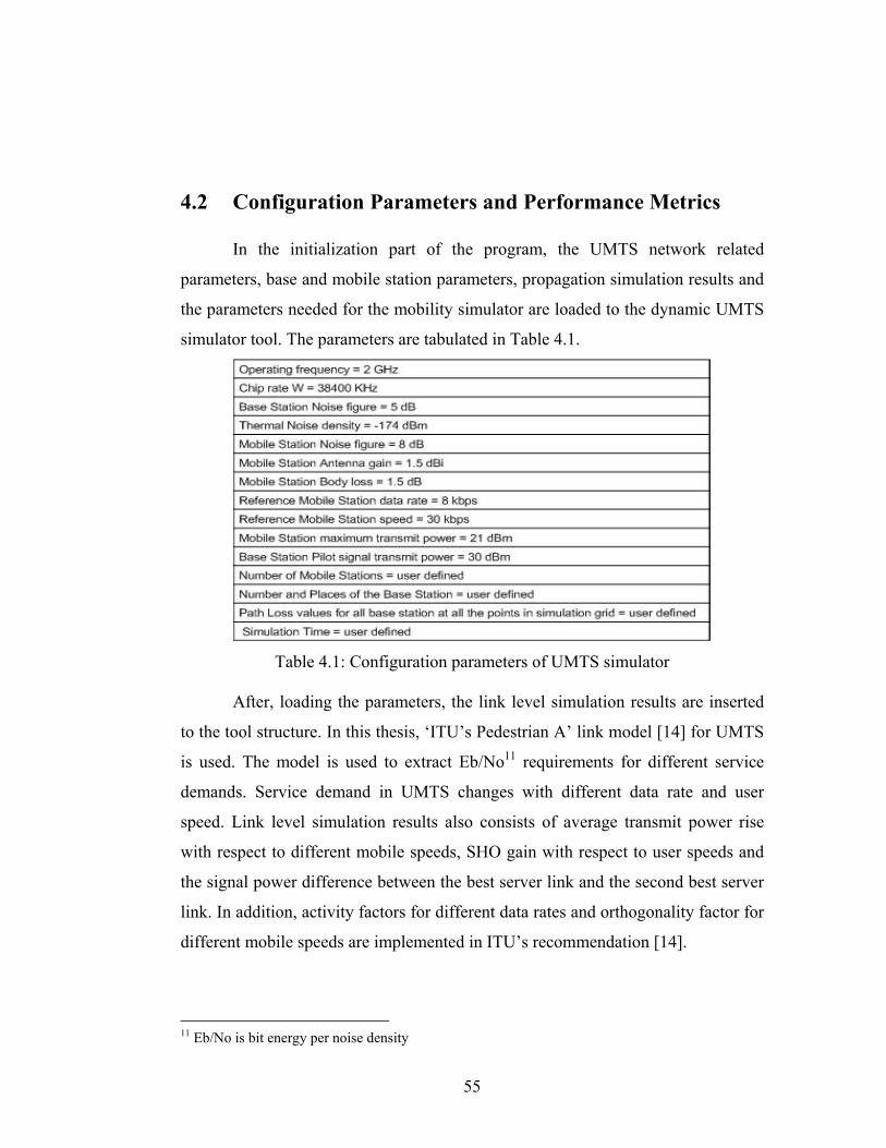
Eb/No value is an important parameter in CDMA networks. It represents
the average bit energy to noise-density ratio requirement. This requirement varies
with different data rates of the mobile users. UMTS, which uses CDMA as medium
access layer, inference can be modeled as noise (No) because all of the users use
the same frequency channel but with different codes. The codes must be 100%
orthogonal otherwise, interference happens. As the data rate demand and the speed
of the mobile increases, the Eb/No requirement for a successful connection
increases. This property is depicted in Figure 4.1.
Eb/No requirement for different data rates
0
2
4
6
8
0 50 100 150
speed (km/h)
Eb/N
o (d
B)
datarate =8kbpsdatarate =12.2 kbpsdatarate =64 kbpsdatarate =144 kbpsdatarate =512 kbps
Figure 4.1: Eb/No requirement versus data rate and speed.
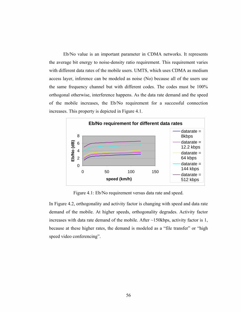
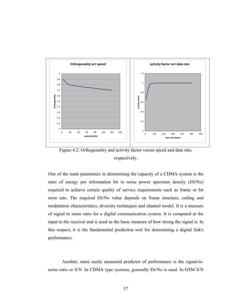
In Figure 4.2, orthogonality and activity factor is changing with speed and data rate
demand of the mobile. At higher speeds, orthogonality degrades. Activity factor
increases with data rate demand of the mobile. After ~150kbps, activity factor is 1,
because at these higher rates, the demand is modeled as a “file transfer” or “high
speed video conferencing”.
57
Orthogonality wrt speed
0
0.1
0.2
0.3
0.4
0.5
0.6
0.7
0.8
0.9
1
0 20 40 60 80 100 120 140
speed (km/h)
Ort
hogo
nalit
y
activity factor wrt data rate
0
0.2
0.4
0.6
0.8
1
1.2
0 100 200 300 400 500 600
data rate (kbps)ac
tivity
fact
or
Figure 4.2: Orthogonality and activity factor versus speed and data rate,
respectively.
One of the main parameters in determining the capacity of a CDMA system is the
ratio of energy per information bit to noise power spectrum density (Eb/No)
required to achieve certain quality of service requirements such as frame or bit
error rate. The required Eb/No value depends on frame structure, coding and
modulation characteristics, diversity techniques and channel model. It is a measure
of signal to noise ratio for a digital communication system. It is computed at the
input to the receiver and is used as the basic measure of how strong the signal is. In
this respect, it is the fundamental prediction tool for determining a digital link's
performance.
Another, more easily measured predictor of performance is the signal-to-
noise ratio or S/N. In CDMA type systems, generally Eb/No is used. In GSM S/N
58
is used, as a signal quality metric. Eb/No can be converted to S/N by the fallowing
formulas (4.1) and (4.2):
*S Eb dN No B
= (4.1)
* *N k T B= (4.2) where,
d: Data rate
B: Bandwidth
N: Noise
k: Boltzmann's constant = 1.380650x10⁻²³ J/K,
T: Effective temperature in Kelvin, and = 290K,
B: Receiver bandwidth = 1MHz.
N= (1.380650x10⁻²³ J/K) * (290K) *(1MHz) = 4x10-15 W = 4x10-12mW = -114dBm
By using this conversion, the required signal power can be calculated. This
is how much power the receiver must have at its input. To determine the real
transmitter power, the path loss must be added. The receivers are designed taking
into account this noise, in a CDMA network. This noise has a frequency spectrum
that is continuous and uniform over a specified frequency band. White noise has
equal power per hertz over the specified frequency band. In addition to this noise,
there exists interference due to imperfect orthogonal codes. This power value is
added to the noise, degrading call quality at the receiver.
In GSM simulation, minimum required received signal power for a mobile
user to access the network is constant because all the users use the same data rate.
On the other hand, in UMTS the minimum required signal power for a successful
connection is determined by the Eb/No requirement and interference at the terminal
depending on the data rate, speed and othagonality of the codes. Code Division
Multiple Access (CDMA) systems are well known to be interference limited and to
59
require power control to counteract the effects of the near-far problem and slow
shadow fading. In addition, third generation mobile radio systems based on
CDMA, such us UMTS, use fast power control which is able to increase capacity
by compensating radio channel variations due to multi-path fading for users
moving at a low, even moderate speed [15, 23].
Fast power control mechanism is deployed in UMTS because the
adjustment of the transmit powers of both the base and the mobile stations is
crucial. Unnecessary amount of transmit power of mobile or the base stations
degrades the capacity and the performance of the CDMA networks. In UMTS, the
interference is modeled as noise and the receivers can distinguish the same
frequency signals using orthogonal codes if the received powers are nearly the
same at the terminal. However if a signal dominates the receiver with vast power,
receiver cannot demodulate the data needed from the signals that have the same
frequency. In this scheme, so many variations of the transmit powers cause an
average increase in noise at the terminals. An average amount power must be
added to the transmit powers of the mobile units. The value is obtained from the
“ITU’s pedestrian A” tables. Orthogonality must also be modeled in calculating the
interference coming from the other terminals that are also communicating. The
othogonality factor depends on the mobile terminal speed and it is obtained from
the link level simulation results.
Handover occurs when a call has to be passed from one cell to another as
the user moves between cells. In a traditional "hard" handover, the connection to
the current cell is broken, and then the connection to the new cell is made. This is
known as a "break-before-make" handover. Since all cells in CDMA use the same
frequency, it is possible to make the connection to the new cell before leaving the
current cell. This is known as a "make-before-break" or "soft" handover. Soft
handovers require less power, which reduces interference and increases capacity.
Mobile can be connected to more than two BTS [13].
60
When a mobile terminal is in soft handover, it is actually communicating
with more than one base station. The received signals at the multiple base stations
are compared and the best of those signals is used. By this way, UMTS networks
advantages the performance in the uplink. In addition to this, if there are more than
one used links for only one communication, at the receiver the Eb/No requirement
decreases. The SHO12 gain is subtracted from the normal Eb/No requirement. In
GSM there is an active set that is determined by the received signal strengths and
the mobile user handovers between the base stations that are in the active set.
Conversely, in UMTS the mobile terminal setups links to all off the base stations in
the active set. These values calculated from the link level simulation results,
obtained by ITU pedestrian A, are different for each mobile station that
communicates in uplink. Different mobiles can demand different services with
varying physical speeds.
4.3 UMTS Mobility Simulator Algorithm
The UMTS simulator program tries to assign appropriate mobile station
transmit powers. Program uses a convergence loop and iterates a number of times,
reaching the convergence criteria. The time resolution of the simulator is similar to
the GSM network simulator and is in the order of seconds, which is user adjustable.
At every iteration step, the base station sensitivities are calculated and compared
with the previous iteration’s sensitivity value. If there is a small difference, the
convergence criterion is satisfied and simulator advances to the next simulation
instance. At every simulation instance, the mobiles are moved. Base station
sensitivity is the required signal power that the base station needs for a successful
uplink connection. The simulator’s block diagram is shown in Figure 4.3.
12 SHO is Soft Handover
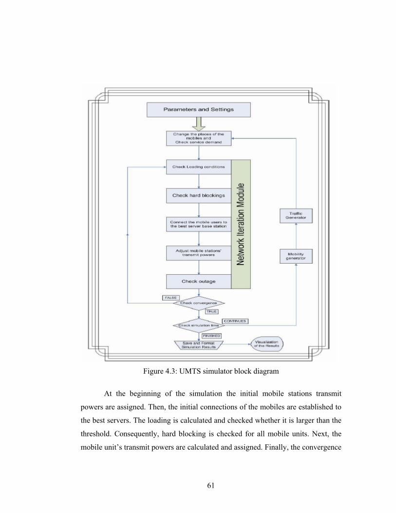
61
Figure 4.3: UMTS simulator block diagram
At the beginning of the simulation the initial mobile stations transmit
powers are assigned. Then, the initial connections of the mobiles are established to
the best servers. The loading is calculated and checked whether it is larger than the
threshold. Consequently, hard blocking is checked for all mobile units. Next, the
mobile unit’s transmit powers are calculated and assigned. Finally, the convergence
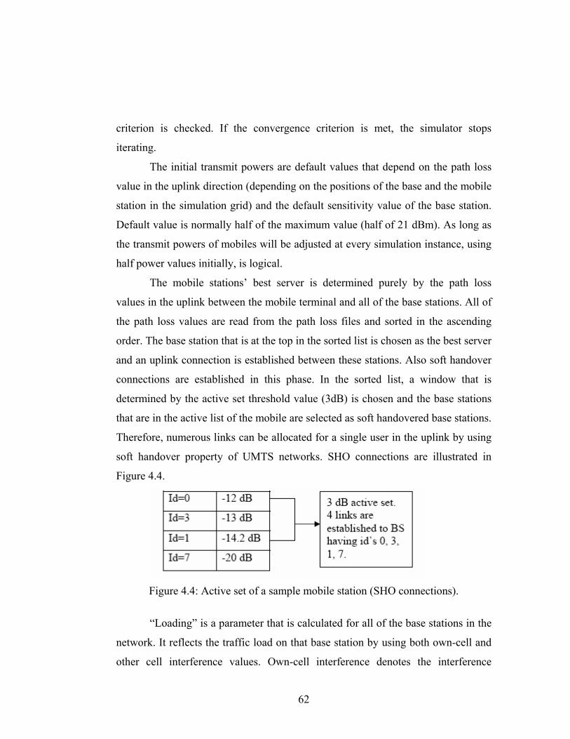
62
criterion is checked. If the convergence criterion is met, the simulator stops
iterating.
The initial transmit powers are default values that depend on the path loss
value in the uplink direction (depending on the positions of the base and the mobile
station in the simulation grid) and the default sensitivity value of the base station.
Default value is normally half of the maximum value (half of 21 dBm). As long as
the transmit powers of mobiles will be adjusted at every simulation instance, using
half power values initially, is logical.
The mobile stations’ best server is determined purely by the path loss
values in the uplink between the mobile terminal and all of the base stations. All of
the path loss values are read from the path loss files and sorted in the ascending
order. The base station that is at the top in the sorted list is chosen as the best server
and an uplink connection is established between these stations. Also soft handover
connections are established in this phase. In the sorted list, a window that is
determined by the active set threshold value (3dB) is chosen and the base stations
that are in the active list of the mobile are selected as soft handovered base stations.
Therefore, numerous links can be allocated for a single user in the uplink by using
soft handover property of UMTS networks. SHO connections are illustrated in
Figure 4.4.
Figure 4.4: Active set of a sample mobile station (SHO connections).
“Loading” is a parameter that is calculated for all of the base stations in the
network. It reflects the traffic load on that base station by using both own-cell and
other cell interference values. Own-cell interference denotes the interference
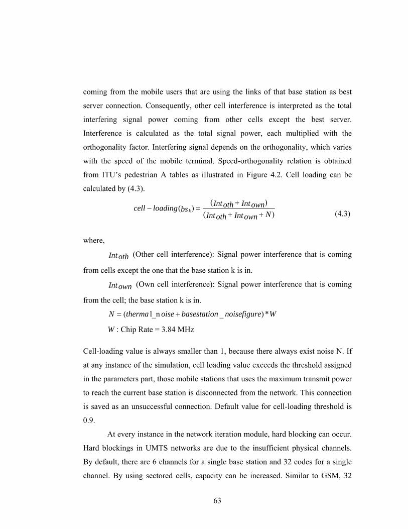
63
coming from the mobile users that are using the links of that base station as best
server connection. Consequently, other cell interference is interpreted as the total
interfering signal power coming from other cells except the best server.
Interference is calculated as the total signal power, each multiplied with the
orthogonality factor. Interfering signal depends on the orthogonality, which varies
with the speed of the mobile terminal. Speed-orthogonality relation is obtained
from ITU’s pedestrian A tables as illustrated in Figure 4.2. Cell loading can be
calculated by (4.3).
( )
( )( )k
Int Intoth owncell loading bs NInt Intoth own
+− =
+ + (4.3)
where,
Intoth (Other cell interference): Signal power interference that is coming
from cells except the one that the base station k is in.
Intown (Own cell interference): Signal power interference that is coming
from the cell; the base station k is in.
( l_n _ ) *N therma oise basestation noisefigure W= +
W : Chip Rate = 3.84 MHz Cell-loading value is always smaller than 1, because there always exist noise N. If
at any instance of the simulation, cell loading value exceeds the threshold assigned
in the parameters part, those mobile stations that uses the maximum transmit power
to reach the current base station is disconnected from the network. This connection
is saved as an unsuccessful connection. Default value for cell-loading threshold is
0.9.
At every instance in the network iteration module, hard blocking can occur.
Hard blockings in UMTS networks are due to the insufficient physical channels.
By default, there are 6 channels for a single base station and 32 codes for a single
channel. By using sectored cells, capacity can be increased. Similar to GSM, 32
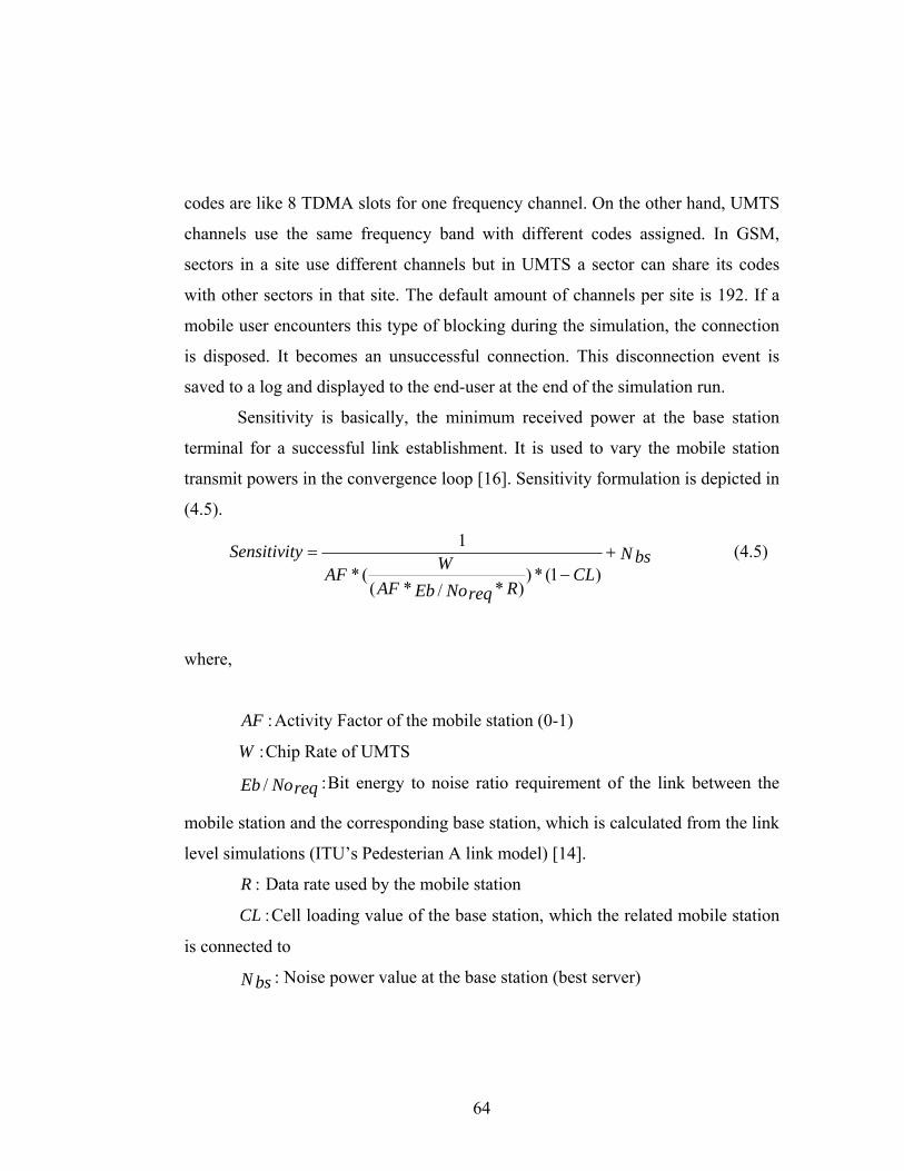
64
codes are like 8 TDMA slots for one frequency channel. On the other hand, UMTS
channels use the same frequency band with different codes assigned. In GSM,
sectors in a site use different channels but in UMTS a sector can share its codes
with other sectors in that site. The default amount of channels per site is 192. If a
mobile user encounters this type of blocking during the simulation, the connection
is disposed. It becomes an unsuccessful connection. This disconnection event is
saved to a log and displayed to the end-user at the end of the simulation run.
Sensitivity is basically, the minimum received power at the base station
terminal for a successful link establishment. It is used to vary the mobile station
transmit powers in the convergence loop [16]. Sensitivity formulation is depicted in
(4.5).
1
* ( ) * (1 )( * * )/
Sensitivity N bsWAF CLAF REb Noreq
= +−
(4.5)
where,
:AF Activity Factor of the mobile station (0-1)
:W Chip Rate of UMTS
:/Eb Noreq Bit energy to noise ratio requirement of the link between the
mobile station and the corresponding base station, which is calculated from the link
level simulations (ITU’s Pedesterian A link model) [14].
:R Data rate used by the mobile station
:CL Cell loading value of the base station, which the related mobile station
is connected to
N bs : Noise power value at the base station (best server)
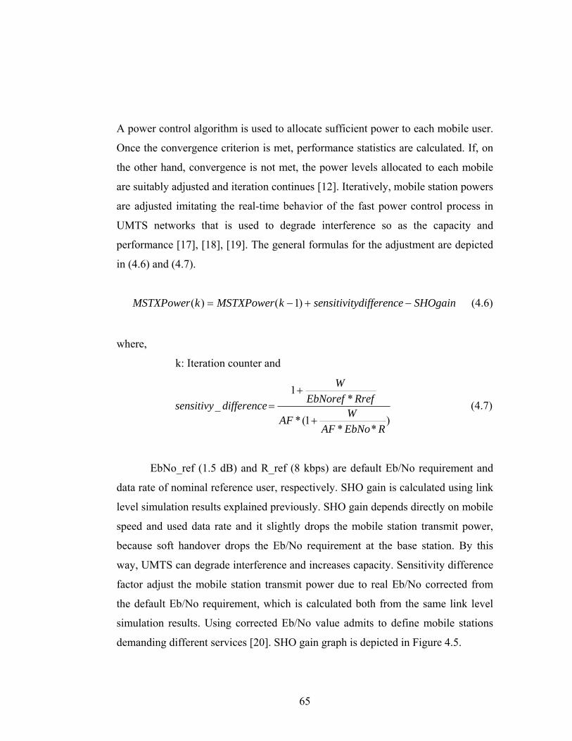
65
A power control algorithm is used to allocate sufficient power to each mobile user.
Once the convergence criterion is met, performance statistics are calculated. If, on
the other hand, convergence is not met, the power levels allocated to each mobile
are suitably adjusted and iteration continues [12]. Iteratively, mobile station powers
are adjusted imitating the real-time behavior of the fast power control process in
UMTS networks that is used to degrade interference so as the capacity and
performance [17], [18], [19]. The general formulas for the adjustment are depicted
in (4.6) and (4.7).
( ) ( 1)MSTXPower k MSTXPower k sensitivitydifference SHOgain= − + − (4.6)
where,
k: Iteration counter and
)
**1(*
*1
_
REbNoAFWAF
RrefEbNorefW
differencesensitivy+
+= (4.7)
EbNo_ref (1.5 dB) and R_ref (8 kbps) are default Eb/No requirement and
data rate of nominal reference user, respectively. SHO gain is calculated using link
level simulation results explained previously. SHO gain depends directly on mobile
speed and used data rate and it slightly drops the mobile station transmit power,
because soft handover drops the Eb/No requirement at the base station. By this
way, UMTS can degrade interference and increases capacity. Sensitivity difference
factor adjust the mobile station transmit power due to real Eb/No corrected from
the default Eb/No requirement, which is calculated both from the same link level
simulation results. Using corrected Eb/No value admits to define mobile stations
demanding different services [20]. SHO gain graph is depicted in Figure 4.5.
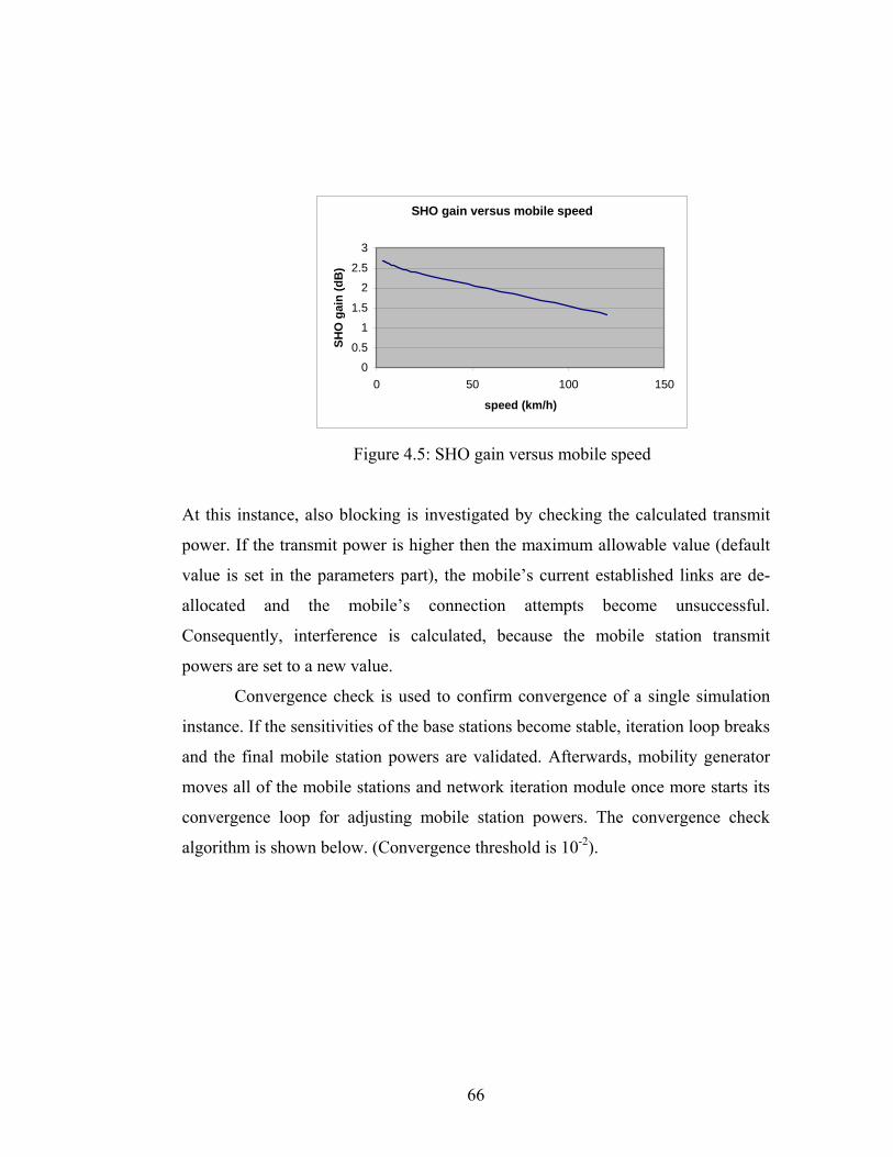
66
SHO gain versus mobile speed
0
0.5
1
1.5
2
2.5
3
0 50 100 150
speed (km/h)
SHO
gai
n (d
B)
Figure 4.5: SHO gain versus mobile speed
At this instance, also blocking is investigated by checking the calculated transmit
power. If the transmit power is higher then the maximum allowable value (default
value is set in the parameters part), the mobile’s current established links are de-
allocated and the mobile’s connection attempts become unsuccessful.
Consequently, interference is calculated, because the mobile station transmit
powers are set to a new value.
Convergence check is used to confirm convergence of a single simulation
instance. If the sensitivities of the base stations become stable, iteration loop breaks
and the final mobile station powers are validated. Afterwards, mobility generator
moves all of the mobile stations and network iteration module once more starts its
convergence loop for adjusting mobile station powers. The convergence check
algorithm is shown below. (Convergence threshold is 10-2).
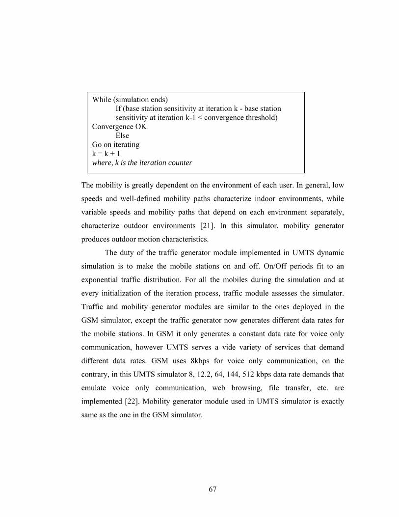
67
The mobility is greatly dependent on the environment of each user. In general, low
speeds and well-defined mobility paths characterize indoor environments, while
variable speeds and mobility paths that depend on each environment separately,
characterize outdoor environments [21]. In this simulator, mobility generator
produces outdoor motion characteristics.
The duty of the traffic generator module implemented in UMTS dynamic
simulation is to make the mobile stations on and off. On/Off periods fit to an
exponential traffic distribution. For all the mobiles during the simulation and at
every initialization of the iteration process, traffic module assesses the simulator.
Traffic and mobility generator modules are similar to the ones deployed in the
GSM simulator, except the traffic generator now generates different data rates for
the mobile stations. In GSM it only generates a constant data rate for voice only
communication, however UMTS serves a vide variety of services that demand
different data rates. GSM uses 8kbps for voice only communication, on the
contrary, in this UMTS simulator 8, 12.2, 64, 144, 512 kbps data rate demands that
emulate voice only communication, web browsing, file transfer, etc. are
implemented [22]. Mobility generator module used in UMTS simulator is exactly
same as the one in the GSM simulator.
While (simulation ends) If (base station sensitivity at iteration k - base station sensitivity at iteration k-1 < convergence threshold)
Convergence OK Else
Go on iterating k = k + 1 where, k is the iteration counter
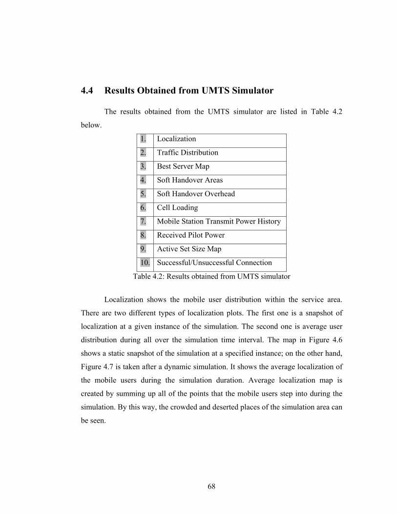
68
4.4 Results Obtained from UMTS Simulator
The results obtained from the UMTS simulator are listed in Table 4.2
below.
1. Localization
2. Traffic Distribution
3. Best Server Map
4. Soft Handover Areas
5. Soft Handover Overhead
6. Cell Loading
7. Mobile Station Transmit Power History
8. Received Pilot Power
9. Active Set Size Map
10. Successful/Unsuccessful Connection
Table 4.2: Results obtained from UMTS simulator
Localization shows the mobile user distribution within the service area.
There are two different types of localization plots. The first one is a snapshot of
localization at a given instance of the simulation. The second one is average user
distribution during all over the simulation time interval. The map in Figure 4.6
shows a static snapshot of the simulation at a specified instance; on the other hand,
Figure 4.7 is taken after a dynamic simulation. It shows the average localization of
the mobile users during the simulation duration. Average localization map is
created by summing up all of the points that the mobile users step into during the
simulation. By this way, the crowded and deserted places of the simulation area can
be seen.
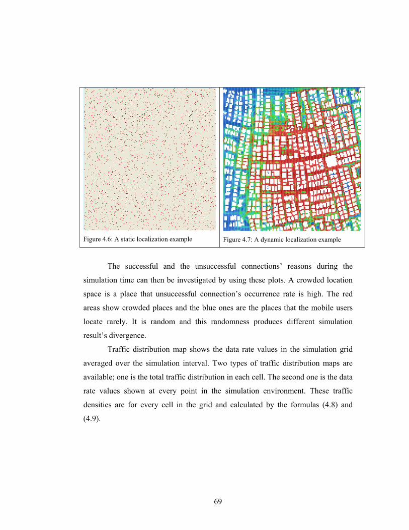
69
Figure 4.6: A static localization example Figure 4.7: A dynamic localization example
The successful and the unsuccessful connections’ reasons during the
simulation time can then be investigated by using these plots. A crowded location
space is a place that unsuccessful connection’s occurrence rate is high. The red
areas show crowded places and the blue ones are the places that the mobile users
locate rarely. It is random and this randomness produces different simulation
result’s divergence.
Traffic distribution map shows the data rate values in the simulation grid
averaged over the simulation interval. Two types of traffic distribution maps are
available; one is the total traffic distribution in each cell. The second one is the data
rate values shown at every point in the simulation environment. These traffic
densities are for every cell in the grid and calculated by the formulas (4.8) and
(4.9).
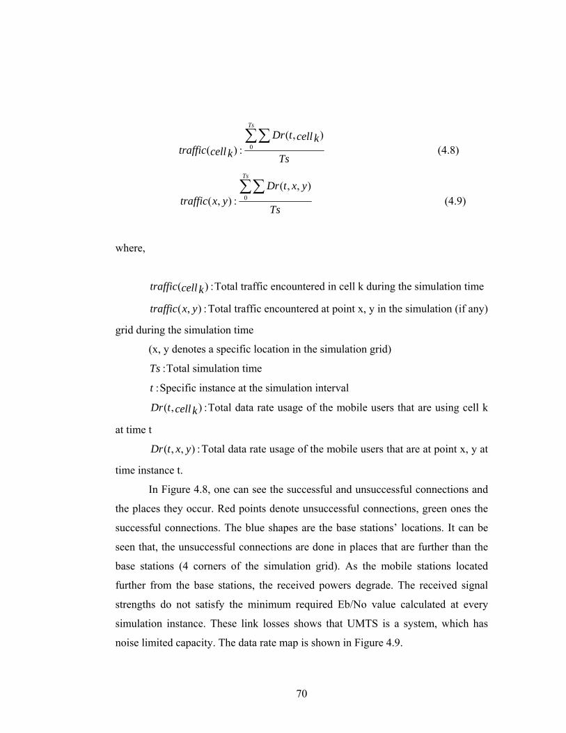
70
0( , )
( ) :
Ts
Dr t cell ktraffic cell k Ts
∑∑ (4.8)
0( , , )
( , ) :
Ts
Dr t x ytraffic x y
Ts
∑∑ (4.9)
where,
( ) :traffic cell k Total traffic encountered in cell k during the simulation time
( , ) :traffic x y Total traffic encountered at point x, y in the simulation (if any)
grid during the simulation time
(x, y denotes a specific location in the simulation grid)
:Ts Total simulation time
:t Specific instance at the simulation interval
( , ) :Dr t cell k Total data rate usage of the mobile users that are using cell k
at time t
( , , ) :Dr t x y Total data rate usage of the mobile users that are at point x, y at
time instance t.
In Figure 4.8, one can see the successful and unsuccessful connections and
the places they occur. Red points denote unsuccessful connections, green ones the
successful connections. The blue shapes are the base stations’ locations. It can be
seen that, the unsuccessful connections are done in places that are further than the
base stations (4 corners of the simulation grid). As the mobile stations located
further from the base stations, the received powers degrade. The received signal
strengths do not satisfy the minimum required Eb/No value calculated at every
simulation instance. These link losses shows that UMTS is a system, which has
noise limited capacity. The data rate map is shown in Figure 4.9.
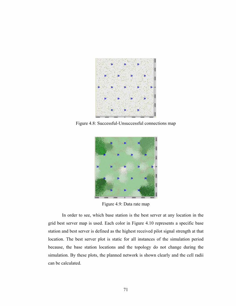
71
Figure 4.8: Successful-Unsuccessful connections map
Figure 4.9: Data rate map
In order to see, which base station is the best server at any location in the
grid best server map is used. Each color in Figure 4.10 represents a specific base
station and best server is defined as the highest received pilot signal strength at that
location. The best server plot is static for all instances of the simulation period
because, the base station locations and the topology do not change during the
simulation. By these plots, the planned network is shown clearly and the cell radii
can be calculated.
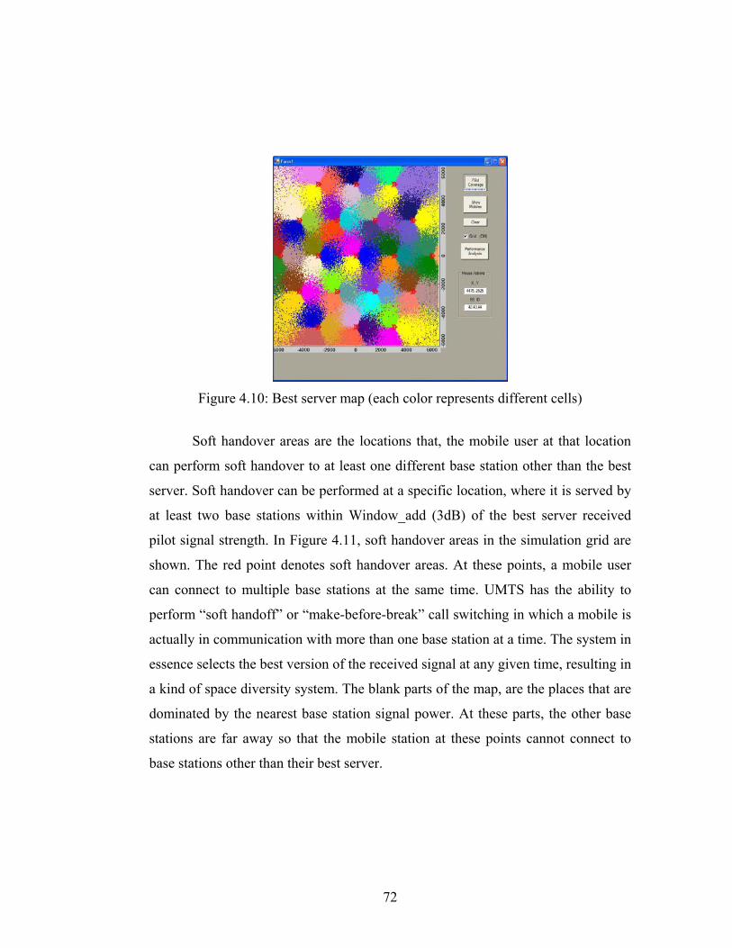
72
Figure 4.10: Best server map (each color represents different cells)
Soft handover areas are the locations that, the mobile user at that location
can perform soft handover to at least one different base station other than the best
server. Soft handover can be performed at a specific location, where it is served by
at least two base stations within Window_add (3dB) of the best server received
pilot signal strength. In Figure 4.11, soft handover areas in the simulation grid are
shown. The red point denotes soft handover areas. At these points, a mobile user
can connect to multiple base stations at the same time. UMTS has the ability to
perform “soft handoff” or “make-before-break” call switching in which a mobile is
actually in communication with more than one base station at a time. The system in
essence selects the best version of the received signal at any given time, resulting in
a kind of space diversity system. The blank parts of the map, are the places that are
dominated by the nearest base station signal power. At these parts, the other base
stations are far away so that the mobile station at these points cannot connect to
base stations other than their best server.
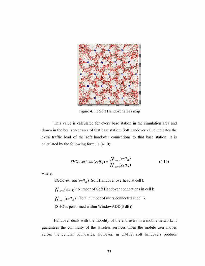
73
Figure 4.11: Soft Handover areas map
This value is calculated for every base station in the simulation area and
drawn in the best server area of that base station. Soft handover value indicates the
extra traffic load of the soft handover connections to that base station. It is
calculated by the following formula (4.10):
( )
( )( )
SHO
users
cell kSHOoverhead cell k cell kNN
= (4.10)
where,
( ) :SHOoverhead cell k Soft Handover overhead at cell k
( ) :SHO cell kN Number of Soft Handover connections in cell k
( ) :users cell kN Total number of users connected at cell k
(SHO is performed within WindowADD(3 dB))
Handover deals with the mobility of the end users in a mobile network. It
guarantees the continuity of the wireless services when the mobile user moves
across the cellular boundaries. However, in UMTS, soft handovers produce
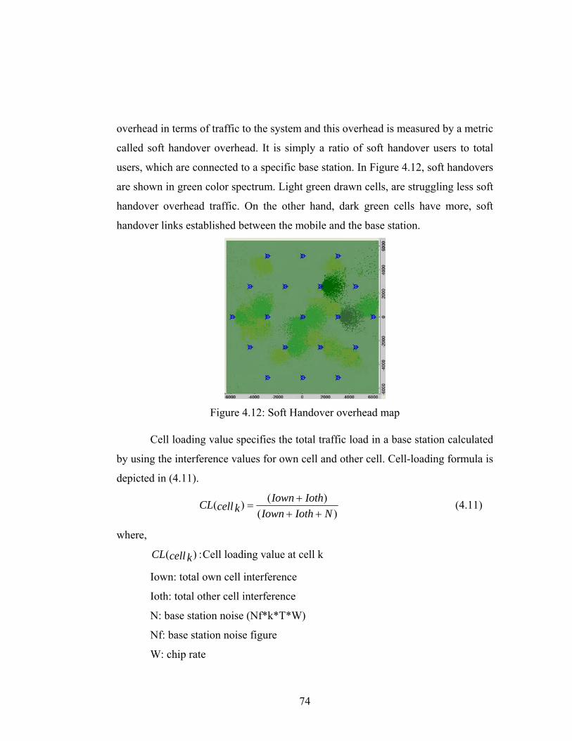
74
overhead in terms of traffic to the system and this overhead is measured by a metric
called soft handover overhead. It is simply a ratio of soft handover users to total
users, which are connected to a specific base station. In Figure 4.12, soft handovers
are shown in green color spectrum. Light green drawn cells, are struggling less soft
handover overhead traffic. On the other hand, dark green cells have more, soft
handover links established between the mobile and the base station.
Figure 4.12: Soft Handover overhead map
Cell loading value specifies the total traffic load in a base station calculated
by using the interference values for own cell and other cell. Cell-loading formula is
depicted in (4.11).
( )( )( )
Iown IothCL cell k Iown Ioth N+
=+ +
(4.11)
where,
( ) :CL cell k Cell loading value at cell k
Iown: total own cell interference
Ioth: total other cell interference
N: base station noise (Nf*k*T*W)
Nf: base station noise figure
W: chip rate
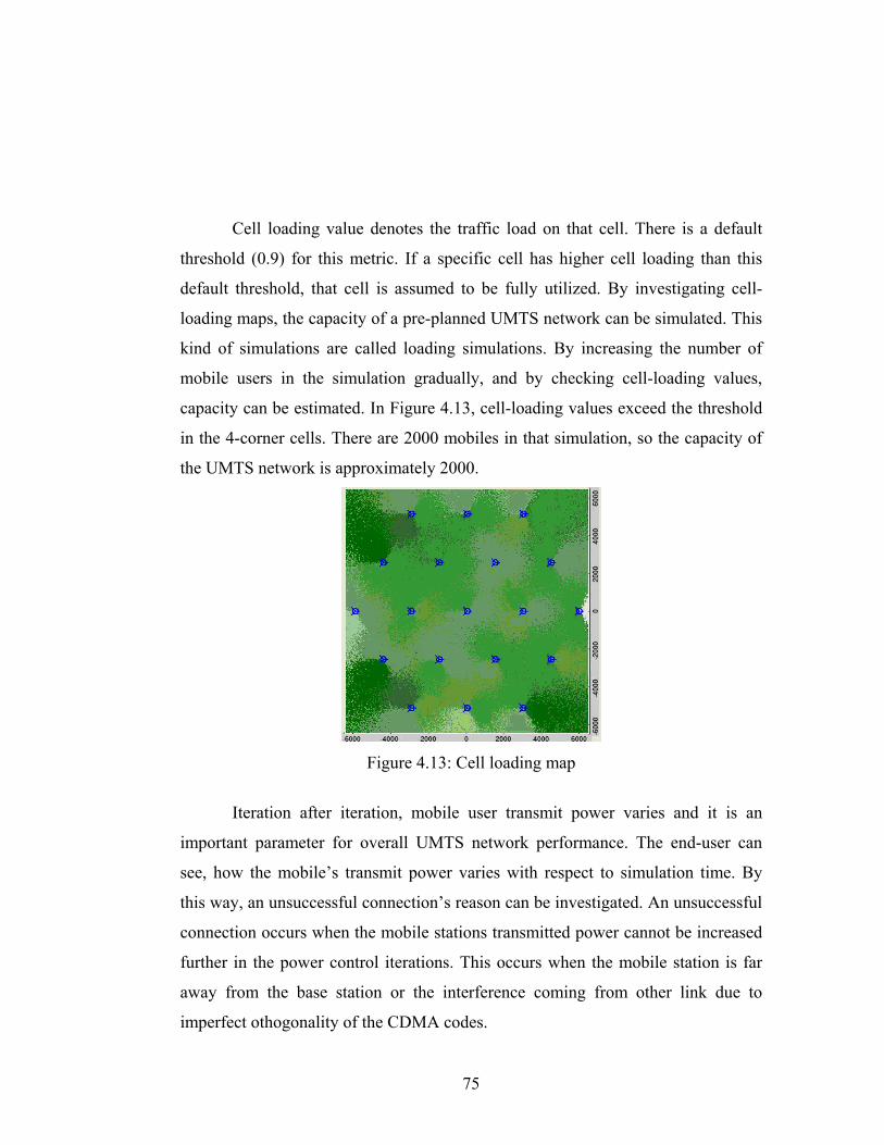
75
Cell loading value denotes the traffic load on that cell. There is a default
threshold (0.9) for this metric. If a specific cell has higher cell loading than this
default threshold, that cell is assumed to be fully utilized. By investigating cell-
loading maps, the capacity of a pre-planned UMTS network can be simulated. This
kind of simulations are called loading simulations. By increasing the number of
mobile users in the simulation gradually, and by checking cell-loading values,
capacity can be estimated. In Figure 4.13, cell-loading values exceed the threshold
in the 4-corner cells. There are 2000 mobiles in that simulation, so the capacity of
the UMTS network is approximately 2000.
Figure 4.13: Cell loading map
Iteration after iteration, mobile user transmit power varies and it is an
important parameter for overall UMTS network performance. The end-user can
see, how the mobile’s transmit power varies with respect to simulation time. By
this way, an unsuccessful connection’s reason can be investigated. An unsuccessful
connection occurs when the mobile stations transmitted power cannot be increased
further in the power control iterations. This occurs when the mobile station is far
away from the base station or the interference coming from other link due to
imperfect othogonality of the CDMA codes.
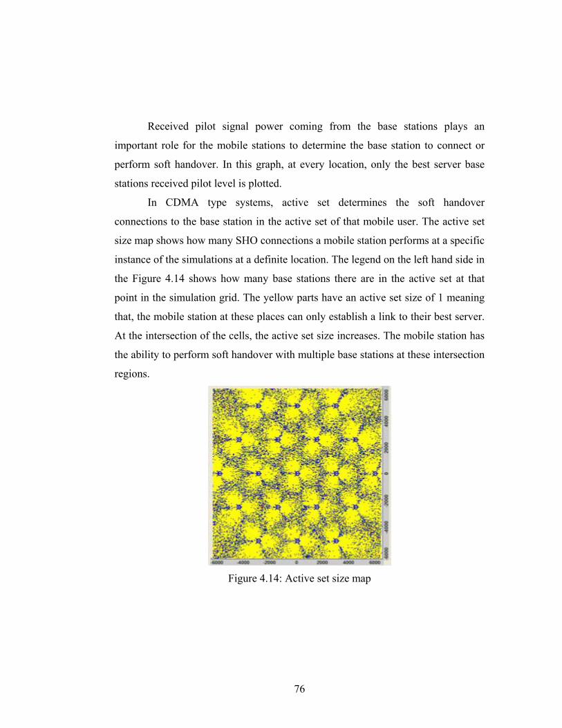
76
Received pilot signal power coming from the base stations plays an
important role for the mobile stations to determine the base station to connect or
perform soft handover. In this graph, at every location, only the best server base
stations received pilot level is plotted.
In CDMA type systems, active set determines the soft handover
connections to the base station in the active set of that mobile user. The active set
size map shows how many SHO connections a mobile station performs at a specific
instance of the simulations at a definite location. The legend on the left hand side in
the Figure 4.14 shows how many base stations there are in the active set at that
point in the simulation grid. The yellow parts have an active set size of 1 meaning
that, the mobile station at these places can only establish a link to their best server.
At the intersection of the cells, the active set size increases. The mobile station has
the ability to perform soft handover with multiple base stations at these intersection
regions.
Figure 4.14: Active set size map
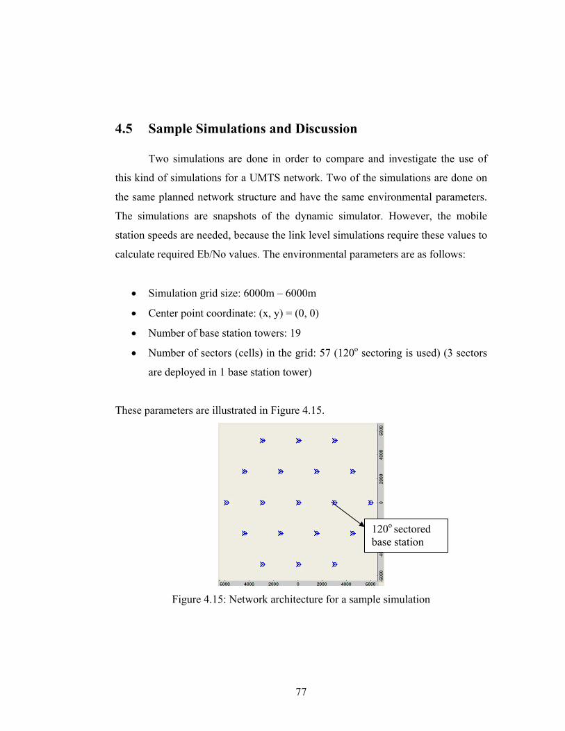
77
4.5 Sample Simulations and Discussion
Two simulations are done in order to compare and investigate the use of
this kind of simulations for a UMTS network. Two of the simulations are done on
the same planned network structure and have the same environmental parameters.
The simulations are snapshots of the dynamic simulator. However, the mobile
station speeds are needed, because the link level simulations require these values to
calculate required Eb/No values. The environmental parameters are as follows:
• Simulation grid size: 6000m – 6000m
• Center point coordinate: (x, y) = (0, 0)
• Number of base station towers: 19
• Number of sectors (cells) in the grid: 57 (120o sectoring is used) (3 sectors
are deployed in 1 base station tower)
These parameters are illustrated in Figure 4.15.
Figure 4.15: Network architecture for a sample simulation
120o sectored base station
78
The input data needed for the simulation is as follows:
Base station Data
The data consists of the following fields:
• x-y coordinates of the base stations: Stored in text files (19 BS - 57 sectors).
• Maximum transmit power for all traffic channels: 43 dBm
• Maximum transmit power per traffic link: 30 dBm
• Pilot power strength: 30 dBm
• Window ADD: -3 dB
Mobile station Data
• x-y coordinates of the base stations: Stored in text files
• Maximum and minimum transmit powers: 21 dBm, -50dBm
• Data Rates used by the mobile stations: Vary from one MS to another (8
kbps, 64 kbps, and 14.4 kbps). Stored in text files
• Ground speed: (5 km/h, 30 km/h, 50 km/h and 120 km/h)
Building Data and Propagation Simulation
This data is needed to make propagation simulations over the terrain and
give information to the mobility generator (Mobile users cannot enter buildings). In
this thesis, the propagation simulations are not investigated, but only used as inputs
to the mobility simulator. Okumura Hata model [7] is used for propagation
simulations with some random variation (deviation) around the calculated value.

79
Simulation I and II
Simulation I and II has nearly the same environment parameters. The
differences are the number, speed and the service demand (data rate) of mobile
stations, which are distributed in the simulation grid. The user distribution and their
properties are shown below:
Mobile stations Number Speed Service Demand
Simulation I 1200 10%: 120 km/h
20%: 50 km/h
30%: 30 km/h
40%: 5 km/h
50%: 8 kbps
30%: 64 kbps
20%: 14.4 kbps
Simulation II 3000 10%: 120 km/h
20%: 50 km/h
30%: 30 km/h
40%: 5 km/h
50%: 8 kbps
30%: 64 kbps
20%: 14.4 kbps
In both of the simulations the mobile stations are randomly (uniformly)
distributed over the simulation grid. 120 km/h mobile users refer to high-speed
vehicles, on the other hand 5 km/h users are pedestrians. Service demand varies
between 8 kbps to 14.4 kbps referring to a variation between only-voice calls to
high-speed file transfers. Simulation I is in a less crowded environment, because
number of mobile stations is less than simulation II. The reason for the difference
of the mobile station quantity is, by making these kinds of simulations, one can
estimate the effects of the traffic in a planned network. The variation of the speeds
and the service demands is because, the effects of these parameters are important
for a network supplier. A network provider should plan and re-plan the UMTS
network as the demands of the mobile users’ change, so using these kinds of
simulation tools is feasible and easy for a network administrator.
80
In simulation II, a crowded environment is simulated so, as long as UMTS
capacity is limited by noise (interference), more unsuccessful connections are
explainable. On the other hand, if the CDMA codes are perfectly orthogonal, the
system capacity will be thermal noise and physical channel quantity (number of
codes) limited. The available sectors are exactly the same for simulation I and II,
so as the total number of mobile users increase, the unsuccessful connection rate
increases. The total number of users in simulation II is more than two folds than the
users in simulation I, but the successful connections in case I are two folds than
case II. This makes the UMTS capacity non-linearly dependent on the traffic
demand, because when the users are more in the network, there exist additional
noise between the links and link losses occur. The sensitivity equation explained
previously satisfies this phenomenon. Sensitivity is the required Eb/No (analogous
to signal to noise ratio) value and it is directly proportional with CL (Cell loading)
[15]. Cell loading depends on the number connected users so, if there are more
users making communications in the network, the required Eb/No value is more.
The mobile users and the base stations have limited transmit powers, so the
mobiles that could not satisfy these criteria of required Eb/No struggles link losses.
There is no explicit limit to soft handover connections [17] in the network except
from required Eb/No threshold. The number of soft handover connections
increased linearly when going from simulation I to simulation II.
It can be seen from the numerical results (Figure 4.24) that large percentage of the
link losses occur when the mobile user is using high data rate or traveling with high
speeds. This phenomenon can be explained by the link level simulations and by
ITU’s pedestrian A table. As speed and data rate increases, the required clean
signal strength also increases. UMTS can support high data rates, so while planning
the CDMA network; this incident must be investigated carefully.
Figures 4.16 and 4.17 show that, the unsuccessful connections occur more
in simulation II (red points show unsuccessful connections). Figures 4.18, 4.19,
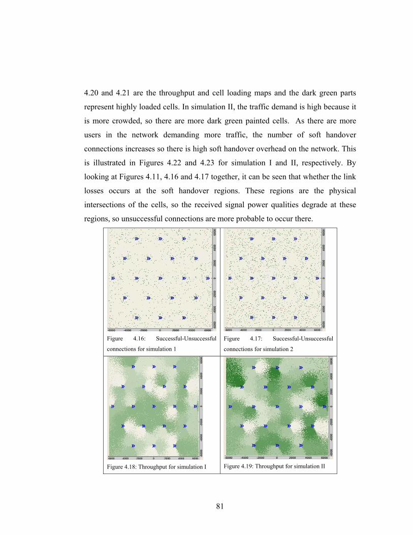
81
4.20 and 4.21 are the throughput and cell loading maps and the dark green parts
represent highly loaded cells. In simulation II, the traffic demand is high because it
is more crowded, so there are more dark green painted cells. As there are more
users in the network demanding more traffic, the number of soft handover
connections increases so there is high soft handover overhead on the network. This
is illustrated in Figures 4.22 and 4.23 for simulation I and II, respectively. By
looking at Figures 4.11, 4.16 and 4.17 together, it can be seen that whether the link
losses occurs at the soft handover regions. These regions are the physical
intersections of the cells, so the received signal power qualities degrade at these
regions, so unsuccessful connections are more probable to occur there.
Figure 4.16: Successful-Unsuccessful
connections for simulation 1
Figure 4.17: Successful-Unsuccessful
connections for simulation 2
Figure 4.18: Throughput for simulation I
Figure 4.19: Throughput for simulation II
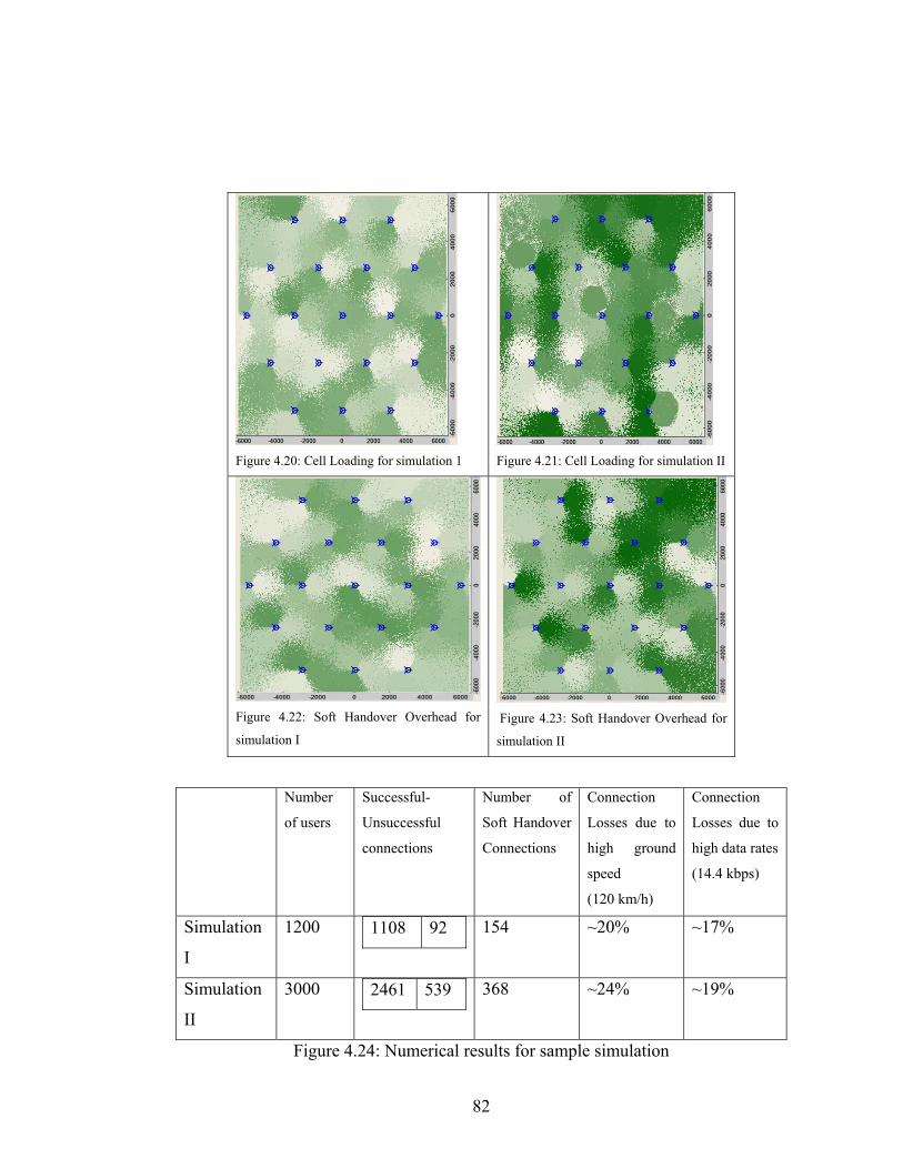
82
Figure 4.20: Cell Loading for simulation 1
Figure 4.21: Cell Loading for simulation II
Figure 4.22: Soft Handover Overhead for
simulation I
Figure 4.23: Soft Handover Overhead for
simulation II
Number
of users
Successful-
Unsuccessful
connections
Number of
Soft Handover
Connections
Connection
Losses due to
high ground
speed
(120 km/h)
Connection
Losses due to
high data rates
(14.4 kbps)
Simulation
I
1200 1108 92
154 ~20% ~17%
Simulation
II
3000 2461 539
368 ~24% ~19%
Figure 4.24: Numerical results for sample simulation
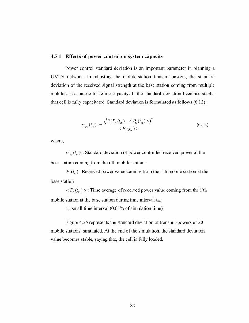
83
4.5.1 Effects of power control on system capacity
Power control standard deviation is an important parameter in planning a
UMTS network. In adjusting the mobile-station transmit-powers, the standard
deviation of the received signal strength at the base station coming from multiple
mobiles, is a metric to define capacity. If the standard deviation becomes stable,
that cell is fully capacitated. Standard deviation is formulated as follows (6.12):
2( ( ) ( ) )
( )( )
ri m ri mpc m i
ri m
E P t P tt
P tσ
− < >=
< > (6.12)
where,
( )pc m itσ : Standard deviation of power controlled received power at the
base station coming from the i’th mobile station.
( )ri mP t : Received power value coming from the i’th mobile station at the
base station
( )ri mP t< > : Time average of received power value coming from the i’th
mobile station at the base station during time interval tm.
tm: small time interval (0.01% of simulation time)
Figure 4.25 represents the standard deviation of transmit-powers of 20
mobile stations, simulated. At the end of the simulation, the standard deviation
value becomes stable, saying that, the cell is fully loaded.
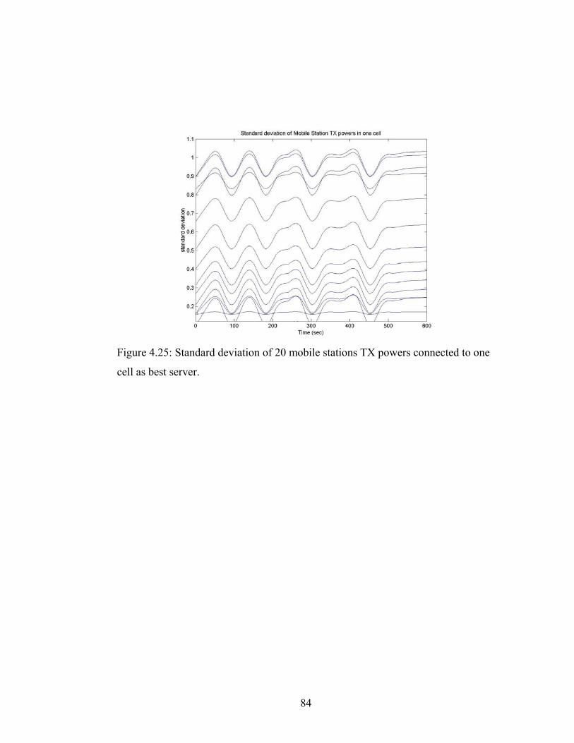
84
Figure 4.25: Standard deviation of 20 mobile stations TX powers connected to one
cell as best server.
85
Chapter 5 CONCLUSION AND FUTURE WORK
The aim of this thesis is to investigate the capacity and performance of two
wireless networks, GSM and UMTS. For this investigation to be accurate, mobility
simulations are needed. These simulators reflect the true performance and quality
of the network due to dynamic behavior of the mobile users. Mobile behavior of
the users must be well modeled to simulate the network realistically. For the
mobility modeling, a step-taking algorithm is used. The routes are not pre-
processed, so the algorithm is computationally efficient.
In simulating the GSM network handovers must be implemented in the
simulator, because disconnections during handovers crucially affect system quality.
GSM simulator models the network with a reasonable user traffic distribution and
an accurate signal propagation data on top of a real building map. The simulator
generates capacity and performance metrics due to different traffic loads and
subscriber mobility pattern.
The difference between GSM and UMTS simulators is the importance of
modeling and calculation of the interference in the network. In UMTS there are
different data rate demands. This divergence causes different signal-to-noise ratio
requirements at the base and mobile stations. The simulator can handle various data
rate demands. UMTS mobility simulator models dynamic power control, call
statistics and mobile movements. In addition soft handover capability of UMTS is
modeled and deployed to the simulator. In fact, UMTS simulator can be referred as
86
a long-term dynamic simulator. It is a continuous version of a static simulator,
because there is no explicit signal fading and power control. However, at every
instance of the simulation, the system power balancing is triggered due to changes
in mobile station locations and call statistics.
For the future work, the mobility generation algorithm may be extended to
calculate paths more realistically and efficient. This would make the program to
consider shortest paths to destination. Consequently, the simulating time would
decrease, resulting in the ability to perform longer simulations. In addition to this,
in the implantation of the UMTS simulator, the modeling of downlink
characteristics of this network is neglected. Only downlink is considered and
uplink is assumed to be in balance with downlink conditions. For the future work,
downlink simulations may be added to the program to consider uplink conditions.
87
APPENDIX Exponential traffic generation code public class ExponentialTraffic { public double ontime; public double offtime; public double rate; public int size; public double interval; public int rem; public bool started; ExponentialRandomVariable burstlen_; ExponentialRandomVariable Offtime_; public int next_start(int seed) { double t = interval; started = false; if(rem==0) { rem = (int)(burstlen_.get_val(seed) + 0.5); if(rem == 0) rem = 1; t += Offtime_.get_val(seed); started = true; } rem--; return((int)t); } public ExponentialTraffic() {
88
} public ExponentialTraffic(double _ontime,double _offtime,double _rate,int _size) { ontime = _ontime; offtime = _offtime; rate = _rate; size = _size; interval = (double)(size * 8)/(double)rate; Offtime_ = new ExponentialRandomVariable(offtime); burstlen_ = new ExponentialRandomVariable(ontime/interval); rem = 0; } } } GSM simulator code private void simulate() { dlg1.Show(); draw_map(); //dlg1.prog_reset(); DateTime now = DateTime.Now; Random rand = new Random((int) now.Millisecond); T_hand=Double.Parse(textBox1.Text); T_min=Double.Parse(textBox2.Text); trials=int.Parse(textBox5.Text); label9.Visible=false; hyst=6; progressBar1.Visible=true; progressBar1.Minimum = 1; progressBar1.Maximum = trials; progressBar1.Value = 1;

89
progressBar1.Step = 1; if(checkBox1.Checked) { fix_mobs=int.Parse(textBox3.Text); } if(checkBox2.Checked) uni=true; grids = new int[fix_mobs,2]; dest = new int[fix_mobs,2]; destbuf = new int[fix_mobs]; mstat = new double[fix_mobs,3]; mbuf = new int[fix_mobs,2]; mbufdir = new int[fix_mobs]; mbufdir2 = new bool[fix_mobs]; mbufdir3 = new int[fix_mobs,2]; mbufdir4 = new int[fix_mobs]; mbufdir5= new int[fix_mobs]; newly = new bool[fix_mobs]; startbuf = new int[fix_mobs]; channel_util = new int[txs.Length/3,trials]; for(int i=0;i<fix_mobs;i++) { mstat[i,0]=0;//Initially the radios are off. int xd=rand.Next(0,size_x); int yd=rand.Next(0,size_y); while(true) { if(grid[yd,xd]!=-99999 && yd<size_y && yd>0 && xd<size_x && xd>0) { dest[i,0]=xd; dest[i,1]=yd; mbuf[i,0]=-1; mbuf[i,1]=-1; mbufdir[i]=-1;
90
mbufdir2[i]=false; mbufdir3[i,0]=-1; mbufdir3[i,1]=-1; mbufdir5[i]=-1; destbuf[i]=-1; newly[i]=true; break; } else { xd=rand.Next(0,size_x); yd=rand.Next(0,size_y); } } } int mob_count=0; while(mob_count<fix_mobs) { int x=rand.Next(0,size_x); int y=rand.Next(0,size_y); if(grid[y,x]!=-99999) { grids[mob_count,0]=x; grids[mob_count,1]=y; mob_count++; } } for(int i=0;i<fix_mobs;i++) { mstat[i,2]=-1; } connected=0; handoffs=0; dropped=0; started=0;
91
init_traffic(); for(int t=0;t<trials;t++) { dlg1.textBox1.Text=(t+1).ToString(); DateTime nows = DateTime.Now; dlg1.textBox2.Text=nows.ToLongTimeString().ToString(); for(int i=0;i<fix_mobs;i++) { contour(); if(mstat[i,0]==1) { setup(i,t); mstat[i,1]--; if(mstat[i,1]==0 && mstat[i,2]!=-1) { mstat[i,0]=0; //dlg1.deprog(mstat[i,2]); chan_dealloc(int.Parse(mstat[i,2].ToString()),t); mstat[i,2]=-1; } } else { if(will_on(t,i)) { mstat[i,0]=1; //mstat[i,1]=calc_left(t,i); started++; } } move(grids[i,1],grids[i,0],i,t); location[grids[i,1],grids[i,0]]++; } for(int j=0;j<txs.Length/3;j++) { channel_util[j,t] = firsttxs[j] - txs[j,2];//kac tanesi dolu
92
} progressBar1.PerformStep(); } //dlg1.prog_reset(); MessageBox.Show("Simulation has ended. Now you can see the results.","GSM Analysis",MessageBoxButtons.OK,MessageBoxIcon.Information); dlg1.Hide(); write_report(); } private void setup(int im,int time) { int x=grids[im,0]; int y=grids[im,1]; int check=0; double src=0; if(mstat[im,2]==-1)//means very first beginning(Not Connected yet) { for(int i=0;i<7;i++) { if(search(x,y)[i,1]>T_min && txs[int.Parse((search(x,y)[i,0]).ToString()),2]>0) { src=search(x,y)[i,0]; mstat[im,2]=src; //dlg1.prog(mstat[im,2]); chan_alloc(int.Parse(src.ToString()),time); check=1; connected++; sector_info2[int.Parse(src.ToString()),1]++; suc_connection_map[y,x]++;
93
break; } } if(check==0) { //means not connected to any server dropped++; sector_info3[0,1]++; unsuc_connection_map[y,x]++; mstat[im,0]=0; mstat[im,1]=0; mstat[im,2]=-1; } } else//Already connected { int con=int.Parse(mstat[im,2].ToString()); int newcon=-1; if(rp[con,y,x]<T_hand)//recent base station's rp is below T-handoff { for(int i=0;i<7;i++) { if(search(x,y)[i,0]!=con) { if(search(x,y)[i,1]-rp[con,y,x]>=hyst && txs[int.Parse((search(x,y)[i,0]).ToString()),2]>0 && search(x,y)[i,1]>T_min) { newcon=int.Parse(search(x,y)[i,0].ToString()); break; } } } if(newcon!=-1)//handoff!!! { //dlg1.deprog(mstat[im,2]); chan_dealloc(con,time);//break before connecting to the new b.s. mstat[im,2]=newcon;
94
//dlg1.prog(mstat[im,2]); chan_alloc(newcon,time); handoffs++; sector_info2[newcon,0]++; suc_handoff_map[y,x]++; } if(newcon==-1 && rp[con,y,x]<T_min) { dropped++; sector_info3[0,0]++; unsuc_handoff_map[y,x]++; //dlg1.deprog(mstat[im,2]); chan_dealloc(con,time); mstat[im,0]=0; mstat[im,1]=0; mstat[im,2]=-1; } } } } UMTS simulator code System.Random rnd = new Random(); for(int i = 0;i<number_of_bs;i++) for(int j = 0;j<number_of_ms;j++) { linklossULM[i,j]=/*160;*/105+13*rnd.NextDouble(); //linklossDLM[i,j]=/*165;*/160+10*rnd.NextDouble(); } for(int i=0;i<number_of_bs;i++) for(int j=0;j<size_y;j++) for(int k=0;k<size_x;k++) {
95
pathlossUL[i,j,k]=/*145;*/100+13*rnd.NextDouble(); //pathlossDL[i,j,k]=/*150;*/135+10*rnd.NextDouble(); } IoM = new double[number_of_bs,number_of_ms]; CPICHM = new double[number_of_bs,number_of_ms]; CPICHEcIoM = new double[number_of_bs,number_of_ms]; reference_ms_EbNo = /*calc_ms_EbNoUL(reference_mobile_speed,reference_mobile_datarate)*/6.18; reference_ms_AFUL = calc_AF_UL(reference_mobile_datarate); reference_ms_AFDL = calc_AF_DL(reference_mobile_datarate); for(int i = 0;i<number_of_ms;i++) mobiles[i] = new Mobile(); for(int i = 0;i<number_of_bs;i++) bss[i] = new BaseStation(); //*****set MS and BS parameters***** // UNUTMA for(int i = 0;i<number_of_bs;i++) { bss[i].TxPower = new double[number_of_ms]; for(int j = 0;j<number_of_ms;j++) bss[i].TxPower[j] = -280; } UpdateChannel(); //********************************** //Create system performance parameters and its defaults defsysperf = new DefSystemPerf(); sysperf = new SystemPerf[number_of_bs]; for(int i=0;i<number_of_bs;i++) { sysperf[i] = new SystemPerf(); //Set system performance parameters to defaults sysperf[i].covth = defsysperf.covth; sysperf[i].inter = defsysperf.inter;
96
sysperf[i].mUL = defsysperf.mUL; sysperf[i].RUL = defsysperf.RUL; sysperf[i].SHO = defsysperf.SHO; } Initialize(); for(int i=0;i<number_of_ms;i++) { msTxPowerV[i]=mobiles[i].TxPower; } Itterate(); public static void Itterate() { while(true) { for(int i=0;i<number_of_bs;i++) oldThreshold[i] = sysperf[i].covth; iteration++; indexHL.Clear(); RlbUL(); for(int i=0;i<number_of_bs;i++) { newThreshold[i] = sysperf[i].covth; deltaCTnew[i] = Math.Abs(oldThreshold[i]-newThreshold[i]); } BestServerUL(); outageULold = (double[,])outageUL.Clone(); CalcMStx(); CalcIntUL(); //downlink starts CalcIntDL(); } }
97
BIBLIOGRAPHY
[1] Theodore S. Rappaport, “Wireless Communications, Principles & Practice”,
Prentice Hall, 1999
[2] Yi-Bing Lin, “No wires attached” Potentials IEEE, Volume: 14, Issue: 4, Oct.-
Nov. 1995
[3] A. Wacker, J. Laiho-Steffens, K. Sipila, M. Jasberg, 1999, “Static simulator for
studying WCDMA radio network planning issues”, IEEE 49th Veh. Tech. Conf.,
May 16 19, Houston, USA
[4] “GSM Overview”, 2002, Available at www.gsmworld.com
[5] NS network simulator user manual, Available at http://www.isi.edu/nsnam/ns
[6] Diran Nazarian, “Path finding in a Gaming Environment”, Catholic University
of America, 2002
[7] Y. Okumura Hata “Field Strength and its variability in UHF and VHF Land
Mobile Radio Service” Rev. Elec. Comm. Lab., Vol. 16,1968
[8] Shree Murty, J.J. Garcia-Luna-Aceves, “A more efficient path-finding
algorithm”, 2001
[9] Xiangguang Che, Hamalainen, S., Ryynanen, J., Moisio, M., “GPRS radio
network performance simulation and optimization with dynamic simulator”,
98
Communication Technology Proceedings, 2003. ICCT 2003. International
Conference, Volume: 2, 9-11 April 2003
[10] Knight, P., “Network planning using GSM and GSM based standards GSM
and PCN Enhanced Mobile Services”, IEE Colloquium on 30 Jan 1991
[11] da Silva, L., Belleli, T., Harris, S.P., “A decision support system for planning
GSM radio coverage GSM and PCN Enhanced Mobile Services”, IEE Colloquium
on, 30 Jan 1991
[12] Molkdar, D., Burley, S., Wallington, J., “Comparison between simulation and
analytical methods of UMTS air interface capacity dimensioning” Vehicular
Technology Conference, 2002. Proceedings. VTC 2002-Fall. 2002 IEEE 56th ,
Volume: 3 , 24-28 Sept. 2002, Pages:1596 - 1601 vol.3
[13] “UMTS and CDMA Overview” DRAFT, July 2002, Available at
http://www.umtsworld.com/
[14] “Guidelines for Evaluation of Radio Transmission Technologies for IMT-
2000”, ITU-R M.1225, 1997
[15] J. M. Romero-Jerez, M. Ruiz-García, C. Téllez-Labao, A. Díaz-Estrella Dpto.,
“Capacity Analysis of Multicell CDMA Networks with Fast Power Control under
Mutltipath Fading”, Tecnología Electrónica, E.T.S.I.
[16] Staehle, D., Leibnitz, K., Heck, K., “Effects of soft handover on the UMTS
downlink performance”, Vehicular Technology Conference, 2002. Proceedings.
99
VTC 2002-Fall. 2002 IEEE 56th, Volume: 2 , 24-28 Sept. 2002, Pages:960 – 964
vol.2
[17] A. V. et al, “Soft handoff extends CDMA cell coverage and increases reverse
link capacity,” IEEE JSAC, vol. 12, Oct 1994.
[18] D. S. et al, “Analytical characterization of the soft handover gain in UMTS,”
in Proc. of VTC’01 Fall, (Atlantic City, NJ), Oct. 2001.
[19] D. S. K. Heck and K. Leibnitz, “Diversity effects on the soft handover gain in
UMTS networks,” in Proc. of VTC’02 Fall, (Vancouver, CA), Sept. 2002.
[20] Sipila, K.; Laiho-Steffens, J.; Wacker, A.; Jasberg, M.,” Modeling the impact
of the fast power control on the WCDMA uplink”, Vehicular Technology
Conference, 1999 IEEE 49th , Volume: 2 , 16-20 May 1999 Pages:1266 – 1270
vol.2
[21] Josephine Antoniou, Andreas Pitsillides, Chrysostomos Chrysostomou,
George Hadjipollas, and Nestor Jacovides, “A System Level Simulator for the
Performance Evaluation of Enhanced UMTS Networks”, Department of Computer
Science INTERCOLLEGE Nicosia, Cyprus.
[22] EDX 3G User Manual Documentation
[23] Eric Viller, Luis Lopes, Sangarapillai Lambotharan, “Approaches to modeling
the physical layer performance in UMTS radio system simulator”, 2001
100
[24] Delli Priscoli, F., Magnani, N.P., Palestini, V., Sestini, F., “Enhancing the
performance of a second generation cellular network in a realistic GSM
environment”, Communications, 1997. ICC 97 Montreal, 'Towards the Knowledge
Millennium'. 1997 IEEE International Conference on, Volume: 1 , 8-12 June 1997
[25] Lefebvre, D., “GSM radio link simulation”, Radio communications in
Transportation, IEE Colloquium on, 16 May 1995