growth models of bipartite networks 5/15/20151 niloy ganguly department of computer science &...
TRANSCRIPT

Growth models of Bipartite Networks
04/18/231
Niloy Ganguly Department of Computer Science & EngineeringIndian Institute of Technology, KharagpurKharagpur 721302

Contents of the presentation
04/18/232
Introduction to Bipartite network (BNW) and BNW growth
Why BNWs ? Classes of Growth Models
Sequential attachment growth model (SA) Parallel attachment with replacement growth model (PAWR) parallel attachment without replacement growth model (PAWOR)
One-mode Projection Model verification Conclusions and future works

04/18/233
Introduction to Bipartite network (BNW) and BNW growth
Why BNWs ? Classes of Growth Models
Sequential attachment growth model (SA) Parallel attachment with replacement growth model (PAWR) parallel attachment without replacement growth model (PAWOR)
One-mode Projection Model verification Conclusions and future works
Contents of the presentation
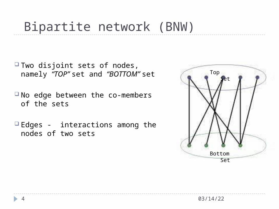
Bipartite network (BNW)
Two disjoint sets of nodes, namely “TOP” set and “BOTTOM” set
No edge between the co-members of the sets
Edges - interactions among the nodes of two sets
04/18/234
Top Set
Bottom Set

BNW growth
One top node is introduced at each time step
Top nodes enter the system with µ edges ( 1≤ µ)
Each top node can bring m new bottom nodes (1≤ m <µ). If m=0, the bottom set is fixed.
Edges are attached randomly or preferentially
04/18/235
04/18/236
Introduction to Bipartite network (BNW) and BNW growth
Why BNWs ? Classes of Growth Models
Sequential attachment growth model (SA) Parallel attachment with replacement growth model (PAWR) parallel attachment without replacement growth model (PAWOR)
One-mode Projection Model verification Conclusions and future works
Contents of the presentation
Many real world examples
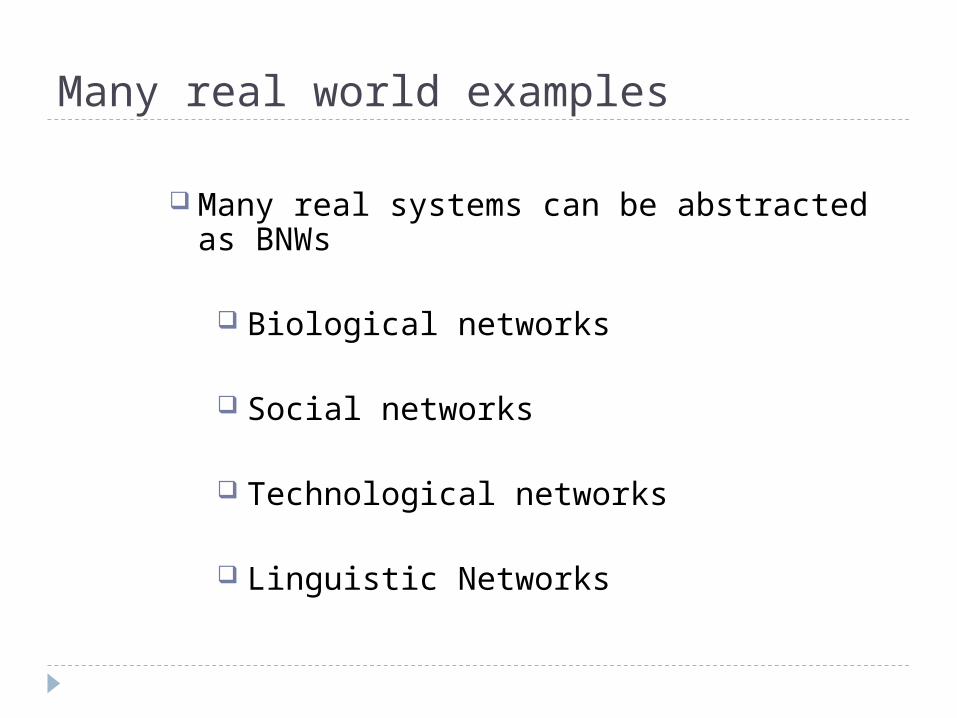
Many real systems can be abstracted as BNWs
Biological networks
Social networks
Technological networks
Linguistic Networks

A regulatory system network
The output data are driven by regulatory signals through a bipartite network
Liao J. C. et.al. PNAS 2003;100:15522-15527
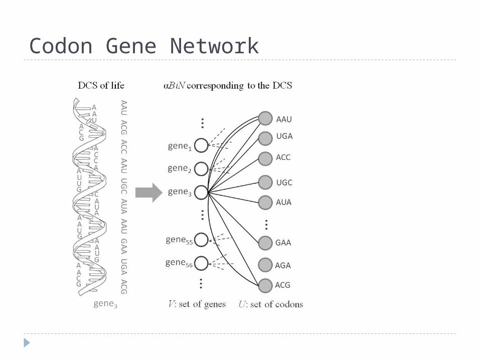
Codon Gene Network

Disease Genome Network
Goh K. et.al. PNAS 2007;104:8685-8690

People Project Network
Bipartite network of people and projects funded by the UK eScience initiatives
The people are circles and the projects are squares.
The color and size of the nodes indicates degree; redder and bigger nodes have more connections than smaller and yellower nodes
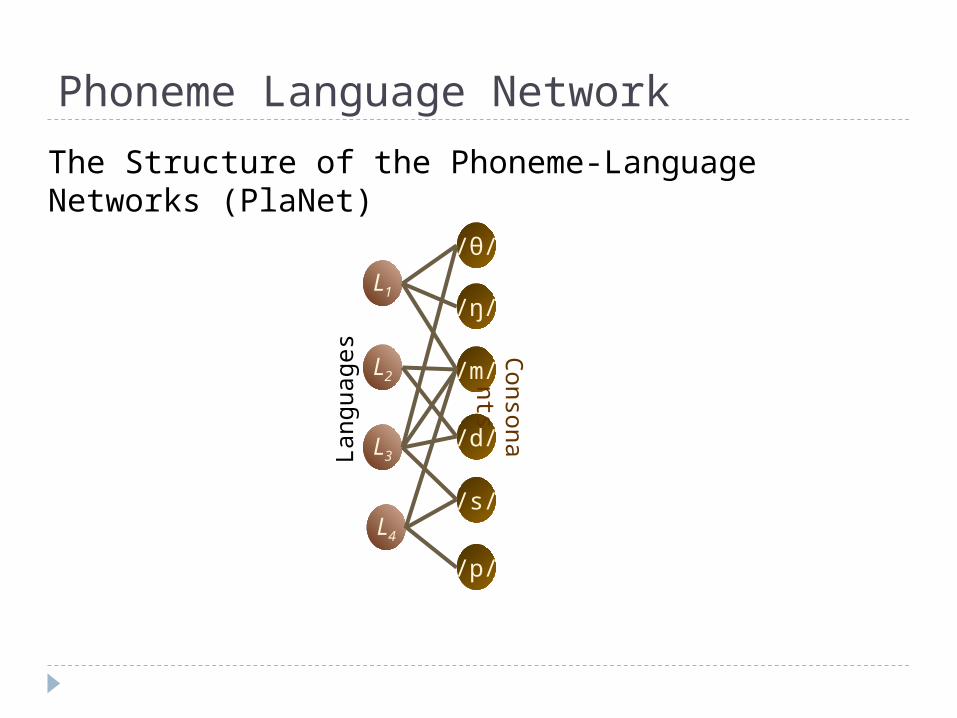
Phoneme Language Network
The Structure of the Phoneme-Language Networks (PlaNet)
L1
L4
L2
L3
/m/
/ŋ/
/p/
/d/
/s/
/θ/
Conso
na
nts
Langu
ages

And many others……. Protein-protein complex network
Movie-actor network
Article-author network
Board-director network
City-people network
Word-sentence network
Bank-company network

04/18/2314
Introduction to Bipartite network (BNW) and BNW growth
Why BNWs ? Classes of Growth Models
Sequential attachment growth model (SA) Parallel attachment with replacement growth model (PAWR) parallel attachment without replacement growth model (PAWOR)
One-mode Projection Model verification Conclusions and future works
Contents of the presentation

Two broad categories
Both partitions grow with time Empirical and analytical studies are available
Ramasco J. J., Dorogovtsev S. N. and Pastor-Satorras R., Phys. Rev. E, 70 (036106) 2004.
Only one partition grows and other remains fixed Couple of empirical studies but no analytical research

Two broad categories
Both partitions grow with time Empirical and analytical studies are available
Ramasco J. J., Dorogovtsev S. N. and Pastor-Satorras R., Phys. Rev. E, 70 (036106) 2004.
Only one partition grows and other remains fixed Couple of empirical studies but no analytical research
with many real examples: Protein protein complex network, Station train network, Phoneme language network etc….

BNW growth with the set of bottom nodes fixed
Fixed number of bottom nodes (N)
One top node is introduced at each time step
Top nodes enter with µ edges
Edges get attached preferentially
04/18/2317
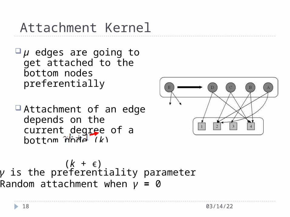
Attachment Kernel
µ edges are going to get attached to the bottom nodes preferentially
Attachment of an edge depends on the current degree of a bottom node (k)
(k + €)
04/18/2318
• γ is the preferentiality parameter• Random attachment when γ = 0
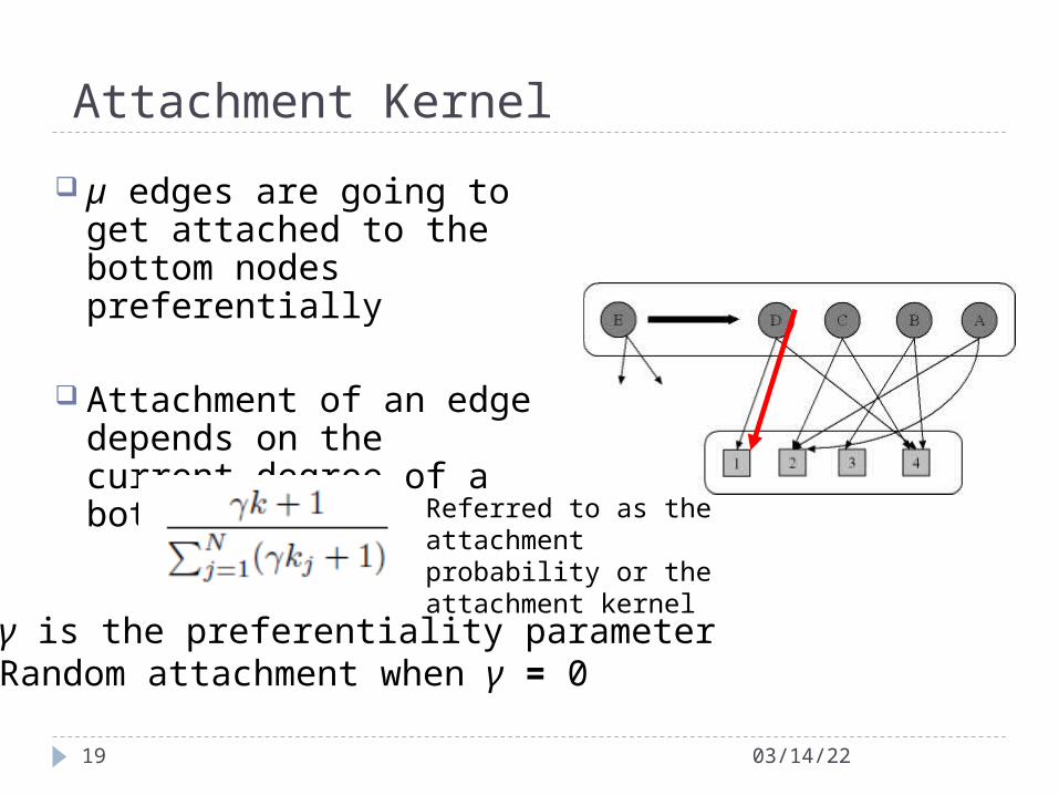
Attachment Kernel
µ edges are going to get attached to the bottom nodes preferentially
Attachment of an edge depends on the current degree of a bottom node (k)
04/18/2319
• γ is the preferentiality parameter• Random attachment when γ = 0
Referred to as the attachment probability or the attachment kernel
Contents of the presentation
04/18/2320
Introduction to Bipartite network (BNW) and BNW growth
Why BNWs ? Classes of Growth Models
Sequential attachment growth model (SA) Parallel attachment with replacement growth model (PAWR) parallel attachment without replacement growth model (PAWOR)
One-mode Projection Model verification Conclusions and future works
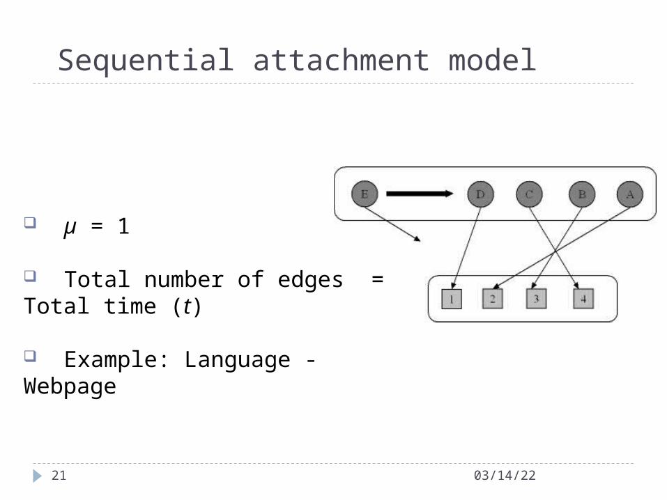
Sequential attachment model
04/18/2321
µ = 1
Total number of edges = Total time (t)
Example: Language - Webpage
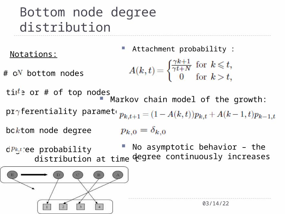
Bottom node degree distribution
04/18/2322
Attachment probability :
Markov chain model of the growth:
No asymptotic behavior – the degree continuously increases
Notations:
- # of bottom nodes
- time or # of top nodes
- preferentiality parameter
- bottom node degree
- degree probability distribution at time t

Bottom node degree distribution
04/18/2323
Attachment probability :
Markov chain model of the growth:
Degree distribution function
Notations:
- # of bottom nodes
- time or # of top nodes
- preferentiality parameter
- bottom node degree
- degree probability distribution at time t
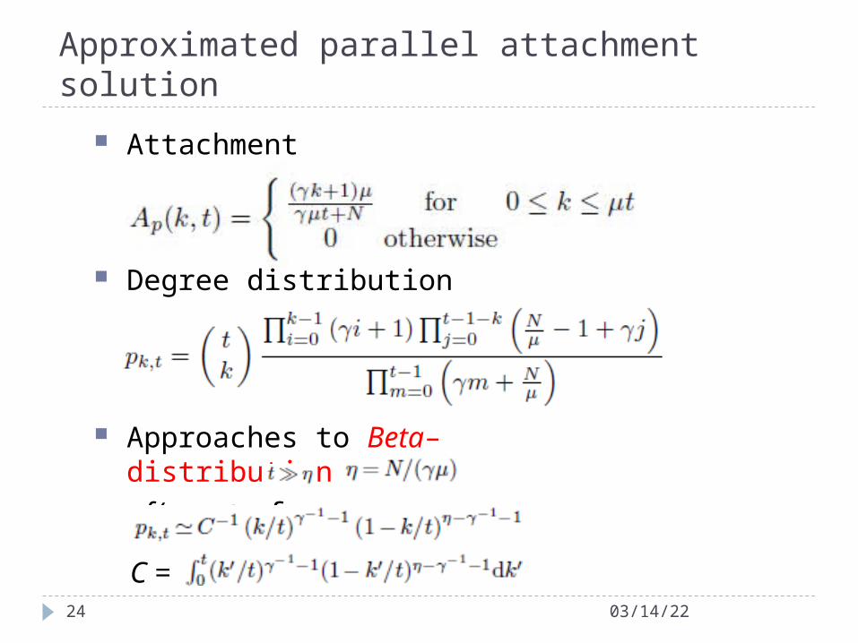
Approximated parallel attachment solution
04/18/2324
Attachment probability :
Degree distribution function
Approaches to Beta– distribution
f(x,α,β) for
C =

Four regimes
04/18/2325
The four possible regimes of degree distributions depending on . (a) , (b) (c) (d)
04/18/2326
Introduction to Bipartite network (BNW) and BNW growth
Why BNWs ? Classes of Growth Models
Sequential attachment growth model (SA) Parallel attachment with replacement growth model (PAWR) parallel attachment without replacement growth model (PAWOR)
One-mode Projection Model verification Conclusions and future works
Contents of the presentation
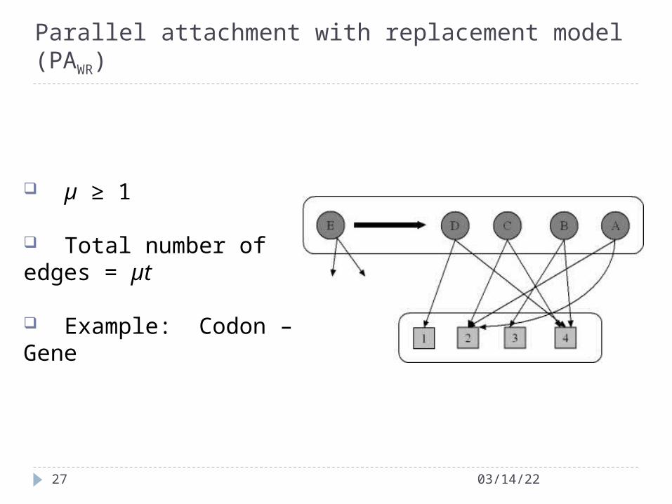
Parallel attachment with replacement model (PAWR)
04/18/2327
µ ≥ 1
Total number of edges = µt
Example: Codon – Gene

04/18/2328
For random attachment, we can derive the attachment probability as
Attachment probability of edges to a bottom nodeof degree k at time t
Exact solution of PAWR

04/18/2329
Introducing preferentiality in the model
For random attachment, we can derive the attachment probability as
Attachment probability of edges to a bottom nodeof degree k at time t
Exact solution of PAWR
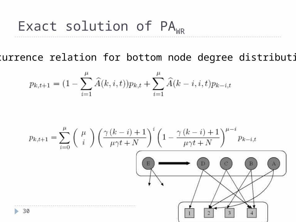
04/18/2330
Recurrence relation for bottom node degree distribution
Exact solution of PAWR

(a) N = 20, t = 250, µ = 40, γ = 1(b) γ = 16
Degree(k)
Pro
babi
lity
of
havi
ng d
egre
e k
Pro
babi
lity
of
havi
ng d
egre
e k
Exactness of exact solution of PAWR
Degree(k)
Solid black curve –> Exact solutionSymbols –> SimulationDashed red curve –> Approximation Approximation fails but exact
solution does well

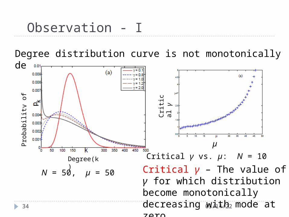
Observations on PAWR
04/18/2332
Degree distribution curve is not monotonically decreasing for γ = 1
Two maxima in bottom node degree distribution plots
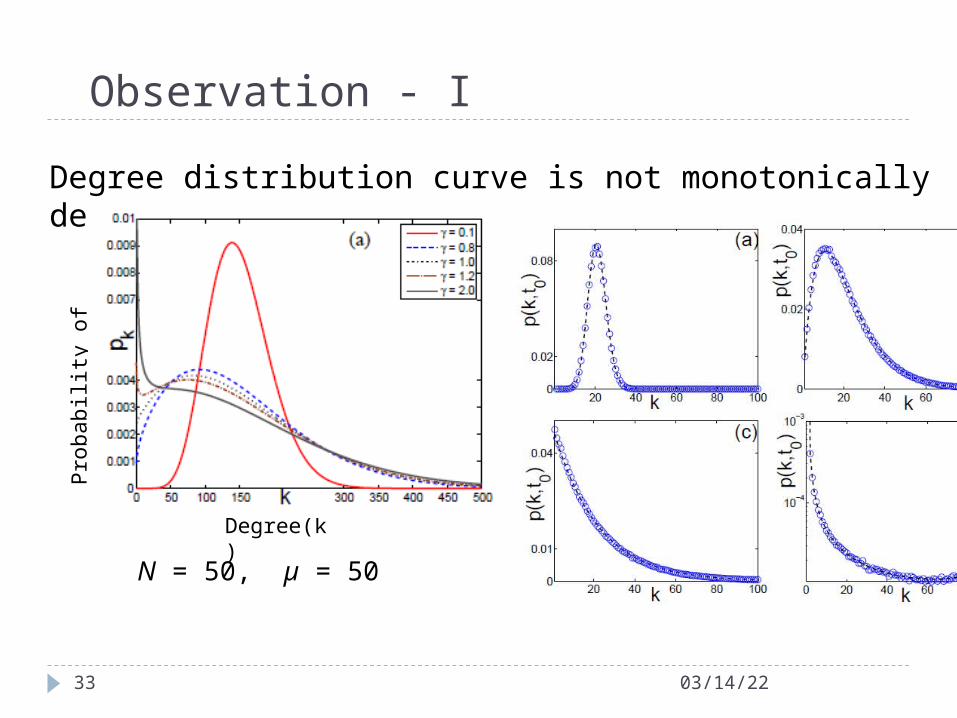
Observation - I
04/18/2333
Degree distribution curve is not monotonically decreasing for γ = 1
Degree(k)
N = 50, µ = 50
Pro
babi
lity
of
havi
ng d
egre
e k
Observation - I
04/18/2334
Degree distribution curve is not monotonically decreasing for γ = 1
N = 50, µ = 50
Degree(k)
Pro
babi
lity
of
havi
ng d
egre
e k
Cri
tica
l γ
µ
Critical γ – The value of γ for which distribution become monotonically decreasing with mode at zero
Critical γ vs. µ: N = 10
04/18/2335
Introduction to Bipartite network (BNW) and BNW growth
Why BNWs ? Classes of Growth Models
Sequential attachment growth model (SA) Parallel attachment with replacement growth model (PAWR) parallel attachment without replacement growth model (PAWOR)
One-mode Projection Model verification Conclusions and future works
Contents of the presentation
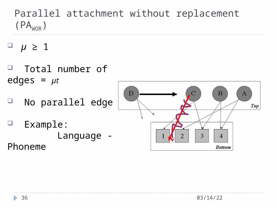
Parallel attachment without replacement (PAWOR)
04/18/2336
µ ≥ 1
Total number of edges = µt
No parallel edge
Example: Language - Phoneme

PAWOR Model - I µ edges connect one by one to µ distinct bottom nodes
After attachment of every edge attachment kernel changes as
Theoretical analysis is almost intractable
04/18/2337
W is the subset of bottom nodes already chosen by the current top node

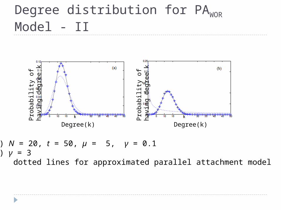
(a) N = 20, t = 50, µ = 5, γ = 0.1(b) γ = 3
Degree(k)
Pro
babi
lity
of
havi
ng d
egre
e k
Degree(k)
Pro
babi
lity
of
havi
ng d
egre
e k
Degree distribution for PAWOR Model - I
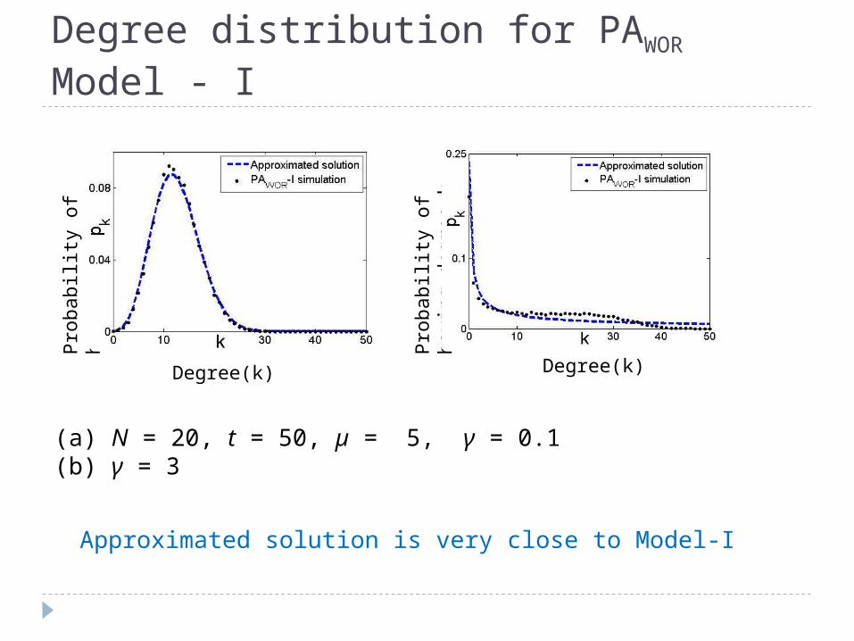
Degree distribution for PAWOR Model - I
(a) N = 20, t = 50, µ = 5, γ = 0.1(b) γ = 3
Degree(k)
Pro
babi
lity
of
havi
ng d
egre
e k
Degree(k)
Pro
babi
lity
of
havi
ng d
egre
e k
Approximated solution is very close to Model-I

PAWOR Model - II
A subset of µ nodes is selected from N bottom nodes preferentially. NCμ sets
Attachment of edges depends on the sum of degrees of member nodes
Each of the selected µ bottom nodes get attached through one edge with the top node
04/18/2340

04/18/2341
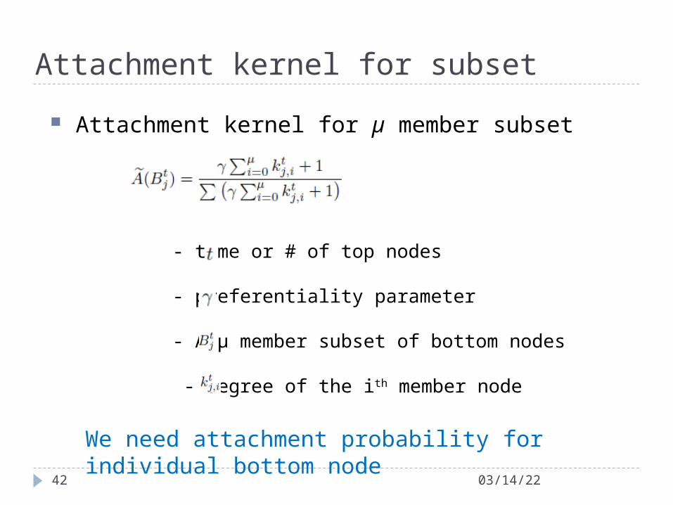
Attachment kernel for µ member subset
- time or # of top nodes
- preferentiality parameter
- A µ member subset of bottom nodes
- degree of the ith member node
Attachment kernel for subset
Attachment kernel for subset
04/18/2342
Attachment kernel for µ member subset
- time or # of top nodes
- preferentiality parameter
- A µ member subset of bottom nodes
- degree of the ith member node
We need attachment probability for individual bottom node

04/18/2343
Any specific bottom node (b) is member of number of subsets
Among those subsets any other bottom node except b has membership in number of subsets
Attachment probability for a bottom node is sum of the attachment probabilities of all container subsets
Sum of degrees of all nodes is
Attachment probability for a single node

Attachment probability for a single node
04/18/2344
Attachment probability for bottom nodes

Bottom node degree distribution
04/18/2345
Markov chain model of the growth:
Degree distribution for PAWOR Model - II
(a) N = 20, t = 50, µ = 5, γ = 0.1(b) γ = 3 dotted lines for approximated parallel attachment model
Degree(k)
Pro
babi
lity
of
havi
ng d
egre
e k
Degree(k)
Pro
babi
lity
of
havi
ng d
egre
e k

Degree distribution for PAWOR Model - II
(a) N = 20, t = 50, µ = 5, γ = 0.1(b) γ = 3 dotted lines for approximated parallel attachment model
Degree(k)
Pro
babi
lity
of
havi
ng d
egre
e k
Degree(k)
Pro
babi
lity
of
havi
ng d
egre
e k
Only skewed binomial distributions are observedExtra randomness in the model
04/18/2348
Introduction to Bipartite network (BNW) and BNW growth
Why BNWs ? Classes of Growth Models
Sequential attachment growth model (SA) Parallel attachment with replacement growth model (PAWR) parallel attachment without replacement growth model (PAWOR)
One-mode Projection Model verification Conclusions and future works
Contents of the presentation

One mode projection of bottom
Goh K. et.al. PNAS 2007;104:8685-8690

Degree of the nodes in One-mode
Easy to calculate if each node v in growing partition enters with exactly (> 1) edges
Consider a node u in the non-growing partition having degree k
u is connected to k nodes in the growing partition and each of these k nodes are in turn connected to -1 other nodes in the non-growing partition
Hence degree q=k(-1)

Bipartite Networks
One-Mode Networks
What if is not fixed??
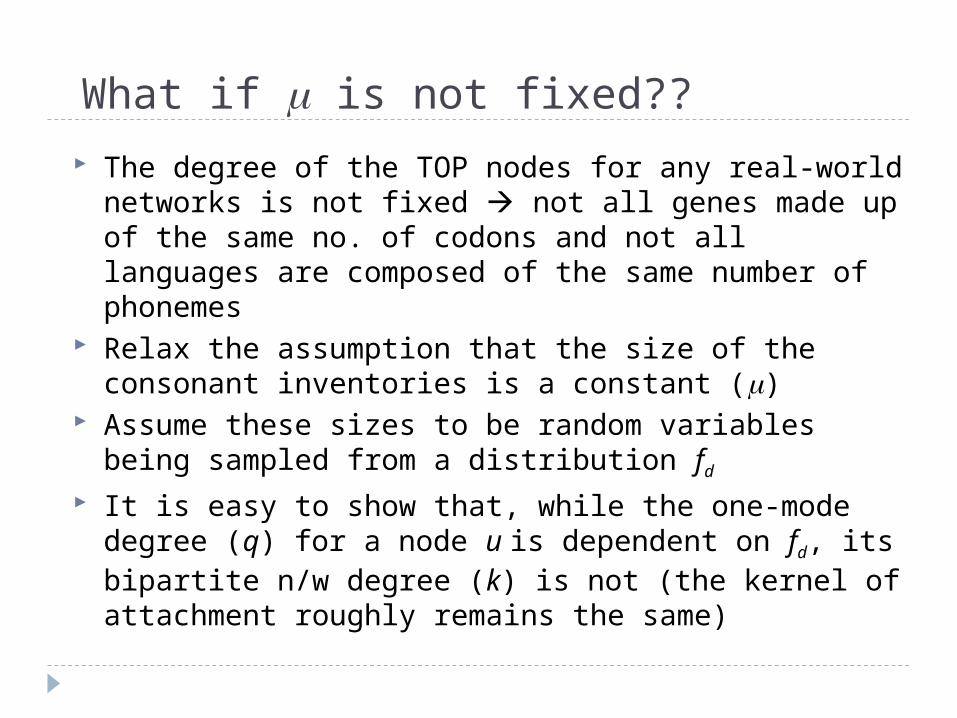
What if is not fixed??
The degree of the TOP nodes for any real-world networks is not fixed not all genes made up of the same no. of codons and not all languages are composed of the same number of phonemes
Relax the assumption that the size of the consonant inventories is a constant ()
Assume these sizes to be random variables being sampled from a distribution fd
It is easy to show that, while the one-mode degree (q) for a node u is dependent on fd, its bipartite n/w degree (k) is not (the kernel of attachment roughly remains the same)

Analysis of Degree Distribution Assume that the k nodes in TOP partition to which a
BOTTOM node u is connected to have degrees
The probability that u is connected to a node of degree d1 is d1fd1
, d2 is d2fd2, …, dk is dkfdk
The normalized probability that u is connected to nodes of degree d1, d2, … dk is

Analysis of Degree Distribution
Fk(q): The probability that node u having degree k in the bipartite network ends up as a node having degree q in the one-mode projection
Now add up these probabilities for all values of k weighted by the probability of finding a node of degree k in the bipartite network
Analysis of Degree Distribution
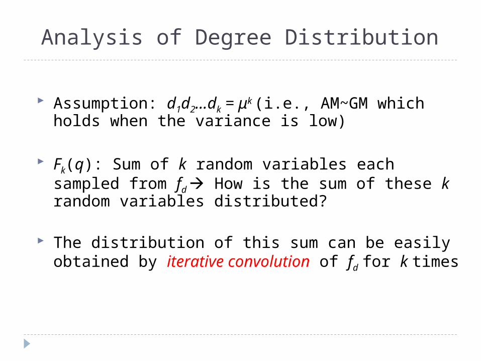
Assumption: d1d2…dk = μk (i.e., AM~GM which holds when the variance is low)
Fk(q): Sum of k random variables each sampled from fd How is the sum of these k random variables distributed?
The distribution of this sum can be easily obtained by iterative convolution of fd for k times
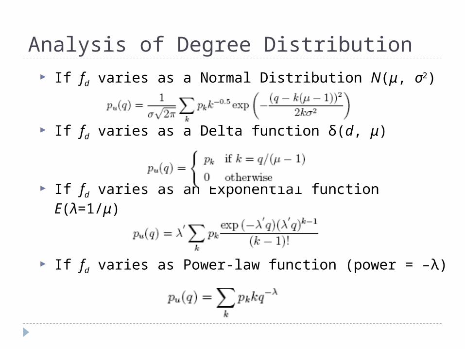
Analysis of Degree Distribution
If fd varies as a Normal Distribution N(μ, σ2)
If fd varies as a Delta function δ(d, μ)
If fd varies as an Exponential function E(λ=1/μ)
If fd varies as Power-law function (power = –λ)

Results of the Analysis
N = 1000, t = 1000,γ= 2,μ=22
Bipartite Networks One-Mode
Networks

04/18/2358
Introduction to Bipartite network (BNW) and BNW growth
Why BNWs ? Classes of Growth Models
Sequential attachment growth model Parallel attachment with replacement growth model parallel attachment without replacement growth model
One-mode Projection Model verification Conclusions and future works
Contents of the presentation
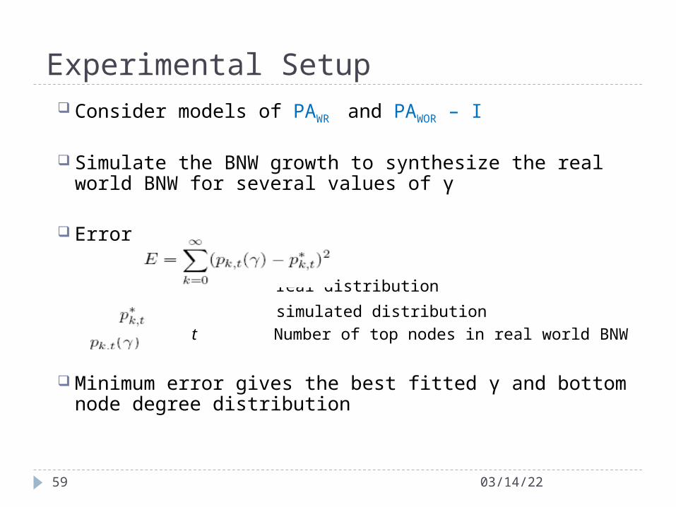
Experimental Setup Consider models of PAWR and PAWOR – I
Simulate the BNW growth to synthesize the real world BNW for several values of γ
Error
real distribution
simulated distribution
t Number of top nodes in real world BNW
Minimum error gives the best fitted γ and bottom node degree distribution
04/18/2359

Phoneme-Language Network
Top – Language
Fixed bottom - Phoneme
N – 541 (phonemes)
t – 317 (language)
µ – 22
04/18/2360
Data - UCLA Phonological Segment Inventory Database (UPSID)
EWOR = 0.113062928EWR = 0.109411487
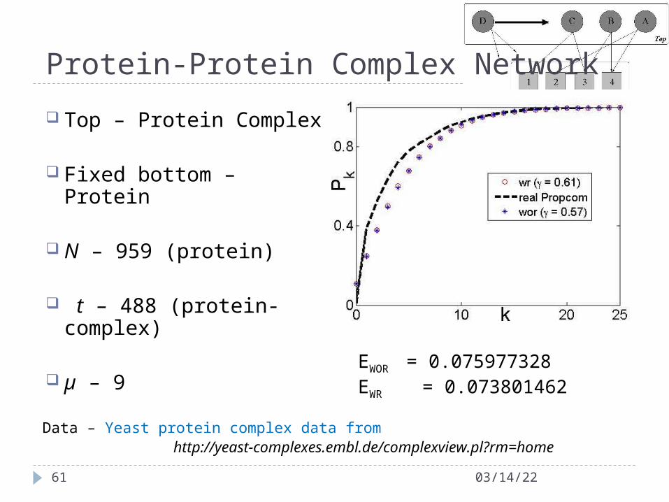
Protein-Protein Complex Network
04/18/2361
Top – Protein Complex
Fixed bottom – Protein
N – 959 (protein)
t – 488 (protein-complex)
µ – 9
Data – Yeast protein complex data from http://yeast-complexes.embl.de/complexview.pl?rm=home
EWOR = 0.075977328EWR = 0.073801462

Station-Train Network
04/18/2362
Top – Train
Fixed bottom – Station
N – 2764 (Station)
t – 1377 (Train)
µ – 26
Data – Indian Railway data from http://www.indianrail.gov.in
EWOR = 0.034344613EWR = 0.034138636

04/18/2363
Introduction to Bipartite network (BNW) and BNW growth
Why BNWs ? Classes of Growth Models
Sequential attachment growth model Parallel attachment with replacement growth model parallel attachment without replacement growth model
One-mode Projection Model verification Conclusions and future works
Contents of the presentation
The dynamics of BNWs where one of the partitions is fixed and finite over time is different from those where both the partitions grow unboundedly. While the former approaches a β–distribution, the latter results in a
power-law in the asymptotic limits Many real-world systems can be modeled as BNWs with one
partition fixed (e.g., Phoneme-Language N/w, Protein-Protein Complex N/w, Train-Station N/w)
The growth dynamics of these n/ws can be suitably explained through simple preferential attachment based models coupled with a tunable parameter controlling the amount of preferentiality/randomness of the growth process.
The degree distribution of one-mode projection onto the BOTTOM nodes depends on how the TOP node degrees are distributed in the BNW
Conclusions and Future works

Conclusions and Future works
Future works include
Deriving closed form solutions for PAWR and PAWOR models. Understanding their (non)equivalence.
Exploring the dynamics of the models for non-linear kernels, i.e., the attachment probability is proportional to kα where α < 1 refers to sub-linear kernels and α > 1 to super-linear kernels
Analytically deriving other structural properties of the one-mode like clustering coefficient, assortativity etc.

Collaborators
Animesh Mukherjee, Abyayananda Maity – IIT Kharagpur
Monojit Choudhury – Microsoft Research India
Fernando Peruani – CEA, Sacalay, France
Andreas Deutsch, Lutz Brusch – TU Dresden, Germany
04/18/2366

Contributing literature
1. F. Peruani, M. Choudhury, A. Mukherjee, and N. Ganguly. Emergence of a non-scaling degree distribution in bipartite networks: A numerical and analytical study. Europhys. Lett., 79:28001, 2007.
2. M. Choudhury, N. Ganguly, A. Maiti, A. Mukherjee, L. Brusch, A. Deutsch, and F. Peruani. Modeling discrete combinatorial systems as alphabetic bipartite networks: Theory and applications. (communicated to “Physical Review E”).
3. A. Mukherjee, M. Choudhury and N. Ganguly. Analyzing the Degree Distribution of the One-mode Projection of Alphabetic Bipartite Networks (α-- BiNs) (communicated to “Europhys. Lett.”).
04/18/2367

Dynamics On and Of Complex Networks
Applications to Biology, Computer Science, and the Social SciencesSeries: Modeling and Simulation in Science, Engineering and Technology Ganguly, Niloy; Deutsch, Andreas; Mukherjee, Animesh (Eds.) A Birkhäuser book
Workshop – 23rd September, Warwick

Dziękuję
04/18/2370

Pro
babi
lity
of
havi
ng d
egre
e k
Observation - I
04/18/2371
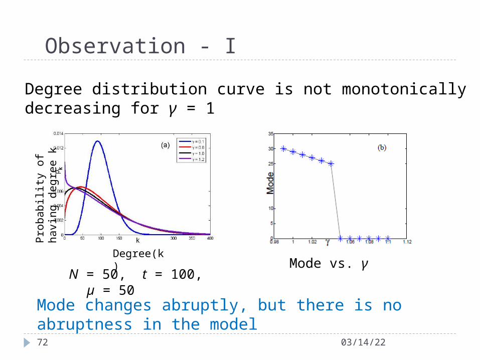
Degree distribution curve is not monotonically decreasing for γ = 1
N = 50, t = 100, µ = 50
Degree(k) Mode vs. γ
Observation - I
04/18/2372
Degree distribution curve is not monotonically decreasing for γ = 1
N = 50, t = 100, µ = 50
Degree(k)
Pro
babi
lity
of
havi
ng d
egre
e k
Mode vs. γ
Mode changes abruptly, but there is no abruptness in the model
Observation – I cont.
04/18/2373
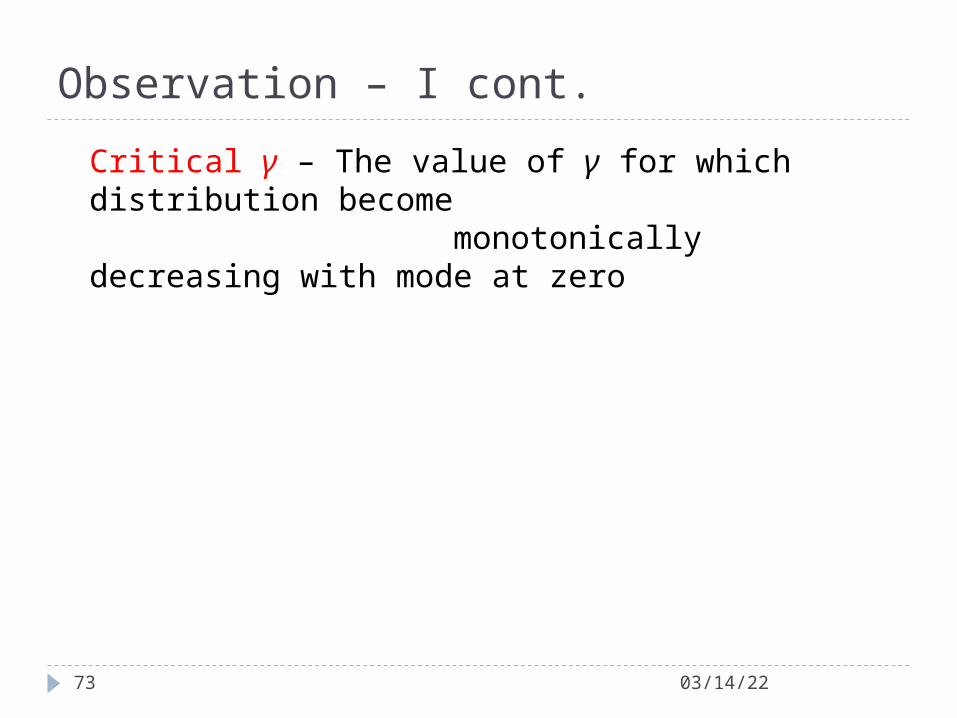
Critical γ – The value of γ for which distribution become monotonically decreasing with mode at zero

Observation – I cont.
04/18/2374
Critical γ – The value of γ for which distribution become monotonically decreasing with mode at zero
(a) Critical γ vs. µ: N = 10, t = 50
Cri
tica
l γ
µ

Observation – I cont.
04/18/2375
Critical γ – The value of γ for which distribution become monotonically decreasing with mode at zero
(a) Critical γ vs. µ: N = 10, t = 50
Cri
tica
l γ
µ
Critical γ is directly proportional to µ in exponential manner

Observation – I cont.
04/18/2376
Critical γ – The value of γ for which distribution become monotonically decreasing with mode at zero
(a) Critical γ vs. µ: N = 10, t = 50(b) Mode vs. µ: γ = 1.2, at µ = 16 mode becomes zero
Cri
tica
l γ
µ
Critical γ is directly proportional to µ in exponential manner
µ

Observation – I cont.
04/18/2377
(a) Critical γ vs. time: N = 10, µ = 5
Time (t)
Cri
tica
l γ
04/18/2378
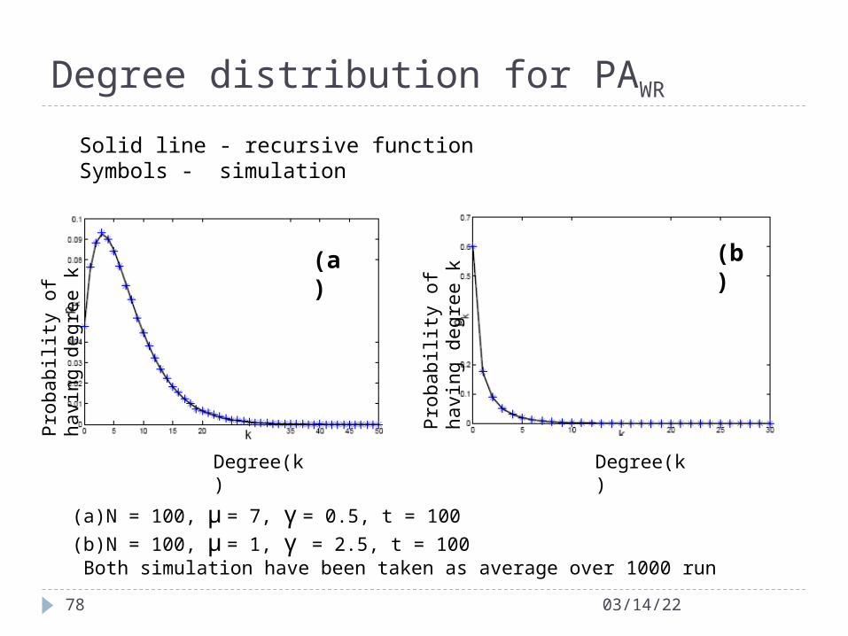
(a) N = 100, µ = 7, γ = 0.5, t = 100
(b) N = 100, µ = 1, γ = 2.5, t = 100 Both simulation have been taken as average over 1000 run
(a)
(b)
Solid line - recursive function Symbols - simulation
Degree(k)
Pro
babi
lity
of
havi
ng d
egre
e k
Degree distribution for PAWR
Degree(k)
Pro
babi
lity
of
havi
ng d
egre
e k
Observation – I cont.
04/18/2379
(a) Critical γ vs. time: N = 10, µ = 5
Time (t)
Cri
tica
l γ
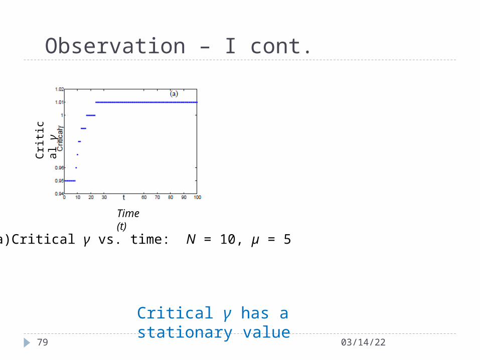
Critical γ has a stationary value
Observation – I cont.
04/18/2380
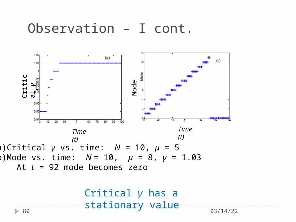
(a) Critical γ vs. time: N = 10, µ = 5(b) Mode vs. time: N = 10, µ = 8, γ = 1.03 At t = 92 mode becomes zero
Time (t)
Cri
tica
l γ
Critical γ has a stationary value
Time (t)M
ode

Observation – I cont.
04/18/2381
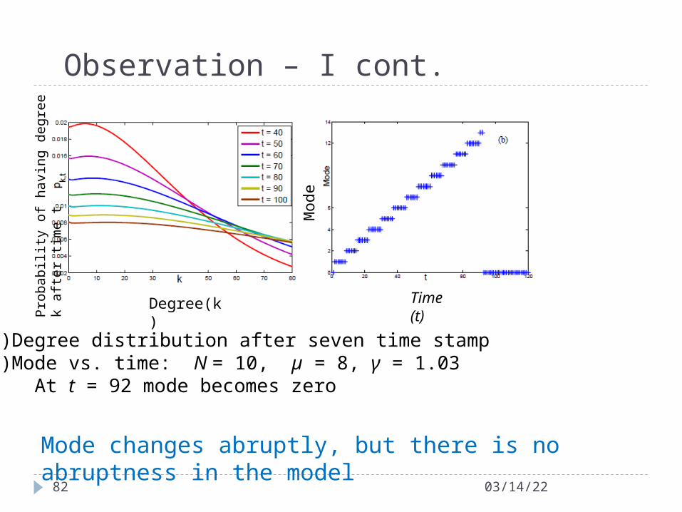
(a) Degree distribution after seven time stamp(b) Mode vs. time: N = 10, µ = 8, γ = 1.03 At t = 92 mode becomes zero
Critical γ has a stationary value
Time (t)M
ode
Degree(k)
Pro
babi
lity
of
havi
ng d
egre
e k
afte
r ti
me
t
Observation – I cont.
04/18/2382
(a) Degree distribution after seven time stamp(b) Mode vs. time: N = 10, µ = 8, γ = 1.03 At t = 92 mode becomes zero
Time (t)M
ode
Degree(k)
Pro
babi
lity
of
havi
ng d
egre
e k
afte
r ti
me
t
Mode changes abruptly, but there is no abruptness in the model

Observation - II
04/18/2383
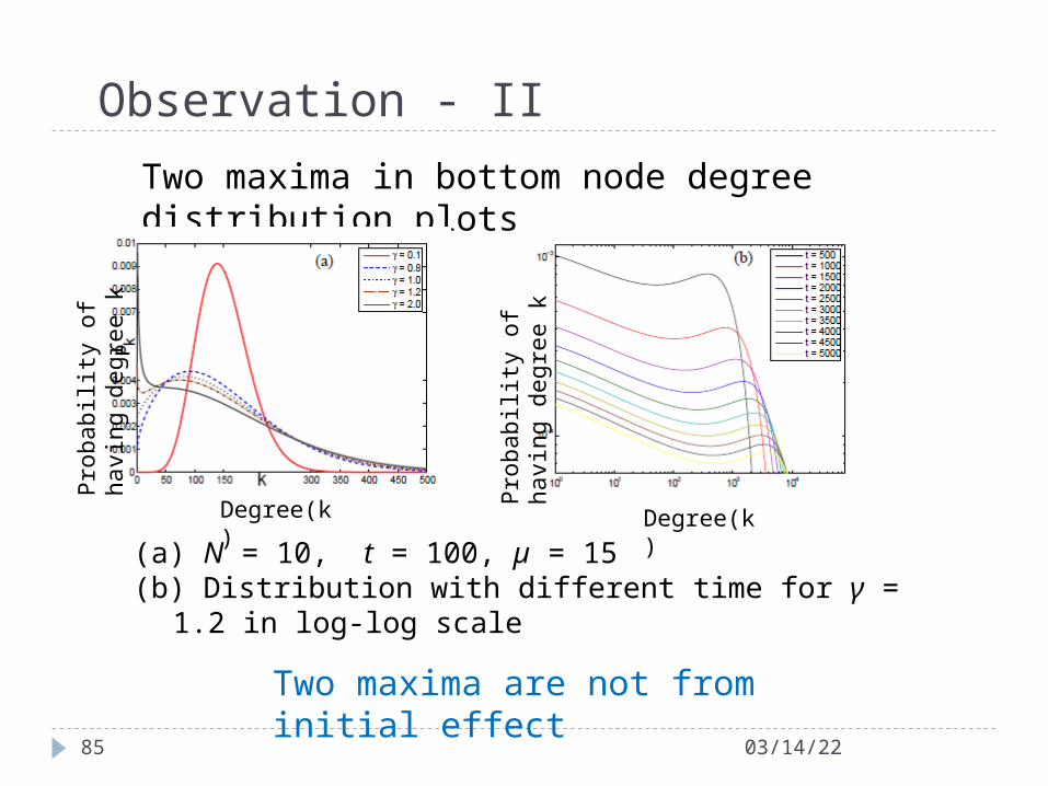
(a) N = 10, t = 100, µ = 15
Two maxima in bottom node degree distribution plots
Degree(k)
Pro
babi
lity
of
havi
ng d
egre
e k

Observation - II
04/18/2384
(a) N = 10, t = 100, µ = 15(b) Distribution with different time for γ = 1.2 in log-log scale
Two maxima in bottom node degree distribution plots
Degree(k)
Pro
babi
lity
of
havi
ng d
egre
e k
Degree(k)P
roba
bili
ty o
f ha
ving
deg
ree
k
Observation - II
04/18/2385
(a) N = 10, t = 100, µ = 15(b) Distribution with different time for γ = 1.2 in log-log scale
Two maxima in bottom node degree distribution plots
Degree(k)
Pro
babi
lity
of
havi
ng d
egre
e k
Degree(k)P
roba
bili
ty o
f ha
ving
deg
ree
k
Two maxima are not from initial effect

Observation – II cont.
04/18/2386
(a) First min and second max degree over time for N = 10, µ = 15, γ = 1.2
Time(t)
Min
\ M
ax d
egre
e
Observation – II cont.
04/18/2387
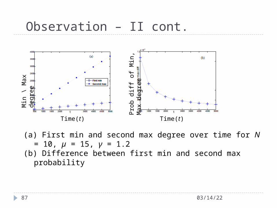
(a) First min and second max degree over time for N = 10, µ = 15, γ = 1.2(b) Difference between first min and second max probability
Time(t)
Min
\ M
ax d
egre
e
Pro
b di
ff o
f M
in, M
ax d
egre
e
Time(t)

Observation – II cont.
04/18/2388
(a) First min and second max degree over time for N = 10, µ = 15, γ = 1.2(b) Difference between first min and second max probability
Time(t)
Min
\ M
ax d
egre
e
Pro
b di
ff o
f M
in, M
ax d
egre
e
Time(t)
Probability difference may get a non-zero value asymptotically