gravitational axial perturbations and quasinormal modes of ... · gravitational axial perturbations...
TRANSCRIPT

Prepared for submission to JCAP
Gravitational axial perturbationsand quasinormal modes of loopquantum black holes
M.B.Cruz,a C.A.S.Silva, b,1 F.A.Britoc
aDepartamento de Física, Universidade Federal da Paraíba, 58051-970, João Pessoa, Paraíba,Brazil.bInstituto Federal de Educação Ciência e Tecnologia da Paraíba (IFPB),Campus Campina Grande - Rua Tranquilino Coelho Lemos, 671, Jardim Dinamérica I,Campina Grande, Paraíba, Brazil.cDepartamento de Física, Universidade Federal de Campina Grande Caixa Postal 10071,58429-900 Campina Grande, Paraíba, Brazil.
E-mail: [email protected], [email protected],[email protected]
Abstract. Loop Quantum Gravity (LQG) is a theory that proposes a way to model thebehavior of the spacetime in situations where its atomic characteristic arises. Among thesesituations, the spacetime behavior near the Big Bang or black hole’s singularity. The detectionof gravitational waves, on the other hand, has opened the way to new perspectives in theinvestigation of the spacetime structure. In this work, by the use of a WKBmethod introducedby Schutz and Will [1], and after improved by Iyer and Will [2], we study the gravitationalwave spectrum emitted by loop quantum black holes, which correspond to a quantized versionof Schwarzschild spacetime by LQG techniques. From the results obtained, loop quantumblack holes have been shown stable under axial gravitational perturbations.
1Corresponding author.
arX
iv:1
511.
0826
3v2
[gr
-qc]
1 A
ug 2
017
Contents
1 Introduction 1
2 Loop quantum black holes 2
3 Regge-Wheeler formalism for LQBH 5
4 Quasinormal modes from LQBHs 8
5 Conclusions and perspectives 12
1 Introduction
One of most exiting predictions of general relativity is the existence of black holes, objects fromwhich no physical bodies or signals can get loose of their drag due to its strong gravitationalfield. Going far beyond astrophysics, black holes appear as objects that may help us toclarify one of the most intriguing bone of contention in the current days, the quantum natureof gravity. It is because, in the presence of a black hole’s strong gravitational field, quantumfeatures of spacetime must be manifested [3–9].
Loop quantum gravity, on the other hand, is a theory that has given ascent to modelsthat provide a portrait of the quantum features of spacetime unveiled by a black hole. Inparticular, in the context of this theory, a black hole metric known as Loop Quantum BlackHole (LQBH), or self-dual black hole, has been proposed [10, 11]. This solution correspondsto a quantum corrected Schwarzschild solution and possess the interesting property of self-duality. From this property, the black hole singularity is removed and replaced by anotherasymptotically flat region, which is an expected effect in a quantum gravity regime. Moreover,LQBHs have been pointed as a possible candidate for dark matter [11, 12] and as the buildingblocks of a holographic version of loop quantum cosmology [13].
In order to move black holes from a simple mathematical solution of the gravitationalequations to objects whose existence in nature is possible, a key point consists in to investigateblack hole’s stability under perturbations. It is due to the fact that an isolated black holewould never been found in nature. In fact, complex distributions of matter such as accretiondisks, galactic nuclei, strong magnetic fields, other stars, etc are always present around blackholes, which in turn actively interact with their surroundings. Even if all macroscopic objectsand fields in space have been removed, a black hole will interact with the vacuum around it,creating pairs of particles and evaporating due to Hawking phenomena. Besides, in the firstmoments after its formation, a black hole is in a perturbed state due to gravitational collapseof matter. In this way, a real black hole will be always in a perturbed state.
Black hole’s response to a perturbation occurs by emitting gravitational waves whoseevolution corresponds, firstly, to a relatively short period of initial outburst of radiationfollowed by a phase where the black hole get going to vibrating into exponentially decayingoscillations, “quasinormal modes”, whose frequencies and decay times depend only on theintrinsic characteristics of the black hole itself, being indifferent to the details of the collapse.Finally, at a very large time, the quasinormal modes are slapped down by power-law orexponential late-time tails.
– 1 –

The issue of black hole stability under perturbations was firstly addressed by Regge-Wheeler [14] and Zerilli [15], which based on black hole perturbation theory, have demon-strated the stability of the Schwarzschild metric. The methods used are familiar from quantummechanics: perturbations caused by an external (eg., gravitational or electromagnetic) fieldare taken into account as waves scattering off the respective potential. It is due to the factthat the formalism provided by Regge-Wheller and Zerilli removes the angular dependence inthe perturbation variables by the use of a tensorial generalization of the spherical harmonicswhich makes possible to translate the solution of the perturbed Einstein equations in theform of a Schrodinger-like wave equation treatment. Posteriorly, the Regge-Wheeler/Zerilliformalism was extended to the charged [16–18] and rotating [19, 20] black hole scenarios.A full description of the black hole perturbation framework can be found in the text byChandrasekhar [21].
The most valuable phase in the evolution of black hole perturbations is given by itsquasinormal modes which can give us information not only about the black hole stability, butalso, as emphasized by Berti in [22], "‘how much stable it is"’. In other words, quasinormalmodes tell us which timescale a black hole radiate away its matter contend after formation.By the way, in this context the prefix "‘quasi” means that the black hole consists in anopen system that loses energy due to the emission of gravitational waves. The issue of blackhole quasinormal modes is interesting not only by the investigation of black hole stabilitybut also because gravitational waves have been pointed as a possible experimental way tomake contact with black holes and, in this way, with the quantum spacetime characteristicsrevealed by them. Indeed, recent results from LIGO, which has detected a gravitationalsignal from black holes [23–26] have open the floodgates for a large range of possibilities ingravitational physics in the same way that the discovery of infrared radiation by WilliamHershel in the "‘1800’s"’ opened the possibility of the investigation and application of theelectromagnetic spectrum beyond to the visible. It can yet be reinforced by others resultsfrom others gravitational antennas such as LISA VIRGO, and others. In a timely way, thequasinormal fundamental model constitutes the predominating contribution to such signals.
In this work, we shall address the gravitational wave production by LQBHs. Quasinormalfrequencies for such black holes have been addressed for the scalar perturbations case in[27, 28]. However, in a more realistic scenario, gravitational perturbations must be included.Investigation on the quasinormal modes spectrum in the context of LQBHs may reveal someadvantages front others scenarios under the experimental point of view since the quantumcorrections present in this scenario depend on the Barbero-Immirzi parameter [29], which ashas been pointed in [30], does not suffers with the problem of mass suppression as occurs withthe parameters of other quantum gravity theories like superstring theory or noncommutativetheory.
The article is organized as follows: in section (2), we revise the LQBH’s theory; insection (3), we calculate the Regge-Wheeler equation for LQBHs; in section (4), we calculatethe quasinormal modes of the LQBHs. Section (5) is devoted to conclusions and remarks.Through out this paper, we have used ~ = c = G = 1.
2 Loop quantum black holes
Some efforts in order to find out black hole solutions in LQG have been done by severalauthors [10, 31–40]. In this section, we shall analyze a particular solution, called self-dual that
– 2 –
appeared at the primary time from a simplified model of LQG consisting in symmetry reducedmodels corresponding to homogeneous spacetimes (see [10] and the references therein).
In this way, the LQBH framework which we shall work here is delineated by a quantumgravitationally corrected Schwarzschild metric, written as
ds2 = −G(r)dt2 + F−1(r)dr2 +H(r)dΩ2 (2.1)
with
dΩ2 = dθ2 + sin2 θdφ2 , (2.2)
where, in the equation (2.1), the metric functions are given by
G(r) =(r − r+)(r − r−)(r + r∗)
2
r4 + a20, F (r) =
(r − r+)(r − r−)r4
(r + r∗)2(r4 + a20), (2.3)
and
H(r) = r2 +a20r2
, (2.4)
where
r+ = 2m ; r− = 2mP 2 .
In this situation, we have got the presence of two horizons - an event horizon localized at r+and a Cauchy horizon localized at r−.
Furthermore, we have that
r∗ =√r+r− = 2mP . (2.5)
In the definition above, P is the polymeric function given by
P =
√1 + ε2 − 1√1 + ε2 + 1
; (2.6)
and
a0 =Amin
8π. (2.7)
where Amin is the minimal value of area in LQG.In the metric (2.1), r is only asymptotically the same old radial coordinate since gθθ is
not simply r2. A more physical radial coordinate is obtained from the shape of the functionH(r) within the metric (2.4)
R =
√r2 +
a20r2
(2.8)
in the sense that it measures the right circumferential distance.Moreover, the parameter m within the solution is related to the ADM mass M by
– 3 –
M = m(1 + P )2 . (2.9)
The equation (2.8) reveals vital aspects of the LQBH’s internal structure. From thisexpression, we have got that, as r decreases from ∞ to 0, R initially decreases from ∞ to√
2a0 at r =√a0 so will increase once more to ∞. The value of R associated with the event
horizon is given by
REH =√H(r+) =
√(2m)2 +
( a02m
)2. (2.10)
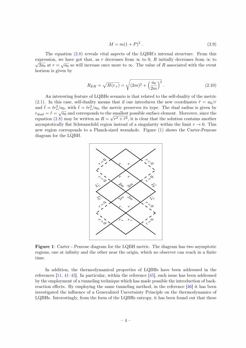
An interesting feature of LQBHs scenario is that related to the self-duality of the metric(2.1). In this case, self-duality means that if one introduces the new coordinates r = a0/rand t = tr2∗/a0, with t = tr2∗/a0, the metric preserves its type. The dual radius is given byrdual = r =
√a0 and corresponds to the smallest possible surface element. Moreover, since the
equation (2.8) may be written as R =√r2 + r2, it is clear that the solution contains another
asymptotically flat Schwazschild region instead of a singularity within the limit r → 0. Thisnew region corresponds to a Planck-sized wormhole. Figure (1) shows the Carter-Penrosediagram for the LQBH.
Figure 1: Carter - Penrose diagram for the LQBH metric. The diagram has two asymptoticregions, one at infinity and the other near the origin, which no observer can reach in a finitetime.
In addition, the thermodynamical properties of LQBHs have been addressed in thereferences [11, 41–45]. In particular, within the reference [45], such issue has been addressedby the employment of a tunneling technique which has made possible the introduction of back-reaction effects. By employing the same tunneling method, in the reference [46] it has beeninvestigated the influence of a Generalized Uncertainty Principle on the thermodynamics ofLQBHs. Interestingly, from the form of the LQBHs entropy, it has been found out that these
– 4 –
objects could be the main constituents of a holographic version of loop quantum cosmology[13].
3 Regge-Wheeler formalism for LQBH
In this section, we shall use a method due to Regge and Wheeler to investigate black hole’saxial gravitational perturbations [14]. In this way, we have that, if small perturbations areintroduced, the resulting spacetime metric can be written as gµν = gµν + hµν , where gµν isthe background metric and hµν is the spacetime perturbation. Moreover, the perturbationsare much smaller than the background. By placing our attention on the perturbation hµν , wehave that, due to spherical symmetry, it can be written in two parts, where one depends onthe angular coordinates through the spherical harmonics and the other one depends on thecoordinates r e t. In addition, hµν can be written as a sum of a polar and an axial component.
In this context, we can find out, in particular, that the axial component of the gravita-tional perturbation of the metric (2.1), can be written, under the Regge-Wheeler gauge, as[47]:
haxialµν =
0 0 0 h0(t, r)0 0 0 h1(t, r)0 0 0 0
h0(t, r) h1(t, r) 0 0
sin θ∂θPl(cos θ)eimφ , (3.1)
which applied in the perturbed field equation
δRµν = δΓαµα;ν − δΓαµν;α = 0, (3.2)
give us the following coupled equations:
δRθφ =1
2
[−G−1∂h0
∂t+ F
∂h1∂r
+1
2F ′h1 +
1
2
G′
GFh1)
]×
cos θ∂Pl(cos θ)
∂θ
− sin θ∂2Pl(cos θ)
∂θ2
= 0, (3.3)
δRrφ =1
2
[G−1
(∂2h0∂t∂r
− H ′
H
∂h0∂t
)+
(− l(l + 1)
Hh1 −G−1
∂2h1∂t2
+1
2F ′H ′
Hh1
+FH ′′
Hh1 +
1
2
G′
GFH ′
Hh1
)]×
sin θ∂l(cos θ)
∂θ
= 0 . (3.4)
In order to handle the equations above, we can observe that values of multipole indicesfor which l < s, are not related to dynamical modes, corresponding to conserved quantities.In this way, we shall consider only the nontrivial radiative multipoles with l ≥ s. On theother hand, a gravitational perturbation corresponding to l = 0 will be related to a black holemass change, and a perturbation corresponding to l = 1 will be related to a displacement aswell as to a change on the black hole angular momentum. The most interesting multipoleindices values are those that correspond to the cases where the wave can propagate during a
– 5 –
time interval large enough to be detected. In this way, only the l ≥ 2 cases are relevant [48].Since, for l ≥ 2, we have Pl≥2 6= 0, we obtain the following radial equations
−G−1∂h0∂t
+ F∂h1∂r
+1
2F ′h1 +
1
2
G′
GFh1 = 0, (3.5)
−∂2h0∂t∂r
+∂2h1∂t2
+H ′
H
∂h0∂t
+
[G
Hl(l + 1)− 1
2GF ′
H ′
H− GFH ′′
H− 1
2
G′FH ′
H
]h1 = 0 . (3.6)
Moreover, from the equation (3.5), we have that
∂h0∂t
= (GF )1/2
(GF )1/2∂h1∂r
+1
2(GF )−1/2GF ′h1 +
1
2(GF )−1/2G′Fh1
= (GF )1/2
∂Q(t, r)
∂r=∂Q(t, r)
∂x, (3.7)
where the function Q(t, r) is defined as
Q(t, r) ≡ (GF )1/2h1(t, r), (3.8)
and the tortoise coordinate x is given by the relation:
∂r
∂x= (GF )1/2 . (3.9)
By integrating the equation above, we obtain
x = r − a20rr−r+
+a20(r− + r+)
r2−r2+
log(r) +(a20 + r4−)
r2−(r− − r+)log(r − r−)
+(a20 + r4+)
r2+(r+ − r−)log(r − r+). (3.10)
Now, if we substitute the equations (3.8) and (3.9) in (3.6) , we obtain:
− d
dr
dQ
dx+ (GF )−1/2
d2Q
dt2+H ′
H
dQ
dx+
[G
Hl(l + 1)− 1
2GF ′
H ′
H−GF H
′′
H
−1
2G′F
H ′
H
](GF )−1/2Q = 0 , (3.11)
which, by using the definition
ψ(t, x(r)) ≡ Q(t, r)
H1/2, (3.12)
can be written as
– 6 –
− d
dr
d
dx(H1/2Ψ) +
(GF
H
)−1/2 d2Ψdt2
+H ′
H
d
dx(H1/2Ψ) +
[G
Hl(l + 1)− 1
2GF ′
H ′
H
−GF H′′
H− 1
2G′F
H ′
H
](GF
H
)−1/2Ψ = 0 . (3.13)
The equation above can be rewritten as a Schrodinger-type equation which reads:
−d2Ψ
dx2+d2Ψ
dt2+ Veff (r(x))Ψ = 0, (3.14)
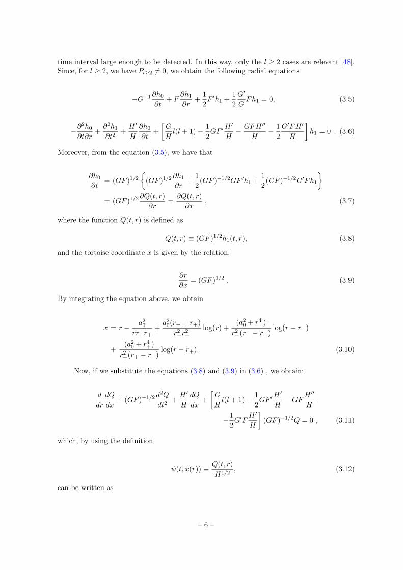
where the effective potential is given by
Veff (r(x)) =r2(r − r−)(r − r+)
(r4 + a20)4
[6r2∗ − 3(r+ + r−) + l(l + 1)(r + r∗)
2]r8
+ 30r4a20[r(r+ + r− − r)− r2∗] + 2r4a20l(l + 1)(r + r∗)2
+ 3ra40[2r − (r+ − r−)] + a40(r + r∗)2l(l + 1)
. (3.15)
The LQBH potential behavior in relation to the r and x coordinates are, respectively, depictedin the figure (2) and (3).
2 4 6 8 10 120.0
0.2
0.4
0.6
0.8
r
Vef
f
l = 4
l = 3
l = 2
Figure 2: The effective potential Veff for l = 2, 3, 4 as a function of r.
As we can observe, the potential (3.15) contains quantum gravity contributions to theclassical potential found out by Regge and Wheeler. These contributions depend on the LQGparameters such the polymeric parameter and the minimal area value. In the next section,we shall analyze how such quantum gravity contributions will affect the gravitational wavespectrum emitted by a LQBH by analyzing its quasinormal modes with the use of the WKBmethod.
– 7 –

0.0 0.5 1.0 1.5 2.00
2
4
6
8
10
12
x
Vef
fl = 4
l = 3
l = 2
Figure 3: The effective potential Veff for l = 2, 3, 4 as a function of x.
4 Quasinormal modes from LQBHs
In order to obtain black hole quasinormal modes, several methods have been developed,which date back to the beginning of 70s. The simplest one consists in approximating theblack hole potential by a Poschl-Teller potential whose analytical solutions are known [49].Another approximation method consists in the WKB method introduced by Schutz and Will[1]. Such technique is equivalent to find out the poles of the transmission coefficients of aQuantum Mechanics tunneling problem. This treatment was after improved to the thirdorder by Iyer and Will [2], and to the sixth order by Konoplya [50]. Moreover, followingChandrasekhar and Detweiler [51], a shooting treatment in order to match the asymptoticsolutions at some intermediate point can be also used. Another important method consists inthe direct integration of the perturbation equation in the time domain by the use of light-conecoordinates [52]. In addition, we have yet the continued fraction method developed in 1985by Leaver [53, 54] and later improved by Nollert [55]. For a review of the available techniques,we suggest [56] (see also [50, 57, 58] for other readings about QNMs).
In this section, we shall use a WKB method due to Schutz and Will [1], and furtherimproved by Iyer and Will [2] in order to obtain the LQBH quasinormal modes in the thirdorder approximation. Following this method, if one supposes that Ψ(t, x(r)) has a harmonicasymptotic behavior in t, Ψ ∼ e−iω(t±x), and Veff(r(x)) → 0 as x → ±∞, we obtain thefollowing wave equation:
d2Ψ
dx2+ ω2
nΨ− Veff (r(x))Ψ = 0. (4.1)
In the equation above, the frequencies ωn are determined at third order approximation bythe following relation:
ω2n = [V0 + ∆]− i
(n+
1
2
)(−2V ′′0
)1/2(1 + Ω) , (4.2)
– 8 –

where
∆ =1
8
[V
(4)0
V ′′0
](1
4+ α2
)− 1
288
(V ′′′0V ′′0
)2 (7 + 60α2
), (4.3)
Ω = − 1
2V ′′0
[ 5
6912
(V ′′′0V ′′0
)4 (77 + 188α2
)− 1
384
((V ′′′0 )2(V
(4)0 )
(V ′′0 )3
)(51 + 100α2
)+
1
2304
(V
(4)0
V ′′0
)2 (65 + 68α2
)+
1
288
(V ′′′0 V
(5)0
(V ′′0 )2
)(19 + 28α2
)− 1
288
(V
(6)0
V ′′0
)(5 + 4α2
) ]. (4.4)
In the relations above, α = n+ 12 and V (n)
0 denotes the n-order derivative of the potential onthe maximum x0 of the potential.
By the use of the potential (3.15) in the relations (4.1), (4.2), (4.3), and (4.4), we canfind out the quasinormal frequencies for a LQBH, which have been depicted in the tables (1),(2) and (3).
P ω0 ω1 ω2
0.1 0.3987880.0928877i 0.3652110.286966i 0.3107540.494255i0.2 0.4321490.094148i 0.4057030.289653i 0.3641310.496268i0.3 0.462060.0935545i 0.4403830.286622i 0.4064410.489218i0.4 0.4872150.0907627i 0.4694450.276901i 0.4411340.470923i0.5 0.5061020.0855586i 0.4920720.259985i 0.469090.440517i0.6 0.5169450.0777077i 0.5064670.235262i 0.4886680.397115i0.7 0.5177740.0669562i 0.5105030.202061i 0.4975960.339798i0.8 0.5066550.0528541i 0.5023270.159117i 0.4943430.26673i
Table 1: The first LQBH’s quasinormal modes for l = 2.
P ω0 ω1 ω2
0.1 0.6358020.098456i 0.6160010.298919i 0.5814460.506819i0.2 0.6773290.098663i 0.6601870.299088i 0.6302840.506119i0.3 0.7134190.0970203i 0.6988960.293626i 0.6734060.495848i0.4 0.7422610.0933003i 0.7303510.2819i 0.7092190.475027i0.5 0.7618620.0872996i 0.7524960.263344i 0.7356190.442789i0.6 0.7700050.0788193i 0.7630090.2374i 0.7501440.398293i0.7 0.7642560.0676263i 0.759380.203411i 0.7502010.340564i0.8 0.7422370.0532427i 0.7393210.159984i 0.7337250.267418i
Table 2: The first LQBH’s quasinormal modes for l = 3.
The presented results imply in a larger oscillation, as well as a slower damping as thepolymeric parameter increases. In this way, the LQBHs decay slower as the quantum gravitycontribution becomes more significant. Moreover, as we can see, LQBHs are stable underaxial perturbations due to the negative sign of the imaginary part of frequencies for severalvalues of the polymeric parameter.
– 9 –
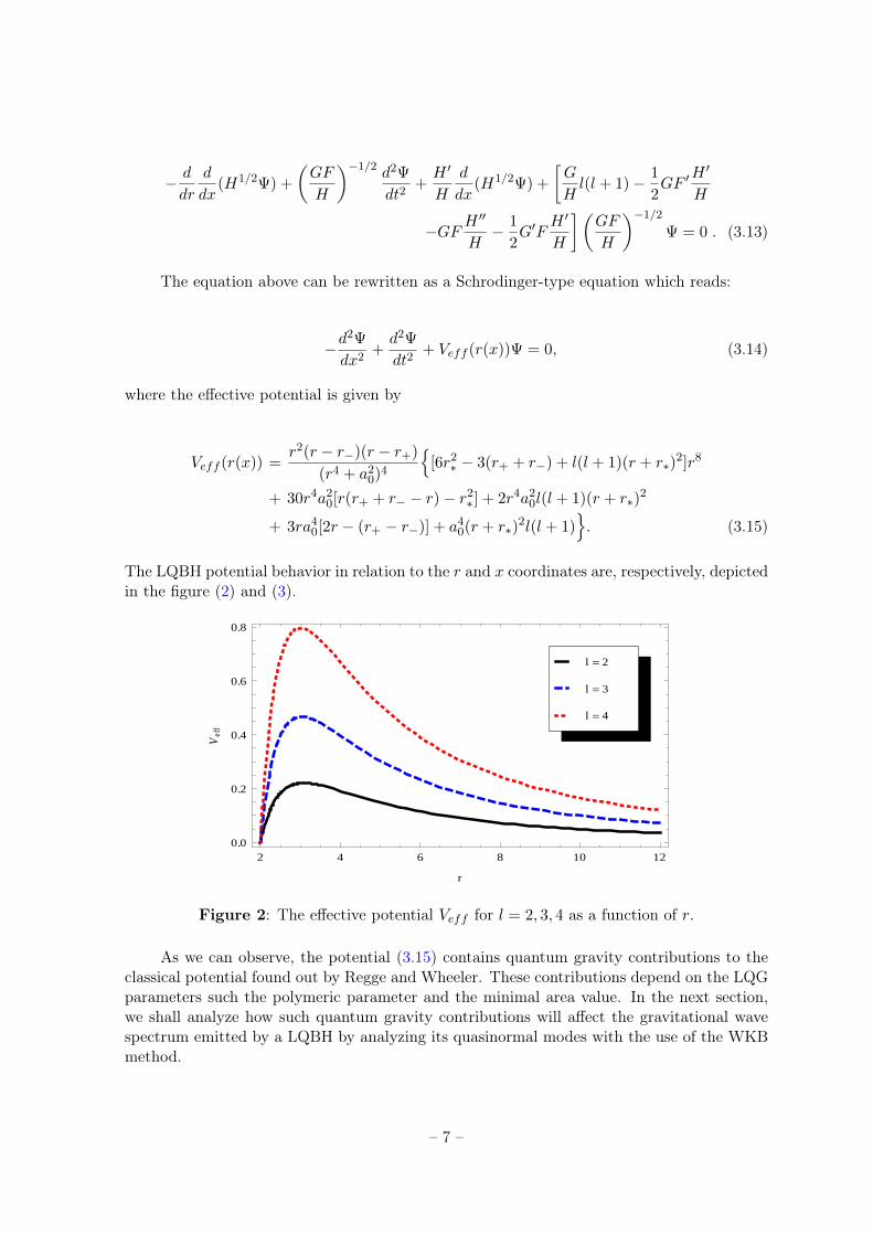
P ω0 ω1 ω2
0.1 0.8558630.1003i 0.8411430.302896i 0.8141540.510298i0.2 0.9069660.100191i 0.8940940.302316i 0.8704570.508691i0.3 0.9506180.0982154i 0.9396740.296093i 0.9194890.497559i0.4 0.98460.0941816i 0.9756130.283677i 0.9589180.476039i0.5 1.006480.0879106i 0.9993990.264553i 0.9861180.443325i0.6 1.013520.0792181i 1.008230.238192i 0.9981560.398594i0.7 1.002750.0678756i 0.9990480.203932i 0.9919080.340824i0.8 0.9712540.0533938i 0.9690330.160331i 0.9647010.267688i
Table 3: The first LQBH’s quasinormal modes for l = 4.
èè
è
è
è
è
ìì
ì
ì
ì
ì
òò
ò
ò
ò
ò
1 2 3 4 5 6
0.2
0.4
0.6
0.8
n
Re
@ΩD
ò l = 4
ì l = 3
è l = 2
(a) Real
è
è
è
è
è
è
ì
ì
ì
ì
ì
ì
ò
ò
ò
ò
ò
ò
1 2 3 4 5 6
0.2
0.4
0.6
0.8
1.0
n
-Im
@ΩD
ò l = 4
ì l = 3
è l = 2
(b) Imaginary
Figure 4: Behavior of the quasinormal modes, (a) real part and (b) imaginary part of ω forl = 2, 3, 4 and P = 0.1.
In order to visualize in a better way the effects of the quantum gravity correctionspresent in the LQBH scenario on the black hole quasinormal spectrum, we have depicted in
– 10 –
èè
è
è
è
è
ìì
ì
ì
ì
ì
ò òò
ò
ò
ò
1 2 3 4 5 6
0.3
0.4
0.5
0.6
0.7
0.8
0.9
n
Re
@ΩD
ò l = 4
ì l = 3
è l = 2
(a) Real
è
è
è
è
è
è
ì
ì
ì
ì
ì
ì
ò
ò
ò
ò
ò
ò
1 2 3 4 5 6
0.2
0.4
0.6
0.8
1.0
n
-Im
@ΩD
ò l = 4
ì l = 3
è l = 2
(b) Imaginary
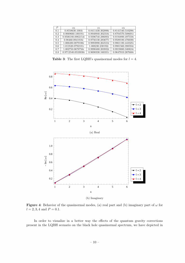
Figure 5: Behavior of the quasinormal modes, (a) real part and (b) imaginary part of ω forl = 2, 3, 4 and P = 0.3.
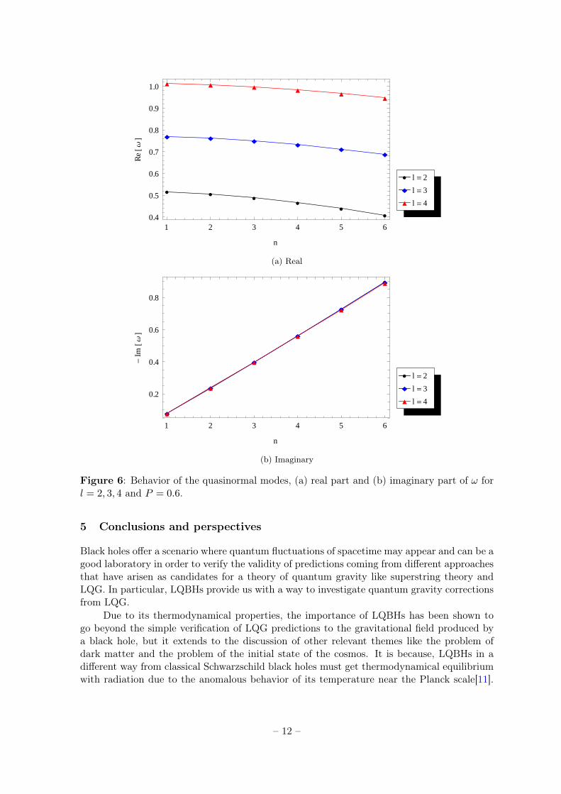
the graphics (4), (5) and (6) the behavior of the LQBH quasinormal modes, as a function ofn, for different values of the polymeric function P . In this way, we have (a) real part and (b)imaginary part of ωn for l = 2, 3, 4, by consideration of the following values of the polymericfunction: P = 0.1, P = 0.3 and P = 0.6.
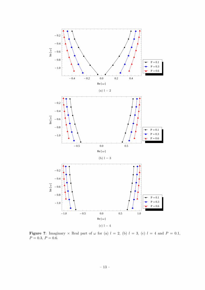
Moreover, it is interesting yet to plot the frequencies in the complex plane. In this way,in figure (7) this is done considering three families of multipoles l = 2, 3, 4. Looking at theright side of the figure, we conclude that the frequency curves are moving clockwise as Pgrows, which consists in the inverse effect we have in the case of scalar perturbations [27, 28].Such twisting effect becomes more apparent for larger values of the angular quantum number.
– 11 –
è èè
èè
è
ì ìì
ìì
ì
ò ò òò
òò
1 2 3 4 5 60.4
0.5
0.6
0.7
0.8
0.9
1.0
n
Re
@ΩD
ò l = 4
ì l = 3
è l = 2
(a) Real
è
è
è
è
è
è
ì
ì
ì
ì
ì
ì
ò
ò
ò
ò
ò
ò
1 2 3 4 5 6
0.2
0.4
0.6
0.8
n
-Im
@ΩD
ò l = 4
ì l = 3
è l = 2
(b) Imaginary
Figure 6: Behavior of the quasinormal modes, (a) real part and (b) imaginary part of ω forl = 2, 3, 4 and P = 0.6.
5 Conclusions and perspectives
Black holes offer a scenario where quantum fluctuations of spacetime may appear and can be agood laboratory in order to verify the validity of predictions coming from different approachesthat have arisen as candidates for a theory of quantum gravity like superstring theory andLQG. In particular, LQBHs provide us with a way to investigate quantum gravity correctionsfrom LQG.
Due to its thermodynamical properties, the importance of LQBHs has been shown togo beyond the simple verification of LQG predictions to the gravitational field produced bya black hole, but it extends to the discussion of other relevant themes like the problem ofdark matter and the problem of the initial state of the cosmos. It is because, LQBHs in adifferent way from classical Schwarzschild black holes must get thermodynamical equilibriumwith radiation due to the anomalous behavior of its temperature near the Planck scale[11].
– 12 –
è
è
è
è
è
è
è
è
è
è
è
è
ì
ì
ì
ì
ì
ì
ì
ì
ì
ì
ì
ì
ò
ò
ò
ò
ò
ò
ò
ò
ò
ò
ò
ò
ò
ò
- 0.4 - 0.2 0.0 0.2 0.4
-1.0
- 0.8
- 0.6
- 0.4
- 0.2
Re @ Ω D
Im@Ω
D
òòìì P = 0.6è P = 0.3è P = 0.1
ò P = 0.6
ì P = 0.3
è P = 0.1
(a) l = 2
è
è
è
è
è
è
è
è
è
è
è
è
ì
ì
ì
ì
ì
ì
ì
ì
ì
ì
ì
ì
ò
ò
ò
ò
ò
ò
ò
ò
ò
ò
ò
ò
ò
ò
- 0.5 0.0 0.5
-1.0
- 0.8
- 0.6
- 0.4
- 0.2
Re @ Ω D
Im@Ω
D
òòìì P = 0.6è P = 0.3è P = 0.1
ò P = 0.6
ì P = 0.3
è P = 0.1
(b) l = 3
è
è
è
è
è
è
è
è
è
è
è
è
ì
ì
ì
ì
ì
ì
ì
ì
ì
ì
ì
ì
ò
ò
ò
ò
ò
ò
ò
ò
ò
ò
ò
ò
-1.0 - 0.5 0.0 0.5 1.0
-1.0
- 0.8
- 0.6
- 0.4
- 0.2
Re @ Ω D
Im@Ω
D
òòìì P = 0.6è P = 0.3è P = 0.1
ò P = 0.6
ì P = 0.3
è P = 0.1
(c) l = 4
Figure 7: Imaginary × Real part of ω for (a) l = 2, (b) l = 3, (c) l = 4 and P = 0.1,P = 0.3, P = 0.6.
– 13 –

In this way, LQBHs have the necessary thermodynamical stability in order to be conceivedas possible candidates to dark matter [11, 12]. Moreover, from the form of the entropy-area relation associated with LQBHs, they have been pointed as the building blocks of aholographic description of loop quantum cosmology [13].
Gravitational waves, on the other hand have opened the doors to a new world in physicsand may establish a bridge between the quantum gravity world revealed by a black hole andexperimental investigations in gravity research. In this way, motivated by the new perspectivesopen by the detection of gravitational waves, in this work, we have investigated the stabilityof LQBHs on axial gravitational perturbations and its quasinormal spectrum.
In order to investigate how LQG quantum gravity corrections to a black hole scenariocan influence in the gravitational wave emission, we have obtained the LQBH quasinormalfrequencies by the use of the WKB approach. The Regge-Wheeler potential correspondingto the gravitational perturbations around the LQBH was obtained and the related Regge-Wheeler equation has been solved. After, the quasinormal frequencies have been obtainedby the use of 3th-order WKB approximation, demonstrating that such black holes are stableunder axial perturbations.
From the results found out, LQBHs quasinormal modes depend directly from the poly-meric parameter. Since this parameter does not suffers with the problem of mass suppression,it offers a good experimental way to detect the presence of quantum gravity imprints carriedby gravitational waves. A larger oscillation, as well as a slower damping occurs as the value ofthe polymeric parameter increases. As a result, the LQBHs decay slower when the quantumgravity contribution becomes more important.
All the results found out in this work, may strength the importance of LQBHs as possiblecandidates for dark matter and its rule to construct a holographic version of loop quantumcosmology. Additional contributions can be obtained, beyond the 3th order approximation,by the use of the methods developed by Konoplya [50] in a forthcoming analysis.
Acknowledgments
F. A. Brito and M. B. Cruz acknowledge Brazilian National Research Council by the financialsupport. C. A. S. Silva acknowledges F. A. Brito by his hospitality at Campina Grande FederalUniversity.
References
[1] B. F. Schutz and C. M. Will, “Black Hole Normal Modes: A Semianalytic Approach,”Astrophys. J. 291 (1985) L33.
[2] S. Iyer and C. M. Will, Phys. Rev. D 35, 3621 (1987).
[3] S. D. Mathur, Fortsch. Phys. 53 (2005) 793 doi:10.1002/prop.200410203 [hep-th/0502050].
[4] K. Nozari and S. Hamid Mehdipour, Europhys. Lett. 84 (2008) 20008 [gr-qc/0804.4221].
[5] C. A. S. Silva, Phys. Lett. B 677 (2009) 318 doi:10.1016/j.physletb.2009.05.031[gr-qc/0812.3171].
[6] C. A. S. Silva and R. R. Landim, Europhys. Lett. 96 (2011) 10007doi:10.1209/0295-5075/96/10007 [gr-qc/1003.3679].
[7] R. Fazeli, S.H. Mehdipour and S. Sayyadzad, Acta Phys. Polon. B 41 (2010) 2365.
[8] H. Kim, Phys. Lett. B 703 (2011) 94 doi:10.1016/j.physletb.2011.07.053 [hep-th/1103.3133].
– 14 –

[9] C. A. S. Silva and R. R. Landim, J. Phys. Conf. Ser. 490 (2014) 012012.doi:10.1088/1742-6596/490/1/012012
[10] L. Modesto, “Space-Time Structure of Loop Quantum Black Hole”, arXiv:0811.2196 [gr-qc].
[11] L. Modesto and I. Premont-Schwarz, “Self-dual Black Holes in LQG: Theory andPhenomenology”, Phys. Rev. D 80 (2009) 064041.
[12] R. G. L. Aragão, C. A. S. Silva, “Entropic corrected Newton’s law of gravitation and the loopquantum black hole gravitational atom”, Gen. Rel. Grav. 48 (2016) no 7, 83. arxiv: 1601.04993[gr-qc]
[13] C. A. S. Silva, “On the holographic basis of Quantum Cosmology,” arXiv:1503.00559 [gr-qc].
[14] T. Regge and J. A. Wheeler, Phys. Rev., 108 1063 (1957)
[15] F. J. Zerilli, “Gravitational field of a particle falling in a schwarzschild geometry analyzed intensor harmonics,” Phys. Rev. D 2 (1970) 2141.
[16] F. J. Zerilli, “Perturbation analysis for gravitational and electromagnetic radiation in areissner-nordstrom geometry,” Phys. Rev. D 9 (1974) 860.
[17] V. Moncrief, “Stability of Reissner-Nordstrom black holes,” Phys. Rev. D 10 (1974) 1057.
[18] V. Moncrief, “Odd-parity stability of a Reissner-Nordstrom black hole,” Phys. Rev. D 9 (1974)2707.
[19] S. A. Teukolsky, “Rotating black holes - separable wave equations for gravitational andelectromagnetic perturbations,” Phys. Rev. Lett. 29 (1972) 1114.
[20] S. A. Teukolsky and W. H. Press, “Perturbations of a rotating black hole. III - Interaction ofthe hole with gravitational and electromagnet ic radiation,” Astrophys. J. 193 (1974) 443.
[21] S. Chandrasekhar, The Mathematical Theory of Black Holes, Oxford University, New York(1983).
[22] E. Berti, Conf. Proc. C 0405132 (2004) 145 [gr-qc/0411025].
[23] B. P. Abbott et al. [LIGO Scientific and Virgo Collaborations], “Observation of GravitationalWaves from a Binary Black Hole Merger,” Phys. Rev. Lett. 116 (2016) no.6, 061102[arXiv:1602.03837 [gr-qc]].
[24] B. P. Abbott et al. [LIGO Scientific and Virgo Collaborations], “Astrophysical Implications ofthe Binary Black-Hole Merger GW150914,” Astrophys. J. 818 (2016) no.2, L22[arXiv:1602.03846 [astro-ph.HE]].
[25] B. P. Abbott et al. [LIGO Scientific and Virgo Collaborations], Phys. Rev. Lett. 116 (2016)no.24, 241103 doi:10.1103/PhysRevLett.116.241103 [arXiv:1606.04855 [gr-qc]].
[26] B. P. Abbott et al. [LIGO Scientific and VIRGO Collaborations], Phys. Rev. Lett. 118 (2017)no.22, 221101 doi:10.1103/PhysRevLett.118.221101 [arXiv:1706.01812 [gr-qc]].
[27] J. H. Chen and Y. J. Wang, “Complex frequencies of a massless scalar field in loop quantumblack hole spacetime,” Chin. Phys. B 20 (2011) 030401.
[28] V. Santos, R. V. Maluf and C. A. S. Almeida, “Quasinormal frequencies of self-dual blackholes,” arXiv:1509.04306 [gr-qc].
[29] C. Rovelli, “Quantum gravity,” Cambridge, UK: Univ. Pr. (2004) 455 p
[30] S. Sahu, K. Lochan and D. Narasimha, “Gravitational lensing by self-dual black holes in loopquantum gravity,” Phys. Rev. D 91 (2015) 063001 [arXiv:1502.05619 [gr-qc]].
[31] K. V. Kuchar, “Geometrodynamics of Schwarzschild black holes,” Phys. Rev. D 50 (1994) 3961[gr-qc/9403003].
– 15 –
[32] T. Thiemann and H. A. Kastrup, “Canonical quantization of spherically symmetric gravity inAshtekar’s selfdual representation,” Nucl. Phys. B 399 (1993) 211 [gr-qc/9310012].
[33] M. Campiglia, R. Gambini and J. Pullin, “Loop quantization of spherically symmetricmidi-superspaces,” Class. Quant. Grav. 24 (2007) 3649 [gr-qc/0703135].
[34] L. Modesto, “Disappearance of black hole singularity in quantum gravity,” Phys. Rev. D 70(2004) 124009 [gr-qc/0407097].
[35] I. Bengtsson, “Note on Ashtekar’s Variables in the Spherically Symmetric Case,” Class. Quant.Grav. 5 (1988) L139.
[36] M. Bojowald and H. A. Kastrup, “Quantum symmetry reduction for diffeomorphism invarianttheories of connections,” Class. Quant. Grav. 17 (2000) 3009 [hep-th/9907042].
[37] M. Bojowald and R. Swiderski, “The Volume operator in spherically symmetric quantumgeometry,” Class. Quant. Grav. 21 (2004) 4881 [gr-qc/0407018].
[38] M. Bojowald and R. Swiderski, “Spherically symmetric quantum horizons,” Phys. Rev. D 71(2005) 081501 [gr-qc/0410147].
[39] M. Bojowald and R. Swiderski, “Spherically symmetric quantum geometry: Hamiltonianconstraint,” Class. Quant. Grav. 23 (2006) 2129 [gr-qc/0511108].
[40] R. Gambini and J. Pullin, “Loop quantization of the Schwarzschild black hole,” Phys. Rev.Lett. 110 (2013) no.21, 211301 [arXiv:1302.5265 [gr-qc]].
[41] S. Hossenfelder, L. Modesto and I. Premont-Schwarz, “A Model for non-singular black holecollapse and evaporation”, Phys. Rev. D 81 (2010) 044036 [arXiv:0912.1823 [gr-qc]].
[42] E. Alesci and L. Modesto, “Particle Creation by Loop Black Holes,” Gen. Rel. Grav. 46 (2014)1656 [arXiv:1101.5792 [gr-qc]].
[43] B. Carr, L. Modesto and I. Premont-Schwarz, “Generalized Uncertainty Principle and Self-dualBlack Holes”, arXiv:1107.0708 [gr-qc].
[44] S. Hossenfelder, L. Modesto and I. Premont-Schwarz, “Emission spectra of self-dual blackholes”, arXiv:1202.0412 [gr-qc].
[45] C. A. S. Silva and F. A. Brito, “Quantum tunneling radiation from self-dual black holes,” Phys.Lett. B 725 (2013) 45, 456 [arXiv:1210.4472 [physics.gen-ph]].
[46] M. A. Anacleto, F. A. Brito and E. Passos, “Quantum-corrected self-dual black hole entropy intunneling formalism with GUP,” Phys. Lett. B 749 (2015) 181 [arXiv:1504.06295 [hep-th]].
[47] L. Rezzolla, “Gravitational waves from perturbed black holes and relativistic stars,”gr-qc/0302025.
[48] V. P. Frolov and I. D. Novikov, “Black hole physics: Basic concepts and new developments,”Fundamental theories of physics. 96
[49] H. J. Blome and B. Mashhoon, “The quasi-normal oscillations of a Schwarzschild black hole,”Phys. Lett. A. 100, 231 (1984)
[50] R. A. Konoplya and A. Zhidenko, "‘Quasinormal modes of black holes: From astrophysics tostring theory,"’ Rev. Mod. Phys. 83 (2011) 793 [arXiv:1102.4014 [qr-qc]].
[51] S. Chandrasekhar and S. L. Detweiler, "‘The quasi-normal modes of the Schwarzschild blackhole,"’ Proc. Roy. Soc. Lond. A 344 (1975) 441.
[52] C. Gundlach, R. H. Price and J. Pullin, "‘Late time behavior of stellar collapse and explosions:1. Linearized perturbations,"’ Phys. Rev. D 49 (1994) 883 [gr-qc/9307009].
[53] E. W. Leaver, "‘An Analytic representation for the quasi normal mode of Kerr black hole,"’Proc. Roy. Soc. Lond. A 402 (1985) 285.
– 16 –

[54] E. W. Leaver, "‘Quasinormal modes of Reissner-Nordestrom black holes,"’ Phys. Rev. D 41(1990) 2986.
[55] H. P. Nollert, "‘Quasinormal modes of Schwarzschild black holes: The determination ofquasinormal frequencies with very large imaginary parts,"’ Phys. Rev. D 47 (1993) 5253.
[56] E. Berti, V. Cardoso and A. O. Starinets, "‘Quasinormal modes of black holes and blackbranes,"’ Class. Quant. Grav. 26 (2009) 163001 [arXiv:0905.2975 [gr-qc]].
[57] K. D. Kokkotas and B. G. Schimidt, "‘Quasinormal modes of stars and black holes,"’ LivingRev. Rel, 2 (1999) 2 [ge-qc/9909058]
[58] H. P. Nollert, "‘TOPICAL REVIEW: Quasinormal modes: the characteristic ’sound’ of blackholes and neutrom stars,"’ Class. Quant. Grav. 16 (1999) R159.
– 17 –