graph theory and additive combinatorics lecturer: yufei zhao
TRANSCRIPT

Graph Theory and Additive Combinatorics
Lecturer: Yufei ZhaoE-mail address: [email protected]: http://yufeizhao.com/gtac/


Contents
About this document 5
Chapter 1. Introduction 91.1 Schur’s theorem . . . . . . . . . . . . . . . . . . . 91.2 Highlights from additive combinatorics . . . . . . . . . . 111.3 What’s next? . . . . . . . . . . . . . . . . . . . . 13
Chapter 2. Extremal graph theory 172.1 Mantel’s theorem: forbidding a triangle . . . . . . . . . . 172.2 Turán’s Theorem: forbidding a clique . . . . . . . . . . . 182.3 Erdős-Stone-Simonovits theorem: forbidding a general graph . 222.4 Forbidding complete bipartite graphs . . . . . . . . . . . 262.5 Constructing Ks,t-free graphs . . . . . . . . . . . . . . 312.6 Forbidding sparse bipartite graphs . . . . . . . . . . . . 37
Chapter 3. Szemerédi’s regularity lemma 413.1 Statement and proof . . . . . . . . . . . . . . . . . 413.2 Counting and removal lemmas for triangles . . . . . . . . 483.3 Property testing . . . . . . . . . . . . . . . . . . . 523.4 Proof of Roth’s theorem . . . . . . . . . . . . . . . . 533.5 Graph embedding and counting lemmas . . . . . . . . . . 563.6 Another proof of Erdős-Stone-Simonovits theorem. . . . . . 603.7 Hypergraph removal lemma and Szemerédi’s theorem . . . . 62
Chapter 4. Pseudorandom graphs 654.1 Eigenvalues . . . . . . . . . . . . . . . . . . . . . 654.2 Fourier analysis on finite abelian groups . . . . . . . . . . 684.3 Quasirandom graphs . . . . . . . . . . . . . . . . . 71
Chapter 5. Graph Limits 815.1 Introduction. . . . . . . . . . . . . . . . . . . . . 81
3
4 CONTENTS
5.2 Distances between graphs . . . . . . . . . . . . . . . 845.3 Compactness of the graphon space . . . . . . . . . . . . 905.4 Graph homomorphism inequalities . . . . . . . . . . . . 97
Chapter 6. Roth’s theorem 1076.1 Roth’s theorem in Fn3 . . . . . . . . . . . . . . . . . 1086.2 Roth’s proof of Roth’s theorem . . . . . . . . . . . . . 1116.3 Other approaches to Roth’s theorem over Fn3 . . . . . . . . 117
Chapter 7. Structure of set addition 1217.1 Definitions in additive combinatorics . . . . . . . . . . . 1217.2 Plünnecke–Ruzsa inequality . . . . . . . . . . . . . . 1227.3 Freiman’s theorem in abelian groups with bounded exponent . 1267.4 Freiman homomorphisms. . . . . . . . . . . . . . . . 1277.5 Bogolyubov’s lemma . . . . . . . . . . . . . . . . . 1347.6 Geometry of numbers . . . . . . . . . . . . . . . . . 1397.7 Proof of Freiman’s Theorem . . . . . . . . . . . . . . 1467.8 Additive Energy and the Balog-Szemerédi-Gowers Theorem . . 150
Chapter 8. The Sum-Product Problem 1578.1 Crossing number inequality . . . . . . . . . . . . . . . 1588.2 Szemerédi-Trotter and Incidence Geometry . . . . . . . . 159
References 165

About this document
These are the course notes for MIT 18.S997 Special Subject in Mathe-matics: Graph Theory and Additive Combinatorics, taught by Yufei Zhaoin Fall 2017. The notes are collectively written and edited by class partici-pants.1
This document is hosted on Overleaf, a collaborative online LaTeX edi-tor. It is viewable by everyone and editable by class participants. Overleafhas a number of features including real-time collaborative editing and LaTeXcompilation, version history control, and (optional) Git integration.
Instructions on writing and editing
(For class participants) Summary:
• Sign up to write one (or more, depending on class size) lecture(s).• Edit these notes on Overleaf for typos/improvements.• Use Piazza to ask questions and discuss more substantial edits.
Sign up to write lectures notes by putting your name and emailin the file writers.txt found in this folder (on Overleaf). Also register for anOverleaf account, so that all your edits will appear under your name (insteadof “anonymous user”). If you are registered for credit, sign up to write one (ormore, depending on class size) lecture(s), unless you are the editor-in-chief,in which case you are responsible for maintaining the overall state of thisdocument.
You should upload your write-up within three days of the lecture(and preferably before the next lecture, for Tuesday lectures). To upload,create a separate file for your notes in the class Overleaf project, and nameit “lec#.tex”, with “#” replaced by the number of the lecture you’re scribing.When writing, follow the formatting and organization conventions used inthe notes from the first lecture. Also, try to avoid using custom shortcuts.
1The idea of collaboratively created lecture notes was borrowed from Ravi Vakil’s under-graduate algebraic geometry course at Stanford.
5

6 ABOUT THIS DOCUMENT
(You can always write a first draft using your favorite shortcuts, then searchand replace them with standard commands before uploading your file toOverleaf.)
Edit the notes on Overleaf for typos/improvements (in any section).Use \todo...to add commentslike this one.
Use \todo...to add commentslike this one.
More substantial edit requests may be directed towards the writer of thesection. Feel free to use the class Piazza forum to discuss anything relatedto the course or the notes. You are responsible for making sure that yourown section(s) are in good shape.
If you make substantial edits to the project (and in particular, afteruploading the notes for a lecture), label the version you’ve just created,using the History and Revisions button at the top of the Overleaf editor.Then this version of the project can be easily retrieved later if necessary.
Piazza: https://piazza.com/mit/fall2017/18s997
Writing assignments
Lecturer: Yufei Zhao [email protected]
Editor-in-chief: Gwen McKinley [email protected]
Lec 1, 9/7: Yufei Zhao [email protected]
Lec 2, 9/12: Evan Chen [email protected]
Lec 3, 9/14: Yibo Gao [email protected]
Lec 4, 9/19: Ganesh Ajjanagadde [email protected]
Lec 5, 9/21: Morris Ang (Jie Jun) [email protected]
Lec 6, 9/26: Lisa Yang [email protected]
Lec 7, 9/28: Albert Soh [email protected]
Lec 8, 10/3: Ryan Alweiss [email protected]
Lec 9, 10/5: Matthew Brennan [email protected]
Lec 10, 10/12: Hong Wang [email protected]
Lec 11, 10/17: Linus Hamilton [email protected]
Lec 12, 10/19: Yonah Borns-Weil [email protected] / Matt Babbitt [email protected]
Lec 13, 10/24: Jake Wellens [email protected]
Lec 14, 10/26: Minjae Park [email protected]
Lec 15, 10/31: Diego Roque [email protected]
Lec 16, 11/2: Younhun Kim [email protected]
Lec 17: 11/7: Jerry Li [email protected] / Brynmor Chapman [email protected]
Lec 18: 11/9: Jonathan Tidor [email protected] / Nicole Wein [email protected]
Lec 19: 11/14: Kevin Sun [email protected] / Meghal Gupta [email protected]
Lec 20: 11/16: Pakawut Jiradilok [email protected]

ABOUT THIS DOCUMENT 7
Lec 21: 11/21 Sarah Tammen [email protected]
Lec 22: 11/28 Frederic Koehler [email protected] / Christian Gaetz [email protected]
Lec 23: 11/30 Saranesh Prembabu [email protected] / Benjamin Gunby [email protected]
Lec 24: 12/5 Vishesh Jain [email protected]
Lec 25: 12/7: Dhroova Aiylam [email protected]
Lec 26: 12/12 Paxton Turner [email protected] (last lecture)
[If you are taking the course for credit and have not
yet signed up to take notes for a lecture, please
double-up with someone for a lecture (preferably
for lectures later in the semester). Please make
arrangements among yourselves by email and make sure
that both people are fine with teaming up.]


CHAPTER 1
Introduction
§1.1 Schur’s theorem
Lec1: Yufei ZhaoIn the 1910’s, Schur attempted to prove Fermat’s Last Theorem by re-ducing the equation Xn +Y n = Zn modulo a prime p. He was unsuccessful.It turns out that, for every n, the equation has nontrivial solutions mod pfor all sufficiently large primes p, which Schur established by proving thefollowing classic result.
thm:schur Theorem 1.1 (Schur’s theorem). If the positive integers are colored with finitelymany colors, then there is always a monochromatic solution to x+y = z (i.e.,x, y, z all have the same color).
We will prove Schur’s theorem shortly. But first, let us show how todeduce the existence of solutions to Xn + Y n ≡ Zn (mod p) using Schur’stheorem.
Schur’s theorem is stated above in its “infinitary” (or qualitative) form.It is equivalent to a “finitary” (or quantitative) formulation below.
We write [N ] := 1, 2, . . . , N.
thm:schur-finitary Theorem 1.2 (Schur’s theorem, finitary version). For every positive integer rthere exists a positive integer N = N(r) such that if the elements of [N ]
are colored with r colors, then then there is a monochromatic solution tox+ y = z with x, y, z ∈ [N ].
With the finitary version, we can also ask quantitative questions such ashow big does N(r) have to be as a function of r. Such questions tend todifficult even to approximate.
Let us show that the two formulations, Theoremthm:schurthm:schur1.1 and
thm:schur-finitarythm:schur-finitary1.2, are equiva-
lent. It is clear that the finitary version of Schur’s theorem implies the infini-tary version. To see that the infinitary version implies the finitary version,fix r, and suppose that for every N there is some coloring φN : [N ]→ [r] that
9

10 1. INTRODUCTION
avoids monochromatic solutions to x + y = z. We can take an infinite sub-sequence of (φN ) such that, for every k ∈ N, the value of φN (k) stabilizes asN increases along this subsequence. Then the φN ’s, along this subsequence,converges pointwise to some coloring φ : N → [r] avoiding monochromaticsolutions to x+ y = z, but this contradicts the infinitary statement.
Let us now deduce Schur’s claim about Xn + Y n ≡ Zn (mod p).
thm:schur-fermat Theorem 1.3 (Schur). Let n be a positive integer. For all sufficiently largeprimes p, there are X,Y, Z ∈ 1, . . . , p−1 such that Xn+Y n ≡ Zn (mod p).
Proof assuming Schur’s theorem (Theoremthm:schur-finitarythm:schur-finitary1.2). We write (Z/pZ)× for the
group of nonzero residues mod p under multiplication. Let H be the sub-group of n-th powers in (Z/pZ)×. The index of H in (Z/pZ)× is at mostn. So the cosets of H partition 1, 2, . . . , p − 1 into at least n sets. Bythe finitary statement of Schur’s theorem (Theorem
thm:schur-finitarythm:schur-finitary1.2), for p large enough,
there is a solution tox+ y = z in Z
in one of the cosets of H, say aH for some a ∈ (Z/pZ)×. Since H consists ofn-th powers, we have x = aXn, y = aY n, and z = aZn for some X,Y, Z ∈(Z/pZ)×. Thus
aXn + aY n ≡ aZn (mod p).
HenceXn + Y n ≡ Zn (mod p)
as desired.
Now let us prove Theoremthm:schur-finitarythm:schur-finitary1.2 by deducing it from a similar sounding
result about coloring the edges of a complete graph. The next result is aspecial case of Ramsey’s theorem.
thm:ramsey-triangle Theorem 1.4. For every positive integer r, there is some integer N = N(r)
such that if the edges of KN , the complete graph on N vertices, are coloredwith r colors, then there is always a monochromatic triangle.
Proof. We use induction on r. Clearly N(1) = 3 works for r = 1. Let r ≥ 2
and suppose that the claim holds for r − 1 colors with N = N ′. We willprove that taking N = r(N ′ − 1) + 2 works for r colors..
Suppose we color, using r colors, the edges of a complete graph on r(N ′−1) + 2 Pick an arbitrary vertex v. Of the r(N ′ − 1) + 1 edges incident to v,

1. HIGHLIGHTS FROM ADDITIVE COMBINATORICS 11
at least N ′ edges incident to v have the same color, say red. If there is a rededge between any of these N ′ vertices, we obtain a red triangle. Otherwise,there are at most r−1 colors appearing among these N ′ vertices, so we havea monochromatic triangle by induction.
We are now ready to prove Schur’s theorem by setting up a graph whosetriangles correspond to solutions to x+ y = z, thereby allowing us to “trans-fer” the above result to the integers.
Proof of Schur’s theorem (Theoremthm:schur-finitarythm:schur-finitary1.2). Let φ : [N ] → [r] be a coloring.
Color the edges of a complete graph with vertices 1, . . . , N + 1 by giv-ing the edge (i, j) the color φ(|i− j|). By Theorem
thm:ramsey-trianglethm:ramsey-triangle1.4, if N is large enough,
then there is a monochromatic triangle, say on vertices i < j < k. Soφ(j − i) = φ(k − j) = φ(k − i). Take x = j − i, y = k − j, and z = k − i.Then φ(x) = φ(y) = φ(z) and x+ y = z, as desired.
§1.2 Highlights from additive combinatorics
The term additive combinatorics describes a rapidly growing body ofmathematics motivated by simple-to-state questions about addition and mul-tiplication of integers. Its methods are deep and far-reaching, connectingmany different areas of mathematics such as graph theory, harmonic analy-sis, ergodic theory, and discrete geometry. The rest of this section highlightssome important developments in additive combinatorics in the past century.
In the 1920’s, van der Waerden proved the following result about monochro-matic arithmetic progressions in the integers.
thm:vdw Theorem 1.5 (van der Waerden’s theorem). If the integers are colored withfinitely many colors, then one of the color classes must contain arbitrarilylong arithmetic progressions.
Remark 1.6. Having arbitrarily long arithmetic progression is very differentfrom having infinitely long arithmetic progressions. As an exercise, showthat one can color the integers using just two colors so that there are noinfinitely long monochromatic arithmetic progressions.
In the 1930’s, Erdős and Turán conjectured a stronger statement, thatany subset of the integers with positive density contains arbitrarily longarithmetic progressions. To be precise, we say that A ⊆ Z has positive upper

12 1. INTRODUCTION
density if
lim supN→∞
|A ∩ −N, . . . , N|2N + 1
> 0.
(There are several variations of this definition—the exact formulation is notcrucial.)
In the 1950’s, Roth proved the conjecture for 3-term arithmetic progres-sion using Fourier analytic methods. In the 1970’s, Szemerédi fully settledthe conjecture using combinatorial techniques. These are landmark theoremsin the field. Much of what we will discuss in this course are motivated bythese results and the developments around them.
thm:roth-intro Theorem 1.7 (Roth’s theorem). Any subset of the integers with positive up-per density contains a 3-term arithmetic progression.
thm:szemeredi-intro Theorem 1.8 (Szemerédi’s theorem). Any subset of the integers with positiveupper density contains arbitrarily long arithmetic progressions.
Szemerédi’s theorem is deep, and all known proofs are long and involved.The result led to many subsequent developments in additive combinatorics.Several different proofs of Szemerédi’s theorem have since been discovered,and some of them have blossomed into rich areas of mathematical research.Here are the most influential modern perspectives towards Szemerédi’s the-orem (in historical order):
• The ergodic theoretic approach (Furstenberg)• Higher-order Fourier analysis (Gowers)• Hypergraph regularity lemma (Rödl et al./Gowers)
The relationships between these disparate approaches are slowly beingunderstood. A unifying theme underlying all known approaches to Sze-merédi’s theorem is the dichotomy between structure and pseudorandomness,which we will see in several places in this course.
Let us mention a few other important subsequent developments to Sze-merédi’s theorem.
Instead of working over subsets of integers, let us consider subsets ofa higher dimensional lattice Zd. We say that A ⊂ Zd has positive upperdensity if lim supN→∞ |A∩ [−N,N ]d|/(2N+1)d > 0 (as before, other similardefinitions are possible). We say that A contains arbitrary constellations iffor every finite set F ⊂ Zd, there is some a ∈ Zd and t ∈ Z>0 such thata + t · F = a + tx : x ∈ F is contained in A. In other words, A contains

1. WHAT’S NEXT? 13
every finite pattern, where a pattern means a finite set up to dilation andtranslation. The following multidimensional generalization of Szemerédi’stheorem was proved by Furstenberg and Katznelson.
thm:md-sz Theorem 1.9 (Multidimensional Szemerédi theorem). Every subset of Zd ofpositive upper density contains arbitrary constellations.
There is also a polynomial extension of Szemerédi’s theorem. Let us firststate a special case, originally conjectured by Lovász and proved indepen-dently by Furstenberg and Sárkőzy.
thm:sarkozy Theorem 1.10. Any subset of the integers with positive upper density con-tains two numbers differing by a square.
In other words, the set always contains x, x + y2 for some x ∈ Z andy ∈ Z>0. What about other polynomial patterns? The following polynomialgeneralization was proved by Bergelson and Leibman.
thm:poly-sz Theorem 1.11 (Polynomial Szemerédi theorem). Suppose A ⊂ Z has positiveupper density. If P1, . . . , Pk ∈ Z[X] are polynomials with P1(0) = · · · =
Pk(0) = 0, then there exist x ∈ Z and y ∈ Z>0 such that x+ P1(y), . . . , x+
Pk(y) ∈ A.
We leave it as an exercise to formulate a common extension of the abovetwo theorems (i.e., a multidimensional polynomial Szemerédi theorem). Sucha theorem was also proved by Bergelson and Leibman.
We will not cover the proof of Theoremsthm:md-szthm:md-sz1.9 and
thm:poly-szthm:poly-sz1.11 in this course. In
fact, currently the only known proof of Theoremthm:poly-szthm:poly-sz1.11 uses ergodic theory,
which is beyond the scope of this course.Another groundbreaking development is the following famous result of
Green and Tao, which settled an old folklore conjecture about prime num-bers.
thm:green-tao Theorem 1.12 (Green–Tao theorem). The primes contain arbitrarily long arith-metic progressions.
§1.3 What’s next?
An important goal of this course is to understand two different proofs ofRoth’s theorem, which can be rephrased as:

14 1. INTRODUCTION
Roth’s theorem: Every subset of [N ] that does not contain3-term arithmetic progressions has size o(N).
Roth originally proved his result using Fourier analytic techniques, whichwe will see in the second half of this course. In the 1970’s, leading up toSzemerédi’s proof of his landmark result, Szemerédi developed an importanttool known as the graph regularity lemma. He and Ruzsa used the graphregularity lemma to give a new, graph theoretic proof of Roth’s theorem.One of the first goals of this course will be to understand this graph theoreticproof.
As in the proof of Schur’s theorem, we will formulate a graph theoreticproblem whose solution implies Roth’s theorem. This topic fits nicely in anarea of combinatorics called extremal graph theory. A starting point (alsofor us) in extremal graph theory is the following question:
What is the maximum number of edges in a triangle-freegraph on n vertices?
This question is relatively easy, and it was answered by Mantel in the early1900’s (and subsequently rediscovered and generalized by Turán). It will bethe first result that we shall prove next. However, even though it soundssimilar to Roth’s theorem, it cannot be used to deduce Roth’s theorem.Later on, we will construct a graph that corresponds to Roth’s theorem, andit turns out that the right question to ask is:
What is the maximum number of edges in an n-vertexgraph where every edge is contained in a unique triangle?
We do not know the exact answer, but we will prove, using Szemerédi’sregularity lemma, that that any such graph must have o(n2) edges. Roth’stheorem would then follow.
Notes
Schur’s results (Theoremsthm:schurthm:schur1.1–
thm:schur-fermatthm:schur-fermat1.3) were proved in [44].
Theoremthm:ramsey-trianglethm:ramsey-triangle1.4 is a special case of Ramsey’s theorem [34], which tells us
that for every k, r, s, there is some N such that if the edges of a k-uniformhypergraph on N are colored with r colors, then there is a monochromaticclique on s vertices.
van der Waerden’s theorem (Theoremthm:vdwthm:vdw1.5) was proved in [54]. Erdős
and Turán [15] conjectured that the real reason for van der Waerden’s the-orem is that some color class has positive density. Settling the Erdős–Turán

1. WHAT’S NEXT? 15
conjecture, Roth [40] proved it for 3-term arithmetic progressions (Theo-rem
thm:roth-introthm:roth-intro1.7), and Szemerédi [50] proved it for 4-term arithmetic progressions
and subsequently [51] for k-term arithmetic progressions for any k. Therehave been several different proofs of Szemerédi’s theorem that have beenquite influential. Furstenberg [18] (see also [19,21]) proved an ergodic the-oretic result that is equivalent to Szemerédi’s theorem. Gowers [22] general-ized Roth’s Fourier analytic approach to longer arithmetic progressions andsignificantly improved early bounds on Szemerédi’s theorem for longer pro-gressions. Rödl et al. [32,35–39] and independently Gowers [23] generalizedthe graph regularity lemma to hypergraphs, and gave a new combinatorialproof of Szemerédi’s theorem.
The multidimensional Szemerédi theorem (Theoremthm:md-szthm:md-sz1.9) was initially
proved by Furstenberg and Katznelson [20] using ergodic theory. The firstnon-ergodic theoretic proof was via the hypergraph regularity lemma men-tioned above.
Theoremthm:sarkozythm:sarkozy1.10 was conjectured by Lovász and proved independently by
Furstenberg [18] (via ergodic theory) and by Sárkőzy [42] (using Fourieranalytic methods). The polynomial Szemerédi theorem (Theorem
thm:poly-szthm:poly-sz1.11) was
proved by Bergelson and Leibman [5] using ergodic theory, and no otherproof is currently known (except in some special cases, e.g., [33]).
The Green–Tao theorem was proved in [24].Ruzsa and Szemerédi [41] proved the triangle removal lemma using the
graph regularity lemma [52]. This gives a graph theoretic proof of Roth’stheorem.


CHAPTER 2
Extremal graph theorych:extremal-graph-theory
Lec2: Evan Chen
§2.1 Mantel’s theorem: forbidding a triangle
We start with the following question.
What is the maximum number of edges in an n-vertextriangle-free graph?
These type of questions is the focus of this chapter. Namely we are interestedin understanding extremal graphs while forbidden certain substructures.
thm:mantel Theorem 2.1 (Mantel’s theorem). If a graph G on n vertices contains notriangles, then it has at most n2/4 edges.
Remark 2.2. The extremal example is to take a complete bipartite graphKbn/2c,dn/2e. It is easy to see that bipartite graphs are triangle-free. Thisgraph has
⌊n2/4
⌋edges. Thus the bound in Mantel’s theorem is tight.
bn/2c dn/2e
We give two different proofs of this theorem. They illustrate differentideas.
First proof of Theoremthm:mantelthm:mantel2.1. Suppose G has m edges. We use the notation
d(x) for the degree of the vertex x.
17

18 2. EXTREMAL GRAPH THEORY
Observe that if x is adjacent to y in G, then every other vertex otherthan x, y cannot be adjacent to both x and y. Consequently,
d(x) + d(y) ≤ n for every edge xy of G.
Sum over all edges, we obtain∑xy∈E(G)
(d(x) + d(y)) ≤ mn.
On the left-hand side, for every vertex x ∈ V (G), the term d(x) appearsonce for each edge incident to x, i.e., d(x) times in total. Thus the left-handside is equal to
∑x∈V (G) d(x)2. It follows that∑
x∈V (G)
d(x)2 ≤ mn.
Now by the Cauchy-Schwarz inequality, we have
(2m)2 =
(∑x
d(x)
)2
≤ n(∑
x
d(x)2
)≤ mn2.
Second proof of Theoremthm:mantelthm:mantel2.1. Let A be an independent set of maximum size
in G.Since G is triangle-free, the neighborhood of any vertex is an indepen-dent set, so d(x) ≤ |A| for all x ∈ V (G).
On the other hand, let B = V (G) \ A. Since A is independent, everyedge of G must have at least one endpoint in B. So
e(G) ≤∑x∈B
d(x) ≤∑x∈B|A| = |A||B| ≤
( |A|+ |B|2
)2
=n2
4.
Remark 2.3. By checking the equality conditions in the second proof, wesee that Kbn/2c,dn/2e is the unique triangle-free with the maximum number⌊n2/4
⌋number of edges..
Remark 2.4. The proof above works equally well if we replace A by theneighborhood of any maximum degree vertex of G.
§2.2 Turán’s Theorem: forbidding a cliquesec:extremal-turan
We now consider the following generalization:
What’s the maximum number of edges in an n-vertex graphthat does not contain a clique on r + 1 vertices?
We begin by constructing the following example.

2. TURÁN’S THEOREM: FORBIDDING A CLIQUE 19
def:turan-graph Definition 2.5. Let the Turán graph Tn,r be the n-vertex graph obtained bypartitioning the vertex set into parts of sizes either bn/rc or dn/re and anedge between any pair of vertices lying in different parts.
Note that there is a unique way to partition n vertices into parts of sizesdiffering by at most 1.
thm:turan Theorem 2.6 (Turán’s Theorem). If G is an n-vertex graph with no copiesof Kr+1 then it has at most e(Tn,r) edges.
We will give three proofs.
First proof of Theoremthm:turanthm:turan2.6. (By induction) We proceed by induction on the
number of vertices n. The result is trivial when n ≤ r. So assume n > r
from now on.Let G be a Kr+1-free graph on n vertices with the possible maximum
number of edges. ThenG contains a copy ofKr (otherwise we adding anotheredge to G would still make it Kr+1-free). Let A a set of r vertices of Gforming a clique and let B = V (G) \A.
v
A
B
Then every vertex in B is adjacent to at most r − 1 vertices in A, orelse this vertex together with B forms a copy of Kr+1. 1 There are
(r2
)1At this point it’s important to remark that we are really “already done” — we have acalculation which is going to be tight at the equality case (we are just deleting a single Kr
from Tn,r). So even before completing the calculation, we know we should get the exactquantity.

20 2. EXTREMAL GRAPH THEORY
edges within A, at most (r − 1)|B| edges between A and B by the aboveobservation, and at most e(Tn−r, r) in B by induction. Thus
e(G) ≤(r
2
)+ (r − 1)|B|+ eG(B)
=
(r
2
)+ (r − 1)(n− r) + e(Tn−r,r)
= e(Tn,r),
where the final step can be observed by noting that one can obtain Tn−r,rfrom Tn by removing a vertex from each of the r vertex parts.
Second proof of Theoremthm:turanthm:turan2.6. (By Zykov symmetrization) Let G be an n-
vertex Kr+1-free graph with the maximum possible number of edges. Wewill show that
For any x, y, z ∈ V (G), if xy /∈ E(G) and yz /∈ E(G), thenxz /∈ E(G).
Assume this is not true, so xy, yz /∈ E(G) but xz ∈ E(G).
x
y
z
Suppose first that d(y) < d(x). Then we replace y by a “clone” x′ of x,connected to exactly the neighbors of x.
x
y ⇒x
x′
Then the number of edges increases, and the graph remains still Kr+1-free(note that there is no edge between x and x′). Thus, we may assume d(x) ≤d(y). Similarly, we may assume d(z) ≤ d(y).
Now let G′ be the graph obtained from G by replacing both x and z beclones of y. Then G′ is Kr+1-free. Since we added 2d(y) edges and removed
2. TURÁN’S THEOREM: FORBIDDING A CLIQUE 21
d(x) + d(z)− 1 edges,
e(G′) = e(G) + 2d(y)− (d(x) + d(z)− 1) > e(G).
This contradicts the assumption that G has the maximum number of edgesamong n-vertex Kr+1-free graphs. Therefore, we must have xz ∈ E(G), thusproving the claim above.
It follows that non-adjacency (i.e., xy /∈ E(G)) in G is an equivalencerelation, so that the complement of G is a disjoint union of cliques. HenceG must be a complete multipartite graph with at most r parts. The parts ofG must have sizes differing by at most one, since if two parts differ in morethan one vertex in size, then moving a vertex from the bigger part to thesmaller part increases the number of edges. It follows that G must be theTurán graph Tn,r.
Remark 2.7. Both the first and second proof also show that the Turán graphTn,r is the unique graph achieving the maximum number of edges.
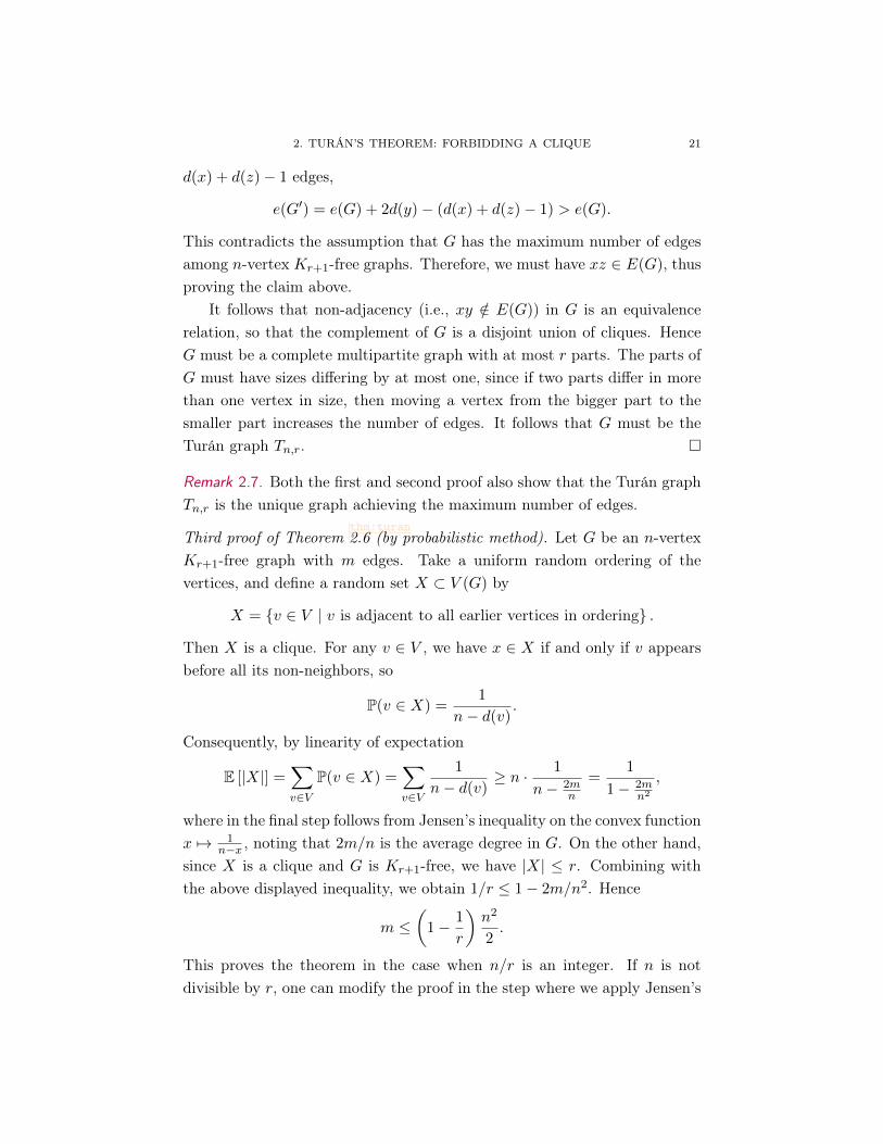
Third proof of Theoremthm:turanthm:turan2.6 (by probabilistic method). Let G be an n-vertex
Kr+1-free graph with m edges. Take a uniform random ordering of thevertices, and define a random set X ⊂ V (G) by
X = v ∈ V | v is adjacent to all earlier vertices in ordering .
Then X is a clique. For any v ∈ V , we have x ∈ X if and only if v appearsbefore all its non-neighbors, so
P(v ∈ X) =1
n− d(v).
Consequently, by linearity of expectation
E [|X|] =∑v∈V
P(v ∈ X) =∑v∈V
1
n− d(v)≥ n · 1
n− 2mn
=1
1− 2mn2
,
where in the final step follows from Jensen’s inequality on the convex functionx 7→ 1
n−x , noting that 2m/n is the average degree in G. On the other hand,since X is a clique and G is Kr+1-free, we have |X| ≤ r. Combining withthe above displayed inequality, we obtain 1/r ≤ 1− 2m/n2. Hence
m ≤(
1− 1
r
)n2
2.
This proves the theorem in the case when n/r is an integer. If n is notdivisible by r, one can modify the proof in the step where we apply Jensen’s

22 2. EXTREMAL GRAPH THEORY
inequality, noting that, given∑
v d(v), the expression∑
v∈V 1/(n − d(v))isminimized, if the numbers d(v) are as close to each other as possible (hencediffering by at most one from each other). The rest of the analysis is straight-forwards, so we omit the details.
§2.3 Erdős-Stone-Simonovits theorem: forbidding a generalgraph
In Mantel’s theorem and Turán’s theorem, we considered the problem ofdetermining the maximum of edges in a graph without a clique of given size.We will generalize this notion by forbidding an arbitrary subgraph.
def:ex Definition 2.8. Let ex(n,H) denote the maximum number of edges in an n-vertex graph that does not contain a copy of H.
Remark 2.9. In the above definition, we do not require the copy of H to bean induced subgraph. We say that H is a subgraph of G if H is obtainedfrom G by taking a subset of vertices and a subset of edges between thosevertices. On the other hand, we say that H is an induced subgraph of G ifH is obtained from G by taking a subset of the vertices along with all edgesof G between those vertices.
For example, C4, the cycle on four vertices, is a subgraph of K4, but notas an induced subgraph.
Generally, we only mean induced when we explicitly use the word “in-duced.”
With this notation, Turán’s theorem can be restated as
ex (n,Kr+1) = e(Tn,r)
It is worth noting that
ex (n,Kr+1) ≤(
1− 1
r
)n2
2
and
ex (n,Kr+1) =
(1− 1
r+ o(1)
)n2
2for fixed r, as n→∞.
Perhaps surprisingly, it is possible to determine the asymptotic behaviorof ex(n,H) for a large class of graphs H simply using the chromatic numberof H.
2. ERDŐS-STONE-SIMONOVITS THEOREM: FORBIDDING A GENERAL GRAPH 23
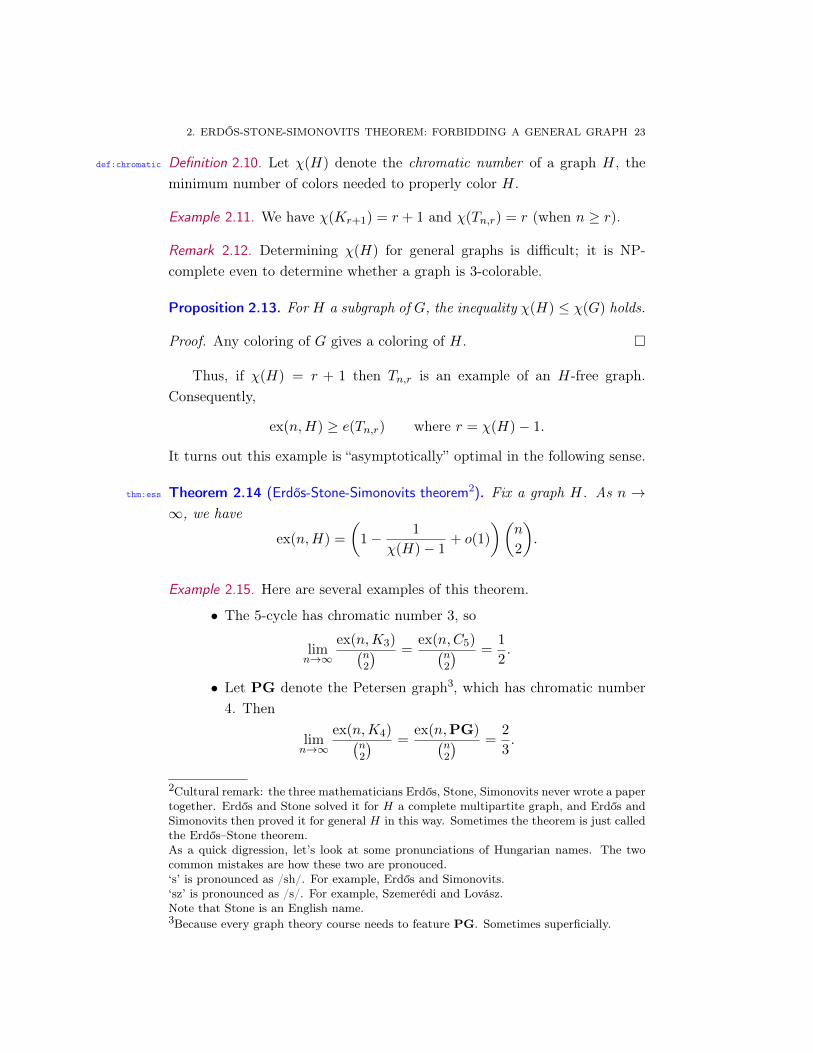
def:chromatic Definition 2.10. Let χ(H) denote the chromatic number of a graph H, theminimum number of colors needed to properly color H.
Example 2.11. We have χ(Kr+1) = r + 1 and χ(Tn,r) = r (when n ≥ r).
Remark 2.12. Determining χ(H) for general graphs is difficult; it is NP-complete even to determine whether a graph is 3-colorable.
Proposition 2.13. For H a subgraph of G, the inequality χ(H) ≤ χ(G) holds.
Proof. Any coloring of G gives a coloring of H.
Thus, if χ(H) = r + 1 then Tn,r is an example of an H-free graph.Consequently,
ex(n,H) ≥ e(Tn,r) where r = χ(H)− 1.
It turns out this example is “asymptotically” optimal in the following sense.
thm:ess Theorem 2.14 (Erdős-Stone-Simonovits theorem2). Fix a graph H. As n →∞, we have
ex(n,H) =
(1− 1
χ(H)− 1+ o(1)
)(n
2
).
Example 2.15. Here are several examples of this theorem.
• The 5-cycle has chromatic number 3, so
limn→∞
ex(n,K3)(n2
) =ex(n,C5)(
n2
) =1
2.
• Let PG denote the Petersen graph3, which has chromatic number4. Then
limn→∞
ex(n,K4)(n2
) =ex(n,PG)(
n2
) =2
3.
2Cultural remark: the three mathematicians Erdős, Stone, Simonovits never wrote a papertogether. Erdős and Stone solved it for H a complete multipartite graph, and Erdős andSimonovits then proved it for general H in this way. Sometimes the theorem is just calledthe Erdős–Stone theorem.As a quick digression, let’s look at some pronunciations of Hungarian names. The twocommon mistakes are how these two are pronouced.‘s’ is pronounced as /sh/. For example, Erdős and Simonovits.‘sz’ is pronounced as /s/. For example, Szemerédi and Lovász.Note that Stone is an English name.3Because every graph theory course needs to feature PG. Sometimes superficially.

24 2. EXTREMAL GRAPH THEORY
The equality case is to take Tn,3 the point is that PG can’t beembedded into Tn,3 by virtue of not being 3-colorable.
6→Remark 2.16. Note that if χ(H) = 2, the theorem only implies that ex(n,H) =
o(n2), which is much less satisfying. For most bipartite graphs H it is stillopen what the leading term of ex(n,H) is.
The proof of Theoremthm:essthm:ess2.14 begins with the following lemma with a very
general and useful idea. A powerful general message is that having “high”average often implies that we can find a “large” subset with “high” mini-mum. The specific quantifications depend on the applications in mind. Inthe following lemma, we transform a graph with high average degree into asubgraph with a high minimum degree, and this is done by removing lowdegree vertices one at a time.
lem:avgtomindeg Lemma 2.17. Whenever 0 < ε < δ, for all n sufficiently large in terms of εand δ, if G is an n-vertex graph with average degree at least δn then thereexists a subgraph G′ of G on n′ ≥
√ε
2 n vertices and with minimum degree atleast (δ − ε)n′.
Proof.Lec3: Yibo Gao Let G0 = G. Construct G1, G2, . . . by successively removing minimaldegree vertices one at a time. If min deg(Gi) ≥ (δ − ε)(n− i), then we stopthe process. We will show that by the time we stop, there are still a lot ofvertices remaining. Suppose we stop at Gn−n′ (after n − n′ steps) with n′
vertices remaining. Then,
#edges removed <n∑
k=n′+1
(δ − ε)k = (δ − ε)(n+ n′ + 1)(n− n′)2
.
Since G has average degree at least δn,
δn2
2≤ e(G) ≤e(Gn−n′) + (δ − ε)(n+ n′ + 1)(n− n′)
2
≤(n′
2
)+ (δ − ε)(n+ n′ + 1)(n− n′)
2.
2. ERDŐS-STONE-SIMONOVITS THEOREM: FORBIDDING A GENERAL GRAPH 25
Rearranging, we obtain
εn2
2− (δ − ε)n
2≤(n′
2
)− (δ − ε)n
′(n′ + 1)
2.
Thus, if n is large enough depending on δ and ε, the first quadratic term isdominant. We find that n′ ≥
√ε
2 n as a result. The resulting graph G′ =
Gn−n′ has minimum degree at least (δ − ε)n′ by our construction.
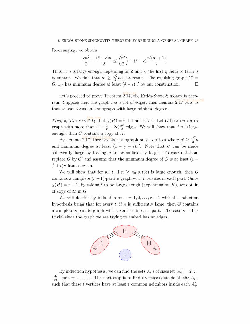
Let’s proceed to prove Theoremthm:essthm:ess2.14, the Erdős-Stone-Simonovits theo-
rem. Suppose that the graph has a lot of edges, then Lemmalem:avgtomindeglem:avgtomindeg2.17 tells us
that we can focus on a subgraph with large minimal degree.
Proof of Theoremthm:essthm:ess2.14. Let χ(H) = r + 1 and ε > 0. Let G be an n-vertex
graph with more than (1− 1r + 2ε)n
2
2 edges. We will show that if n is largeenough, then G contains a copy of H.
By Lemmalem:avgtomindeglem:avgtomindeg2.17, there exists a subgraph on n′ vertices where n′ ≥
√ε
2 n
and minimum degree at least (1 − 1r + ε)n′. Note that n′ can be made
sufficiently large by forcing n to be sufficiently large. To ease notation,replace G by G′ and assume that the minimum degree of G is at least (1−1r + ε)n from now on.
We will show that for all t, if n ≥ n0(s, t, ε) is large enough, then G
contains a complete (r+ 1)-partite graph with t vertices in each part. Sinceχ(H) = r + 1, by taking t to be large enough (depending on H), we obtainof copy of H in G.
We will do this by induction on s = 1, 2, . . . , r + 1 with the inductionhypothesis being that for every t, if n is sufficiently large, then G containsa complete s-partite graph with t vertices in each part. The case s = 1 istrivial since the graph we are trying to embed has no edges.
tA1
t
t
As
t
By induction hypothesis, we can find the sets Ai’s of sizes let |Ai| = T :=
d 4trεe for i = 1, . . . , s. The next step is to find t vertices outside all the Ai’s
such that these t vertices have at least t common neighbors inside each A′i.

26 2. EXTREMAL GRAPH THEORY
Let’s count cliques (v1, v2, . . . , vs, w) where v1 ∈ A1, . . . , vs ∈ As, w /∈A1 ∪ · · · ∪ As. For any (v1, . . . , vs) ∈ A1 × · · · × As, the number of choicesfor w is at least
n− s(
1
r− ε)n− |A1 ∪ · · · ∪As| ≥ n− r
(1
r− ε)n− sT
≥ rεn
2,
for n sufficiently large (depending on r, ε, and T ). Thus, the number of suchcliques is at least rεn
2 |A1| · · · |As|. Let W ⊂ V \ (A1 ∪ · · · ∪As) be the set ofw’s that appears in at least rε
4 |A1| · · · |As| such cliques. We then haverεn
2|A1| · · · |As| ≤ |W | · |A1| · · · |As|+ n · rε
4· |A1| · · · |As|.
Therefore, |W | ≥ rε4 n. Note that every vertex inW has at least rε
4 |Ai| neigh-bors in each Ai, for i = 1, . . . , s. (Otherwise, w is in less than rε
4 |A1| · · · |An|cliques.) There are
(Tt
)sways to select a t-element subset from each Ai. By
the pigeonhole principle, if n is large enough, there exist B1 ⊂ A1, . . . , Bs ⊂As with |Bi| = t such that there exist t different vertices inW , each adjacentto all vertices in B1, . . . , Bs. This completes an (s+ 1)-partite graph with tvertices in each part.
We will see another proof in Chapterch:regularitych:regularity3 after developing Szemerédi’s
regularity lemma.
§2.4 Forbidding complete bipartite graphs
The Erdős-Stone-Simonovits theorem tells us that ex(n,H) = o(n2) forbipartite H (as χ(H) = 2), but this result does not tell us the precise as-ymptotic rate of growth of ex(n,H). For most bipartite graphs, the order ofgrowth of ex(n,H) is unknown. We will see some upper and lower bounds,and a few cases where we can determine ex(n,H) up to a constant factor.
The most well-known case is the complete bipartite graphKs,t. In partic-ular, every bipartite graph is contained in Ks,t for some s, t. So the extremalnumber of every bipartite graph is bounded by the extremal number of com-plete bipartite graphs ex(n,H) ≤ ex(n,Ks,t).
prob:zar Problem 2.18 (Zarankiewicz problem). Determine ex(n,Ks,t).
The problem remains open for general s, t. Here is an upper bound thathas been conjectured to be tight up to a constant factor.

2. FORBIDDING COMPLETE BIPARTITE GRAPHS 27
thm:kst Theorem 2.19 (Kővári-Sós-Turán theorem). Fix positive integers s ≤ t. Thereexists constant C such that
ex(n,Ks,t) ≤ Cn2− 1s .
For certain values of s and t, we will construct matching lower boundconstructions (up to a constant factor). This is perhaps evidence that theupper bound is tight in general, in which case the current difficulty lies infinding good constructions of Ks,t-free graphs.
Proof. The proof is done via a double counting argument. Suppose G isKs,t-free with n vertices and m edges. Let T be the number of copies of Ks,1
in G. We bound T from above and from below.Since G is Ks,t free so every set of s vertices has at most t− 1 common
neighbors. This gives T ≤ (t− 1)(ns
).
Letting d(v) denote the degree of v, we have
T =∑
v∈V (G)
(d(v)
s
)≥ n
( 1n
∑v d(v)
s
)= n
(2m/n
s
)by convexity of the function p(x) =
(xk
)= x(x − 1) · · · (x − k + 1)/k! for
x ≥ k.4Combining the upper and lower bounds on T , we find,
(1 + o(1))n(2m/n)s
s!= n
(2m/n
s
)≤ (t− 1)
(n
s
)= (1 + o(1))(t− 1)
ns
s!
where we can view s, t as constants and let n→∞. This implies
m ≤ (1 + o(1))1
2(t− 1)
1sn2− 1
s .
Lec4: GaneshAjjanagadde
Let us examine a geometric application of the Kővári-Sós-Turán theorem.The following problem, known as the unit distance problem, was originallyposed by Erdős [14]:
prob:unit_distance Problem 2.20 (Unit distance problem). Determine u(n), the maximum num-ber of times distance 1 occurs among n points placed in R2.
For small n, Schade [43] obtained the following results by determiningthe extremal sets up to isomorphism:
4Notice that the roots of p(x) are 0, 1, . . . , k − 1 so p′(x) has exactly one root in eachinterval (0, 1), (1, 2), . . . , (k − 1, k) due to the degree of the polynomial. Similarly, eachroot of p′′(x) lies between two adjacent roots of p′(x). It follows that p′′(x) > 0 for x ≥ k.
28 2. EXTREMAL GRAPH THEORY
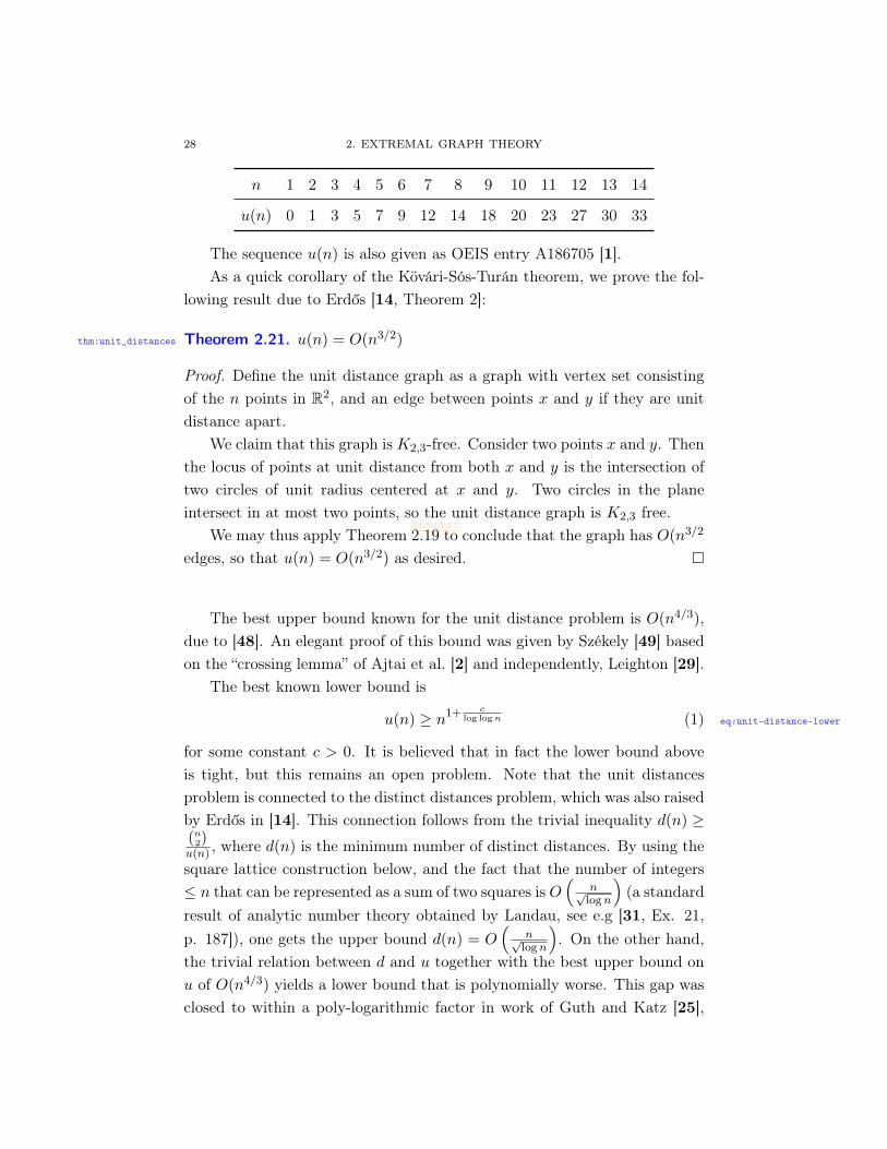
n 1 2 3 4 5 6 7 8 9 10 11 12 13 14
u(n) 0 1 3 5 7 9 12 14 18 20 23 27 30 33
The sequence u(n) is also given as OEIS entry A186705 [1].As a quick corollary of the Kövári-Sós-Turán theorem, we prove the fol-
lowing result due to Erdős [14, Theorem 2]:
thm:unit_distances Theorem 2.21. u(n) = O(n3/2)
Proof. Define the unit distance graph as a graph with vertex set consistingof the n points in R2, and an edge between points x and y if they are unitdistance apart.
We claim that this graph isK2,3-free. Consider two points x and y. Thenthe locus of points at unit distance from both x and y is the intersection oftwo circles of unit radius centered at x and y. Two circles in the planeintersect in at most two points, so the unit distance graph is K2,3 free.
We may thus apply Theoremthm:kstthm:kst2.19 to conclude that the graph has O(n3/2
edges, so that u(n) = O(n3/2) as desired.
The best upper bound known for the unit distance problem is O(n4/3),due to [48]. An elegant proof of this bound was given by Székely [49] basedon the “crossing lemma” of Ajtai et al. [2] and independently, Leighton [29].
The best known lower bound is
u(n) ≥ n1+ clog logn (1) eq:unit-distance-lower
for some constant c > 0. It is believed that in fact the lower bound aboveis tight, but this remains an open problem. Note that the unit distancesproblem is connected to the distinct distances problem, which was also raisedby Erdős in [14]. This connection follows from the trivial inequality d(n) ≥(n2)u(n) , where d(n) is the minimum number of distinct distances. By using thesquare lattice construction below, and the fact that the number of integers≤ n that can be represented as a sum of two squares is O
(n√
logn
)(a standard
result of analytic number theory obtained by Landau, see e.g [31, Ex. 21,p. 187]), one gets the upper bound d(n) = O
(n√
logn
). On the other hand,
the trivial relation between d and u together with the best upper bound onu of O(n4/3) yields a lower bound that is polynomially worse. This gap wasclosed to within a poly-logarithmic factor in work of Guth and Katz [25],

2. FORBIDDING COMPLETE BIPARTITE GRAPHS 29
who obtained d(n) = Ω(
nlogn
). A recent survey of the unit distance problem
is provided in [53].The rest of this section gives a proof of the lower bound (
eq:unit-distance-lowereq:unit-distance-lower1) to u(n). It
uses basic analytic number theory, and should be considered tangential tothe rest of the course (it was not covered in lecture).
Before getting into the details, we first sketch the argument of the lowerbound, emphasizing the key idea. The proof of the lower bound uses thegraph consisting of the integer square lattice of size ≈ √n ×√n. We focuson a distance
√r such that r has a relatively large number of representations
as a sum of squares, and such that r = o(n). This will guarantee that foressentially every vertex of the lattice (basically the vertices in the interiorwhich has side length ≈ √n − √r), there are at least n
clog logn neighbors at
that distance. Exact details of this argument hinge on two ingredients fromnumber theory:
(1) The number of representations of an integer r as a sum of two squares.This may be encapsulated in the following lemma (due to Lagrange):
lem:count_rep_sum_of_squares Lemma 2.22. Let r have prime factorization r = 2e∏ki=1 p
aii
∏lj=1 q
bjj where
the pi are distinct primes of the form 4t+1, and the qj are distinct primes ofthe form 4t+3. If one or more of the bj are odd, then r has no representationas a sum of squares. If all the bj are even, then the number of representationsof r as a sum of squares (all representations, including negative integers) is:N(r) = 4
∏ki=1(ai + 1).
Proof. The proof of this result is outside the scope of this course, but iselementary and may be found in many references on number theory, e.g [26,Theorem 278].
(2) From the above Lemmalem:count_rep_sum_of_squareslem:count_rep_sum_of_squares2.22, it is clear that a “good” r is one which is
o(n), is odd and lacks divisors of the form 4t+3 (since they don’t contributeto the number of representations). Thus, the heart of the matter is getting ahandle on how many primes of the form 4t+1 are there below a given number.What is thus needed is an analog of the celebrated prime number theorem,generalized to arithmetic progressions. Note that Dirichlet’s theorem on theinfinitude of primes in arithmetic progressions is insufficient here, as it doesnot give quantitative estimates. Also note that the Euclidean method, whichcan be used to deduce that there are infinitely many primes of the form 4t+3,and which moreover yields (weak) quantitative estimates, does not work for
30 2. EXTREMAL GRAPH THEORY
4t+ 1. As such, one essentially needs the full strength of the prime numbertheorem for arithmetic progressions:
lem:pnt_ap Lemma 2.23. Let p denote a prime number. Let
πn,a(x) = |p : p ≤ x, p ≡ a (mod n)| .
Then if a, n are coprime, we have: πn,a(x) ≈ 1φ(n)
xlog x , where φ(n) is Euler’s
totient function. One has the equivalent form ψ(x;n, a) ≈ xφ(n) , where:
ψ(x;n, a) =∑
i≤x,i≡a (mod n)
Λ(i)
=∑
p≤x,p≡a (mod n)
⌊logp x
⌋log p.
Here ψ is the Chebyshev function, and Λ the von-Mangoldt function.
Proof. This is a classic result of analytic number theory, and may be foundin references such as [10, Chapter 20]. For a relatively simple, standaloneexposition, one may see [47].
With these remarks in place, we turn to the proof of (eq:unit-distance-lowereq:unit-distance-lower1). We first
prove the lower bound by elaborating upon the sketch given above. Considerr =
∏p≤c logn,p≡1 (mod 4) p for a c > 0. By Lemma
lem:pnt_aplem:pnt_ap2.23 and
lem:count_rep_sum_of_squareslem:count_rep_sum_of_squares2.22, we see that
the number of representations of r as a sum of squares of nonnegative integers
is 2Ω(
lognlog logn
)= n
Ω(
1log logn
). Also by
lem:pnt_aplem:pnt_ap2.23,
log r ≤∑
p≤c logn,p≡1 (mod 4)
log p
≤ ψ(c log n; 4, 1) ≈ c
2log n.
Thus, for c small enough, r = o(n). Now consider the set of points P =(x, y) ∈ Z2 : 0 ≤ x, y ≤ b√nc
, and its “interior”
Po =
(x, y) ∈ Z2 : 0 ≤ x, y ≤⌊√
n⌋−⌈√
r⌉.
Then, for each point in Po, we have by the above nΩ(
1log logn
)neighbors at
distance√r. Now as |Po| ≈ |P|, we get the desired lower bound u(n) ≥
n1+Ω
(1
log logn
).
2. CONSTRUCTING KS,T -FREE GRAPHS 31
§2.5 Constructing Ks,t-free graphs
Notice that the upper bound of Theoremthm:unit_distancesthm:unit_distances2.21 made use of the incidence
geometry of circles in R2. This technique, applied to algebraic varieties overfinite fields Fq will be the “workhorse” in this section. Our main goal here isto give constructions that solve
prob:zarprob:zar2.18 in some special cases by giving graphs
with large number of edges that avoid Ks,t. These algebraic constructions,although richer structurally than Turán’s graph, suffer from some defects:
Defer this wholediscussion untilafter the proof ofthe finite field dis-cussion. It doesn’treally make senseuntil one has seenthe construction.-YZ
Defer this wholediscussion untilafter the proof ofthe finite field dis-cussion. It doesn’treally make senseuntil one has seenthe construction.-YZ
(1) Finite field geometries only work for prime powers. General n donot have this form; and it is important to have a way to find a prime(or prime power) close to a given n. This is provided by results inanalytic number theory that estimate prime gaps. There is a longsequence of such results, beginning with Hoheisel [27] (which issufficient for our purposes), and with the current record in [4]:
lem:prime_gaps Lemma 2.24. For sufficiently large x, there exists a prime in theinterval [x, x+ x0.525].
Basically, what we need is [x, x + o(x)], which is guaranteedby Hoheisel’s result itself. As a side note, there are good reasonsto believe the o(x) should be ≈ log2(x), but this is a major openproblem on prime gaps. In any case, one could argue that this“defect” is easily patched by the above Lemma.
(2) The general rigidity of algebraic constructions as opposed to ran-dom ones. This phenomenon, already alluded to as the “dichotomybetween structure and pseudorandomness”, is at the heart of manythings in mathematics. One such illustration, which shows that thisis a feature not unique to additive combinatorics, is the problemof capacity achieving error correcting codes in information theory,where “structured” capacity achieving codes were unknown for avery long time, even though random codes with this feature dateback to the seminal paper of Shannon [45].
We first examine a randomized construction that does not achieve thebest possible bounds. This construction is a good illustration of the “alter-ation method”. We have the following Theorem:

32 2. EXTREMAL GRAPH THEORY
thm:rand_subgraph Theorem 2.25. Fix a graph H with ≥ 2 edges. Then ex(n,H) = Ω
(n
2− v(H)−2e(H)−1
).
Proof. Consider the Erdős-Rényi random graph G(n, p), i.e a graph withn vertices, and edges placed i.i.d (independent and identically distributed)
between pairs of vertices with probability p = 12n− v(H)−2e(H)−1 . Consider the
random variable J = #(copies of H in G). By linearity of expectation,
E [J ] = pe(H)
∏v(H)−1i=0 (n− i)|aut(H)| ≤ pe(H)nv(H).
Also by linearity,
E [e(G)] = p
(n
2
).
For any sample graph G drawn from the random variables, we may removeat most J edges (one for each possible copy of H) to get an H-free graphwith at least e(G)− J edges. For n sufficiently large, one has
E [e(G)− J ] ≥ p(n
2
)− pe(H)nv(H)
≥ 1
2p
(n
2
)≥ 1
16n
2− v(H)−2e(H)−1 .
Thus there exists a G such that e(G) − J ≥ 116n
2− v(H)−2e(H)−1 . Take this graph,
and remove an edge from each copy of H in G to get an H-free graph with
Ω
(n
2− v(H)−2e(H)−1
)edges, as desired.
The term “alteration” is justified in the above proof by the fact thatwe first start off with a possibly “bad” random graph, and then do somemodifications of that graph to get a graph that has been “patched” to satisfythe given requirements. Note also that the modification procedure can becoupled to the particular random instance, since we only used the linearityof expectation above.
Let us now examine when the bound of Theoremthm:rand_subgraphthm:rand_subgraph2.25 is useful. First off,
this is clearly only of use when χ(H) = 2, i.e H is bipartite. Specializing tothe complete bipartite case, we get:
ex(n,Ks,t) = Ω(n2− s+t−2
st−1
). (2) eqn:rand_kst

2. CONSTRUCTING KS,T -FREE GRAPHS 33
Taking s = t in (eqn:rand_ksteqn:rand_kst2), and combining with Theorem
thm:kstthm:kst2.19, we have:
cn2− 2t+1 ≤ ex(n,Kt,t) ≤ Cn2− 1
t .
Setting s = t = 2, we have
cn2− 23 ≤ ex(n,K2,2) ≤ Cn2− 1
2 .
We now turn to algebraic construction methods based on incidence ge-ometries in finite fields that will allow us to prove the tightness of the upperbound in some cases. First, we give a result of Erdős, Rényi, and Sós [16,Corollary 2]:
Given an alter-native (informal)discussion of theconstruction asthe incidencegraph of pointsand lines
Given an alter-native (informal)discussion of theconstruction asthe incidencegraph of pointsand lines
thm:ers_k22 Theorem 2.26. ex(n,K2,2) ≥(
12 − o(1)
)n
32 .
Proof. Suppose n = p2−1 for p a prime. Let V = F2p \(0, 0). Let edges be
given by (x, y) ∼ (a, b) iff ax+ by = 1 in Fp, and call the resulting graph G.Then it is clear that d(v) ≥ p−1 for all v ∈ V , so that e(G) ≥
(12 − o(1)
)n
32 .
What we now need to show is that G is in fact K2,2-free, or equivalently that“two distinct lines can meet in at most one point”. Formally, this amounts toshowing that the system ax+ by = 1, a′x+ b′y = 1 has at most one solutionin (x, y) ∈ F2
p for (a, b) 6= (a′, b′).There are two cases. If (a, b) and (a′, b′) are linearly independent of
each other, we are done. If they are linearly dependent, say without loss(a, b) = λ(a′, b′), then we must have λ = 1 for there to exist a solution (x, y),and this contradicts (a, b) 6= (a′, b′). Thus G is indeed K2,2-free as desired.
For general n, we simply invoke Lemmalem:prime_gapslem:prime_gaps2.24. One way to handle it is
simply to leave the “residue” n − (p2 − 1) vertices isolated from the rest ofthe graph and each other.
Note that the above proof works for any finite field. Also note that 12 is
the correct leading constant, as can be determined by examining the proofof Theorem
thm:kstthm:kst2.19. Furthermore, since we solved the case of s = t = 2, and
since a K2,2-free graph is necessarily K2,t-free for all t ≥ 2, we have shownthat Theorem
thm:kstthm:kst2.19 is tight up to constant factors for s = 2.
We now give a result of Brown [8] that solves the case of s = 3.
thm:bro_k33 Theorem 2.27. ex(n,K3,3) = Ω(n
53
).

34 2. EXTREMAL GRAPH THEORY
Proof. The below proof is only a sketch; full details are given in [8]. Letthe vertex set V = F3
p. Let edges be given by (x, y, z) ∼ (a, b, c) if andonly if (x − a)2 + (y − b)2 + (z − c)2 = α in Fp. Let the resulting graphbe denoted by G. Here, α = 1 if p ≡ 3 (mod 4), and α is taken as afixed quadratic nonresidue (dependent on p) if p ≡ 1 (mod 4). Then by atheorem of Lebesgue (see e.g [11, p. 325]), d(v) = p2−p for all v ∈ V . Thus,e(G) = Θ(p5). It remains to check that G is K3,3-free. Suppose not. Then,we essentially have the situation of three spheres of equal radii intersectingat 3 points. But in “reasonable” geometries, 3 spheres of equal radii canintersect only in 2 points. The above is not rigorous, but gives some ideaas to why one would expect a contradiction and thus conclude that G isK3,3-free. Invoking Lemma
lem:prime_gapslem:prime_gaps2.24 then completes the proof.
For the next construction, it will be helpful to recall some elementaryfacts about finite fields.
lem:pow_auto Lemma 2.28. Let Fq = Fpt be a finite field of characteristic p. Then themap f : x→ xp is an automorphism.
Proof. f is obviously multiplicative. Furthermore, f(x+ y) = xp+ yp by thebinomial theorem,
(pi
)≡ 0 (mod p) ∀0 < i < p, and since the characteristic
is p. Thus f is an endomorphism. Since the range is finite, it suffices toshow that f is injective. Suppose xp = yp. If y = 0, then x = 0, and viceversa. Otherwise, we have ap = 1 for a = xy−1. Consider the multiplicativegroup F×q . Order of a divides the order of the group, so order of a divides(p, pt − 1) = 1, so a = 1 as desired.
lem:norm_map Lemma 2.29. Let Fq = Fpt be a finite field of characteristic p. The normmap over Fp is defined by N(x) :=
∏t−1i=0 x
pi . Then N(x) ∈ Fp for all x ∈ Fpt.Moreover, |x : N(x) = 1| = pt−1
p−1 .
Proof. First, note that xpt = x for all x ∈ Fpt , since if x is not 0, order of x inF×q divides pt−1, and if x = 0, this is clearly true. Thus, N(x)p =
∏ti=1 x
pi =(∏t−1i=1 x
pi)xp
0= N(x). The subfield left fixed by the automorphism x : x→
xp is precisely the base field Fp, so N(x) ∈ Fp. Now, N(x) = xpt−1p−1 . By
letting α be a generator of F×q , we see that N(αi) over 0 ≤ i < p − 1 aredistinct. N thus yields a epimorphism of groups F×q F×p . By the firstisomorphism theorem for groups, |x : N(x) = 1| = pt−1
p−1 as desired.

2. CONSTRUCTING KS,T -FREE GRAPHS 35
We now give a lemma from commutative algebra, whose proof we omit,and simply refer the reader to the papers [28].
lem:comm_alg_sys Lemma 2.30. Let F be any field. Then the system of equations
(x1 − a11)(x2 − a12) . . . (xs − a1s) = b1
(x1 − a21)(x2 − a22) . . . (xs − a2s) = b2
. . .
(x1 − as1)(x2 − as2) . . . (xs − ass) = bs
has at most s! solutions (x1, x2, . . . , xs) in F, if aij 6= ai′j for all j, i 6= i′,and aij , bk ∈ F ∀1 ≤ i, j, k ≤ s.
Remark 2.31. If bi = 0 for all i = 1, . . . , s, then it is easy to see that thereare exactly s! solutions, as one xj − aij needs to vanish for each i, and thehypothesis on the aij ’s force no j to be used twice.
With these lemmas in place, we now turn to giving lower bounds on Ks,t
for t ≥ (s − 1)! + 1. The initial result was due to [28], who establish theresult for t ≥ s! + 1. The improvement was due to [3]. We present bothbelow.
thm:krs Theorem 2.32. Let s ≥ 2 and t > s!. Then
ex(n,Ks,(s−1)!+1) = Θ(n2− 1
s
).
Proof. The upper bound follows from Theoremthm:kstthm:kst2.19.
We define the “norm graph” G to have vertex set Fps , where a, b ∈ Fpsare adjacent if and only if N(a + b) = 1. By Lemma
lem:norm_maplem:norm_map2.29, every vertex has
degree ps−1p−1 ≥ ps−1 = n1− 1
s where n = ps. Thus, G has at least Ω(n2− 1
s
)edges.
We claim that G is Ks,t-free. Let y1, . . . , ys ∈ Fps be distinct. Anycommon neighbor x must satisfy the system of equations
N(x+ yi) = 1 for all 1 ≤ i ≤ s.
Writing down the system explicitly, we see that we are in the situation of Write out thisstep in more de-tails
Write out thisstep in more de-tails
Lemmalem:comm_alg_syslem:comm_alg_sys2.30 with bi = 1, aij = −yipj−1 . aij 6= ai′j since x → xp
j−1 is anautomorphism by Lemma
lem:pow_autolem:pow_auto2.28. Thus, there are at most s! such x, and thus
G is Ks,t-free for t > s!.We may invoke Lemma
lem:prime_gapslem:prime_gaps2.24 to conclude the result for all n.

36 2. EXTREMAL GRAPH THEORY
The above construction was improved in [3].
thm:ars Theorem 2.33. Let s ≥ 2 and t > s!. Then
ex(n,Ks,t) = Θ(n2− 1
s
).
Proof. We define the “projective norm graph” G to have vertex set V =
Fps−1×F×p , and an edge between (X,x) and (Y, y) if and only if N(X+Y ) =
xy. Similar to the previous proof, we see that G has at least Ω(n2− 1
s
)many
edges.Let (Y1, y1), . . . , (Ys, ys) ∈ V be distinct vertices. Then a common neigh-
bor x satisfies the system of equations
N(X + Yi) = xyi for all 1 ≤ i ≤ s.
Note that Yi = Yj implies xyi = xyj or in other words yi = yj , which isimpossible if i 6= j since the vertices are distinct. Dividing the first s − 1
equations by the last equation, we have
N(Yi − YsX + Ys
+ 1) =yiys
for all1 ≤ i ≤ s− 1.
Since all Yi’s are distinct, we can divide by N(Yi − Ys) and obtain
N(1
X + Ys+
1
Yi − Ys) =
yiysN(Yi − Ys)
for all1 ≤ i ≤ s− 1.
Wemay now do an invertible change of variables with x′ = 1X+Ys
, yi′ = 1Yi−Ys ,
and use bi = yiysN(Yi−Ys) to enter the same situation as in the weaker result,
except that we now have s− 1 equations as opposed to s (this is where thebenefits of using the “projective norm graph” come into play). Once again,invoking Lemma
lem:comm_alg_syslem:comm_alg_sys2.30, we conclude that there are at most (s − 1)! possible
common neighbors. Thus, G′ is Ks,t-free for t > (s− 1)!.We may invoke Lemma
lem:prime_gapslem:prime_gaps2.24 to conclude the result for all n.
Remark 2.34. It may be possible that the above norm graph constructionsare actually Ks,t-free for even smaller values of t (perhaps exponential in s).We do not know if this is the case.
So far, the cases where the order of ex(n,Ks,t), 2 ≤ s ≤ t, has beendetermined are precisely the ones that we have seen as far, namely for s ∈2, 3 and all t ≥ (s− 1)! + 1. The order of ex(n,K4,4) remains open. Thereis some work by [6] that shows fundamental limitations of the ability togeneralize the K2,2 and K3,3 constructions.

2. FORBIDDING SPARSE BIPARTITE GRAPHS 37
We have seen two types of constructions so far:(1) Randomized constructions with alternations, which are quite general
and easy to apply, but usually do not give tight bounds. And(2) Algebraic constructions, which give tight bounds but appears to be
somewhat magical and only works in certain special situations.There is an interesting recent idea of Bukh [9] called “random algebraic
construciton” that combines these two approches. The basic idea is to con-struct a graph with vertex set V = Fsq×Fsq by choosing a random polynomialf ∈ Fq[x1, . . . , xs, y1, . . . , ys] (within a certain family, say bounded degree)and letting (x, y) ∈ V × V be an edge if and only if f(x, y) = 0. Themethod aims to combine the advantages of both the flexibility of random-ized constructions as well as the rigidity of algebraic constructions. It hasshown some promising results, but its full potential likely has not been fullyrealized at this point.
§2.6 Forbidding sparse bipartite graphs
Lec5: Morris AngConsider bipartite H, with bipartition V (H) = A ] B. Clearly H ⊂K|A|,|B|, and hence
ex(n,H) ≤ ex(n,K|A|,|B|) ≤ Cn2− 1|A| .
This easy upper bound is often not tight. For most H, we do not even knowthe leading order asymptotics.
What if H is sparse – more specifically, if vertices in A have boundeddegree? In this case, we have a generalization of the Kővári-Sós-Turán The-orem
thm:kstthm:kst2.19.
thm:ex_for_sparse_bipartite_H Theorem 2.35. Let H be a bipartite graph with bipartition A ] B, and let∆ be some constant such that deg(a) ≤ ∆ for all a ∈ A. Then there existssome constant C such that ex(n,H) ≤ Cn2− 1
∆ .
The proof of this theorem uses a technique called dependent randomchoice. The idea is that, in a dense graph, we can always find a large subsetU of vertices such that all small subsets of U have many common neighbors.
lem:dependent_random_choice Lemma 2.36 (Dependent random choice). Suppose we have u, n, r,m, t ∈ Nand α ∈ R such that
nαt −(n
r
)(mn
)t≥ u.

38 2. EXTREMAL GRAPH THEORY
Then every graph with n vertices and average degree at least αn contains asubset U ⊂ V (G) with |U | ≥ u, so that for any subset S ⊂ U with |S| = r,S has at least m common neighbors.
A naïve proof approach would be to choose U uniformly at random, andperhaps alter it to have the desired property. This unfortunately does notwork. The idea behind dependent random choice is that, instead of directlyrandomly specifying U , we instead uniformly select a random subset T , andchoose U from the common neighborhood of T .
Proof. Let T be a list of t vertices, chosen uniformly at random from V (G)
with replacement. Let A be the common neighborhood of T ; for some goodchoice of T , after a slight alteration of A we will obtain our desired set U .By the linearity of expectation, we have
E[|A|] =∑
v∈V (G)
P(v ∈ A) =∑
v∈V (G)
(deg(v)
n
)t,
where the last equality follows since v ∈ A if and only if all vertices in T liein n(v). The convexity of x 7→ xt then allows us to apply Jensen’s inequalityto obtain
E[|A|] ≥ nαt.For the rest of this proof, we call a vertex set S bad if |S| = r and S has
fewer than m common neighbors. For any fixed S ⊂ V (G) of size r, we haveS ⊂ A if and only if the common neighborhood of S contains T . If S is bad,then
P(S ⊂ A) = P(T ⊂ common neighbors of S) <(mn
)t.
Let J denote the number of bad subsets of A. By the linearity of expectation,summing over all bad r-element subsets of V (G), we have
E[J ] =∑S bad
P(S ⊂ A) <
(n
r
)(mn
)t.
Combining these bounds yields
E[|A| − J ] > nαt −(n
r
)(mn
)t≥ u.
Consequently, there exists some choice of T so that the corresponding A andJ satisfy |A|−J ≥ u. We obtain U by deleting a vertex from each bad subsetof A; such U contains no bad sets and has at least |A| − J ≥ u elements, asdesired.

2. FORBIDDING SPARSE BIPARTITE GRAPHS 39
For an excellent survey discussing applications of dependent randomchoice to relevant class topics, see [17].
cor:dep_rand_choice_sparse_H Corollary 2.37. For bipartite H with bipartition A ] B and deg(a) ≤ ∆ forall a ∈ A, there exists C > 0 such that every graph G on n vertices with atleast Cn2− 1
∆ edges contains a subset U ⊂ V (G) with |U | = |B| such that anysubset of ∆ vertices in U has at least |A|+ |B| common neighbors.
Proof. Apply Lemmalem:dependent_random_choicelem:dependent_random_choice2.36 with r = t = ∆. It suffices to pick C > 0 large
enough so that
n(2Cn−1/∆)∆ −(n
∆
)( |A|+ |B|n
)∆
≥ |B|.
Indeed, the first term is (2C)∆, and all other terms are O(1). Hence anysufficiently large C satisfies the desired inequality.
We now return to the proof of Theoremthm:ex_for_sparse_bipartite_Hthm:ex_for_sparse_bipartite_H2.35.
Proof of Theoremthm:ex_for_sparse_bipartite_Hthm:ex_for_sparse_bipartite_H2.35. Suppose e(G) > Cn2− 1
∆ . By Corollarycor:dep_rand_choice_sparse_Hcor:dep_rand_choice_sparse_H2.37, we may
pick U ⊂ V (G) with size |U | = |B| so that any subset of ∆ vertices in U hasat least |A|+ |B| common neighbors.
We embed H into G by first embedding B into U via an arbitrary bi-jection. For each v ∈ A, the image of N(v) ⊂ B in G has at least |A|+ |B|common neighbors, since |N(v)| ≤ ∆. So we can embed v into one of thecommon neighbors of the image of N(v), and there will always be enoughroom so that all the vertices of H map to distinct vertices of G.


CHAPTER 3
Szemerédi’s regularity lemmach:regularity
Szemerédi’s regularity lemma, also known as the graph regularity lemmaor simply the regularity lemma, is one of the central theorems of extremalgraph theory. Informally, it states that the vertex set of every large graph canbe partitioned into a bounded number of parts so that the graph appears“random-like” between most pairs of vertex parts. It is, in some sense, arough classification for all graphs.
§3.1 Statement and proof
To precisely state the regularity lemma, we introduce some notation. Fora graph G and two vertex sets X,Y ⊂ V (G), we define
eG(X,Y ) = |(x, y) ∈ X × Y : (x, y) ∈ E(G)| .
Observe that in the case where X ∩ Y = ∅, this is precisely the number ofedges between X and Y , but if X ∩Y 6= ∅, some edges are counted twice; inparticular, eG(X,X) is twice the number of edges within X.
We further define the edge density
dG(X,Y ) =eG(X,Y )
|X||Y | .
When the ambient graph G is clear from context, we will frequently omitthe subscript G and just say e(X,Y ), d(X,Y ).
Definition 3.1 (ε-regular pair). Let G be a graph and X,Y ⊂ V (G) be vertexsets. We say that (X,Y ) is an ε-regular pair if, for all subsets A ⊂ X,B ⊂ Ywith |A| ≥ ε|X| and |B| ≥ ε|Y |, we have
|d(A,B)− d(X,Y )| ≤ ε.41

42 3. SZEMERÉDI’S REGULARITY LEMMA
X Y
AB
Roughly speaking, this means that passing to reasonably-sized subsetsof X,Y does not significantly change the edge density. Note that for thisdefinition to be interesting, we need the size bounds |A| ≥ ε|X| and |B| ≥ε|Y |. Otherwise, we could choose A,B to be singletons, and the edge densityd(A,B) would be either 0 or 1, and the definition would not be very useful.
Definition 3.2 (ε-regular partition). We say that a partition V (G) = V1]· · ·]Vkis ε-regular if ∑ |Vi||Vj |
n2≤ ε,
where the sum is taken over all pairs (i, j) ∈ [k]2 such that (Vi, Vj) is notε-regular.
In other words, a partition is ε-regular if at most an ε-fraction of pairs ofvertices lie between pairs of vertex parts that are not ε-regular. In applica-tions, we can bound the contributions from these “bad pairs” as negligible.
The above sum must be allowed to include pairs i = j, so as to rule outthe trivial partition which has k = 1 and V1 = V (G).
We are finally ready to state the Szemerédi regularity lemma.
thm:szemeredi_reg Theorem 3.3 (Szemerédi regularity lemma). For all ε > 0, there exists someM such that every graph G has an ε-regular partition into at most M parts.

3. STATEMENT AND PROOF 43
We state without proof an alternative formulation which is more tediousto prove but easier to use. We say a partition is equitable if any two partsof the partition have sizes differing by at most one.
thm:szemeredi_reg_alt Theorem 3.4 (Szemerédi regularity lemma with equitable partition). For allm, ε >0, there exists M such that every graph G has an equitable partition V (G) =
V1 ] · · · ] Vk such that m ≤ k ≤ M , and the number of non ε-regular pairs(Vi, Vj) (with i < j) is at most εk2.
Remark 3.5. In this formulation, we no longer care about the ε-regularity of(Vi, Vi). Indeed, if m ≥ 1/ε, say, then the fraction of pairs of vertices bothlying in the same Vi for some i is at most 1/m ≤ ε (ignoring a tiny error dueto rounding).
We now turn to the proof of Theoremthm:szemeredi_regthm:szemeredi_reg3.3. The strategy is to start with
the one-part partition V = V (G), and whenever the partition is not ε-regular,we further refine the partition into a bounded number of vertex sets. Wewill define an “energy” associated with each partition, which increases by atleast some definite amount with each of the above refinements. As energy isbounded above by 1, this bounds the number of steps the process can take,and hence the number of parts of the partition.1
Consider a graph G on n vertices. For U,W ⊂ V (G), define the energyor mean-squared density
q(U,W ) :=|U ||W |n2
d(U,W )2.
For partitions PU : U = U1 ] · · · ] Uk and PW : W = W1 ] · · · ]Wl, wefurther define
q(PU ,PW ) :=k∑i=1
l∑j=1
q(Ui,Wj)
to be the total energy between pairs of parts of PU ,PW . Finally, for apartition P : V (G) = V1 ] · · · ] Vk of the whole vertex set, we say
q(P) := q(P,P) =
k∑i,j=1
q(Vi, Vj).
1In mathematics, it seems acceptable to refer to any useful L2 statistic as “energy”.

44 3. SZEMERÉDI’S REGULARITY LEMMA
Clearly, since edge densities are bounded above by 1, so is energy:
q(P) =∑i,j
|Vi||Vj |n2
d(Vi, Vj)2 ≤
∑i,j
|Vi||Vj |n2
= 1.
rem:interpretation_energy Remark 3.6. Here is one interpretation of energy. Define a random variableZ as follows: Choose x, y uniformly at random from V (G), and supposex ∈ Vi, y ∈ Vj . We set Z = d(Vi, Vj).
Vi Vj
xy
We have
E[Z] =∑i,j
P(x ∈ Vi, y ∈ Vj)d(Vi, Vj)
=∑i,j
|Vi||Vj |n2
d(Vi, Vj)
=∑i,j
e(Vi, Vj)
n2
=2e(G)
n2,
E[Z2] =∑i,j
|Vi||Vj |n2
d(Vi, Vj)2 =
∑i,j
q(Vi, Vj)2 = q(P).
This explains why we might call q(P) the mean-squared density.
The following lemma shows that energy can never decrease after refine-ment.
lem:energy_inc Lemma 3.7. If PU is a partition of U and PW is a partition of W , then
q(PU ,PW ) ≥ q(U,W ).
3. STATEMENT AND PROOF 45
Proof. We first define a random variable Z, which is technically differentfrom that in Remark
rem:interpretation_energyrem:interpretation_energy3.6, but morally the same. Choose x ∈ U and y ∈ W
uniformly and independently. If x ∈ Ui, y ∈ Wj , define Z = d(Ui,Wj). Wecompute the first two moments of Z:
E[Z] =∑i,j
|Ui||Wj ||U ||W | d(Ui,Wj)
=∑i,j
|Ui||Wj ||U ||W |
e(Ui,Wj)
|Ui||Wj |
=e(U,W )
|U ||W |= d(U,W ),
E[Z2] =∑i,j
|Ui||Wj ||U ||W | d(Ui,Wj)
2
=n2
|U ||W |q(PU ,PW ).
By convexity, we have E[Z2] ≥ E[Z]2, and so
n2
|U ||W |q(PU ,PW ) ≥ d(U,W )2.
Dividing through by n2
|U ||W | yields the desired inequality.
Lec6: Lisa YangIf a partition is not ε-regular, then we can always further partition in away that significantly increases the energy. It is important to have a definitelower bound on the energy increment so we can show that the refinementprocess terminates in a bounded number of steps.
lem:energy_inc_irr Lemma 3.8. If (U,W ) is not an ε-regular pair, then there exist partitionsPU : U = U1 ] U2 and PW : W = W1 ]W2 such that
q(PU ,PW ) > q(U,W ) + ε4|U ||W |n2
.
Proof. Since (U,W ) is not an ε-regular pair, there exists subsets U1 ⊆U,W1 ⊆W such that |U1| ≥ ε|U |, |W1| ≥ ε|W | and |d(U1,W1)− d(U,W )| >ε. Let U2 = U \U1,W2 = W \W1. As in the proof of Lemma
lem:energy_inclem:energy_inc3.7, choose x, y
uniformly at random from U,W . Say x ∈ Ui, y ∈Wj and let Z = d(Ui,Wj).

46 3. SZEMERÉDI’S REGULARITY LEMMA
As in the previous proof, the first two moments of Z are
E[Z] = d(U,W ) and E[Z2] =n2
|U ||W |q(PU ,PW ).
So the variance of Z equals to
Var[Z] = E[Z2]− (E[Z])2 =n2
|U ||W |(q(PU ,PW )− q(U,W )). (3) eq:regpf-varZ
On the other hand Var[Z] = E[(Z − E[Z])2]. We have x ∈ U1, y ∈ W1 withprobability |U1||W1|
|U ||W | , in which case
|Z − E[Z]| = |d(U1,W1)− d(U,W )| > ε.
So Var[Z] = E[(Z−E[Z])2] > |U1||W1||U ||W | ε
2 ≥ ε4. Combining with (eq:regpf-varZeq:regpf-varZ3) yields the
desired inequality.
Lemmalem:energy_inc_irrlem:energy_inc_irr3.8 applies to a single pair which is not ε-regular. Recall that in
an ε-regular partition, we are allowed to have a partition where some numberof pairs are not ε-regular. If too many pairs of vertices are in non-ε-regularpairs, then we use the above lemma to refine the partition. This boosts theenergy between pairs that are not ε-irregular while not decreasing the energybetween pairs that are ε-regular.
lem:energy_inc_partition Lemma 3.9. If P = V1 ] · · · ] Vk = V (G) is not an ε-regular partition, thenthere exists a refinement P ′ where every Vi is refined into at most 2k+1 partssuch that q(P ′) ≥ q(P) + ε5.
Proof. For each (i, j) such that (Vi, Vj) is not an ε-regular pair, find setsA ⊂ Vi and B ⊂ Vj that witness the ε-irregularity, i.e. |A| ≥ ε|Vi|, |B| ≥ ε|Vj |and |d(A,B)− d(Vi, Vj)| > ε.
3. STATEMENT AND PROOF 47
Let P ′ be the common refinement of P and all sets A and B that arise asabove for pairs (Vi, Vj) that are not ε-regular (including i = j). At most k+1
sets are introduced in each Vi (at most one set for each (Vi, Vj) with j 6= i,and at most two sets when j = i), so Vi is divided into at most 2k+1 sets inthe refinement. Let PVi denote the partition of Vi under this refinement.
Apply Lemmaslem:energy_inclem:energy_inc3.7 and
lem:energy_inc_irrlem:energy_inc_irr3.8 to each pair (PVi ,PVj ). We obtain the fol-
lowing energy increment.
q(P ′) =k∑
i,j=1
q(PVi ,PVj )
≥k∑
i,j=1
q(Vi, Vj) + ε4∑
(Vi,Vj)not ε-regular
|Vi||Vj ||V (G)|2
> q(P) + ε5.
Remark 3.10. Note the following subtlety in the proof. We should be carefulin analyzing the energy increment while refining the vertex sets Vi. Supposethat (V1, V2) and (V2, V3) are both not ε-regular. After partitioning V1 andV2 using the sets that witness their irregularity, the subsets of V2 and V3 thatwitness the irregularity of (V2, V3) may no longer witness irregularity in thenewly refined partition, so we cannot use Lemma
lem:energy_inc_irrlem:energy_inc_irr3.8 to get an energy incre-
ment. The proof works around this issue by analyzing the energy incrementfor each pair (Vi, Vj).
Proof of Theoremthm:szemeredi_regthm:szemeredi_reg3.3. Starting with the trivial partition (all vertices in one
part), repeatedly apply Lemmalem:energy_inc_partitionlem:energy_inc_partition3.9 until we get an ε-regular partition. Since
0 ≤ q(P) ≤ 1 and the energy increases by at least ε5 after every refinement,the process stops after at most ≤ ε−5 step. For P with k parts, we obtain arefinement with ≤ k2k+1 ≤ 22k parts. Thus the number of parts in the final
ε-regular partition is at most ≤ 22···
2
, an exponential tower of 2’s of heightat most 2ε−5.
Remark 3.11. Note that Szemerédi’s regularity lemma is only useful for verylarge graphs, since for graphs on a small number of vertices, we can triviallyobtain an ε-regular partition by putting every vertex in its own part.
48 3. SZEMERÉDI’S REGULARITY LEMMA
Remark 3.12. While the bound on the number of parts in Szemerédi’s regular-ity lemma seems ridiculously high, it is actually necessary for the theorem to
hold. Gowers constructed graphs whose ε-regularity requires at least 22...
2
parts, where the tower has height ε−c. Intuitively, Gowers’ proof reverse-engineers the proof of Szemerédi’s regularity lemma by constructing a graphwhose regularity partition is forced to be like in the proof of the regularitylemma at each step of the process. This is a good reason to believe thatthe above proof of the regularity lemma is the “right” proof, and in somenon-rigorous sense, the “only” possible way to prove the result.
Remark 3.13. Let us say a few words here about how to prove the version ofSzemerédi’s regularity lemma that gives equitable partitions (Theorem
thm:szemeredi_reg_altthm:szemeredi_reg_alt3.4).
An incorrect way to proceed is to just take an ε-regular partition as inTheorem
thm:szemeredi_regthm:szemeredi_reg3.3 and then try to make it equitable at the end by further splitting
up the vertex sets and rebalancing the parts (moving a small number ofvertices around to make the partition equitable). This does not work, sincerefining a partition does not preserve ε-regularity. Indeed, if a pair (X,Y ) isε-regular and A ⊂ X and B ⊂ Y , then we cannot necessarily conclude that(A,B) is ε-regular, at least not for the same value of ε.
Instead, the way to prove the equitable version of the regularity lemmais to make the partition equitable after every step of the refinement process.As in the above proof, we gain an energy increment at every step. When wemake the partition equitable via re-balancing, we may cause a bit of energyloss, but it is dominated by the energy increment from irregularity. So everyiteration still gives an energy increment, and as before, the process must endafter a bounded number of iterations, at which point the final partition mustbe both ε-regular and equitable.
§3.2 Counting and removal lemmas for triangles
For a partition of G with some pairs of vertex sets that are ε-regularand not too sparse, we can embed a subgraph H and show that there areapproximately the expected number of such embeddings.

3. COUNTING AND REMOVAL LEMMAS FOR TRIANGLES 49
X
Y Z
thm:triangle_counting Theorem 3.14 (Triangle counting lemma). Let X,Y, Z ⊂ V (G). Suppose thatthe pairs (X,Y ), (X,Z), (Y,Z) are all ε-regular pairs. Let dXY = d(X,Y ),dXZ = d(X,Z), and dY Z = d(Y,Z). If dXY , dXZ , dY Z ≥ 2ε, then
|triangles (x, y, z) ∈ X×Y×Z| ≥ (1−2ε)(dXY−ε)(dXZ−ε)(dY Z−ε)|X||Y ||Z|.
Here is the intuition. A typical x ∈ X should have about dXY |Y | neigh-bors in Y . Otherwise, we can use a set of atypical vertices to violate ε-regularity. Similarly for the neighborhood of x in Z. Then by the ε-regularityof (Y,Z), there will be roughly the expected number of edges between theseneighborhoods.

50 3. SZEMERÉDI’S REGULARITY LEMMA
Proof. Let dY (x), dZ(x) be the number of neighbors of x in Y and Z respec-tively. Note that
|x ∈ X : dY (x) < (dXY − ε)|Y | ≤ ε|X|
or else this set together with Y violate ε-regularity of (X,Y ).Similarly |x ∈ X : dY (x) < (dXZ − ε)|Z| ≤ ε|X|.Let NY (x), NZ(x) be the neighborhoods of x in Y and in Z respectively.
This shows there are at least (1− 2ε)|X| many x ∈ X where
dY (x) ≥ (dXY − ε)|Y | ≥ ε|Y |,and dZ(x) ≥ (dXZ − ε)|Z| ≥ ε|Z|.
By ε-regularity of (Y,Z) we have
e(NY (x), NZ(x)) ≥ (dY Z−ε)dY (x)dZ(y) ≥ (dXY−ε)(dXZ−ε)(dY Z−ε)|Y ||Z|.
By summing over ≥ (1 − 2ε)|X| many such x, we get the desired lowerbound.
Remark 3.15. We can also get an upper bound on the number of trianglesby eliminating vertices that have large neighborhoods in Y and Z. We willalso use this method for other graphs beyond triangles though there is morebookkeeping involved.
Next, we will see our first application of Szemerédi’s regularity lemma.As with many other standard applications of the regularity lemma, the prooffollows the following three-step recipe:
(1) Partition the vertex set into an ε-regular partition.(2) Clean up the graph by removing edges between pairs of parts that
are irregular, low-density, or small. We do not remove many edgesin this step.
(3) Count or embed the desired graph into a configuration of regularpairs.
thm:triangle_removal Theorem 3.16 (Triangle removal lemma). For all ε > 0, there exists δ > 0
such that any graph on n vertices with at most δn3 triangles can be madetriangle-free by removing at most εn2 edges.
Proof. Let M be as in Theoremthm:szemeredi_regthm:szemeredi_reg3.3. Apply Szemerédi’s regularity lemma to
find an ε/4-regular partition V1 ] · · · ] Vm with m ≤M .Remove edges (x, y) from G that satisfy any of the following conditions:

3. COUNTING AND REMOVAL LEMMAS FOR TRIANGLES 51
(1) (x, y) ∈ Vi×Vj where (Vi, Vj) is not ε/4-regular. At most∑
i 6=j |Vi||Vj | ≤ε4n
2 edges are removed this way.(2) (x, y) ∈ Vi × Vj where d(Vi, Vj) < ε/2. At most ε
2n2 edges are
removed this way.(3) xi ∈ Vi where |Vi| ≤ εn
4M . At most Mn εn4M = εn2/4 edges are
removed this way.
Hence we remove at most ≤ εn2 edges from G.Suppose some triangle (x, y, z) ∈ Vi × Vj × Vk remains (here i, j, k do
not have to be distinct). This implies that (Vi, Vj), (Vi, Vk), (Vj , Vk) are ε/4-regular with edge density ≥ ε/2 and |Vi|, |Vj |, |Vk| > εn
4M . By the trianglecounting lemma, Theorem
thm:triangle_removalthm:triangle_removal3.16, the number of triangles is at least
(1− ε/2)(ε/4)3|Vi||Vj ||Vk| ≥ (1− ε/2)(ε/4)3(ε/4M)3n3.
So taking δ = (1− ε/2)(ε/4)3(ε/4M)3, any graph with fewer than δn3 trian-gles must be triangle free after removing εn2 edges.
Lec7: Albert Soh
Remark 3.17. Here is a “lazier” (but correct) way to state the triangle removallemma.
If a graph on n vertices has o(n3) triangles, then it can bemade triangle-free by removing o(n2) edges.
This is a lazy version of the theorem because we use o in two different ways.One should read the statement as
For every function f(n) = o(n3) there exists a functiong(n) = o(n2) such that if a graph on n vertices has fewerthan f(n) triangles, then it can be made triangle-free byremoving fewer than g(n) edges.
It is a good exercise to think about why the two version of the triangleremoval lemma are equivalent. The “lazy” statement of the triangle removallemma is pretty standard, though if one ends up chaining too many o(·)’stogether, it may become too confusing to decode the logical dependence ofthe parameters.
Remark 3.18. Is there a different approach to proving the triangle removallemma to tighten the bounds? Fox improved the height of the towers of 2’sfrom ε−O(1) to O(log
(1ε
)). The best known lower bound is 1
δ ≥ e(log( 1ε
))2=(
1ε
)C log( 1ε
), for some constant C. This lower bound growths faster than any

52 3. SZEMERÉDI’S REGULARITY LEMMA
polynomial in 1/ε, but not by much more. The gap between the two boundsis very large. It is a major open problem to close this gap.
§3.3 Property testing
An example of property testing is the following question. Given a verylarge graph, is it triangle-free? The goal of property testing is to distinguishgraphs that are triangle-free from those that are ε-far from being triangle-free.
def:epsfar Definition 3.19 (ε-far). A graph, G is ε-far from some property P if it isnecessary to add or remove at least εn2 edges to satisfy P.
The goal of property testing is to find an algorithm to decide whether avery large graph, G, is triangle-free or if it is ε-far from being triangle-free.In the case the graph is neither, it doesn’t matter what the algorithm decidesthe graph is.
A very naive algorithm would be to randomly sample k triples of verticesand check for triangles. Then we have two possible cases.
(1) If we find a triangle, then we output that the graph is ε-far frombeing triangle-free.
(2) If We don’t find any triangles, then we output that the triangle-free.
Now we want to see how good our algorithm is. Clearly, if G is triangle-free,the algorithm will always output correctly. However, if G is ε-far from beingtriangle-free, by the triangle removing lemma, Theorem
thm:triangle_removalthm:triangle_removal3.16, there is some
δ = δ(ε) such that G has at least δn3 triangles. Let s be some constant, andset k = s/δ as the number of triples that we sample in the algorithm. Then
P(algorithm fails) ≤(
1− δn3(n3
)) sδ
≤ (1− 6δ)sδ ≤ e−6s.
So we can make the error probability as small as we wish by choosing s
appropriately large.
Definition 3.20 (Hereditary). A graph property is hereditary if it is closedunder removal of vertices, but not necessarily edges.
Some examples of hereditary properties are: triangle-free, induced-C4-free, 3-colorable, planar, chordal (no induced Cl, l ≥ 4), perfect.
3. PROOF OF ROTH’S THEOREM 53
Recall that an induced subgraph of G is one formed by taking a subsetS of vertices of G and all edges of G in S. For example, C4 is a subgraph ofK4, but not as an induced one.
A graph property is hereditary if and only if it is equivalent to beinginduced-F-free, where F is a possibly infinite set of finite graphs. It isknown that there is a property testinng algorith for any hereditary property.In particular, the following result is a strong generalization of the triangleremoval lemma.
thm:Alon-Shapira Theorem 3.21 (Alon-Shapira). For all family of graphs F , and ∀ε > 0, ∃δ >0, f > 0 such that if a graph G is ε-far from induced-F-free, then G containsat least δn|V (F )| copies of some F ∈ F with |V (F )| ≤ f .
We won’t prove the theorem in this class, as it requires the Strong Regu-larity Lemma, which is proven by iterating Szemerédi regularity lemma overand over again. The Strong Regularity Lemma has a stronger conclusion,but the bounds are worse. Szemerédi regularity lemma’s bounds are tower,but the Strong Regularity Lemma’s bounds are wowzer, which comes fromiterated application of the tower function.
§3.4 Proof of Roth’s theorem
cor:TRL_cor Corollary 3.22 (Corollary of triangle removal lemma). If G is an n-vertex graphwhere every edge is contained in a unique triangle, the maximum number ofedges G can have is o(n2) edges.
Remark 3.23. There exist graphs as above with n2−o(1) edges, arising fromthe Behrend construction of 3-AP-free sets shown below.
Proof. Since each edge is in a unique triangle, the number of triangles in Gmust be |E(G)|
3 = O(n2) = o(n3). By the triangle removal lemma, Theoremthm:triangle_removalthm:triangle_removal3.16, G can be made triangle free by removing o(n2) edges, but every edgeis in a unique triangle, so we need to remove at least |E(G)|
3 edges to make Gtriangle free. Thus |E(G)| = o(n2), as desired.
We now move on to prove Roth’s Theorem. Recall that we write 3-APto mean a 3-term arithmetic progression.
thm:roth Theorem 3.24 (Roth’s theorem). If A ⊂ [n] = 1, 2, ..., n contains no 3-APs, then |A| = o(n).

54 3. SZEMERÉDI’S REGULARITY LEMMA
Proof. Let m = 4n + 1. The proof idea is to use a cyclic group to findarithmetic progressions. The only concern with cyclic groups is finding anarithmetic progression that wraps around, so we embed [n] into the cyclicgroup of m. Also note that we want m to be odd. Now we set up a tripartitegraph, X = Y = Z = Z/mZ. Here we have A ⊂ Z/mZ. Then we define theedges in the tripartite graph, G, as follows:
• (x, y) is an edge if and only if y − x ∈ A• (y, z) is an edge if and only if z − y ∈ A• (x, z) is an edge if and only if z−x2 ∈ A
Z/mZ
Z/mZZ/mZ
x
y z
x ∼ y iffy − x ∈ A
x ∼ z iffz − y ∈ A
y ∼ z iff(z − x)/2 ∈ A
Then we have that |E(G)| = 3|A|m ≥ 12|A|n. If (x, y, z) is a triangle,then a = y − x, b = z−x
2 , c = z − y ∈ A and a, b, c is a 3-AP. Since Ais 3-AP free, the only triangles in the graph correspond to a = b = c, i.e.(x, x+ a, x+ 2a) ∈ X × Y × Z. Then we check to see that every edge is ina unique triangle. From Corollary
cor:TRL_corcor:TRL_cor3.22, the number of edges is o(n2), so we
get 12|A|n = o(n2), resulting in |A| = o(n) as desired.
If we let r3(n) = max|A| : A ⊂ [n], 3-AP-free, then the above argumentgives r3(n) ≤ Cn
log∗ n , where log∗ is inverse of tower. The current best bounds
are r3(n) ≤ Cn(log logn)4
log(n) , a result by Sanders and Bloom.As for lower bounds, one way to construct a 3-AP-free set is to take the
set of number with only 0’s and 1’s in its base-3 expansion. This way weinclude 2k out of the first 3k integers, which gives a bound of r3(n) ≥ nlog3 2.For some time, people thought that this was close to the optimal. However,later constructions showed that one can in fact do much better.
3. PROOF OF ROTH’S THEOREM 55
thm:behrend Theorem 3.25 (Behrend’s construction). ∃c such that ∃A ⊂ [n] that is 3-AP-free with |A| ≥ n
ec√
log(n). Avoid using ∃ and
∀ in formal writ-ing. -YZ
Avoid using ∃ and∀ in formal writ-ing. -YZProof. The idea is to look at higher dimensions and take a section of sphere
and find a digital projection onto the integers, since there are no 3-APs ona sphere. Let m, d > 0 and let X = [m]d and XL = (x1, ..., xd) ∈ X :
x21 + x2
2 + ...+ x2d = L. Then X = X0 ]X1 ] ...]Xdm2 . By the pigeonhole
principle, one of these is large, i.e. we can find some L > 0 such that|XL| ≥ md
dm2 . Consider f : XL → [n], where n ≥ (2m)d, defined by setting
f(x1, x2, ..., xd) =d∑i=1
xi(2m)i−1.
Note that f is injective, and if f(~x)+f(~z) = 2f(~y), then ~x+~z = 2∗~y, whichis impossible since XL does not contain 3 points on a line. Therefore, theimage of f contains no 3-APs.
Thus |f(XL)| = |XL| ≥ md
dm2 ≥ nd2dm2 , which can be made at least
n
eC√
log(n)by setting m =
⌈12e√
log(n)⌉and d =
⌈√log(n)
⌉.
Lec8: Ryan AlweissWe have proved Roth’s theorem. We now look at multidimensional Sze-meredi’s theorem. Instead of avoiding one-dimensional objects like a 3-AP,we can avoid higher dimensional objects. We’ll consider here corners.
thm:corners Theorem 3.26 (Corners). A corner is a set of three points (x, y), (x+ d, y),(x, y + d) where d > 0 is arbitrary.
If |A| ⊂ [n]2 contains no corners, then |A| = o(n2).
The corners theorem is a special case of the multidimensional Szemereditheorem, Theorem
thm:md-szthm:md-sz1.9, where corners are replaced by dilations of any fixed
finite set of points.
Proof. We begin with the replace that allows us to replace the d > 0 require-ment by simply d 6= 0. Note A + A ⊂ [2n]2. By the pigeonhole principle,there is some z ∈ [2n]2 represented in at least |A|
2
(2n)2 ways by as a sum a+ b
with a, b ∈ A. Pick this z.Now, consider A′ = A ∩ (z − A). We have |A′| ≥ |A|2
(2n)2 , because |A′| isthe number of ways to write z as the sum of two elements of A. Now, itsuffices to show that |A′| = o(n2). We claim that A′ does not contain anycorners. Suppose A′ contains (x, y), (x + d, y), (x, y + d) for d < 0, so thenz −A does as well and so A contains one with positive d. So we can replace
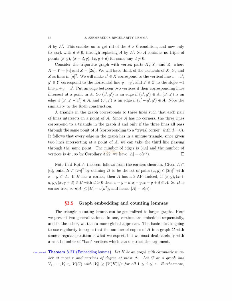
56 3. SZEMERÉDI’S REGULARITY LEMMA
A by A′. This enables us to get rid of the d > 0 condition, and now onlyto work with d 6= 0, through replacing A by A′. So A contains no triple ofpoints (x, y), (x+ d, y), (x, y + d) for some any d 6= 0.
Consider the tripartite graph with vertex parts X, Y , and Z, whereX = Y = [n] and Z = [2n]. We will have think of the elements of X, Y , andZ as lines in [n]2. We will make x′ ∈ X correspond to the vertical line x = x′,y′ ∈ Y correspond to the horizontal line y = y′, and z′ ∈ Z to the slope −1
line x+y = z′. Put an edge between two vertices if their corresponding linesintersect at a point in A. So (x′, y′) is an edge if (x′, y′) ∈ A, (x′, z′) is anedge if (x′, z′ − x′) ∈ A, and (y′, z′) is an edge if (z′ − y′, y′) ∈ A. Note thesimilarity to the Roth construction.
A triangle in the graph corresponds to three lines such that each pairof lines intersects in a point of A. Since A has no corners, the three linescorrespond to a triangle in the graph if and only if the three lines all passthrough the same point of A (corresponding to a “trivial corner” with d = 0).It follows that every edge in the graph lies in a unique triangle, since giventwo lines intersecting at a point of A, we can take the third line passingthrough the same point. The number of edges is 3|A| and the number ofvertices is 4n, so by Corollary
cor:TRL_corcor:TRL_cor3.22, we have |A| = o(n2).
Note that Roth’s theorem follows from the corners theorem. Given A ⊂[n], build B ⊂ [2n]2 by defining B to be the set of pairs (x, y) ∈ [2n]2 withx − y ∈ A. If B has a corner, then A has a 3-AP. Indeed, if (x, y), (x +
d, y), (x, y + d) ∈ B with d > 0 then x− y − d, x− y, x− y + d ∈ A. So B iscorner-free, so n|A| ≤ |B| = o(n2), and hence |A| = o(n).
§3.5 Graph embedding and counting lemmas
The triangle counting lemma can be generalized to larger graphs. Herewe present two generalizations. In one, vertices are embedded sequentially,and in the other, we take a more global approach. The basic idea is goingto use regularity to argue that the number of copies of H in a graph G withsome ε-regular partition is what we expect, but we must deal carefully witha small number of "bad" vertices which can obstruct the argument.
thm:embed Theorem 3.27 (Embedding lemma). Let H be an graph with chromatic num-ber at most r and vertices of degree at most ∆. Let G be a graph andV1, . . . , Vr ⊂ V (G) with |Vi| ≥ |V (H)|/ε for all 1 ≤ i ≤ r. Furthermore,
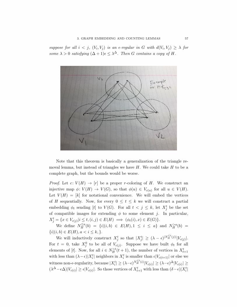
3. GRAPH EMBEDDING AND COUNTING LEMMAS 57
suppose for all i < j, (Vi, Vj) is an ε-regular in G with d(Vi, Vj) ≥ λ forsome λ > 0 satisfying (∆ + 1)ε ≤ λ∆. Then G contains a copy of H.
Note that this theorem is basically a generalization of the triangle re-moval lemma, but instead of triangles we have H. We could take H to be acomplete graph, but the bounds would be worse.
Proof. Let c : V (H) → [r] be a proper r-coloring of H. We construct aninjective map φ : V (H) → V (G), so that φ(u) ∈ Vc(u) for all u ∈ V (H).Let V (H) = [k] for notational convenience. We will embed the verticesof H sequentially. Now, for every 0 ≤ t ≤ k we will construct a partialembedding φt sending [t] to V (G). For all t < j ≤ k, let Xt
j be the setof compatible images for extending φ to some element j. In particular,Xtj = x ∈ Vc(j)|i ≤ t, (i, j) ∈ E(H) =⇒ (φt(i), x) ∈ E(G).We define N≤aH (b) = i|(i, b) ∈ E(H), 1 ≤ i ≤ a and N>a
H (b) =
i|(i, b) ∈ E(H), a < i ≤ k, .We will inductively construct Xt
j so that |Xtj | ≥ (λ − ε)|N
≤tH (j)||Vc(j)|.
For t = 0, take X0j to be all of Vc(j). Suppose we have built φt for all
elements of [t]. Now, for all i ∈ N>tH (t + 1), the number of vertices in Xt
t+1
with less than (λ−ε)|Xti | neighbors in Xt
i is smaller than ε|Vc(t+1)| or else wewitness non-ε-regularity, because |Xt
i | ≥ (λ−ε)N≤tH (i)|Vc(i)| ≥ (λ−ε)∆|Vc(i)| ≥(λ∆−ε∆)|Vc(i)| ≥ ε|Vc(i)|. So those vertices of Xt
t+1 with less than (δ−ε)|Xti |

58 3. SZEMERÉDI’S REGULARITY LEMMA
neighbors in Xti on one hand and Xt
i on the other hand would witness theirregularity for (Vc(t+1), Vc(i)).
Let m = |N≤tH (t + 1)|, the neighbors of t + 1 which are at most t. Theinductive hypothesis tells us that |Xt
t+1| ≥ (λ − ε)m|Vc(t+1)||. Eliminate,from Xt
t+1, the vertices with fewer than (λ − ε)|Xti | neighbors in Xt
i for alli ∈ N>t
H (t + 1). Note |N>tH (t + 1)| ≤ ∆ −m. So the remaining number of
vertices in Xtt+1 is at least
((λ− ε)m − (∆−m)ε)|Vc(t+1)| ≥ (λm −mε− (∆−m)ε)|Vc(t+1)|
≥ (λ∆ −∆ε)|Vc(t+1)| ≥ ε|Vc(t+1)| ≥ |V (H)|So we can pick a vertex of Vc(t+1) to define φt+1(t+ 1) (and define φt+1(i) =
φt(i) for i ≤ t), and φ is injective.It suffices to check that this new φt+1 has enough compatible images, i.e.
that |Xt+1j | ≥ (λ− ε)|N≤t+1
H (j)||Vc(j)| for any j > t+ 1. If (t+ 1, j) is not anedge of H, then
|Xt+1j | ≥ |Xt
j | ≥ (λ− ε)|N≤tH (j)||Vc(j)| = (λ− ε)|N
≤t+1H (j)||Vc(j)|
and we are done. If (t+ 1, j) ∈ E(H), then
|Xt+1j | ≥ (λ− ε)|Xt
j | ≥ (λ− ε)(λ− ε)|N≤tH (j)||Vc(j)| = (λ− ε)|N
≤t+1H (j)||Vc(j)|
and we are again done.
This version is good for graphs with low maximum degree, due to the(∆ + 1)ε ≤ λ∆ condition. When H is fairly dense and ∆ = Ω(|H|), thebound will be closer to the bound of a complete graph.
Recall that we defined a pair (X,Y ) to be ε-regular if |d(A,B)−d(X,Y )| ≤ε for all A ⊂ X, B ⊂ Y with |A| ≥ ε|X| and |B| ≥ ε|Y |. It will be convenientto introduce another notion which is almost equivalent to ε-regularity.
def:homog Definition 3.28. LetX,Y ⊂ V (G). We say that the pair (X,Y ) is ε-homogeneousif
|e(A,B)− d(X,Y )|A||B|| ≤ ε|X||Y | for all A ⊂ X and B ⊂ Y.
It turns out that this definition is equivalent up to a polynomial trans-formation in ε.

3. GRAPH EMBEDDING AND COUNTING LEMMAS 59
lem:reg-homog Lemma 3.29. Let ε > 0. In any graph, if a pair of vertex sets (X,Y ) is ε-regular, then it is ε-homogeneous. Conversely, if (X,Y ) is ε3-homogeneous,then it is ε-regular.
Proof. Suppose first that (X,Y ) is ε-regular. For every A ⊂ X and B ⊂ Y
we have |e(A,B)−d(X,Y )||A||B|| = |d(A,B)−d(X,Y )||A||B|. If |A| ≥ ε|X|and |B| ≥ ε|Y |, then by ε-regularity we have |d(A,B) − d(X,Y )||A||B| ≤ε|A||B| ≤ ε|X||Y |. Else, |d(A,B)−d(X,Y )||A||B| ≤ |A||B| ≤ ε|X||Y |. Thusthe pair (X,Y ) is ε-homogeneous.
Now, assume that a pair (X,Y ) is ε3-homogeneous. If A ⊂ X and B ⊂ Ysatisfies |A| ≥ ε|X| and |B| ≥ ε|Y |, then
|d(A,B)− d(X,Y )| = |e(A,B)− d(X,Y )|A||B|||A|B| ≤ ε3|X||Y |
ε|X|ε|Y | ≤ ε.
Thus (X,Y ) is ε-regular.
The notion of homogeneity enables us to more easily formulate a generalcounting lemma.
thm:counting Theorem 3.30 (Counting lemma). Let H be a graph with V (H) = [k]. LetG be a graph with Vi ⊂ V (G) for 1 ≤ i ≤ k so that (Vi, Vj) is ε-homogeneousfor all ij ∈ E(H). Let N(H) denote the number of homomorphisms H → G
where each i ∈ V (H) is mapped into Vi, i.e.,
N(H) := |(v1, · · · , vk) ∈ V1×· · ·×Vk : (vi, vj) ∈ E(G) for all (i, j) ∈ E(H)|.
Then ∣∣∣∣∣∣N(H)−∏
ij∈E(H)
d(Vi, Vj) ·k∏i=1
|Vi|
∣∣∣∣∣∣ ≤ |E(H)|εk∏i=1
|Vi|
Note that the Vi’s do not have to be disjoint. The quantityN(H) includesnon-injective maps V (H)→ V (G), but since the a negligible fraction of suchmaps are non-injective (for fixedH and large |V (G)|), we can use the theoremto find a genuine copy of H in G.
Proof. The proof proceeds by induction on |E(H)|. The result is trivialfor empty graphs since N(H) =
∏ki=1 |Vi| if H is empty. Without loss of
generality, suppose (1, 2) ∈ E(H). Let H ′ be H without the edge (1, 2).Suppose we fix v = (v3, · · · , vk) ∈ V3 × · · · × Vk. Let X1(v) be the setof v1 ∈ V1 such that (v1, vi) ∈ E(G) whenever (1, i) ∈ E(H). Define X2(v)

60 3. SZEMERÉDI’S REGULARITY LEMMA
similarly. We say that v is valid if for any 3 ≤ i < j ≤ k whenever (i, j) ∈ H,(vi, vj) ∈ G.
Then,N(H) =
∑valid v∈V3×···×Vk
eG(X1(v), X2(v))
andN(H ′) =
∑v
|X1(v)||X2(v)|.
So |N(H) − N(H ′)d(V1, V2)| ≤ ε∏ki=1 |Vi| by ε-homogeneity, because the
difference is at most ε|V1||V2| for each of the at most∏ki=3 |Vi| choices of v.
We have∣∣∣∣∣∣N(H)−∏
ij∈E(H)
d(Vi, Vj) ·k∏i=1
|Vi|
∣∣∣∣∣∣≤∣∣N(H)−N(H ′)d(V1, V2)
∣∣+ d(V1, V2)
∣∣∣∣∣∣N(H ′)−∏
ij∈E(H′)
d(Vi, Vj) ·k∏i=1
|Vi|
∣∣∣∣∣∣≤ ε
k∏i=1
|Vi|+ |E(H ′)|εk∏i=1
|Vi|
= |E(H)|εk∏i=1
|Vi|.
Thus, the induction is complete.
Lec9: MatthewBrennan
The following removal lemma for general graphs follows from the sameproof as the triangle removal lemma.
thm:graph-removal Theorem 3.31 (Graph removal lemma). For all H and ε > 0, there is a δ > 0
such that if G has n vertices and at most δn|V (H)| copies of H, then G canbe made H-free by removing at most εn2 edges.
§3.6 Another proof of Erdős-Stone-Simonovits theorem
Now we give an alternative proof of Erdős-Stone-Simonovits theorem,Theorem
thm:essthm:ess2.14. Recall it says that for a fixed graph H,
ex(n,H) =
(1− 1
χ(H)− 1+ o(1)
)n2
2as n→∞.
We will use Szemerédi’s regularity lemma and the counting lemma. Theproof will again follow our general recipe for applying the regularity lemma:

3. ANOTHER PROOF OF ERDŐS-STONE-SIMONOVITS THEOREM 61
(1) (Partition) Find a regular partition(2) (Clean) Remove edges between irregular, low-density and from small
vertex sets(3) (Count) Find a structure in the in the “reduced graph" and apply
the counting lemma
Proof. Let χ(H) = r + 1 and let ε > 0. Suppose G has n vertices and atleast
|E(G)| ≥(
1− 1
χ(H)− 1+ ε
)n2
2
edges. We will show that if n is sufficiently large, the graph G contains a copyof H. Applying Szemerédi’s regularity lemma, let V (G) = V1]V2] · · ·]VMbe an ε′-regular partition where ε′ is to be chosen later. Now remove eachedge (x, y) of G if
(1) (x, y) ∈ Vi × Vj where (Vi, Vj) is not ε-regular(2) (x, y) ∈ Vi × Vj where d(Vi, Vj) <
ε8
(3) x ∈ Vi where |Vi| < εn4M
The number of edges removed is at most εn2/8 in each step and thus at most3εn2/8 edges in total are removed. After removing those edges, the resultinggraph G′ has at least (
1− 1
χ(H)− 1+ε
4
)n2
2
edges. By Turán’s theorem, G′ contains a copy of Kr+1. Let the verticesof this copy of Kr+1 lie in Vi1 , Vi2 , . . . , Vir+1 , allowing some of the indices tocoincide. By the counting lemma,(
#homomorphisms H → G′)≥[( ε
8
)|E(H)|− |E(H)|ε′
] ∏v∈H|Viϕ(v)
|
≥[( ε
8
)|E(H)|− |E(H)|ε′
] ∏v∈H
( εn4M
)|V (H)|
where ϕ : H → [r] is a coloring. If we set ε′ = 12|E(H)|
(ε8
)|E(H)|, then(#homomorphisms H → G′
)≥ cn|V (H)|
for some constant c > 0 depending on ε and H. Since the number of non-injective homomorphisms is OH(n|V (H)|−1), for sufficiently large n, G mustcontain a genuine copy of H with distinct vertices.

62 3. SZEMERÉDI’S REGULARITY LEMMA
The intuition in this proof is that the counting lemma yields a method to“boost” a copy ofKr+1 guaranteed by Turán’s theorem to a more complicatedgraph H. We remark that the phenomenon where above the threshold onecopy leads to many copies of a graph H is called “supersaturation”.
§3.7 Hypergraph removal lemma and Szemerédi’s theorem
Szemerédi’s regularity lemma can also be generalized to hold for hyper-graphs. However, it is difficult to formalize this lemma and to prove it. Oneuseful application is the hypergraph removal lemma, which we will now stateand use to prove Szemerédi’s Theorem. To review, an r-uniform hypergraphG has vertex set V (G) and edge set E(G) which consists of a collection ofr-element subsets of V (G).
thm:hypergraph-removal Theorem 3.32 (Hypergraph removal lemma). For all r-uniform hypergraphsH and ε > 0, there is a δ > 0 such that if G is an r-uniform hypergraph withn vertices and at most δn|V (H)| copies of H, then G can be made H-free byremoving εnr hyperedges.
cor:hypergraph-cor Corollary 3.33. Fix an r-uniform hypergraph H with |E(H)| > 1. If G is anr-uniform hypergraph on n vertices where every hyperedge is contained in aunique copy of H, then G has G has o(nr) hyperedges.
This corollary follows from a similar argument to the corollary of thetriangle removal lemma. The number of copies of H is o(n|V (H)|) and thusremoving e = o(nr) edges renders the hypergraph H-free. However, there areat most e · |E(H)| edges in G since each hyperedge is contained in a uniquecopy of H. We will use this corollary to deduce Szemerédi’s Theorem.
thm:szemeredi Theorem 3.34 (Szemerédi’s theorem). Fix any k ≥ 3. Any k-AP-free setA ⊆ [N ] has |A| = o(N).
We will illustrate the proof for k = 4, and it will be obvious how toextend this proof to all values of k. Here a tetrahedron consists of edgescorresponding to all possible 3-element subsets of a 4-element set.
Proof. Let m be the smallest integer larger than 4n and coprime to 6. Weremark that this is to avoid wrap-around and divisibility issues. We embedin Z/mZ. This bound on m ensures that 4-APs in A are the same viewedin Z as in Z/mZ. We will build a 3-uniform 4-partite hypergraph G such

3. HYPERGRAPH REMOVAL LEMMA AND SZEMERÉDI’S THEOREM 63
that the 4-AP’s in A correspond to tetrahedra in G. The four parts will beX,Y, Z and W all of which are copies of Z/mZ. Given x ∈ X, y ∈ Y, z ∈ Zand w ∈W , we insert an edges as follows:
• (x, y, z) ∈ E(G) if and only if 3x+ 2y + z ∈ A;• (x, y, w) ∈ E(G) if and only if 2x+ y − w ∈ A;• (x, z, w) ∈ E(G) if and only if x− z − 2w ∈ A;• (y, z, w) ∈ E(G) if and only if −y − 2z − 3w ∈ A.
Note that 4-APs correspond to tetrahedra because (x, y, z, w) is a tetrahe-dron if and only if all four expressions lie in A. But then the expressionsform a 4-AP with common difference −x− y − z −w. Since A is 4-AP-free,this is possible if and only if x + y + z + w = 0. Thus every hyperedgelies in a unique tetrahedron since (x, y, z) can be uniquely completed to atetrahedron with vertex w = −x − y − z. By Corollary
cor:hypergraph-corcor:hypergraph-cor3.33, we have that
|E(G)| = o(n3). Now note that |E(G)| = 4m2|A|. Since m > 4n, we havethat |A| = o(n).
We remark that m is coprime to 6 in order to avoid issues with thenumber of the solutions to equations such as x + 2y + 3w = a. We nowgive some intuition. Loosely, the “complexity" of patterns depends on howmany equations they arise from. If they arise from one equation, often graphtheory or Fourier analysis is enough. If patterns are described by two or moreequations, we often have apply analogous theorems involving hypergraphs.Also, Fourier analysis often stops working and we require quadratic Fourieranalysis, which was introduced by Gowers. The ergodic theory approachesalso display a parallel hierarchy structure.
We now state some bounds. Each step up in r-uniformity requires astep up in the Ackerman hierarchy. The requirement for the 3-uniform hy-pergraph regularity lemma is wowzer(ε−O(1)), which is the tower functioniterated ε−O(1) times (similar to how the tower function is iterated exponen-tials). It was proven by Gowers with higher-order Fourier analysis that themaximum size rk(N) of a subset of [N ] avoiding k-AP’s satisfies
rk(N) ≤ O(
N
(log logN)ck
).
The best known lower bound is not so much better than Behrend’s boundN
e(logN)c′k≤ rk(N).

64 3. SZEMERÉDI’S REGULARITY LEMMA
For 4-APs, Green-Tao showed a slightly better bound of
r4(N) ≤ O(
N
(logN)c
)for some constant c > 0. Recall for r3(N), we know that this bound holdswith c = 1 + o(1).
CHAPTER 4
Pseudorandom graphsch:pseudorandom-graphs
§4.1 Eigenvalues
In this chapter, we will discuss graphs that “look random” in some sense,and compare the different ways that a graph can be random-like.
We first review some basic facts in spectral graph theory. The adjacencymatrix of a graph G = (V,E) with V = v1, v2, . . . , vn is an n × n matrixA where
aij =
1 if (vi, vj) ∈ E,0 otherwise.
It is symmetric and therefore diagonalizable. Therefore:
• There are n real eigenvalues λ1 ≥ λ2 ≥ · · · ≥ λn• There is an orthonormal basis of eigenvectors v1, v2, . . . , vn ∈ Rn
where it holds that
Avi = λivi and A =
n∑i=1
λivivti .
If G is d-regular (i.e. deg(v) = d for all v ∈ V (G)) then d = λ1 ≥ λ2 ≥ · · · ≥λn ≥ −d and v1 is the all ones vector. Some facts:
• If G is connected, then λ2 < d.
• G is bipartite if and only if λn = −d (bipartite in general impliesλi = −λn−i, as vi can be obtained from vi−1 by negating the coor-dinates corresponding to one of the two vertex parts).
We first prove the following lemma about d-regular graphs, which is ina sense a stronger notion of ε-regularity since it also holds for small sets Xand Y .
thm:eml Theorem 4.1 (Expander mixing lemma). Let G be a d-regular graph with n
vertices. Let λ1 ≥ λ2 ≥ · · · ≥ λn be the eigenvalues of the adjacency matrix
65

66 4. PSEUDORANDOM GRAPHS
and let λ = max|λ2|, |λn|. Then for all X,Y ⊆ V (G),∣∣∣∣e(X,Y )− d
n|X||Y |
∣∣∣∣ ≤ λ√|X||Y |.Proof. Let A be the adjacency matrix of G and J be the n×n all 1’s matrix.It turns out that A − d
nJ has the same eigenvectors as A. We check this.Note that v1 = 1 (the all 1’s n× 1 vector) and thus(
A− d
nJ
)1 = 0.
For all 2 ≤ i ≤ n, since 〈vi,1〉 = 0 due to orthogonality of eigenvectors (andconsequently Jvi = 0), we have that(
A− d
nJ
)vi = λivi.
So A− dnJ has eigenvalues 0, λ2, λ3, . . . , λn. Thus its spectral norm is λ. The
spectral norm ‖B‖ for symmetric matrices B satisfies a Rayleigh quotient oroperator norm identity
‖B‖ = supu,v 6=0
utBv
|u| · |v| .
Let 1X be the n × 1 vector with 1’s at entries numbered by vertices ofsubgraph X, and 0’s everywhere else. Note that∣∣∣∣e(X,Y )− d
n|X||Y |
∣∣∣∣ =
∣∣∣∣1tX (A− d
nJ
)1Y
∣∣∣∣≤ |1X | · |1Y | ·
∥∥∥∥A− d
nJ
∥∥∥∥≤ λ
√|X||Y |.
Lec10: Hong Wang
Remark 4.2. (a) Expander mixing lemma is stronger than the notion of ε–regularity since X and Y could be smaller than linear size.
(b) For d–regular bipartite graphs, λi = −λn+1−i, one should replace λby λ2 and restrict X, Y to different parts of the bipartition.
Bilu and Linial showed that the converse to Expander mixing lemmaholds as well.
Theorem 4.3 (Converse to expander mixing lemma). Let G be a d–regulargraph on n vertices whose adjacency matrix has eigenvalues λ1 ≥ λ2 ≥ · · · ≥

4. EIGENVALUES 67
λn. If
|e(X,Y )− d
n|X||Y || ≤ β
√|X||Y |
for any X,Y ⊆ V (G), then
max|λ2|, |λn| = O(β(1 + logd
β)).
This theorem is tight.Random graphs mix well. The following result can be proved by bound-
ing eigenvalues. We omit the proof.
Theorem 4.4. Let p = p(n) ≤ 0.99, with probability 1 − o(1), the randomgraph G(n, p) satisfies
|e(X,Y )− p|X||Y || = O(√pn|X||Y |)
for any X,Y ⊆ V (G).
We might have different interpretations of d, sometimes we think of das a constant and let n approach infinity; sometimes we think of d as thedegree of a dense graph.
The following theorem is a very difficult result. Its proof is over 100pages long!
Theorem 4.5 (Friedman’s second eigenvalue theorem). Fix d ≥ 3, with proba-bility 1− o(1) as n→∞, a random d–regular graph on n vertices has all butthe top eigenvalue bounded in absolute value by 2
√d− 1+o(1), with o(1)→ 0
as n→∞.
The above bound is nearly best possible, due to the next result (whichhas a short neat proof, which unfortunately we will not cover).
Theorem 4.6 (Alon-Boppana). For fixed d, the second largest eigenvalue λ2
of the adjacency matrix of a d-regular graph satisfies λ2 ≥ 2√d− 1 − o(1),
where o(1) goes to zero as the number of vertices goes to infinity.
Definition 4.7. Ramanujan Graphs are d–regular graphs with |λ2|, |λn| ≤2√d− 1.
The bound 2√d− 1 is natural due to Friedman’s second eigenvalue the-
orem and Alon-Boppana theorem. A more intricate explanation for why
68 4. PSEUDORANDOM GRAPHS
2√d− 1 is important is that it is the spectral radius of the infinite d-regular
tree, which is the universal cover for all d-regular graphs.It remains a major open problem to find Ramanujan graphs.
Conjecture 4.8. For any d ≥ 3, there exists infinitely many d–regular Ra-manujan graphs.
In 1987, Lubotzky, Phillips and Sanark proved the conjecture whend = p + 1 for prime p ≡ 1 (mod 4) using deep tools from number theoryrelated to the Ramanujan conjecture (hence the name Ramanujan graphs).Morgenstern generalized this result to d = q + 1 where q is a prime power.
In 2013, Marcus, Spielman, and Srivastava devised an elegant probabilis-tic construction for bipartite Ramanujan graphs (where we simply requireλ2 ≤ 2
√d− 1, noting that λi = −λn−i). They showed that for any d ≥ 3,
there exists infinitely many bipartite d–regular Ramanujan graphs.
§4.2 Fourier analysis on finite abelian groups
A important class of constructions for pseudorandom graphs are Cayleygraphs, arising from groups.
Definition 4.9 (Cayley Graph). Let Γ be a finite group and S is a subset ofΓ such that S−1 = S. The Cayley Graph Cay(Γ, S) has vertices Γ, edges(g, gs) for any g ∈ Γ and s ∈ S.
We will mostly work with abelian groups, in which case we use additivenotation.
Definition 4.10 (Paley graph). A Paley graph of order p is defined as Cay(Z/pZ, S)
with prime p ≡ 1 (mod 4). Here S ⊂ Z/pZ consists of the non-zero qua-dratic residues.
We will show that the second largest eigenvalue bound for Paley graphis O(
√p).
Definition 4.11. Given an abelian group Γ, a character is a homomorphismχ : Γ → C× = (z ∈ C, z 6= 0,×). In other words, χ satisfies χ(a)χ(b) =
χ(a+ b) for any a, b ∈ Γ.
For finite groups, we have
χ(a)|Γ| = χ(|Γ|a) = χ(0) = 1.
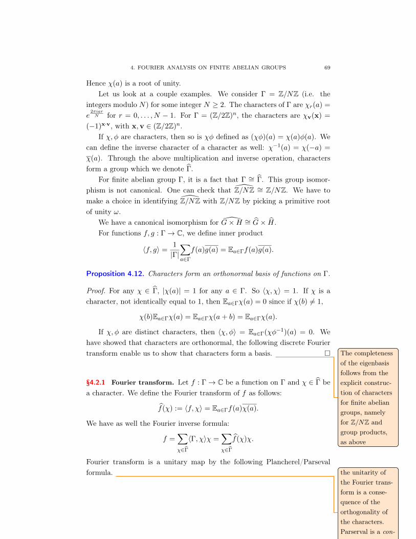
4. FOURIER ANALYSIS ON FINITE ABELIAN GROUPS 69
Hence χ(a) is a root of unity.Let us look at a couple examples. We consider Γ = Z/NZ (i.e. the
integers modulo N) for some integer N ≥ 2. The characters of Γ are χr(a) =
e2πiarN for r = 0, . . . , N − 1. For Γ = (Z/2Z)n, the characters are χv(x) =
(−1)x·v, with x,v ∈ (Z/2Z)n.If χ, φ are characters, then so is χφ defined as (χφ)(a) = χ(a)φ(a). We
can define the inverse character of a character as well: χ−1(a) = χ(−a) =
χ(a). Through the above multiplication and inverse operation, charactersform a group which we denote Γ.
For finite abelian group Γ, it is a fact that Γ ∼= Γ. This group isomor-phism is not canonical. One can check that Z/NZ ∼= Z/NZ. We have tomake a choice in identifying Z/NZ with Z/NZ by picking a primitive rootof unity ω.
We have a canonical isomorphism for G×H ∼= G× H.For functions f, g : Γ→ C, we define inner product
〈f, g〉 =1
|Γ|∑a∈Γ
f(a)g(a) = Ea∈Γf(a)g(a).
Proposition 4.12. Characters form an orthonormal basis of functions on Γ.
Proof. For any χ ∈ Γ, |χ(a)| = 1 for any a ∈ Γ. So 〈χ, χ〉 = 1. If χ is acharacter, not identically equal to 1, then Ea∈Γχ(a) = 0 since if χ(b) 6= 1,
χ(b)Ea∈Γχ(a) = Ea∈Γχ(a+ b) = Ea∈Γχ(a).
If χ, φ are distinct characters, then 〈χ, φ〉 = Ea∈Γ(χφ−1)(a) = 0. Wehave showed that characters are orthonormal, the following discrete Fouriertransform enable us to show that characters form a basis. The completeness
of the eigenbasisfollows from theexplicit construc-tion of charactersfor finite abeliangroups, namelyfor Z/NZ andgroup products,as above
The completenessof the eigenbasisfollows from theexplicit construc-tion of charactersfor finite abeliangroups, namelyfor Z/NZ andgroup products,as above
§4.2.1 Fourier transform. Let f : Γ→ C be a function on Γ and χ ∈ Γ bea character. We define the Fourier transform of f as follows:
f(χ) := 〈f, χ〉 = Ea∈Γf(a)χ(a).
We have as well the Fourier inverse formula:
f =∑χ∈Γ
〈Γ, χ〉χ =∑χ∈Γ
f(χ)χ.
Fourier transform is a unitary map by the following Plancherel/Parsevalformula. the unitarity of
the Fourier trans-form is a conse-quence of theorthogonality ofthe characters.Parserval is a con-sequence of uni-tarity
the unitarity ofthe Fourier trans-form is a conse-quence of theorthogonality ofthe characters.Parserval is a con-sequence of uni-tarity

70 4. PSEUDORANDOM GRAPHS
Theorem 4.13 (Plancherel/Parseval’s theorem). 〈f, g〉 =∑χ∈Γ
f(χ)g(χ).
Proof.
〈f, g〉 = 〈∑χ∈Γ
f(χ)χ,∑φ∈Γ
g(φ)φ〉
=∑χ,φ∈Γ
f(χ)g(φ)〈χ, φ〉
=∑χ∈Γ
f(χ)g(χ)〈χ, χ〉
We calculate the Fourier transform for a couple examples.When Γ is the Cyclic group Z/NZ,
f(χr) = f(r) =1
N
∑a∈Z/NZ
f(a)e−2πiarN .
We can write f as f(a) =∑N−1
r=0 f(r)e2πiarN .
When Γ is the Boolean cube (Z/2Z)n,
f(χv) = f(v) =1
2n
∑a∈(Z/2Z)n
f(a)(−1)v·a.
In particular, the characters of Boolean cube are real valued.Here are some more classic examples with non-finite abelian groups.
When Γ is a circle Γ = R/Z, Γ ∼= Z (Note that Γ Γ). We have theFourier series:
f(n) =
∫R/Z
f(x)e−2πinxdx,
f(x) =∑n∈Z
f(n)e2πinx.
When Γ is the real line Γ = R, Γ ∼= R. We have the usual Fourier transform:
f(ξ) =
∫ +∞
−∞f(x)e−2πixξdx,
f(x) =
∫ +∞
−∞f(ξ)e2πixξdξ.
Proposition 4.14. Let Γ be a finite abelian group, S ⊂ Γ\0 is a multiplica-tive subset such that S = S−1. Let A be the adjacency matrix of Cay(Γ, S),

4. QUASIRANDOM GRAPHS 71
for any χ ∈ Γ,(χ(a)
)a∈Γ
is an eigenvector of A with eigenvalue∑
s∈S χ(s).In particular, this is a complete basis of eigenvectors of A.
The proposition is an immediate corollary of the following lemma.
Lemma 4.15. If f : Γ→ C is a function on Γ and let A be a |Γ|×|Γ| complexmatrix defined by Aa,b = f(b − a), then χ ∈ Γ,
(χ(a)
)a∈Γ
is an eigenvectorof A with eigenvalue |Γ|f(χ).
Proof. Let x =(χ(a)
)a∈Γ
.
(Ax)a =∑b∈Γ
Aa,bχ(b)
=∑b
f(b− a)χ(b) =∑b
f(b− a)χ(b− a)χ(a)
= f(χ)χ(a)|Γ|
We summarize the connection as: the eigenvalues of the graphs have oneto one correspondence with the Fourier transform of 1S .
§4.2.2 Paley graph.
Proposition 4.16. Let p ≡ 1 (mod 4) be a prime. The Paley graph Cay(Z/pZ, S),where S is the collection of non-zero quadratic residues. In particular, |S| =p−1
2 is the degree of the Paley graph. If eigenvalues λ1 ≥ λ2 ≥ · · · ≥ λn, thenmax|λ2|, |λn| =
√p+12 .
Proof. Let χ be a non-trivial character. 1 + 2∑
s∈S χ(s) =∑
a∈Z/pZχ(a2). We
calculate the Gauss-Sum:
|∑a
χ(a2)|2 =∑a,b
χ((a+ b)2)χ(a2)
=∑a,b
χ((a+ b)2 − a2) =∑a,b
χ(2ab+ b2) = |Γ| = p
Thus∑
s∈S χ(s) =±√p−1
2 .
§4.3 Quasirandom graphs
Lec11: Linus Hamilton(IN PROGRESS)
The following theorem consolidates many notions of “randomness” we’veseen so far.
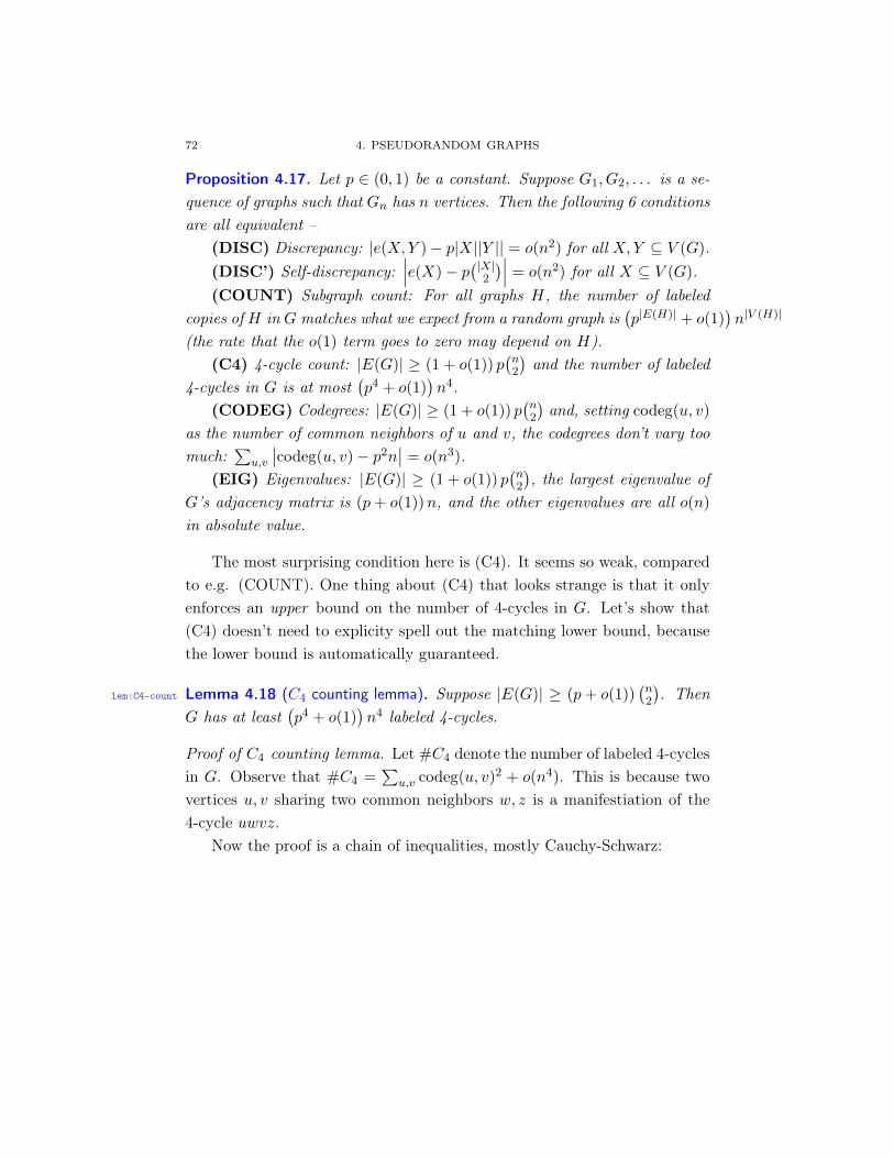
72 4. PSEUDORANDOM GRAPHS
Proposition 4.17. Let p ∈ (0, 1) be a constant. Suppose G1, G2, . . . is a se-quence of graphs such that Gn has n vertices. Then the following 6 conditionsare all equivalent –
(DISC) Discrepancy: |e(X,Y )− p|X||Y || = o(n2) for all X,Y ⊆ V (G).(DISC’) Self-discrepancy:
∣∣∣e(X)− p(|X|
2
)∣∣∣ = o(n2) for all X ⊆ V (G).(COUNT) Subgraph count: For all graphs H, the number of labeled
copies of H in G matches what we expect from a random graph is(p|E(H)| + o(1)
)n|V (H)|
(the rate that the o(1) term goes to zero may depend on H).(C4) 4-cycle count: |E(G)| ≥ (1 + o(1)) p
(n2
)and the number of labeled
4-cycles in G is at most(p4 + o(1)
)n4.
(CODEG) Codegrees: |E(G)| ≥ (1 + o(1)) p(n2
)and, setting codeg(u, v)
as the number of common neighbors of u and v, the codegrees don’t vary toomuch:
∑u,v
∣∣codeg(u, v)− p2n∣∣ = o(n3).
(EIG) Eigenvalues: |E(G)| ≥ (1 + o(1)) p(n2
), the largest eigenvalue of
G’s adjacency matrix is (p+ o(1))n, and the other eigenvalues are all o(n)
in absolute value.
The most surprising condition here is (C4). It seems so weak, comparedto e.g. (COUNT). One thing about (C4) that looks strange is that it onlyenforces an upper bound on the number of 4-cycles in G. Let’s show that(C4) doesn’t need to explicity spell out the matching lower bound, becausethe lower bound is automatically guaranteed.
lem:C4-count Lemma 4.18 (C4 counting lemma). Suppose |E(G)| ≥ (p+ o(1))(n2
). Then
G has at least(p4 + o(1)
)n4 labeled 4-cycles.
Proof of C4 counting lemma. Let #C4 denote the number of labeled 4-cyclesin G. Observe that #C4 =
∑u,v codeg(u, v)2 + o(n4). This is because two
vertices u, v sharing two common neighbors w, z is a manifestiation of the4-cycle uwvz.
Now the proof is a chain of inequalities, mostly Cauchy-Schwarz:

4. QUASIRANDOM GRAPHS 73
#C4 =∑u,v
codeg(u, v)2 + o(n4)
≥ 1
n2
(∑u,v
codeg(u, v)
)2
+ o(n4) (Cauchy-Schwarz)
=1
n2
(∑u
deg(u)2
)2
+ o(n4)
≥ 1
n2
1
n
(∑u
deg(u)
)22
+ o(n4) (Cauchy-Schwarz)
=(p4 + o(1)
)n4
as desired.
Now let’s start proving that the 6 quasirandomness conditions are equiv-alent to each other. We’ll prove one implication at a time.
(DISC) ⇔ (DISC’)
Proof of (DISC) ⇔ (DISC’). Since (DISC’) is a subcase of (DISC), it suf-fices to show that (DISC’) implies (DISC).
This is true because e(X,Y ) = e(X∪Y )+e(X∩Y )−e(X\Y )−e(Y \X).If all the quantities on the right-hand side are approximately what we expectfrom a random graph (plus o(n2) error), then so is the left-hand side.
(DISC) =⇒ (COUNT) This is the counting lemma.(COUNT) =⇒ (C4) Obvious.(C4) =⇒ (CODEG)
Proof of (C4) =⇒ (CODEG). Suppose (C4) holds. We’ll prove (CODEG)using an inequality chain. The first inequality is Cauchy-Schwarz. We’ll use#C4 to denote the number of labeled 4-cycles in G.

74 4. PSEUDORANDOM GRAPHS
∑u,v
∣∣codeg(u, v)− p2n∣∣ ≤ n
(∑u,v
(codeg(u, v)− p2n
)2)1/2
= n
(∑u,v
codeg(u, v)2 − 2p2n∑u,v
codeg(u, v) + p4n4
)1/2
(Expand)
≤ n
(#C4 − 2p2n
∑v
deg(v)2 + p4n4 + o(n4)
)1/2
≤ n(#C4 − 2p4n4 + p4n4 + o(n4)
)1/2 (Jensen’s and |E(G)| bound)
≤ n(p4n4 − 2p4n4 + p4n4 + o(n4)
)1/2 ((C4) condition)
= o(n3)
as desired.
(CODEG) =⇒ (DISC)
Proof of (CODEG) =⇒ (DISC). Again, the proof is a chain of inequalities,using Cauchy-Schwarz. Assume (CODEG) holds. We’ll first prove as alemma that the vertex degrees don’t vary too much: to be precise, we’llprove
∑u | deg(u)− pn| = o(n2).
∑u
|deg(u)− pn| ≤ n1/2
(∑u
(deg(u)− pn)2
)1/2
= n1/2
(∑u
deg(u)2 − pn∑u
deg(u) + p2n2
)1/2
(Expand)
= n1/2
(∑u,v
codeg(u, v)− p2n2 + o(n3)
)1/2
= o(n2) (Use (CODEG))
as desired. Now, we can use (CODEG) to prove the inequality (DISC).
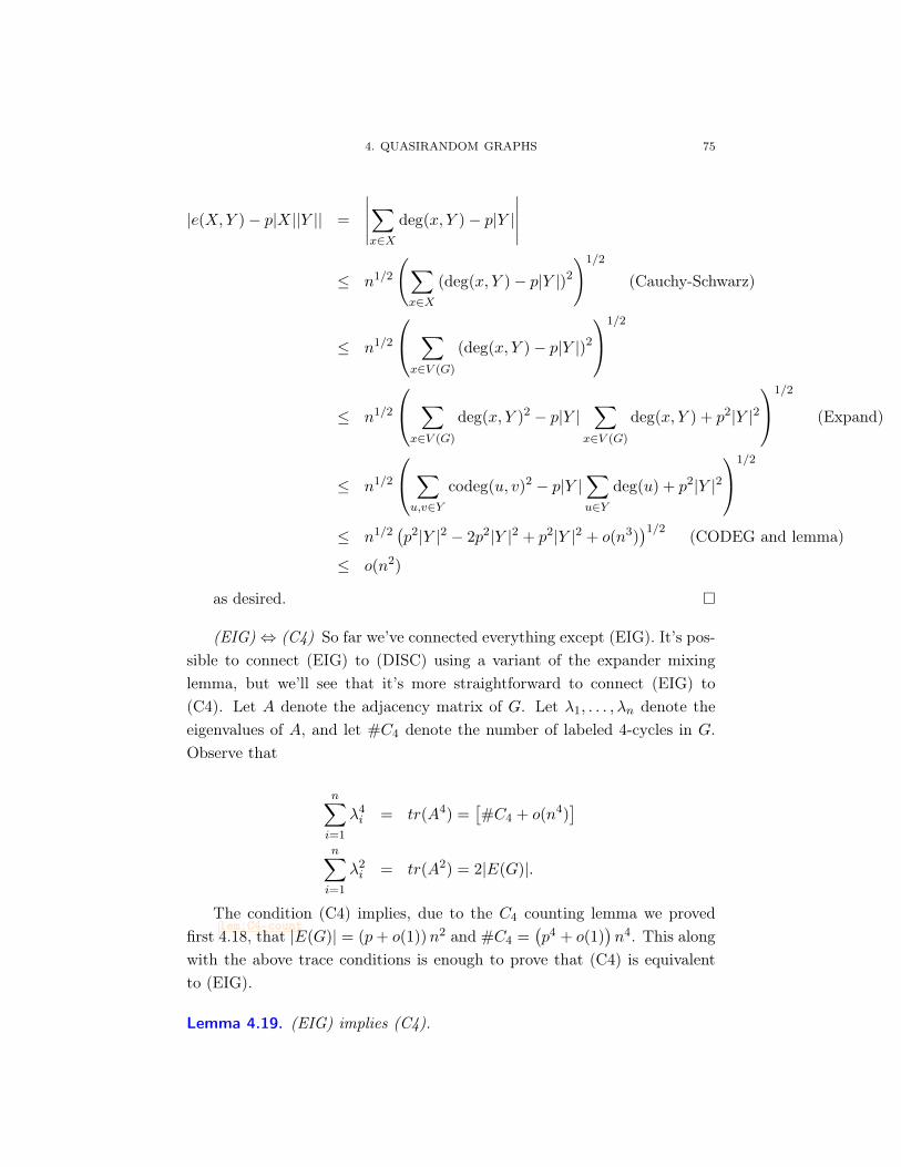
4. QUASIRANDOM GRAPHS 75
|e(X,Y )− p|X||Y || =
∣∣∣∣∣∑x∈X
deg(x, Y )− p|Y |∣∣∣∣∣
≤ n1/2
(∑x∈X
(deg(x, Y )− p|Y |)2
)1/2
(Cauchy-Schwarz)
≤ n1/2
∑x∈V (G)
(deg(x, Y )− p|Y |)2
1/2
≤ n1/2
∑x∈V (G)
deg(x, Y )2 − p|Y |∑
x∈V (G)
deg(x, Y ) + p2|Y |21/2
(Expand)
≤ n1/2
∑u,v∈Y
codeg(u, v)2 − p|Y |∑u∈Y
deg(u) + p2|Y |21/2
≤ n1/2(p2|Y |2 − 2p2|Y |2 + p2|Y |2 + o(n3)
)1/2 (CODEG and lemma)
≤ o(n2)
as desired.
(EIG)⇔ (C4) So far we’ve connected everything except (EIG). It’s pos-sible to connect (EIG) to (DISC) using a variant of the expander mixinglemma, but we’ll see that it’s more straightforward to connect (EIG) to(C4). Let A denote the adjacency matrix of G. Let λ1, . . . , λn denote theeigenvalues of A, and let #C4 denote the number of labeled 4-cycles in G.Observe that
n∑i=1
λ4i = tr(A4) =
[#C4 + o(n4)
]n∑i=1
λ2i = tr(A2) = 2|E(G)|.
The condition (C4) implies, due to the C4 counting lemma we provedfirst
lem:C4-countlem:C4-count4.18, that |E(G)| = (p+ o(1))n2 and #C4 =
(p4 + o(1)
)n4. This along
with the above trace conditions is enough to prove that (C4) is equivalentto (EIG).
Lemma 4.19. (EIG) implies (C4).
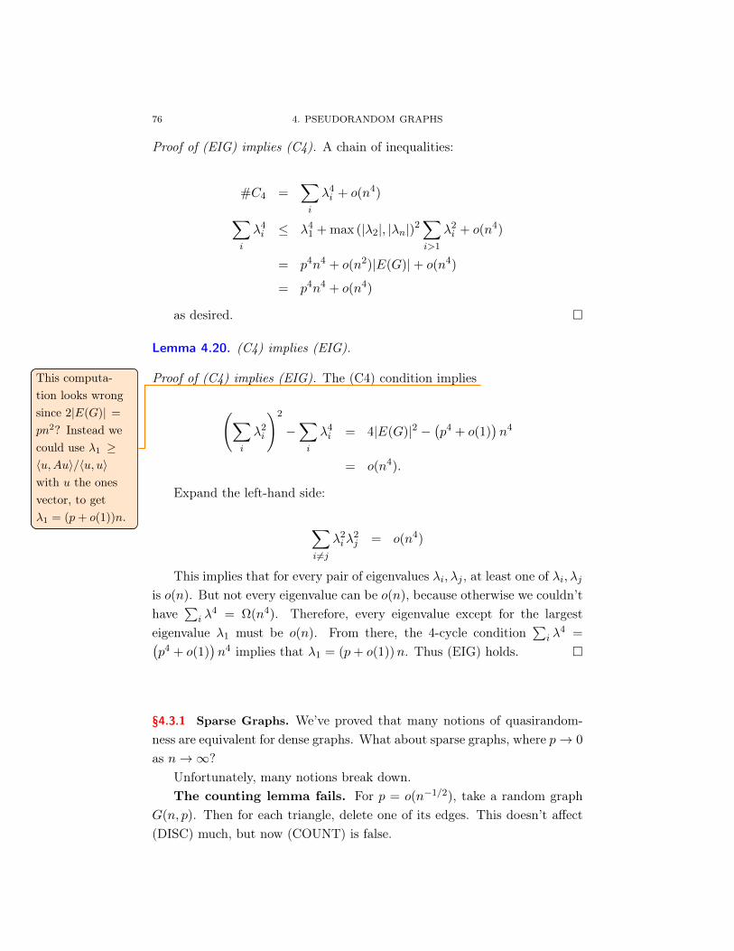
76 4. PSEUDORANDOM GRAPHS
Proof of (EIG) implies (C4). A chain of inequalities:
#C4 =∑i
λ4i + o(n4)∑
i
λ4i ≤ λ4
1 + max (|λ2|, |λn|)2∑i>1
λ2i + o(n4)
= p4n4 + o(n2)|E(G)|+ o(n4)
= p4n4 + o(n4)
as desired.
Lemma 4.20. (C4) implies (EIG).
Proof of (C4) implies (EIG). The (C4) condition impliesThis computa-tion looks wrongsince 2|E(G)| =
pn2? Instead wecould use λ1 ≥〈u,Au〉/〈u, u〉with u the onesvector, to getλ1 = (p+ o(1))n.
This computa-tion looks wrongsince 2|E(G)| =
pn2? Instead wecould use λ1 ≥〈u,Au〉/〈u, u〉with u the onesvector, to getλ1 = (p+ o(1))n.
(∑i
λ2i
)2
−∑i
λ4i = 4|E(G)|2 −
(p4 + o(1)
)n4
= o(n4).
Expand the left-hand side:
∑i 6=j
λ2iλ
2j = o(n4)
This implies that for every pair of eigenvalues λi, λj , at least one of λi, λjis o(n). But not every eigenvalue can be o(n), because otherwise we couldn’thave
∑i λ
4 = Ω(n4). Therefore, every eigenvalue except for the largesteigenvalue λ1 must be o(n). From there, the 4-cycle condition
∑i λ
4 =(p4 + o(1)
)n4 implies that λ1 = (p+ o(1))n. Thus (EIG) holds.
§4.3.1 Sparse Graphs. We’ve proved that many notions of quasirandom-ness are equivalent for dense graphs. What about sparse graphs, where p→ 0
as n→∞?Unfortunately, many notions break down.The counting lemma fails. For p = o(n−1/2), take a random graph
G(n, p). Then for each triangle, delete one of its edges. This doesn’t affect(DISC) much, but now (COUNT) is false.

4. QUASIRANDOM GRAPHS 77
(DISC) =⇒ (EIG) fails. Take G(n, p) plus a disjoint clique Kbpnc.If p is small, the new clique doesn’t add enough vertices to affect (DISC),but it creates a new large eigenvalue.
Some implications still work, though.(C4) =⇒ (CODEG) =⇒ (DISC) still works, as does (C4) =⇒
(EIG) =⇒ (DISC), as long as (DISC)’s bound is changed from o(n2) too(pn2).
In sparse settings, we need extra hypotheses for pseudorandomness. Lec12: YonahBorns-Weil and MattBabbitt
Although the properties of pseudorandomness are not true in general forsparse graphs, in the case of Cayley graphs we can still state a meaning-ful result. Intuitively, this is because Cayley graphs hold some symmetryproperties, which prevent a small clique from giving a large eigenvalue.
To make our result explicit, define the following properties of a d-regulargraph G:
• DISC(ε) means∣∣e(X,Y )− d
n |X||Y |∣∣ ≤ εdn for all X,Y ⊆ V (G).
• EIG(ε) means than max |λ2|, |λn| ≤ εd.
Theorem 4.21 (Conlon-Zhao). Let Γ be a (not necessarily abelian) group withn elements, and let S ⊆ Γ satisfy S = S−1. If G = Cay(Γ, S) is d-regular,then:
EIG(ε) =⇒ DISC(ε)
DISC(ε) =⇒ EIG(8ε)
Proof. The first implication follows directly from the Expander Mixing Lemma,so we only must consider the second.
We will invoke the following well-known result of Grothendieck, whichwe state without proof below.
grothIneq Lemma 4.22 (Grothendieck’s Inequality). There is a K > 0 such that for allreal n× n matrices A = (aij), the following inequality holds:
supui,vj∈B1(H)
∣∣∣∣∣∣∑i,j
aij〈ui, vj〉
∣∣∣∣∣∣ ≤ K sup|xi|=|yj |=1
∣∣∣∣∣∣∑i,j
aijxiyj
∣∣∣∣∣∣where B1(H) is the unit ball in any real Hilbert space H. In particular, takingK = 2 works.
The optimal constant K is known as Grothenieck’s constant, and it isknown to be in (1.67696, 1.78221).

78 4. PSEUDORANDOM GRAPHS
Our proof that DISC(ε) implies EIG(8ε) employs this fact. AssumeDISC(ε) holds. By Rayleigh’s Theorem:
max |λ2|, |λn| = sup|u|=|v|=1
ut(A− d
nJ
)v
where A is the adjacency matrix of Cay(Γ, S) and J is the all-1’s matrix.But then letting u, v : Γ→ R and renormalizing, this in turn is equal to
n sup〈u,u〉=〈v,v〉=1
Eg,h∈Γ
((1S(g−1h
)− d
n
)u(g)v(h)
)where 1S is the indicator function for S.
We now use a clever averaging trick to put the expression into a form towhich Grothendieck’s Inequality can be applied. Define ug, vg : Γ→ R by
ug(a) = u(ag), vg(a) = v(ag).
Then by transitivity
Eg,h∈Γ
((1S(g−1h
)− d
n
)u(g)v(h)
)= Eg,h,a∈Γ
((1S((ag)−1ah
)− d
n
)u(ag)v(ah)
)= Eg,h∈Γ
((1S(g−1h
)− d
n
))Ea∈Γu(ag)v(ah)
= Eg,h∈Γ
((1S(g−1h
)− d
n
)〈ug, vh〉
)=
1
n2
∑g,h∈Γ
(1S(g−1h
)− d
n
)〈ug, vh〉
Now let xg, yg ∈ 1,−1 for all g ∈ Γ.Then by Grothendieck’s Inequality and the Triangle Inequality:
max |λ2|, |λn| ≤K
nsupxg ,yg
∣∣∣∣∣∣∑g,h∈Γ
(1S(g−1h
)− d
n
)xgyh
∣∣∣∣∣∣≤ K
nsupxg ,yg
∑a,b∈1,−1
∣∣∣∣e(Xa, Y b)− d
n|Xa|
∣∣∣Y b∣∣∣∣∣∣∣
whereXa = g ∈ Γ|xg = a, Y a = g ∈ Γ|xg = a
Then by the DISC(ε) condition applied to each of the four combnations ofXa, Y b, this gives:

4. QUASIRANDOM GRAPHS 79
max |λ2|, |λn| ≤4K
n· εdn
= 4Kεd
≤ 8εd
which gives precisely EIG(8ε).
Intuitively, this theorem should still hold for any graphs with the sym-metry properties of Cayley graphs, whether or not they are actually derivedfrom a finite group. Indeed we have the following corollary.
Corollary 4.23. If G is a vertex-transitive d-regular graph on n vertices, then:
EIG(ε) =⇒ DISC(ε)
DISC(ε) =⇒ EIG(8ε).


CHAPTER 5
Graph Limitsch:graphlimits
§5.1 Introduction
Suppose we only knew about rational numbers (equivalently, we lived inancient Greece), and somebody tells us to find the value of x that minimizesx3 − x, provided x ∈ (0, 1). The desired value of x is 1/
√3, but we clearly
don’t know this number. But we could, say, approximate this value by usinga sequence that converges to 1/
√3. Now say that we know real numbers
again, and fix 0 < p < 1. How do we minimize 4-cycle density among graphswith edge density at least p?
Last time, we showed that this density is at least p4. In particular, if thegraph is quasirandom, it is equal to (1+o(1))p4. While for any arbitrary realnumber p we are unable to construct a graph that achieves this minimumvalue, we are able to create a sequence of quasirandom graphs of edge densityp that at least approaches this minimum value.
However, it is inconvenient to solely rely on these sequences of graphs.To the end of developing machinery to talk about our idea of a convergingsequence, we create a new object to capture the idea of our graph limit.
def:graphon Definition 5.1. A graphon (short for “graph function”) is a symmetric mea-sureable function W : [0, 1]2 → [0, 1].
Remark 5.2. Symmetric means W (x, y) = W (y, x) and measurable refers tothe Lebesgue measure. In addition, graphons are denoted by W as a matterof convention, and is not necessary.
Remark 5.3. The domain can be replaced by Ω2 for any probability space Ω.Partly for convention, partly for simplicity, we will generally use Ω = [0, 1].The range can be replaced by R, but we won’t call the functions graphonsat that point.
Going from a graph G to a graphon WG can be done (at least here, butwe won’t do it in general) by splitting [0, 1]2 into |V (G)|2 congruent squares,
81

82 5. GRAPH LIMITS
and then shading in each square that corresponds to an entry of 1 in G’sadjacency matrix: the value of the graphon at any point is then 1 if it is ina shaded square, and 0 otherwise.
Remark 5.4. Because the only requirements on a graphon are being symmet-ric and Lebesgue measurable, we disregard any potential confusions aboutboundary values, in particular at grid-lines of the graphon.
Example 5.5. Consider the half-graph H3, as defined in Problem Set 2. Thegraph, its adjacency matrix, and its corresponding graphon are given below.
1 3 2
4 5 6
The half-graph H3.
0 0 0 1 1 1
0 0 0 0 1 1
0 0 0 0 0 1
1 0 0 0 0 0
1 1 0 0 0 0
1 1 1 0 0 0
The adjacency matrix
of H3.
00
1
1
The graphonassociated with H3.
If we then consider the sequence of graphs Hn and take the limit of theirgraphs as n→∞, we obtain the following graphon as a result:
00
1
1
Example 5.6. Another example is that of any sequence of random or quasiran-dom graphs with density 1/2. The graphons associated with these sequenceelements converge to the constant function W (x, y) = 1/2.
Example 5.7. It is tempting to use these Pretty Picture arguments to gain in-tuition for graphons, but if not given careful consideration they can lead oneastray. For example, consider the graph whose graphon is a 2n×2n checker-board configuration. The limit of these pictures seems to be once again the

5. INTRODUCTION 83
constant function W (x, y) = 1/2. However, if we consider the graph as-sociated with each graphon in the sequence, they are in fact the completebipartite graphs Kn,n, where vertices labeled in [2n] are partitioned by theirparity. With some re-labeling, the graphon associated with each of thesegraphs, and thus the limit graphon, is given below.
00
1
1
For a graph G, with V (G) = 1, 2, . . . , n, let the associated graphonWG : [0, 1]2 → [0, 1] be constructed first by dividing [0, 1] into n equal lengthintervals I1, . . . , In, and set, for x ∈ Ii and y ∈ Ij ,
W (x, y) =
1 if (i, j) ∈ E(G),
0 otherwise.
Definition 5.8. Given two graphs H and G, a graph homomorphism fromH to G is a map ϕ : V (H) → V (G) that preserves edge relationships:(u, v) ∈ E(H)→ (ϕ(u), ϕ(v)) ∈ E(G).
Example 5.9. It is possible to make some simple calculations about the num-ber of homomorphisms between a general graph and a given small graph:
Use Hom to de-note set and homto denote cardi-nality
Use Hom to de-note set and homto denote cardi-nality
declare a newmath operatorHom in the origi-nal document.
declare a newmath operatorHom in the origi-nal document.
|Hom( , G)| = |V (G)|,|Hom( , G)| = 2 · |E(G)|,|Hom( , G)| = 6 · (# triangles in G),
|Hom(H, )| = # of proper colorings of H w/ labeled colors 1,2,3.
Remark 5.10. The number of non-injective homomorphisms isOH(n|V (H)|−1
),
where OH means that the constant in O depends on H.
Definition 5.11. The homomorphism density of two graphs G and H is
t(H,G) =|Hom(H,G)||V (G)||V (H)| ,
84 5. GRAPH LIMITS
i.e. it is the probability that a unit random map V (H) → V (G) is a graphhomomorphism.
Remark 5.12. Notice that as |V (G)| → ∞, this is the same as subgraphdensity.
We can define homomorphism density for graphons as well, which letsus start connecting graphs to graphons.
Definition 5.13. For a graph H and a graphon W ,
t(H,W ) =
∫[0,1]|V (H)|
∏(i,j)∈E(H)
W (xi, xj)dx1 · · · dx|V (H)|.
For example, t( ,W ) =∫
[0,1]3 W (x, y)W (y, z)W (z, x)dxdydz.These two definitions of density are indeed consistent: for graphs G and
H, and the graphon WG, t(H,G) = t(H,WG).
Definition 5.14. We say that a sequence of graphs Gn (or graphons Wn)is convergent if all homomorphism densities converge, i.e., t(F,Gn) (respec-tively t(F,Wn)) converges as n→∞ for all graphs F .
Remark 5.15. While it is not required that |V (Gn)| = n, it can be convenientto think of the graphs in this way.
A sequence of quasirandom graphs with edge density 12 + o(1) is conver-
gent (from a previous theorem). But if you have a convergent sequence ofWhich theorem?Which theorem?
graphs, how can we talk about its limit, if it even exists? With the structureswe’ve defined so far, we can successfully answer this question: a convergentsequence of graphs converges to a graphon. In fact, the converse holds: forany graphon, we can create a sequence of graphs that converges to it.
§5.2 Distances between graphs
Now that we’ve constructed machinery for convergent sequences of graphs,it is natural to ask whether or not we can impose some distance metric onthem as well. There are several ways to do this, the first of which is trivial:the distance between a graph G and G′ can be defined as∑
k≥1
2−k · |t(Fk, G)− t(Fk, G′)|

5. DISTANCES BETWEEN GRAPHS 85
where F1, F2, . . . is a list of all graphs. This gives us a valid distance metric,but it’s completely uninformative and we won’t use this.
A rather natural notion of distance is the edit distance, similar to theHamming distance. It is defined as the minimum number of edges one needsto change to get from one graph to the other. We can normalize by thenumber of edges, or by 1/|V (G)|2. However, this doesn’t capture what wewant out of distance. Consider two instances of a random graph G(n, 1/2).We’d like to say that they are close to each other, because they have verysimilar edge densities, but you need to change around half the edges to getfrom one to the other.
The most relevant notion of distance of our purposes is based on discrep-ancy. Recall the DISC criterion from regularity.
Definition 5.16. The cut-norm of W : [0, 1]2 → R is defined by
||W || := supS,T⊆[0,1]
∣∣∣∣∫S×T
W
∣∣∣∣ ,where S and T are two measurable sets.
This definition of cut-norm is crucial for graphon study.
Remark 5.17. It turns out that the supremum in the above definition is alwaysattained, for some S and T . This is a measure theoretic issue so we won’tpay it any heed, but it’s nice to know.
Other good norms to know are the Lp norms, defined as ||W ||p =(∫|W |p
)1/pfor finite p, and ||W ||∞ the essential supremum of W . Need to ignore mea-sure zero contributions. The edit distance corresponds to L1 for graphons.The norm 〈W,U〉 =
∫WU also comes up occasionally.
These norms satisfy some simple properties. In terms of magnitude,||W || ≤ ||W ||1 and ||W ||p ≤ ||W ||p+1. In addition, a sequence of quasiran-dom graphs Gn with edge density p + o(1) has the property that ||Wn −p|| → 0.
Definition 5.18. We say that ϕ : [0, 1] → [0, 1] is measure-preserving ifλ(ϕ−1(A)) = λ(A) for all measurable A ⊆ [0, 1].
For example, the map x → 2x mod 1 is measure-preserving but notbijective (or invertible). Given W : [0, 1]2 → R and a measure-preserving

86 5. GRAPH LIMITS
map ϕ : [0, 1]→ [0, 1], we write Wϕ : [0, 1]2 → R to denote
Wϕ(x, y) = W (ϕ(x), ϕ(y)).
Definition 5.19. The cut-distance between two graphons W and U is
δ(W,U) = infϕ||W − Uϕ||,
where ϕ ranges over all measure-preserving bijections.
This definition of cut-distance has caveats, as we will see shortly.Lec13: Jake Wellens
Remark 5.20. We won’t belabor the analytic technicalities here, but we re-mark that this infimum is not always attained, as evidenced by the pair ofgraphons W and Wψ, where W (x, y) = xy and
ψ(x) = 2x mod 1.
Indeed, ψ is 2-to-1 and hence cannot be undone by any measure preservingbijection ϕ, so
||W − (Wψ)ϕ|| 6= 0,
yet one can construct a sequence of measure preserving bijections ϕn (bychopping up [0, 1] into dyadic pieces and permuting them appropriately)which almost undoes ψ in the sense that
infn||W − (Wψ)ϕn || ≤ inf
n||W − (Wψ)ϕn ||1 = 0
and hence δ(W,Wψ) = 0. It is true, however, that for any pair of graphonsW and U ,
δ(W,U) = minψ,ϕ||Wϕ − Uψ||
where the minimum is taken over all pairs of measure preserving maps (andis attained).
Definition 5.21. For a graph G, we will use WG to denote the graphon asso-ciated to G, given by scaling G’s adjacency matrix to the unit square, andset
δ(G,H) := δ(WG,WH)

5. DISTANCES BETWEEN GRAPHS 87
Definition 5.22. We’ll use W0 to denote1 the set of all graphons, and W0 todenote the space of graphons after identifying graphons with distance zerounder the cut metric δ.
Note, for example, δ(K3,K2,2,2) = 0 since the two graphs are repre-sented by the same graphon.
As you may have guessed by now, the metric topology given by δ iscompatible with our earlier notion of convergence for graphons:
Theorem 5.23 (Equivalence of Convergence). A sequence of graph(on)s isconvergent if and only if it is Cauchy with respect to δ.
Missing theoremstatement on theexistence of limits.-YZ
Missing theoremstatement on theexistence of limits.-YZ
One half of this equivalence (Cauchy in δ implies convergent) comes
Defer countinglemma until af-ter main theoremstatements
Defer countinglemma until af-ter main theoremstatements
from the following lemma2:
Lemma 5.24 (Counting Lemma). If W and U are graphons and F is a graph,then
|t(F,W )− t(F,U)| ≤ |E(F )|δ(W,U)
Proof. It suffices to show that |t(F,W )− t(F,U)| ≤ |E(F )|||W −U ||, sincet(F,W ) = t(F,Wϕ), and hence we can replace W by Wϕ for any measurepreserving bijection ϕ. A useful reformulation of the cut norm is
||W || = supS,T⊆[0,1]
∣∣∣∣∫S×T
W
∣∣∣∣ = supU,V :[0,1]→[0,1]
∣∣∣∣∣∫
[0,1]2W (x, y)U(x)V (y) dxdy
∣∣∣∣∣which follows from multilinearity of the final expression inside the | · | bars.With this observation in hand, the proof reduces to a simple trick which weillustrate in the case of F = K3 (the general case is analogous). Write
t(K3,W )− t(K3, U) =
∫(W (x, y)W (x, z)W (y, z)− U(x, y)U(x, z)U(y, z))
=
∫(W − U)(x, y)W (x, z)W (y, z) +
∫U(x, y)(W − U)(x, z)W (y, z)
+
∫U(x, y)U(x, z)(W − U)(y, z)
1The subscript zero is a matter of convention. Some people, e.g. Lovász, use W to denotethe set of all bounded symmetric measurable functions [0, 1]2 → R2Compare this counting lemma with the counting lemma from the chapter on Szemerédiregularity, in the case that one graphon is constant.
88 5. GRAPH LIMITS
For each fixed z, W (·, z) is a measurable function from [0, 1]→ [0, 1], so ourreformulation of the cut norm implies∣∣∣∣∫ (W − U)(x, y)W (x, z)W (y, z) dxdy
∣∣∣∣ ≤ ||W − U ||, for all z
and hence∣∣∣∣∫ (W − U)(x, y)W (x, z)W (y, z) dxdydz
∣∣∣∣ ≤ ||W − U ||.Doing the same for the other integrals yields the desired bound of 3||W −U ||.
The next logical question to ask is whether convergent sequences in(W0, δ) have limits. We’ll answer this question (and more) in the upcominglecture, when we prove the following theorem:
Theorem 5.25. (W0, δ) is compact.
While this theorem may seem surprising, it turns out to be equivalent toSzemerédi’s Regularity lemma. Indeed, for any ε, any graphon is ε-close toone out of a finite collection Wi of graphons. Since we can approximateeach of these Wi with step graphons and take a common refinement of theassociated partitions, we can then approximate any graphon by one witha bounded number of vertex parts which look pseudorandom. This is, ofcourse, only some vague intuition – we’ll return to the relationship betweenregularity and compactness later in more detail.
Remark 5.26. The set of graphs is dense in (W0, δ). One way to see thisis to observe that step graphons are dense in L1, and that each constantgraphon is the limit of a sequence of quasirandom graphs. A more canonicalapproach, however, is via W-random graphs (a graphon generalization ofErdös-Renyi random graphs):
G(n,W ) :=
1. pick x1, . . . , xn ∼ [0, 1] uniformly
2. add each edge (i, j) independently with probability W (xi, xj)
It is known (although we won’t prove it) that if Gn ∼ G(n,W ), thenGn →W with probability 1.

5. DISTANCES BETWEEN GRAPHS 89
Definition 5.27. Given a partition P = Si of [0, 1] and W : [0, 1]2 → R,define
WP(x, y) =1
λ(Si)λ(Sj)
∫Si×Sj
W if (x, y) ∈ Si × Sj
This averaging operation is the projection operator in the Hilbert spaceL2([0, 1]2,R) onto the subspace of functions which are constant on each rec-tangle Si × Sj . Equivalently, it is the conditional expectation operator cor-responding to the σ-algebra generated by Si × Sj.
Given a graphonW , one may want to find a good approximation by stepgraphons. From classical analysis we know we can always find a partition Psuch that ||W −WP ||p < ε, but the number of parts in the partition maybe enormous. If we consider the cut norm instead of the Lp norm, then thefollowing theorem says that we don’t need too many parts:
Theorem 5.28 (Weak Regularity for Graphons). For all ε > 0 and graphonsW : [0, 1]2 → [0, 1], there exists a partition P of [0, 1] into at most 41/ε2 partssuch that ||W −WP || < ε.
The proof is an energy increment argument, much like the one used toprove Szemerédi’s regularity lemma, and we’ll see it in the next lecture. Forgraphs, closeness in cut-norm to WP corresponds to the following notion ofweak regularity :
Definition 5.29. In a graph G, a partition P = V1 ] · · · ] Vk is called weaklyε-regular if for any A,B ⊂ V (G),∣∣∣∣∣∣e(A,B)−
k∑i,j=1
d(Vi, Vj)|Vi ∩A||Vj ∩B|
∣∣∣∣∣∣ ≤ ε|V (G)|2
We can now state the weak regularity lemma in this language for graphs,as it was first shown by Frieze and Kannan in 1996:
Theorem 5.30 (Weak Regularity Lemma for Graphs). For all ε > 0 and graphsG, there is a weakly ε-regular partition of G into at most 41/ε2 vertex parts.3
The original motivation for the above theorem was algorithmic – indeed,Frieze and Kannan gave an algorithm to construct such partitions in timeO(n/ε2 + 2O(1/ε2)), and used this to give a PTAS for solving Max-Cut on
3The partition can be made equitable with only 2O(1/ε2) more parts.

90 5. GRAPH LIMITS
dense graphs.4 This makes the dense case quite different from the generalproblem, as the best known polynomial time approximation algorithm forMax-Cut attains an approximation ratio of ≈ .878, and beating this wouldrefute the Unique Games conjecture (and, in any case, beating 16/17 ≈ .941
would show P = NP).Lec14: Minjae Park
§5.3 Compactness of the graphon space
The space of graphons looks arbitrarily enormous at first, but it is not.Many theoremsare repeated fromthe previous lec-ture. Should I citeto the previoustheorems withoutrewriting? (Noneed to repeattheorems. Justcite. -YZ)
Many theoremsare repeated fromthe previous lec-ture. Should I citeto the previoustheorems withoutrewriting? (Noneed to repeattheorems. Justcite. -YZ)
Indeed, the graphon space turns out to be compact under the cut-metric.
thm:compactness Theorem 5.31 (Lovász-Szegedy). The metric space (W0, δ) is compact.
In order to prove the compactness, we need to regularize graphons. Thefollowing theorem is an analogue of the weak regularity lemma for graphs.
Definition 5.32. Let W be a graphon and P = P1, P2, · · · be a partition of[0, 1] into measurable sets. DenoteWP to be the graphon obtained by takingaverage of W over each step, i.e. WP =
∫Pi×Pj W on Pi × Pj .
thm:weakreg-graphon Theorem 5.33 (Weak regularity lemma for graphons). For any ε > 0 and anygraphon W , there exists a partition P of [0, 1] into at most 41/ε2 measurablesets such that
‖W −WP‖ ≤ ε.
Recall that small cut-distance captures nothing but a normalized (yetmore global) version of ε-homogeneity in the weak graph regularity lemma.As in the proof of regularity lemma, we make use of energy increment.
Lemma 5.34 (L2 energy increment). LetW be a graphon and P be a partitionof [0, 1] into finitely many measurable sets such that ‖W −WP‖ > ε. Thenthere is a refinement P ′ of P dividing each part of P into at most 4 partssuch that
‖WP ′‖22 > ‖WP‖22 + ε2.
4In other words, they provide for each ε > 0, an algorithm which runs in time O(n/ε2 +
2O(1/ε2)) and outputs a cut whose value is at most εn2 less than the maximum cut value.
5. COMPACTNESS OF THE GRAPHON SPACE 91
Proof. Since ‖W −WP‖ > ε, there exist measurable sets S, T ⊂ [0, 1] with∣∣∣∣∫S×T
(W −WP)
∣∣∣∣ > ε.
Now refine P into P ′ by introducing S and T , that is dividing each partby at most 4 parts depending on whether each element is in either S ∩ T ,S\T , T\S, or none of them. Note that 〈WP ′ ,WP〉 = 〈WP ,WP〉 because WPis constant over each step with respect to P, and P ′ is a refinement of P.Hence we have orthogonality relation 〈WP ′ −WP ,WP〉 = 0 which implies
‖WP ′‖22 = ‖WP ′ −WP‖22 + ‖WP‖22by the Pythagorean theorem. On the other hand, it follows from the Cauchy-Schwarz inequality and 〈W, 1S×T 〉 = 〈WP ′ , 1S×T 〉 (by the same reason above)that
‖WP ′ −WP‖2 ≥ |〈WP ′ −WP , 1S×T 〉|= |〈W −WP , 1S×T 〉| > ε.
Combining this with the last equality gives the desired result.
Proof of Theoremthm:weakreg-graphonthm:weakreg-graphon5.33. Let an ε > 0 and a graphon W be given, and choose
any partition of [0, 1] into finite measurable sets. Apply the previous lemmarepeatedly until we find a regular partition. The number of refinementscannot exceed 1/ε2 because the L2-norm of any graphon is bounded by 1.This proves the weak regularity lemma for graphons.
Remark 5.35. The regular partition in the proof is obtained by a commonrefinement of O(1/ε2) many subsets. In fact, a more efficient formulation ofthe weak regularity lemma is as follows. For any ε > 0 and any graphon W ,there exist subsets Siki=1 , Tiki=1, and real numbers aiki=1 with k < 1/ε2
such that ∥∥∥∥∥W −k∑i=1
ai1Si×Ti
∥∥∥∥∥
≤ ε.
This formulation is useful in many applications, for example in computersciences. But we do not use it for our purpose because the approximation isnot obtained by averaging W over steps.
The proof of compactness makes use of a martingale convergence theo-rem, so we briefly review some facts about martingales.
92 5. GRAPH LIMITS
Definition 5.36. A martingale is a random sequence X1, X2, · · · (with X0 =
EX1) such that for all n ≥ 1
E [Xn | Xn−1, Xn−2, · · · , X1] = Xn−1.
Example 5.37. One typical example of martingale is Xn = Xn−1 + Yn withX0 = 0 where Yn’s are i.i.d. random variables taking values ±1 with prob-ability 1/2. This is so-called coin tossing or the drunkard’s walk. Anotherexample is Xn defined as the conditional expectation of X using informationrevealed upon time n where X is some random variable.
There are two useful properties of martingales. Martingale concen-tration, or Azuma’s inequality, tells that a martingale with bounded stepcannot drift too far. More precisely, Xn = O(
√n) with high probability. A
second useful property, martingale convergence, says that if the martin-gale itself is bounded, then it converges almost surely.
Theorem 5.38 (Doob’s martingale convergence theorem). Every bounded mar-tingale converges almost surely.
Proof sketch (by “gambling”). The fundamental principle is that you cannotbeat a martingale in expectation. But be careful that this is only valid infinite time.
If Xn does not converge then there exists a, b ∈ R with a < b suchthat Xn “crosses” [a, b] infinitely often. Thus it is enough to show that thisevent does not happen almost surely for any a, b ∈ Q with a < b (thereare only countably many such events, and if we know that each occurs withprobability zero, and then with probability 1, none of them occurs).
Let UN denote the number of “upcrossings” for [a, b], that is the numberof events when Xn < a and Xn+t > b for the first time n + t, up to timeN . Now consider a betting strategy in stock market (say, Xn representssome share price) as follows: if Xn < a buy a share and sell it for the firsttime when Xn+t > b. Taking advantage of upcrossings, the profit of thisstrategy at time N is at least Un(b − a) − a. Since the expected profit is0 for a martingale, we conclude EUn ≤ a
b−a . If we set U = limN→∞ UN , itfollows that EU ≤ a
b−a by the monotone convergence theorem. In conclusion,P(U =∞) = 0.

5. COMPACTNESS OF THE GRAPHON SPACE 93
Figure 1. Thick segments indicate an individual “upcrossing.”
Remark 5.39. The boundedness condition can be relaxed to E |Xn| < C forall n, or more generally to uniform integrability. See graduate probabilitytextbooks (for example, [12]) for detailed and precise treatment in this topic.
Proof of Theoremthm:compactnessthm:compactness5.31. Suffices to show that (W0, δ) is sequentially com-
pact, i.e. that every sequence W1,W2, · · · has a subsequential limit in thegraphon space. Using the weak regularity lemma for each Wn, constructpartitions Pn,1,Pn,2, · · · of [0, 1] such that
• Pn,k+1 refines Pn,k,• |Pn,k| = mk which depends only on k,• ‖Wn −Wn,k‖ ≤ 1/k where Wn,k = (Wn)Pn,k .
Replacing Wn by some W φn with a measure-preserving transformation φ, we
may assume that all parts of Pn,k are intervals.By taking subsequence, assume that the endpoints of the intervals in
Pn,1 converge as n → ∞ and the corresponding values in each step of Wn,1
converge. Hence there exists a graphon U1 such that Wn,1 → U1 pointwisealmost everywhere as n → ∞. Repeat this for each k = 2, 3, · · · so thatWn,k → Uk as n → ∞ for fixed k, where Uk is a step graphon associatedwith Pk = limn→∞ Pn,k.
Recall Wn,k = (Wn,k+1)Pn,k and thus in the limit we also have Uk =
(Uk+1)Pk , for Pk+1 refines Pk. Let (X,Y ) be a random point chosen in[0, 1]2 uniformly. Then Uk(X,Y ) is a martingale because
E [Uk+1(X,Y ) | Uk(X,Y )] = (Uk+1)Pk (X,Y ) = Uk(X,Y ).

94 5. GRAPH LIMITS
(For whom not familiar with conditional expectation, note that Uk(X,Y ) is astepwise constant function with steps associated with Pk, so the conditionalexpectation is nothing but the integration over each step.) Since it is obviousthat Uk is bounded, by the martingale convergence theorem, there existsa graphon U such that Uk → U pointwise almost everywhere as k →∞.
Fix ε > 0. There exists some k > 3ε , such that ‖Uk − U‖ < ε
3 . Forsufficiently large n, we have ‖Wn,k − Uk‖1 < ε/3, and so
δ(U,Wn) ≤ δ(U,Uk) + δ(Uk,Wn,k) + δ(Wn,k,Wn) ≤ ‖U − Uk‖1 + ‖Uk −Wn,k‖1 + δ(Wn,k,Wn)
≤ ε
3+ε
3+ε
3= ε.
Since ε can be chosen arbitrarily small, we conclude that W1,W2, . . . con-verges to U in the metric space (W0, δ).
Lec15: Diego Roque Consequences of compactness:
Corollary 5.40. For all ε > 0, there exists N0 such that for every graphonW , there is some graph G with N0 vertices such that δ(W,G) < ε.
Proof. Look at B(G, ε) = graphons W |δ(G,W ) < ε.Consider B(G, ε)|G is a graph. This is an open cover of the space of
graphons W0. This because every graphon is a limit of a sequence of graphs.By compactness, there exists a finite cover using only a finite list of
graphs G1, . . . , Gk. Take N = lcm(|V (G1)|, . . . , |V (Gk)|). All of these Gi’scan be identified with a graph on N vertices (with respect to δ), so eachgraphon must be ε close to this graph.
How is compactness related to the regularity lemma?We used the weak regularity lemma to prove compactness. We can use
compactness to prove the strong regularity lemma.
Theorem 5.41 (Strong Regularity Lemma). Let ~ε = (ε1, . . .), εk > 0 for allk. There exist M = M(~ε), such that every graphon W can be written asW = Wstr +Wpsr +Wsml where
(1) A structured componentWstr is a step function graphon with k ≤Msteps.
(2) A pseudorandom component Wpsd such that ‖Wpsr‖ ≤ εk(3) A small component ‖Wsml‖1 ≤ ε1
5. COMPACTNESS OF THE GRAPHON SPACE 95
Remark 5.42. Weak regularity lemma corresponds εk = ε for all k, (Wsml =0).
Szemerendi regularity lemma corresponds to εk = εk2 . Explain this a bit
moreExplain this a bitmoreThe structured part is breaking into small pieces. The small you com-
pletely get rid of. The rest must be pseudorandom between each pair ofparts.
Proof. Let’s prove the strong regularity lemma using compactness.EveryW has a step function approximation function U such that ‖W − U‖1 ≤
ε.Let k(W ) = min(k : ∃k-step graphon U such that ‖W − U‖1 ≤ ε1).Consider the open balls B(W, εk(W ) : W ∈ W0). This will be an open
cover of W0. By compactness, there exists a finite subcover S of graphonssuch that
⋃W∈S
B(W, εk(W )) = W0
Set M = maxW∈S k(W ).For every W , there exists W ′ ∈ S, such that W ∈ B(W ′, εk(W ′)). So
there exists U such that U has k steps (with k ≤M), such that ‖W ′ − U‖1 ≤ε1. So we have that
• ‖W −W ′‖ < εk(W ′)
• ‖W ′ − U‖1 ≤ ε1• U is a step function with k ≤M steps
We can write W = U + (W − W ′) + (W ′ − U). If we define Wstr =
U,Wpsr = W −W ′,Wsml = W ′ − U , we get the required graphons. Thisfinishes the proof.
Remark 5.43. We can use the strong regularity lemma to prove an inducedremoval lemma, where you delete not only copies of H but induced copies ofH. There you can add or delete edges.
Theorem 5.44 (Existence of Limit). If t(F,Wn) converges for all F , thenexist W such that t(F,Wn) converges to t(F,W ) for all F .
Proof. Take any limit point W of the convergent subsequence Wni ofWn, by compactness of W0. Note that δ(Wni ,W ) converges to 0 as i

96 5. GRAPH LIMITS
goes to infinity. By counting lemma, t(F,Wni) converges to t(F,W ) as igoes to infinity. But we know that t(F,Wn) converges, so it must also con-verge to t(F,W ).
Theorem 5.45 (Equivalence of convergence). t(F,Wn) converges for all F ifand only if Wn is Cauchy with respect to δ.
Proof. The reverse implication (⇐= ) follows from the counting lemma.It remains to prove the forward direction ( =⇒ ). By compactness, not
Cauchy implies the existence of at least two distinct limit points, say W andU . We will show this cannot happen; i.e. δ(U,W ) = 0.
By assumption, t(F,Wn) converges to t(F,W ) for all F , while also con-verging to t(F,U) for all F . Hence t(F,U) = t(F,W ) for all F . The followinglemma completes the proof.
lem:moments-graphons Lemma 5.46 (Moments Result). If t(F,W ) = t(F,U) for all F , then δ(U,W ) =
0.
Remark 5.47. Why moments? It’s analogous to saying that all the momentsof two well-behaved random variables agree, then the random variables agree.Taking each F is like a moment.
Lec16: Younhun Kim
Proof sketch of Lemmalem:moments-graphonslem:moments-graphons5.46. Recall the random graph G(k,W ), which is de-
termined by choosing x1, . . . , xk uniformly at random from [0, 1], then draw-ing an edge between i and j with probability W (xi, xj) for each pair ofvertices.
For a k-vertex graph F , we have
P[G(k,W ) ∼= F as labeled graphs]
=
∫[0,1]k
∏ij∈E(F )
W (xi, xj)∏
ij 6∈E(F )
(1−W (xi, xj))dx1 · · · dxk
=∑F ′⊇F
(−1)|E(F ′)|−|E(F )|t(F ′,W ) (Inclusion-Exclusion)
Since t(F,W ) = t(F,U) for all F , G(k,W ) and G(k, U) are identically dis-tributed – thus, we can couple them so that they produce the same graph. It
5. GRAPH HOMOMORPHISM INEQUALITIES 97
can be shown that (though we will not provide a proof) δ(G(k,W ),W )→ 0
as k →∞ with probability 1. Such an event implies δ(W,U) = 0.
These results yield the following corollary via compactness, which youwill prove in the homework.
Corollary 5.48 (Inverse Counting Lemma). For all ε > 0, there exist k, η > 0
such that if U,W are graphons that satisfy
|t(F,U)− t(F,W )| ≤ η
for all k-vertex graphs F , then δ(U,W ) ≤ ε.
Remark 5.49. It is possible to derive the quantitative bound k = 2O(ε−2), η =
2−k2 using the regularity lemma.
§5.4 Graph homomorphism inequalities
§5.4.1 Finitely Forcible Graphons. The moments result (Lemmalem:moments-graphonslem:moments-graphons5.46)
seems like it might be over-constrained for some families of graphons. Itbegs the question, “can we get away with finitely many, or a small numberof moments?”5 Consider the following examples:
Example 5.50. Think of quasirandom graphs:
(1) t(K2,W ) = p & t(C4,W ) = p4 =⇒ δ(W,p) = 0
(2) t(K2,W ) = p & t(C4,W ) ≤ p4+δ =⇒ δ(W,p) ≤ ε (Condition (C4))
This motivates us to think about finitely forcible graphons: graphonsW that can be identified by finitely many t(F,W ). Including p, the constantgraphon which we considered just now, some other examples include theblock graphon, as well as the upper-triangular graphon W (x, y) = 1x+y<1.
Remark 5.51. What about graphs, instead of graphons? It is possible toshow, for graphs G1 and G2:
• if hom(F,G1) = hom(F,G2) for all graphs F , then G1∼= G2, and
• if hom(G1, F ) = hom(G2, F ) for all graphs F , then G1∼= G2.
This should be reminiscent of Yoneda’s lemma from Category Theory.Graphs, much like categories, can be identified by the collection of morphismsthey induce.
5As a reminder, by “moments” we mean “the homomorphism densities t(F,W ) for a col-lection of graphs F ”.

98 5. GRAPH LIMITS
0 0.5 1
1
t(K2,W )
t(K
3,W
)
Figure 2. A partial illustration of the feasible K2 and K3
densities. Red follows from Mantel’s Theorem, while greenfollows from Kruskal and Katona’s result. fig:k2k3-density-plot
§5.4.2 Extremal Graph Theory, Revisited. Another question we could askis, “given the edge density, what are the possible triangle densities?” Statedmore rigorously, consider the set of pairs of K2 and K3-densities; i.e.
(t(K2,W ), t(K3,W )) : graphons W ⊂ [0, 1]2.
This is a compact set, but what does it look like? We have already covereda partial result! By re-phrasing Mantel’s Theorem as
t(K3,W ) = 0 =⇒ t(K2,W ) ≤ 1
2,
this now describes one part of the region’s boundary, colored in red in Figurefig:k2k3-density-plotfig:k2k3-density-plot2. The green boundary is the curve y = x3/2, which comes from the followingresult:
prop:kruskal-katona Proposition 5.52 (Kruskal-Katona). For all graphonsW , t(K3,W ) ≤ t(K2,W )3/2.

5. GRAPH HOMOMORPHISM INEQUALITIES 99
This bound is tight. Consider the "worst-case" graphonW that evaluatesto 1 in the region [0, a]2, and 0 everywhere else. This gives t(K2,W ) = a2
and t(K3,W ) = a3.We may also vertically fill in the region in-between the two boundaries.
To see why, consider two graphons U,W such that∫U =
∫W . As t ranges
from 0 to 1, t(K3, (1 − t)W + tW ) moves continuously from t(K3, U) tot(K3,W ). (This gives the grey shaded area bounded by the green and redcurves.)
We will give two proofs of Propositionprop:kruskal-katonaprop:kruskal-katona5.52.
First proof of Prop.prop:kruskal-katonaprop:kruskal-katona5.52. It suffices to show t(K3, G) ≤ t(K2, G)3/2 for graphs
G, instead of graphons W . In particular, note that this inequality holds ifand only if hom(K3, G) ≤ hom(K2, G)3/2 since the normalization factorscancel.
Let G be a graph on n vertices, and λ1, . . . , λn be the eigenvalues ofA = A(G). Recall that the number of labelled triangles is equal to tr(A3),so we may derive
hom(K3, G) =n∑i=1
λ3i
≤(∑
λ2i
)3/2
= hom(K2, G)3/2
as desired. The inequality in the second line comes from the trivial boundat + bt ≤ (a+ b)t, which holds for all t > 1 and positive a, b.Note: this proof can also be directly be phrased in terms of the spectrum ofgraphon W , viewed as a compact operator on L2([0, 1]).
Philosophically, the upcoming second proof should “feel" more natu-ral, because we are not relying on tricks to view properties of functions(graphons) in terms of its spectra. As a result, this latter technique gener-alizes more easily.
Second proof of Prop.prop:kruskal-katonaprop:kruskal-katona5.52. We will show the stronger statement
t(K3,W ) ≤ t(K2,W2)3/2
where W 2 is the pointwise squaring of W . To this end, we will show aclassical result of Loomis and Whitney, from which the desired inequalityfollows by taking f = g = h = W .

100 5. GRAPH LIMITS
Lemma 5.53 (Loomis-Whitney). Suppose that f, g, h : R2 → [0,∞) are inL2(R2). Then∫
f(x, y)g(x, z)h(y, z)dxdydz ≤(∫
f2
)1/2(∫g2
)1/2(∫h2
)1/2
Intuitively, we may think of this lemma as describing the volume ofsome region A ⊂ R3 in terms of its projections Axy, Ayz, Axz onto the threecoordinate planes: |A| ≤ (|Axy||Ayz||Axz|)1/2.
Proof of Loomis-Whitney. This is a straightforward threefold application ofCauchy-Schwarz, once w.r.t. dx, then dy then finally dz:∫
f(x, y)g(x, z)h(y, z)dxdydz
≤∫ (∫
f(x, y)2dx
)1/2(∫g(x, z)2dx
)1/2
h(y, z)dydz
≤∫ (∫
f(x, y)2dxdy
)1/2(∫g(x, z)2dx
)1/2(∫h(y, z)2dy
)1/2
dz
≤(∫
f(x, y)2dxdy
)1/2(∫g(x, z)2dxdz
)1/2(∫h(y, z)2dydz
)1/2
Theorem 5.54. Fix c1, c2, . . . , ck ∈ R. The inequalityk∑r=1
crt(Kr, G) ≥ 0 (4) eq:inequality-clique-convexhull
holds for all G if and only if it holds for all cliques G = Kn (n ≥ 1).
Remark 5.55. Note that the latter statement is equivalent tok∑r=1
crn(n− 1) · · · (n− r + 1)
nr≥ 0 ∀ n ≥ 1.
Proof. The forward direction is trivial. For the reverse, we will use ZykovSymmetrization, as in the proof of Turán’s theorem (Section
sec:extremal-turansec:extremal-turan2.2).
Restrict our attention to vertex-weighted simple graphs, using the insightthat providing a proof using graphons is sufficient. To be more precise, wewill consider graphs whose vertex weights are α1, . . . , αn that sum to 1. Each
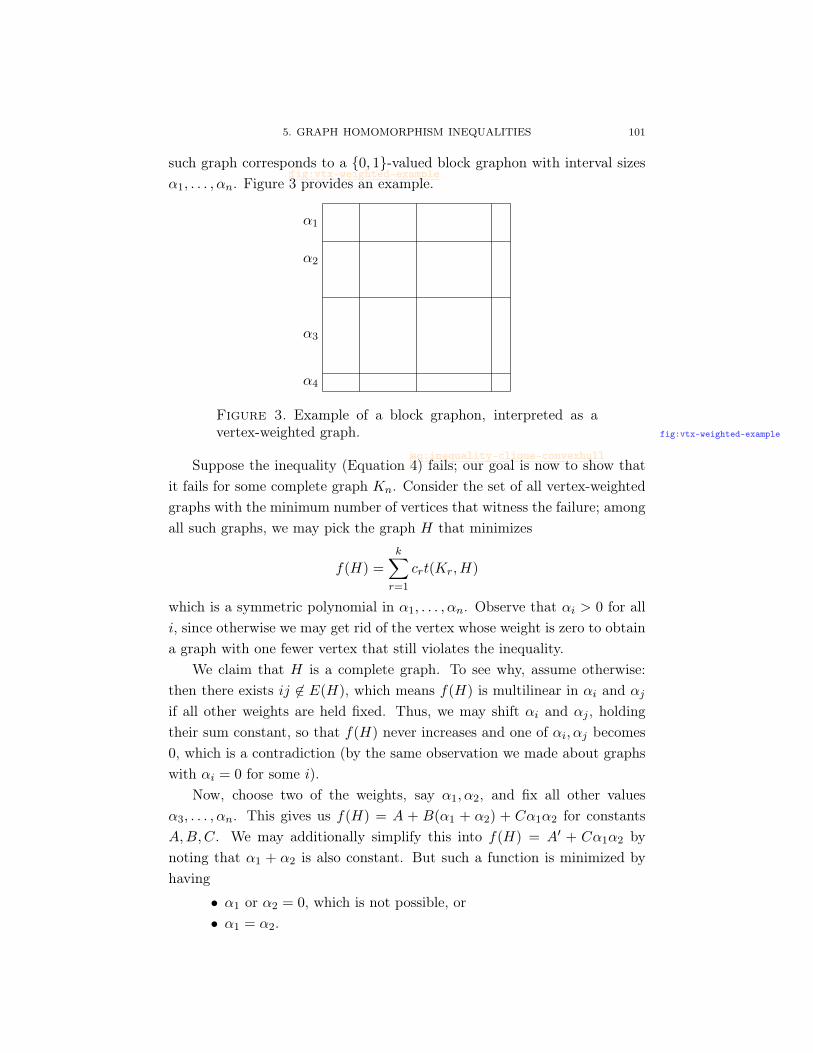
5. GRAPH HOMOMORPHISM INEQUALITIES 101
such graph corresponds to a 0, 1-valued block graphon with interval sizesα1, . . . , αn. Figure
fig:vtx-weighted-examplefig:vtx-weighted-example3 provides an example.
α1
α2
α3
α4
Figure 3. Example of a block graphon, interpreted as avertex-weighted graph. fig:vtx-weighted-example
Suppose the inequality (Equationeq:inequality-clique-convexhulleq:inequality-clique-convexhull4) fails; our goal is now to show that
it fails for some complete graph Kn. Consider the set of all vertex-weightedgraphs with the minimum number of vertices that witness the failure; amongall such graphs, we may pick the graph H that minimizes
f(H) =k∑r=1
crt(Kr, H)
which is a symmetric polynomial in α1, . . . , αn. Observe that αi > 0 for alli, since otherwise we may get rid of the vertex whose weight is zero to obtaina graph with one fewer vertex that still violates the inequality.
We claim that H is a complete graph. To see why, assume otherwise:then there exists ij 6∈ E(H), which means f(H) is multilinear in αi and αjif all other weights are held fixed. Thus, we may shift αi and αj , holdingtheir sum constant, so that f(H) never increases and one of αi, αj becomes0, which is a contradiction (by the same observation we made about graphswith αi = 0 for some i).
Now, choose two of the weights, say α1, α2, and fix all other valuesα3, . . . , αn. This gives us f(H) = A + B(α1 + α2) + Cα1α2 for constantsA,B,C. We may additionally simplify this into f(H) = A′ + Cα1α2 bynoting that α1 + α2 is also constant. But such a function is minimized byhaving
• α1 or α2 = 0, which is not possible, or• α1 = α2.
102 5. GRAPH LIMITS
This tells us that all αi’s are equal, which devolves into the symmetric com-plete graph Kn.
cor:convex-hull-Kn Corollary 5.56. For each m, the extreme points of the convex hull of
(t(K2,W ), . . . , t(Km,W )) : graphons W
are(t(K2,Kn), . . . , t(Km,Kn)) : n ≥ 1 ∪ (1, . . . , 1).
(Note: The extra point (1, . . . , 1) comes from the limit as n→∞.)Intuitively, the result tells us that in order to optimize any linear com-
bination of clique densities, subject to linear constraints on other cliquedensities, one simply has to check the inequalities at the cliques. With a bitof straightforward calculation, one can deduce Turán’s theorem, which canbe formulated as
t(Kr+1,W ) = 0 =⇒ t(K2,W ) ≤ 1− 1r .
It also allows us to begin to draw a more complete picture of set of possibleedge and triangle densities (Figure
fig:k2k3-density-plot-completefig:k2k3-density-plot-complete4). We may plug in m = 3 to infer that
the convex hull of the region has extreme points(1− 1
n,(n− 1)(n− 2)
n2
): n ≥ 1
∪ (1, 1).
All of these points lie on the parabola y = x(2x−1) (the fact that the regionlies above this parabola was a problem on your first problem set).
The curves that bound from below in the regime t(K2,W ) > 0.5 is asequence of cubic curves, due to Razborov’s theorem (Theorem
th:razborov-hom-densityth:razborov-hom-density5.57), which
we state without proof.
th:razborov-hom-density Theorem 5.57 (Razborov). For fixed t(K2,W ) ∈ [1 − 1k−1 , 1 − 1
k ], the minof t(K3,W ) is attained by a complete graph with node weights α1, . . . , αk,where α1 = α2 = · · · = αk−1 ≥ αk.
Remark 5.58. Unless t(K2,W ) = 1 − 1k , such a graph is not unique, since
we may replace a 0 − 1 triangle-free graphon with any other triangle-freegraphon, making sure it is distinct by scaling it by some β > 0.
Lec17: BrynmorChapman and Jerry Li
Razborov’s bound is very recent, and quite technical. This result hasbeen generalized to K2 vs K4 by Nikiforov. Reiher later extended it to K2
vs Kr for any r.
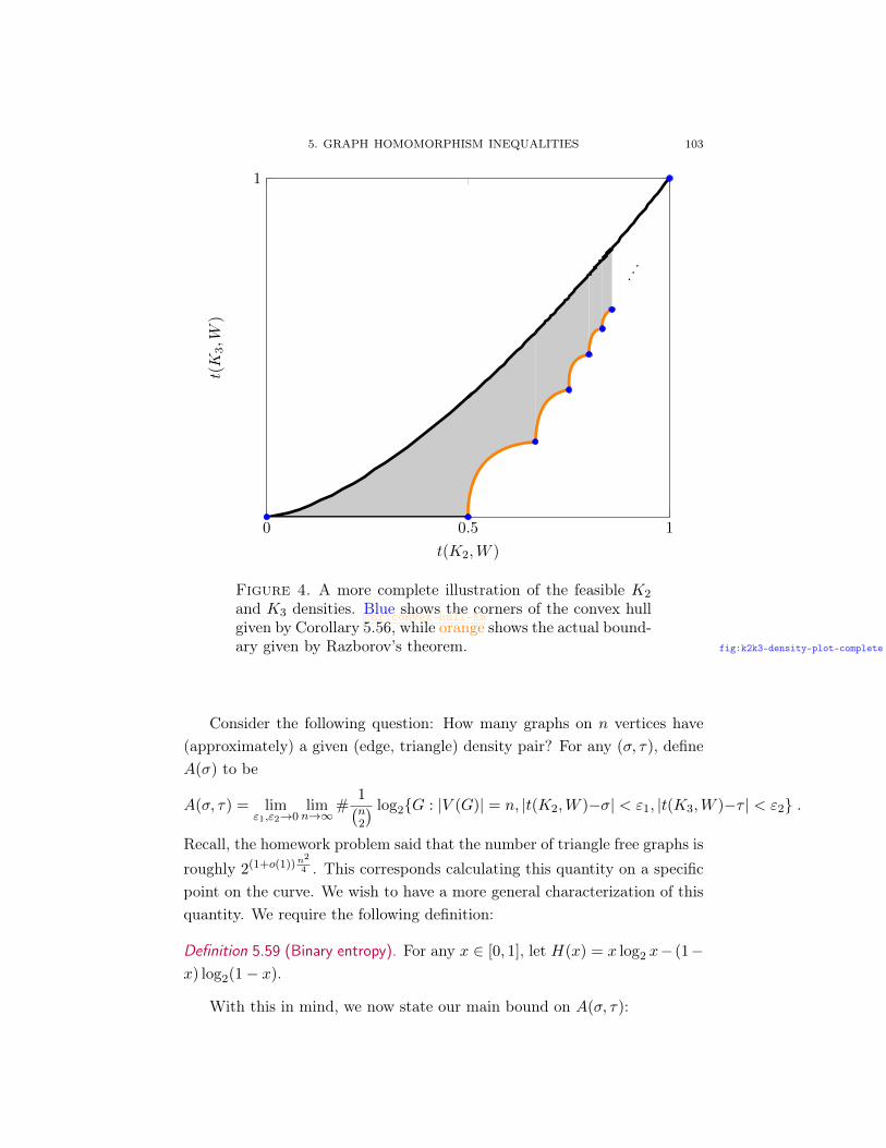
5. GRAPH HOMOMORPHISM INEQUALITIES 103
0 0.5 1
1
···
t(K2,W )
t(K
3,W
)
Figure 4. A more complete illustration of the feasible K2
and K3 densities. Blue shows the corners of the convex hullgiven by Corollary
cor:convex-hull-Kncor:convex-hull-Kn5.56, while orange shows the actual bound-
ary given by Razborov’s theorem. fig:k2k3-density-plot-complete
Consider the following question: How many graphs on n vertices have(approximately) a given (edge, triangle) density pair? For any (σ, τ), defineA(σ) to be
A(σ, τ) = limε1,ε2→0
limn→∞
#1(n2
) log2G : |V (G)| = n, |t(K2,W )−σ| < ε1, |t(K3,W )−τ | < ε2 .
Recall, the homework problem said that the number of triangle free graphs isroughly 2(1+o(1))n
2
4 . This corresponds calculating this quantity on a specificpoint on the curve. We wish to have a more general characterization of thisquantity. We require the following definition:
Definition 5.59 (Binary entropy). For any x ∈ [0, 1], let H(x) = x log2 x− (1−x) log2(1− x).
With this in mind, we now state our main bound on A(σ, τ):
104 5. GRAPH LIMITS
Theorem 5.60. For any σ, τ , we have:
A(σ, τ) = supW
∫H(W (x, y))dxdy : graphon W with t(K2,W ) = σ, t(K3,W ) = τ
.
(5) eq:graphon-density
We pause to make a couple of remarks about this statement. Observe thatfor a fixed x ∈ [0, 1], we have(
N
xN
)= 2N(H(x)+o(1)) , as N →∞ ,
where we interpret the LHS approximately by rounding xN if necessary.Hence the above statement qualitatively says that the exponent in A(σ, τ)
is highly controlled by a single graphon.By compactness, the supremum is always attained by some graphon.This is very general. In particular, the equality holds for any graphs, not
just K2,K3. This is also related to a conjecture of Sidorenko:
Conjecture 5.61 (Sidorenko’s conjecture). If H is bipartite, W graphon, thent(H,W ) ≥ t(K2,W )|E(H)| .
We remark we have already seen this for H = C4. In the problem setwe will show this for some others. However, in general, we do not knowwhether this holds for all H. One concrete example we do not know thisfor is H = K5,5 \ C10. This graph has a name: it is called the Möbiusstrip. This is because corresponds to the vertex-face incidence graph of theminimal simplicial complex of the Möbius strip.
One reason why these theorems are so hard is because they are in generalundecidable:
thm:hatami-norime Theorem 5.62 (Hatami-Norime). It is algorithmically undecidable whetheran inequality of the form
k∑i=1
cit(Hi, G) ≥ 0 (6) eq:lin-eq-graphons
holds for all graphs G.
Observe this holds in direct contrast to the case when the Hi’s are all cliques,as we saw last time. This is deduced from Matiyasevich’s theorem, which

5. GRAPH HOMOMORPHISM INEQUALITIES 105
proved the undecidablity of Hilbert’s 10th problem. The proof of Theo-rem
thm:hatami-norimethm:hatami-norime5.62 follows by cleverly encoding Diophantine equations in these in-
equalities at very specific points. The rough idea is to use the vertices ofthe region in Figure
fig:k2k3-density-plot-completefig:k2k3-density-plot-complete4 to encode integer solutions to diophantine equation-
s/inequalities.On the other hand we have:
Theorem 5.63. There is an algorithm so that, for every ε > 0, decides thateither
k∑i=1
cit(Hi, G) ≥ −ε , (7) eq:lin-eq-graphons-approx
or produces a G for which this inequality fails.
Proof. Apply the weak regularity lemma with some ε′ ε. This impliesthat we only need to check this for all graphons which are step graphonswith side length ε′. Then check the possibilities. If (
eq:lin-eq-graphonseq:lin-eq-graphons6) holds for all such
graphons, then by the counting lemma, then (eq:lin-eq-graphons-approxeq:lin-eq-graphons-approx7) holds for all graphs, by the
counting lemma. Otherwise we have produced a counterexample.


CHAPTER 6
Roth’s theorem
Let r3([N ]) denote the maximum size subset of [N ] that does not have a3-AP. Recall Roth’s theorem states that r3([N ]) = o(N). We proved this inclass using the triangle removal lemma, but this is not how Roth originallyproved it.
We now note the history of this theorem. The original proof showed:
Theorem 6.1 (Roth’53). r3([N ]) = O(N/ log logN).
In the 90’s, it was shown that:
Theorem 6.2 (Szemeredi’90, Heath-Brown’87). r3([N ]) = O(N/ logcN) forsome constant c > 0.
In work of Bourgain in ’99 and ’08 and later Sanders in ’12, c was im-proved to 1/2 + o(1) then 2/3 + o(1) and 3/4 + o(1). Finally, Sanders ’11showed:
Theorem 6.3 (Sanders’11). r3([N ]) = O(N(log logN)6/ logN).
Later Bloom ’16 improved this to O(N(log logN)4/ logN). It is a majoropen problem whether we can improve this beyond O(N/ logN). This isrelated to a famous conjecture of Erdős:
Conjecture 6.4 (Erdős). Suppose A ⊆ N satisfies∑
a∈A1a = ∞. Then A
contains arithmetic progressions of arbitrary size.
Observe that the hypothesis roughly corresponds toA having densityO(N/ logN).There is a finite field analog of Roth’s theorem. Define r3(Fn3 ) to be the
size of the largest subset S of Fn3 without a solution to x−2y+z = 0 for dis-tinct x, y, z ∈ S. (Note that this is equivalent to x+y+z = 0 in characteristic3.) Brown and Buhler showed in ’84 that r3(Fn3 ) ∈ o(3n). Meshulam ’95 thenshowed that r3(Fn3 ) ∈ O(3n/n). This was improved by Bateman-Katz ’12,
107

108 6. ROTH’S THEOREM
which showed that in fact r3(Fn3 ) ∈ O(3n/n1+c) for some c > 0. There wasthen a significant breakthrough of Croot-Lev-Pach ’17 which showed thatfor a slightly different problem, i.e. replacing Fn3 with (Z/4Z)n, there wasan exponential improvement r3((Z/4Z)n) ≤ 40.926n. A week later Ellenberg-Gijswijt showed that this implied that r3(Fn3 ) ≤ (2.756)n.
§6.1 Roth’s theorem in Fn3thm:meshulam Theorem 6.5 ( [30]). If A ⊂ Fn3 has no 3-APs, then |A| = O(3n/n).
The key advantage of this model is that this space has subspaces. Thekey idea is the following dichotomy: either the associated function is Fourieruniform, which by a counting lemma will imply there are many 3-APs, orthere is some large Fourier coefficient γ. Then, looking at V = γ⊥, thecodimension 1 subspace of this coefficient, our density should increment insome coset of V . Since codimension 1 subspaces of Fn3 are just Fn−1
3 , we caniterate this argument.
Let us recall some notation on Fourier transforms on finite abelian groups.Let f : Γ → C, and let γ ∈ Γ. Recall f(γ) = 〈f, γ〉 = Ex∈Γf(x)γ(x). Inparticular, when Γ = Fn3 , we have Γ ∼= Fn3 , and for any γ ∈ Fn3 , we have
f(γ) = Ex∈Fn3 f(x)ω−γ·x ,
where ω is a primitive 3rd root of unity. The key identity that allows us torelate Fourier analysis to arithmetic progressions is the following:
Theorem 6.6. Let f, g, h : Γ→ C. Let
Λ(f, g, h) = Ex,y∈Γf(x)g(x+ y)h(x+ 2y) .
ThenΛ(f, g, h) =
∑γ∈Γ
f(γ)g(γ−2)h(γ) .
6. ROTH’S THEOREM IN Fn3 109
Proof. We will use the Fourier inversion formula, which says that f(x) =∑γ∈Γ f(γ)γ(x). Expand the LHS using this formula:
Λ(f, g, h) = Ex,y∈Γf(x)g(x+ y)h(x+ 2y)
= Ex,y
(∑γ1
f(γ1)γ1(x)
)(∑γ2
g(γ2)γ2(x+ y)
)(∑γ3
h(γ3)γ3(x+ 2y)
)=
∑γ1,γ2,γ3∈Γ
f(γ1)g(γ2)h(γ3)Ex,yγ1(x)γ2(x)γ2(y)γ3(x)γ3(y)2
=∑
γ1,γ2,γ3∈Γ
f(γ1)g(γ2)h(γ3)(Ex(γ1γ2γ3)(x)
)(Ey(γ2γ
23)(y)
)Recall that the expectation of a character γ is 1 if γ ≡ 1 and 0 otherwise.Hence all terms in the final sum vanish except those for which γ1γ2γ3 ≡ 1
and γ2γ23 ≡ 1. This gives:∑
γ1,γ2,γ3∈Γ
f(γ1)g(γ2)h(γ3)(Ex(γ1γ2γ3)(x)
)(Ey(γ2γ
23)(y)
)=∑γ∈Γ
f(γ)g(γ−2)h(γ)
This completes the proof.
For Γ = Fn3 , observe that x− 2y + z = x+ y + z. So we are just tryingto count
1
32n|x+ y + z = 0, x, y, z ∈ A| = Ex,d1A(x)1A(x+ d)1A(x+ 2d) .
By applying the identity, we have
Ex,d1A(x)1A(x+ d)1A(x+ 2d) =∑γ∈Fn3
1A(γ)21A(−2γ) =∑γ
1A(γ)3 .
If A ⊂ Fn3 is 3-AP free, let |A| = αN where N = 3n. Recall that thefirst step is to show that if there are few 3-APs, then there is a large Fouriercoefficient. Recall we need to count trivial 3-APs, so if A is 3-AP free, thenthe number of 3-APs is exactly |A| = αN . Since α = 1A(0), by our identity

110 6. ROTH’S THEOREM
we have1
N2|x+ y + z = 0| =
∑γ
1A(γ)3 = α3 +∑γ 6=0
1A(γ)3
≥ α3 −maxγ 6=0|1A(γ)|
∑γ
1A(γ)2
= α3 −maxγ 6=0|1A(γ)| E
x1A(x)2
= α3 −maxγ 6=0|1A(γ)|α .
In other words, if A is 3-AP free, then there exists some γ 6= 0 so that
|1A(γ)| ≥ α2 − 1
N≥ α2
2
provided that N ≥ 2α2 .
Now recall the second step is that such a Fourier coefficient should implya density increment on a codimension 1 subspace. This is formalized in thefollowing lemma:
Lemma 6.7. Let A ⊆ Fn3 with |A| = αN . Let γ 6= 0 with |1A(γ)| ≥ δ. ThenA has density ≥ α+ δ
2 on a codimension-1 subspace.
Proof. By definition, we have
1A(γ) = Ex∈FN3 1A(x)ω−γ·x
=1
3
(α0 + α1ω + α2ω
2)
where α0, α1, α2 are the densities of A on the three cosets of V = r⊥. Recall13(α0 + α1 + α2) = α. Hence
3δ ≤ |α0 + α1ω + α2ω2|
= |(α0 − α) + (α1 − α)ω + (α2 + α)ω2|
≤2∑j=0
|αj − α|
=
2∑j=0
|αj − α|+ (αj − α) .
Since every term in the sum is nonnegative, this implies that there exists jso that |αj − α|+ (αj − α) ≥ δ which implies αj ≥ α+ δ/2.
Lec18: Jonathan Tidorand Nicole Wein

6. ROTH’S PROOF OF ROTH’S THEOREM 111
Proof of Theoremthm:meshulamthm:meshulam6.5. Combining the arguments above, we have shown that
if A ⊆ Fn3 with no 3-APs, writing N = 3n and |A| = αN , if N ≥ 2/α2
then Fn3 contains a coset of a codimension 1 subspace, V + v, such that|A ∩ (V + v)| ≥ (α+ α2/4)|V + v|.
Write A′ = A ∩ (V + v). Let A1 = A′ − v = a− v : a ∈ A′. Note thatA1 ⊆ V ∼= Fn−1
3 has no 3-APs since if a, b, c ∈ A′ with (a − v) + (b − v) +
(c− v) = 0, then a+ b+ c = 0 (since we are working over F3 where 3v = 0),contradicting the fact that A is 3-AP-free.
Therefore starting with A = A0 ⊆ Fn3 with density α = α0, we have pro-duced A1 ⊆ Fn−1
3 with density α1 ≥ α0 +α20/4. Furthermore, A1 remains 3-
AP-free so we can iterate this argument, producing a sequence A0, A1, A2, . . .
with Ai ⊆ Fn−i3 with densities αi satisfying αi+1 ≥ αi + α2i /4. This process
continues as long as 3n−i ≥ 2/α2i . In addition, αi ≤ 1 since this quantity is
a density, so this process cannot continue forever. Careful analysis will givea precise bound on |A| = αN .
Since αi+1 ≥ αi(1 + αi/4) then αi doubles in at most d4/αie steps, i.e.,αi+d4/αie ≥ 2αi. Then since the αi’s are increasing, they start doublingfaster. Let ij = d4/αe + d2/αe + · · · + d23−j/αe. Then αij ≥ 2jα. Inparticular, this process must halt after at most ilog2(1/α) steps. Write k =
ilog2(1/α) ≤ 8/α+ log2(1/α).When the process halts, this means that 3n−k < 2/α2
k < 2/α2. Combin-ing these facts, we know that
n < log3(2/α2) + k ≤ 8/α+ log2(1/α) + log3(2/α2) = O(1/α).
This implies that α = O(1/n), so |A| = αN = O(3n/n), as desired.
Remark 6.8. If we were being sloppy, we could use the bound αi ≥ iα2/4,which implies that the process must stop after 4/α2 steps. This leads tothe worse bound |A| = O(3n/
√n), so careful analysis of this process is
necessary to get the correct bounds. If we were even more careful with theargument and the analysis of it, we could recover Meshulam’s original boundof r3(Fn3 ) ≤ 2 · 3n/n.
§6.2 Roth’s proof of Roth’s theorem
Theorem 6.9 ( [40]). r3([N ]) = O(N/ log logN).
The proof will have the same three steps as in Fn3 , but all the steps willbe slightly trickier:
112 6. ROTH’S THEOREM
(1) few 3-APs implies large Fourier coefficient assuming N is large;(2) large Fourier coefficient implies density increment on a fairly large
arithmetic sub-progression;(3) iterate the argument on the sub-progression.
The proof uses Fourier analysis on Z. The group of characters Z ∼= R/Z isnot discrete so there will be some integrals but everything works out basicallythe same as for finite abelian groups.
For t ∈ R/Z, define e(t) : Z → C by e(t) = e2πit. For simplicity we onlyconsider functions f : Z→ C that are non-zero at finitely-many points. Thenf : R/Z→ C is defined by
f(θ) =∑n∈Z
f(n)e(−nθ).
(Note that by assumption this sum only contains finitely-many non-zeroterms. This means we can ignore some annoying details involving integralsof infinite sums.)
We will use the following fact which relates the Fourier coefficients of fto the number of weighted 3-APs that f has. Define
T (f, g, h) =∑x,y∈Z
f(x)g(x+ y)h(x+ 2y).
ThenT (f, g, h) =
∫R/Z
f(θ)g(−2θ)h(θ) dθ.
We write T (f) for T (f, f, f).
Remark 6.10. It is possible to do this proof without using Fourier analysis onZ by instead embedding [N ] into Z/(2N + 1)Z. It does not make very muchdifference at the end, though doing Fourier analysis in Z feels more naturalfor this problem.
§6.2.1 Large Fourier coefficient. The following proposition should feel sim-ilar to the counting lemma. It says that if two functions are similar then theyhave a similar number of 3-APs.
thm:integer-counting Lemma 6.11. If f, g : Z→ C satisfy∑
n∈Z |f(n)|2,∑n∈Z |g(n)|2 ≤M , then
|T (f)− T (g)| ≤ 3M‖f − g‖∞.
6. ROTH’S PROOF OF ROTH’S THEOREM 113
Proof. T (f)− T (g) telescopes as
T (f, f, f)− T (g, g, g) = T (f − g, f, f) + T (g, f − g, f) + T (g, g, f − g).
Each term is bounded by M‖f − g‖∞ in absolute value. We prove this forthe first term.
|T (f − g, f, f)| =∣∣∣∣∫ 1
0f − g(θ)f(−2θ)f(θ)
∣∣∣∣ dθ≤ ‖f − g‖∞|
∫ 1
0|f(−2θ)f(θ)| dθ
≤ ‖f − g‖∞(∫ 1
0|f(−2θ)|2 dθ
)1/2(∫ 1
0|f(θ)|2 dθ
)1/2
(Cauchy-Schwarz)
= ‖f − g‖∞∫ 1
0|f(θ)|2 dθ
= ‖f − g‖∞∑n∈Z|f(n)|2 (Parseval)
≤M‖f − g‖∞.
Now if A ⊆ [N ] has no 3-APs with |A| = αN , then T (1A) only countstrivial 3-APs, so T (1A) = αN . However T (α1[N ]) ≥ α3N2/2, i.e., is large.By Lemma
thm:integer-countingthm:integer-counting6.11, this implies that 1A − α1[N ] must have a large Fourier
coefficient.In particular, we apply Lemma
thm:integer-countingthm:integer-counting6.11 with M = αN , implying that
‖ 1A − α1[n]‖∞ ≥(α3N2/2− αN)
3αN= α2N/6− 1/3.
This is at least α2N/10 if N ≥ 5/α2.Therefore we have shown that if N ≥ 5/α2, then there exists θ ∈ R such
that ∣∣∣∣∣N∑n=1
(1A − α)(n)e(θn)
∣∣∣∣∣ ≥ α2
10N.
§6.2.2 Density increment. The following lemma says that a large Fouriercoefficient implies a density increment on a large arithmetic sub-progression.
lem:2 Lemma 6.12. If |1A(r)| ≥ δ for some r 6= 0, then A has density at leastα+ δ
2 on a codimension 1 coset.
114 6. ROTH’S THEOREM
The idea of the proof of Lemmalem:2lem:26.12 is as follows. Previously we saw
that in the finite field setting, a large Fourier coefficient divides up the spaceinto three cosets where the character is constant on each coset. Here, wedon’t have the property that the character is constant, but we will be ableto find arithmetic sub-progressions such that the character is approximatelyconstant. We will partition [N ] into arithmetic progressions of length aboutN1/3 such that e(nθ) is approximately constant on each progression. To getintuition for why this is possible, consider how f(θ) behaves. It jumps aroundthe unit circle and when θ is close to a fraction with small denominator, it isalmost periodic which means that e(nθ) is approximately constant. Thus, wefirst approximate θ by a fraction with small denominator using the followinglemma.
lem:dir Lemma 6.13 (Dirichlet). Let θ ∈ R and 0 < δ < 1. Then there exists apositive integer d ≤ 1
δ such that ||dθ||R/Z ≤ δ where ||x||R/Z denotes distancefrom x to the nearest integer.
Proof. Let m = b1δ c and consider 0, θ, 2θ, . . . , mθ. By the pigeonhole
principle, some pair iθ, jθ differ by at most δ in their fractional parts. Taked = |i− j|. Then ||dθ||R/Z ≤ δ.
Now we show how to partition [N ] into sub-progressions so that thecharacter is approximately constant on each sub-progression.
lem:pro Lemma 6.14. Let 0 ≤ η ≤ 1 and θ ∈ R. Suppose N > Cη6 . Then it is
possible to partition [N ] into sub-progressions Pi of length at least N1/3 suchthat supx,x′∈Pi |e(θx)− e(θx′)| ≤ η for all i.
Proof. The idea is that if you have an arithmetic progression whose commondifference induces a character very close to 1 then the character won’t changemuch on this progression. If P is an arithmetic progression with commondifferent d then by the triangle inequality
supx,x′∈P
|e(θx)− e(θx′)| ≤ |P | · |e(θd)− 1|
≤ |P | · 2π · ||dθ||R/ZTo see the last inequality, notice that |e(t)−1| is a chord length and 2π||t||R/Zis the corresponding arc length.
6. ROTH’S PROOF OF ROTH’S THEOREM 115
We’ll form pretty short arithmetic sub-progressions whose common dif-ferences are close to a fraction, that is, dθ is close to an integer. Thatis, if N1/3 ≤ |P | ≤ 2N1/3 and ||dθ||R/Z ≤ η
2π|Pi| , then we’re done. Ap-
plying Lemmalem:dirlem:dir6.13 with N ≥ C
η6 , we can find d ≤ 4πN1/3
η ≤√N such
that ||dθ||R/Z < η4πN1/3 ≤ η
2π|P | . Given such a d, we partition [N ] into sub-progressions of common difference d of lengths between N1/3 and 2N1/3.
Now we’ll use the above lemmas to get a density increment, provingLemma
lem:2lem:26.12.
Proof of Lemmalem:2lem:26.12. Recall that there exists θ ∈ R such that |∑x∈[N ](1A−
α)(x)e(θx)| ≥ α2
10N with a partition of [N ] into arithmetic sub-progressionsPi as in Lemma
lem:prolem:pro6.14. We will argue that one of these sub-progressions
witnesses a density increment. The key point will be that for each of thesesub-progressions the character deviates by at most η. We have,
α2
10N ≤
∣∣∣∣∣∣∑x∈[N ]
(1A − α)(x)e(θx)
∣∣∣∣∣∣≤
k∑i=1
∣∣∣∣∣∣∑x∈Pi
(1A − α)(x)e(θx)
∣∣∣∣∣∣≤
k∑i=1
∣∣∣∣∣∣∑x∈Pi
(1A − α)(x)
∣∣∣∣∣∣+α2
20|Pi|
Note that the error term
∑ki=1
α2
20 |Pi| = α2
20N is only half of our originalbound α2
10N . The idea is that we have a lower bound on the average densitydeviation from α over all Pi and will use this to conclude that one of thesub-progressions must have much bigger density than α. In the finite fieldsetting, we simply used the pigeonhole principle to show existence of such asub-progression, but here naively applying the pigeonhole principle will notbe strong enough. We bound the error term as follows.
k∑i=1
α2
20|Pi| ≤
k∑i=1
∣∣∣∣∣∣∑x∈Pi
(1A − α)(x)
∣∣∣∣∣∣=
k∑i=1
(∣∣|A ∩ Pi| − α|Pi|∣∣+ (|A ∩ Pi| − α|Pi|))
116 6. ROTH’S THEOREM
In the last equality, we use the trick of adding the quantity to itself withoutthe absolute value. We can do this because it averages to 0 and it is helpfulbecause now each term is non-negative.
Now by the pigeonhole principle, there exists i such that ||A ∩ Pi| − α|Pi||+(|A ∩ Pi| − α|Pi|) ≥ α2
20 |Pi|. So |A ∩ Pi| ≥ (α + α2
40 )|Pi|. Thus, if A ⊂ [N ] is3-AP-free and N > Cα−12 then |A ∩ P | ≥ (α+ α2
40 )|P |. for some arithmeticsub-progression P of size at least N1/3.
§6.2.3 Iteration. We now iterate the density increment. The recurrence isas follows. N0 = N , α0 = α, P = [N ], Ni+1 ≥ N
1/31 , αi+1 ≥ αi(1 + αi
40),|Pi| = Ni. The density doubles after at most 40
α steps and doubles againafter at most 20
α steps etc., resulting in a total of at most 80α steps. When
the process stops it must stop because the condition on N is violated, thatis, Ni ≤ Cα−12
i ≤ Cα−12. Thus, N ≤ (Cα−12)380/α= ee
O(1/α) so α =
O( 1log logN ). This completes the proof of Roth’s Theorem.
§6.2.4 Comparison between Roth’s Theorem for Fn3 and [N ]. In the caseof Fn3 , we got a bound on the order of N
logN where N = 3n while in the caseof [N ] we got a bound on the order of N
log logN . This extra log factor comesfrom the fact that for Fn3 we restricted to a subspace of 1/3 fraction in size,where as for [N ] we restricted to a much smaller progression of size N1/3.This raises the question of whether sub-progressions are the “correct” analogof subspaces for [N ]. It turns out they are not and instead the correct analogis something called a Bohr set. Bourgain introduced Bohr sets for improvingbounds on Roth’s theorem in [N ].
We define Bohr sets as an analog to subspaces. One way to specify asubspace is as follows. Given characters r1, r2, . . . , rk ∈ Fn3 , a subspace isthe set x ∈ Fn3 |x · rj = 0 ∀j. Similarly, we can specify a Bohr set asfollows. Given characters γ1, γ2, . . . , γk ∈ Γ, a Bohr set is the set x ∈Γ∣∣| arg γj(x)| < 2πρ ∀j. Unfortunately, Bohr sets are more difficult to work
with than subspaces. One reason for this is that subspaces are preservedunder addition, but the same is not true for Bohr sets. You should think ofa Bohr set kind of like a ball of radius ρ. Addition two elements of such a balltogether gives a point in the ball of radius 2ρ, not the original ball. Despitethese difficulties Bohr sets can be used to greatly improve the bounds onr3([N ]).Lec19: Kevin Sun and
Meghal Gupta

6. OTHER APPROACHES TO ROTH’S THEOREM OVER Fn3 117
§6.3 Other approaches to Roth’s theorem over Fn3We now return to the problem of giving bounds on the sizes of subsets
A ⊂ Fn3 with no three-term arithmetic progression. The following betterupper bound was found in 2012.
thm:bateman-katz Theorem 6.15 (Bateman-Katz). For A ⊂ Fn3 with no 3-AP’s, we have |A| =O(
3n
n1+c) for some c > 0.
There has also been some progress on the converse problem, finding alarge subset of Fn3 with no 3-AP’s.
thm:edel Theorem 6.16 (Edel). There exists A ⊂ Fn3 with no 3-AP’s such that |A| ≥2.217n for all sufficiently large n.
This lower bound was proven by taking a specific finite construction andtensoring it up to constructions for larger n.
However, more recently, a completely different method has improvedthe upper bound significantly. We show this proof found by Ellenberg andGijswijt below.
thm:capset Theorem 6.17. For A ⊂ Fn3 with no 3-AP’s, we have |A| = O(2.756n).
To prove this result, we use a general technique which is sometimesreferred to as the polynomial method.
Suppose A ⊂ Fn3 is 3-AP free (i.e. no x + y + z = 0). We can encodethis fact in a different way by noting that when A is 3-AP free, then for allx, y, z ∈ A,
δ0(x+ y + z) =∑a∈A
δa(x)δa(y)δa(z)
where δa = 1 if x = a and 0 otherwise.Now, we define the notion of “slice rank” for a function, and we will show
that the left hand side of the above expression has “low slice rank” while theright side has “high slice rank”.
Definition 6.18. Consider functions F : A × A × A . . . × A → F (with k
A’s) for some field F. We say that a function F has slice-rank 1 if F hasthe form F (x1, x2, . . . xk) = f(xj)g(x1, x2, . . . xj−1, xj+1, . . . xk−1, xk) (e.g.f(x1)g(x2, x3, . . . xk) or f(x2)g(x1, x3, x4, . . . xk) or f(x3)g(x1, x2, x4, x5, . . . xk)

118 6. ROTH’S THEOREM
etc.). The slice rank of a general function F : A×A×A . . .×A→ F is theminimum r such that F can be written as the sum of r slice-rank 1 functions.
Remark 6.19. Note that this is analogous to the usual notion of rank of amatrix, which can be defined as follows. We say that F : A × A → Fhas rank 1 if F (x, y) = f(x)g(y) for some f, g : A → F. Then definerankF = minr : F = F1 + · · ·+ Fr, Fihas rank1.
Lemma 6.20 (Slice-rank of a diagonal tensor is high). Consider coefficientsca ∈ F, indexed by elements in A ⊆ F. Let F (x1, x2, . . . xk) =
∑a∈A caδa(x1) · · · δa(xk).
Then the slice-rank of F is exactly the number of ca that are nonzero.
Proof. One direction is clear, as the slice rank of F must be at most |a ∈A : ca 6= 0|.
We prove the other direction using induction on k.For k = 2, this reduces to standard linear algebra. Now suppose we have
k > 2 and we have already proven the claim for smaller k. First delete fromA all a ∈ A for which ca = 0. The slice-rank does not increase.
Suppose, for contradiction, that the slice rank is at most |A| − 1, so thatwe can write
∑a∈A caδa(x1) · · · δa(xk) as a sum of rank 1 functions.
Then we can group these by xi and write∑a∈A
caδa(x1) · · · δa(xk) =
k∑i=1
∑α∈Ii
fi,α(xi)gi,α(x1, x2, . . . , xi−1, xi+1, . . . , xk)
where |I1|+ · · ·+ |Ik| ≤ |A| − 1.In order to apply induction, we want to remove the contributions of one
such Ik. Consider the orthogonal space to fk,α which is defined by
I⊥k = h : A→ F :∑x∈A
fk,α(x)h(x) = 0 for all α ∈ Ik.
The dimension of I⊥k as a vector space must be at least |A| − |Ik|. Considersome look at a basis of I⊥k . This gives rise to a matrix with dimensions(dim I⊥k )×A, which must contain some full rank minor. In particular, thereexists some h ∈ I⊥k with | supph| ≥ |A| − |Ik|.
Now multiply our expression from above by h(xk), and sum over xk ∈ A.After summing, we are left with∑a∈A
caδa(x1), · · · δa(xk−1)h(a) =
k−1∑i=1
∑α∈Ii
fi,α(xi)gi,α(x1, x2, . . . , xi−1, xi+1, . . . xk−1),

6. OTHER APPROACHES TO ROTH’S THEOREM OVER Fn3 119
where g =∑xk∈A
gi,α(x1, x2, . . . , xi−1, xi+1, . . . xk−1, xk)h(xk). Each of the
fi,αgi,α is a function with slice rank 1.By our induction hypothesis, the slice rank of the left-hand side is the
number of nonzero coefficients, which is the number of a with nonzero cah(a),or |supp h| ≥ |A| − |Ik|. However, the slice rank of the right-hand side≤ |I1|+ |I2|+ · · ·+ |Ik−1| ≤ |A| − |Ik| − 1, which finishes our proof.
Lemma 6.21. Let F (x, y, z) = δ0(x+ y+ z) be the function from A×A×Ato F3. Then the slice rank of F is at most
3
∑
a,b,c≥0a+b+c=nb+2c≤2n/3
n!
a!b!c!
Proof. Notice that δ0(x) = 1−x2 for x ∈ F3. Then we can write δ0(x+y+z)
as
δ0(x+ y + z) =n∏i=1
(1− (xi + yi + zi)2).
The right hand side is a polynomial of total degree 2n which is a linearcombination of monomials
xi11 xi22 · · ·xinn yji1 · · · yjnn zk1
1 · · · zknnBy the pigeonhole principle, at least one of the sums i1 +· · ·+in, j1 +· · ·+jn,or k1 + · · ·+ kn has sum at most 2n/3.
Now we consider the contributions from all terms with i1 + · · ·+ in ≤ 2n3 .
We can group these terms by i1, . . . , in and write the sum of those terms inthe form
∑α fα(x)gα(y, z), where α ranges over all (i1, . . . in) ∈ 0, 1, 2n
with i1 + · · ·+ in ≤ 2n3 . Each of these is a function with slice-rank 1.
The number of such α is exactly∑
a,b,c≥0a+b+c=nb+2c≤2n/3
n!
a!b!c!. In this formula, a, b, c
represent the number of 0, 1, 2 among the il. Repeating this for j1, . . . jn andk1, . . . , kn gives the desired bound.
Proof of Theoremthm:capsetthm:capset6.17. Now return to our original equation expressing the
fact that A contains no arithmetic progressions of length 3. For all x, y, z ∈
120 6. ROTH’S THEOREM
A,δ0(x+ y + z) =
∑a∈A
δa(x)δa(y)δa(z).
If we compare slice ranks on both sides, we have |A| ≤ 3
∑
a,b,c≥0a+b+c=nb+2c≤2n/3
n!
a!b!c!
.
Now fix some 0 ≤ x ≤ 1, and compare the sum to(1 + x+ x2)n
x2n/3. If we ex-
pand this using the multinomial theorem, each (a, b, c) with a + b + c = n
gives us a term(
n
a, b, c
)x0·ax1·bx2·cx−2n/3. Each term in our above sum is
bounded above by one of the terms in the multinomial expansion, as x ≤ 1
and b + 2c − 2n/3 ≤ 0. Therefore we are able to bound |A| above by
3 · (1 + x+ x2)n
x2n/3, for any choice of x < 1. The optimal value of x to choose
is around 0.593, which gives us a bound of |A| ≤ 3 · 2.756n.
Remark 6.22 (Asymptotics in final step). We can also use Stirling’s approxi-mation or Cramer’s theorem to finish here.
If a = (α + o(1))n, b = (β + o(1))n, c = (γ + o(1))n, thenn!
a!b!c!=(
α−αβ−βγ−γ + o(1))n.
One may recognize this as eH(α,β,γ), where H(α, β, γ) = −α logα −β log β − γ log γ is an entropy function.
Remark 6.23 (Generalizations). It is unknown if the polynomial method herecan be extended to any of the following settings:
• Z/NZ• 4-APs in Fn5 .• Corners ((x, y), (x+ d, y), (x, y + d))in FN2 × FN2 .

CHAPTER 7
Structure of set addition
§7.1 Definitions in additive combinatorics
In this chapter, we will be working in some ambient abelian group (usu-ally Fn2 , Z/nZ, or Z).
Definition 7.1. A + B = a + b : a ∈ A, b ∈ B and A − B = a − b : a ∈A, b ∈ B. Similarly for an integer k, we have kA = A+A+ · · ·+A wherethere are k terms in the sum, and k ·A = k · a : a ∈ A.
We will primarily be concerned about the sizes of these sets. The mostbasic question to ask is the following: if we have a set A ∈ Z with |A| = n,how large or small can A+A be?
We have the following easy inequality: for a finite set A ⊂ Z,
2n− 1 ≤ |A+A| ≤(n+ 1
2
).
The left hand side bound follows by considering the terms a1 + a1, a1 +
a2, · · · a1 + an and a2 + an, . . . , an + an, which are all distinct elements ofA+ A. Equality on the left hand side is achieved exactly when A forms anarithmetic progression.
The bound on the right hand side follows by simply considering all(n+1
2
)pairs of elements of A. Equality on the right hand side holds if A is a “Sidonset”, when there are no nontrivial solutions to a+ b = c+ d.
More interestingly, we can try to analyze sets A such that |A + A| ≤K|A| and determine properties of them. (We usually take K to be a fixedconstant.)
We now try to give some examples of sets that satisfy |A + A| ≤ K|A|for specific constants K.
By our bound above, an arithmetic progression A satisfies |A + A| =
2|A| − 1 ≤ 2|A|. Therefore arithmetic progressions fall into this category.More generally, we can try to construct sets A with small A + A based onthe idea of arithmetic progressions. The most straightforward way to extend
121
122 7. STRUCTURE OF SET ADDITION
this is to take the Cartesian product of arithmetic progressions. Doing thiswith k arithmetic progressions will give us a set in Zk and |A+A| ≤ 2k|A|.Using this, we can “project” this set A onto Z using some integer lineartransformation, which will give a subset of Z with the same property.
Definition 7.2. A generalized arithmetic progression (GAP) is a set of theform a0 + a1d1 + · · ·+ akdk : 0 ≤ ai ≤ Ni − 1, 1 ≤ i ≤ k. Note that someof these sums can coincide. We say that the GAP is proper if all
∏Ni sums
are distinct. We call k the dimension of the GAP and N1 · · ·Nk the size ofthe GAP (note that the size of the set may be smaller if the GAP is notproper)
It is an easy exercise that if A is a GAP of dimension k, then we have|A+A| ≤ 2k|A|.
gap-subset Example 7.3. Subsets of GAP’s: Consider A which is a subset of A′ whereA′ is a GAP of dimension k. Let k′ be such that A contains 1
K′ fraction ofA’s elements, or K ′|A| = |A′|. Then |A+A| ≤ |A′+A′| ≤ K|A′| = KK ′|A|.
It is natural to ask if we can give some classification of sets that satisfythe property |A+A| ≤ K|A| for some constant A. In fact, this is possible. Itturns out that all such A are contained in some generalized arithmetic pro-gression discussed above, and this result, in some rough sense a classificationresult for all sets with this property, is known as Freiman’s theorem.
Theorem 7.4 (Freiman’s theorem). For every K > 0 there exist d(K), f(K) >
0 such that if a finite set A ⊂ Z satisfies |A+A| ≤ K|A|, then A is containedin a generalized arithmetic progression of dimension at most d(K) and sizeat most f(K)|A|.
Remark 7.5. We call such problems “inverse problems”: we have some exam-ples of sets that satisfy some condition, but our question is whether everyset that satisfies this condition belongs to one of our examples.
Lec20: PakawutJiradilok
§7.2 Plünnecke–Ruzsa inequality
Freiman’s theorem describes the structure of a set with small doubling.One of our goals is to prove the theorem. To do so, we need a few tools.

7. PLÜNNECKE–RUZSA INEQUALITY 123
thm:Ruzsatri Theorem 7.6 (Ruzsa’s triangle inequality). If A, B, C are finite subsets of anabelian group Γ, then
|A| · |B − C| ≤ |A−B| · |A− C|.
Proof. We will construct an injection from the Cartesian product A×(B−C)
to (A − B) × (A − C). If d is an element of B − C, we pick arbitrarilyelements b(d) ∈ B and c(d) ∈ C such that d = b(d) − c(d). Define a mapφ : A× (B−C)→ (A−B)× (A−C) by (a, d) 7→ (a− b(d), a− c(d)). To seethat φ is injective, we note that if φ(a, d) = (x, y) is given, then d = y − xand a = x+ b(d). Thus, we can uniquely recover (a, d).
Remark 7.7. Note that we cannot use this trick to prove the similar inequality|A| · |B + C| ≤ |A + B| · |A + C|, although we will see soon that this istrue. The reason this trick would not work is because if we construct a mapφ′ : A × (B + C) → (A + B) × (A + C) by φ′(a, d) 7→ (a + b(d), a + c(d)),where b(d) ∈ B and c(d) ∈ C are chosen so that d = b(d)+c(d), then we willnot, in general, be able to uniquely recover (a, d) from (a+ b(d), a+ c(d)).
Remark 7.8. On the other hand, by simply switching A to −A, B to −B,or C to −C, we can easily show that |A| · |B − C| ≤ |A + B| · |A + C|,|A| · |B + C| ≤ |A+B| · |A− C|, and |A| · |B + C| ≤ |A−B| · |A+ C|.
Remark 7.9. Why is this called Ruzsa’s triangle inequality? If we writeρ(A,B) := log |A−B|√
|A|·|B|, then the inequality says ρ(B,C) ≤ ρ(A,B)+ρ(A,C),
which looks like the triangle inequality. However, do not take this observationtoo seriously, since ρ is not a distance. For example, ρ(A,A) 6= 0 for a generalset A.
In the following example, we will see how Ruzsa’s triangle inequality isuseful.
Example 7.10. Suppose we set B = C = 2A−A. We have |A| · |3A− 3A| ≤|2A− 2A|2. In particular, if |2A− 2A| ≤ K · |A|, then |3A− 3A| ≤ K2 · |A|.Similarly, if we set B = C = 3A− 2A, then we get
|5A− 5A||A| ≤
( |3A− 3A||A|
)2
.

124 7. STRUCTURE OF SET ADDITION
This shows that if we start with a set A for which the size |2A − 2A| isbounded by a constant factor of |A|, then we can conclude that a set of theform kA− kA also has its size bounded by a constant factor of |A|.
In general, we have an upper bound for the size of a set of the formkA− `A, when k and ` are non-negative integers, provided that A has smalldoubling, in the following inequality.
thm:PRineq Theorem 7.11 (Plünnecke-Ruzsa inequality). Let A be a finite subset of anabelian group, and let K be a positive real number. If |A+A| ≤ K · |A|, thenfor integers k, ` ≥ 0, |kA− `A| ≤ Kk+`|A|.
More generally, it is true that if |A + B| ≤ K · |A|, where A and B arefinite subsets of an abelian group, then |kB− `B| ≤ Kk+`|A|. We will provethis general version. The following proof, due to Petridis, uses the followingkey lemma.
Lemma 7.12. If X ⊆ A is a nonempty subset that minimizes |X+B||X| , and let
K ′ = |X+B||X| . Then, |X +B + C| ≤ K ′ · |X + C|, for all finite sets C.
We can think of this lemma via the idea of expansion ratio. Let Γ denotethe ambient abelian group we are working on. For each finite set Z ⊆ Γ,the operation “addition by B” sends Z to Z + B ⊆ Γ. We can consider theexpansion ratio |Z+B|
|Z| , for each Z. If we fix a finite set A ⊆ Γ, we can considera subset X ⊆ A which minimizes this expansion ratio under addition by B.The lemma says that, for any finite set C ⊆ Γ, the set X + C expands evenless than X does under addition by B.
Let’s see how the lemma implies the general version of the inequality.
Proof. (assuming the lemma) Take a nonempty subsetX ⊆ A that minimizesthe ratio |X+B|
|X| . Let K ′ = |X+B||X| . Note that by the choice of X, we have
K ′ ≤ K. Therefore, |X + B| ≤ K · |X|. The lemma says that X + B
expands less than X does under addition by B. Therefore, |X + 2B| ≤K · |X + B| ≤ K2 · |X|. By iteration, for every non-negative integer ` ≥ 0,we have |X + `B| ≤ K`|X|.
Now Ruzsa’s triangle inequality gives |X| · |kB − `B| ≤ |X + kB| · |X +
`B| ≤ Kk+`|X|2. Thus, |kB − `B| ≤ Kk+`|X| ≤ Kk+`|A|.
Next, we prove the key lemma.

7. PLÜNNECKE–RUZSA INEQUALITY 125
Proof. (of the key lemma) We proceed by induction on |C|.Base case. If |C| = 1, write C = c. Then, for any finite set W , the
set W + C = W + c is simply a translation by c, and thus |W + C| = |W |.Therefore, |X +B + C| = |X +B| ≤ K ′|X| = K ′|X + C|.
Induction step. Assume |C| > 1. Write C = C ′ ] c. Note that
X +B + C = (X +B + C ′) ∪ [(X +B + c) \ (Z +B + c)] ,
where Z = x ∈ X : x+B+ c ⊆ X+B+C ′. By minimality of X, we have|Z +B| ≥ K ′|Z|. Therefore,
|X +B + C| ≤ |X +B + C ′|+ |(X +B) \ (Z +B)|= |X +B + C ′|+ |X +B| − |Z +B|≤ K ′|X + C ′|+K ′|X| −K ′|Z|. (induction hypothesis)
Observe that X +C = (X +C ′)] [(X + c) \ (W + c)], where W = x ∈ X :
x + c ∈ X + C ′. Note here that unlike the equation for X + B + C abovethe union here is a disjoint union. We have the equality
|X + C| = |X + C ′|+ |X| − |W |.
By definition, W ⊆ Z. This gives
|X + C| ≥ |X + C ′|+ |X| − |Z|.
Using this inequality in the inequality above, we obtain |X + B + C| ≤K ′|X + C|, as desired.
With the key lemma, now we can prove “another triangle inequality” wementioned earlier.
Corollary 7.13. If A, B, C be finite subsets of an abelian group Γ, then
|A| · |B + C| ≤ |A+B| · |A+ C|.
Proof. The inequality is obvious when A is empty. Assume A 6= ∅. Considera nonempty subset X ⊆ A that minimizes |X+B|
|X| . Let |A+B||A| = K and
|X+B||X| = K ′ ≤ K. The key lemma gives
|B + C| ≤ |X +B + C| ≤ K ′ · |X + C|
≤ K ′ · |A+ C| ≤ K · |A+ C| = |A+B| · |A+ C||A| .

126 7. STRUCTURE OF SET ADDITION
§7.3 Freiman’s theorem in abelian groups with boundedexponent
The next is an important tool.
thm:Ruzsacover Theorem 7.14 (Ruzsa’s covering lemma). Let A and S be finite subsets ofan abelian group such that S 6= ∅. Let K be a positive real number. If|A + S| ≤ K · |S|, then there exists a subset T ⊆ A with |T | ≤ K andA ⊆ T + S − S.
Roughly speaking, this theorem says that if the expansion ratio of S byaddition of A is at most K, then we can cover A by K translates of S − S.
Proof. The idea of this proof is to find a maximal packing. It appears thata maximal packing leads to a good covering, in the sense that we are goingto observe here.
Let T ⊆ A be a maximal subset of A such that the sets t+S are disjointfor all t ∈ T . Due to disjointness,
|T ||S| = |T + S| ≤ |A+ S| ≤ K · |S|,
whence |T | ≤ K. We showed that T has the right size. The rest is to showthat A ⊆ T + S − S. Since T is maximal, if a ∈ A, then there exists t ∈ Tsuch that (t+ S) ∩ (a+ S) 6= ∅. This means there exist s, s′ ∈ S such thatt+ s = a+ s′, and hence a ∈ t+ S − S ⊆ T + S − S.
Now we have the tools to prove an analog of Freiman’s theorem. Recallthat Freiman’s theorem roughly says that if A has small doubling, then A iscontained in a GAP whose size is not too large with respect to A. Supposenow that we are in the vector space Fn2 . What would an analog of Freiman’stheorem be? It turns out that the correct analog of a GAP is a subspace, assubspaces are closed under addition. If A ⊆ Fn2 satisfies |A + A| ≤ K · |A|for some K > 0, then there exists a subspace H containing A such that|H| ≤ c(K) · |A|, for a certain constant c(K) which depends only on K (and,in general, on the abelian group, as we shall see below). Note that this resultis equivalent to saying that the subspace 〈A〉 spanned by A has size at mostc(K)|A|, because if the upper bound holds for a subspace H, then it musthold for 〈A〉.

7. FREIMAN HOMOMORPHISMS 127
In general, in abelian groups, we will see that the correct analog of aGAP is a subgroup. Below, we will prove a version of Freiman’s theorem forabelian groups with bounded exponent.
Definition 7.15. The exponent of an abelian group Γ is the smallest positiveinteger r (if it exists) such that rx = 0 for all elements x ∈ Γ.
Remark 7.16. The name exponent comes from the extension of the definitionto general (not necessarily abelian) groups, where the group operation iswritten multiplicatively, and the corresponding identity is xr = 1.
Theorem 7.17 (Ruzsa). Let Γ be an abelian group of exponent r, and let Abe a finite subset of Γ. If |A+A| ≤ K · |A|, then |〈A〉| ≤ K2 · rK4 |A|. Here,〈A〉 denotes the subgroup generated by A.
Remark 7.18. Here is an example that an exponent in K is necessary. InFn2 , let A be a nonempty independent set. Then, we have K ≈ |A|2 , whereas|〈A〉| = 2|A| ≈ 22K .
Proof. The idea is to apply Ruzsa’s covering lemma to 2A − A. Note that,by Plünnecke-Ruzsa (Theorem
thm:PRineqthm:PRineq7.11), we have
|A+ (2A−A)| = |3A−A| ≤ K4|A|.
Therefore, the covering lemma implies that there exists a subset T ⊆ 2A−Awith |T | ≤ K4 such that A+(A−A) ⊆ T +(A−A). We then also have that2A+(A−A) = A+(A+(A−A)) ⊆ A+T +(A−A) = T +(A+(A−A)) ⊆2T + (A−A). By iterating, we have nA+ (A−A) ⊆ nT +A−A for everypositive integer n. Let H = 〈T 〉. We therefore have nA ⊆ nA + (A− A) ⊆H + (A − A), whence 〈A〉 ⊆ H + A − A. Note that we have the bound|H| ≤ r|T | ≤ rK4 . The inclusion above then gives
|〈A〉| ≤ |H +A−A| ≤ |H| · |A−A| ≤ rK4K2|A|.
We have finished the proof.
We will need more tools to prove Freiman’s theorem in Z.
§7.4 Freiman homomorphisms
Lec21: Sarah Tammen
128 7. STRUCTURE OF SET ADDITION
We are working towards proving Freiman’s theorem (Theorem 7.9), whichstates that, givenK > 0, there exist d(K) and f(K) so that if A ⊂ Z satisfies
|A+A| ≤ K|A|,
then A is contained in a generalized arithmetic progression of dimension atmost d(K) and size at most f(K)|A|.
Previously, we developed tools such as the Plünnecke-Ruzsa inequality,which enabled us to prove an analogue of Freiman’s theorem for subsets ofFn2 with small doubling. In this setting, one can show that if A ⊂ Fn2 hassmall doubling, then 〈A〉 is small relative to |A|. In fact, the same methodof proof can be extended to show that if we replace F2 by any abelian groupΓ with finite exponent, then a finite subset A ⊂ Γ with |A + A| ≤ K|A|satisfies |〈A〉| ≤ CK |A| for some constant CK .
However, to prove Freiman’s theorem for Z, even more tools are required.Given a set A ⊂ Z with small doubling, we don’t really care about theparticular setA we are examining; what we care about is what sort of additiverelations we have in A. We will consider sets the same if they have thesame additive structure. We make this equivalence precise using Freimanisomorphisms.
Definition 7.19. Let Γ,Γ′ be abelian groups. Suppose that A ⊂ Γ and B ⊂ Γ′.We say that a map
ϕ : A→ B
is a Freiman s-homomorphism if
ϕ(a1) + · · ·+ ϕ(as) = ϕ(a′1) + . . .+ ϕ(a′s)
for any a1, . . . , as, a′1, . . . , a
′s ∈ A with
a1 + · · ·+ as = a′1 + · · ·+ a′s.
If ϕ : A → B is a bijection so that ϕ and ϕ−1 are both Freiman s-homomorphisms, then we say that ϕ is a Freiman s-isomorphism.
Remark 7.20. By convention, if the s is dropped from the phrase Freimans-homorphism (resp. Freiman s-isomorphism), then it should be understoodthat the map in question is Freiman 2-homomorphism (resp. Freiman 2-isomorphism).

7. FREIMAN HOMOMORPHISMS 129
We note that if ϕ is a Freiman s-homorphism, then ϕ is a Freiman t-homomorphism for any t < s, because if we are given a1, . . . at, a
′1, . . . a
′t with
a1 + . . . at = a′1 + . . . a′t, then, in order to prove that ϕ(a1) + . . . ϕ(at) =
ϕ(a′1) + . . . ϕ(a′t) we can take at+1 = a′t+1, . . . , as = a′s. Since ϕ is a Freimans-homorphism, we will have ϕ(a1) + . . . ϕ(as) = ϕ(a′1) + . . . ϕ(a′s). Sinceϕ(at+1) = ϕ(a′t+1), . . . , ϕ(as) = ϕ(a′s), this implies that ϕ(a1) + . . . ϕ(at) =
ϕ(a′1) + . . . ϕ(a′t), and, thus, that ϕ is a Freiman t-homomorphism. Thetakeaway from this observation is that if two sets are Freiman s-isomorphicthen they behave the same with respect to sums of length up to s.
In order to build intuition about Freiman s-homorphisms and Freimans-isomorphisms, we consider several examples of maps that may be Freimans-homorphisms and Freiman s-isomorphisms, or neither.
Example 7.21. If Γ1 and Γ2 are abelian groups and ϕ : Γ1 → Γ2 is a grouphomomorphism, then ϕ induces a Freiman homomorphism of every order onany finite subset A ⊂ Γ1.
Example 7.22. If ϕ : Z→ Z is an affine map (which means that ϕ(x) = ax+b
for some a, b ∈ Z), then ϕ is a Freiman s-homomorphism for all s.
Example 7.23. An arbitrary map
ϕ : 1, 10, 102, 103 → 1, 100, 1002, 1003
is a Freiman 2-homomorphism, because there is no additive structure inthe set 1, 10, 102, 103. That is, no two elements of 1, 10, 102, 103 sumto another element of 1, 10, 102, 103, which means that the condition ofpreserving additive structure is vacuously satisfied. If ϕ is a bijection then ϕis a Freiman 2-isomorphism, because 1, 100, 1002, 1003 also lacks additivestructure.
We note that if we replaced the codomain 1, 100, 1002, 1003 with anyfinite set B, then an arbitrary map ϕ : 1, 10, 102, 103 → B would still be aFreiman 2-homomorphism.
Example 7.24. Let ϕ : 0, 1n → Fn2 be the map that sends each element of0, 1n to the corresponding vector in Fn2 . (Here, we are defining the sumof two elements of 0, 1n by addition of integers, not addition (mod 2),e.g. (0, 1) + (1, 1) is equal to (1, 2), not (1, 0).) Then ϕ is a Freiman s-homomorphism for any s. However, ϕ is not an additive s-isomorphism forany s, because Fn2 has additive structure that does not pull back to 0, 1m.

130 7. STRUCTURE OF SET ADDITION
mod N map Example 7.25. The mapπN : Z→ Z/NZ
defined by sending an integer to its equivalence class modN is a grouphomomorphism, so it is a Freiman s-homomorphism for all s. However,πN is not a Freiman s-isomorphism because it is not bijective. However, onemight wonder: what happens if we restrict πN to a finite set A ⊂ Z? Can wefind a criterion for the restriction πN
∣∣∣Ato be a Freiman s-isomorphism? The
restriction could fail to be a Freiman s-isomorphism if there is an additiverelation in the image of A that does not pull back to an additive relation.We claim that we can prevent this possibility by taking A to be a set thatis not very spread out. Specifically, we claim that if A ⊂ Z and
N > s · diamA,
then the restriction πN is a Freiman s-isomorphism onto its image. (Here,we are using diamA to denote the diameter of A. The diameter of a finitesubset of Z is equal to the maximum element minus the minimum element.)
To prove the claim, suppose thatN > s·diamA and that a1, . . . , as, a′1, . . . a
′s ∈
A satisfya1 + · · ·+ as − a′1 − · · · − a′s ≡ 0 (modN).
We must show that
a1 + · · ·+ as = a′1 + · · ·+ a′s.
To do so, we look at differences of the form ai − a′i. Since each of ai and a′ilies in an interval of length less than N/s, we have that
|ai − a′i| <N
s
for i = 1, . . . , s. Thus,
|a1 + · · ·+ as − a′1 − · · · − a′s| ≤ |a1 − a′1|+ · · ·+ |as − a′s| < s
(N
s
)= N.
Since a1 + · · ·+ as − a′1 − · · · − a′s ≡ 0 (modN), this implies that a1 + · · ·+as − a′1 − · · · − a′s = 0.
representative map Example 7.26. Finally, we consider the map
ψN : Z/NZ→ 1, . . . , N ⊂ Z
7. FREIMAN HOMOMORPHISMS 131
defined by sending each member of Z/NZ to its representative in 1, . . . , N.This map is not a Freiman s-homomorphism, because we can have additiverelations in Z/NZ that wrap around but are not preserved under ψN .
However, we claim that if we choose an appropriate subset A ⊂ Z/NZ,then the restriction ψN
∣∣∣A
will be a Freiman s-isomorphism onto its image.Specifically, if A ⊂ Z/NZ is such that ψN (A) is contained in an interval oflength < N/s, then ψN
∣∣∣Ais a Freiman s-isomorphism onto its image, by the
same argument we used in Examplemod N mapmod N map7.25.
The first step in the proof of Freiman’s theorem in Z is to model a setof small doubling by a set in a smaller space, where we have better tools,such as Fourier analysis. A set A ⊂ Z may be quite spread out, but we canmodel a large proportion of A by a dense subset of Z/mZ for an m that iscomparable to |A|. To this end, we use the following result, due to Rusza.
Lemma 7.27. (Ruzsa’s Model Lemma) Suppose that A ⊂ Z is finite, thats ≥ 2, and that m ≥ |sA− sA|. Then there exists A′ ⊂ A with |A′| ≥ |A|/sso that A′ is Freiman s-isomorphic to a subset of Z/mZ.
Remark 7.28. If we had merely wanted to embed A into Z/mZ for some m,then this would be easy - just choose m larger than the maximum elementof A. However, this could result in choosing a m that is much larger than|A|. The advantage of Ruzsa’s Model Lemma is that it holds for any m ≥|sA− sA|, so m cannot be too large relative to |A|.
Proof. The idea of the proof is as follows: given s ≥ 2 and a subset A ⊂ Zalong with an integer m so that m ≥ |sA− sA|, choose a large prime q - suf-ficiently large that the reduction mod q map πq is a Freiman s-isomorphismfrom A onto its image. Multiplying by any nonzero λ in Z/qZ defines aFreiman isomorphism Z/qZ → Z/qZ. Let B denote the image of A underthe composition ·λ πq. Using the map ψq we lift back to Z. As per our dis-cussion in
representative maprepresentative map7.26, ψq may not be a Freiman s-isomorphism, but we can make it
a Freiman s-isomorphism by restricting to an interval of appropriate lengthin Z/qZ. We represent all of these maps in the following diagram. In thethird line, Bj is a subset of B contained within a short interval, and A′ is thepre-image of Bj under ·λ πq. All arrows in the third line represent Freiman

132 7. STRUCTURE OF SET ADDITION
s-isomorphisms.
Zπq−→ Z/qZ ·λ−→ Z/qZ
ψq−→ ZA −→ πq(A) −→ B −→ ψq(B)
A′ −→ πq(A′) −→ Bj −→ ψq(Bj).
Finally, we apply πm to send Z to Z/mZ. This last step is sure to be aFreiman s-homomorphism, but may not be a Freiman s-ismorphism. How-ever, we will show that for some choice of λ at the second step, the final stepis a Freiman s-isomorphism.
Having proposed a plan, let’s elaborate on each of the steps. In thefirst step of our outline, we had claimed that if we choose a prime q that issufficiently large, then
πq : A→ Z/qZ
a 7→ a(mod q)
is an isomorphism onto its image. Specifically, taking q > diam(A) · s issufficient for πq
∣∣∣A
to be a Freiman s-isomorphism onto its image. Aftermultiplying by a nonzero λ ∈ Z/qZ, consider the map
ψq : Z/qZ→ 1, 2, . . . , q.
For j = 1, . . . , n, we define a set Bj ⊂ B by
Bj =b ∈ B : ψq(b) ∈
((j − 1)
q
s, jq
s
).
for j = 1, . . . , n. One can check that for each j, the restriction
ψq
∣∣∣Bj
is a Freiman s-isomorphism onto its image. Since B = B1 ] · · · ]Bs, we canchoose a j = j(λ) so that
|Bj | ≥ |B|/s.Having chosen such a j, let
Aλ = a ∈ A : λπq(a) ∈ Bj(λ),
and letCλ = ψq(Bj(λ))
Then each arrow in the sequence
Aλ −→ Bj(λ) −→ Cλ

7. FREIMAN HOMOMORPHISMS 133
is a Freiman s-ismorphism. It remains to show that there exists some λ sothat the restriction
πm
∣∣∣Cλ
is a Freiman s-isomorphism for some λ. To this end, let
Λ :=
λ ∈ (Z/qZ)x :
πm : Cλ → Z/mZ is nota Freiman s-isomorphism
.
We will show that the size of Λ is strictly less than q − 1.We note that πm : Cλ → Z/mZ is a Freiman s-homomorphism for any
λ, because it is induced by a group homomorphism. The only way that πmcan fail to be a Freiman s-isomorphism from Cλ onto its image is if thereis an additive relation in the target that does not pull back to an additiverelation in the domain, i.e. πm can fail to be a Freiman s-isomorphism fromCλ onto its image only if there exist c1, . . . , cs, c
′1, . . . , c
′s ∈ Cλ so that
c1 + · · ·+ cs > c′1 + · · ·+ c′s
butc1 + . . . cs ≡ c′1 + . . . c′s (mod m).
Suppose that there exist c1, . . . , cs, c′1, . . . , c
′s as above, and let
b := c1 + . . . cs − c′1 − · · · − c′s.
Then b is a positive integer divisible by m. Since diam(Cλ) < q/s, wehave that b < q. Since Cλ is Freiman s-isomorphic to Aλ, there exista1, . . . , as, a
′1, . . . , a
′s so that ψq(πq(ai)λ) = ci for all i and ψq(πq(a′i)λ) = c′i
for all i. Letd := a1 + · · ·+ as − a′1 − · · · − a′s. (8) d definition
Thend ∈ (sA− sA)\0.
(We know that d 6= 0, because c1 + . . . cs− c′1− · · · − c′s 6= 0.) If we multiply(refd definition) through by q, we see that λd ≡ c1 + . . . cs − c′1 − · · · −c′s (mod q), i.e. λd ≡ b (mod q). We recall that b is divisible (mod q).Recognizing that b is the least positive residue of λd (mod q) (i.e. the leastpositive integer that is congruent to λd (mod q)), we conclude that if λ is inthe "bad set" Λ, then the least positive residue of λd (mod q) is a nonzerointeger that is divisible by m. There are
⌊q−1m
⌋positive integers that are less
than q and divisible by m. Thus, given a d the total number of λ for which

134 7. STRUCTURE OF SET ADDITION
d represents a failure in the sense of (d definitiond definition8) is at most
⌊q−1m
⌋. To find a bound
for the size of Λ, take a union bound over all possible failures (i.e. take aunion bound over all d that represent a failure). This gives
|Λ| ≤∑
d∈(sA−sA)\0
⌊q − 1
m
⌋< |sA− sA|
⌊q − 1
m
⌋
≤ m(q − 1
m
)= q − 1,
as claimed. Therefore, there exists a nonzero λ (mod q) so that the last stepproposed in our outline is a Freiman s-isomorphism.
Having proved Ruzsa’s model lemma, we can deduce the following corol-lary, which will be useful in our proof of Freiman’s theorem.
8isomorphism Corollary 7.29. Suppose that A ⊂ Z is finite. If |A+A| ≤ K|A|, then thereexists a prime N ≤ 2K16|A| and some subset A′ ⊂ A with |A′| ≥ |A|/8 sothat A′ is Freiman 8-isomorphic to a subset of Z/NZ.
Proof. By the Plünnecke-Ruzsa inequality, |8A − 8A| ≤ K16|A|. Choose aprimeN in the interval (K16|A|, 2K16|A|]. Then apply the model lemma.
§7.5 Bogolyubov’s lemma
If A is a set with small doubling, then Corollary8isomorphism8isomorphism7.29 allows us to view
a large subset of A as a subset of a prime cyclic group, where we can doFourier analysis. As we have seen in the proof of Roth’s theorem, Fourieranalysis is well-suited to a finite field setting. We will prove a result calledBogolyubov’s lemma (Lemma
BogolyubovBogolyubov7.32), which concerns the structure of sets of
the form 2A−2A for A ∈ Fn2 . We will later extend this result to the integers.As motivation for our ensuing work, we consider the following question:
Question 7.30. Suppose that A ⊂ Fn2 satisfies |A| = α2n for some α > 0.Must |A+A| contain a large subspace?
The analysis varies depending on how big α is. If α > 12 , then A+A = Fn2 .
This can be deduced by a pigeonhole argument: for any x ∈ Fn2 , both A andx−A consist of more than half of the additive group Fn2 . Thus, they overlap;that is, there exists a, a′ ∈ A, so that a = x−a′, which means that x = a+a′.
However, for any constant α < 1/2, one can choose a sequence An ⊂ Fn2so that |An| is at least α2n, but An does not contain large subspaces (i.e.
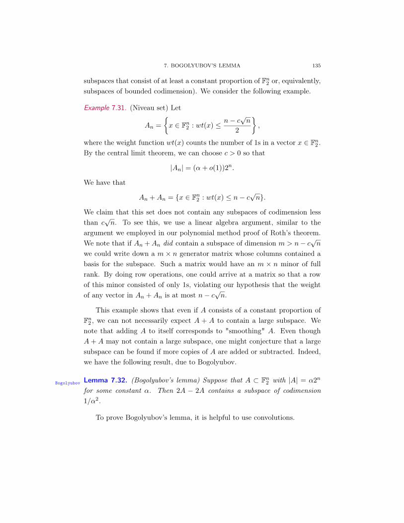
7. BOGOLYUBOV’S LEMMA 135
subspaces that consist of at least a constant proportion of Fn2 or, equivalently,subspaces of bounded codimension). We consider the following example.
Example 7.31. (Niveau set) Let
An =
x ∈ Fn2 : wt(x) ≤ n− c√n
2
,
where the weight function wt(x) counts the number of 1s in a vector x ∈ Fn2 .By the central limit theorem, we can choose c > 0 so that
|An| = (α+ o(1))2n.
We have that
An +An = x ∈ Fn2 : wt(x) ≤ n− c√n.
We claim that this set does not contain any subspaces of codimension lessthan c
√n. To see this, we use a linear algebra argument, similar to the
argument we employed in our polynomial method proof of Roth’s theorem.We note that if An +An did contain a subspace of dimension m > n− c√nwe could write down a m × n generator matrix whose columns contained abasis for the subspace. Such a matrix would have an m × n minor of fullrank. By doing row operations, one could arrive at a matrix so that a rowof this minor consisted of only 1s, violating our hypothesis that the weightof any vector in An +An is at most n− c√n.
This example shows that even if A consists of a constant proportion ofFn2 , we can not necessarily expect A + A to contain a large subspace. Wenote that adding A to itself corresponds to "smoothing" A. Even thoughA+ A may not contain a large subspace, one might conjecture that a largesubspace can be found if more copies of A are added or subtracted. Indeed,we have the following result, due to Bogolyubov.
Lemma 7.32. (Bogolyubov’s lemma) Suppose that A ⊂ Fn2 with |A| = α2nBogolyubov
for some constant α. Then 2A − 2A contains a subspace of codimension1/α2.
To prove Bogolyubov’s lemma, it is helpful to use convolutions.

136 7. STRUCTURE OF SET ADDITION
Definition 7.33. Let Γ be an abelian group. Given f, g : Γ → C, we definethe convolution f ∗ g : Γ→ C by
(f ∗ g)(x) := Ey∈Γ
f(y)g(x− y)
= Ey, z ∈ Γ
y + z = x
f(y)g(z).
The second formulation of the definition of f ∗ g suggests that convolu-tions should be useful for studying sumsets. Indeed, we note that if A,B ⊂ Γ,then the convolution 1A ∗ 1B is supported on A+B. As another example ofhow convolutions correspond to sums, suppose that X is a random variablethat takes values in Γ and that X ∼ µX . This means that for any a ∈ Γ, wehave that
P(X = a) =µX(a)
|Γ| .
Similarly, suppose that Y ∼ µY . Then X + Y ∼ µX ∗ µY .Convolutions interact nicely with the Fourier transform. In particular, we
have the following proposition, which, roughly stated, says that the Fouriertransform takes convolutions to multiplication.
Proposition 7.34. If f, g : Γ→ C, then
f ∗ g = f g. (9) convolution to multiplication
Proof. To prove (convolution to multiplicationconvolution to multiplication9), we must show that for any character γ,
f ∗ g(γ) = f(γ)g(γ).
7. BOGOLYUBOV’S LEMMA 137
This is a fairly routine computation, which we nevertheless write out: forany character γ, we have
f ∗ g(γ) = Ex(f ∗ g)(x)γ(x)
= Ex
Ey, z ∈ Γ
y + z = x
f(y)g(z)γ(y + z)
= E
y,z∈Γf(y)g(z)γ(y + z)
= Ey,z∈Γ
f(y)g(z)γ(y) γ(z)
=
(Eyf(y)γ(y)
)(Ezg(z)γ(z)
)= f(γ)g(γ).
lec22, part 1: FredericKoehler
We now have the technology to prove Bogolyubov’s lemma. First wegive a proof in the finite field setting. Recall that A ⊂ Fn2 , |A| = α2n andwe are trying to show that 2A − 2A contains a subspace of codimension atmost 1/α2.
Remark 7.35. Here we are making an immaterial distinction between A and−A, i.e. choosing to write 2A − 2A instead of 4A, which will matter laterwhen we move to Z/NZ. The reason we look at 4A is because we previouslysaw an example where 2A does not contain any large subspaces (the Niveauset); but by going to 4A we “smooth” the set even more and it turns out wecan now find large subspaces.
Proof of LemmaBogolyubovBogolyubov7.32. Consider f = 1A ∗ 1A ∗ 1−A ∗ 1−A. Observe that
f = 12A12−A = |1A|4. By Fourier inversion
f(x) =∑r∈Fn2
f(r)(−1)r·x.
Observe that if f(x) > 0 then x ∈ 2A− 2A.How can we make f(x) large?
• f(0) = α4 is large, but this term alone is not enough, the otherterms can annihilate this positive contribution.

138 7. STRUCTURE OF SET ADDITION
• We want to avoid x s.t. r ·x = 1 for some r with |1A(r)| large, sincethese give large negative contributions.
Let R = r ∈ Fn2 \ 0 : |1A(r)| > α3/2. By Parseval, there cannot be toomany large coefficients:
|R|α3 <∑r∈Fn2
|1A(r)|2 = E|1A|2 = α
Hence |R| < α−2.Now observe that if x ∈ R⊥, then
f(x) =∑r∈Fn2
|1A(r)|4(−1)r·x
= |1A(0)|4 +∑r∈R|1A(r)|4 +
∑r/∈(R∪0)
|1(r)|4(−1)r·x
≥ α4 + 0− α3∑
r/∈(R∪0)|1A(r)|2
> α4 − α3α = 0
since for r /∈ (R ∪ 0) we know |1(r)| ≤ α3/2, and in the last step we usedParseval (the inequality is strict since we added r = 0 to the sum).
So x ∈ 2A − 2A whenever x ∈ R⊥, which gives the desired subspace ofcodimension |R| < α−2.
We want to do the same proof in Z/nZ but we no longer have subspaces!Instead we will use Bohr sets.
Definition 7.36 (Bohr Sets). Suppose R ⊂ Z/NZ. We call |R| the dimensionand ε the width of the Bohr set,
Bohr(R, ε) =
x ∈ Z/NZ :
∥∥∥rxN
∥∥∥R/Z≤ ε for all r ∈ R
where the norm denotes the distance to Z.
To make the analogy to subspaces in the Fn2 case, we should think of εas close to 0 and then we can think of this as asking that the inner productr · x ≈ 0, similar to defining a subspace by its orthogonal vectors.
However, Bohr sets are less nice than subspaces because they are notclosed under addition; all we know is thatBohr(R, ε)+Bohr(R, ε) ⊂ Bohr(R, 2ε).(And note that growing the radius of the ball by a factor of 2 typically makesthe size exponentially larger in the dimension |R|.)
7. GEOMETRY OF NUMBERS 139
bogolyubov-cyclic Lemma 7.37 (Bogolyubov’s lemma in Z/NZ). Suppose A ⊂ Z/NZ and |A| =αN . Then 2A−2A contains a Bohr set of dimension at most α−2 and width1/4.
Remark 7.38. Note that dimension of a Bohr set corresponds to the codi-mension of a subspace under our analogy, so this lemma is indeed analogousto its Fn2 version.
Proof. This is basically the same proof as the Fn2 version. Let
f = 1A ∗ 1A ∗ 1−A ∗ 1−A
sof = |1A|4.
LetR = r ∈ Z/NZ : |1A(r)| > α3/2.
Observe that if x ∈ Bohr(R, 1/4) then cos(2πrxN ) ≥ 0 since ‖rx/N‖R/Z ≤
1/4. By Parseval
|R|α3 <∑
r∈Z/NZ|1A(r)|2 = E|1A|2 = α.
By Fourier inversion and the fact that f(x) is real-valued
f(x) =∑
r∈Z/NZ|1A(r)|4e2πi(rx/N)
=∑
r∈Z/NZ|1A(r)|4 cos(
2πrx
N)
= |1A(0)|4 +∑r∈R|1A(r)|4 cos(
2πrx
N) +
∑r/∈(R∪0)
|1A(r)|4 cos(2πrx
N)
≥ α4 + 0− α3∑
r/∈R∪0|1A(r)|2
> α4 − α4 = 0
hence x ∈ 2A− 2A.
§7.6 Geometry of numbers
Note that a Bohr set is not the same as an arithmetic progression, so thenext step towards proving Freiman’s theorem is to show that a large Bohrset must contain a large arithmetic progression.

140 7. STRUCTURE OF SET ADDITION
We remind ourselves of the big picture: if a set has small doubling, thenits iterated sums are small by Plunecke-Rusza, Ruzsa’s model lemma showswe can embed a large subset A′ of A into a cyclic group of comparable sizeto A′, Bogolyubov’s lemma tells us that 2A′ − 2A′ contains a large Bohrset, and next we show that the large Bohr set contains a large arithmeticprogression.
Proposition 7.39. A Bohr set of dimension d and width ε in Z/NZ mustcontain a proper generalized arithmetic progression (recall proper means thatall elements that should be distinct are distinct, like a proper parallelipied)of dimension at most d and size at least (ε/d)dN .
To prove this statement we need tools from geometry of numbers. Geom-etry of numbers basically concerns the study of lattices and convex bodieswith application to number theory. Before we start to prove Minkowski’sfundamental theorems, we need to briefly review some basic definitions andproperties of lattices. Proofs of facts here can be found in e.g. any introduc-tory text on algebraic number theory (such as Neukirch’s book).
Definition 7.40. A lattice Λ is a discrete subgroup of Rd.
Obviously integer combinations of any linear independent vectors v1, . . . , vd
generate a lattice that spans Rd. The next proposition asserts that all latticesare of this form.
Proposition 7.41. If a lattice spans Rd, then it has an integral basis v1, v2, . . . , vd
such thatΛ = Zv1 ⊕ · · · ⊕ Zvd.
Example 7.42. Identify C with R2 and let ω be a primitive third root of unity;consider the lattice Λ = Z1+Zω; then we also have Λ = Z(1+ω)+Z(2+ω).This shows that the integral basis is not unique.
Example 7.43. Z1 + Z√
2 ⊂ R is a not an example of a lattice in R becauseit is not discrete.
Definition 7.44. The determinant of a lattice is given by
det(Λ) = |det(v1 · · · vd)|
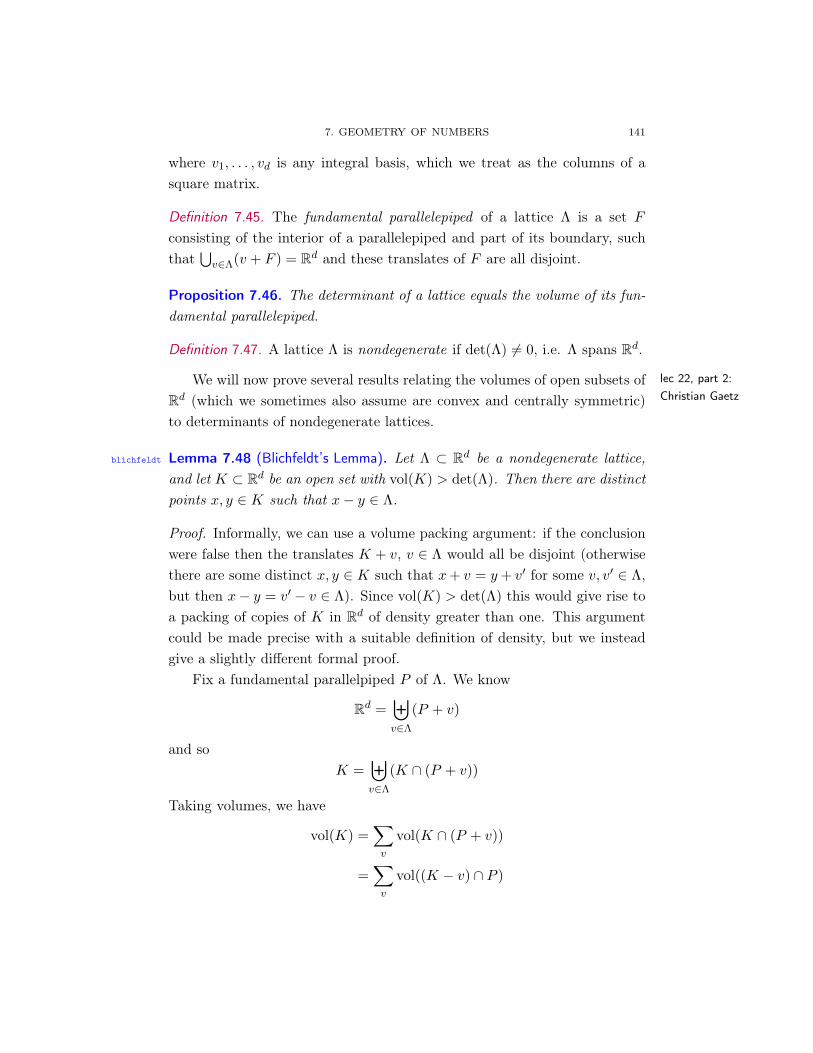
7. GEOMETRY OF NUMBERS 141
where v1, . . . , vd is any integral basis, which we treat as the columns of asquare matrix.
Definition 7.45. The fundamental parallelepiped of a lattice Λ is a set Fconsisting of the interior of a parallelepiped and part of its boundary, suchthat
⋃v∈Λ(v + F ) = Rd and these translates of F are all disjoint.
Proposition 7.46. The determinant of a lattice equals the volume of its fun-damental parallelepiped.
Definition 7.47. A lattice Λ is nondegenerate if det(Λ) 6= 0, i.e. Λ spans Rd.
lec 22, part 2:Christian Gaetz
We will now prove several results relating the volumes of open subsets ofRd (which we sometimes also assume are convex and centrally symmetric)to determinants of nondegenerate lattices.
blichfeldt Lemma 7.48 (Blichfeldt’s Lemma). Let Λ ⊂ Rd be a nondegenerate lattice,and let K ⊂ Rd be an open set with vol(K) > det(Λ). Then there are distinctpoints x, y ∈ K such that x− y ∈ Λ.
Proof. Informally, we can use a volume packing argument: if the conclusionwere false then the translates K + v, v ∈ Λ would all be disjoint (otherwisethere are some distinct x, y ∈ K such that x+ v = y+ v′ for some v, v′ ∈ Λ,but then x− y = v′ − v ∈ Λ). Since vol(K) > det(Λ) this would give rise toa packing of copies of K in Rd of density greater than one. This argumentcould be made precise with a suitable definition of density, but we insteadgive a slightly different formal proof.
Fix a fundamental parallelpiped P of Λ. We know
Rd =⊎v∈Λ
(P + v)
and soK =
⊎v∈Λ
(K ∩ (P + v))
Taking volumes, we have
vol(K) =∑v
vol(K ∩ (P + v))
=∑v
vol((K − v) ∩ P )

142 7. STRUCTURE OF SET ADDITION
But vol(K) > det(Λ) = vol(P ), so some two translates must overlap inP , giving x − v = y − v′ for some x, y ∈ K and distinct v, v′ ∈ Λ, thusx− y = v − v′ 6= 0 ∈ Λ.
As an easy corollary of Blichfeldt’s Lemma, we obtain:
Minkowski1 Theorem 7.49 (Minkowski’s First Theorem). Let Λ be a nondegenerate lat-tice and K a centrally symmetric convex set, both in Rd. Suppose vol(K) >
2d det(Λ), then K contains a nonzero point of Λ.
Proof. By hypothesis, vol(12K) = 2−d vol(K) > det(Λ), so by Lemma
blichfeldtblichfeldt7.48
there exist x, y ∈ K such that x− y ∈ Λ \ 0. Since K is centrally symmetric,we see that −2y ∈ K, and therefore 1
2(2x−2y) = x−y ∈ K by convexity.
open cube Remark 7.50. The constant 2d in TheoremMinkowski1Minkowski17.49 is tight, as can be seen by
taking K to be the interior of a d-cube of side length 2, centered at theorigin, and Λ to be the standard coordinate lattice.
We will not actually need TheoremMinkowski1Minkowski17.49 for our purposes, but rather
a generalization known as Minkowski’s Second Theorem. Although Remarkopen cubeopen cube7.50 shows that the constant 2d cannot be uniformly improved, that exampleis very special: as we scale K we hit lattice points in all directions simul-taneously. In order to state Minkowski’s Second Theorem, we first need tomake some definitions which account more precisely for the shape of K withrespect to Λ.
Given a centrally symmetric convex body K ⊂ Rd, define the i-th suc-cessive minimum λi by
λi := infλ | λK contains i linearly independent elements of Λ
The i-th directional basis vector bi is the unique vector (up to sign and coin-cidences of the λi) such that bi ∈ λiK ∩ Λ and dim spanb1, ..., bi = i.
Intuitively we can think of scaling K by a very small factor λ which wethen let grow slowly. Then λ1 is the first value of λ at which λK hits anonzero point x of Λ, and b1 points in the direction of x. We then continuescaling λ until λK hits more points of Λ, except that we require these pointsto be in genuinely new directions.
Minkowski2 Theorem 7.51 (Minkowski’s Second Theorem). Let K be a centrally symmet-ric convex body and Λ a nondegenerate lattice, both in Rd, and let λ1, ..., λd

7. GEOMETRY OF NUMBERS 143
be the successive minima. Then
λ1λ2 · · ·λd · vol(K) ≤ 2d · det(Λ)
Remark 7.52. This is a generalization of TheoremMinkowski1Minkowski17.49. We have (λ1K
)∩Λ =
0, and so by TheoremMinkowski1Minkowski17.49, we must have vol(λ1K) = λd1 vol(K) ≤
2d vol(Λ). TheoremMinkowski2Minkowski27.51 allows us to replace the constant λd1 with the pos-
sibly bigger constant λ1λ2 · · ·λd.
Proof. This proof is somewhat unintuitive. The idea is to grow K until wehit a point of Λ, and then continue growing, but only in the complementarydirection. However rigorously carrying out this procedure is very tricky.
It suffices to prove the theorem in the case where K is open. Fix adirectional basis b1, ..., bd; the fact that K is open implies that (λiK) ∩ Λ ⊂spanb1, ..., bi−1. For j = 1, ..., d, we define maps φj : K → K by sendinga point x ∈ K to the center of mass of the (j − 1)-dimensional slice of Kwhich contains x and is parallel to b1, ..., bj−1. (We will see later that theexact "center of mass" property is not essential to the proof; we simply wantall points in a hyperplane slice of K to be sent to a unique point also withinK that respects K’s symmetry). In particular, φ1 is the identity function.We also define a function φ : K → Rd by
φ(x) =d∑j=1
(λj − λj−1)φj(x)/2
where by convention we let λ0 = 0. We will see that φ(K) has volumeλ1λ2 · · ·λd/2d and that φ(K) contains no lattice points, but this will take abit more work.
lec23: SaraneshPrembabu/BenjaminGunby
φ is intended to encapsulate this process of growing first in one direction(given by the first term of the sum), then in the second direction (givenby the second term of the sum), et cetera. Naively trying to grow in alldirections in an ‘affine’ way doesn’t work properly.
For x ∈ Rd, let xi be its entries in the basis (bi), so that x =d∑i=1
xibi.
Note thatφj(x) =
∑i<j
cj,i(xj , . . . , xd)bi +∑i≥j
xibi
for some continuous functions cj,i.
144 7. STRUCTURE OF SET ADDITION
Therefore,
φ(x) =d∑i=1
(λixi/2 + ψi(xi+1, . . . , xd))bi
for some continuous functions ψi. So the Jacobian J(φ) = ∂φ(x)∂xj
is uppertriangular with diagonal entries λ1/2, . . . , λd/2. This implies that
vol(φ(K)) = λ1 · · ·λdvol(K)/2d.
which is conveniently the left hand side of the inequality of Minkowski’sSecond Theorem λ1 · · ·λdvol(K)/2d < det Λ which we seek to prove..
We return to the proof of Minkowski’s Second Theorem.For any distinct points x =
∑xibi, y =
∑yibi in K, let k be the
largest index such that xk 6= yk. Then φi(x) agrees with φi(y) for all i > k.Therefore,
φ(x)− φ(y) =
d∑j=1
(λj − λj−1)
(φj(x)− φj(y)
2
)
=
k∑j=1
(λj − λj−1)
(φj(x)− φj(y)
2
)
∈k∑j=1
(λj − λj−1)K
= λkK.
The third line is due to convexity and symmetry of K.The coefficient of bk in (φ(x) − φ(y)) is λk
(xk−yk2
)6= 0. In particular,
this means (φ(x) − φ(y)) lies outside the span of b1, b2, . . . bk−1 but insidethe interior of λkK (which is an open set that does not include bk); thus itis not a lattice vector.
Since φ(K) contains no two points separated by a nonzero lattice vector,it must have volume less than or equal to det(Λ) (by Blichfeldt’s Lemma).Combining this with the Jacobian volume relation, we haveλ1 · · ·λdvol(K)/2d <
det Λ and the theorem is proved.
Remark 7.53. We have a reverse inequality 2d
d! det Λ ≤ λ1 · · ·λdvolK.
Proof. The cross polytope with vertices ± b1λ1, . . . ,± bd
λd∈ K has volume
2d
d!det Λλ1···λd and is contained in the closure of K.
7. GEOMETRY OF NUMBERS 145
We now return to the proof that every Bohr set contains a large gener-alized arithmetic progression of low dimension. Since Bogolyubov’s theoremalready guarantees the existence of a suitable Bohr set, the proposition wewill prove will ultimately make it possible to find a large GAP as needed forFreiman’s theorem.
BohrGAPProp Proposition 7.54. Let R ⊆ Z/nZ with N prime, 0 < ε < 1, |R| = d. ThenBohr(R, ε) contains a proper generalized arithmetic progression of dimensionat most d and size
(εd
)dN .
Proof. Let R = r1, . . . , rd, and let r = (r1, . . . , rd) ∈ Zd. Λ := N ·Zd+rZ =
N ·Zd⊕0, 1, . . . , (n−1)·r is a lattice, and is a direct sum as N is prime. Λ
is the lattice formed by adding N multiples of vector r to each lattice pointof the rectangular lattice Λ0 = N · Zd. Because of this, det Λ = Nd−1 (eachunit cell of Λ0 contains N points and has volume Nd, so the volume of aunit cell of Λ must be N times less).
Let K = x ∈ Rd : ||x||∞ := max|x1|, . . . , |xd| < 1 be the interiorof a hypercube centred at the origin with side lengths 2 . Further let λ1 ≤· · · ≤ λd be the successive minima of K with respect to Λ, and b1, . . . , bd
be a corresponding directional basis (as defined in our proof of Minkowski’ssecond theorem). Note that by the definition ofK, ||bi||∞ = λi ( where ||bi||∞refers to maxj((bi)j) when bi is written as a vector ((bi)1, (bi)2, . . . (bi)d) inthe original basis). Since bi ∈ Λ, ∃xi ∈ Z/NZ such that bi ≡ xir (mod N).
We claim that the generalized arithmetic progression
P :=
`1x1 + · · ·+ `dxd : 0 ≤ `i <
εN
λid
is proper and contained in Bohr(R, ε).
Indeed, ∣∣∣∣∣∣xirjN
∣∣∣∣∣∣R/Z
=
∣∣∣∣∣∣∣∣(bi)jN
∣∣∣∣∣∣∣∣R/Z≤∣∣∣∣(bi)jN
∣∣∣∣ ≤ λiN.
Thus ∀p := `1x1 + · · ·+ `dxd ∈ P ,∣∣∣∣∣∣prjN
∣∣∣∣∣∣R/Z≤
d∑i=1
`i
∣∣∣∣∣∣xirjN
∣∣∣∣∣∣R/Z≤
d∑i=1
(εN
λid
)(λiN
)= ε.
Hence p ∈ Bohr(R, ε).We now prove P is proper. Suppose ` =
∑`ixi and `′ =
∑`′ixi such
that ` ≡ `′ (mod N). We know that 0 ≤ `i, `′i < εNλid
.

146 7. STRUCTURE OF SET ADDITION
Let b :=d∑i=1
(`i−`′i)bi ≡ (`−`′)r ≡ 0 (mod N) (To clarify notation, note
that bi is not the ith component of b in the original basis, but rather is theith basis vector). Then
||b||∞ ≤d∑i=1
|`i − `′i|||bi||∞
≤d∑i=1
εN
λidλi
≤ εN< N
Thus b = 0. Since bi is a basis andd∑i=1
(`i − `′i)bi = b = 0, `i = `′i. Thus P is
proper.It is clear that dim(P ) ≤ d. Its size is
d∏i=1
(εN
λid
)=( εd
)d Nd
λ1 · · ·λd
≥( εd
)d Ndvol(K)
2d det Λ
=( εd
)dN,
where the inequality is by Minkowski’s Second Theorem and we use the factthat vol(K) = 2d and det Λ = Nd−1. This completes the proof.
§7.7 Proof of Freiman’s Theorem
Putting the results of the previous two sections together, we have proventhe following.
2aminus2a Proposition 7.55. Let A ⊆ Z/NZ with N prime and |A| = αN . Then2A − 2A contains a proper generalized arithmetic progression of dimensiond ≤ 1
α2 and size at least(
14d
)dN .
Proof. By Bogolyubov’s Lemma, 2A− 2A contains a Bohr set of dimensiond ≤ 1
α2 and width 14 . By Proposition
BohrGAPPropBohrGAPProp7.54 with ε = 1
4 , we get a generalizedarithmetic progression of the desired size.
Proof of Freiman’s Theorem. The proof outline is as follows.

7. PROOF OF FREIMAN’S THEOREM 147
(1) By the Ruzsa’s model lemma, a large subset of A is Freiman-8-isomorphic to a large subset B ⊂ Z/NZ, with N prime.
(2) 2B− 2B contains a large generalized arithmetic progression by theprevious proposition, so 2A− 2A does also.
(3) By the Rusza Covering Lemma, A is covered by a small number oftranslates of this generalized arithmetic progression.
We now give the details. Cite theoremnumbers–done.Cite theoremnumbers–done.(1) By Corollary
8isomorphism8isomorphism7.29, there exists a prime N ≤ 2K16|A| and A′ ⊂ A,
|A′| ≤ |A|8 such that A′ is Freiman-8-isomorphic to some B ⊂ Z/NZ.(2) By Proposition
2aminus2a2aminus2a7.55 with α = |B|
N ≥ |A|8N ≥ 1
16K16 , we see that2B − 2B contains a proper generalized arithmetic progression ofdimension d ≤ 256K32 and size at least
(14d
)dN .
Because B is Freiman-8-isomorphic to A′, 2B − 2B is Freiman-2-isomorphic to 2A′−2A′ (an easy exercise, as a map that preservesinformation about length-8 sums for A′ necessarily preserves length-2 sums of 2A′ − 2A′). Thus the generalized arithmetic progressionin 2B − 2B is sent by our Freiman-2-isomorphism to a subset of2A−2A, which must be a proper generalized arithmetic progression,call it P .
(3) Since P ⊂ 2A− 2A, P +A ⊂ 3A− 2A. Therefore,
|P +A| ≤ |3A− 2A| ≤ K5|A|
by Plünnecke-Rusza. Since N ≥ |A′| ≥ |A|8 and |P | >(
14d
)dN , we
find that |P +A| ≤ K ′|P |, where K ′ = 8(4d)dK5.By the Ruzsa covering lemma, A ⊆ X+P −P for some X ⊂ A
with |X| ≤ K ′. X +P −P is contained in a generalized arithmeticprogression by considering
X ⊂ ∑x∈X
axx : ax ∈ 0, 1.
The dimension of this arithmetic progression is at most d + K ′,and its size is at most 2d+K′ |P | ≤ 2d+K′ |2A − 2A| ≤ 2d+K′K4|A|,finishing the proof.
lec24 (need to addreferences): VisheshJain
Recall that Freiman’s theorem states that if A ⊂ Z and |A + A| ≤K|A|, then A is contained in a generalized arithmetic progression (GAP) ofdimension at most d(K) and size at most f(K)|A|. What can we say about
148 7. STRUCTURE OF SET ADDITION
the growth of d(K) and f(K) as functions of K? An upper bound of d(K) =
2(2K)O(1)and f(K) = 22(2K)O(1)
can be deduced by keeping track of constantsin the proof of Freiman’s theorem presented earlier. On the other hand, ifA is a subset of the integers of size m with no additive relations whatsoever,then K = m+1
2 , any GAP containing A has dimension at least m−1 and thesize of the GAP is at least 2m−1. This gives lower bounds on d(K) and f(K)
that are exponentially better than the upper bounds mentioned above. Itis conjectured that the optimal upper bounds for Freiman’s theorem shouldmatch these lower bounds (up to constant factors). In the sequel, for ease ofnotation, we will use KO(1) to refer to (2K)O(1).
OptimalFreiman Conjecture 7.56 (Optimal bounds for Freiman’s Theorem). In the statementof Freiman’s theorem, it is possible to take d(K) = O(K) and f(K) = 2O(K).
Let us briefly summarize the progress on this conjecture. In step (3) ofthe proof of Freiman’s theorem provided above, if we replace the applicationof Ruzsa’s Covering Lemma by Chang’s Covering Lemma (TO DO: Addreference), one can instead obtain the exponentially better bounds d(K) =
KO(1) and f(K) = 2KO(1) . The best known bounds on Freiman’s theorem
are due to Sanders (TO DO: Add reference), who improved the constants inBogulyubov’s Lemma to show that one can take d(K) = K(logK)O(1) andf(K) = 2K(logK)O(1) .
For Fn2 (and more generally, for Fnp for all primes p), the analog of Conjec-ture
OptimalFreimanOptimalFreiman7.56 has already been settled (TO DO: Add reference). More precisely,
if A ⊆ Fn2 and |A + A| ≤ K|A|, then |〈A〉| ≤ f(K)|A| where the exact op-timal f(K) is known. Asymptotically, f(K) = KO(1)4K . However, one canask if there always exists a “small” (size KO(1)|A|) subspace of Fn2 containinga “large” fraction (K−O(1)) of A. This is the content of one of the mostimportant open problems in additive combinatorics.
PFR-conjecture Conjecture 7.57 (Polynomial Freiman-Ruzsa Conjecture for Fn2 ). Let A ⊆ Fn2such that |A + A| ≤ K|A|. Then, there exists a subspace V ≤ Fn2 such that|V | ≤ KO(1)|A| and |V ∩A| ≥ K−O(1)|A|.
Remark 7.58. By an application of Ruzsa’s covering lemma, which we leaveas an exercise to the reader, this is equivalent to saying that A can be coveredby KO(1) many translates of V .

7. PROOF OF FREIMAN’S THEOREM 149
The best known result towards ConjecturePFR-conjecturePFR-conjecture7.57 is due to Sanders (TO
DO: Add reference) who proved it with quasipolynomial bounds instead ofpolynomial bounds i.e. i.e. bounds of the form e(logK)O(1) instead of eO(logK).
Part of the reason that the Polynomial Freiman-Ruzsa Conjecture is soattractive is that it admits several different equivalent formulations. Here isone such statement:
equiv-PFR-conjecture Conjecture 7.59 (Equivalent formulation of ConjecturePFR-conjecturePFR-conjecture7.57). If f : Fn2 → Fn2
is such that |f(x + y) − f(x) − f(y) : x, y ∈ Fn2| ≤ K, then there exists alinear map g : Fn2 → Fn2 such that S = im(f − g) = f(x) − g(x) : x ∈ Fn2satisfies |S| = KO(1).
Remark 7.60. Proving the above conjecture with |S| ≤ 2K is very easy. Sim-ply pick g to agree with f on an arbitrarily chosen basis. Then S is containedin the linear span (over F2) of at mostK vectors f(x+y)−f(x)−f(y) : x, y ∈Fn2 and hence, |S| ≤ 2K .
The analog of ConjecturePFR-conjecturePFR-conjecture7.57 for the integers has also attracted a lot of
interest.
PFR-conj-integers Conjecture 7.61 (Polynomial Freiman-Ruzsa Conjecture for Z). If A ⊂ Z sat-isfies |A+A| ≤ K|A|, then there exists a convex progression P := a0+n1a1+
· · · + ndad : (n1, . . . , nd) ∈ Zd ∩ B, where B ⊂ Rd is some convex body inRd and a0, . . . ad ∈ Z, such that d = O(1 + logK), |B ∩ Zd| ≤ KO(1)|A|and|P ∩A| ≥ K−O(1)|A|.
As before, this is equivalent to saying that A can be covered by KO(1)
many translates of P .Recall that in the proof of Freiman’s theorem, the application of Bogu-
lyubov’s lemma formed a key step. We also mentioned above that a resultof Sanders improving the constants in Bogulyubov’s lemma leads to thebest known bounds for Freiman’s theorem. The situation for the Polyno-mial Freiman-Ruzsa conjectures is similar in the sense that the best knownresults have been obtained via improvements for Bogulyubov’s lemma. Infact, the following conjectured strengthenings of Bogolyubov’s lemma wouldimply the corresponding Polynomial Freiman-Ruzsa conjecture.
PBR-conjecture-F2 Conjecture 7.62 (Polynomial Bogulyubov-Ruzsa Conjecture for Fn2 ). If A ⊆ Fn2with |A| = α2n, then 2A− 2A contains a subspace of codimension O(log 1
α).
150 7. STRUCTURE OF SET ADDITION
The best known result here is also due to Sanders, who proved the con-jecture with (log 1
α)O(1) instead of O(log 1α).
Remark 7.63. Proving the above conjecture with 2A−2A replaced by `A−`Afor any ` would still imply Conjecture
PFR-conjecturePFR-conjecture7.57.
PBR-conjecture-Zmodn Conjecture 7.64 (Polynomial Bogulyubov-Ruzsa Conjecture for Z/NZ). Let Nbe a prime number. If A ⊂ Z/NZ with |A| = αN , then 2A− 2A contains aproper convex progression of dimension O(log 1
α) and size at least αO(1)N
While the Polynomial Bogulybov-Ruzsa conjectures imply the corre-sponding Polynomial Freiman-Ruzsa conjectures, it is unknown whether theconverse is true.
§7.8 Additive Energy and the Balog-Szemerédi-GowersTheorem
The theme of Freiman’s theorem is to express in multiple ways the factthat a set has a lot of additive structure. We now look at yet another wayof expressing (the presence of) additive structure in a set.
AdditiveEnergyDefn Definition 7.65. Let Γ be an abelian group. For finite subsets A,B ⊆ Γ, theadditive energy betweenA andB is defined to be E(A,B) := |(a1, a2, b1, b2) ∈A×A×B ×B : a1 + b1 = a2 + b2|.
A very useful equivalent way of viewing the additive energy is the fol-lowing: let rA,B(n) := |(a, b) ∈ A× B : n = a+ b| denote the number ofways the element n can be represented as a sum a + b with a ∈ A, b ∈ B.Then, it is immediately seen that E(A,B) =
∑n∈Γ rA,B(n)2.
We will use E(A) to denote E(A,A). Note that E(A) ≥ |A|2 since wehave |A|2 “trivial” quadruples of the form (a1, a2, a2, a1) with a1, a2 ∈ A.We also have the trivial upper bound E(A) ≤ |A|3 since specifying threeelements of any valid quadruple uniquely determines the fourth element.Hence, the additive energy E(A) always ranges between |A|2 and |A|3. Asexamples, note that if Γ = Z and A = [N ], then E(A) = Θ(N3) whereas if Ahas no additive structure, then E(A) = |A|2. In general, we should think ofadditive energy “close to cubic” as a sign of additive structure. Since we havealso seen that “small doubling” is a sign of additive structure, it is naturalto ask how, if at all, the conditions |A + A| ≤ K|A| and E(A) ≥ c|A|3 arerelated.
7. ADDITIVE ENERGY AND THE BALOG-SZEMERÉDI-GOWERS THEOREM 151
SmlDoublingLargeAddEnergy Proposition 7.66 (Small doubling implies large additive energy). Let A be a fi-nite subset of an abelian group Γ. If |A+A| ≤ K|A|, then E(A) ≥ |A|3K .
Proof. Let r(x) = |(a, a′) ∈ A×A : a+a′ = x|. Then, as observed earlier,E(A) =
∑x r(x)2. Note that
∑x r(x) = |A|2 since every pair (a, a′) is
accounted for exactly once (in the summand r(a+a′)) on the left hand side.Note also that r is supported on A + A. Now, an application of Cauchy-Schwarz shows that
|A+A|.E(A) = |A+A|(∑
x
r(x)2
)
≥(∑
x
r(x)
)2
= |A|4
which shows that E(A) ≥ |A|4|A+A| ≥
|A|3K – the last inequality following
from the assumption that |A+A| ≤ K|A|.
However, the reverse implication is not true. Indeed, consider Γ = Z andA = [m] ∪ m additional elements introducing no new additive relations.Then, E(A) ≥ E([m]) = Θ(|A|3) whereas |A+A| ≥ m2 ≥ m
2 |A|. Essentially,a set can have large additive energy if a “large” fraction of it has additivestructure whereas the small doubling condition really takes into account theset as a whole. Therefore, for some sort of converse to Proposition
SmlDoublingLargeAddEnergySmlDoublingLargeAddEnergy7.66, it is
natural to look for statements about dense subsets of sets with large additiveenergy. The Balog-Szemerédi-Gowers theorem provides such a converse byshowing that any set with large additive energy contains a dense subset withsmall doubling.
BSG-Thm Theorem 7.67 (Balog-Szemerédi-Gowers (BSG)). Let Γ be an abelian groupand let A,B ⊆ Γ with |A| = |B| = n. If E(A,B) ≥ n3
K , then there existA′ ⊆ A,B′ ⊆ B with |A′|, |B′| ≥ K−O(1)n such that |A′ +B′| ≤ KO(1)n.
Remark 7.68. Setting A = B in the above theorem gives us subsets A′, A′′ ofA such that |A′|, |A′′| ≥ K−O(1)n and |A′ + A′′| ≤ KO(1)n. Then, Ruzsa’s

152 7. STRUCTURE OF SET ADDITION
triangle inequality shows that
K−O(1)n.|A′ +A′| ≤ |A′′|.|A′ +A′|≤ |A′ +A′′|.|A′ +A′′|≤ KO(1)n2
which shows that |A′ + A′| ≤ KO(1)n i.e. A′ is a dense subset of A withsmall doubling.
We will deduce the BSG theorem from the following graph analog, whichwill be proved via the technique of dependent random choice. Given a bipar-tite graph G between vertex sets A and B, defined A+GB := a+b : (a, b) ∈A×B is an edge of G.
GraphBSG-Thm Theorem 7.69 (Graph BSG). Let Γ be an abelian group, and let A,B ⊆ Γ
with |A| = |B| = n. Let G be a bipartite graph between the vertex sets A andB such that G has at least n2
K edges. If |A +G B| ≤ Kn, then there existA′ ⊆ A,B′ ⊆ B with |A′|, |B′| ≥ K−O(1)n such that |A′ +B′| ≤ KO(1)n.
Before giving the proof of this theorem, let us show how it implies theBSG theorem.
GraphBSGimpliesBSG Lemma 7.70. The Graph BSG theorem (TheoremGraphBSG-ThmGraphBSG-Thm7.69) implies the BSG
theorem (TheoremBSG-ThmBSG-Thm7.67).
Proof. Suppose |A| = |B| = n with E(A,B) ≥ n3
K . As before, let r(x) =
|(a, b) ∈ A × B : a + b = x| and let S = x ∈ A + B : r(x) ≥ n2K
denote the set of “popular sums”. Note that by definition,∑
x/∈S r(x)2 ≤maxx/∈S r(x) ×∑x/∈S r(x) ≤ n
2K × n2, where the last inequality uses thetrivial bound
∑x/∈S r(x) ≤∑x r(x) = |A|.|B| = n2. Then:
n3
K≤ E(A,B)
=∑x
r(x)2
=∑x∈S
r(x)2 +∑x/∈S
r(x)2
≤∑x∈S
r(x)2 +n3
2K

7. ADDITIVE ENERGY AND THE BALOG-SZEMERÉDI-GOWERS THEOREM 153
which shows thatn3
2K≤∑x∈S
r(x)2 ≤ n∑x∈S
r(x)
and hence,∑
x∈S r(x) ≥ n2
2K . Let G be the bipartite graph between vertexsets A and B where (a, b) ∈ A×B is an edge in G if and only if a+b ∈ S. Bythe previous paragraph, the number of edges in G equals
∑x∈S r(x) ≥ n2
2K .Moreover, since |A+GB| denotes the number of “popular sums”, each popularsum is associated with at least n
2K many distinct pairs (a, b) and since thereare only n2 many such pairs (a, b), it follows that n
2K .|A +G B| ≤ n2 i.e.|A +G B| ≤ 2Kn. Since G satisfies the hypotheses of Theorem
GraphBSG-ThmGraphBSG-Thm7.69 with
K replaced by 2K, we can apply the Graph BSG theorem to finish theproof.
Lec25: DhroovaAiylam
We now give a proof of the Graph BSG theorem via a series of lemmas.
PathsOfLength2 Lemma 7.71 (Paths of Length 2). Suppose G is a bipartite graph betweenvertex sets A and B which has at least δ|A||B| edges, and let ε > 0 begiven. Then there exists U ⊂ A with |U | ≥ δ|A|/2 such that between at least(1 − ε)|U |2 ordered pairs (u, u′) ∈ U × U , there are at least εδ2|B|/2 manypaths of length 2 between u and u′.
The proof uses dependent random choice to pick U ; in particular, we willpick a random vertex in B random and take U to be its neighborhood. Theidea is that if u, u′ ∈ U have few common neighbors in B, then it is unlikelywe chose them.
U
A B
v
Proof. Choose v ∼ Unif(B) and let U = N(v). By convexity,
E[|U |2] ≥ (E[|U |])2 = δ2|A|2.
154 7. STRUCTURE OF SET ADDITION
We say a pair (a, a′) ∈ A2 is bad if codeg(a, , a′) < εδ2|B|/2. For (a, a′) afixed bad pair, we have
P(a, a′ ∈ U) = P(v ∈ N(a) ∩N(a′)) <1
2εδ2.
Let Z be the random variable which counts the number of bad pairs inU × U ; from the above and linearity of expectation, E[Z] ≤ εδ2|A|2/2. Itfollows that
E[|U |2 − Z
ε
]≥ δ2|A|2 − 1
2δ2|A|2 ≥ 1
2δ2|A|2.
Thus for some choice of v ∈ B we have |U |2 − Z/ε ≥ δ2|A|2/2. In this case,|U |2 ≥ δ2|A|2/2 so that |U | ≥ δ|A|/2; moreover, Z ≤ ε|U |2 so that at mostε-fraction of pairs in U are bad. Equivalently, there are at (1−ε)|U |2 orderedpairs (u, u′)×U ×U which have at least εδ2|B|/2 paths of length 2 betweenthem.
PathsOfLength3 Lemma 7.72 (Paths of Length 3). For 0 < δ < 1, let G be a bipartite graphbetween vertex sets A and B with at least δ|A||B| edges. Then there existA′ ⊂ A and B′ ⊂ B, where |A′| ≥ cδ|A| and |B′| ≥ cδ|B| for some fixedsmall constant c, such that every pair (a, b) ∈ A′×B′ is connected by at leastδO(1)|A||B| paths of length 3.
Proof Sketch. Recall a useful trick from Chapterch:extremal-graph-theorych:extremal-graph-theory2: in a graph with large
average degree, there is a large subset of vertices with large minimum degree.
(1) Remove vertices in A which have degree less thant δ|B|/2; byLemma
lem:avgtomindeglem:avgtomindeg2.17 we incur at most constant factor shrinkage.
(2) Apply LemmaPathsOfLength2PathsOfLength27.71 to find U ⊂ A, which has |U | ≥ δ|A| and almost
all pairs in U have codegree at least δ−O(1)|B|.(3) Remove vertices in U which are in many bad pairs, yielding A′ with|A′| ≥ |U |/2.
(4) Now every vertex in A′ has degree at least δ|B|/2 by (1), so thereexists B′ ⊂ B with size at least δ|B|/4 such that every vertex in B′
has at least δ|A′|/4 neighbors in A′.

7. ADDITIVE ENERGY AND THE BALOG-SZEMERÉDI-GOWERS THEOREM 155
U
A B
B′
b
A′
To see why this choice of A′, B′ should work, observe that for all a ∈ A′ andb ∈ B′, b is adjacent to a large fraction of the vertices a′ ∈ A, and almost allsuch a′ have large codegree with a.
We are now ready to prove the Graph BSG theorem (TheoremGraphBSG-ThmGraphBSG-Thm7.69).
Proof. By LemmaPathsOfLength3PathsOfLength37.72, there exist A′ ⊂ A and B′ ⊂ B, |A′|, |B′| ≥ K−O(1)n,
such that for all a ∈ A′ and b ∈ B′, there are at least K−O(1)n2 many pathsof length 3 between a and b. We claim that |A′ +B′| ≤ KO(1)n. Indeed, forall a′ ∈ A′ and b′ ∈ B′, there exist K−O(1)n2 many (u, v) ∈ A×B such thata+ v, v + u, u+ b ∈ A+G B. Since
a+ b = (a+ v)− (v + u) + (u+ b)
every element of A′+B′ can be written as x− y+ z, x, y, z ∈ A+G B, in atleast K−O(1)n2 many ways. Thus
K−O(1)n2|A′ +B′| ≤ |A+G B|3 ≤ K3n3
so that |A′ +B′| ≤ KO(1)n as desired.

CHAPTER 8
The Sum-Product Problem
Just as we defined the sumset A + B = a + b : a ∈ A, b ∈ B, we candefine A ·B = ab : a ∈ A, b ∈ B.
ESConjecture Conjecture 8.1 (Erdös-Szemerédi). For all A ⊂ R, max|A + A|, |A · A| ≥|A|2−o(1).
The following example shows that the o(1) term is necessary in the ex-ponent of the RHS.
Example 8.2. Let A = [N ]; clearly |A + A| = 2N − 1. On the other hand,|A ·A| (the so-called Erdös multiplication table problem) is harder to bound.Using techniques from analytic number theory, Ford was able to give theprecise estimate
|A ·A| = Θ
(N2
(logN)δ(log logN)3/2
)
where δ = 1 − (1 + log log 2)/ log 2 ≈ 0.086. However, there is a more ele-mentary way to see that |A ·A| = o(N2).
Indeed, by the Hardy-Ramanujan theorem, all but o(N) of the integersless than or equal to N have (1 + o(1)) log logN prime factors (countingmultiplicity). Thus all but at most o(N2) of the products ab, a, b ≤ N , have(2 + o(1)) log logN prime factors. Yet by Hardy-Ramanjuan once more, allbut o(N2) of the integers less than or equal to N2 have (1+o(1)) log logN2 =
(1 + o(1)) log logN prime factors and so cannot appear in the multiplicationtable.
To furnish a lower bound, we consider integers n ≤ N2 of the form pm,where p is a prime in (N2/3, N ] and m ≤ N . By Prime Number Theorem,the number of choices for (p,m) is at least (1 + o(1))N2/ logN . On theother hand, every such n has at most 2 such representations since n ≤ N2
157
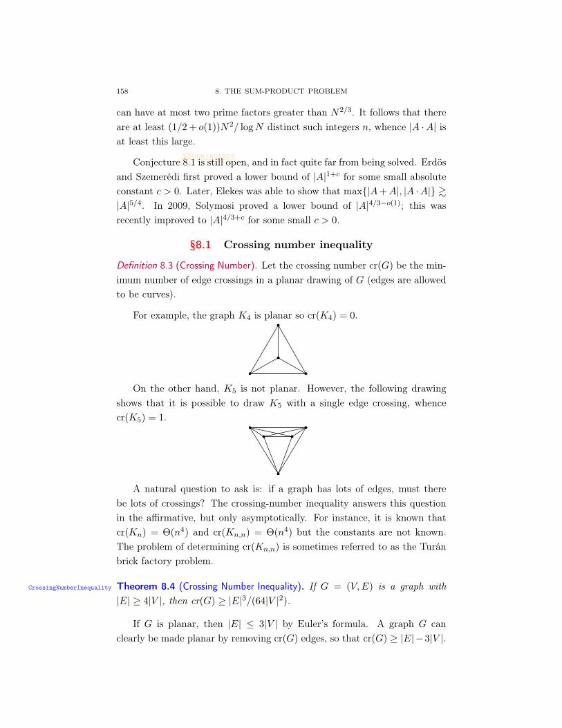
158 8. THE SUM-PRODUCT PROBLEM
can have at most two prime factors greater than N2/3. It follows that thereare at least (1/2 + o(1))N2/ logN distinct such integers n, whence |A ·A| isat least this large.
ConjectureESConjectureESConjecture8.1 is still open, and in fact quite far from being solved. Erdös
and Szemerédi first proved a lower bound of |A|1+c for some small absoluteconstant c > 0. Later, Elekes was able to show that max|A+A|, |A ·A| &|A|5/4. In 2009, Solymosi proved a lower bound of |A|4/3−o(1); this wasrecently improved to |A|4/3+c for some small c > 0.
§8.1 Crossing number inequality
Definition 8.3 (Crossing Number). Let the crossing number cr(G) be the min-imum number of edge crossings in a planar drawing of G (edges are allowedto be curves).
For example, the graph K4 is planar so cr(K4) = 0.
On the other hand, K5 is not planar. However, the following drawingshows that it is possible to draw K5 with a single edge crossing, whencecr(K5) = 1.
A natural question to ask is: if a graph has lots of edges, must therebe lots of crossings? The crossing-number inequality answers this questionin the affirmative, but only asymptotically. For instance, it is known thatcr(Kn) = Θ(n4) and cr(Kn,n) = Θ(n4) but the constants are not known.The problem of determining cr(Kn,n) is sometimes referred to as the Turánbrick factory problem.
CrossingNumberInequality Theorem 8.4 (Crossing Number Inequality). If G = (V,E) is a graph with|E| ≥ 4|V |, then cr(G) ≥ |E|3/(64|V |2).
If G is planar, then |E| ≤ 3|V | by Euler’s formula. A graph G canclearly be made planar by removing cr(G) edges, so that cr(G) ≥ |E|−3|V |.

8. SZEMERÉDI-TROTTER AND INCIDENCE GEOMETRY 159
This bound is not quite good enough – for dense graphs the crossing numberinequality gives a lower bound which is quadratic in |E| – but it is usefulnonetheless.
Proof. Fix G with |E| ≥ 4|V |, and let 0 < p ≤ 1 be a value which we choosein the sequel. Pick V ′ ⊂ V by including each vertex of V independently withprobability p, and let G′ = (V ′, E′) denote the induced subgraph. As beforewe have cr(G′) ≥ |E′| − 3|V ′|; we note that E[|V ′|] = p|V |, E[|E′|] = p2|E|.Moreover, E[cr(G′)] ≤ p4cr(G) by reusing the optimal drawing of G; a cross-ing occurs in G′ if and only if each of the four vertices of its edges is includedin V ′, which has probability p4, whence the claim follows from linearity. Weconclude that
p4cr(G) ≥ E[cr(G′)] ≥ E[|E′|]− 3E[|V ′|] = p2|E| − 3p|V |
i.e. cr(G) ≥ p−2|E| − 3p−3|V |. The result now follows from putting p =
4|V |/|E| ≤ 1.
Lec26: Paxton Turner
§8.2 Szemerédi-Trotter and Incidence Geometry
Methods from geometry, first used by Elekes [13], have obtained resultson the sum-product problem. First we present a motivating example thatuses related techniques on the unit distance problem.
Theorem 8.5. A set of n points in the real plane R2 make at most O(n4/3)
unit length distances.
This is an old problem of Erdős [14], and the conjectured exponent is1 + o(1). Somewhat surprisingly, the exponent 4
3 is the best known and wasobtained by Spencer, Szemerédi, and Trotter [48].
Proof. First remove all points that are involved in at most 2 unit distances,and call the remaining set S. Define a graph G whose vertices are the pointsof S. For all p ∈ S, draw a circle Cp of radius 1 about p. The circle Cpis divided into arcs by the points of Cp ∩ S, so let the edges of G be arcsconnecting consecutive points on the circle. Each pair of circles can cross atmost twice, so the number of crossings in G is at most n2. By the crossing

160 8. THE SUM-PRODUCT PROBLEM
number inequality, TheoremCrossingNumberInequalityCrossingNumberInequality8.4, we get n2 & m3
n2 . Since each edge representsa unit distance, this proves the theorem.
Definition 8.6 (Incidences). Let P ⊂ R be a set of points and L ⊂ R be a setof lines. Then the set of incidences is defined to be
I(P,L) = (p, `) ∈ P × L : p ∈ `.
The Szemerédi-Trotter Theorem tells us how large the set of incidencescan be.
Sze-Trot Theorem 8.7 (Szemerédi-Trotter Theorem). If P ⊂ R is a set of points, andL ⊂ RR is a set of lines, then
I(P,L) = O(|P |2/3|L|2/3 + |P |+ |L|)
Note that P and L play symmetric roles in this inequality. Moreover thistheorem is tight if we let P be a 2n2/3 × n1/3 grid and let L be the set oflines y = mx+ b where 1 < m < n1/3 and 1 ≤ b ≤ n1/3. Here |P | |L| nand |I(P,L)| n4/3. The proof shows that the exponent 4
3 is morally thesame as that obtained for the unit distance problem.
Proof. Remove the lines L that have no points in P . Define a graph G whosepoints are P and whose edges are consecutive points on the lines L (here weremove any trailing rays). The number of edges is |I(P,L)| − |L|. Trivially,the number of crossings is at most
(|L|2
). So if |I(P,L)| − |L| ≥ 4|P |, by the
crossing number inequality,
|L|2 & (|I(P,L)| − |L|)3
|P |2
which gives the statement on rearranging. On the other hand if |I(P,L)| −|L| < 4|P |, then the statement is trivial.
Now we come to the first application toward the sum-product problemfrom incidence geometry.
Theorem 8.8 (Elekes). If A ⊂ R, then |A+A||AA| & |A|5/2.
Corollary 8.9. If A ⊂ R, then max(|A+A|, |AA|) & |A|5/4.
Proof. Let P = (A + A) × (AA) ⊂ R2. The lines L are defined to be ally = a(x− b) where a, b ∈ A. Hence |L| = |A|2 and it’s easy to see that each
8. SZEMERÉDI-TROTTER AND INCIDENCE GEOMETRY 161
line contains A points from |P |. Therefore |I(P,L)| ≥ |A|3. By Szemerédi-Trotter,
|A|3 ≤ |I(P,L)| . |P |2/3|L|2/3 + |P |+ |L|. (|A+A||AA|)2/3|A|4/3 + |A+A||AA|+ |A|2
= (|A+A||AA|)2/3(|A|4/3 + |A+A|1/3|AA|1/3) + o(|A|3)
. (|A+A||AA|)2/3|A|4/3.
Rearranging yields Elekes’ result.
Remark 8.10. This bound is not true over finite field, for example F2p. This
is because we’re implicitly using topology: the crossing number inequalityrelies on the Euler characteristic. However, there is a version of the abovetheorem in C2, thought we don’t mention it here.
The following result of Solymosi is close to the best known.
Theorem 8.11 (Solymosi [46]). Let A ⊂ R>0. Then |AA||A+A|2 & |A|44dlog |A|e .
Corollary 8.12. If A ⊂ R>0, then max |A+A|, |AA| & |A|4/3log |A| .
The proof relies on the mutliplicative energy which is a direct analog ofthe additive energy.
Definition 8.13 (Multiplicative energy). If A is a subset of an Abelian group,define the multiplicative energy Ex(A) to be
Ex(A) = |(a, b, c, d) ∈ A4 : there existsλ ∈ R s.t.(a, b) = λ(c, d)|.
By Cauchy-Schwarz, high multiplicative energy implies that the productset is small:
Ex(A)|AA| =( ∑x∈AA
|(a, b) ∈ A2 : ab = x|)|AA| ≥ |A|4.
Proof. Observe that Solymosi’s result follows from the statement:
Ex(A) ≤ 4|A+A|2 dlog2 |A|e (10) eqn:soly
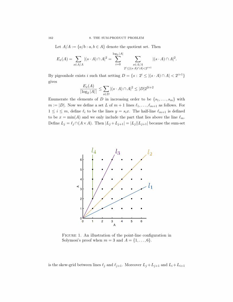
162 8. THE SUM-PRODUCT PROBLEM
Let A/A := a/b : a, b ∈ A denote the quotient set. Then
Ex(A) =∑s∈A/A
|(s ·A) ∩A|2 =
log2 |A|∑i=0
∑s∈A/A
2i≤|(s·A)∩A|<2i+1
|(s ·A) ∩A|2.
By pigeonhole exists i such that setting D = s : 2i ≤ |(s · A) ∩ A| < 2i+1gives
Ex(A)
dlog2 |A|e≤∑s∈D|(s ·A) ∩A|2 ≤ |D|22i+2
Enumerate the elements of D in increasing order to be s1, . . . , sm withm := |D|. Now we define a set L of m+ 1 lines `1, . . . , `m+1 as follows. For1 ≤ i ≤ m, define `i to be the lines y = six. The half-line `m+1 is definedto be x = min(A) and we only include the part that lies above the line `m.Define Lj = `j ∩(A×A). Then |Lj +Lj+1| = |Lj ||Lj+1| because the sum-set
Figure 1. An illustration of the point-line configuration inSolymosi’s proof when m = 3 and A = 1, . . . , 6.
is the skew-grid between lines `j and `j+1. Moreover Lj+Lj+1 and Li+Li+1
8. SZEMERÉDI-TROTTER AND INCIDENCE GEOMETRY 163
are disjoint if i 6= j. Thus
|A+A|2 = |(A×A) + (A×A)|
≥m∑j=1
|Lj + Lj+1|
=m∑j=1
|Lj ||Lj+1| ≥ m22i
But above we showed that Ex(A)dlog2 |A|e ≤ m22i+2. Combining the last two
equations implies Equationeqn:solyeqn:soly10 and the proof of Solymosi’s result.
Remark 8.14. One can slightly improve the exponent by analyzing what hap-pens between two lines that are non-consecutive in Solymosi’s proof.
It is natural to investigate the sum-product problem over the finite fields.
Theorem 8.15 (Bourgain-Katz-Tao [7]). For all δ > 0, there exists c > 0
such that if p is prime, A ⊂ Fp, and |A| ≤ p1−δ, then
max|A+A|, |AA| ≥ |A|1+c.
One can interpret this theorem as saying that Fp does not have anyapproximate sub-rings, for in any bona-fide subring A, we know that A+A =
AA = A.


References
Oei17 1. The on-line encyclopedia of integer sequences, https://oeis.org/A186705, Accessed:2017-09-19.
ACNS82 2. Miklós Ajtai, Vašek Chvátal, Monroe M Newborn, and Endre Szemerédi, Crossing-freesubgraphs, North-Holland Mathematics Studies 60 (1982), 9–12.
ARS99 3. Noga Alon, Lajos Rónyai, and Tibor Szabó, Norm-graphs: variations and applications,Journal of Combinatorial Theory, Series B 76 (1999), no. 2, 280–290.
BHP01 4. Roger C Baker, Glyn Harman, and János Pintz, The difference between consecutiveprimes, ii, Proceedings of the London Mathematical Society 83 (2001), no. 3, 532–562.
BL96 5. V. Bergelson and A. Leibman, Polynomial extensions of van der Waerden’s and Sze-merédi’s theorems, J. Amer. Math. Soc. 9 (1996), no. 3, 725–753. MR 1325795(96j:11013)
BBK13 6. Pavle VM Blagojević, Boris Bukh, and Roman Karasev, Turán numbers for ks, t-freegraphs: topological obstructions and algebraic constructions, Israel Journal of Mathe-matics 197 (2013), no. 1, 199–214.
BKT04 7. J. Bourgain, N. Katz, and T. Tao, A sum-product estimate in finite fields, and appli-cations, Geometric and Functional Analysis 14 (2004), no. 1, 27–57.
Bro66 8. William G Brown, On graphs that do not contain a thomsen graph, Canad. Math. Bull9 (1966), no. 2, 1–2.
Buk15 9. Boris Bukh, Random algebraic construction of extremal graphs, Bulletin of the LondonMathematical Society 47 (2015), no. 6, 939–945.
Dav13 10. Harold Davenport, Multiplicative number theory, vol. 74, Springer Science & BusinessMedia, 2013.
Dic52 11. LE Dickson, History of the theory of numbers, ii. chelsea, New York (1952).durrett2010probability 12. Rick Durrett, Probability: theory and examples, Cambridge university press, 2010.
Ele97 13. G. Elekes, On the number of sums and products, Acta Arithmetica LXXX1.4 (1997),365–367.
Erd46 14. p. Erdős, On the number of sums and products, American Mathematical Monthly 53(1946), 248–250.
ET36 15. P. Erdős and Paul Turán, On Some Sequences of Integers, J. London Math. Soc. 11(1936), 261–264. MR 1574918
ERS66 16. Paul Erdős, A Rényi, and VT Sós, On a problem of graph theory, Studia Sci. Math.Hungar 1 (1966), no. 215, C235.
FS11DRC 17. Jacob Fox and Benny Sudakov, Dependent random choice, Random Structures Algo-rithms 38 (2011), no. 1-2, 68–99. MR 2768884
165

166 REFERENCES
Fur77 18. H. Furstenberg, Ergodic behavior of diagonal measures and a theorem of Szemerédion arithmetic progressions, J. Analyse Math. 31 (1977), 204–256. MR 0498471 (58#16583)
Fur81 19. , Recurrence in ergodic theory and combinatorial number theory, PrincetonUniversity Press, Princeton, N.J., 1981, M. B. Porter Lectures. MR 603625
FK78 20. H. Furstenberg and Y. Katznelson, An ergodic Szemerédi theorem for commutingtransformations, J. Analyse Math. 34 (1978), 275–291. MR 531279 (82c:28032)
FKO82 21. H. Furstenberg, Y. Katznelson, and D. Ornstein, The ergodic theoretical proof of Sze-merédi’s theorem, Bull. Amer. Math. Soc. 7 (1982), no. 3, 527–552. MR 670131(84b:28016)
Gow01 22. W. T. Gowers, A new proof of Szemerédi’s theorem, Geom. Funct. Anal. 11 (2001),no. 3, 465–588. MR 1844079 (2002k:11014)
Gow07 23. , Hypergraph regularity and the multidimensional Szemerédi theorem, Ann. ofMath. 166 (2007), no. 3, 897–946. MR 2373376 (2009d:05250)
GT08 24. B. Green and T. Tao, The primes contain arbitrarily long arithmetic progressions,Ann. of Math. 167 (2008), no. 2, 481–547.
GK10 25. Larry Guth and Nets Hawk Katz, On the erdos distinct distance problem in the plane,arXiv preprint arXiv:1011.4105 (2010).
HW79 26. Godfrey Harold Hardy and Edward Maitland Wright, An introduction to the theoryof numbers, Oxford University Press, 1979.
Hoh30 27. G. Hoheisel, Primzahlprobleme in der Analysis., Sitzungsber. Preuß. Akad. Wiss.,Phys.-Math. Kl. 1930 (1930), 580–588 (German).
KRS96 28. János Kollár, Lajos Rónyai, and Tibor Szabó, Norm-graphs and bipartite turán num-bers, Combinatorica 16 (1996), no. 3, 399–406.
Lei83 29. Frank Thomson Leighton, Complexity issues in vlsi: optimal layouts for the shuffle-exchange graph and other networks, MIT press, 1983.
mesh95 30. Roy Meshulam, On subsets of finite abelian groups with no 3-term arithmetic progres-sions, J. Comb. Theory, Ser. A 71 (1995), no. 1, 168–172.
MV06 31. Hugh L Montgomery and Robert C Vaughan, Multiplicative number theory i: Classicaltheory, vol. 97, Cambridge University Press, 2006.
NRS06 32. B. Nagle, V. Rödl, and M. Schacht, The counting lemma for regular k-uniform hy-pergraphs, Random Structures Algorithms 28 (2006), no. 2, 113–179. MR 2198495(2007d:05084)
Pre17 33. S. Prendiville, Quantitative bounds in the polynomial Szemerédi theorem: the homo-geneous case, Discrete Anal. (2017), Paper No. 5, 34. MR 3631611
Ram30 34. F. P. Ramsey, On a problem of formal logic, Proc. London Math. Soc. Ser. 2 30 (1930),264–286.
RNSSK05 35. V. Rödl, B. Nagle, J. Skokan, M. Schacht, and Y. Kohayakawa, The hypergraph reg-ularity method and its applications, Proc. Natl. Acad. Sci. USA 102 (2005), no. 23,8109–8113. MR 2167756
RS07b 36. V. Rödl and M. Schacht, Regular partitions of hypergraphs: counting lemmas, Combin.Probab. Comput. 16 (2007), no. 6, 887–901. MR 2351689 (2008j:05238)
RS07a 37. , Regular partitions of hypergraphs: regularity lemmas, Combin. Probab. Com-put. 16 (2007), no. 6, 833–885. MR 2351688 (2008h:05083)

REFERENCES 167
RS04 38. V. Rödl and J. Skokan, Regularity lemma for k-uniform hypergraphs, Random Struc-tures Algorithms 25 (2004), no. 1, 1–42.
RS06 39. , Applications of the regularity lemma for uniform hypergraphs, Random Struc-tures Algorithms 28 (2006), no. 2, 180–194.
Roth53 40. K. F. Roth, On certain sets of integers, J. London Math. Soc. 28 (1953), 104–109.MR 0051853 (14,536g)
RS78 41. I. Z. Ruzsa and E. Szemerédi, Triple systems with no six points carrying three trian-gles, Combinatorics (Proc. Fifth Hungarian Colloq., Keszthely, 1976), Vol. II, Colloq.Math. Soc. János Bolyai, vol. 18, North-Holland, Amsterdam, 1978, pp. 939–945.MR 519318 (80c:05116)
Sar78 42. A. Sárkőzy, On difference sets of sequences of integers. I, Acta Math. Acad. Sci.Hungar. 31 (1978), no. 1–2, 125–149. MR 0466059 (57 #5942)
Sch93 43. C Schade, Exakte maximalzahlen gleicher abst ande, Ph.D. thesis, Diplomarbeit beiH. Harborth, Universit at Braunschweig, 1993.
Sch16 44. I. Schur, Über die Kongruenz xm + ym = zm (mod. p), Jahresber. Deutsche Math.-Verein. 25 (1916), 114–116.
Sha48 45. Claude E Shannon, A mathematical theory of communication, part i, part ii, Bell Syst.Tech. J. 27 (1948), 623–656.
Sol05 46. J. Solymosi, On the number of sums and products, Bulletin of the London Mathemat-ical Society 37 (2005), 491–494.
Sop10 47. Ivan Soprounov, A short proof of the prime number theorem for arithmetic progres-sions, preprint (2010).
SST84 48. Joel Spencer, Endre Szemerédi, and William T Trotter, Unit distances in the euclideanplane, Graph theory and combinatorics (1984), 293–303.
Sze97 49. László A Székely, Crossing numbers and hard erdős problems in discrete geometry,Combinatorics, Probability and Computing 6 (1997), no. 3, 353–358.
Sze69 50. E. Szemerédi, On sets of integers containing no four elements in arithmetic progres-sion, Acta Math. Acad. Sci. Hungar. 20 (1969), 89–104. MR 0245555
Sze75 51. , On sets of integers containing no k elements in arithmetic progression, ActaArith. 27 (1975), 199–245.
Sze78 52. , Regular partitions of graphs, Problèmes combinatoires et théorie des graphes(Colloq. Internat. CNRS, Univ. Orsay, Orsay, 1976), Colloq. Internat. CNRS, vol. 260,CNRS, Paris, 1978, pp. 399–401. MR 540024 (81i:05095)
Sze16 53. Endre Szemerédi, Erdős’s unit distance problem, pp. 459–477, Springer InternationalPublishing, Cham, 2016.
vdW27 54. B.L. van der Waerden, Beweis einer Baudetschen Vermutung, Nieuw Arch. Wisk. 15(1927), 212—216.