graph based convolutional neural network - bmva · 2017-05-30 · edwards, xie: graph convolutional...

EDWARDS, XIE: GRAPH CONVOLUTIONAL NEURAL NETWORK 1

Graph Based Convolutional Neural NetworkMichael Edwards

Xianghua Xiehttp://www.csvision.swan.ac.uk

Swansea UniversitySwansea, UK

Abstract

The benefit of localized features within the regular domain has given rise to the useof Convolutional Neural Networks (CNNs) in machine learning, with great proficiencyin the image classification. The use of CNNs becomes problematic within the irregularspatial domain due to design and convolution of a kernel filter being non-trivial. One so-lution to this problem is to utilize graph signal processing techniques and the convolutiontheorem to perform convolutions on the graph of the irregular domain to obtain featuremap responses to learnt filters. We propose graph convolution and pooling operatorsanalogous to those in the regular domain. We also provide gradient calculations on theinput data and spectral filters, which allow for the deep learning of an irregular spatial do-main problem. Signal filters take the form of spectral multipliers, applying convolutionin the graph spectral domain. Applying smooth multipliers results in localized convo-lutions in the spatial domain, with smoother multipliers providing sharper feature maps.Algebraic Multigrid is presented as a graph pooling method, reducing the resolution ofthe graph through agglomeration of nodes between layers of the network. Evaluation ofperformance on the MNIST digit classification problem in both the regular and irregu-lar domain is presented, with comparison drawn to standard CNN. The proposed graphCNN provides a deep learning method for the irregular domains present in the machinelearning community, obtaining 94.23% on the regular grid, and 94.96% on a spatiallyirregular subsampled MNIST.

1 IntroductionIn recent years, the machine learning and pattern recognition community has seen a resur-gence in the use of neural network and deep learning architecture for the understanding ofclassification problems. Standard fully connected neural networks have been utilized fordomain problems within the feature space with great effect, from text document analysis togenome characterization [22]. The introduction of the CNN provided a method for iden-tifying locally aggregated features by utilizing kernel filter convolutions across the spatialdimensions of the input to extract feature maps [10]. Applications of CNNs have shownstrong levels of recognition in problems from face detection [11], digit classification [4], andclassification on a large number of classes [15].

The core CNN concept introduces the hidden convolution and pooling layers to identifyspatially localized features via a set of receptive fields in kernel form. The convolutionoperator takes an input and convolves kernel filters across the spatial domain of the data

c© 2016. The copyright of this document resides with its authors.It may be distributed unchanged freely in print or electronic forms.

Pages 114.1-114.11

DOI: https://dx.doi.org/10.5244/C.30.114

https://dx.doi.org/10.5244/C.30.114

2 EDWARDS, XIE: GRAPH CONVOLUTIONAL NEURAL NETWORK

provided some stride and padding parameters, returning feature maps that represent responseto the filters. Given a multi-channel input, a feature map is the summation of the convolutionswith separate kernels for each input channel. In CNN architecture, the pooling operator isutilized to compress the resolution of each feature map in the spatial dimensions, leavingthe number of feature maps unchanged. Applying a pooling operator across a feature mapenables the algorithm to handle a growing number of feature maps and generalizes the featuremaps by resolution reduction. Common pooling operations are that of taking the average andmax of receptive cells over the input map [1].

Due to the usage of convolutions for the extraction of partitioning features, CNNs re-quire an assumption that the topology of the input dimensions provides some spatially reg-ular sense of locality. Convolution on the regular grid is well documented and present ina variety of CNN implementations [9, 20], however when moving to domains that are notsupported by the regular low-dimensional grid, convolution becomes an issue. Many ap-plication domains utilize irregular feature spaces [13], and in such domains it may not bepossible to define a spatial kernel filter or identify a method of translating such a kernelacross spatial domain. Methods of handling such an irregular space as an input include usingstandard neural networks, embedding the feature space onto a grid to allow convolution [8],identifying local patches on the irregular manifold to perform geodesic convolutions [14],or graph signal processing based convolutions on graph signal data [7]. The potential appli-cations of a convolutional network in the spatially irregular domain are expansive, howeverthe graph convolution and pooling is not trivial, with graph representations of data being thetopic of ongoing research [5, 21]. The use of graph representation of data for deep learningis introduced by [3], utilizing the Laplacian spectrum for feature mining from the irregulardomain. This is further expanded upon in [7], providing derivative calculations for the back-propagation of errors during gradient descent. We formulate novel gradient equations thatshow more stable calculations in relation to both the input data and the tracked weights inthe network.

In this methodology-focused study, we explore the use of graph based signal-processingtechniques for convolutional networks on irregular domain problems. We evaluate two meth-ods of graph pooling operators and report the effects of using interpolation in the spectraldomain for identifying localized filters. We evaluate the use of Algebraic Multigrid agglom-eration for graph pooling. We have also identified an alternative to the gradient calculationsof [7] by formulating the gradients in regards to the input data as the spectral convolution ofthe gradients of the output with the filters (Equation 2), and the gradients for the weights asthe spectral convolution of the input and output gradients (Equation 3). These proposed gra-dient calculations show consistent stability over previous methods [7], which in turn benefitsthe gradient based training of the network. Results are reported on the MNIST dataset andthe subsampled MNIST on an irregular grid.

The rest of the paper is outlined as follows. Section 2 describes the generation of a graphbased CNN architecture, providing the convolution and pooling layers in the graph domainby use of signal-processing on the graph. Section 3 details the experimental evaluation ofthe proposed methods and a comparison against the current state of the art, with Section 4reporting the results found and conclusions drawn in Section 5.


Output Predic,on

Fully Connected Network

Graph Formula,on

Graph Convolu,onal Neural Network Operators

Pooling Layers

Convolu,on Layers

O Feature Maps Graph Signal Spectral Form

O Smooth Spectral Mul,pliers 0 10 20 30 40 50 60 70 80 90 100

-25

-20

-15

-10

-5

0

5

10

15

20

25

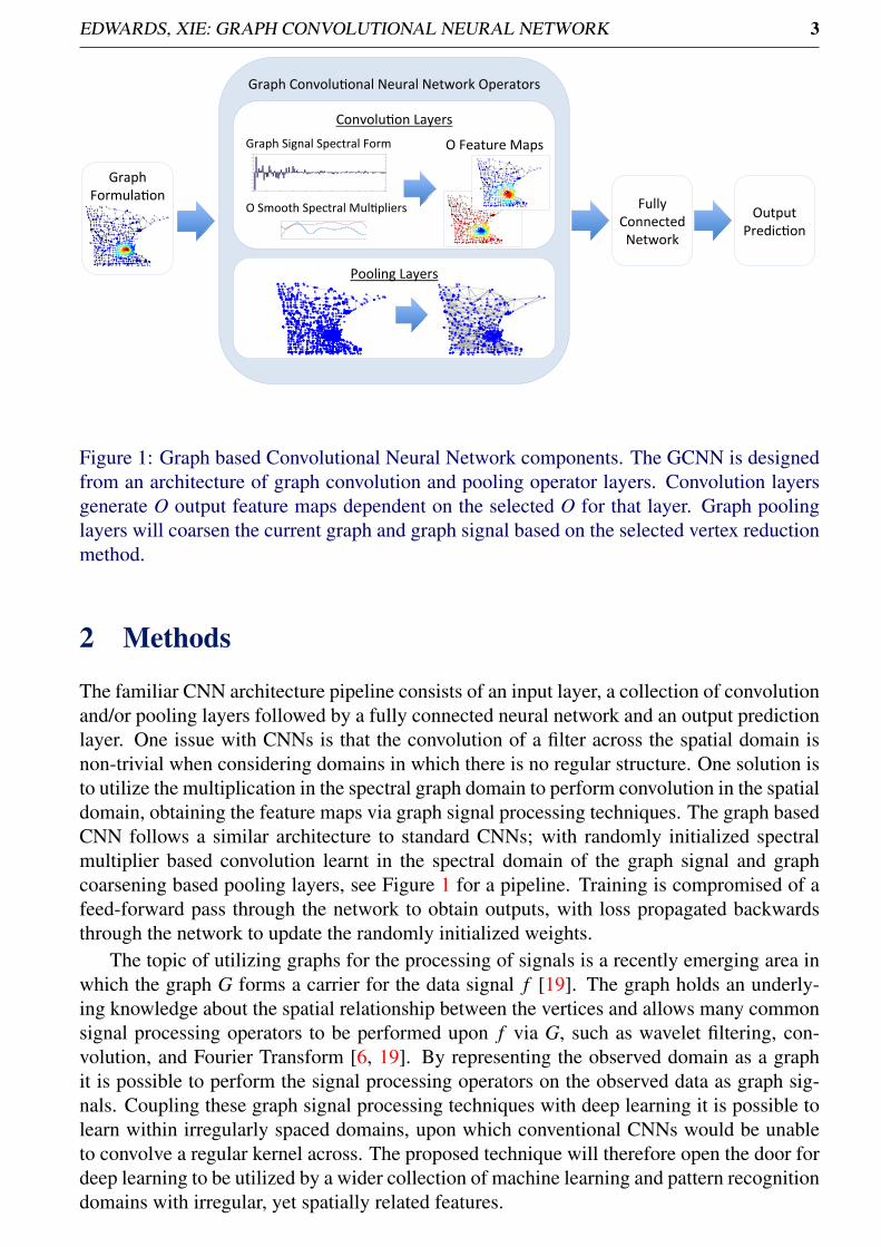
Figure 1: Graph based Convolutional Neural Network components. The GCNN is designedfrom an architecture of graph convolution and pooling operator layers. Convolution layersgenerate O output feature maps dependent on the selected O for that layer. Graph poolinglayers will coarsen the current graph and graph signal based on the selected vertex reductionmethod.

2 Methods

The familiar CNN architecture pipeline consists of an input layer, a collection of convolutionand/or pooling layers followed by a fully connected neural network and an output predictionlayer. One issue with CNNs is that the convolution of a filter across the spatial domain isnon-trivial when considering domains in which there is no regular structure. One solution isto utilize the multiplication in the spectral graph domain to perform convolution in the spatialdomain, obtaining the feature maps via graph signal processing techniques. The graph basedCNN follows a similar architecture to standard CNNs; with randomly initialized spectralmultiplier based convolution learnt in the spectral domain of the graph signal and graphcoarsening based pooling layers, see Figure 1 for a pipeline. Training is compromised of afeed-forward pass through the network to obtain outputs, with loss propagated backwardsthrough the network to update the randomly initialized weights.

The topic of utilizing graphs for the processing of signals is a recently emerging area inwhich the graph G forms a carrier for the data signal f [19]. The graph holds an underly-ing knowledge about the spatial relationship between the vertices and allows many commonsignal processing operators to be performed upon f via G, such as wavelet filtering, con-volution, and Fourier Transform [6, 19]. By representing the observed domain as a graphit is possible to perform the signal processing operators on the observed data as graph sig-nals. Coupling these graph signal processing techniques with deep learning it is possible tolearn within irregularly spaced domains, upon which conventional CNNs would be unableto convolve a regular kernel across. The proposed technique will therefore open the door fordeep learning to be utilized by a wider collection of machine learning and pattern recognitiondomains with irregular, yet spatially related features.


Figure 2: Eigenvectors ui={2,20,40} of the full 28×28 regular gird (left) and the subsampledirregular grid (right).

2.1 Convolution on GraphA graph G = {V,W} consists of N vertices V and the weights W of the undirected, non-negative, non-selflooping edges between two vertices vi and v j. The unnormalized graphLaplacian matrix L is defined as L = D−W , where di,i = ∑N

i=1 ai forms a diagonal matrixcontaining the sum of all adjacencies for a vertex. Given G, an observed data sample is asignal f ∈ RN that resides on G, where fi corresponds to the signal amplitude at vertex vi.

Convolution is one of the two key operations in the CNN architecture, allowing for lo-cally receptive features to be highlighted in the input image [10]. A similar operator ispresented in graph based CNN, however due to the potentially irregular domain graph con-volution makes use of the convolution theorem of convolution in the spatial domain being amultiplication in the frequency domain [2].To project the graph signal into the frequency domain, the Laplacian L is decomposed into afull matrix of orthonormal eigenvectors U = {ui=1...N}, where ui is a column of the matrix U ,and the vector of associated eigenvalues λi=1...N [19], Figure 2. The forward Graph FourierTransform is therefore given for a given signal as fi = ∑N

l=1 λl f Ti ui, and its corresponding

inverse fi = ∑Nl=1 λl fiui. Using the matrix U the Fourier transform is defined as f = UT f ,

and the inverse as f =U f , where UT is the transpose of the eigenvector matrix.For forward convolution, a convolutional operator in the vertex domain can be composed

as a multiplication in the Fourier space of the Laplacian operator [2]. Given the spectralform of our graph signal f ∈ RN and the spectral multiplier k ∈ RN , the convolved outputsignal in the original spatial domain is the spectral multipication, i.e. y =U f k. It is possibleto expand this for multiple input channels and multiple output feature maps:

ys,o =UI

∑i=1

UT fs,i� ki,o , (1)

where I is the number of input channels for f , s is a given batch sample, and o indexes anoutput feature map from O output maps.

Localized regions in the spatial domain are defined by the kernel receptive field in CNNs,and for graph based CNNs the spatial vertex domain localization is given by a smoothnesswithin the spectral domain. Therefore to identify local features within the spatial domain thespectral multipliers used for spectral convolution are identified by tracking a subsampled setof filter weights ki,ok ∈ R<N which are interpolated up to a full filter via a smoothing kernelΦ such as cubic splines: ki,o = Φki,o. This has the added benefit of reducing the number oftracked weights, however leads to an extra pair of operations in interpolating the weights tothe full k ∈ RN for multiplication. Reducing the number of tracked weights increases thesmoothness of the final interpolated filter, and lowering the tuning parameter of the numberof tracked weights learns sharper features.


2.2 Backpropagation on Graph

Backpropagation of errors is a pivotal component of deep learning, providing updates ofweights and bias for the networks towards the target function with gradient descent. Thisrequires obtaining derivatives in regards to the input and weights used to generate the output,in the case of graph based CNN convolution the gradients are formulated in regards to thegraph signal f and the spectral multipliers k. The gradients for an input feature map channelfs,i is given as the convolution of the gradients for the output ∇y and the spectral multipliersin the spectral domain via

∇ fs,i =UO

∑o=1

UT ∇ys,o� ki,o (2)

for a provided batch of S graph signals. Gradients for the full set of interpolated spectralmultipliers is formulated as the convolution of the gradients for the output ∇y with the inputfs,i via

∇ki,o =N

∑s=1

UT ∇ys,o�UT fs,i. (3)

As the filters are spectral domain multipliers, we do not project this spectral convolutionback through the graph Fourier transform. The smooth multiplier weights ∇k can then beprojected back to the subsampled set of tracked weights by the multiplication with the in-versed smoothing kernel ∇ki,o = ΦT ∇ki,o.

2.3 Pooling on Graph

The pooling layer is the second component in conventional CNN, reducing the resolution ofthe input feature map in both an attempt to generalize the features identified and to managethe memory complexity when using numerous filters [1]. During graph based convolutionsthere is no reduction in size between the input signal and the output feature map due tothe multiplication of the RN filter with the RN spectral signal. As such, each layer of adeep graph CNN would possess a graph with RN vertices. Such a construction could bebeneficial, as this would allow the algorithm to store a single instance of the graph and theassociated N2 eigenvector matrix U . If pooling is utilized, there is benefit gained from thefeature map generalization and the reduction in complexity of the graph Fourier transformsas each layer’s vertex count N is lowered. To pool local features together on the graph, it isrequired to perform graph coarsening and project the input feature maps through to the new,reduced size graph. Coarsening G = {V,W} to G = {V ,W} not only requires the reductionof vertex counts, but also a handling of edges between the remaining N vertices. Commonmethods of generating V are to either select a subset of V to carry forward to G [18] or toform completely new set of nodes V from some aggregation of related nodes within V [16].One method for selection of V can be achieved by selecting the largest eigenvalue λN andsplitting V into two subsets based on the polarity of the associated eigenvector UN [12]. Wecan therefore define V = {uN , i};uN , i >= 0 and its complement V c = {uN , i};uN , i < 0. V isthen utilized to construct the graph G, although by reversing the selection for the polarity tokeep it is just as understandable to choose V c for construction of G.

In this study we utilize Algebraic Multigrid (AMG) for graph coarsening, a method ofprojecting signals to a coarser graph representation obtained via greedy selection of vertices[16]. Aggregation takes a subset of vertices on V and generates a singular vertex in the new


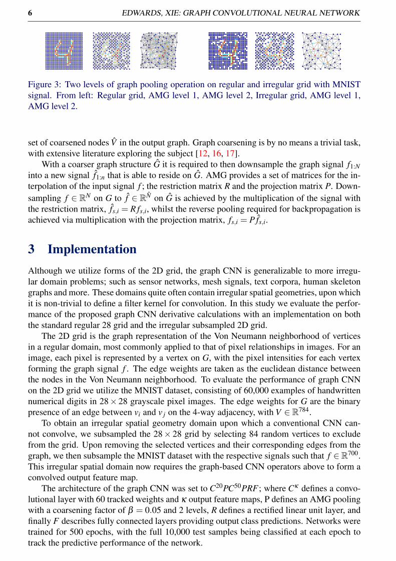
Figure 3: Two levels of graph pooling operation on regular and irregular grid with MNISTsignal. From left: Regular grid, AMG level 1, AMG level 2, Irregular grid, AMG level 1,AMG level 2.

set of coarsened nodes V in the output graph. Graph coarsening is by no means a trivial task,with extensive literature exploring the subject [12, 16, 17].

With a coarser graph structure G it is required to then downsample the graph signal f1:Ninto a new signal f1:n that is able to reside on G. AMG provides a set of matrices for the in-terpolation of the input signal f ; the restriction matrix R and the projection matrix P. Down-sampling f ∈ RN on G to f ∈ RN on G is achieved by the multiplication of the signal withthe restriction matrix, fs,i = R fs,i, whilst the reverse pooling required for backpropagation isachieved via multiplication with the projection matrix, fs,i = P fs,i.

3 ImplementationAlthough we utilize forms of the 2D grid, the graph CNN is generalizable to more irregu-lar domain problems; such as sensor networks, mesh signals, text corpora, human skeletongraphs and more. These domains quite often contain irregular spatial geometries, upon whichit is non-trivial to define a filter kernel for convolution. In this study we evaluate the perfor-mance of the proposed graph CNN derivative calculations with an implementation on boththe standard regular 28 grid and the irregular subsampled 2D grid.

The 2D grid is the graph representation of the Von Neumann neighborhood of verticesin a regular domain, most commonly applied to that of pixel relationships in images. For animage, each pixel is represented by a vertex on G, with the pixel intensities for each vertexforming the graph signal f . The edge weights are taken as the euclidean distance betweenthe nodes in the Von Neumann neighborhood. To evaluate the performance of graph CNNon the 2D grid we utilize the MNIST dataset, consisting of 60,000 examples of handwrittennumerical digits in 28× 28 grayscale pixel images. The edge weights for G are the binarypresence of an edge between vi and v j on the 4-way adjacency, with V ∈ R784.

To obtain an irregular spatial geometry domain upon which a conventional CNN can-not convolve, we subsampled the 28× 28 grid by selecting 84 random vertices to excludefrom the grid. Upon removing the selected vertices and their corresponding edges from thegraph, we then subsample the MNIST dataset with the respective signals such that f ∈R700.This irregular spatial domain now requires the graph-based CNN operators above to form aconvolved output feature map.

The architecture of the graph CNN was set to C20PC50PRF ; where Cκ defines a convo-lutional layer with 60 tracked weights and κ output feature maps, P defines an AMG poolingwith a coarsening factor of β = 0.05 and 2 levels, R defines a rectified linear unit layer, andfinally F describes fully connected layers providing output class predictions. Networks weretrained for 500 epochs, with the full 10,000 test samples being classified at each epoch totrack the predictive performance of the network.


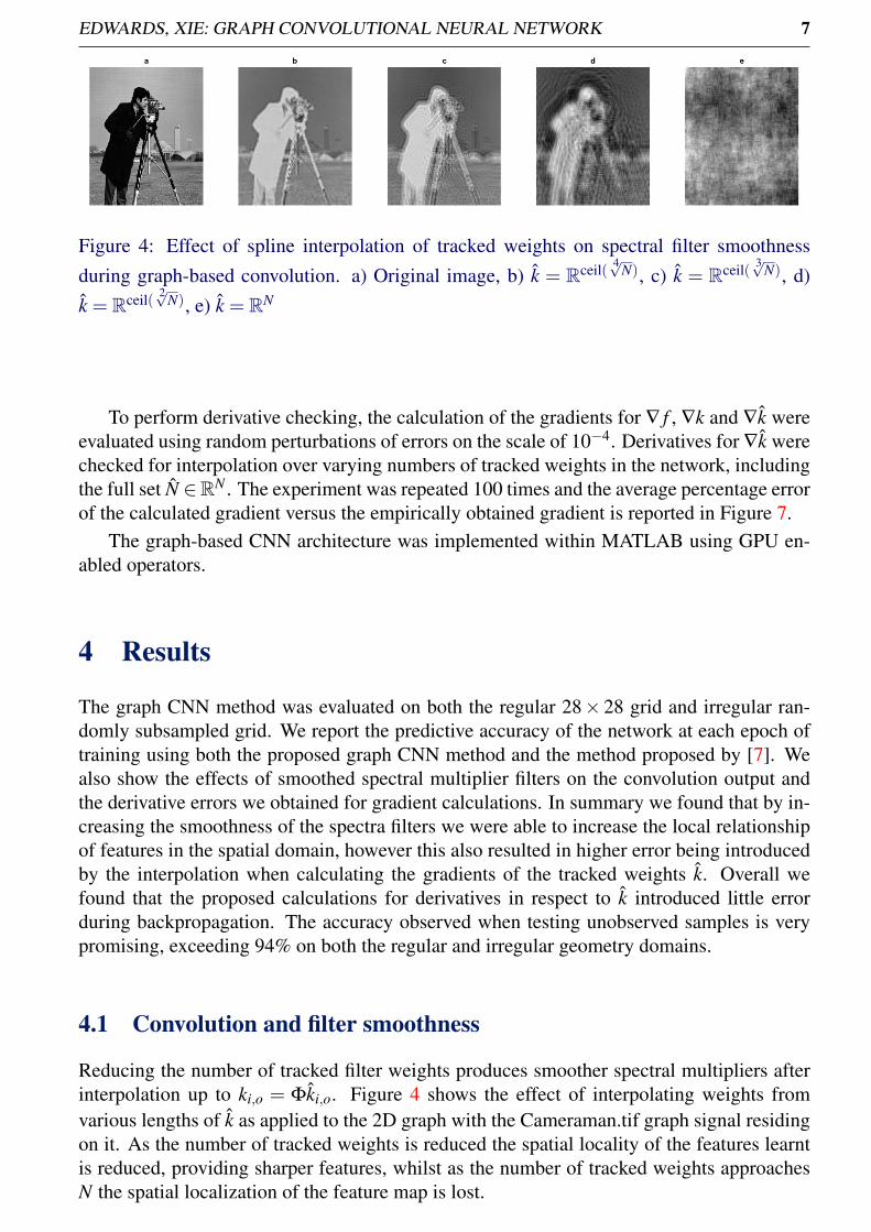
Figure 4: Effect of spline interpolation of tracked weights on spectral filter smoothnessduring graph-based convolution. a) Original image, b) k = Rceil( 4√N), c) k = Rceil( 3√N), d)k = Rceil( 2√N), e) k = RN

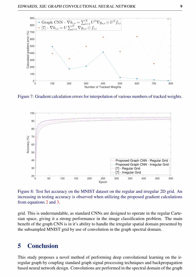
To perform derivative checking, the calculation of the gradients for ∇ f , ∇k and ∇k wereevaluated using random perturbations of errors on the scale of 10−4. Derivatives for ∇k werechecked for interpolation over varying numbers of tracked weights in the network, includingthe full set N ∈RN . The experiment was repeated 100 times and the average percentage errorof the calculated gradient versus the empirically obtained gradient is reported in Figure 7.

The graph-based CNN architecture was implemented within MATLAB using GPU en-abled operators.

4 Results

The graph CNN method was evaluated on both the regular 28× 28 grid and irregular ran-domly subsampled grid. We report the predictive accuracy of the network at each epoch oftraining using both the proposed graph CNN method and the method proposed by [7]. Wealso show the effects of smoothed spectral multiplier filters on the convolution output andthe derivative errors we obtained for gradient calculations. In summary we found that by in-creasing the smoothness of the spectra filters we were able to increase the local relationshipof features in the spatial domain, however this also resulted in higher error being introducedby the interpolation when calculating the gradients of the tracked weights k. Overall wefound that the proposed calculations for derivatives in respect to k introduced little errorduring backpropagation. The accuracy observed when testing unobserved samples is verypromising, exceeding 94% on both the regular and irregular geometry domains.

4.1 Convolution and filter smoothness

Reducing the number of tracked filter weights produces smoother spectral multipliers afterinterpolation up to ki,o = Φki,o. Figure 4 shows the effect of interpolating weights fromvarious lengths of k as applied to the 2D graph with the Cameraman.tif graph signal residingon it. As the number of tracked weights is reduced the spatial locality of the features learntis reduced, providing sharper features, whilst as the number of tracked weights approachesN the spatial localization of the feature map is lost.


Figure 5: Feature maps formed by a feed-forward pass of the regular domain. From left:Original image, Convolution round 1, Pooling round 1, Convolution round 2, Pooling round2.

Figure 6: Feature maps formed by a feed-forward pass of the irregular domain. From left:Original image, Convolution round 1, Pooling round 1, Convolution round 2, Pooling round2.

4.2 Localized feature mapsBy interpolating smooth spectral multipliers from the 60 tracked weights we were able toconvolve over the irregular domain to produce feature maps in the spatial domain with spa-tially localized features. Figure 6 visualizes output for each layer of the Graph CNN convo-lution and pooling layers for both the regular and irregular domain graphs.

4.3 Backpropagation derivative checksThe proposed method gave an average of 1.41%(±4.00%) error in the calculation of the gra-dients for the input feature map. In comparison, by not first applying a graph Fourier trans-form to ∇ys,o in the calculation for ∇ fs,i, as in [7], we obtain errors of 376.50%(±1020.79%).Similarly the proposed method of obtaining the spectral forms of ∇ys,o and fs,i in the calcu-lation of ∇ki,o gave errors of 3.81%(±16.11%). By not projecting to the spectral forms ofthese inputs, errors of 826.08%(±4153.32%) are obtained. Figure 7 shows the average per-centage derivative calculation error for ∇k of varying numbers of tracked weights over 100runs. The proposed method of gradient calculation shows lower errors than the comparedmethod gradient calculation of ∇k when k ∈ RN and all but the lowest number of trackedweights of k ∈R100. The introduction of interpolation leads to a higher introduction of errorinto the calculated gradient errors, especially in the presence of a low number of trackedweights.

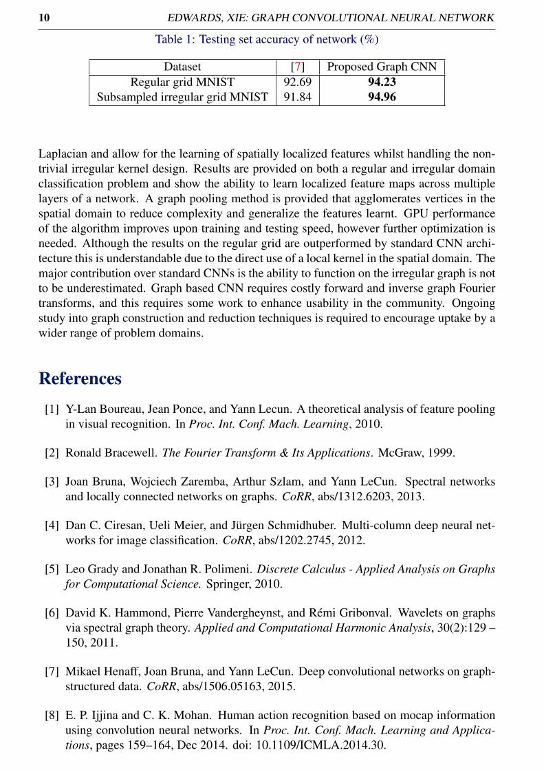
4.4 Testing performanceClassification performance on the MNIST dataset is reported in Table 1, with progressionof testing accuracy over epochs given in Figure 8 comparing between the proposed gradientcalculations and those of [7]. The proposed graph CNN method does not obtain the 99.77%accuracy rates of the state of the art CNN architecture presented by [4] on the full 28×28


0 100 200 300 400 500 600 700 800

Number of Tracked Weights

0

100

200

300

400

500

600

700

800

900

Calc

ula

ted g

radie

nt err

or

(%)

Graph CNN - ∇ki,o =∑N

s=1 UT∇ys,o ⊙ UT fs,i

[7] - ∇ki,o = U∑N

s=1 ∇ys,o ⊙ fs,i

Figure 7: Gradient calculation errors for interpolation of various numbers of tracked weights.

0 50 100 150 200 250 300 350 400 450 500

Epoch

20

30

40

50

60

70

80

90

100

Accura

cy (

%)

Proposed Graph CNN - Regular Grid

Proposed Graph CNN - Irregular Grid

[7] - Regular Grid

[7] - Irregular Grid

Figure 8: Test Set accuracy on the MNIST dataset on the regular and irregular 2D grid. Anincreasing in testing accuracy is observed when utilizing the proposed gradient calculationsfrom equations 2 and 3.

grid. This is understandable, as standard CNNs are designed to operate in the regular Carte-sian space, giving it a strong performance in the image classification problem. The mainbenefit of the graph CNN is in it’s ability to handle the irregular spatial domain presented bythe subsampled MNIST grid by use of convolution in the graph spectral domain.

5 Conclusion

This study proposes a novel method of performing deep convolutional learning on the ir-regular graph by coupling standard graph signal processing techniques and backpropagationbased neural network design. Convolutions are performed in the spectral domain of the graph


Table 1: Testing set accuracy of network (%)

Dataset [7] Proposed Graph CNNRegular grid MNIST 92.69 94.23

Subsampled irregular grid MNIST 91.84 94.96

Laplacian and allow for the learning of spatially localized features whilst handling the non-trivial irregular kernel design. Results are provided on both a regular and irregular domainclassification problem and show the ability to learn localized feature maps across multiplelayers of a network. A graph pooling method is provided that agglomerates vertices in thespatial domain to reduce complexity and generalize the features learnt. GPU performanceof the algorithm improves upon training and testing speed, however further optimization isneeded. Although the results on the regular grid are outperformed by standard CNN archi-tecture this is understandable due to the direct use of a local kernel in the spatial domain. Themajor contribution over standard CNNs is the ability to function on the irregular graph is notto be underestimated. Graph based CNN requires costly forward and inverse graph Fouriertransforms, and this requires some work to enhance usability in the community. Ongoingstudy into graph construction and reduction techniques is required to encourage uptake by awider range of problem domains.

References[1] Y-Lan Boureau, Jean Ponce, and Yann Lecun. A theoretical analysis of feature pooling

in visual recognition. In Proc. Int. Conf. Mach. Learning, 2010.

[2] Ronald Bracewell. The Fourier Transform & Its Applications. McGraw, 1999.

[3] Joan Bruna, Wojciech Zaremba, Arthur Szlam, and Yann LeCun. Spectral networksand locally connected networks on graphs. CoRR, abs/1312.6203, 2013.

[4] Dan C. Ciresan, Ueli Meier, and Jürgen Schmidhuber. Multi-column deep neural net-works for image classification. CoRR, abs/1202.2745, 2012.

[5] Leo Grady and Jonathan R. Polimeni. Discrete Calculus - Applied Analysis on Graphsfor Computational Science. Springer, 2010.

[6] David K. Hammond, Pierre Vandergheynst, and Rémi Gribonval. Wavelets on graphsvia spectral graph theory. Applied and Computational Harmonic Analysis, 30(2):129 –150, 2011.

[7] Mikael Henaff, Joan Bruna, and Yann LeCun. Deep convolutional networks on graph-structured data. CoRR, abs/1506.05163, 2015.

[8] E. P. Ijjina and C. K. Mohan. Human action recognition based on mocap informationusing convolution neural networks. In Proc. Int. Conf. Mach. Learning and Applica-tions, pages 159–164, Dec 2014. doi: 10.1109/ICMLA.2014.30.


[9] Yangqing Jia, Evan Shelhamer, Jeff Donahue, Sergey Karayev, Jonathan Long, RossGirshick, Sergio Guadarrama, and Trevor Darrell. Caffe: Convolutional architecturefor fast feature embedding. arXiv:1408.5093, 2014.

[10] Y. Lecun, L. Bottou, Y. Bengio, and P. Haffner. Gradient-based learning applied todocument recognition. Proceedings of the IEEE, 86(11):2278–2324, 1998.

[11] H. Li, Z. Lin, X. Shen, J. Brandt, and G. Hua. A convolutional neural network cascadefor face detection. In Proc. IEEE Conf. on Comp. Vis. and Pat. Rec., pages 5325–5334,2015.

[12] P. Liu, X. Wang, and Y. Gu. Graph signal coarsening: Dimensionality reduction inirregular domain. In IEEE GLobal Conf. Signal and Information Processing, pages798–802, 2014.

[13] D. G. Lowe. Object recognition from local scale-invariant features. In Proc. Int. Conf.on Comp. Vis., volume 2, pages 1150–1157, 1999.

[14] Jonathan Masci, Davide Boscaini, Michael M. Bronstein, and Pierre Vandergheynst.Shapenet: Convolutional neural networks on non-euclidean manifolds. CoRR,abs/1501.06297, 2015.

[15] M. Oquab, L. Bottou, I. Laptev, and J. Sivic. Learning and transferring mid-levelimage representations using convolutional neural networks. In Proc. IEEE Conf. onComp. Vis. and Pat. Rec., pages 1717–1724, 2014.

[16] Ilya Safro. Comparison of coarsening schemes for multilevel graph partitioning. In Int.Conf. Learning and Intelligent Optimization, pages 191–205. Springer-Verlag, 2009.

[17] Ilya Safro, Peter Sanders, and Christian Schulz. Proc. Int. Symposium ExperimentalAlgorithms, chapter Advanced Coarsening Schemes for Graph Partitioning, pages 369–380. Springer Berlin Heidelberg, 2012.

[18] D. I. Shuman, M. J. Faraji, and P. Vandergheynst. A multiscale pyramid transform forgraph signals. IEEE Trans. Signal Process., 64(8):2119–2134, 2016.

[19] D.I. Shuman, S.K. Narang, P. Frossard, A. Ortega, and P. Vandergheynst. The emergingfield of signal processing on graphs: Extending high-dimensional data analysis to net-works and other irregular domains. IEEE Signal Processing Magazine, 30(3):83–98,2013.

[20] A. Vedaldi and K. Lenc. Matconvnet – convolutional neural networks for matlab. InProceeding of the ACM Int. Conf. on Multimedia, 2015.

[21] Cha Zhang, Dinei Florencio, and Philip Chou. Graph signal processing - a probabilisticframework. Technical Report MSR-TR-2015-31, 2015.

[22] Min-Ling Zhang and Zhi-Hua Zhou. Multilabel neural networks with applications tofunctional genomics and text categorization. IEEE Transactions on Knowledge andData Engineering, 18(10):1338–1351, 2006.

graph based convolutional neural network - bmva · 2017-05-30 · edwards, xie: graph convolutional...

Documents