granger-causality in quantiles between financial markets ...taelee/paper/weiping2.pdf · 1...

Granger-Causality in Quantiles between Financial

Markets: Using Copula Approach�

Tae-Hwy Leey

University of California, RiversideWeiping Yangz

Capital One Financial Research

May 2012Revised: June 2013

Abstract

This paper considers the Granger-causality in conditional quantile and examines the poten-tial of improving conditional quantile forecasting by accounting for such a causal relationshipbetween �nancial markets. We consider Granger-causality in distributions by testing whetherthe copula function of a pair of two �nancial markets is the independent copula. Among re-turns on stock markets in the US, Japan and U.K., we �nd signi�cant Granger-causality indistribution. For a pair of the �nancial markets where the dependent (conditional) copula isfound, we invert the conditional copula to obtain the conditional quantiles. Dependence be-tween returns of two �nancial markets is modeled using a parametric copula. Di�erent copulafunctions are compared to test for Granger-causality in distribution and in quantiles. We �ndsigni�cant Granger-causality in the di�erent quantiles of the conditional distributions betweenforeign stock markets and the US stock market. Granger-causality from foreign stock marketsto the US stock market is more signi�cant from UK than from Japan, while causality from theUS stock market to UK and Japan stock markets is almost equally signi�cant.

Keywords : Contagion in Financial Markets. Copula Functions. Inverting Conditional Copula.Granger-causality in Conditional Quantiles.

JEL Classi�cation : C5

�We thank the editor Catherine Kyrtsou and two anonymous referees, Wolfgang H�ardle, Yongmiao Hong, PeterPhillips, and the seminar participants at the Symposium on Econometric Theory and Applications (SETA) for usefulcomments. We also thank Yongmiao Hong for sharing his code used in Hong and Li (2005), which we modi�ed forcopula models in this paper. All errors are our own. A part of the research was started while Lee was visiting theCalifornia Institute of Technology. Lee thanks for their hospitality and the �nancial support during the visit. Yangthanks for the Chancellor's Distinguished Fellowship from the University of California, Riverside.

yCorresponding author. Department of Economics, University of California, Riverside, CA 92521-0427, U.S.A.Tel: (951) 827-1509. Email: [email protected]

zCapital One Financial Research, 15000 Capital One Drive, Richmond, VA 23233, U.S.A. Tel: (804) 284-6232.E-mail: [email protected]

1 Introduction

A causal relationship in a system of economic or �nancial time series has been widely studied.

Following a series of seminal papers by Granger (1969, 1980 and 1988), Granger-causality (GC) test

becomes a standard tool to detect causal relationship. Granger-causality in mean (GCM) is widely

analyzed between macroeconomic variables, such as between money and income, consumption and

output, etc. cf. Sims (1972, 1980), Stock and Watson (1989). In �nancial markets, a growing

interest in volatility spill-over promotes the development of Granger-causality tests in volatility. cf.

Granger, Robins and Engle (1986), Lin, Engle and Ito (1994), Cheung and Ng (1996), Comte and

Liebermann (2000). Most tests of Granger-causality assume a bivariate Gaussian distribution and

focus on Granger-causality in mean or variance.

A Gaussian distribution can not capture asymmetric dependence between �nancial markets. For

instance, co-movements between di�erent �nancial markets behave di�erently in a bull market and

in a bear market. Ang and Chen (2002) assert that non-Gaussian dependence between economic

variables or �nancial variables is prevalent. Associated with the non elliptical distribution, causality

may matter in higher moments or in the dependence structure in a joint density. Thus, it is more

informative to test Granger-causality in distribution (GCD) to explore a causal relationship between

two �nancial time series.

We apply a copula-based approach to model the causality and dependence between a pair of

two �nancial time series. Using copula density functions, we construct two tests for GCD. In

the �rst test is nonparametric, following Hong and Li (2005), to compare the copula density in

quadratic distance with the independent copula density. The second test is parametric, noting that

di�erent parametric copula functions imply di�erent dependence structure, we design a method to

compare them in an entropy with the independent copula density. Both tests compare out-of-sample

predictive ability of copula functions relative to the benchmark independent copula density.

GCD implies Granger-causality in some quantiles. In �nancial risk management and portfolio

management, it is useful to know which quantiles leads to the GCD. In particular, Value-at-Risk

(VaR) is a quantile in tail that is widely used in capital budgeting and risk control. We are

interested in exploring the potential of improving quantile forecasting of a trailing variable Y using

1

information of a preceding variable X. We de�ne Granger-causality in quantile (GCQ), for which

quantile forecasts are computed from inverting a conditional copula distribution, and we develop a

test for GCQ.

In our empirical application, these copula-based methods are applied to analyze the pair-wise

GCD from the Japan stock market to the US stock market (Japan-US), from the UK stock market

to the US stock market (UK-US), from the US stock market to the Japan stock market (US-

Japan), and from the US stock market to the UK stock market (US-UK). We �nd signi�cant GCD

in these four data sets and all sample periods considered (seven di�erent subsample periods), as

the benchmark independent copula is clearly rejected in all data sets and subsamples. For GCQ,

we compare predictive performance of various copula functions with the benchmark independent

copula function over di�erent quantiles of the conditional distribution of one market conditional on

another market. It is found that GCQ is signi�cant from US to foreign stock markets and from UK

to the US stock market, but not from Japan to US. The result is robust over the seven subsamples.

The rest of the paper is organized as follows. Section 2 introduce two tests of GCD based on

copula density functions. Both tests are based on the distance measures and thus measure the

strength of GCD. Section 3 de�nes GCQ and develop a method to test for GCQ. Section 4 reports

empirical �ndings on GCD and GCQ. Section 5 concludes. Section 6 is an appendix to review some

basic results on copula functions.

2 Granger-causality in Distribution

In this section, we de�ne GCD and introduce two statistics (based on the information entropy)

which measure the strength of the GCD. The data used in our empirical applications are the daily

return on the S&P500 stock index (S&P500), the NIKKEI 225 stock index (NIKKEI) and FTSE

100 stock index (FTSE). On the same trading day t, trading in the Tokyo Stock Exchange and

London Stock Exchange precedes that in the New York Stock Exchange. To explore the causality

between two �nancial markets, we use fXtg to denote the preceding variable and fYtg as the trailing

variable. For instance, fXtg denotes stock returns on the NIKKEI and fYtg denotes stock returns

on the S&P500. See Table 1 (Panel A). We are only interested in causality in the same day or in

the next day. Causality may occur in a longer time horizon. However, Dufour et al. (1998, 2006)

2

shows that in the �nancial market, if there is non-causality between Xt and Yt, it will be di�cult

to explore Granger-causality in a longer horizon. With the development of information technology,

impact of information in one market has the most signi�cant e�ects in a short period, and we focus

on causality in daily frequency.

Using a copula-based approach, various dependence structures can be exibly modelled by a

copula and marginal distribution functions. Dependence measures, such as Kendall's � and Spear-

man's �, can also be easily computed using a copula function. Therefore, recently copula models

have been widely used to model dependence between �nancial time series. Some recent research in-

clude Li (2000), Scaillet and Fermanian (2003), Embrechts et al. (2003), Patton (2006a,b), Granger

et al. (2006), Chen and Fan (2006a,b), among others. We refer Appendix for more details. In this

paper, we show how to use copula functions to test for GCD, how to measure the degree of GCD

from using the log-likelihood of the copula density functions, and how to invert the conditional

copula distribution functions to forecast the conditional quantiles which enable to test for GCQ.

We use the following notation. Let R denote the sample size for estimation (for which we use

a rolling scheme), P the size of the out-of-sample period for forecast evaluation, and T = R + P .

Suppose the stock market X closes before the stock market Y closes. Let Gt be the information set

before the stock market X closes and let Ft be the information set after the stock market X closes

but before the stock market Y closes, i.e., Ft = Gt [ fxtg : Consider the conditional distribution

functions, FX(xjGt) = Pr(Xt < xjGt); FY (yjGt) = Pr(Yt < yjGt); and FXY (x; yjGt) = Pr(Xt < x

and Yt < yjGt): Let fX(xjGt); fY (yjGt); and fXY (x; yjGt) be the corresponding densities. Let

Ut = FX(XtjGt) and Vt = FY (YtjGt) be the (conditional) probability integral transforms (PIT) of

Xt and Yt: Let C(u; v) and c(u; v) be the conditional copula function and the conditional copula

density function respectively. See Appendix for a brief introduction to the copula theory. We de�ne

GCD as follows.

De�nition 1. (Non Granger-causality in distribution, NGCD): fXtg does not Granger-

cause fYtg in distribution if and only if Pr(Yt < yjFt) = Pr(Yt < yjGt) a:s: for all y.

There is GCD if Pr(Yt < yjFt) 6= Pr(Yt < yjGt) for some y: fXtg does not Granger-cause fYtg

in distribution if FY (yjFt) = FY (yjGt) a:s: This implies that testing for NGCD can be based on

3

the null hypothesis

H10 : fY (yjFt) = fY (yjGt): (1)

Note that the joint density is a product of the conditional density and the marginal density

fXY (x; yjGt) = fY (yjFt)� fX(xjGt) (2)

and a joint density can be written from the decomposition theorem in (43) as

fXY (x; yjGt) = fX(xjGt)� fY (yjGt)� c(u; v): (3)

From (2) and (3), we obtain

fY (yjFt) = fY (yjGt)� c(u; v): (4)

Hence, the null hypothesis of NGCD, H10 in (1), can be stated as the null hypothesis that the copula

density is the independent copula,

H20 : c(u; v) = 1: (5)

The test of GCD in (1) is equivalent to a test of measuring the distance between a copula density

function conditional on xt and the independent copula.

We test for H20 in (5) by estimating c(u; v) using a nonparametric predictive copula density

cP (u; v) =1

P

T�1Xt=R

Kh(u; ut+1)Kh(v; vt+1); (6)

where Kh(�) is a kernel function and

ut+1 = FX(xt+1) =1

R

tXs=t�R+1

1(xs � xt+1); (7)

vt+1 = FY (yt+1) =1

R

tXs=t�R+1

1(ys � yt+1); (8)

are the out-of-sample PIT values for fxt+1gT�1t=R and fyt+1gT�1t=R calculated with respect to the

marginal empirical distribution functions (EDF) that have been estimated using the rolling samples

of the most recent R observations at each time t (= R; : : : ; T � 1). To circumvent the boundary

problem (as the PITs are bounded on [0 1]), we apply the boundary-modi�ed kernel used by Hong

and Li (2005):

Kh(a; a0) =

8>>><>>>:h�1k

�a�a0h

�.R 1�(a=h) k(u)du; if a 2 [0; h);

h�1k�a�a0h

�; if a 2 [h; 1� h);

h�1k�a�a0h

�.R (1�a)=h�1 k(u)du; if a 2 (1� h; 1];

(9)

4

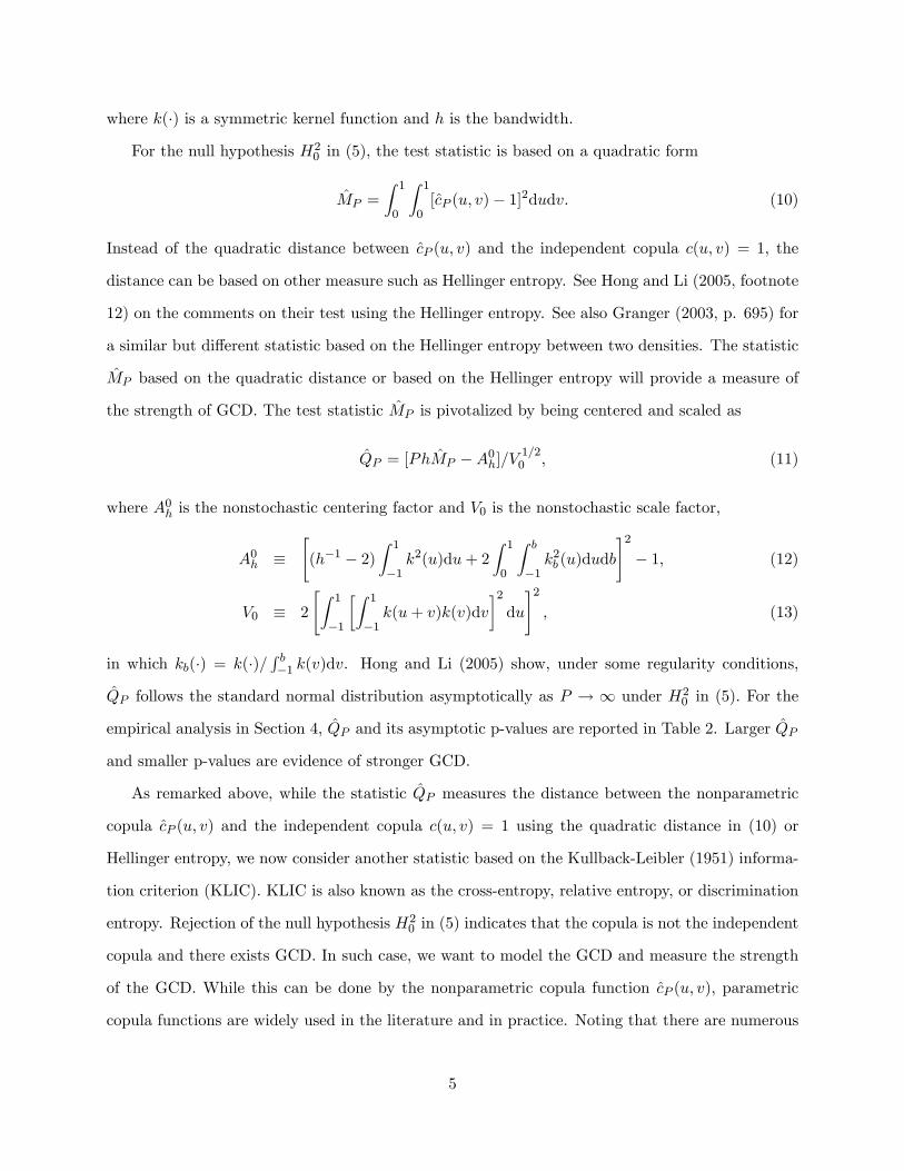
where k(�) is a symmetric kernel function and h is the bandwidth.

For the null hypothesis H20 in (5), the test statistic is based on a quadratic form

MP =

Z 1

0

Z 1

0[cP (u; v)� 1]2dudv: (10)

Instead of the quadratic distance between cP (u; v) and the independent copula c(u; v) = 1; the

distance can be based on other measure such as Hellinger entropy. See Hong and Li (2005, footnote

12) on the comments on their test using the Hellinger entropy. See also Granger (2003, p. 695) for

a similar but di�erent statistic based on the Hellinger entropy between two densities. The statistic

MP based on the quadratic distance or based on the Hellinger entropy will provide a measure of

the strength of GCD. The test statistic MP is pivotalized by being centered and scaled as

QP = [PhMP �A0h]=V1=20 ; (11)

where A0h is the nonstochastic centering factor and V0 is the nonstochastic scale factor,

A0h �"(h�1 � 2)

Z 1

�1k2(u)du+ 2

Z 1

0

Z b

�1k2b (u)dudb

#2� 1; (12)

V0 � 2

"Z 1

�1

�Z 1

�1k(u+ v)k(v)dv

�2du

#2; (13)

in which kb(�) = k(�)=R b�1 k(v)dv. Hong and Li (2005) show, under some regularity conditions,

QP follows the standard normal distribution asymptotically as P ! 1 under H20 in (5). For the

empirical analysis in Section 4, QP and its asymptotic p-values are reported in Table 2. Larger QP

and smaller p-values are evidence of stronger GCD.

As remarked above, while the statistic QP measures the distance between the nonparametric

copula cP (u; v) and the independent copula c(u; v) = 1 using the quadratic distance in (10) or

Hellinger entropy, we now consider another statistic based on the Kullback-Leibler (1951) informa-

tion criterion (KLIC). KLIC is also known as the cross-entropy, relative entropy, or discrimination

entropy. Rejection of the null hypothesis H20 in (5) indicates that the copula is not the independent

copula and there exists GCD. In such case, we want to model the GCD and measure the strength

of the GCD. While this can be done by the nonparametric copula function cP (u; v); parametric

copula functions are widely used in the literature and in practice. Noting that there are numerous

5

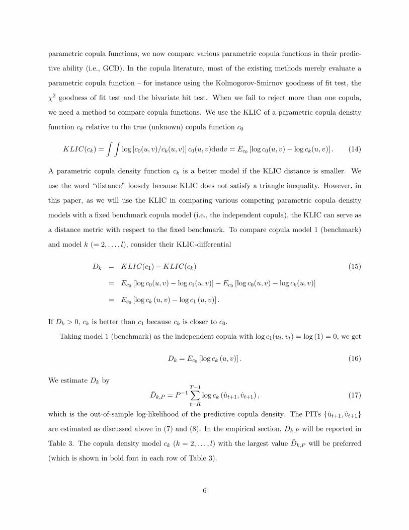
parametric copula functions, we now compare various parametric copula functions in their predic-

tive ability (i.e., GCD). In the copula literature, most of the existing methods merely evaluate a

parametric copula function { for instance using the Kolmogorov-Smirnov goodness of �t test, the

�2 goodness of �t test and the bivariate hit test. When we fail to reject more than one copula,

we need a method to compare copula functions. We use the KLIC of a parametric copula density

function ck relative to the true (unknown) copula function c0

KLIC(ck) =

Z Zlog [c0(u; v)=ck(u; v)] c0(u; v)dudv = Ec0 [log c0(u; v)� log ck(u; v)] : (14)

A parametric copula density function ck is a better model if the KLIC distance is smaller. We

use the word \distance" loosely because KLIC does not satisfy a triangle inequality. However, in

this paper, as we will use the KLIC in comparing various competing parametric copula density

models with a �xed benchmark copula model (i.e., the independent copula), the KLIC can serve as

a distance metric with respect to the �xed benchmark. To compare copula model 1 (benchmark)

and model k (= 2; : : : ; l); consider their KLIC-di�erential

Dk = KLIC(c1)�KLIC(ck) (15)

= Ec0 [log c0(u; v)� log c1(u; v)]� Ec0 [log c0(u; v)� log ck(u; v)]

= Ec0 [log ck (u; v)� log c1 (u; v)] :

If Dk > 0; ck is better than c1 because ck is closer to c0:

Taking model 1 (benchmark) as the independent copula with log c1(ut; vt) = log (1) = 0; we get

Dk = Ec0 [log ck (u; v)] : (16)

We estimate Dk by

�Dk;P = P�1

T�1Xt=R

log ck (ut+1; vt+1) ; (17)

which is the out-of-sample log-likelihood of the predictive copula density. The PITs fut+1; vt+1g

are estimated as discussed above in (7) and (8). In the empirical section, �Dk;P will be reported in

Table 3. The copula density model ck (k = 2; : : : ; l) with the largest value �Dk;P will be preferred

(which is shown in bold font in each row of Table 3).

6

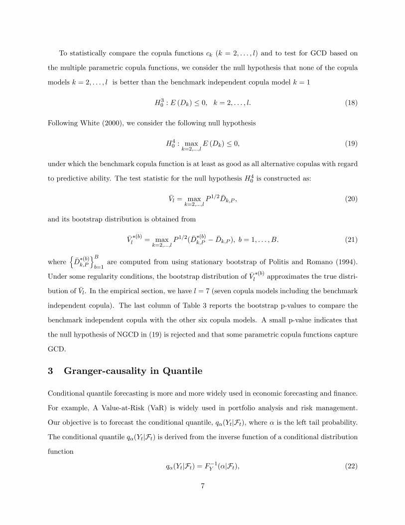
To statistically compare the copula functions ck (k = 2; : : : ; l) and to test for GCD based on

the multiple parametric copula functions, we consider the null hypothesis that none of the copula

models k = 2; : : : ; l is better than the benchmark independent copula model k = 1

H30 : E (Dk) � 0; k = 2; : : : ; l: (18)

Following White (2000), we consider the following null hypothesis

H40 : max

k=2;:::;lE (Dk) � 0; (19)

under which the benchmark copula function is at least as good as all alternative copulas with regard

to predictive ability. The test statistic for the null hypothesis H40 is constructed as:

�Vl = maxk=2;:::;l

P 1=2 �Dk;P ; (20)

and its bootstrap distribution is obtained from

�V�(b)l = max

k=2;:::;lP 1=2( �D

�(b)k;P � �Dk;P ); b = 1; : : : ; B: (21)

wheren�D�(b)k;P

oBb=1

are computed from using stationary bootstrap of Politis and Romano (1994).

Under some regularity conditions, the bootstrap distribution of �V�(b)l approximates the true distri-

bution of �Vl. In the empirical section, we have l = 7 (seven copula models including the benchmark

independent copula). The last column of Table 3 reports the bootstrap p-values to compare the

benchmark independent copula with the other six copula models. A small p-value indicates that

the null hypothesis of NGCD in (19) is rejected and that some parametric copula functions capture

GCD.

3 Granger-causality in Quantile

Conditional quantile forecasting is more and more widely used in economic forecasting and �nance.

For example, A Value-at-Risk (VaR) is widely used in portfolio analysis and risk management.

Our objective is to forecast the conditional quantile, q�(YtjFt), where � is the left tail probability.

The conditional quantile q�(YtjFt) is derived from the inverse function of a conditional distribution

function

q�(YtjFt) = F�1Y (�jFt); (22)

7

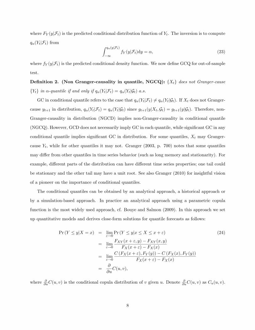
where FY (yjFt) is the predicted conditional distribution function of Yt. The inversion is to compute

q�(YtjFt) from Z q�(yjFt)

�1fY (yjFt)dy = �; (23)

where fY (yjFt) is the predicted conditional density function. We now de�ne GCQ for out-of-sample

test.

De�nition 2. (Non Granger-causality in quantile, NGCQ): fXtg does not Granger-cause

fYtg in �-quantile if and only if q�(YtjFt) = q�(YtjGt) a:s:

GC in conditional quantile refers to the case that q�(YtjFt) 6= q�(YtjGt). If Xt does not Granger-

cause yt+1 in distribution, q�(YtjFt) = q�(YtjGt) since gt+1(yjXt;Gt) = gt+1(yjGt). Therefore, non-

Granger-causality in distribution (NGCD) implies non-Granger-causality in conditional quantile

(NGCQ). However, GCD does not necessarily imply GC in each quantile, while signi�cant GC in any

conditional quantile implies signi�cant GC in distribution. For some quantiles, Xt may Granger-

cause Yt; while for other quantiles it may not. Granger (2003, p. 700) notes that some quantiles

may di�er from other quantiles in time series behavior (such as long memory and stationarity). For

example, di�erent parts of the distribution can have di�erent time series properties; one tail could

be stationary and the other tail may have a unit root. See also Granger (2010) for insightful vision

of a pioneer on the importance of conditional quantiles.

The conditional quantiles can be obtained by an analytical approach, a historical approach or

by a simulation-based approach. In practice an analytical approach using a parametric copula

function is the most widely used approach, cf. Bouye and Salmon (2009). In this approach we set

up quantitative models and derives close-form solutions for quantile forecasts as follows:

Pr (Y � yjX = x) = lim"!0

Pr (Y � yjx � X � x+ ") (24)

= lim"!0

FXY (x+ "; y)� FXY (x; y)FX(x+ ")� FX(x)

= lim"!0

C (FX(x+ "); FY (y))� C (FX(x); FY (y))FX(x+ ")� FX(x)

=@

@uC(u; v);

where @@uC(u; v) is the conditional copula distribution of v given u. Denote

@@uC(u; v) as Cu(u; v).

8

q�(YtjFt) is computed by solving the equation

Cu (FX(xt+1); FY (q�(YtjFt)) = �: (25)

To evaluate predictive ability of those quantile forecasting models q�(YtjFt) obtained from seven

(l = 7) copula functions for C(u; v); we use the \check" loss function of Koenker and Bassett (1978).

The check loss function is a special case in a family of quasi-likelihood functions (Komunjer 2005),

and can be used to measure the lack-of-�t of a quantile forecasting model. The expected check loss

for a quantile forecast q�(YtjFt) at a given � is

Q(�) = E [�� 1(Yt � q�(YtjFt) < 0)] (Yt � q�(YtjFt)) : (26)

As seven copula functions are considered for C(u; v); denote them as Ck(u; v) (k = 1; : : : ; l = 7):

For each copula distribution function Ck(u; v); denote also the corresponding quantile forecast as

q�;k(YtjFt) and its expected check loss as Qk(�). To compare copula model 1 (benchmark) and

model k (= 2; : : : ; l); consider their check loss-di�erential

Dk = Q1 (�)�Qk (�) : (27)

We estimate Dk by

�Dk;P = Q1;P (�)� Qk;P (�) ; (28)

where

Qk;P (�) =1

P

T�1Xt=R

[�� 1(Yt � q�(YtjFt) < 0)] (Yt � q�(YtjFt)) ; k = 1; : : : ; l: (29)

The conditional quantile forecasts from using the copula distribution function Ck (k = 2; : : : ; l)

with the largest value �Dk;P will be preferred.

To statistically compare the conditional quantile forecast q�;k(YtjFt) (k = 2; : : : ; l) and to test

for GCQ based on the multiple parametric copula functions, we consider the null hypothesis of

NGCQ that none of the conditional quantile forecasts computed from copula Ck (k = 2; : : : ; l) is

better than the benchmark quantile forecast computed from the independent copula distribution

C1

H50 : E (Dk) � 0; k = 2; : : : ; l: (30)

9

Following White (2000), we consider the following null hypothesis

H60 : max

k=2;:::;lE (Dk) � 0; (31)

under which the benchmark quantile forecast is at least as good as all alternative conditional

forecasts with regard to the check loss. The test statistic for the null hypothesis H60 is constructed

as:

�Vl = maxk=2;:::;l

P 1=2 �Dk;P : (32)

The bootstrap p-value of this statistic is computed in the same way that we discussed for the KLIC

based test for GCD in the previous section. Compute

�V�(b)l = max

k=2;:::;lP 1=2( �D

�(b)k;P � �Dk;P ); b = 1; : : : ; B: (33)

wheren�D�(b)k;P

oBb=1

are computed from using the stationary bootstrap of Politis and Romano (1994).

Under some regularity conditions, the bootstrap distribution of �V�(b)l approximates the true distri-

bution of �Vl. In the empirical section, we have l = 7 (seven copula models including the benchmark

independent copula). The null hypothesis of NGCQ in (31) is that none of the six copula models

(for GCQ) can produce better quantile forecasts than the Independent copula (for NGCQ). Each

cell of Table 4 reports the bootstrap p-values to compare the benchmark quantile forecast with the

other six quantile forecasts for a value of � and for a subsample. A small p-value indicates that the

null hypothesis is rejected and that some parametric copula functions capture GCQ with better

quantile forecast of Y by conditioning on X.

4 Empirical Analysis

We investigate the causality and dependence between a pair of two �nancial markets using a copula-

based approach. We focus on pair-wise causal relationships between three major stock markets of

US, Japan, and UK. In particular, we compare multiple copula functions with Independent copula

function, in order to test GCD and GCQ, of one market's return conditional on another market's

return.

The data used in our empirical applications are the daily return on the S&P500 stock index

(S&P500), the NIKKEI 225 stock index (NIKKEI) and FTSE 100 stock index (FTSE) from Jan. 3,

10

1995 to Dec. 31, 2005. The source of the data is Yahoo Finance. To analyze the causal e�ects, we

only keep the observations of the date when all three markets were open. The total observations in

the data sets are 2566. Approximately, there are 230-240 observations per year and 20 observations

per month.

On the same trading day, trading in the Tokyo Stock Exchange and London Stock Exchange

precedes that in the New York Stock Exchange. To explore the causality among those �nancial

markets, we use four data sets, which include stock returns on NIKKEI and S&P500 (same day)

(referred to as \Japan-US"), stock returns on FTSE and S&P500 (same day) (referred to as \UK-

US"), returns on S&P500 and next day's NIKKEI (referred to as \US-Japan"), and returns on

S&P500 and next day's FTSE (referred to as \US-UK"), respectively.

To simplify the notation, in all four data sets, we use fXtg to denote the preceding variable and

fYtg as the trailing variable. For instance, in the data set of same day's stock returns on NIKKEI

and S&P500, fXtg denotes stock returns on the NIKKEI and fYtg denotes stock returns on the

S&P500. Panel A of Table 1 reports detailed information of variables in those data sets.1

The focus of empirical study is out-of-sample forecasting. Hence, for each subsample, we choose

5 years (about T = 1170 observations), in which 3 years data (about R = 700 observations) are

used for in-sample estimation of the models and 2 years data (about P = 470 observations) are

used for out-of-sample forecasting, of daily series. To conduct a robustness check and to explore

the causality over time, the subsample shifts forward by 1 year. Therefore, there are altogether 7

subsamples. Details on the subsamples are listed in Panel B of Table 1.

In recent years, multivariate GARCH models are widely applied to model and forecast the tem-

poral dependence and correlation between �nancial markets. Rather than assuming the bivariate

normal distribution as in most multivariate models, we use a copula distribution. Because we are

interested in testing GCD and GCQ instead of modeling the correlation between �nancial returns,

we apply a relatively simple model in which the two univariate processes are modelled by a GARCH

model and the dependence structure is modelled by a copula.

1Exchange rate uctuations would in uence stock market returns dominated by the US dollar in Japan and Britain.To remove the possible in uence of such impacts, we also analyze causality between di�erent �nancial markets usingforeign exchange rate adjusted returns. We also study the same four data sets, but with USD dominated returns.The data source of the daily exchange rate of the Yen/USD and USD/GBP is the FERD database of Federal Reserveof St. Luis. As the results were basically the same, we do not report this FX-adjusted results but they are availableupon request.

11

Let fXtg and fYtg be stock returns with zero mean (or demeaned). The estimation procedure

is in two-steps following Chen and Fan (2006b). In the �rst step the univariate conditional variance

for fXtg and fYtg respectively is modeled by a univariate GARCH process, i.e.,

h�1=2x;t Xt � N(0; 1); (34)

hx;t = �x0 + �x1x2t�1 + �x2hx;t�1;

h�1=2y;t Yt � N(0; 1); (35)

hy;t = �y0 + �y1y2t�1 + �y2hy;t�1;

In the second step the joint distribution is modeled by a copula function�h�1=2x;t Xt; h

�1=2y;t Yt

�� C(u; v): (36)

By choosing di�erent copula functions and marginal distributions, this model can capture various

dependence structure between �nancial time series. The model is estimated by a two-stage quasi

maximum likelihood (QML) method. In the �rst stage, we estimate the two univariate GARCH

models by QML method. With the estimated parameters in the GARCH model, the PIT values

of the two marginal processes fut; vtg are estimated by the EDFs as in (7) and (8). In the second

stage, we estimate the copula parameters following Chen and Fan (2006b).

4.1 Granger-causality in Distribution

We apply the proposed out-of-sample test for GCD following Hong and Li (2005). As discussed in

Section 2, we actually test H0 : c(u; v) = 1: The forecasted conditional variance for fXtg and fYtg;

hx;t+1 and hy;t+1, are computed by

hx;t+1 = �x0 + �x1x2t + �x2ht;x; (37)

hy;t+1 = �y0 + �y1y2t + �y2ht;y; (38)

Thus forecasted CDF values ut+1 and vt+1 for xt+1 and yt+1 are calculated by the empirical dis-

tribution function (EDF). A nonparametric copula function is estimated with paired EDF values

fut+1; vt+1gT�1t=R using product kernel functions. We use a quartic kernel in the boundary kernel

function speci�ed in Section 2, which is speci�ed as

k(u) =15

16(1� u2)21(juj � 1): (39)

12

For simplicity, bandwidths for u and v are assumed to be the same. Following Hong and Li (2005),

we set h = �R�1=6, where � is the standard error of ut+1: This assumption can be relaxed and the

results are not greatly a�ected.

In Table 2, we report the GCD results using the Hong and Li test statistic for fxt+1; yt+1gT�1t=R ;

computed by the method discussed in Section 2. We �nd signi�cant GCD between all pairs of three

�nancial markets. With the shift of subsamples, the GCD remains signi�cant for all subsamples and

data sets. Not only the foreign stock markets Granger-causes the US stock market, the information

of the US market also a�ects the foreign markets in the following day. This �nding is consistent

with the literature on Granger-causality in variance between �nancial markets, e.g., Cheung and

Ng (1996), Hong (2001), Sensier and van Dijk (2004).

The rejection of the null hypothesis that the copula is independent, H0 : c (u; v) = 1; leads us

to consider various parametric copula density functions. In the literature, Gaussian copulas, Frank

copulas, Clayton copulas, Clayton Survival copulas and Gumbel copulas and Gumbel Survival cop-

ulas are the most commonly used copula functions. We use these copula functions (see Appendix).

Speci�cally, we form the forecasted copula density function is c(u; v). Based on the decomposition

theorem of a bivariate density in (43), the log-likelihood of a bivariate density is decomposed as

log fXY (x; y) = log fX(x) + log fY (y) + log c (FX(x); FY (y)) ; (40)

Noting that we use the same marginal processes for all copula models, to compare predictive

log-likelihood is equivalent to compare log c(ut+1; vt+1), where ut+1 and vt+1 are computed using

empirical distribution functions. Results are reported in Table 3. The independent copula is clearly

rejected for all seven subsamples and all four data sets. This �nding is consistent with the Hong-Li

test results for GCD in Table 2.

For Data Set 1A (Japan-US), the Clayton copula and the Gumbel Survival copula are the best

two copulas, both of which exhibit increasing dependence in the lower tails. See Appendix on

some properties of copulas. These two copula clear dominates the mirror counterparts, Clayton

Survival copula and Gumbel copula, which have much smaller log-likelihood. The other data sets

show similar pattern. In general, the best copula functions are Clayton or Gumbel Survival (both

capture the left tail dependence). Even when the Gaussian copula is the best for some subsamples,

13

Clayton or Gumbel Survival still dominate Clayton Survival or Gumbel in almost all cases (of the

seven subsamples and four data sets).

This comparison of the copula only tells that left (lower) tail dependence is stronger than the

right (upper) tail dependence. It does not mean that the upper tail dependence does not exist. In

fact many cases show that the symmetric copula, namely Gaussian copula and the Frank copula

are selected as the best copula function. The comparison of the copulas simply show that the bad

news are generally more contagious than good news, but it does not show whether or not good

news may Granger-cause the other market. In order to examine this, we need to examine the

Granger-causality in various quantiles, GCQ, which we do next.

4.2 Granger-causality in Quantiles

As discussed in Section 3, signi�cant GCD does not imply Granger-causality in each conditional

quantile. In our empirical study, we focus on three regions of the distribution - the left tail (1% quan-

tile, 5% quantile and 10% quantile), the central region (40% quantile, median and 60% quantile) and

the right tail (90% quantile, 95% quantile and 99% quantile). We compare the Granger-causality

in those quantiles. To forecast the conditional quantile for yt+1, because xt+1 precedes yt+1, xt+1

is a realized value thus can be used in forecasting conditional quantile q�(yt+1jxt+1). For instance,

before the New York Stock Exchange opens, the Tokyo Stock Exchange has closed.

We compute the quantile forecasts by inverting the conditional copula distribution, as described

in Section 3. We use six copulas { Gaussian, Frank, Clayton, Clayton Survival, Gumbel and Gumbel

Survival copulas. These copula functions represent di�erent dependence structures. We compare

the check loss functions to evaluate predictive ability of di�erent quantile forecasting copula models

relative to the quantile forecasts without GCQ.2 The quantile forecasts without GCQ is computed

from the marginal distribution of y; which is equivalent to the quantile forecast from using the

Independent copula. The null hypothesis of the Reality Check test is that none of these six copula

models (which models GCQ) makes better quantile forecast than the Independent copula (without

GCQ). The results of testing GCQ in p-values are reported in Table 4. The small p-values of the

2We also use the loss functions proposed by Komunjer (2005) with p = 1; 3; and 5 respectively. Results usingloss functions by Komunjer (2005) mimic those using a check loss function. Therefore, we only report results usinga check loss function.

14

Reality Check in Table 4 indicate the rejection of the null hypothesis, indicating that there exists

a copula function to model GCQ and makes better quantile forecast of Y by conditioning on X.

We report several interesting �ndings.

1. First, in every data set, a quantile forecasting model with no Granger-causality in quantile

is rejected in many � quantiles, verifying the �nding of signi�cant GCD between �nancial

markets. Meanwhile, for some regions, the quantile forecast model with non-Granger-causality

can not be rejected. This in part veri�es that GCD does not necessarily imply Granger-

causality in every quantile.

2. The GCQ between US and Japan shows di�erent patterns in Data Set 1A (Japan-US) than

Data Set 1B (US-Japan). Data Set 1A (Japan-US) does not show many small p-values,

indicating the Japanese stock market does not Granger-cause the US market in most quantiles.

The Reality Check p-values for Data Set 1B (US-Japan) are very small across almost entire

quantiles for all subsamples, indicating the US stock market strongly Granger-causes the

Japanese stock market in all quantiles, left tail (bad performance), center (usual performance),

and right tail (good performance) of the distribution of the NIKKEI returns conditional on

the yesterday's S&P500 returns. So there is clear asymmetry between US and Japan stock

markets in GCQ.

3. It is interesting to see that the same asymmetry is not found between US and UK stock

markets in GCQ. Looking at Panels C and D of Table 4, it is seen that there are small p-

values all over the places (across the quantiles and over di�erent subsamples). GCQ is clear

in both directions, from UK to US and also from US to UK markets, in all quantiles. GCQ is

asymmetric between US and Japan �nancial markets, but more symmetric between US and

UK markets. However, the results of Tables 2, 3, 4 suggest that the causality is even stronger

from UK to US than from US to UK, although it is statistically signi�cant in both directions.

5 Conclusions

Instead of testing Granger-causality in conditional mean or conditional variance, we consider testing

for GCD by checking for independence in the copula function. Among the returns in three major

15

stock markets, we �nd signi�cant GCD. We also estimate several copula functions to model the

GCD between �nancial markets, and invert the estimated conditional copula distribution function

to obtained the conditional quantile functions, which enable us to examine the Granger-causality

in various quantiles. We �nd that causality to the US stock market is more signi�cant from UK

than from Japan, while causality from the US stock market to UK and Japan stock markets is

signi�cant almost equally or slightly more to Japan than to UK.

The literature on GCQ is young and thin. The �rst paper on GCQ is Lee and Yang (2012), who

explore money-income Granger causality in the conditional quantile and �nd that GCQ is signi�cant

in tail quantiles whereas it is not signi�cant near the middle quantiles of the conditional distribution.

Lee and Yang (2012) use the quantile regression to compute the out-of-sample quantile forecasts.

While not reported in the paper for space, we have also computed the quantile forecasts from the

quantile regressions instead of inverting the conditional copula functions. The results showed that

the inverting conditional copula distribution is the superior approach to the quantile regressions

especially towards both tails. Even in the middle of the distribution, the quantile regression was

often dominated by the copula approach. This result was robust with all subsamples and data

sets. This indicates that using a copula based approach has great potential to improve the quantile

forecasting especially in the tails (such as VaRs) and perhaps even in the center of the distribution.

Another advantage of inverting the conditional copula functions to obtain quantile forecasts instead

of using the regression quantiles is that the former can avoid entirely the quantile-crossing problem

while the latter methods requires some correction or adjustment as studied by Chernozhukov et

al (2009). Jeong et al (2012) consider a nonparametric test for in-sample GCQ and examines the

causal relations between the crude oil price, the USD/GBP exchange rate, and the gold price in

the gold market.

The contribution of the current paper is two fold. First, we show how to test for GCD using the

copula function and how to compare di�erent parametric copula functions. These methods are based

on quadratic distance or Hellinger entropy, and on the KLIC cross-entropy. The distance or entropy

provides measures of the strength in GCD, as shown in Section 2. Second, we then show how to

invert the predictive conditional copula functions to obtain conditional quantile forecasts and how

to test for the out-of-sample GCQ, as shown in Section 3. Ashley, Granger and Schmalensee (1980)

16

advocate that a test for Granger-causality of X for Y be conducted for out-of-sample predictive

content of the conditioning variable X for Y:

6 Appendix: Copula

In the framework of time series, a conditional copula is more often applied than a unconditional

copula. As in Patton (2006b), we de�ne the conditional copula as follows.

Sklar's Theorem for Conditional Copula: Let FXY (x; y) be a bivariate conditional joint

distribution function with conditional margin distributions FX(x) and FY (y). Then there exists a

conditional copula function C such that for all x, y

FXY (x; y) = C(FX(x); FY (y)); (41)

where FX(x) = Pr (X � xjFt) ; FY (y) = Pr (Y � yjFt) :

There are two important corollaries to this theorem:

Representation of Conditional Copula functions: The bivariate conditional copula function

can be obtained from the bivariate conditional joint distribution function FXY (x; y) by the following:

C(u; v) = FXY�F�1X (u); F�1Y (v)

�(42)

where u = FX(x) and v = FY (y).

Decomposition of Bivariate Density: Let fXY (x; y) =@2FXY (x;y)

@x@y , fX(x) =@FX(x)@x ; and

fY (y) =@FY (y)@y . Then

fXY (x; y) = fX(x)� fY (y)� c (FX(x); FY (y)) ; (43)

where c(u; v) = @2C(u;v)@u@v is the conditional copula density function.

Some parametric copula functions are widely used, such as Gaussian copula, Student-t cop-

ula, Frank copula, Clayton copula, Gumbel copula, Gumbel Survival copula and Clayton survival

copula. We use the following seven copula functions in this paper.

(1) Gaussian copula

CGaussian(u; v; �) =

Z ��1(u)

�1

Z ��1(v)

�1

1

2�p1� �2

exp

�r

2 + s2 � 2�rs2(1� �2)

!drds; � 2 (�1; 1) :

17

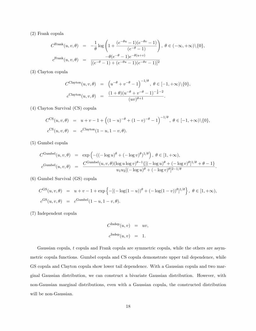
(2) Frank copula

CFrank(u; v; �) = �1�log

1 +

(e��u � 1)(e��v � 1)(e�� 1)

!; � 2 (�1;+1)nf0g;

cFrank(u; v; �) =��(e�� 1)e��(u+v)

[(e�� 1) + (e��u � 1)(e��v � 1)]2

(3) Clayton copula

CClayton(u; v; �) =�u�� + v�� 1

��1=�; � 2 [�1;+1)nf0g;

cClayton(u; v; �) =(1 + �)(u�� + v�� 1)� 1

��2

(uv)�+1:

(4) Clayton Survival (CS) copula

CCS(u; v; �) = u+ v � 1 +�(1� u)�� + (1� v)�� 1

��1=�; � 2 [�1;+1)nf0g;

cCS(u; v; �) = cClayton(1� u; 1� v; �):

(5) Gumbel copula

CGumbel(u; v; �) = exp��((� log u)� + (� log v)�)1=�

�; � 2 [1;+1);

cGumbel(u; v; �) =CGumbel(u; v; �)(log u log v)��1f[(� log u)� + (� log v)�]1=� + � � 1g

u1u2[(� log u)� + (� log v)�]2�1=�:

(6) Gumbel Survival (GS) copula

CGS(u; v; �) = u+ v � 1 + expn�[(� log(1� u))� + (� log(1� v))�]1=�

o; � 2 [1;+1);

cGS(u; v; �) = cGumbel(1� u; 1� v; �):

(7) Independent copula

CIndep(u; v) = uv;

cIndep(u; v) = 1:

Gaussian copula, t copula and Frank copula are symmetric copula, while the others are asym-

metric copula functions. Gumbel copula and CS copula demonstrate upper tail dependence, while

GS copula and Clayton copula show lower tail dependence. With a Gaussian copula and two mar-

ginal Gaussian distribution, we can construct a bivariate Gaussian distribution. However, with

non-Gaussian marginal distributions, even with a Gaussian copula, the constructed distribution

will be non-Gaussian.

18

References

Ang, A. and J. Chen (2002), \Asymmetric Correlations of Equity Portfolios", Review of Financial

Studies 63, 443-494.

Ashley, R., C.W.J. Granger, and R. Schmalensee, (1980), \Advertising and Aggregate Consump-

tion: An Analysis of Causality", Econometrica 48, 1149-1167.

Bouye, E. and M. Salmon (2009), \Copula Quantile Regressions and Tail Area Dynamic Depen-

dence in Forex Markets," The European Journal of Finance 15, 721-750.

Chen, X. and Y. Fan (2005), \Pseudo-likelihood Ratio Tests for Semiparametric Multivariate

Copula Model Selection", The Canadian Journal of Statistics 33(3), 389-414.

Chen, X. and Y. Fan (2006a), \Estimation of Copula-Based Semiparametric Time Series Models",

Journal of Econometrics 130(2), 307-335.

Chen, X. and Y. Fan (2006b), \Estimation and Model Selection of Semiparametric Copula-based

Multivariate Dynamic Models under Copula Misspeci�cation" Journal of Econometrics 135,

125-154.

Chernozhukov, V., I. Fernandez-Val and A. Galichon (2009), \Improving point and interval esti-

mators of monotone functions by rearrangement," Biometrika 96(3), 559-575.

Cheung, Y.-W. and L.K. Ng (1996), \A Causality-in-Variance Test and its Application to Financial

Market Prices", Journal of Econometrics 72, 33-48.

Comte, F. and O. Lieberman (2000), \Second Order Noncausality in Multivariate GARCH Processes",

Journal of Time Series Analysis 21, 535-557.

Dufour, J. and E. Renault (1998), \Short Run and Long Run Causality in Time Series: Theory",

Econometrica 66, 1099-1125.

Dufour, J., D. Pelletier and E. Renault (2006), \Short Run and Long Run Causality in Time

Series: Inference", Journal of Econometrics 132, 337-362.

Embrechts, P., A. Hoing and A. Juri (2003), \Using Copulae to Bound the Value-at-Risk for

Functions of Dependent Risks", Finance and Stochastics 7(2), 145-167.

Granger, C.W.J. (1969), \Investigating Causal Relations by econometric Models and Cross-

Spectral Methods", Econometrica 37, 424-438.

Granger, C.W.J. (1980), \Testing for Causality: A Personal Viewpoint", Journal of Economic

Dynamics and Control 2, 329-352.

Granger, C.W.J. (1988), \Some Recent Developments in a Concept of Causality", Journal of

Econometrics 39, 199-211.

19

Granger, C.W.J. (2003), \Time Series Concepts for Conditional Distributions," Oxford Bulletin

of Economics and Statistics 65, 689-701.

Granger, C.W.J. (2010), \Some Thoughts on the Development of Cointegration", Journal of

Econometrics 158, 3-6.

Granger, C.W.J., R.P. Robins and R.F. Engle (1986). \Wholesale and Retail Prices: Bivariate

Time Series Modelling with Forecastable Error Variances", in: D. Belsley and E. Kuh, eds.,

Model Reliability, MIT Press, Cambridge, MA, 117.

Granger, C.W.J., T. Ter�asvitra and A. Patton (2006), \Common Factors in Conditional Distrib-

utions for Bivariate Time Series", Journal of Econometrics 132 (1), 43-57.

Hansen, P.R. (2005), \A Test for Superior Predictive Ability," Journal of Business and Economic

Statistics 23, 365-380.

Hong, Y. (2001), \A Test for Volatility Spillover with Application to Exchange Rates", Journal

of Econometrics 103, 183-224.

Hong, Y., and H. Li (2005), \Nonparametric Speci�cation Testing for Continuous-Time Models

with Applications to Term Structure of Interest Rates", Review of Financial Studies 18, 37-84.

Jeong, K., W.K. H�ardle and S. Song (2012), \A Consistent Nonparametric Test for Causality in

Quantile" Econometric Theory 28(4), 861-887.

Koenker, R and G. Basset (1978), \Asymptotic Theory of Least Absolute Error Regression",

Journal of the American Statistical Association 73, 618-622.

Komunjer, I. (2005), \Quasi-Maximum Likelihood Estimation for Conditional Quantiles", Journal

of Econometrics 128(1), 137-164.

Kullback, L. and R.A. Leibler (1951), \On Information and Su�ciency", Annals of Mathematical

Statistics 22, 79-86.

Lee, T.-H. and W. Yang (2012), \Money-Income Granger-Causality in Quantiles", Advances in

Econometrics, Volume 30, Chapter 12, pp. 383-407, Millimet, D. and Terrell, D. (ed.), Emer-

ald Publishers.

Li, D.X. (2000), \On Default Correlation: A Copula Function Approach", Journal of Fixed Income

9(4), 43-54.

Lin, W.L., R.F. Engle and T. Ito (1994), Do Bulls and Bears Move Across Borders? International

transmission stock returns and volatility, Review of Financial Studies 7, 507-538.

Patton, A.J. (2006a), \Estimation of Multivariate Models for Time Series of Possibly Di�erent

Lengths", Journal of Applied Econometrics 21(2), 147-173.

20

Patton, A.J. (2006b), \Modelling Asymmetric Exchange Rate Dependence", International Eco-

nomic Review 47(2), 527-556.

Politis, D.N. and J.P. Romano (1994), \The Stationary Bootstrap", Journal of the American

Statistical Association 89, 1303-1313.

Scaillet, O. and J.D. Fermanian (2003), \Nonparametric Estimation of Copulas for Time Series",

Journal of Risk 5, 25-54.

Sensier, M. and D. van Dijk (2004), \Testing for Volatility Changes in US Macroeconomic Time

Series", Review of Economics and Statistics 86, 833-839.

Sims, C.A. (1972), \Money, Income and Causality", American Economic Review 62, 540-542.

Sims, C.A. (1980), \Comparison of Interwar and Postwar Business Cycles: Monetarism Reconsid-

ered", American Economic Review 70, 250-259.

Stock, J.H. and M.W. Watson (1989), \Interpreting the Evidence on Money-Income Causality",

Journal of Econometrics 40, 161-181.

White, H. (2000), \A Reality Check for Data Snooping", Econometrica 68, 1097-1126.

21

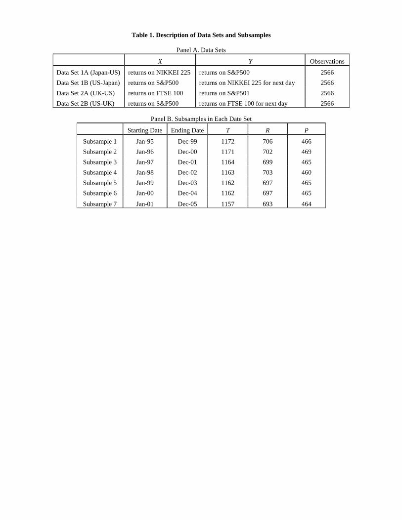
Table 1. Description of Data Sets and Subsamples

Panel A. Data Sets

X Y Observations

Data Set 1A (Japan-US) returns on NIKKEI 225 returns on S&P500 2566 Data Set 1B (US-Japan) returns on S&P500 returns on NIKKEI 225 for next day 2566 Data Set 2A (UK-US) returns on FTSE 100 returns on S&P501 2566 Data Set 2B (US-UK) returns on S&P500 returns on FTSE 100 for next day 2566

Panel B. Subsamples in Each Date Set

Starting Date Ending Date T R P

Subsample 1 Jan-95 Dec-99 1172 706 466 Subsample 2 Jan-96 Dec-00 1171 702 469 Subsample 3 Jan-97 Dec-01 1164 699 465 Subsample 4 Jan-98 Dec-02 1163 703 460 Subsample 5 Jan-99 Dec-03 1162 697 465 Subsample 6 Jan-00 Dec-04 1162 697 465

Subsample 7 Jan-01 Dec-05 1157 693 464

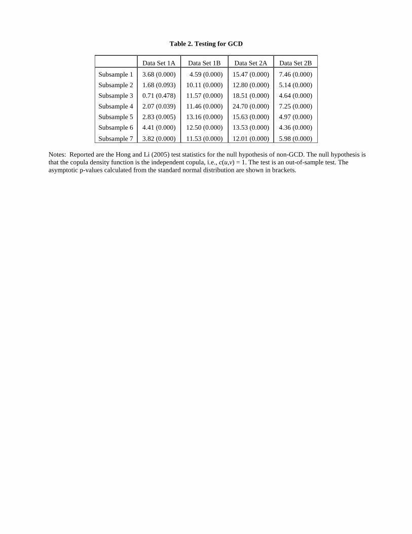
Table 2. Testing for GCD

Data Set 1A Data Set 1B Data Set 2A Data Set 2B

Subsample 1 3.68 (0.000) 4.59 (0.000) 15.47 (0.000) 7.46 (0.000) Subsample 2 1.68 (0.093) 10.11 (0.000) 12.80 (0.000) 5.14 (0.000) Subsample 3 0.71 (0.478) 11.57 (0.000) 18.51 (0.000) 4.64 (0.000) Subsample 4 2.07 (0.039) 11.46 (0.000) 24.70 (0.000) 7.25 (0.000) Subsample 5 2.83 (0.005) 13.16 (0.000) 15.63 (0.000) 4.97 (0.000) Subsample 6 4.41 (0.000) 12.50 (0.000) 13.53 (0.000) 4.36 (0.000)

Subsample 7 3.82 (0.000) 11.53 (0.000) 12.01 (0.000) 5.98 (0.000) Notes: Reported are the Hong and Li (2005) test statistics for the null hypothesis of non-GCD. The null hypothesis is that the copula density function is the independent copula, i.e., c(u,v) = 1. The test is an out-of-sample test. The asymptotic p-values calculated from the standard normal distribution are shown in brackets.

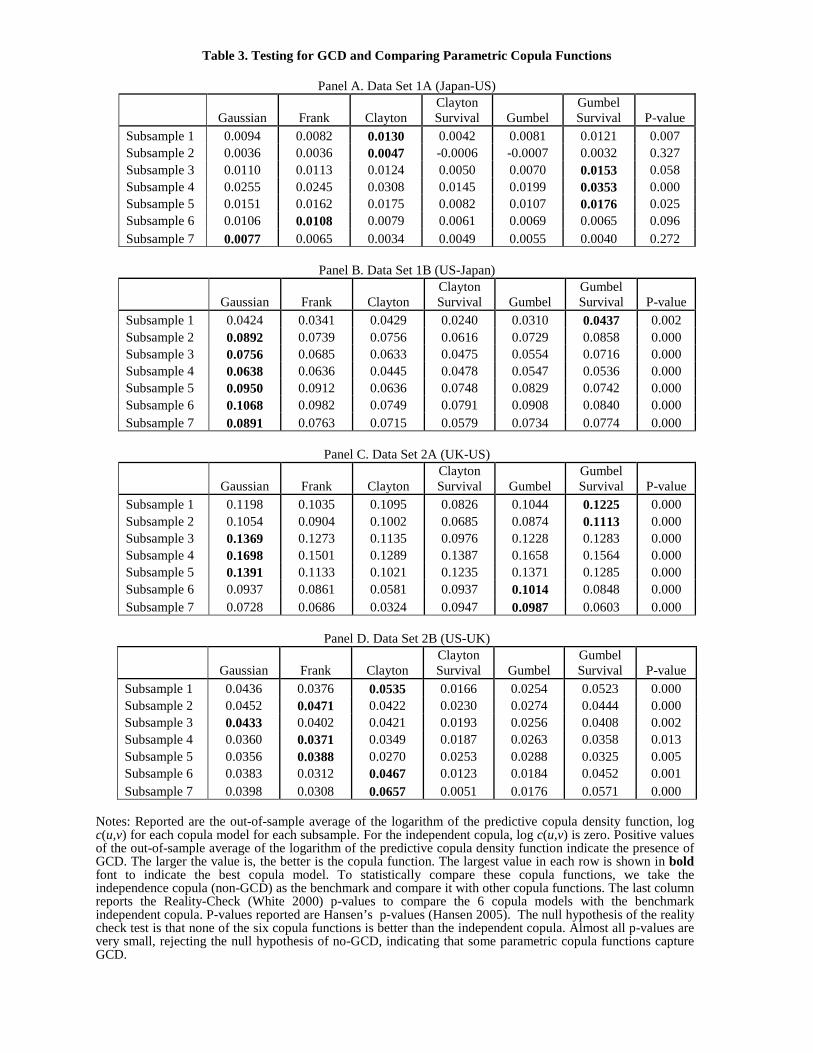
Table 3. Testing for GCD and Comparing Parametric Copula Functions

Panel A. Data Set 1A (Japan-US)

Gaussian Frank Clayton Clayton Survival Gumbel

Gumbel Survival P-value

Subsample 1 0.0094 0.0082 0.0130 0.0042 0.0081 0.0121 0.007 Subsample 2 0.0036 0.0036 0.0047 -0.0006 -0.0007 0.0032 0.327 Subsample 3 0.0110 0.0113 0.0124 0.0050 0.0070 0.0153 0.058 Subsample 4 0.0255 0.0245 0.0308 0.0145 0.0199 0.0353 0.000 Subsample 5 0.0151 0.0162 0.0175 0.0082 0.0107 0.0176 0.025 Subsample 6 0.0106 0.0108 0.0079 0.0061 0.0069 0.0065 0.096 Subsample 7 0.0077 0.0065 0.0034 0.0049 0.0055 0.0040 0.272

Panel B. Data Set 1B (US-Japan)



Subsample 1 0.0424 0.0341 0.0429 0.0240 0.0310 0.0437 0.002 Subsample 2 0.0892 0.0739 0.0756 0.0616 0.0729 0.0858 0.000 Subsample 3 0.0756 0.0685 0.0633 0.0475 0.0554 0.0716 0.000 Subsample 4 0.0638 0.0636 0.0445 0.0478 0.0547 0.0536 0.000 Subsample 5 0.0950 0.0912 0.0636 0.0748 0.0829 0.0742 0.000 Subsample 6 0.1068 0.0982 0.0749 0.0791 0.0908 0.0840 0.000 Subsample 7 0.0891 0.0763 0.0715 0.0579 0.0734 0.0774 0.000

Panel C. Data Set 2A (UK-US)




Panel D. Data Set 2B (US-UK)




Notes: Reported are the out-of-sample average of the logarithm of the predictive copula density function, log c(u,v) for each copula model for each subsample. For the independent copula, log c(u,v) is zero. Positive values of the out-of-sample average of the logarithm of the predictive copula density function indicate the presence of GCD. The larger the value is, the better is the copula function. The largest value in each row is shown in bold font to indicate the best copula model. To statistically compare these copula functions, we take the independence copula (non-GCD) as the benchmark and compare it with other copula functions. The last column reports the Reality-Check (White 2000) p-values to compare the 6 copula models with the benchmark independent copula. P-values reported are Hansen’s p-values (Hansen 2005). The null hypothesis of the reality check test is that none of the six copula functions is better than the independent copula. Almost all p-values are very small, rejecting the null hypothesis of no-GCD, indicating that some parametric copula functions capture GCD.

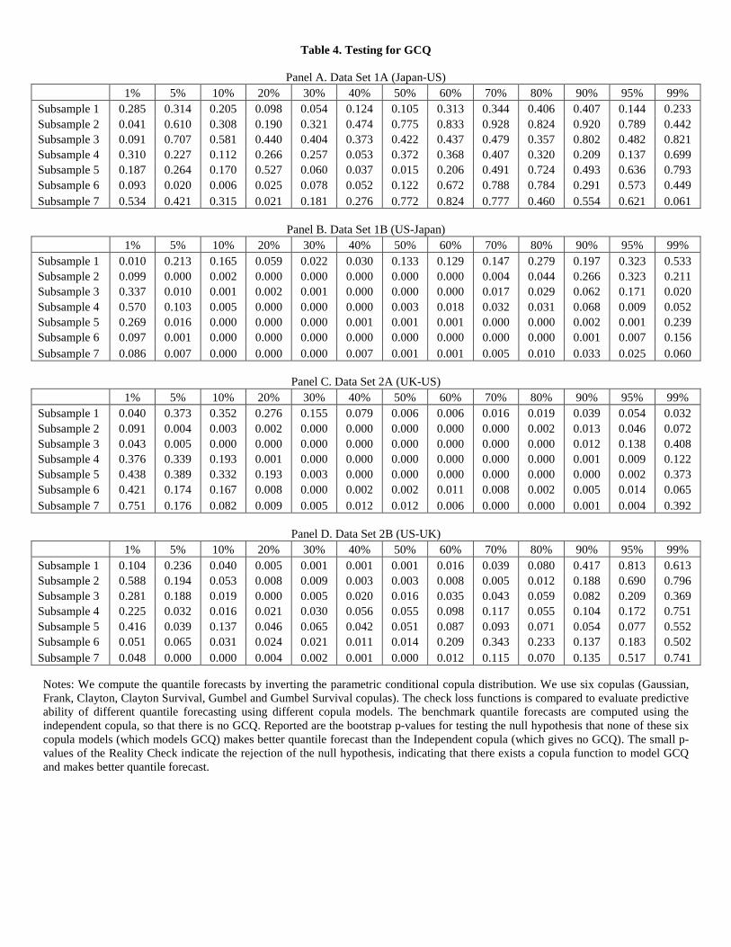
Table 4. Testing for GCQ

Panel A. Data Set 1A (Japan-US) 1% 5% 10% 20% 30% 40% 50% 60% 70% 80% 90% 95% 99%

Subsample 1 0.285 0.314 0.205 0.098 0.054 0.124 0.105 0.313 0.344 0.406 0.407 0.144 0.233 Subsample 2 0.041 0.610 0.308 0.190 0.321 0.474 0.775 0.833 0.928 0.824 0.920 0.789 0.442 Subsample 3 0.091 0.707 0.581 0.440 0.404 0.373 0.422 0.437 0.479 0.357 0.802 0.482 0.821 Subsample 4 0.310 0.227 0.112 0.266 0.257 0.053 0.372 0.368 0.407 0.320 0.209 0.137 0.699 Subsample 5 0.187 0.264 0.170 0.527 0.060 0.037 0.015 0.206 0.491 0.724 0.493 0.636 0.793 Subsample 6 0.093 0.020 0.006 0.025 0.078 0.052 0.122 0.672 0.788 0.784 0.291 0.573 0.449 Subsample 7 0.534 0.421 0.315 0.021 0.181 0.276 0.772 0.824 0.777 0.460 0.554 0.621 0.061

Panel B. Data Set 1B (US-Japan)

1% 5% 10% 20% 30% 40% 50% 60% 70% 80% 90% 95% 99% Subsample 1 0.010 0.213 0.165 0.059 0.022 0.030 0.133 0.129 0.147 0.279 0.197 0.323 0.533 Subsample 2 0.099 0.000 0.002 0.000 0.000 0.000 0.000 0.000 0.004 0.044 0.266 0.323 0.211 Subsample 3 0.337 0.010 0.001 0.002 0.001 0.000 0.000 0.000 0.017 0.029 0.062 0.171 0.020 Subsample 4 0.570 0.103 0.005 0.000 0.000 0.000 0.003 0.018 0.032 0.031 0.068 0.009 0.052 Subsample 5 0.269 0.016 0.000 0.000 0.000 0.001 0.001 0.001 0.000 0.000 0.002 0.001 0.239 Subsample 6 0.097 0.001 0.000 0.000 0.000 0.000 0.000 0.000 0.000 0.000 0.001 0.007 0.156 Subsample 7 0.086 0.007 0.000 0.000 0.000 0.007 0.001 0.001 0.005 0.010 0.033 0.025 0.060

Panel C. Data Set 2A (UK-US)


Panel D. Data Set 2B (US-UK)


Notes: We compute the quantile forecasts by inverting the parametric conditional copula distribution. We use six copulas (Gaussian, Frank, Clayton, Clayton Survival, Gumbel and Gumbel Survival copulas). The check loss functions is compared to evaluate predictive ability of different quantile forecasting using different copula models. The benchmark quantile forecasts are computed using the independent copula, so that there is no GCQ. Reported are the bootstrap p-values for testing the null hypothesis that none of these six copula models (which models GCQ) makes better quantile forecast than the Independent copula (which gives no GCQ). The small p-values of the Reality Check indicate the rejection of the null hypothesis, indicating that there exists a copula function to model GCQ and makes better quantile forecast.

granger-causality in quantiles between financial markets ...taelee/paper/weiping2.pdf · 1...

Documents