granger causality between exports, imports and …1)6y3.pdfcausal links between foreign trade and...

TThhee EEccoonnoommiicc RReesseeaarrcchh GGuuaarrddiiaann –– VVooll.. 22((11))22001122 SSeemmii--aannnnuuaall OOnnlliinnee JJoouurrnnaall,, wwwwww..eeccrrgg..rroo

IISSSSNN:: 22224477--88553311,, IISSSSNN--LL:: 22224477--88553311 Econ Res Guard 2(1): 43-59

EEccoonn RReess GGuuaarrdd 4433 22001122

GRANGER CAUSALITY BETWEEN EXPORTS, IMPORTS AND GDP IN FRANCE: EVIDANCE FROM USING GEOSTATISTICAL MODELS

Arshia Amiri a, b a Department of Agricultural Economics, College of Agriculture, Shiraz University, Shiraz, Iran b GREQAM CNRS - ORS PACA - INSERM U912, Marseille, France E-mail: [email protected]

Ulf-G Gerdtham c, d, e c Department of Economics, Lund University, Sweden d Health Economics & Management, Institute of Economic Research, Lund University, Sweden e Centre for Primary Health Care Research, Lund University, Sweden E-mail: [email protected]

Abstract This paper introduces a new way of investigating linear and nonlinear Granger causality between exports, imports and economic growth in France over the period 1961_2006 with using geostatistical models (kiriging and Inverse distance weighting). Geostatistical methods are the ordinary methods for forecasting the locatins and making map in water engineerig, environment, environmental pollution, mining, ecology, geology and geography. Although, this is the first time which geostatistics knowledge is used for economic analyzes. In classical econometrics there do not exist any estimator which have the capability to find the best functional form in the estimation. Geostatistical models investigate simultaneous linear and various nonlinear types of causality test, which cause to decrease the effects of choosing functional form in autoregressive model. This approach imitates the Granger definition and structure but improve it to have better ability to investigate nonlinear causality. Taking into account the results of linear and non linear (using geostatistical method) causality analysis, results give strong evidence that there was causality running from GDP to trade. Additionally, the nonlinear causality analysis also leads to the conclusion that export was a causal factor for import. Our result supports the GLE model in France.

Keywords: Granger causality, Exports, Imports, Economic growth, Geostatistical model

JEL classification: F13, F19




1. Introduction

There has been much interest in investigating Granger causality between export, import and income. ''Disagreements persist in the empirical literature regarding the causal direction of the effects of trade openness on economic growth. Michaely (1977), Feder (1982), Marin (1992), Thornton (1996) found that countries exporting a large share of their output seem to grow faster than others and also The growth of exports has a stimulating influence across the economy as a whole in the form of technological spillovers and other externalities (Riberio Ramos, 2001). Models by Grossman and Helpman (1991), Rivera-Batiz and Romer (1991), Romer (1990) posit that expanded international trade increases the number of specialized inputs, increasing growth rates as economies become open to international trade'' (Kugler, 1991; Henriques and Sadorsky, 1996; Riberio Ramos, 2001). ''Buffie (1992) considers how export shocks can produce export-led growth. Oxley (1993), using Portuguese data, finds no support for the ELG hypothesis, quite the reverse, adding fuel to the controversy concerning programmes for growth and Export growth is often considered to be a main determinant of the production and employment growth of an economy'' (Henriques and Sadorsky, 1996). Today there is widely accepted that the level of international trade in an economical structure is one of the main sources of its growth (Kugler, 1991; Riberio Ramos, 2001). In the literature, many reasons are cited for the hypothesis of export-led growth. Rising exports support a rise in GDP, because exports (i.e. foreign demand) beside domestic demand are parts of GDP by the definition of the accounts of national income (Gurgul and Lach, 2010; Kugler, 1991). Hypothesis of export-led growth (ELG) is, as a rule, substantiated by the following four arguments (Balassa, 1978; Bhagwati, 1978; Venables, 1996; Edwards, 1998). ''First, export growth leads, by the foreign trade multiplier, to an expansion of production and employment. Second, the foreign exchange made available by export growth allows the importation of capital goods which, in turn, increase the production potential of an economy. Third, the volume of and the competition in exports markets cause economies of scale and an acceleration of technical progress in production. Fourth, given the theoretical arguments mentioned above, the observed strong correlation of export and production growth is interpreted as empirical evidence in favor of the ELG hypothesis'' (Kugler, 1991; Henriques and Sadorsky, 1996; Ribeiro Ramos, 2001). ''Export expansion and openness to foreign markets is viewed as a key determinant of economic growth because of the positive externalities it provides. For example, firms in a thriving export sector can enjoy the following benefits: efficient resource allocation, greater capacity utilization, exploitation of economies of scale, and increased technological innovation stimulated by foreign market competition'' (Helpman and krugman, 1985; Henriques and Sadorsky, 1996). Some studies support the ELG such as Michaely (1977), Balassa (1978, 1985), Tyler (1981), Feder (1982), Ram (1987), Chow (1987), Giles et al. (1992), Thornton (1996), Doyle (1998), and Xu (1996). Economists also suggests a different relationship between exports and income, namely that GDP growth is exogenous with respect to exports and it is a condition for the growth of exports (Henriques and Sadorsky, 1996; Ribeiro Ramos, 2001). ''In the GLE case, export expansion could be stimulated by productivity gains caused by increase in domestic levels of skilled-labor and technology




(Bhangwati, 1988; Krugman, 1984). Neoclassical trade theory typically stresses the causality that runs from home-factor endowments and productivity to the supply of exports (Findlay, 1984). The product life cycle hypothesis developed by Vernon (1996) has also attracted considerable attention among international trade theorists in recent years. Segerstrom et al. (1990), for example, use the product life cycle hypothesis as a basis for analyzing north_south trade in which research and development competition between firms determines the rate of product innovation in the north'' (Ribeiro Ramos, 2001). Some studies support the GLE such as Sims (1972), Jung and Marshall (1985), Darrat (1986), Hsiao (1987), Ahmad and Kwan (1991), Dodaro (1993), Shan and Sun (1998), Giles and Williams (1999). ''The third one is that of import-lead growth (ILG) suggests economic growth could be driven primarily by growth in imports'' (see Henriques and Sadorsky, 1996; Ribeiro Ramos, 2001). Endogenous growth models show that imports can be a channel for long-ran economic growth because it provides domestic firms with access to needed intermediate and foreign technology (Coe and Helpman, 1995). Growth in imports can serve as a medium for the transfer of growth-enhancing foreign R&D knowledge from developed to developing countries (Lawrence and Weinstein, 1999; Mazumdar, 2000). ''The most interesting economic scenarios suggest a bilateral causal relationship between growth and trade. The connection between exports and income may be closer and deeper than the one way effects cited in reality'' (Kugler, 1991). The variety of interrelationships between exports and the growth rate may lead to feedback. ''According to Bhagwati (1988), increased trade produces more income (increased GDP), and more income facilitates more trade _ the result being a ‘virtuous circle’. This type of feedback has also been noted by Grossman and Helpman (1991).in their models of north_south trade'' (Ribeiro Ramos, 2001). Wörz (2005) studied the correlations between trade structure and commercial competency and the increase in the income per capita. He tested 45 countries, the member of OECD and from Latin America. Awokuse (2007) examined the nature of causal links between foreign trade and GDP for three Central European countries. Cetintas and Barisik (2009) examined the relationship between GDP and international trade for 13 transitional economies. Empirical results showed that there is a unidirectional causality from economic growth to exports. Li, Jiyang and Wen (2009) studied the relationship between foreign trade and economic growth in China. According to them, there was a causal relationship between foreign trade and economic growth. In order to test for the existence of a long-run or trend relationship among GDP and exports and imports, the theory of cointegration developed by Pesaran and Shin (1995) among others has to be applied. To this end, we analyze annual data for France, using the developed multivariate cointegration Engle and Granger (1987) approach with applying geostatistical models1.

1 Geostatistical methods are the ordinary methods for forecasting the locatins and making map in water engineerig, environment, environmental pollution, mining, ecology, geology and geography. In order to suggest a new version of Granger causality the authors of this paper have 3 unpublished working papers in Applied Economics Research Bulletin and RePec other economics fields which we do not reference them to this paper because of the unpublished types of these papers.




In time series analysis, all ordinary classical methods and tests apply linear estimators, such as OLS. If the null hypothesis of testing causality is not rejected using linear methods, our conclusion is that no causal linear relationship exists between the variables of interest. But it is essential to analyse and see if there exist nonlinear relationships between the variables during the time. This paper suggests a more general test using stronger nonlinear regressors like geostatistical methods in order to test the null hypothesis of causality with no particular reference to the functional form of the relationship. In this paper, a new application of using geostatistical methods for testing causality in economics is suggested. In this improved method, geostatistical models are used for predicting vector auto regression (VAR) structures. There are some evidences2 that results from this geostatistical methods which are more exact and supportive than OLS, such as, geostatistical models which decreases the probable effects of choosing linear regressor, because they choose the best functional form between Linear, Linear to sill, Spherical, Exponential and Gaussian3. Geostatistical models have ability to mix different functional forms for Engle and Granger’s structure, then, Engle-Granger method will be improved to have ability of investigating linear and nonlinear structures simultaneous4. On the empirical side, over 90% of Granger causality in the topic of Granger causality between international trade and economic growth used linear methods, and our paper is worthwhile to report an important issue in the fields of international trade and economic growth using nonlinear regressors. The paper is organized as follows: In section 2, the data and variable descriptions and the methodology used in paper is explained. The result is summarized in section 3 and finally in section 4 the paper is summarized.

2. Methodology

Whether exports cause income, or GDP causes export-import, or a feedback (bilateral) causal relationship exists between export-import and GDP, finally, be decided only empirically. Our investigation gains by estimating the integration properties of the data, undertaking a systems cointegrating analysis, and examining Granger causality tests.

2 Geostatistical models are mentioned as strong nonlinear estimators on the empirical works in other fields. For empirical works see Van Kuilemberg et al. (1982), Voltz and Webster (1990), and Bishop and McBratney (2001). 3 See David (1977), Krige (1981), Cressie (1985, 1991), Isaaks and Srivastava (1989), and Hill et al. (1994). 4 There is no research which uses geostatical models to investigate nonlinear causality test. But there are some researches which suggest new nonlinear approaches in Granger causality, such as, Chen et al. (2004) and, Diks and Panchenko (2006).




2.1. The data

The data are annual France observations on logarithm of real GDP (y), logarithm of exports (x) and imports (m) of goods and services. Annual data on all variables are in constant 2000 US$ and are available from 1960 to 2010 from World Development Indicators 2011.

2.2. Testing for normality

Primary statistical analyses such as frequency distribution, normality tests and mean comparisons were conducted using MINITAB software. Kolmogrov–Smirnov test is applied to test normality, which is essential for using geostatistical models. Results show that all Primary statistical analyses are success and our data can be estimated with geostatistical models.

2.3. Testing for integration

In order to investigate the stationarity properties of the data, a univariate analysis of each of the three time series (GDP, exports, and imports) was carried out by testing for the presence of a unit root. Dickey_Fuller (DF), Augmented Dickey_Fuller (ADF) t-tests (Dickey and Fuller, 1979) and Phillips

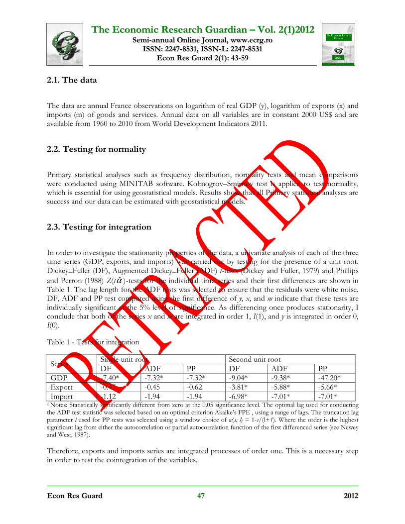
and Perron (1988) Z(tα̂ )-tests for the individual time series and their first differences are shown in Table 1. The lag length for the ADF tests was selected to ensure that the residuals were white noise. DF, ADF and PP test computed using the first difference of y, x, and m indicate that these tests are individually significant at the 5% level of significance. As differencing once produces stationarity, I conclude that both of the series x and m are integrated in order 1, I(1), and y is integrated in order 0, I(0).

Table 1 - Tests for integration

Series Single unit root Second unit root DF ADF PP DF ADF PP

GDP -7.40* -7.32* -7.32* -9.04* -9.38* -47.20* Export -0.47 -0.45 -0.62 -3.81* -5.88* -5.66* Import -1.12 -1.94 -1.94 -6.98* -7.01* -7.01*

a Notes: Statistically significantly different from zero at the 0.05 significance level. The optimal lag used for conducting the ADF test statistic was selected based on an optimal criterion Akaike’s FPE , using a range of lags. The truncation lag parameter l used for PP tests was selected using a window choice of w(s, l) = 1-s/(l+1). Where the order is the highest significant lag from either the autocorrelation or partial autocorrelation function of the first differenced series (see Newey and West, 1987).

Therefore, exports and imports series are integrated processes of order one. This is a necessary step in order to test the cointegration of the variables.




2.4. Testing for cointegration

Using the concept of a stochastic trend, we may ask whether our series are driven by common trends (Stock and Watson, 1988) or, equivalently, whether they are cointegrated (Engle and Granger, 1987). A hypothesis on investigating cointegrating relationship and certain linear restrictions were tested with using ARDL which proposed by Pesaran and Shin (1995), Pesaran and Pesaran (1997), and Pesaran et al. (2001). Result of ARDL test confirms that there is not a significant relationship between our variables in long run. Therefore we can only test Granger causality in short run with VAR method.

2.5. Investigating Granger causality

In this section we will first review the basic idea of Granger causality formulated for analyzing linear systems and then propose a generalization of Engle Granger’s idea to attractors reconstructed with geostatistical models coordinates.

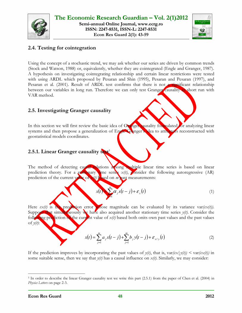
2.5.1. Linear Granger causality test5

The method of detecting causal relations among multiple linear time series is based on linear prediction theory. For a stationary time series x(t), consider the following autoregressive (AR) prediction of the current value of x(t) based on m past measurements:

( ) ( ) ( )∑=

+−=m

j

xjtjtxtx

1

εα (1)

Here εx(t) is the prediction error whose magnitude can be evaluated by its variance var(εx(t)). Suppose that simultaneously we have also acquired another stationary time series y(t). Consider the following prediction of the current value of x(t) based both onits own past values and the past values of y(t):

( ) ( ) ( ) ( )∑∑==

+−+−=m

j

yxj

m

j

jtjtybjtxatx

1

/

1

ε (2)

If the prediction improves by incorporating the past values of y(t), that is, var(εx|y(t)) < var(εx(t)) in some suitable sense, then we say that y(t) has a causal influence on x(t). Similarly, we may consider:

5 In order to describe the linear Granger causality test we write this part (2.5.1) from the paper of Chen et al. (2004) in Physics Letters on page 2-3.




( ) ( ) ( )∑=

+−=m

j

yjtjtyBty

1

ε (3)

( ) ( ) ( ) ( )tjtydjtxctyxy

m

j

j

m

j

j /

11

ε∑∑==

+−+−= (4)

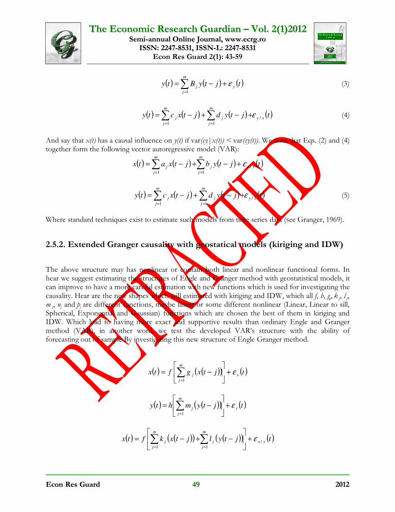
And say that x(t) has a causal influence on y(t) if var(εy|x(t)) < var(εy(t)). We note that Eqs. (2) and (4) together form the following vector autoregressive model (VAR):

( ) ( ) ( ) ( )∑∑==

+−+−=m

j

yxj

m

j

jtjtybjtxatx

1

/

1

ε

( ) ( ) ( ) ( )tjtydjtxctyxy

m

j

j

m

j

j /

11

ε∑∑==

+−+−= (5)

Where standard techniques exist to estimate such models from time series data (see Granger, 1969).

2.5.2. Extended Granger causality with geostatical models (kiriging and IDW)

The above structure may has nonlinear or contain both linear and nonlinear functional forms. In hear we suggest estimating the structures of Engle and Granger method with geostatistical models, it can improve to have a more careful estimation with new functions which is used for investigating the causality. Hear are the new shapes which will estimated with kiriging and IDW, which all f, h, gj, k j, l j, m j, nj and pj are different functions, maybe linear or some different nonlinear (Linear, Linear to sill, Spherical, Exponential and Gaussian) functions which are chosen the best of them in kiriging and IDW. Which lead to having more exact and supportive results than ordinary Engle and Granger method (VAR), in another word, we test the developed VAR’s structure with the ability of forecasting out of sample By investigating this new structure of Engle Granger method.

( ) ( )( ) ( )tjtxgftx x

m

j

j ε+

−= ∑

=1

( ) ( )( ) ( )tjtymhty y

m

j

j ε+

−= ∑

=1

( ) ( )( ) ( )( ) ( )tjtyljtxkftx yx

m

j

j

m

j

j /

11

ε+

−+−= ∑∑

==




( ) ( )( ) ( )( ) ( )tjtypjtxnhty xy

m

j

j

m

j

j /

11

ε+

−+−= ∑∑

==

(6)

2.6. Geostatistical analysis

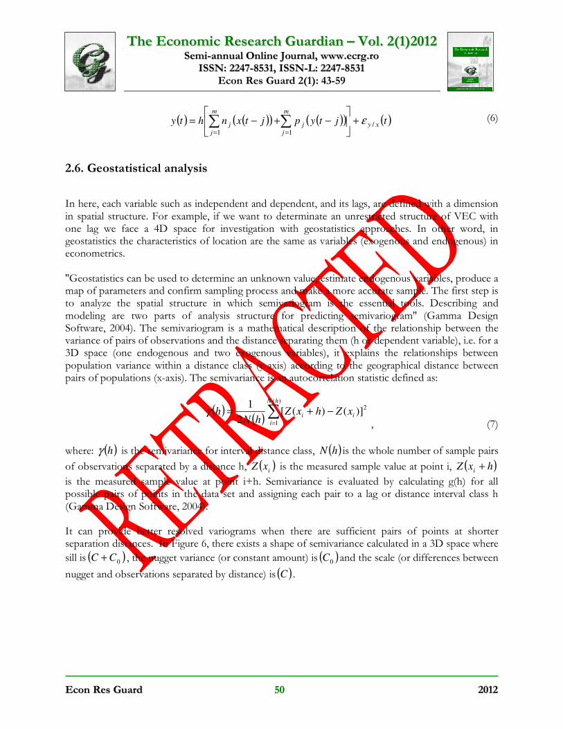
In here, each variable such as independent and dependent, and its lags, are defined with a dimension in spatial structure. For example, if we want to determinate an unrestricted structure of VEC with one lag we face a 4D space for investigation with geostatistics approaches. In other word, in geostatistics the characteristics of location are the same as variables (exogenous and endogenous) in econometrics. ''Geostatistics can be used to determine an unknown value, estimate endogenous variables, produce a map of parameters and confirm sampling process and make a more accurate sample. The first step is to analyze the spatial structure in which semivariogram is the essential tools. Describing and modeling are two parts of analysis structure for predicting semivariogram'' (Gamma Design Software, 2004). The semivariogram is a mathematical description of the relationship between the variance of pairs of observations and the distance separating them (h or dependent variable), i.e. for a 3D space (one endogenous and two exogenous variables), it explains the relationships between population variance within a distance class (y-axis) according to the geographical distance between pairs of populations (x-axis). The semivariance is an autocorrelation statistic defined as:

( )( )

2)(

1

)]()([2

1i

hN

i

i xZhxZhN

h −+= ∑=

γ , (7)

where: ( )hγ is the semivariance for interval distance class, ( )hN is the whole number of sample pairs

of observations separated by a distance h, ( )i

xZ is the measured sample value at point i, ( )hxZi

+

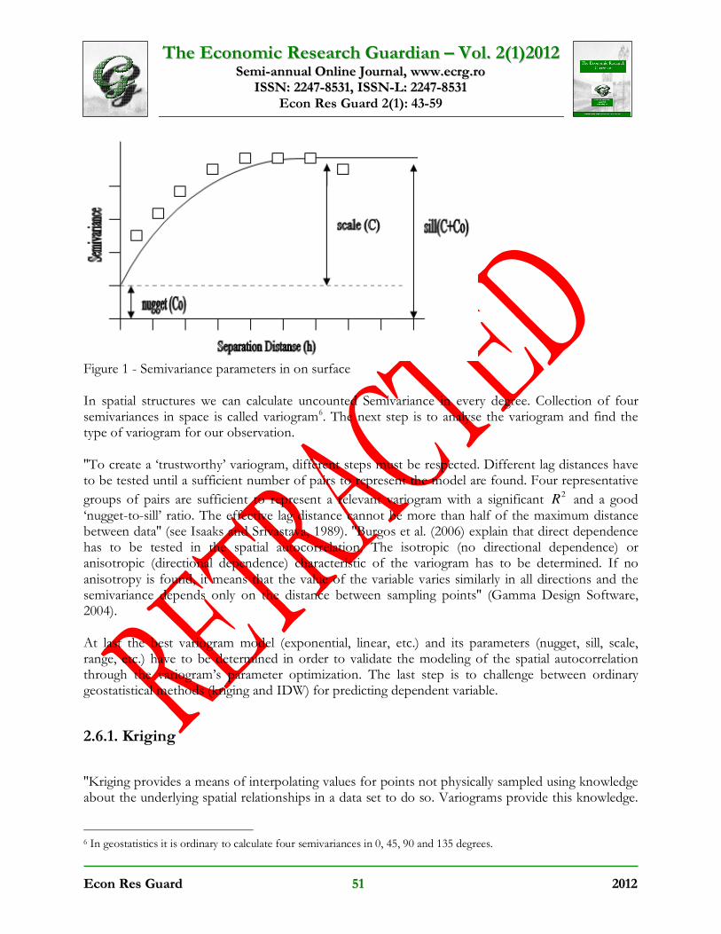
is the measured sample value at point i+h. Semivariance is evaluated by calculating g(h) for all possible pairs of points in the data set and assigning each pair to a lag or distance interval class h (Gamma Design Software, 2004). It can provide better resolved variograms when there are sufficient pairs of points at shorter separation distances. In Figure 6, there exists a shape of semivariance calculated in a 3D space where

sill is ( )0

CC + , the nugget variance (or constant amount) is ( )0

C and the scale (or differences between

nugget and observations separated by distance) is ( )C .




Figure 1 - Semivariance parameters in on surface In spatial structures we can calculate uncounted Semivariance in every degree. Collection of four semivariances in space is called variogram6. The next step is to analyse the variogram and find the type of variogram for our observation. ''To create a ‘trustworthy’ variogram, different steps must be respected. Different lag distances have to be tested until a sufficient number of pairs to represent the model are found. Four representative

groups of pairs are sufficient to represent a relevant variogram with a significant 2R and a good

‘nugget-to-sill’ ratio. The effective lag distance cannot be more than half of the maximum distance between data'' (see Isaaks and Srivastava, 1989). ''Burgos et al. (2006) explain that direct dependence has to be tested in the spatial autocorrelation. The isotropic (no directional dependence) or anisotropic (directional dependence) characteristic of the variogram has to be determined. If no anisotropy is found, it means that the value of the variable varies similarly in all directions and the semivariance depends only on the distance between sampling points'' (Gamma Design Software, 2004). At last the best variogram model (exponential, linear, etc.) and its parameters (nugget, sill, scale, range, etc.) have to be determined in order to validate the modeling of the spatial autocorrelation through the variogram’s parameter optimization. The last step is to challenge between ordinary geostatistical methods (kriging and IDW) for predicting dependent variable.

2.6.1. Kriging

''Kriging provides a means of interpolating values for points not physically sampled using knowledge about the underlying spatial relationships in a data set to do so. Variograms provide this knowledge.

6 In geostatistics it is ordinary to calculate four semivariances in 0, 45, 90 and 135 degrees.




Kriging is based on regionalized variable theory and is superior to other means of interpolation because it provides an optimal interpolation estimate for a given coordinate location, as well as a variance estimate for the interpolation value'' (Gamma Design Software, 2004). In kriging, before determining the models, it is necessary to evaluate variogram to realize whether it is isotropic or anisotropic. ''The best way to evaluate anisotropy is to view the anisotropic semivariance surface (Semivariance Map), if anisotropic semivariance surface was symmetrical variogram would be isotropic, and if it was asymmetrical variogram would be anisotropic. The differences between variogram types, isotropic and anisotropics, lead to calculate same or various weights in space for kriging model. After the variogram estimation, the interpolation between the measurement points was carried out. To do this, ordinary kriging method was used to interpolate a great number of local scour maps of exogenous and endogenous variables7. Geostatistical and spatial correlation analyses of basic infiltration rate redistribution were performed with version 5.1 of +

GS software'' (Gamma Design Software, 2004).

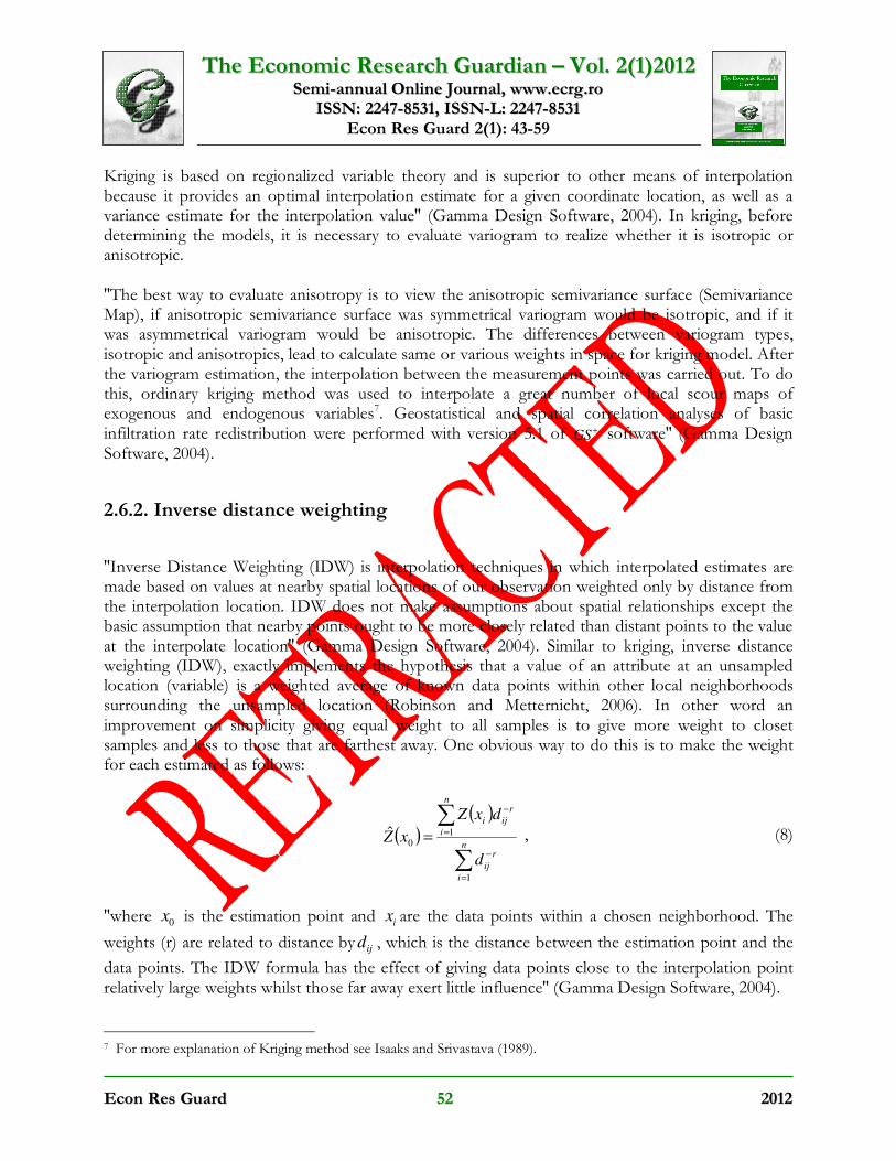
2.6.2. Inverse distance weighting

''Inverse Distance Weighting (IDW) is interpolation techniques in which interpolated estimates are made based on values at nearby spatial locations of our observation weighted only by distance from the interpolation location. IDW does not make assumptions about spatial relationships except the basic assumption that nearby points ought to be more closely related than distant points to the value at the interpolate location'' (Gamma Design Software, 2004). Similar to kriging, inverse distance weighting (IDW), exactly implements the hypothesis that a value of an attribute at an unsampled location (variable) is a weighted average of known data points within other local neighborhoods surrounding the unsampled location (Robinson and Metternicht, 2006). In other word an improvement on simplicity giving equal weight to all samples is to give more weight to closet samples and less to those that are farthest away. One obvious way to do this is to make the weight for each estimated as follows:

( )( )

∑

∑

=

−

=

−

=n

i

r

ij

n

i

r

iji

d

dxZ

xZ

1

1

0ˆ , (8)

''where 0

x is the estimation point and i

x are the data points within a chosen neighborhood. The

weights (r) are related to distance by ijd , which is the distance between the estimation point and the

data points. The IDW formula has the effect of giving data points close to the interpolation point relatively large weights whilst those far away exert little influence'' (Gamma Design Software, 2004).

7 For more explanation of Kriging method see Isaaks and Srivastava (1989).




3. Results

In this section we will first attention to results of the basic Granger causality formulated for analyzing linear systems and then probe a generalization of Engle and Granger’s idea to attractors reconstructed with geostatistical analyzing coordinates.

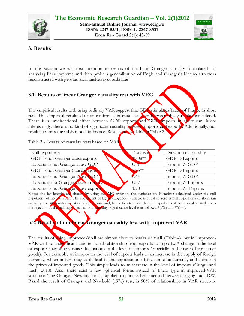
3.1. Results of linear Granger causality test with VEC

The empirical results with using ordinary VAR suggest that GDP stimulates Trade of France in short run. The empirical results do not confirm a bilateral causality between the variables considered. There is a unidirectional effect between GDP_exports and GDP_imports in short run. More interestingly, there is no kind of significant causality between imports and exports. Additionally, our result supports the GLE model in France. Results are available in Table 2.

Table 2 - Results of causality tests based on VAR

Notes: the lag lengths are chosen by using the AIC criterion; the statistics are F-statistic calculated under the null hypothesis of no causation. The coefficient of lag of exogenous variable is equal to zero is null hypothesis of short ran

causality test. ⇏ denotes statistical insignificance and, hence fails to reject the null hypothesis of non-causality. ⇒ denotes the rejection of the null hypothesis of non-causality. Significance level is as follows: *(5%) and **(1%).

3.2. Results of nonlinear Granger causality test with Improved-VAR

The results of using Improved-VAR are almost close to results of VAR (Table 4), but in Improved-VAR we find a significant unidirectional relationship from exports to imports. A change in the level of exports may simply cause fluctuations in the level of imports (especially in the case of consumer goods). For example, an increase in the level of exports leads to an increase in the supply of foreign currency, which in turn may easily lead to the appreciation of the domestic currency and a drop in the prices of imported goods. This simply leads to an increase in the level of imports (Gurgul and Lach, 2010). Also, there exist a few Spherical forms instead of linear type in improved-VAR structure. The Granger-Newbold test is applied to choose best method between kriging and IDW. Based the result of Granger and Newbold (1976) test, in 90% of relationships in VAR structure

Null hypotheses F-statistic Direction of causality

GDP is not Granger cause exports 18.08** GDP ⇒ Exports

Exports is not Granger cause GDP 0.51 Exports ⇏ GDP

GDP is not Granger Cause imports 7.95** GDP ⇒ Imports

Imports is not Granger cause GDP 0.64 Imports ⇏ GDP

Exports is not Granger Cause imports 0.57 Exports ⇏ Imports

Imports is not Granger cause exports 1.78 Imports ⇏ Exports




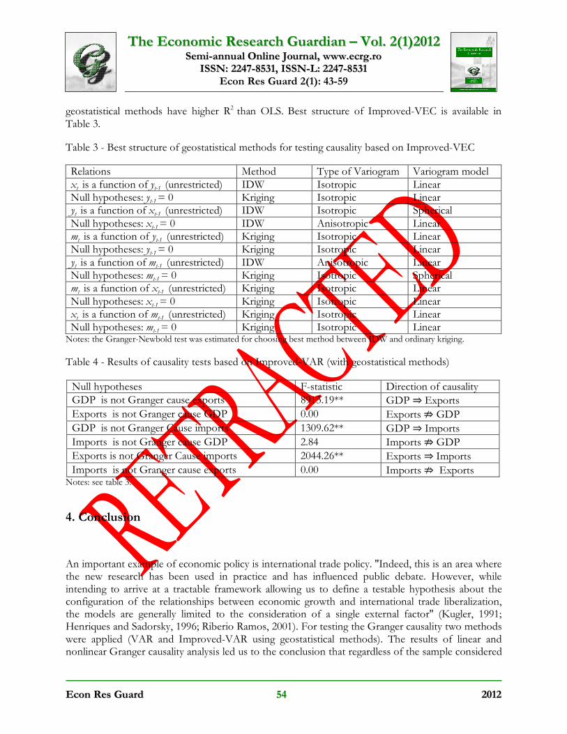
geostatistical methods have higher R2 than OLS. Best structure of Improved-VEC is available in Table 3.

Table 3 - Best structure of geostatistical methods for testing causality based on Improved-VEC

Relations Method Type of Variogram Variogram model xt is a function of yt-1 (unrestricted) IDW Isotropic Linear Null hypotheses: yt-1 = 0 Kriging Isotropic Linear yt is a function of xt-1 (unrestricted) IDW Isotropic Spherical Null hypotheses: xt-1 = 0 IDW Anisotropic Linear mt is a function of yt-1 (unrestricted) Kriging Isotropic Linear Null hypotheses: yt-1 = 0 Kriging Isotropic Linear yt is a function of mt-1 (unrestricted) IDW Anisotropic Linear Null hypotheses: mt-1 = 0 Kriging Isotropic Spherical mt is a function of xt-1 (unrestricted) Kriging Isotropic Linear Null hypotheses: xt-1 = 0 Kriging Isotropic Linear xt is a function of mt-1 (unrestricted) Kriging Isotropic Linear Null hypotheses: mt-1 = 0 Kriging Isotropic Linear Notes: the Granger-Newbold test was estimated for choosing best method between IDW and ordinary kriging.

Table 4 - Results of causality tests based on Improved-VAR (with geostatistical methods)

Notes: see table 3.

4. Conclusion

An important example of economic policy is international trade policy. ''Indeed, this is an area where the new research has been used in practice and has influenced public debate. However, while intending to arrive at a tractable framework allowing us to define a testable hypothesis about the configuration of the relationships between economic growth and international trade liberalization, the models are generally limited to the consideration of a single external factor'' (Kugler, 1991; Henriques and Sadorsky, 1996; Riberio Ramos, 2001). For testing the Granger causality two methods were applied (VAR and Improved-VAR using geostatistical methods). The results of linear and nonlinear Granger causality analysis led us to the conclusion that regardless of the sample considered

Null hypotheses F-statistic Direction of causality

GDP is not Granger cause exports 8913.19** GDP ⇒ Exports

Exports is not Granger cause GDP 0.00 Exports ⇏ GDP

GDP is not Granger Cause imports 1309.62** GDP ⇒ Imports

Imports is not Granger cause GDP 2.84 Imports ⇏ GDP

Exports is not Granger Cause imports 2044.26** Exports ⇒ Imports

Imports is not Granger cause exports 0.00 Imports ⇏ Exports




there was unidirectional relationship from GDP to trade in France. Results from these two methods were near; both show the existence of short run unidirectional causality from GDP to exports and imports. On the other hand, strong support for the existence of unidirectional relationship from exports to imports was found based on Improved-VAR. Also, in Improved-VAR there exist a few nonlinear forms instead of linear in Engle and Granger structures. In general, one may wonder whether these results provide a solid basis to claim that the good shape of the France economy during the financial crisis of 2008 was a consequence of high domestic demand rather than the impact of foreign trade in short run.

Acknowledgements

We are grateful to the anonymous referee and the editor for their useful comments. We assume all responsibility for any errors remaining in this article.

References

Ahmad J, Kwan AC (1991). Causality between exports and economic growth: empirical evidence from Africa. Economics Letters. 37: 243-248. Awokuse TO (2007). Causality between exports, imports, and economic growth: Evidence from transition economies. Economics Letters. 94 (3): 389-395. Balassa B (1978). Exports and economic growth: further evidence. Journal of Development Economics. 5: 181-189. Balassa B (1985). Exports, policy choices, and economic growth in developing countries after the 1973 oil shock. Journal of Development Economics. 18: 23-35. Bhagwati JN (1988). Protectionism. MIT Press. Cambridge. Massachusetts. Bishop TFA, McBratney AB (2001). A comparison of prediction methods for the creation of field-extent soil property maps. Geoderma. 103: 149-160. Buffie E (1992). On the condition for export-led growth. Canadian Journal of Economics. 25: 211-225. Burgos P, Madejon E, Perez-de-Mora A, Cabrera F (2006). Spatial variability of the chemical characteristics of a trace-element-contaminated soil before and after remediation. Geoderma. 130(1-2): 157-175. Cetintas H, Barisik S (2009). Export, Import and Economic Growth: The Case of Transition Economies. Transition Studies Review. 15 (4): 636-649.




Chen Y, Rangarajan G, Feng J, Ding M (2004). Analyzing multiple nonlinear time series with extended Granger causality. Physics Letters. 324: 26-35. Chow PCY (1987). Causality between export growth and industrial performance: evidence from NICs. Journal of Development Economics. 26(1): 55-63. Coe TD (1995). Helpman E. International R&D spillovers. European Economic Review. 39: 859-887. Cressie N (1985). Fitting variogram models by weighted least squares. Mathematical Geology. 17: 563-586. Cressie N (1991). Statistics for Spatial Data. John Wiley. USA: New York. Darrat AF (1986). Trade and development: the Asian experience. Cato Journal. 6: 695-699. David M (1977). Geostatistical Ore Reserve Estimation. Elsevier, Scientific Publishing. The Netherlands: Amsterdam. Dickey D, Fuller W (1979). Distribution of the estimators for autoregressive time series with a unit root. Journal of American Statisic Association. 74: 427-431.

Diks C, Panchenko V (2006). A new statistic and practical guidelines for nonparametric Granger causality testing. Journal of Economic Dynamics & Control. 30: 1647-1669. Dodaro S (1993). Exports and growth: a reconsideration of causality. Journal of Developing Areas. 27: 227-244. Doyle E (1998). Export output causality: the Irish case 1953–93. Atlantic Economic Journal. 26(2): 147-161. Edwards S (1998). Openness, productivity and growth: what do we really know? Economic Journal. 108: 383-398. Engle RF, Granger CW (1987). Co-integration and error correction: representation, estimation and testing. Econometrica. 55: 251-276. Feder G (1982). On exports and economic growth. Journal of Development Economics. 12: 59-73. Gama Design Software (2004). GSp Version 5.1. Geostatistics for the Environmental Sciences, User’s guide. Gama Design Software, LLC pp. 160. Gamal El-Din A, Smith DW (2002). A neural network model to predict the wastewater inflow incorporating rainfall events. Water Research. 36: 1115-1126.




Giles DEA, Giles JA, McCann E (1992). Causality, unit roots, and export led growth: the New Zealand experience. Journal of International Trade and Economic Development. 1: 195-218. Gilles JA, Williams CL (1999). Export led growth: a survey of the empirical literature and some noncausality results. Econometric Working Paper EWP9901, Department of Economics, University of Victoria. Granger CWJ (1969). Investigating causal relations by econometric models and crossspectral models. Econometrica 37: 424-438. Granger CWJ, Newbold P (1976). The use of R2 to determine the appropriate transformation of regression variables. Journal of Econometrics. 4: 205-210. Grossman G, Helpman E (1991). Innovation and Growth in the Global Economy. Cambridge, MA: MIT Press. Gurgul H, Lach L (2010). International trade and economic growth in the Polish economy. Operations

Research and Decisions No. 3-4. Findlay R (1984). Growth and Development in Trade Models. in Handbook of International Economics, vol. 1, (eds). Jones R and Kenen P, Amsterdam: North-Holland. Helpman E, Krugman P (1985). Market Structure and Foreign Trade. Cambridge, MA: MIT Press. Henriques I, Sadorsky P (1996). Export-Led Growth or Growth-Driven Exports? The Canadian Case. Canadian Journal of Economics. 25: 211-225. Hill T, Marquez L, O'Connor M, Remus W (1994). Artificial Neural Network Models for Forecasting and Decision Making. International Journal of Forecasting. 10: 5-15. Hsiao MCW (1987). Tests of causality and exogenity between exports and economic growth: the case of the Asian NIC’s. Journal of Economic Development. 12(2): 143-159. Isaaks EH, Srivstava RM (1989). Applied Goestatistics. New York Oxford University Press. pp. 257-259. Jiang LF, Wen L (2009). An Econometric Model of The Relationship Between Foreign Trade and Economic Growth in China. Second International Conference on Information and Computing Science. Jung WS, Marshall PJ (1985). Exports, growth and causality in developing countries. Journal of Development Economics. 1985, 18(1): 1-12. Krige DG (1981). Lognormal-de Wijsian geostatistics for ore evaluation. South African Institute of Mining and Metallurgy Monograph Series. Geostatistics I. South Africa Institute of Mining and Metallurgy, South Africa: Johannesburg.




Krugman PR (1984). Import protection as export promotion. In: Kierzkowski, H. (Ed.), Monopolistic Competition in International Trade. Oxford University Press, Oxford. Kugler P (1991). Growth, Exports and Cointegration: An Empirical Investigation, Weltwirtschaftliches Archive. pp. 73-82. Lawrence RZ, Weinstein DE (1999). Trade and growth: import-led or export-led? Evidense from Japan and Korea. NBER Working Paper. 7264. Mabit L, Bernard C (2007). Assessment of spatial distribution of fallout radionuclides through geostatistics concept. Journal of Environmental Radioactivity. 97: 206-219. Marin D (1992). Is the export-led growth hypothesis valid for industrialized countries? Review of Economics and Statistics. 74: 678-688. Mazumdar J (2000). Imported machinery and growth in LDCs. Journal of Development Economics. 65: 209-224. Michaely M (1977). Exports and growth: an empirical investigation. Journal of Development Economics. 40: 149-153. Newey W, West K (1987). A simple, positive semi-definite, heteroscedasticity and autocorrelation consistent covariance matrix. Econometrica. 55: 703-708. Oxley L (1993). Cointegration, causality and export-led growth in Portugal, 1865_1985. Economics Letters. 43: 163-166. Pesaran MH, Pesaran B (1997). Working with Microfit 4.0. Camfit Data Ltd, Cambridge. Pesaran MH, Shin Y (1995). An autoregressive distributed lag modeling approach to cointegration analysis. DAE Working Paper No. 9514, Department of Applied Economics, University of Cambridge, forthcoming in S. Strom, A. Holly and P. Diamond (eds) centennial volume of Ranger Frisch. Pesaran MH, Shin Y, Smith RJ (2001). Bounds testing approaches to the analysis of level relationships. Journal of Applied Econometrics. 16: 289-326. Phillips P, Perron P (1988). Testing for a unit root in time series regression. Biometrika. 75: 335-346. Ram R (1987). Exports and economic growth in developing countries: evidence from time series and cross–section data. Economic Development and Cultural Change. 36: 51-72. Ribeiro Ramos FF (2001). Exports, imports, and economic growth in Portugal: evidence from causality and cointegration analysis. Economic Modelling. 18: 613-623.




Rivera-Batiz L, Romer P (1991). Economic integration and endogenous growth. Journal of Economics. 106: 531-556. Robinson TP, Metternicht G (2006). Testing the performance of spatial interpolation techniques for mapping soil properties. Computer and Electronics in Agriculture. 50: 97-108. Romer P (1990). Endogenous technological change. Journal of Politic Economics. 98: 71-102. Segerstrom P, Anant T, Dinopoulos E (1990). A Shumpeterian model of the product life cycle. American Economic Review. 80: 1077-1091. Shan J, Sun F (1998). On the export led growth hypothesis for the little dragons: an empirical reinvestigation. Atlantic Economic Journal. 26: 353-371. Sims CA (1972) Money, income, and causality.The American Economic Review. 62: 540-552. Stock J, Watson M (1988). Testing for common trends. Journal of America Statistic Association. 83: 1097-1107. Thornton J (1996). Cointegration, causality and export-led growth in Mexico. Economics Letters. 50: 413-416. Tyler WG (1981). Growth and export expansion in developing countries: some empirical evidence. Journal of Development Economics. 9: 121-130. Van Kuilemberg J, De Gruitjer J, Marsman B, Bouma J (1982). Accuracy of spatial interpolation between point data on soil moisture supply capacity, compared with estimates from mapping units. Geoderma. 27, 311-325. Venables A (1996). Equilibrium locations of vertically linked industries. International Economic Review. 37: 341-359. Vernon R (1996). International investment and international trade in the product cycle. Journal of Econometric Society Monograph. 80: 190-207.

Voltz M, Webster R (1990). A comparison of kriging, cubic splines and classification for predicting soil properties from sample information. Journal of Soil Science. 41: 473-490. Wörz J (2005). Skill Intensity in Foreign Trade and Economic Growth. Springer Netherlands, Volume 32, Number:1. Xu Z (1996). On the causality between export growth and GDP growth: an empirical evidence. Review of International Economics. 4(6): 172-184.

granger causality between exports, imports and …1)6y3.pdfcausal links between foreign trade and...

Documents