gradient,divergence,curl...
TRANSCRIPT
Gradient, Divergence, Curl
and Related Formulae
The gradient, the divergence, and the curl are first-order differential operators acting on
fields. The easiest way to describe them is via a vector nabla whose components are partial
derivatives WRT Cartesian coordinates (x, y, z):
∇ = x∂
∂x+ y
∂
∂y+ z
∂
∂z. (1)
When acting on a field, ∇ transforms like a true vector under rigid rotations of the coordinate
system:
x
y
z
→
x′
y′
z′
=
Tx′x Tx′y Tx′z
Ty′x Ty′y Ty′z
Tz′x Tz′y Tz′z
x
y
z
,
∇′ = x′∂
∂x′+ y′ ∂
∂y′+ z′
∂
∂z′= ∇.
(2)
Note: eqs. (1) and (2) work only in Cartesian coordinates (3 straight axes ⊥ to each other). In
curvilinear coordinates, formulae for the ∇ are more complicated.
Acting with the ∇ operator on a scalar field S(x, y, z) produces a vector field
∇S =∂S
∂xx +
∂S
∂yy +
∂S
∂zz = gradS(x, y, z) (3)
called the gradient of S. Physically, the gradient measures how much S is changing with the
location; it points in the direction of steepest increase of S while its magnitude is the rate of
that increase. At the local maxima, local minima, or other stationary points of S, the gradient
vanishes.
Leibniz rule for the gradient of a product of two scalar fields S1(x, y, z) and S2(x, y, z):
∇(
S1S2) = S1∇S2 + S2∇S1. (4)
Chain Rule for the gradient of a function of another function of the 3 coordinates:
If P (x, y, z) = f(
S(x, y, z))
, then ∇P =dP
dS∇S. (5)
1
As an example, let’s apply this rule to a spherically symmetric field
P (x, y, z) = P (r only), r = |r| =√
x2 + y2 + z2. (6)
By the chain rule, the gradient of any such field is
∇P (r) =dP
dr∇r =
dP
drr (7)
where the second equality follows from the gradient of the radius r being the unit vector r in
the radial direction. This should be obvious from the physical meaning of the gradient, but
let’s prove this mathematically. Let’s start with the gradient of r2 = x2 + y2 + z2:
∇(r2) =
(
x∂
∂x+ y
∂
∂y+ z
∂
∂z
)
(
x2 + y2 + z2)
= 2x x+ 2y y + 2z z = 2r. (8)
At the same time, by the chain rule,
∇(r2) =dr2
dr∇r = 2r∇r, (9)
hence
∇r =1
2r∇(r2) =
1
2r(2r) = r, (10)
quod erat demonstrandum.
As an example of eq. (7), the gradient of any power of the radius is
∇(
rn)
= nrn−1 r. (11)
2
The Divergence of a vector field V(x, y, z) is a scalar field divV(x, y, z) which measures how
much V spreads out at each point (x, y, z) (or for a negative divergence, how much V converges
to the point (x, y, z)). Algebraically, the divergence is the scalar product (dot product) of the
∇ operator and the vector field on which it acts:
divV(x, y, z) = ∇ ·V =∂
∂xVx +
∂
∂yVy +
∂
∂zVz . (12)
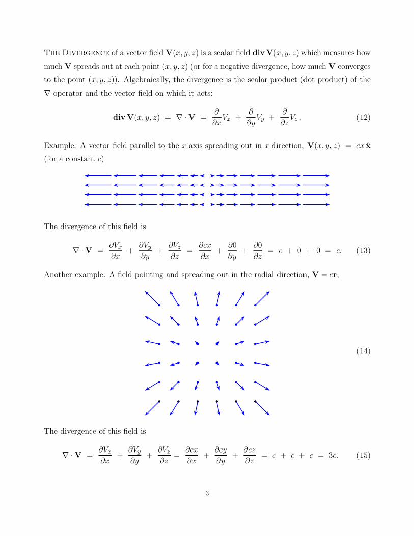
Example: A vector field parallel to the x axis spreading out in x direction, V(x, y, z) = cx x
(for a constant c)
The divergence of this field is
∇ ·V =∂Vx∂x
+∂Vy∂y
+∂Vz∂z
=∂cx
∂x+
∂0
∂y+
∂0
∂z= c + 0 + 0 = c. (13)
Another example: A field pointing and spreading out in the radial direction, V = cr,
(14)
The divergence of this field is
∇ ·V =∂Vx∂x
+∂Vy∂y
+∂Vz∂z
=∂cx
∂x+
∂cy
∂y+
∂cz
∂z= c + c + c = 3c. (15)
3
Similar to the Leibniz rule for the gradient, there is a Leibniz rule for the divergence of a
product of a scalar field S(x, y, z) and a vector field V(x, y, z):
∇ ·(
SV)
=(
∇S)
·V + S(
∇ ·V)
. (16)
This rule is particularly useful for calculating divergences of spherically symmetric radial fields
V(x, y, z) = V (r only) r =V (r)
rr (17)
Indeed, by the Leibniz rule (16),
∇ ·(
V =V (r)
rr
)
=
(
∇(
V (r)
r
))
· r +V (r)
r
(
∇ · r)
(18)
where in the second term on the RHS ∇ · r = 3, cf. the example (15). As to the first term on
the RHS,
∇(
V (r)
r
)
=d(V/r)
drr =
(
V ′
r− V
r2
)
r (19)
and hence(
∇(
V (r)
r
))
· r =
(
V ′
r− V
r2
)
×(
r · r = r)
=dV
dr− V
r. (20)
Plugging this formula and ∇ · r = 3 into eq. (18), we arrive at
∇ · (V = V (r) r) =dV
dr− V
r+
V
r× 3 =
dV
dr+ 2
V
r. (21)
In particular, for V (r) = krn (for a constant k),
∇ ·(
krn r)
= nkrn−1 + 2krn−1 = (n+ 2)krn−1 . (22)
Note: the Coulomb electric field of a point charge has this form for n = −2. Consequently,
for E =Q
4πǫ0
r
r2, ∇ · E =
(
(n = −2) + 2 = 0)
× Q
4πǫ0× 1
r3= 0, (23)
the Coulomb electric field seems to be divergence-less! However, this formula is valid only
outside the charge, at r 6= 0, but right on top of the charge, at r = 0, the electric field itself is
singular and its divergence is actually infinite. As we shall see later in class,
for E =Q
4πǫ0
r
r2, ∇ · E(r) =
Q
ǫ0× δ(3)(r). (24)
4
The Curl or rotor of a vector field V(x, y, z) is another vector field curlV(x, y, z) which
measure the vorticity of the V field. Specifically, the x component of the curlV measure the
vorticity of the V field in the yz plane (and thus around the x axis), and likewise for the y and
z components.
Algebraically, curlV(x, y, z) obtains as a vector product of the ∇ and the vector field V
on which it acts:
curlV = rotV = ∇×V
=
(
x∂
∂x+ y
∂
∂y+ z
∂
∂z
)
×(
xVz + yVy + zVz
)
= det
x y z
∂∂x
∂∂y
∂∂z
Vx Vy Vz
= x
(
∂Vz∂y
− ∂Vy∂z
)
+ y
(
∂Vx∂z
− ∂Vz∂x
)
+ z
(
∂Vy∂x
− ∂Vx∂y
)
.
(25)
Example: the radially symmetric spreading out field (14) V(r) = cr has zero curl. Indeed,
the x component of the curl evaluates to
(
∇× (cr))
x=
∂(cr)z∂y
− ∂(cr)y∂z
=∂cz
∂y− ∂cy
∂z= 0 − 0 = 0, (26)
and likewise, the y component and the z component of ∇× (cr) also vanish.
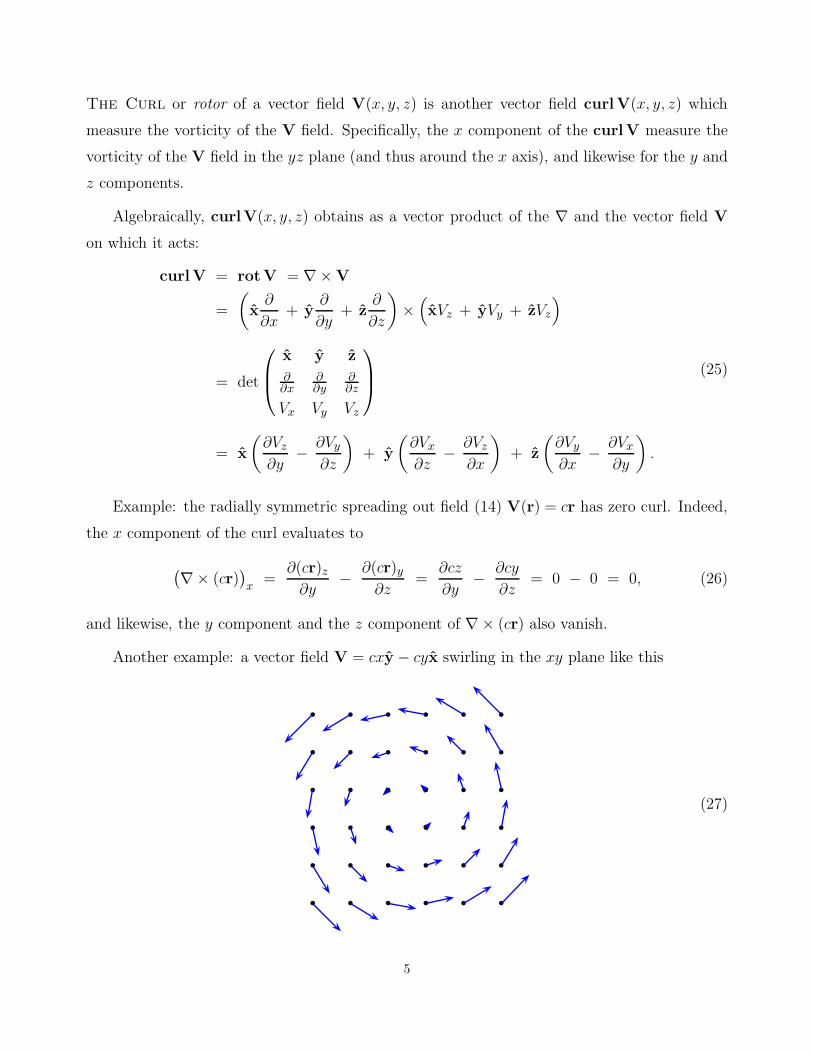
Another example: a vector field V = cxy − cyx swirling in the xy plane like this
(27)
5
has a non-trivial curl in the z direction:
(
∇× (cxy − cyx))
z=
∂(Vy = cx)
∂x− ∂(Vx = −cy)
∂y= (+c) − (−c) = 2c, (28)
while the x and y components of the curl vanish:
(
∇× (cxy − cyx))
x=
∂(Vz = 0)
∂y− ∂(Vy = +cx)
∂z= 0 − 0 = 0,
(
∇× (cxy − cyx))
y=
∂(Vx = −cy)
∂z− ∂(Vz = 0)
∂x= 0 − 0 = 0.
(29)
Leibniz rule for the curl of a product of a scalar field S(x, y, z) and a vector field V(x, y, z):
∇×(
SV)
=(
∇S)
×V + S(
∇× V)
, (30)
Using this rule, it is easy to show that any spherically symmetric radial field V(x, y, z) = V (r)r
has zero curl. Indeed,
V =V (r)
rr,
∇×V =
(
∇V
r
)
× r +V
r
(
∇× r)
where ∇× r = 0,
and ∇V
r=
d(V/r)
drr,
hence ∇×V =
(
d(V/r)
drr
)
× r + 0
=d(V/r)
dr
(
r× r = 0)
+ 0
= 0.
(31)
6
Other Leibniz rules:
(a) Divergence of a vector product of two vector fields A(x, y, z) and B(x, y, z),
∇ · (A×B) = B · (∇×A) − A · (∇×B). (32)
(b) Curl of a cross product of two vector fields,
∇× (A×B) = (B · ∇)A − (A · ∇)B + A(∇ ·B) − B(∇ ·A). (33)
(c) Gradient of a dot product of two vector fields:
∇(A ·B) = (A · ∇)B + (B · ∇)A + A× (∇×B) + B× (∇×A). (34)
In the last two formulae here (A · ∇) and (B · ∇) are not the divergences but rather the
differential operators
(A · ∇) = Ax∂
∂x+ Ay
∂
∂y+ Az
∂
∂z,
(B · ∇) = Bx∂
∂x+ By
∂
∂y+ Bz
∂
∂z,
(35)
which then act on another field. For example,
(A · ∇)S = Ax∂S
∂x+ Ay
∂S
∂y+ Az
∂S
∂z,
(A · ∇)B =
(
Ax∂Bx
∂x+ Ay
∂Bx
∂y+ Az
∂Bx
∂z
)
x +
(
Ax∂By
∂x+ Ay
∂By
∂y+ Az
∂By
∂z
)
y
+
(
Ax∂Bz
∂x+ Ay
∂Bz
∂y+ Az
∂Bz
∂z
)
z .
(36)
Second Derivatives
The gradient, the divergence, and the curl are first-order differential operators for the fields.
By acting with two such operators — one after the other — we can make interesting second-
order differential operators.
7
Thanks to ∇ × ∇ = 0, two combinations of first-order operators are identical zeros: (a)
The curl of a gradient of any scalar field vanishes identically,
for any S(x, y, z), curl(grad(S)) = ∇× (∇S) ≡ 0. (37)
(b) The divergence of a curl of any vector field vanishes identically,
for any V(x, y, z), div(curl(V)) = ∇ · (∇×V) ≡ 0. (38)
Proof: Let’s start with the curl of a gradient. For the z component of the curl, we have
(
∇× (∇S))
z=
∂
∂x(∇S)y − ∂
∂y(∇S)x =
∂
∂x
∂S
∂y− ∂
∂y
∂S
∂x= 0 (39)
because the partial derivatives WRT x, y, z can be taken in any order without changing the
result. Likewise, the x and y components of the curl of a gradient vanish for the same reason:
(
∇× (∇S))
x=
∂
∂y
∂S
∂z− ∂
∂z
∂S
∂y= 0,
(
∇× (∇S))
y=
∂
∂z
∂S
∂x− ∂
∂x
∂S
∂z= 0.
(40)
Finally, the divergence of a curl of a vector field is
∇ · (∇×V) =∂
∂x
(
∇×V)
x+
∂
∂y
(
∇×V)
y+
∂
∂z
(
∇×V)
z
=∂
∂x
(
∂Vz∂y
− ∂Vy∂z
)
+∂
∂y
(
∂Vx∂z
− ∂Vz∂x
)
+∂
∂z
(
∂Vy∂x
− ∂Vx∂y
)
〈〈 regrouping terms 〉〉
=
(
∂
∂x
∂Vz∂y
− ∂
∂y
∂Vz∂x
)
+
(
∂
∂y
∂Vx∂z
− ∂
∂z
∂Vx∂y
)
+
(
∂
∂z
∂Vy∂x
− ∂
∂x
∂Vy∂z
)
= 0 + 0 + 0 = 0.(41)
Quod erat demonstrandum.
8
Now let’s turn to the non-vanishing combinations of the derivative operators. Consider the
divergence of a gradient of a scalar field:
div(gradS) = ∇ · (∇S) =∂
∂x
∂S
∂x+
∂
∂y
∂S
∂y+
∂
∂z
∂S
∂z=
(
∂2
∂x2+
∂2
∂y2+
∂2
∂z2
)
S. (42)
The second-order differential operator inside the () on the RHS is called the Laplace operator
or simply the Laplacian; it is usually denote by the triangle ,
=∂2
∂x2+
∂2
∂y2+
∂2
∂z2. (43)
Algebraically, the Laplacian is the scalar square of the ∇ vector,
= ∇2 = ∇ · ∇ =∂
∂x
∂
∂x+
∂
∂y
∂
∂y+
∂
∂z
∂
∂z. (44)
Under rigid rotations of the Cartesian coordinates, the Laplacian transforms like a scalar —
i.e., remains invariant:
x
y
z
→
x′
y′
z′
=
Tx′x Tx′y Tx′z
Ty′x Ty′y Ty′z
Tz′x Tz′y Tz′z
x
y
z
,
′ =∂2
∂x′2+
∂2
∂y′2+
∂2
∂z′2= .
(45)
Hence, the Laplacian operator acting on a scalar field as in eq. (42) produces a scalar field.
We may also act with the Laplacian operator (43) on a vector field V(x, y, z) — by acting
on each component Vx, Vy, Vz separately — and produce a vector field
V =
(
∂2Vx∂x2
+∂2Vx∂y2
+∂2Vx∂z2
)
x +
(
∂2Vy∂x2
+∂2Vy∂y2
+∂2Vy∂z2
)
y +
(
∂2Vz∂x2
+∂2Vz∂y2
+∂2Vz∂z2
)
z.
(46)
Such Laplacian of a vector field also obtains from combining the gradient of the divergence of
that vector field with a curl of the curl,
V = ∇(∇ ·V) − ∇× (∇×V) = grad(divV) − curl(curlV). (47)
Formally, this formula obtains from the BAC − CAB rule for the double cross product of 3
9
vectors where two of them are ∇ and the third is V:
A× (B×C) = B(A ·C) − C(A ·B) = B(A ·C) − (A ·B)C,
let A = B = ∇, C = V(x, y, z),
∇× (∇×V) = ∇(∇ ·V) − (∇ · ∇)V = ∇(∇ ·V) − V.
(48)
More rigorously, we should redo the vector algebra here plugging the appropriate derivatives
for the components of the ∇ vector and making explicit use of partial derivatives commuting
with each other, but I am not doing it in these notes.
Physically, the Laplacian of the electric potential is very important in electrostatics, while
the Laplacians of the vector electric and magnetic fields are very important for the propagation
of the electromagnetic waves.
10
Integrals and Fundamental Theorems
For the functions of one variable, the derivatives and the integrals are related by the Fun-
damental theorem of calculus (also known as the Newton’s theorem:
for f ′(x) =df
dx,
B∫
A
f ′(x) dx = f(B) − f(A). (49)
There are similar theorems relating the gradients, the divergences, and the curls of fields to the
line, surface, and volume integrals.
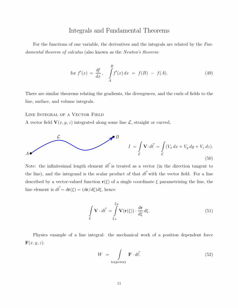
Line Integral of a Vector Field
A vector field V(x, y, z) integrated along some line L, straight or curved,
A
BL
I =
∫
L
V ·d~ℓ =
∫
L
(Vx dx + Vy dy + Vz dz).
(50)
Note: the infinitesimal length element d~ℓ is treated as a vector (in the direction tangent to
the line), and the integrand is the scalar product of that d~ℓ with the vector field. For a line
described by a vector-valued function r(ξ) of a single coordinate ξ parametrizing the line, the
line element is d~ℓ = dr(ξ) = (dr/dξ)dξ, hence
∫
L
V · d~ℓ =
ξB∫
ξA
V(r(ξ)) · drdξ
dξ. (51)
Physics example of a line integral: the mechanical work of a position dependent force
F(x, y, z).
W =
∫
trajectory
F · d~ℓ. (52)
11
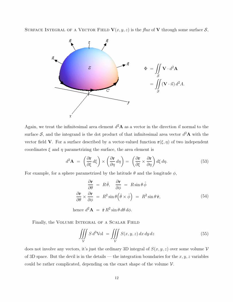
Surface Integral of a Vector Field V(x, y, z) is the flux of V through some surface S,
Φ =
∫∫
S
V · d2A
=
∫∫
S
(V · ~n) d2A.
Again, we treat the infinitesimal area element d2A as a vector in the direction ~n normal to the
surface S, and the integrand is the dot product of that infinitesimal area vector d2A with the
vector field V. For a surface described by a vector-valued function r(ξ, η) of two independent
coordinates ξ and η parametrizing the surface, the area element is
d2A =
(
∂r
∂ξdξ
)
×(
∂r
∂ηdη
)
=
(
∂r
∂ξ× ∂r
∂η
)
dξ dη. (53)
For example, for a sphere parametrized by the latitude θ and the longitude φ,
∂r
∂θ= R θ,
∂r
∂φ= R sin θ φ
∂r
∂θ× ∂r
∂φ= R2 sin θ
(
θ × φ)
= R2 sin θ r,
hence d2A = rR2 sin θ dθ dφ.
(54)
Finally, the Volume Integral of a Scalar Field
∫∫∫
V
S d3Vol =
∫∫∫
V
S(x, y, z) dx dy dz (55)
does not involve any vectors, it’s just the ordinary 3D integral of S(x, y, z) over some volume Vof 3D space. But the devil is in the details — the integration boundaries for the x, y, z variables
could be rather complicated, depending on the exact shape of the volume V.
12
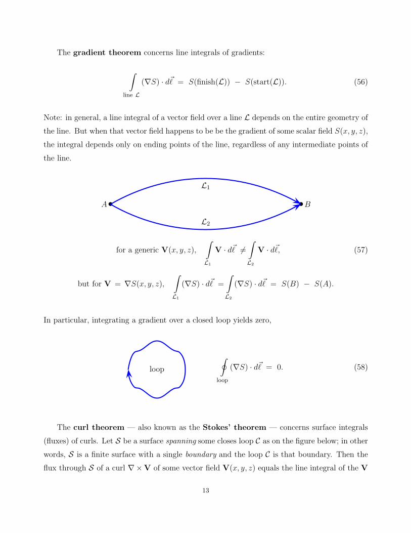
The gradient theorem concerns line integrals of gradients:
∫
line L
(∇S) · d~ℓ = S(finish(L)) − S(start(L)). (56)
Note: in general, a line integral of a vector field over a line L depends on the entire geometry of
the line. But when that vector field happens to be be the gradient of some scalar field S(x, y, z),
the integral depends only on ending points of the line, regardless of any intermediate points of
the line.
BA
L1
L2
for a generic V(x, y, z),
∫
L1
V · d~ℓ 6=∫
L2
V · d~ℓ, (57)
but for V = ∇S(x, y, z),
∫
L1
(∇S) · d~ℓ =
∫
L2
(∇S) · d~ℓ = S(B) − S(A).
In particular, integrating a gradient over a closed loop yields zero,
loop
∮
loop
(∇S) · d~ℓ = 0. (58)
The curl theorem — also known as the Stokes’ theorem — concerns surface integrals
(fluxes) of curls. Let S be a surface spanning some closes loop C as on the figure below; in other
words, S is a finite surface with a single boundary and the loop C is that boundary. Then the
flux through S of a curl ∇×V of some vector field V(x, y, z) equals the line integral of the V
13
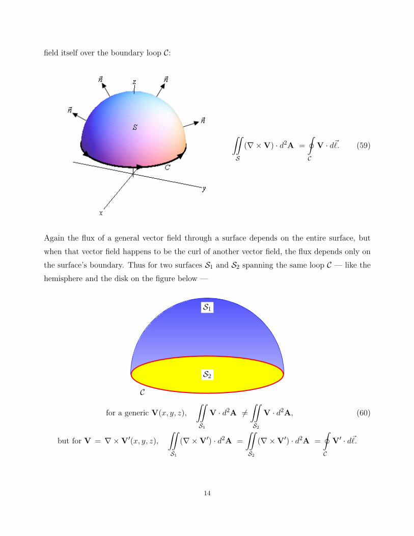
field itself over the boundary loop C:
∫∫
S
(∇×V) · d2A =
∮
C
V · d~ℓ. (59)
Again the flux of a general vector field through a surface depends on the entire surface, but
when that vector field happens to be the curl of another vector field, the flux depends only on
the surface’s boundary. Thus for two surfaces S1 and S2 spanning the same loop C — like the
hemisphere and the disk on the figure below —
S1
S2
C
for a generic V(x, y, z),
∫∫
S1
V · d2A 6=∫∫
S2
V · d2A, (60)
but for V = ∇×V′(x, y, z),
∫∫
S1
(∇×V′) · d2A =
∫∫
S2
(∇×V′) · d2A =
∮
C
V′ · d~ℓ.
14
The divergence theorem — also known as theGauss’ theorem, theGreen’s theorem,
or the Ostrogradsky’s theorem — concerns the volume integrals of the divergences of vector
fields. Let V be some finite volume of space and let S be its complete surface. Then the volume
integral over V of the divergence ∇ ·V of some vector field V(x, y, z) equals to the flux of the
V field itself through the surface S of V:
∫∫∫
V
(∇ ·V) d3Vol =
∫∫
S
V · d2A. (61)
Example: Let S be a sphere of radius R while V is the solid ball filling that sphere, and let
V(x, y, z) = f(r)r be a spherically symmetric radial vector field. As we saw earlier in these
notes in eq. (21), the divergence of such a field is
∇ ·(
f(r)r)
=df
dr+
2f
r. (62)
To integrate this divergence over the volume of the ball, we use spherical coordinates in which
the volume element is
d3Vol = r2 dr d2Ω −→ 4πr2 dr (once we integrate over the directions). (63)
Consequently, the integral of the divergence over the solid ball evaluates to
∫∫∫
ball
(∇·V) d3Vol =
R∫
0
(
df
dr+
2f
r
)
×4πr2 dr =
R∫
0
d
dr
(
4πr2×f(r))
dr = 4πR2f(R). (64)
On the other hand, the flux of the radial V field through the sphere is simply
∫∫
sphere
(
V = f(r)r)
· d2A = f(R)× Area(sphere) = f(R)× 4πR2. (65)
By inspection, this flux is equal to the volume integral (64), in perfect agreement with the
Gauss Theorem.
15
Applications to Electrostatics — the Potential
In electrostatics, the electric field lines never form any closed loops. This is a visualisation
of a stronger rule: the line integral of a static electric field over any closed loop is zero,
∀ loop C,∮
C
E · d~ℓ = 0. (66)
By the Stokes’ theorem, this means that the curl ∇× E has zero flux through any surface Sspanning any closed loop C,
∀S,∫∫
S
(∇× E) · d2A = 0. (67)
In particular, the flux through any infinitesimal square — of any orientation, and located
anywhere in space — must vanish, which means that the curl ∇ × E(x, y, z) must vanish
identically everywhere in space. Thus, the static electric field has identically zero curl,
∇×E(x, y, z) ≡ 0 ∀ x, y, z. (68)
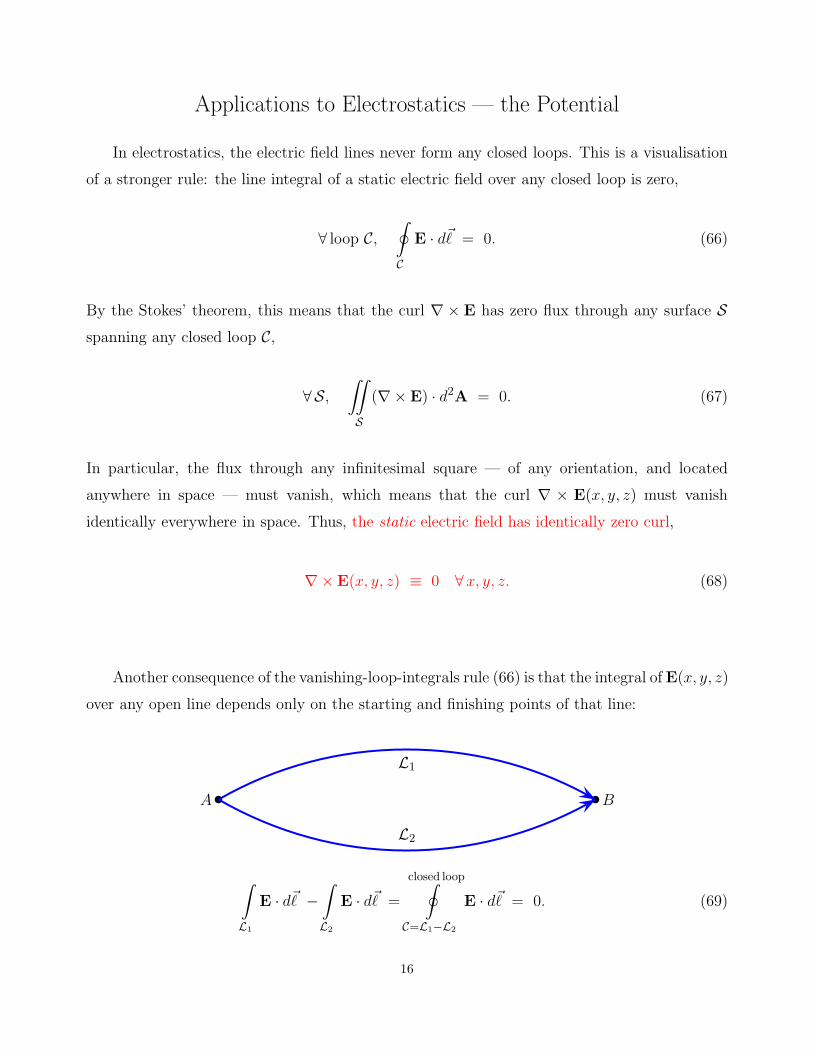
Another consequence of the vanishing-loop-integrals rule (66) is that the integral ofE(x, y, z)
over any open line depends only on the starting and finishing points of that line:
BA
L1
L2
∫
L1
E · d~ℓ −∫
L2
E · d~ℓ =
closed loop∮
C=L1−L2
E · d~ℓ = 0. (69)
16
Physically, the line integrals here are related to the work of the electrostatic force F = qE(x, y, z)
on a moving probe charge q,
W = q ×∫
trajectory
E · d~ℓ. (70)
Thus, eq. (69) means that the work of moving a probe charge from a point A to a point B
is the same regardless of a particular path the charge takes from A to B. This makes the
electrostatic force conservative. Consequently, the work of this force is related to a potential
energy U(x, y, z) — which obviously have the form
U(x, y, z) = q × V (x, y, z) (71)
for some q-independent electric potential V (x, y, z).
The potential difference between any two points A and B obtains by integrating the electric
field over any line from A to B,
V (A) − V (B) =
B∫
A
E · d~ℓ, same integral for any path from A to B. (72)
The potential itself is ambiguous — we may add a position-independent constant to the
V (x, y, z) without changing any of the differences. To remove the ambiguity, one usually picks
a reference point O where the potential is set to zero by fiat. That at any other point A,
V (A) =
O∫
A
E · d~ℓ along any path from A to O. (73)
Example: Consider the Coulomb field of a point charge at r = ~0,
E(r) =kQ
|r|2 r (74)
where k = 1/4πǫ0 (in the MKSA units). Then along any line in space,
E · d~ℓ =kQ
|r|2 r · dr =kQ
|r|2 d|r| = d
(−kQ
|r|
)
, (75)
17

and henceO∫
A
E · d~ℓ =
O∫
A
d
( −kQ
r(x, y, z)
)
=−kQ
r(O)− −kQ
r(A), (76)
regardless of the directions of the points A and O relative to the charge Q, only their distances
from the Q affect this integral. For the electric potential, this means
V (A) = +kQ
r(A)− kQ
r(O). (77)
For simplicity, let’s move the reference point O (where the potential vanishes) to the infinity,
r(O) = ∞, then the electric potential due to a point charge Q become simply
V [point charge] =Q
4πǫ0× 1
r. (78)
The superposition principle for the electric field of multiple charges carries over to the
electric potential. Thus, for a system of several point charges Qi located at points Ri, the net
electric potential is simply
V (r) =1
4πǫ0
∑
i
Qi
|r−Ri|. (79)
Note that its easier to add up the scalar potentials due to each charge than to add up the
electric field vectors. This is particularly true when the source charges are continuous rather
than point-like, and the sum (77) becomes an integral. Thus, for a volume charge density
ρ(x, y, z), the electric potential is
V (x, y, z) =1
4πǫ0
∫∫∫
ρ(x′, y′, z′)√
(x− x′)2 + (y − y′)2 + (z − z′)2dx′ dy′ dz′. (80)
This is a painful triple integral, but at least we need only one such integral rather than three
triple integrals we would need for calculating the electric field:
Ex(x, y, z) =1
4πǫ0
∫∫∫
ρ(x′, y′, z′)× (x− x′)(
(x− x′)2 + (y − y′)2 + (z − z′)2)3/2
dx′ dy′ dz′,
Ey(x, y, z) =1
4πǫ0
∫∫∫
ρ(x′, y′, z′)× (y − y′)(
(x− x′)2 + (y − y′)2 + (z − z′)2)3/2
dx′ dy′ dz′,
Ez(x, y, z) =1
4πǫ0
∫∫∫
ρ(x′, y′, z′)× (z − z′)(
(x− x′)2 + (y − y′)2 + (z − z′)2)3/2
dx′ dy′ dz′.
(81)
18
In light of the formulae like (79) and (80) for the electric potential, the obvious question is:
Given the electric potential V (x, y, z), how do we reconstruct the electric field E(x, y, z) from
this potential? The answer is very simple: take the gradient (and flip the sign),
E(x, y, z) = −∇V (x, y, z). (82)
Proof: By the gradient theorem,
B∫
A
(−∇V ) · d~ℓ = V (A) − V (B) =
B∫
A
E · d~ℓ. (83)
Both equalities here do not depend on the specific path from A to B, so let’s put point B
infinitesimally close to point A, r(B) = r(A) + dr and take the straight-line path from A to B.
In this case, the integrals simplify to integrand · dr, thus
(−(∇V )@A) · dr = (E@A) · dr. (84)
This equality must hold true for any infinitesimal dr, which requires the vector equality
−∇V = E at the same point A, for any such A. (85)
In other words, E(x, y, z) ≡ −∇V (x, y, z) as vector fields, quod erat demonstrandum.
Example: Let’s find the potential V (x, y, z) due to a uniformly charged thin spherical shell or
radius R, and then use that potential to find the electric field.
Adapting eq. (80) to a surface rather than volume charge density, we have
V (r) =1
4πǫ0
∫∫
σ d2A
|r− r′| , (86)
where for the spherical shell in question
σ =Qnet
4πR2= const. (87)
By the spherical symmetry of the system, the potential V depends only on the radial distance
r from the center of the shell but not on the angular coordinates θ and φ (in the spherical
coordinates), V (r, θ, φ) = V (r only). So without loss of generality, let’s measure the potential
along the positive z semi-axis (θ = 0, φ undefined).
19
The charges on the spherical shell are located at fixed r′ = R while their angular coordinates
θ′ and φ′ span all possible directions, thus
V (r) =σ
4πǫ0
∫∫
sphere
d2A = R2 sin θ′ dθ′ dφ′
distance. (88)
The distance (between the point where we measure the potential and the charge) follows from
the cosine theorem:
distance2 = |r− r′|2 = r2 + r′2 − 2r · r′ = r2 + R2 − 2rR cos θ′ (89)
because |r′| = R and the angle between the r and the r′ vectors is θ′. Consequently,
V (r) =σ
4πǫ0
π∫
0
dθ′2π∫
0
dφ′R2 sin θ′√
R2 + r2 − 2Rr cos θ′
=σR2
4πǫ0
π∫
0
dθ′ sin θ′√R2 + r2 − 2Rr cos θ′
×
2π∫
0
dφ′ = 2π
=2πσR2
4πǫ0
θ′=π∫
θ′=0
( −d cos θ′√R2 + r2 − 2Rr cos θ′
=+1
rR× d
√
R2 + r2 − 2Rr cos θ′)
=12Qnet
4πǫ0× 1
rR×
√
R2 + r2 − 2Rr cos θ′∣
∣
∣
θ′=π
θ′=0
=Qnet
4πǫ0× 1
2rR×
(√
R2 + r2 + 2Rr −√
R2 + r2 − 2rR)
.
(90)
Furthermore, R2 + r2 ± 2Rr = (R± r)2, but when we take a square root of that, we must take
the positive square root. Thus,√R2 + r2 + 2Rr = R + r but
√
R2 + r2 − 2Rr =√
(R− r)2 = |R− r| =
r − R outside the shell,
R− r inside the shell,(91)
and therefore
√
R2 + r2 + 2Rr −√
R2 + r2 − 2rR = (R+ r) − |R− r| =
2R outsice the shell,
2r inside the shell.(92)
Plugging this formula back into eq. (90) for the electric potential, we arrive at
V (r) =Qnet
4πǫ0× 1
routside the shell, (93)
20
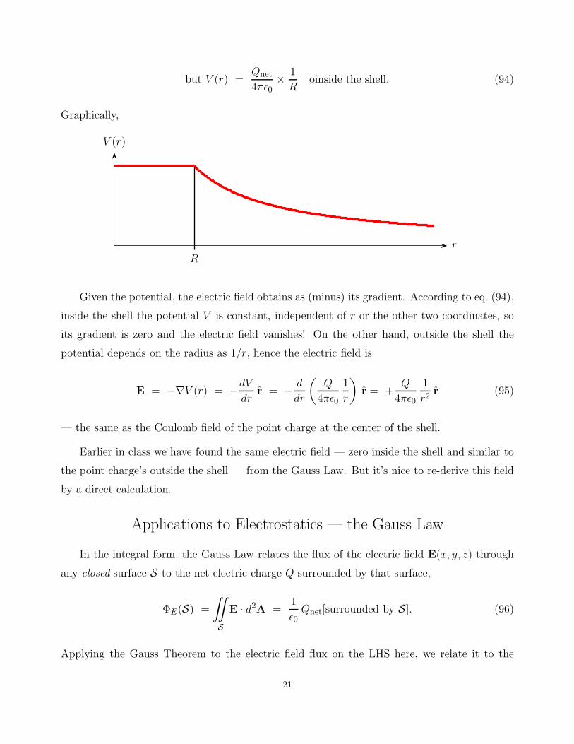
but V (r) =Qnet
4πǫ0× 1
Roinside the shell. (94)
Graphically,
r
V (r)
R
Given the potential, the electric field obtains as (minus) its gradient. According to eq. (94),
inside the shell the potential V is constant, independent of r or the other two coordinates, so
its gradient is zero and the electric field vanishes! On the other hand, outside the shell the
potential depends on the radius as 1/r, hence the electric field is
E = −∇V (r) = −dV
drr = − d
dr
(
Q
4πǫ0
1
r
)
r = +Q
4πǫ0
1
r2r (95)
— the same as the Coulomb field of the point charge at the center of the shell.
Earlier in class we have found the same electric field — zero inside the shell and similar to
the point charge’s outside the shell — from the Gauss Law. But it’s nice to re-derive this field
by a direct calculation.
Applications to Electrostatics — the Gauss Law
In the integral form, the Gauss Law relates the flux of the electric field E(x, y, z) through
any closed surface S to the net electric charge Q surrounded by that surface,
ΦE(S) =
∫∫
S
E · d2A =1
ǫ0Qnet[surrounded by S]. (96)
Applying the Gauss Theorem to the electric field flux on the LHS here, we relate it to the
21

volume integral of the electric field’s divergence,
∫∫∫
V
(∇ · E) d3Vol =
∫∫
S
E · d2A =1
ǫ0Qnet[in V ]. (97)
For a continuous charge distribution with volume density ρ(x, y, z), the net charge on the RHS
obtains as a volume integral
Qnet[in V] =
∫∫∫
V
ρ d3Vol, (98)
hence∫∫∫
V
(∇ · E) d3Vol =1
ǫ0
∫∫∫
V
ρ d3Vol. (99)
Note the volume integrals on both sides of this equation are over the same volume V, whateverit is. Moreover, the equation must hold for any such volume, and this is possible only when the
integrands are equal everywhere in space, point by point:
∀x, y, z : ∇ · E(x, y, z) =1
ǫ0ρ(x, y, z). (100)
This is the Gauss Law in the differential form (in MKSA units).
Altogether, the static electric field has zero curl while its divergence is proportional to the
local electric charge density,
∇× E(x, y, z) ≡ 0, ∇ · E(x, y, z) ≡ 1
ǫ0ρ(x, y, z). (101)
By comparison, the static magnetic field has zero divergence while its curl is proportional to
the local electric current density,
∇ ·B(x, y, z) ≡ 0, ∇×B(x, y, z) = µ0 J(x, y, z). (102)
I shall address the magnetic field later in this class; for now, let’s focus on the electrostatics.
22
Let’s recast the electrostatic equations (101) in terms of the electric potential V (x, y, z).
Note that the very existence of the potential — or rather, the fact that the E(x, y, z) field is a
(minus) gradient of some scalar potential — guarantees zero curl,
E = −∇V =⇒ ∇× E = 0. (103)
Conversely, the Poincare Lemma says (among other things) that if a vector field has zero curl
everywhere, throughout the whole 3D space, then that field is a gradient of some scalar field.
Thus, the zero-curl equation for the electric field assures the existence of the electric potential,
∇×E(x, y, z) ≡ 0 ∀ x, y, z =⇒ ∃V (x, y, z) such that E(x, y, z) = −∇V (x, y, z). (104)
As to the Gauss Law, in terms of the potential, the divergence of the electric field becomes
∇ · E = ∇ · (−∇V ) = −∇2V = −V (105)
where is the Laplacian operator
= ∇2 =∂2
∂x2+
∂2
∂y2+
∂2
∂z2. (106)
Hence, the Gauss Law for the electric field becomes the Poisson equation for the potential,
V (x, y, z) = − 1
ǫ0ρ(x, y, z). (107)
In particular, in empty regions of space where there are no charges, the potential obeys the
Laplace equation
V (x, y, z) = 0. (108)
We shall spend quite a few weeks learning how to solve the Poisson equation and the Laplace
equation for various boundary conditions.
23
Summary
Let me conclude these notes with the summary of essential electrostatic equations in both
MKSA and Gauss units.
• Gauss Law in the integral form:
∫∫
S
E · d2A = Qnet[inside S]×
4π in Gauss units,
1ǫ0
MKSA units.(109)
• Gauss Law in the differential form:
∇ · E(x, y, z) = ρ(x, y, z)×
4π in Gauss units,
1ǫ0
MKSA units.(110)
• Poisson equation:
V (x, y, z) = −ρ(x, y, z)×
4π in Gauss units,
1ǫ0
MKSA units.(111)
• Coulomb potential of a point charge Q:
V (x, y, z) =Q
r×
1 in Gauss units,
14πǫ0
in MKSA units.(112)
• Coulomb electric field of a point charge Q:
V (x, y, z) =Q r
r2×
1 in Gauss units,
14πǫ0
in MKSA units.(113)
⋆ Finally, some equations have similar form in both systems of units:
∇×E(x, y, z) ≡ 0, (114)
E(x, y, z) = −∇V (x, y, z), (115)
V (A) − V (B) =
B∫
A
E · d~ℓ. (116)
24