Gradient Descent Optimization Algorithms for Deep Learning

•Batch gradient descent•Stochastic gradient descent•Mini-batch gradient descent

Slide credit: http://sebastianruder.com/optimizing-gradient-descent/index.html#batchgradientdescent

, ,

, : , : = ∑

∑

SGD=Stochastic GD MomentumNAG=Nesterov accelerated gradientAdagradAdadeltaRMSpropAdam

Notations , , ⋯ , ∈ → input (random variable) having n number of features.

, , ⋯ = labeled dataset with the corresponding target values , , ⋯

=value of feature j in training example , ⋯ ,

, , ⋯ , , = Training set

, , ⋯ , , = Cross validation set

, , ⋯ , , = Test set

Let ∈ be a random variable. ~ , : is distributed as Gaussian (Normal) with mean and variance . Theprobability density function is

; , .

Backpropagation Algorithm

E(W) = ∑

= ∑

The goal is to determine

, , ⋯ , ⇒

, , ⋯ , ⇒

, , ⋯ , ⇒

, , ⋯ , ⇒

such that , , , , , , , ( variables)minimizes the following error

g=Relu

E(W) = ∑

= ∑

g=Relu

To understand Gradient Descent Optimization,

let us consider the following simplified version of the cost function

= , , ⋯ , , ,⋯ ,

Drop g&simplify notationsW=(b,W) X=(1,x)

Its general form

Assume a linear model

, , ⋯ , , , ⋯ , = Hypothesis.

For notational convenience, we may denote , , , ⋯ , ∈ . Here, represents bias and , ⋯ , represents weight vector.

Cost function ∑

Notations

, ,

, : , : = ∑

∑

Gradient Descent Optimization for Linear model

SGD=Stochastic GD MomentumNAG=Nesterov accelerated gradientAdagradAdadeltaRMSpropAdam

Gradient Descent

Cost function ∑

The gradient decent algorithm is Repeat {

⋮

⋮≔

⋮

⋮

⋮∑

⋮(simultaneously update , , ⋯ , )

}(☞ =learning rate)

There are three variants of gradient descent (Batch, Stochastic, Mini-batch), which differ in how much data we use to compute the gradient of the objective function. Depending on the amount of data, we make a trade-off between the accuracy of the parameter update and the time it takes to perform an update.

Quick review of GD & CGD: Solve Let be the residual, which indicates how far we are from the correct value of y. Let f be a function such that .Then where is the error.

GD method is

where is chosen such that 0 ⋅ = ⋅ -y)

Taking -A to , we have , ⋅⋅

CGD method is

where

⋅⋅

, ⋅⋅

CGD method is

where

, ⋅⋅

, ⋅⋅

Mini-batch gradient decent algorithmIf m=Lk& batch =k, for i=0, k, 2k, ….,(L-1)k,

W=W , : , :

Where , : , : = ∑

The advantage of computing more than one example at a time is that we can use vectorized implementations over the k examples.

Map reduce and Data parallelism

1. Divide the training set in to L subsets (z may be the number of machines you have.)

2. On each those machines, calculate , : , :

3. (Map reduce) = , : , : where the data from to are given to the k-th machine.

⋯

Stochastic gradient descent(SGD)From the training set , , ⋯ , , and a given architecture ,

Stochastic gradient descent (SGD) in contrast performs a parameter update for each , :

, , .

The algorithm is as follows:

1. Randomly shuffle the data set

2. Repeat {For , ⋯ , , {

W≔ , ,

}}Here, , , ⋯ , . (1 is for bias b)

: , , may change a lot on each iteration due to the diversity of the training example.

Extensions and variants on SGD Many improvements on the basic SGD algorithm have been proposed and used. In particular, in machine learning, the need to set a learning rate (step size) has been recognized as problematic. Setting this parameter too high can cause the algorithm to diverge; setting it too low makes it slow to converge. A conceptually simple extension of stochastic gradient descent makes the learning rate a decreasing function of the iteration number t, giving a learning rate schedule, so that the first iterations cause large changes in the parameters, while the later ones do only fine-tuning.

SGD=Stochastic GD MomentumNAG=Nesterov accelerated gradientAdagradAdadeltaRMSpropAdam

Momentum: gradient decent algorithm

Stochastic gradient descent with momentum remembers the update at each iteration, and determines the next update as a convex combination of the gradient and the previous update .

Nesterov accelerated gradient

Momentummethod

1.

2. W←

A ball that rolls down a hill, blindly following the slope, is highly unsatisfactory. We'd like to have a smarter ball, a ball that has a notion of where it is going so that it knows to slow down before the hill slopes up again. We set the momentum term to a value of around 0.9. While Momentum first computes the current gradient (small blue vector in Image) and then takes a big jump in the direction of the updated accumulated gradient (big blue vector), NAG first makes a big jump in the direction of the previous accumulated gradient (brown vector), measures the gradient and then makes a correction (red vector), which results in the complete NAG update (green vector). This anticipatory update prevents us from going too fast and results in increased responsiveness, which has significantly increased the performance of RNNs on a number of tasks

NAG uses our momentum term to move . Computing thus gives us an approximation of the next position of . We can now effectively look ahead by calculating the gradient not w.r.t. to our current parameters but w.r.t. the approximate future position

Adagrad

⨀

Adagrad (adaptive gradient) adapts the learning rate to the parameters, performing larger updates for infrequent and smaller updates for frequent parameters.

Adagrad ,

,

,

• , : the gradient of the objective function w.r.t. to parameter at time step t.• ∑ is a diagonal matrix where each diagonal element (i,i) is the sum of the

squares of the gradients w.r.t. W up to time step t. That is, , ∑ ,• A⨀B indicates the element-wise matrix-vector multiplication between A and B:

One of Adagrad's main benefits is that it eliminates the need to manually tune the learning rate. Most implementations use a default value of 0.01 and leave it at that.

Adagrad's main weakness is its accumulation of the squared gradients in the denominator: Since every added term is positive, the accumulated sum keeps growing during training. This in turn causes the learning rate to shrink and eventually become infinitesimally small, at which point the algorithm is no longer able to acquire additional knowledge. The following algorithms aim to resolve this flaw.

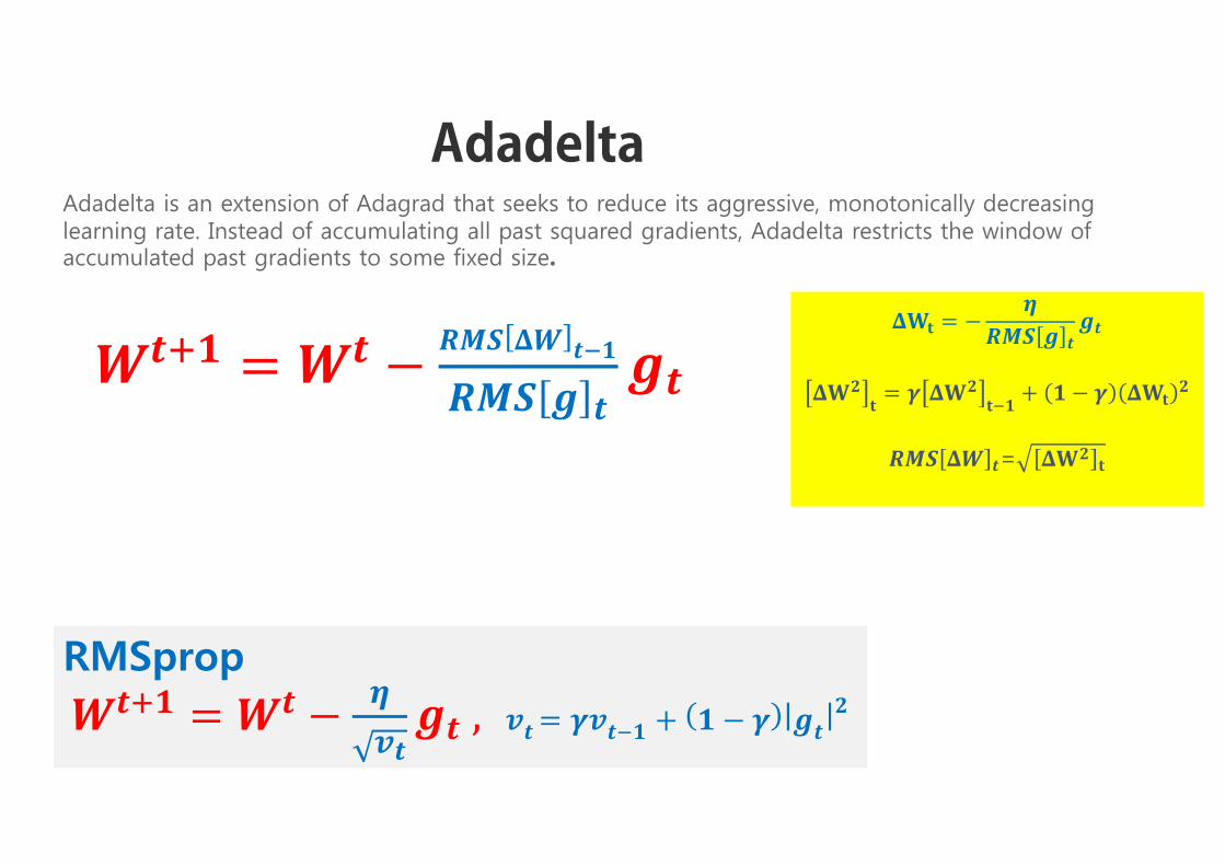
AdadeltaAdadelta is an extension of Adagrad that seeks to reduce its aggressive, monotonically decreasing learning rate. Instead of accumulating all past squared gradients, Adadelta restricts the window of accumulated past gradients to some fixed size.

RMSprop

=

RMSProp

RMSProp (for Root Mean Square Propagation) is also a method in which the learning rate is adapted for each of the parameters. The idea is to divide the learning rate for a weight by a running average of the magnitudes of recent gradients for that weight. RMSprop and Adadelta have both been developed independently around the same time stemming from the need to resolve Adagrad's radically diminishing learning rates. RMSprop in fact is identical to the first update vector of Adadelta

AdamAdaptive Moment Estimation (Adam) is another method that computes adaptive learning rates for each parameter. In addition to storing an exponentially decaying average of past squared gradients like Adadelta and RMSprop, Adam also keeps an exponentially decaying average of past gradients similar to momentum:

Adadelta: , ,

RMSprop: ,

Regularized Least Square

Ridge regression ∑

Lasso ∑

Optimality Theorem

: || ||

,

, ,