gpr inspection of concrete - gssi inc. · geophysical survey systems, inc. concrete handbook gpr...

Copyright © 2001-2017 Geophysical Survey Systems, Inc. All rights reserved including the right of reproduction in whole or in part in any form Published by Geophysical Survey Systems, Inc. 40 Simon Street Nashua, New Hampshire 03060-3075 USA Printed in the United States SIR, RADAN and UtilityScan are registered trademarks of Geophysical Survey Systems, Inc.

Geophysical Survey Systems, Inc. Concrete Handbook GPR Inspection of Concrete

Copyright © 2001-2017 GSSI MN72-367 Rev H

Table of Contents

Introduction ......................................................................................................................................1

Chapter 1: Antenna Characteristics ..........................................................................................3 Antenna – Concrete Interaction ...................................................................................... 3 Transmitter – Receiver (T-R) Offset ................................................................................. 3 Polarization Effects (Antenna Orientation) .................................................................. 4

Chapter 2: Understanding Radar Data ....................................................................................7 Material Properties ............................................................................................................... 7 Layer Reflection ..................................................................................................................... 8 Target Reflection (Hyperbola) ....................................................................................... 10 Feature Identification ....................................................................................................... 14 Using Different Antenna Orientations ....................................................................... 20 Estimating Rebar Diameter ............................................................................................ 22 Penetration Depth ............................................................................................................ 23 Survey Grid Layout ............................................................................................................ 23 Depth Scale Calibration ................................................................................................... 26

Chapter 3: Depth and Position Measurement................................................................... 29 Field Measurement ........................................................................................................... 31 Manual Measurement Using Post-Processing Software ...................................... 32 Automated Measurement .............................................................................................. 32

Chapter 4: 3D Display of Radar Data ..................................................................................... 35 Depth Slice 3D .................................................................................................................... 35 3D QuickDraw and Super 3D ......................................................................................... 36


Copyright © 2001-2017 GSSI 1 MN72-367 Rev H

Introduction This Handbook is intended to “de-mystify” the interpretation of radar data and help you to get the most out of your concrete surveys. It contains basic information on radar theory and method of operation that you would need to understand to perform a survey. The ultimate goal of this guide is to help you to collect good data and interpret that data in order to provide your client with usable information. It explains why and how a certain procedure should be used in a specific case. This guide is only a starting point for you and it is not exhaustive. You will certainly run into situations on the jobsite which are not covered in this guide, but as you gain experience, you will begin to feel more comfortable operating in a variety of situations. It is our hope that the combination of effective training and the tools that you will learn in this guide will start you off in the right direction.

The Handbook mostly deals with what is done BEFORE and AFTER the actual data collection:

• BEFORE: decisions concerning the survey layout, depending on the surveyed structure characteristics, purpose of the survey and equipment capabilities;

• AFTER: data interpretation and decisions concerning data processing.

Structural mapping of concrete is defined here as any application aimed at position or depth determination of anything embedded within a concrete structure. This includes target location (rebar, etc.), measuring thickness of structural layers, and locating voids or fractures that are large enough to be directly detected by a 1.6 GHz, 2.0 GHz, or 2.6 GHz antenna. The principal objectives are target identification and accurate measurement of its position and depth.

We assume here that you are using a GSSI StructureScan™ system with a 1.6 GHz, 2.0 GHz, or 2.6 GHz antenna for your data collection or a 1.6 GHz or 2.6 GHz StructureScan™ Mini, and RADAN® (RAdar Data ANalyzer) processing software for data processing and interpretation.



Chapter 1: Antenna Characteristics The antenna is the crucial element of a radar system. It determines data quality, range resolution, maximum depth of penetration, etc. The 1.6 GHz, 2.0 GHz, and 2.6 GHz antennas used in StructureScan and StructureScan Mini represent the state of the art in high-resolution, shallow penetration, ground-based antennas. They possess the best combination of depth and resolution for the inspection of structural concrete. The basic principles explained below apply to most other bi-static antennas as well. Bi-static refers to the fact that the transmitter and receiver are two separate antenna elements even though they exist within the same enclosure. This differs from a mono-static antenna in that a mono-static uses the same antenna element to transmit and receive signals.

Antenna – Concrete Interaction When you hold your antenna up in the air, it radiates energy within a very wide cone, almost a hemisphere. However, the 1.6/2.0/2.6 GHz and most other GPR antennas are designed to work in contact with or in close proximity to the surface of the concrete. When your antenna is on the concrete, the concrete “pulls” in the antenna’s energy and the antenna becomes coupled to the concrete. To get the best performance, the antenna must stay within 1/10 of the wavelength from the surface – roughly one-half inch for the 1.6 GHz and less for the 2.6 GHz. Increasing the air gap should be avoided because a big air gap will cause most of the radar energy to be reflected off of the concrete surface rather than penetrate.

The direction of the radar energy as it moves into the concrete is mainly determined by the surface of the slab. The signal normally moves perpendicular to the surface, independent of the antenna position. The angle that you hold the antenna over the concrete doesn’t matter. The radar energy will still enter perpendicular to the surface.

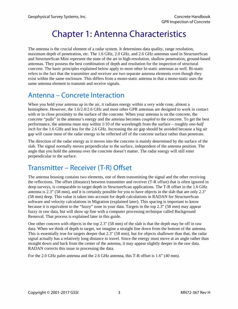
Transmitter – Receiver (T-R) Offset The antenna housing contains two elements, one of them transmitting the signal and the other receiving the reflections. The offset (distance) between transmitter and receiver (T-R offset) that is often ignored in deep surveys, is comparable to target depth in StructureScan applications. The T-R offset in the 1.6 GHz antenna is 2.3” (58 mm), and it is certainly possible for you to have objects in the slab that are only 2.3" (58 mm) deep. This value is taken into account for depth calculations in RADAN for StructureScan software and velocity calculations in Migration (explained later). This spacing is important to know because it is equivalent to the “fuzzy” zone in your data. Targets in the top 2.3” (58 mm) may appear fuzzy in raw data, but will show up fine with a computer processing technique called Background Removal. That process is explained later in this guide.

One other concern with objects in the top 2.3" (58 mm) of the slab is that the depth may be off in raw data. When we think of depth to target, we imagine a straight line down from the bottom of the antenna. This is essentially true for targets deeper that 2.3" (58 mm), but for objects shallower than that, the radar signal actually has a relatively long distance to travel. Since the energy must move at an angle rather than straight down and back from the center of the antenna, it may appear slightly deeper in the raw data. RADAN corrects this issue in processing the data.

For the 2.0 GHz palm antenna and the 2.6 GHz antenna, this T-R offset is 1.6” (40 mm).



Figure 1 shows an antenna over a reflecting rebar.

Transmitter Receiver 1.6 GHz/2.6 GHz antenna (side view)

Surface

Figure 1: Antenna configuration.

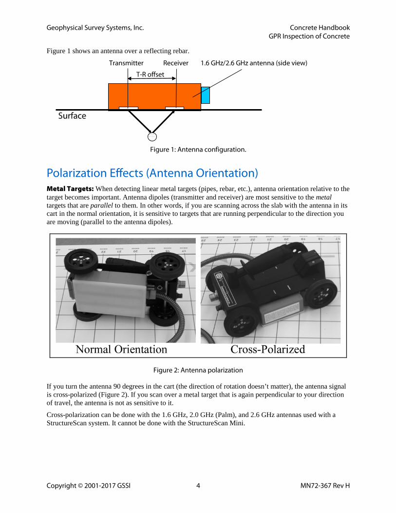
Polarization Effects (Antenna Orientation) Metal Targets: When detecting linear metal targets (pipes, rebar, etc.), antenna orientation relative to the target becomes important. Antenna dipoles (transmitter and receiver) are most sensitive to the metal targets that are parallel to them. In other words, if you are scanning across the slab with the antenna in its cart in the normal orientation, it is sensitive to targets that are running perpendicular to the direction you are moving (parallel to the antenna dipoles).

Figure 2: Antenna polarization

If you turn the antenna 90 degrees in the cart (the direction of rotation doesn’t matter), the antenna signal is cross-polarized (Figure 2). If you scan over a metal target that is again perpendicular to your direction of travel, the antenna is not as sensitive to it.

Cross-polarization can be done with the 1.6 GHz, 2.0 GHz (Palm), and 2.6 GHz antennas used with a StructureScan system. It cannot be done with the StructureScan Mini.

T-R offset



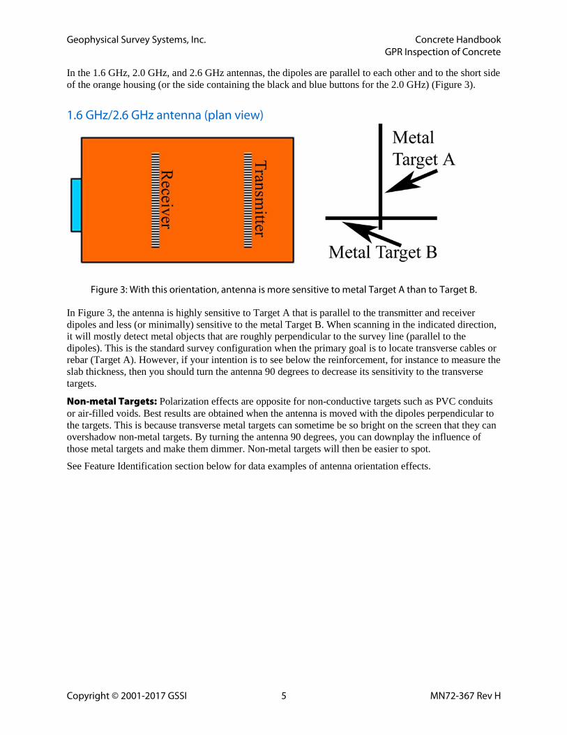
In the 1.6 GHz, 2.0 GHz, and 2.6 GHz antennas, the dipoles are parallel to each other and to the short side of the orange housing (or the side containing the black and blue buttons for the 2.0 GHz) (Figure 3).

1.6 GHz/2.6 GHz antenna (plan view)

Figure 3: With this orientation, antenna is more sensitive to metal Target A than to Target B.

In Figure 3, the antenna is highly sensitive to Target A that is parallel to the transmitter and receiver dipoles and less (or minimally) sensitive to the metal Target B. When scanning in the indicated direction, it will mostly detect metal objects that are roughly perpendicular to the survey line (parallel to the dipoles). This is the standard survey configuration when the primary goal is to locate transverse cables or rebar (Target A). However, if your intention is to see below the reinforcement, for instance to measure the slab thickness, then you should turn the antenna 90 degrees to decrease its sensitivity to the transverse targets.

Non-metal Targets: Polarization effects are opposite for non-conductive targets such as PVC conduits or air-filled voids. Best results are obtained when the antenna is moved with the dipoles perpendicular to the targets. This is because transverse metal targets can sometime be so bright on the screen that they can overshadow non-metal targets. By turning the antenna 90 degrees, you can downplay the influence of those metal targets and make them dimmer. Non-metal targets will then be easier to spot.

See Feature Identification section below for data examples of antenna orientation effects.



Chapter 2: Understanding Radar Data

Material Properties Radar energy responds to different materials in different ways. The way that it responds to each material is governed by two physical properties of the material. The first one is electrical conductivity. Since GPR is EM energy, it is subject to attenuation (natural absorption) as it moves through a material. If the energy is moving through a resistive (low conductivity) material such as very dry sand, ice, or dry concrete, the signal is able to penetrate a great deal of material. This is because the signal stays intact longer and is thus able to go further into the material. If a material is conductive (salt water, wet concrete), the GPR energy will get absorbed before it has had the chance to go very far into the material. As a result, radar is suitable for inspection of any material with low electrical conductivity (concrete, sand, wood, asphalt, etc.). As a rule of thumb, the greater the water content of the material, the greater the conductivity. In a practical sense, what this means is that you will see deeper in old, dry concrete than you will in concrete that is not well cured.

The other important physical property is the dielectric constant. The dielectric contrast is a descriptive number that indicates, among other things, how fast radar energy travels through a material. Radar energy will always move as quickly as possible through a material, but certain materials slow the energy more than others. If we know the dielectric of the concrete, we can figure out how deep something is because the dielectric tells us how fast the GPR energy is moving. Your radar is measuring how long it took to get the reflection, so if we know the speed of the energy, your radar can multiply the two-way travel time and speed to get depth. The higher the dielectric, the slower the radar wave moves through the medium, and vice versa. The range of values goes from 1 (air) to 81 (water). GPR energy moves through air at almost the speed of light. It moves though water at about 1/9 the speed of light. A dielectric of 3 to 12, typical for construction materials, corresponds to radar velocities from 7 to 3.5 inches per nanosecond (or 18 to 9 cm per nanosecond), respectively. Wet materials will slow down the radar signal because the presence of the water will raise the overall dielectric of the material.

The other important reason we focus on dielectrics is that for a reflection to be produced, there must be a contrast in the dielectric value of the material that the signal is going through and the dielectric of the target. In other words, a reflection is produced at a boundary between two different materials, where the dielectric (and the signal velocity) suddenly changes. A higher dielectric contrast, or difference in dielectric between the two materials, results in a stronger reflection.

Additionally, the contrast in electrical conductivity between the material you are scanning through and the target will affect the brightness of the reflection. Metal targets show as very bright reflections because they are conductive. In addition to the reflected radar wave, metal targets will return a small extra signal that results from them becoming charged. Non-metal, non-conductive targets will only return the reflected energy.

Metal, even as thin as aluminum foil, is a complete reflector of radar energy. The reflection from it is clearly visible, but the targets behind it will not be detected. A fine wire mesh (2x2", 5x5 cm or smaller) acts like sheet metal and is impenetrable. You will not see targets beneath such a tight mesh.

The strength (brightness) of a reflection is proportional to the dielectric contrast between the two materials. The greater the contrast, the brighter the reflection (examples follow):



Table 1.

Boundary Dielectric Contrast Reflection Strength

Asphalt - Concrete Medium Medium

Concrete - Sand Low Weak

Concrete - Air High, phase reversal Strong

Concrete Deck - Concrete Beam None No reflection

Concrete - Metal High Strong

Concrete - Water High Strong

Concrete - PVC Low to Medium, phase reversal Weak

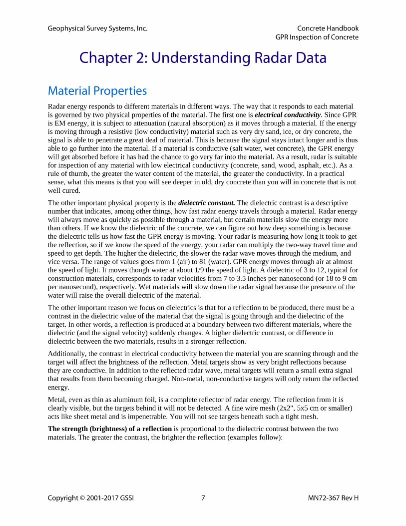
Reflection Polarity will tell you a great deal about the type of material a reflection comes from. They come in two forms: Positive and Negative (White and Black in the default color table). This color will be distinguished by whatever the first most dominant band is in your hyperbola. There will usually be a weaker band of the opposite color on top of the first dominant band. There will also be a strong band of the opposite color below the first dominant band. This “halo” effect is just an imperfection in the received signal.

Figure 4: Metal and PVC targets. Reflection polarity.

A negative reflection tells you that the radar wave sped up when it reached an object. Often in a concrete or structure scan this means that your hyperbola has reflected off of an air filled PVC or an air void. A radar wave will travel fastest through air.

Air-filled PVC

Metal

“Halo” Effect

Dominant Band

“Halo” Effect



A positive reflection tells you that the radar wave has slowed down. In a concrete or structure scan, this usually means that you received a reflection off of a metal object. This metal object could be rebar, a PT cable, a metal conduit, etc. A single reflection won’t tell you exactly what the object is, just a general idea of what the object may be. From here, you have to bring in your own knowledge about the area.

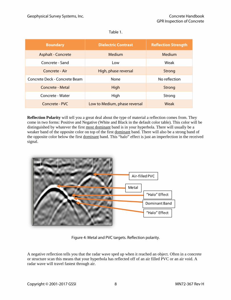
Layer Reflection When scanning over a continuous layer boundary (asphalt-concrete, concrete-subgrade, etc.), the antenna repeatedly receives reflections from sections of that boundary within the antenna footprint. They form a layer reflection that resembles the reflecting boundary.

Concrete Bottom



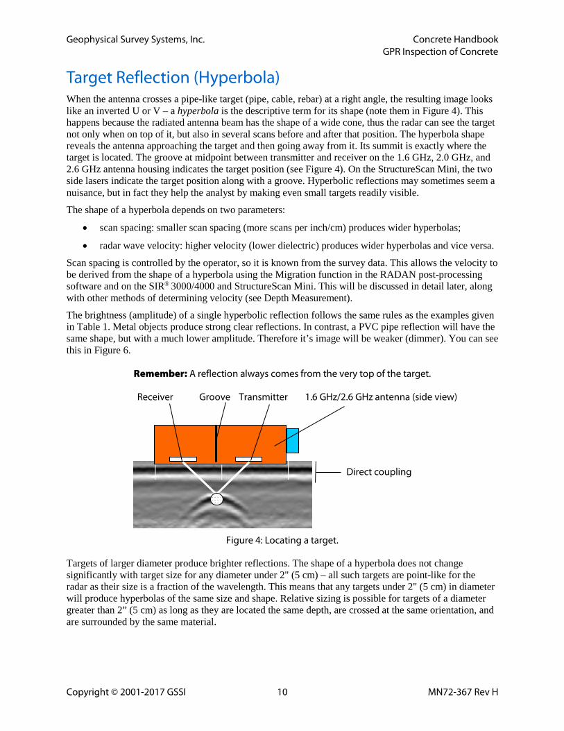
Target Reflection (Hyperbola) When the antenna crosses a pipe-like target (pipe, cable, rebar) at a right angle, the resulting image looks like an inverted U or V – a hyperbola is the descriptive term for its shape (note them in Figure 4). This happens because the radiated antenna beam has the shape of a wide cone, thus the radar can see the target not only when on top of it, but also in several scans before and after that position. The hyperbola shape reveals the antenna approaching the target and then going away from it. Its summit is exactly where the target is located. The groove at midpoint between transmitter and receiver on the 1.6 GHz, 2.0 GHz, and 2.6 GHz antenna housing indicates the target position (see Figure 4). On the StructureScan Mini, the two side lasers indicate the target position along with a groove. Hyperbolic reflections may sometimes seem a nuisance, but in fact they help the analyst by making even small targets readily visible.

The shape of a hyperbola depends on two parameters:

• scan spacing: smaller scan spacing (more scans per inch/cm) produces wider hyperbolas;

• radar wave velocity: higher velocity (lower dielectric) produces wider hyperbolas and vice versa.

Scan spacing is controlled by the operator, so it is known from the survey data. This allows the velocity to be derived from the shape of a hyperbola using the Migration function in the RADAN post-processing software and on the SIR® 3000/4000 and StructureScan Mini. This will be discussed in detail later, along with other methods of determining velocity (see Depth Measurement).

The brightness (amplitude) of a single hyperbolic reflection follows the same rules as the examples given in Table 1. Metal objects produce strong clear reflections. In contrast, a PVC pipe reflection will have the same shape, but with a much lower amplitude. Therefore it’s image will be weaker (dimmer). You can see this in Figure 6.

Remember: A reflection always comes from the very top of the target.

Receiver Groove Transmitter 1.6 GHz/2.6 GHz antenna (side view)

Figure 4: Locating a target.

Targets of larger diameter produce brighter reflections. The shape of a hyperbola does not change significantly with target size for any diameter under 2" (5 cm) – all such targets are point-like for the radar as their size is a fraction of the wavelength. This means that any targets under 2" (5 cm) in diameter will produce hyperbolas of the same size and shape. Relative sizing is possible for targets of a diameter greater than 2” (5 cm) as long as they are located the same depth, are crossed at the same orientation, and are surrounded by the same material.

Direct coupling



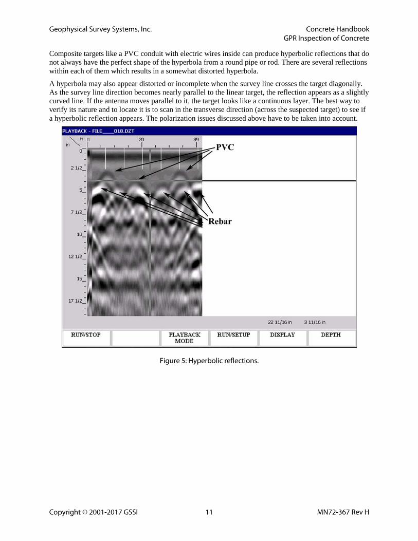
Composite targets like a PVC conduit with electric wires inside can produce hyperbolic reflections that do not always have the perfect shape of the hyperbola from a round pipe or rod. There are several reflections within each of them which results in a somewhat distorted hyperbola.

A hyperbola may also appear distorted or incomplete when the survey line crosses the target diagonally. As the survey line direction becomes nearly parallel to the linear target, the reflection appears as a slightly curved line. If the antenna moves parallel to it, the target looks like a continuous layer. The best way to verify its nature and to locate it is to scan in the transverse direction (across the suspected target) to see if a hyperbolic reflection appears. The polarization issues discussed above have to be taken into account.

Figure 5: Hyperbolic reflections.



Target Detection Accuracy

Horizontal Accuracy and Resolution The accuracy with which we can locate a target depends on the antenna pattern and scan spacing. If the antenna were radiating a narrow vertical beam, we would see a small dot-like image of the target right where it is located. Instead, it radiates in a cone approximately 60 degrees wide. The antenna starts sensing the target when approaching it, continues to receive reflections as it passes over and for some distance past the target. The range between antenna and target changes as it moves, which explains the hyperbolic shape of the reflection.

The target is located at the peak of the hyperbola (see Figure 4). Thus it is critical how accurately the hyperbola summit can be located. The positioning accuracy is approximately equal to the scan spacing, but does not get finer than ¼" (6 mm) under any conditions.

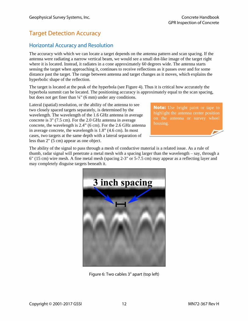
Lateral (spatial) resolution, or the ability of the antenna to see two closely spaced targets separately, is determined by the wavelength. The wavelength of the 1.6 GHz antenna in average concrete is 3" (7.5 cm). For the 2.0 GHz antenna in average concrete, the wavelength is 2.4” (6 cm). For the 2.6 GHz antenna in average concrete, the wavelength is 1.8” (4.6 cm). In most cases, two targets at the same depth with a lateral separation of less than 2" (5 cm) appear as one object.

The ability of the signal to pass through a mesh of conductive material is a related issue. As a rule of thumb, radar signal will penetrate a metal mesh with a spacing larger than the wavelength – say, through a 6" (15 cm) wire mesh. A fine metal mesh (spacing 2-3" or 5-7.5 cm) may appear as a reflecting layer and may completely disguise targets beneath it.

Figure 6: Two cables 3" apart (top left)

Note: Use bright paint or tape to highlight the antenna center position on the antenna or survey wheel housing.



Range (Depth) Accuracy and Resolution StructureScan and StructureScan Mini are capable of measuring depth to a target in ¼” (6 mm) increments – this is its absolute accuracy. The resulting depth readout will be accurate to ¼" (6 mm or 5% of the depth, whichever is greater) if a depth calibration procedure has been correctly performed prior to the measurement. When an assumed Concrete Type is used, the measured depth can be off by as much as 20%.

Vertically, a distance of ¼ of the wavelength between two targets is sufficient to see them separately which yields a range resolution of less than one inch. The deeper target can still be invisible if it is directly beneath the top target or in close proximity (less than 1" or 2.5 cm horizontal separation).

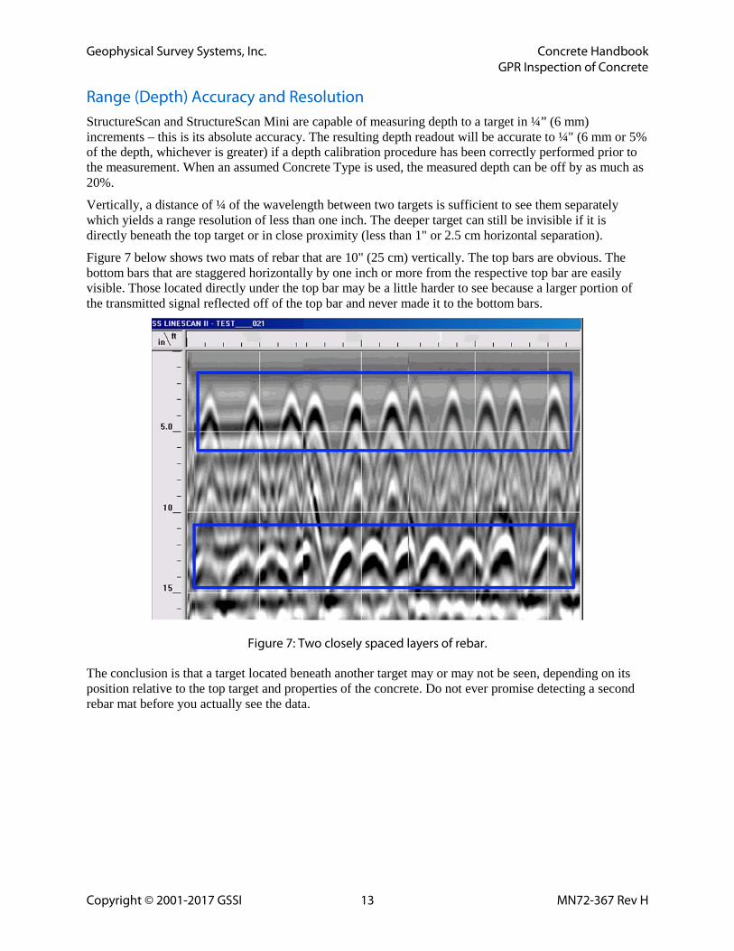
Figure 7 below shows two mats of rebar that are 10" (25 cm) vertically. The top bars are obvious. The bottom bars that are staggered horizontally by one inch or more from the respective top bar are easily visible. Those located directly under the top bar may be a little harder to see because a larger portion of the transmitted signal reflected off of the top bar and never made it to the bottom bars.

Figure 7: Two closely spaced layers of rebar.

The conclusion is that a target located beneath another target may or may not be seen, depending on its position relative to the top target and properties of the concrete. Do not ever promise detecting a second rebar mat before you actually see the data.

1

1



Feature Identification

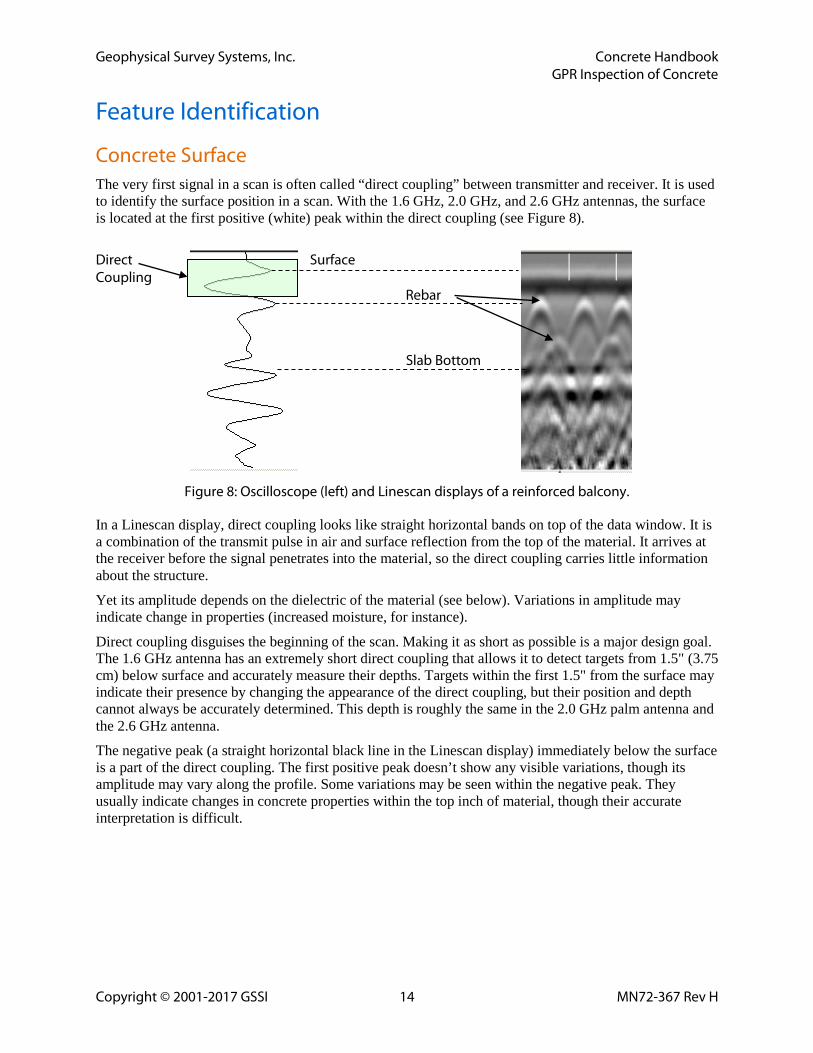
Concrete Surface The very first signal in a scan is often called “direct coupling” between transmitter and receiver. It is used to identify the surface position in a scan. With the 1.6 GHz, 2.0 GHz, and 2.6 GHz antennas, the surface is located at the first positive (white) peak within the direct coupling (see Figure 8).

Direct Surface Coupling

Rebar

Figure 8: Oscilloscope (left) and Linescan displays of a reinforced balcony.

In a Linescan display, direct coupling looks like straight horizontal bands on top of the data window. It is a combination of the transmit pulse in air and surface reflection from the top of the material. It arrives at the receiver before the signal penetrates into the material, so the direct coupling carries little information about the structure.

Yet its amplitude depends on the dielectric of the material (see below). Variations in amplitude may indicate change in properties (increased moisture, for instance).

Direct coupling disguises the beginning of the scan. Making it as short as possible is a major design goal. The 1.6 GHz antenna has an extremely short direct coupling that allows it to detect targets from 1.5" (3.75 cm) below surface and accurately measure their depths. Targets within the first 1.5" from the surface may indicate their presence by changing the appearance of the direct coupling, but their position and depth cannot always be accurately determined. This depth is roughly the same in the 2.0 GHz palm antenna and the 2.6 GHz antenna.

The negative peak (a straight horizontal black line in the Linescan display) immediately below the surface is a part of the direct coupling. The first positive peak doesn’t show any visible variations, though its amplitude may vary along the profile. Some variations may be seen within the negative peak. They usually indicate changes in concrete properties within the top inch of material, though their accurate interpretation is difficult.

Slab Bottom



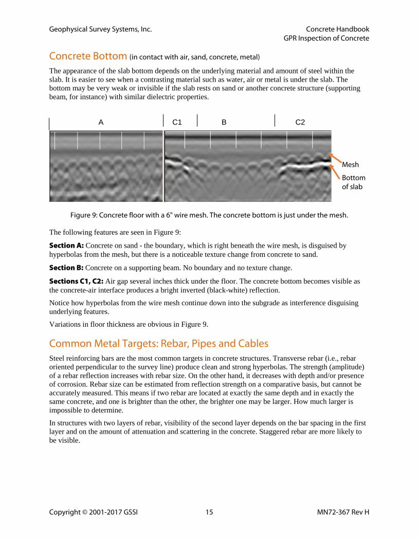
Concrete Bottom (in contact with air, sand, concrete, metal)

The appearance of the slab bottom depends on the underlying material and amount of steel within the slab. It is easier to see when a contrasting material such as water, air or metal is under the slab. The bottom may be very weak or invisible if the slab rests on sand or another concrete structure (supporting beam, for instance) with similar dielectric properties.

A C1 B C2

Figure 9: Concrete floor with a 6" wire mesh. The concrete bottom is just under the mesh.

The following features are seen in Figure 9:

Section A: Concrete on sand - the boundary, which is right beneath the wire mesh, is disguised by hyperbolas from the mesh, but there is a noticeable texture change from concrete to sand.

Section B: Concrete on a supporting beam. No boundary and no texture change.

Sections C1, C2: Air gap several inches thick under the floor. The concrete bottom becomes visible as the concrete-air interface produces a bright inverted (black-white) reflection.

Notice how hyperbolas from the wire mesh continue down into the subgrade as interference disguising underlying features.

Variations in floor thickness are obvious in Figure 9.

Common Metal Targets: Rebar, Pipes and Cables Steel reinforcing bars are the most common targets in concrete structures. Transverse rebar (i.e., rebar oriented perpendicular to the survey line) produce clean and strong hyperbolas. The strength (amplitude) of a rebar reflection increases with rebar size. On the other hand, it decreases with depth and/or presence of corrosion. Rebar size can be estimated from reflection strength on a comparative basis, but cannot be accurately measured. This means if two rebar are located at exactly the same depth and in exactly the same concrete, and one is brighter than the other, the brighter one may be larger. How much larger is impossible to determine.

In structures with two layers of rebar, visibility of the second layer depends on the bar spacing in the first layer and on the amount of attenuation and scattering in the concrete. Staggered rebar are more likely to be visible.

Mesh

Bottom of slab



A steel pipe (conduit, for instance) looks exactly the same as a steel rebar of the same diameter. The radar signal does not penetrate metal, so there is no difference between reflections from a solid rod or a hollow metallic pipe. A large diameter conduit, duct or pipe (over 2" or 5 cm) will have a noticeable horizontal size in the profile, but it is still unwise to attempt to find the size of the target from your radar data.

Figure 10: Two rebar mats (Elevated slab - balcony).

Post-tensioned steel cables are present in some structures along with reinforcing bars. Their appearance in a radar profile is similar to that of a rebar. Radar does not have adequate resolution to differentiate strands in a cable. An uncoated steel cable and a rebar of the same size would look identical. In real structures, cables are placed into plastic conduits and/or coated with plastic, which may affect the reflection strength.

The only reliable way to identify conduits and cables is to trace them in several radar profiles (3D display is highly recommended for this task). Their direction, depth and continuity allow them to be differentiated from rebar.

Figure 11: Two cables located above the rebar mat – vertical profile and plan view.

Surface Top rebar Bottom rebar Bottom of slab (concrete-air interface)



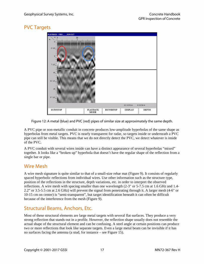
PVC Targets

Figure 12: A metal (blue) and PVC (red) pipes of similar size at approximately the same depth.

A PVC pipe or non-metallic conduit in concrete produces low-amplitude hyperbolas of the same shape as hyperbolas from metal targets. PVC is nearly transparent for radar, so targets inside or underneath a PVC pipe can still be visible. This means that we do not directly detect the PVC, we detect whatever is inside of the PVC.

A PVC conduit with several wires inside can have a distinct appearance of several hyperbolas “mixed” together. It looks like a “broken up” hyperbola that doesn’t have the regular shape of the reflection from a single bar or pipe.

Wire Mesh A wire mesh signature is quite similar to that of a small-size rebar mat (Figure 9). It consists of regularly spaced hyperbolic reflections from individual wires. Use other information such as the structure type, position of the reflections in the structure, depth variations, etc. in order to interpret the observed reflections. A wire mesh with spacing smaller than one wavelength (2-3" or 5-7.5 cm at 1.6 GHz and 1.4-2.2” or 3.5-5.5 cm at 2.6 GHz) will prevent the signal from penetrating through it. A larger mesh (4-6" or 10-15 cm on center) is “semi-transparent”, but target identification beneath it can often be difficult because of the interference from the mesh (Figure 9).

Structural Beams, Anchors, Etc. Most of these structural elements are large metal targets with several flat surfaces. They produce a very strong reflection that stands out in a profile. However, the reflection shape usually does not resemble the actual shape of the structural element and can be confusing. A steel angle at certain positions can produce two or more reflections that look like separate targets. Even a large metal beam can be invisible if it has no surfaces facing the antenna (a stud, for instance – see Figure 15).



The general guidelines for “deciphering” these reflections are as follows:

• A flat surface wider than 2" (5 cm) will appear flat, with hyperbolic “wings” dropping off both ends;

• A reflection will arrive from the part of the target nearest to the antenna;

• Vertical surfaces will not show up;

• Parts that are “hidden” behind other reflecting surfaces, will not show up.

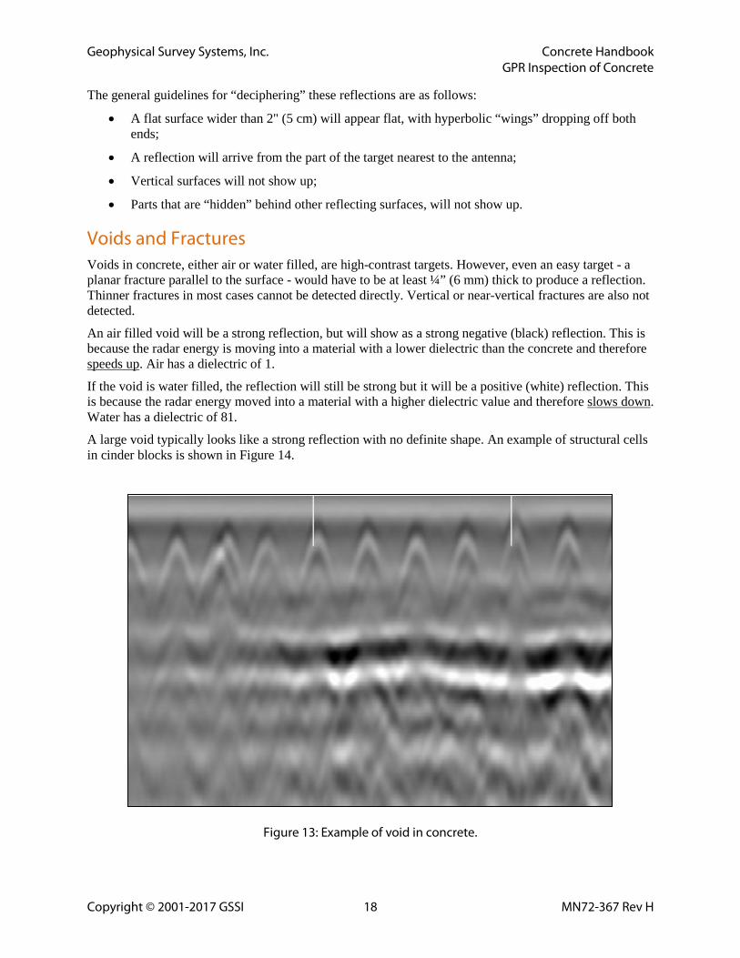
Voids and Fractures Voids in concrete, either air or water filled, are high-contrast targets. However, even an easy target - a planar fracture parallel to the surface - would have to be at least ¼” (6 mm) thick to produce a reflection. Thinner fractures in most cases cannot be detected directly. Vertical or near-vertical fractures are also not detected.

An air filled void will be a strong reflection, but will show as a strong negative (black) reflection. This is because the radar energy is moving into a material with a lower dielectric than the concrete and therefore speeds up. Air has a dielectric of 1.

If the void is water filled, the reflection will still be strong but it will be a positive (white) reflection. This is because the radar energy moved into a material with a higher dielectric value and therefore slows down. Water has a dielectric of 81.

A large void typically looks like a strong reflection with no definite shape. An example of structural cells in cinder blocks is shown in Figure 14.

Figure 13: Example of void in concrete.



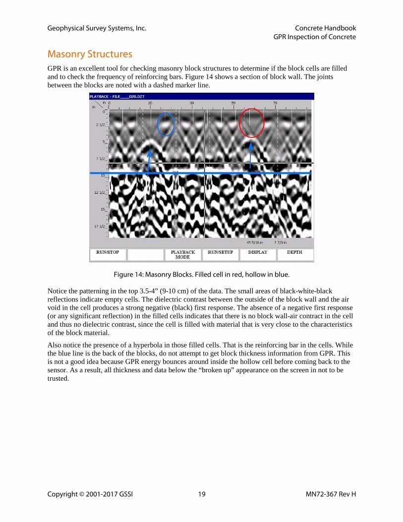
Masonry Structures GPR is an excellent tool for checking masonry block structures to determine if the block cells are filled and to check the frequency of reinforcing bars. Figure 14 shows a section of block wall. The joints between the blocks are noted with a dashed marker line.

Figure 14: Masonry Blocks. Filled cell in red, hollow in blue.

Notice the patterning in the top 3.5-4” (9-10 cm) of the data. The small areas of black-white-black reflections indicate empty cells. The dielectric contrast between the outside of the block wall and the air void in the cell produces a strong negative (black) first response. The absence of a negative first response (or any significant reflection) in the filled cells indicates that there is no block wall-air contract in the cell and thus no dielectric contrast, since the cell is filled with material that is very close to the characteristics of the block material.

Also notice the presence of a hyperbola in those filled cells. That is the reinforcing bar in the cells. While the blue line is the back of the blocks, do not attempt to get block thickness information from GPR. This is not a good idea because GPR energy bounces around inside the hollow cell before coming back to the sensor. As a result, all thickness and data below the “broken up” appearance on the screen in not to be trusted.



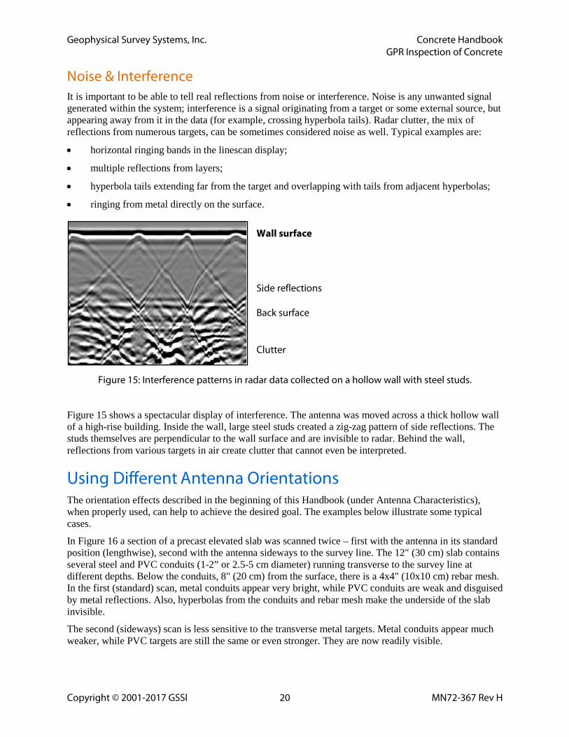
Noise & Interference It is important to be able to tell real reflections from noise or interference. Noise is any unwanted signal generated within the system; interference is a signal originating from a target or some external source, but appearing away from it in the data (for example, crossing hyperbola tails). Radar clutter, the mix of reflections from numerous targets, can be sometimes considered noise as well. Typical examples are:

• horizontal ringing bands in the linescan display;

• multiple reflections from layers;

• hyperbola tails extending far from the target and overlapping with tails from adjacent hyperbolas;

• ringing from metal directly on the surface.

Wall surface

Side reflections Back surface Clutter

Figure 15: Interference patterns in radar data collected on a hollow wall with steel studs.

Figure 15 shows a spectacular display of interference. The antenna was moved across a thick hollow wall of a high-rise building. Inside the wall, large steel studs created a zig-zag pattern of side reflections. The studs themselves are perpendicular to the wall surface and are invisible to radar. Behind the wall, reflections from various targets in air create clutter that cannot even be interpreted.

Using Different Antenna Orientations The orientation effects described in the beginning of this Handbook (under Antenna Characteristics), when properly used, can help to achieve the desired goal. The examples below illustrate some typical cases.

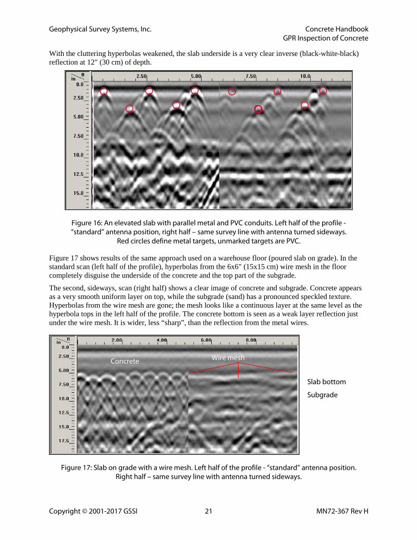
In Figure 16 a section of a precast elevated slab was scanned twice – first with the antenna in its standard position (lengthwise), second with the antenna sideways to the survey line. The 12" (30 cm) slab contains several steel and PVC conduits (1-2” or 2.5-5 cm diameter) running transverse to the survey line at different depths. Below the conduits, 8" (20 cm) from the surface, there is a 4x4" (10x10 cm) rebar mesh. In the first (standard) scan, metal conduits appear very bright, while PVC conduits are weak and disguised by metal reflections. Also, hyperbolas from the conduits and rebar mesh make the underside of the slab invisible.

The second (sideways) scan is less sensitive to the transverse metal targets. Metal conduits appear much weaker, while PVC targets are still the same or even stronger. They are now readily visible.



With the cluttering hyperbolas weakened, the slab underside is a very clear inverse (black-white-black) reflection at 12" (30 cm) of depth.

Figure 16: An elevated slab with parallel metal and PVC conduits. Left half of the profile - “standard” antenna position, right half – same survey line with antenna turned sideways.

Red circles define metal targets, unmarked targets are PVC.

Figure 17 shows results of the same approach used on a warehouse floor (poured slab on grade). In the standard scan (left half of the profile), hyperbolas from the 6x6" (15x15 cm) wire mesh in the floor completely disguise the underside of the concrete and the top part of the subgrade.

The second, sideways, scan (right half) shows a clear image of concrete and subgrade. Concrete appears as a very smooth uniform layer on top, while the subgrade (sand) has a pronounced speckled texture. Hyperbolas from the wire mesh are gone; the mesh looks like a continuous layer at the same level as the hyperbola tops in the left half of the profile. The concrete bottom is seen as a weak layer reflection just under the wire mesh. It is wider, less “sharp”, than the reflection from the metal wires.

Figure 17: Slab on grade with a wire mesh. Left half of the profile - “standard” antenna position. Right half – same survey line with antenna turned sideways.

Concrete Wire mesh

Slab bottom

Subgrade



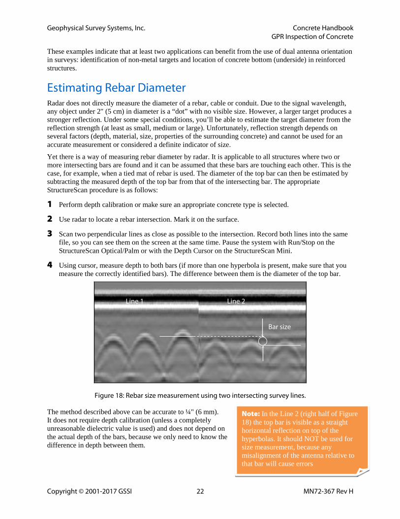
Note: In the Line 2 (right half of Figure 18) the top bar is visible as a straight horizontal reflection on top of the hyperbolas. It should NOT be used for size measurement, because any misalignment of the antenna relative to that bar will cause errors

These examples indicate that at least two applications can benefit from the use of dual antenna orientation in surveys: identification of non-metal targets and location of concrete bottom (underside) in reinforced structures.

Estimating Rebar Diameter Radar does not directly measure the diameter of a rebar, cable or conduit. Due to the signal wavelength, any object under 2" (5 cm) in diameter is a “dot” with no visible size. However, a larger target produces a stronger reflection. Under some special conditions, you’ll be able to estimate the target diameter from the reflection strength (at least as small, medium or large). Unfortunately, reflection strength depends on several factors (depth, material, size, properties of the surrounding concrete) and cannot be used for an accurate measurement or considered a definite indicator of size.

Yet there is a way of measuring rebar diameter by radar. It is applicable to all structures where two or more intersecting bars are found and it can be assumed that these bars are touching each other. This is the case, for example, when a tied mat of rebar is used. The diameter of the top bar can then be estimated by subtracting the measured depth of the top bar from that of the intersecting bar. The appropriate StructureScan procedure is as follows:

1 Perform depth calibration or make sure an appropriate concrete type is selected.

2 Use radar to locate a rebar intersection. Mark it on the surface.

3 Scan two perpendicular lines as close as possible to the intersection. Record both lines into the same file, so you can see them on the screen at the same time. Pause the system with Run/Stop on the StructureScan Optical/Palm or with the Depth Cursor on the StructureScan Mini.

4 Using cursor, measure depth to both bars (if more than one hyperbola is present, make sure that you measure the correctly identified bars). The difference between them is the diameter of the top bar.

Figure 18: Rebar size measurement using two intersecting survey lines.

The method described above can be accurate to ¼" (6 mm). It does not require depth calibration (unless a completely unreasonable dielectric value is used) and does not depend on the actual depth of the bars, because we only need to know the difference in depth between them.

Bar size

Line 1 Line 2



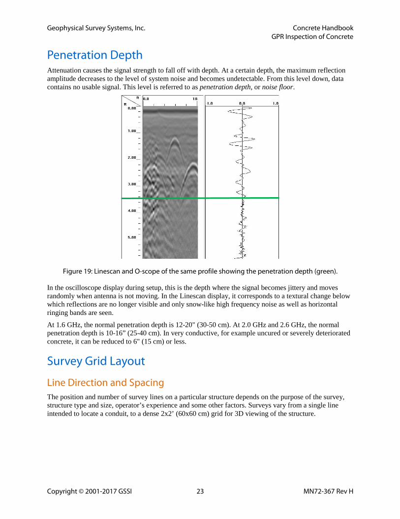
Penetration Depth Attenuation causes the signal strength to fall off with depth. At a certain depth, the maximum reflection amplitude decreases to the level of system noise and becomes undetectable. From this level down, data contains no usable signal. This level is referred to as penetration depth, or noise floor.

Figure 19: Linescan and O-scope of the same profile showing the penetration depth (green).

In the oscilloscope display during setup, this is the depth where the signal becomes jittery and moves randomly when antenna is not moving. In the Linescan display, it corresponds to a textural change below which reflections are no longer visible and only snow-like high frequency noise as well as horizontal ringing bands are seen.

At 1.6 GHz, the normal penetration depth is 12-20" (30-50 cm). At 2.0 GHz and 2.6 GHz, the normal penetration depth is 10-16” (25-40 cm). In very conductive, for example uncured or severely deteriorated concrete, it can be reduced to 6" (15 cm) or less.

Survey Grid Layout

Line Direction and Spacing The position and number of survey lines on a particular structure depends on the purpose of the survey, structure type and size, operator’s experience and some other factors. Surveys vary from a single line intended to locate a conduit, to a dense 2x2’ (60x60 cm) grid for 3D viewing of the structure.



The general guidelines are as follows:

• Plan survey lines so they cross perpendicularly the features you intend to detect.

• A line spacing of 2-3" (5-7.5 cm) is required for complete coverage. This is the maximum practicable survey density that may be used for a detailed 3D mapping, for example.

• Line spacing of 6" (15 cm) to 12" (30 cm) is adequate for most concrete mapping purposes.

• Linear targets that cross the survey lines at an angle of 45 to 90 degrees, will be resolved with good accuracy. A complete survey of the structure (to clear locations for drilling, cutting or coring, for example) requires a survey in two perpendicular directions.

• To clear a spot for drilling within a small area, use at least a “tic-tac-toe” pattern with a minimum of four lines. This will determine position and direction of the structural elements.

It may be useful to do a couple of preliminary scans to determine the position of main reinforcing elements. Mark them on the surface and then lay out the grid accordingly.

Position (Distance) Control The antenna position along each survey line (distance scale) is controlled either with a survey wheel or by manual marking. The survey wheel has an encoder that sends a fixed number of pulses per revolution to the control unit. The control unit then uses these pulses to trigger the antenna at equal distance intervals (scan spacing). In StructureScan and StructureScan Mini, these intervals are dependent on the scans per unit setting selected by the operator.

The survey wheel is the recommended method of distance control. When a survey wheel is not available or cannot be used for some reason, the only way of maintaining distance control is to mark the surface at even intervals (or use existing visible marks such as tile edges) and then enter user marks at these locations. The scan spacing will vary along the line and will have to be corrected using Distance Normalization in the RADAN post-processing software. To do this, you need to know the exact distance between markers. This method of collection cannot be done with the StructureScan Mini, but can be done with StructureScan.

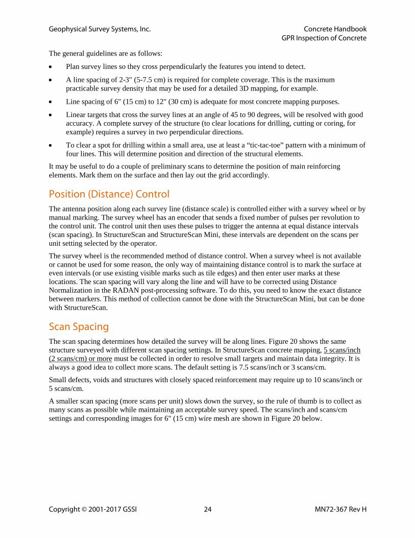
Scan Spacing The scan spacing determines how detailed the survey will be along lines. Figure 20 shows the same structure surveyed with different scan spacing settings. In StructureScan concrete mapping, 5 scans/inch (2 scans/cm) or more must be collected in order to resolve small targets and maintain data integrity. It is always a good idea to collect more scans. The default setting is 7.5 scans/inch or 3 scans/cm.

Small defects, voids and structures with closely spaced reinforcement may require up to 10 scans/inch or 5 scans/cm.

A smaller scan spacing (more scans per unit) slows down the survey, so the rule of thumb is to collect as many scans as possible while maintaining an acceptable survey speed. The scans/inch and scans/cm settings and corresponding images for 6" (15 cm) wire mesh are shown in Figure 20 below.



Figure 20: Scan spacing effects.

Survey Wheel Accuracy Under optimal conditions (smooth surface, proper calibration, no slippage) survey wheel distance error does not exceed +2% (+2 ft or 60 cm over a 100 ft or 30 m distance). If a better accuracy is desired, we recommend inserting a user mark at the end of the measured survey line. In RADAN, there are two ways of correcting the distance scale using the start and end marks:

• If the exact scan spacing does not matter - adjust the scan/unit parameter in the file header so the indicated distance between the marks equals the true distance. Survey wheel accuracy decreases on a rough or dirty surface and at a higher speed.

• If a certain scan spacing should be kept, you will need to use the Distance Normalization procedure using the exact Start - End mark distance and the desired Scan/Unit value. This procedure requires the RADAN software. See the RADAN manual for instructions on this procedure.

Manual Marking Surveying without a survey wheel is not recommended. However, user markers (vertical dashed lines in the data) help to establish a distance scale when using a survey wheel is impossible or impractical. They can be entered by clicking the marker button on the control unit. Distance Normalization based on properly entered user markers can render a distance scale with an average accuracy as good as the one obtained with a survey wheel. However, individual scan spacing may be different which causes uncontrolled local position errors.

Mark the surface with chalk or paint at equal intervals prior to surveying. The mark spacing (distance units per mark) should be 10 times the acceptable error or smaller. If an inch or cm accuracy is sought, marks should be entered every 10 inches or 10 cm, while a 10 ft or 10 m mark spacing is sufficient to provide a 1 ft or 1 m accuracy. User markers are entered each time the antenna center crosses a painted line.



When surveying without a survey wheel, the operator should move the antenna at a steady speed, avoiding stops and jerks. Also, the scan spacing depends on the antenna speed and no warning is given if the antenna moves too fast. The optimal speed should be calculated from the desired scan spacing and known system scan rate:

Speed (ft/sec) = (Scan Spacing) x (Scan Rate)

A few test lines should be taken to determine optimal speed from the visual appearance of the data (Figure 20).

Depth Scale Calibration Surface identification: Accurate surface identification is the first step to a correct depth scale. Most GPR systems do not automatically locate the surface. The time (and depth) scale starts at an arbitrary time-zero, usually above the true surface. This has to be taken into consideration and corrected. In RADAN for StructureScan and RADAN® for StructureScan Mini, this process can be done automatically. The “Structure” button in RADAN for StructureScan automatically locates the surface and sets time-zero in the data after it is opened in the software. When data collected with the StructureScan Mini is opened in RADAN, the time-zero correction, along with a number of other processing steps, are done automatically. Additionally, the SIR 3000/4000 automatically locates the surface and places it at the top of the screen. You can manipulate this feature under the Collect > Position menu in the SIR 3000 or the Radar > Position menu in the SIR 4000. See the SIR 3000/4000 User’s Manual for details.

Once time-zero (and depth) is set at the surface, depth to a target in concrete structures can be determined using dielectric tables, ground truth (known target depth) or hyperbola shape analysis (migration in RADAN).

Using a Concrete Type This is the simplest, but least accurate method of depth calibration. By selecting a table value, a depth scale that is accurate within 20% is normally obtained. Most concretes have a dielectric between 4.5 and 9, and for them a fixed value of 6.25 (concrete type Mod.Dry in StructureScan) or 9 (Moist) provides a 20% accuracy. Be careful, because there is no way of assessing how accurate the result is unless another method is used. You cannot select a Concrete Type with the StructureScan Mini. You do have other, more accurate methods at your disposal.

Using Ground Truth Ground truth, or known target depth, is the best way to calibrate the depth scale. Any feature identified in the data can be used if its depth is known from an independent source (like drilling it). When the concrete bottom is visible, the concrete thickness can be used if measured at the edge, in a core, known from good documentation, etc. Drilling is in most cases the only way to measure the exact depth to a particular rebar or other structural element.

Once a depth measurement is obtained, the signal velocity and dielectric can be calculated using the two-way travel time (2WTT) from the radar data. This can always be done manually (Velocity = 2 x (Depth/ 2WTT), but StructureScan has an automated Depth Calibration feature that performs the calculations and adjusts the depth scale (concrete type will be shown as CUSTOM). If several layers are present between the surface and the measured target, the calculated velocity or dielectric is the average of these layers at the calibration point. If the thickness ratio for these layers changes in the profile, the average velocity is no longer accurate.

See your control unit manual (SIR 3000/4000) for instructions on this procedure.



A spot calibration can be applied to the entire structure or a section built with the same concrete. It is up to the analyst to decide how representative the value is. Bridge surveys show that accuracy of 3% can be achieved with this method.

The 2D Interactive module of RADAN has an advanced capability of calculating velocities for different layers and sections of the data using multiple known features (targets or layers). These values can be applied to user-selected sections at the operator’s discretion. Please see the RADAN manual for details.

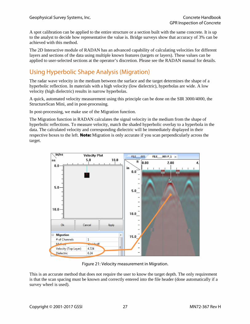
Using Hyperbolic Shape Analysis (Migration) The radar wave velocity in the medium between the surface and the target determines the shape of a hyperbolic reflection. In materials with a high velocity (low dielectric), hyperbolas are wide. A low velocity (high dielectric) results in narrow hyperbolas.

A quick, automated velocity measurement using this principle can be done on the SIR 3000/4000, the StructureScan Mini, and in post-processing.

In post-processing, we make use of the Migration function.

The Migration function in RADAN calculates the signal velocity in the medium from the shape of hyperbolic reflections. To measure velocity, match the shaded hyperbolic overlay to a hyperbola in the data. The calculated velocity and corresponding dielectric will be immediately displayed in their respective boxes to the left. Note: Migration is only accurate if you scan perpendicularly across the target.

Figure 21: Velocity measurement in Migration.

This is an accurate method that does not require the user to know the target depth. The only requirement is that the scan spacing must be known and correctly entered into the file header (done automatically if a survey wheel is used).



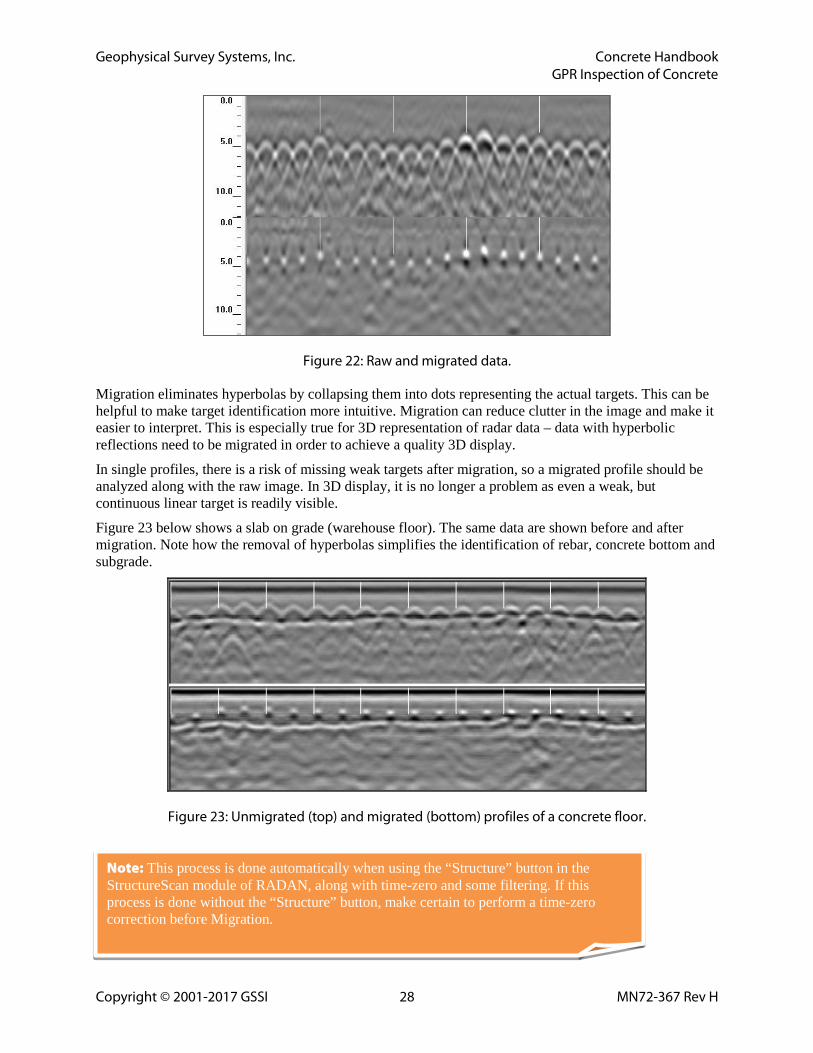
Figure 22: Raw and migrated data.

Migration eliminates hyperbolas by collapsing them into dots representing the actual targets. This can be helpful to make target identification more intuitive. Migration can reduce clutter in the image and make it easier to interpret. This is especially true for 3D representation of radar data – data with hyperbolic reflections need to be migrated in order to achieve a quality 3D display.

In single profiles, there is a risk of missing weak targets after migration, so a migrated profile should be analyzed along with the raw image. In 3D display, it is no longer a problem as even a weak, but continuous linear target is readily visible.

Figure 23 below shows a slab on grade (warehouse floor). The same data are shown before and after migration. Note how the removal of hyperbolas simplifies the identification of rebar, concrete bottom and subgrade.

Figure 23: Unmigrated (top) and migrated (bottom) profiles of a concrete floor.

Note: This process is done automatically when using the “Structure” button in the StructureScan module of RADAN, along with time-zero and some filtering. If this process is done without the “Structure” button, make certain to perform a time-zero correction before Migration.



In the SIR 3000, Migration is not performed as a visual enhancement. Rather, it is performed as a hyperbolic shape analysis process in order to better determine a material’s dielectric constant. This process is known as the “Test Dielectric” process in the SIR 3000 set-up screen. Please see the SIR 3000 manual for details.

In the SIR 4000, Migration is performed as both a visual enhancement as well as a process in order to better determine a material’s dielectric constant. This process is known as “Focus On/Off” in the

SIR 4000 collect screen. Please see the SIR 4000 manual for details.

In the StructureScan Mini, Migration is performed as both a visual enhancement as well as a process in order to better determine a material’s dielectric constant.

The visual enhancement exists in the Collect sub-menu under “Auto-Target”. If the user sets “Auto-Target” to “Focus”, the data will appear normally on the top half of the screen and focused into a point on the bottom half.

In order to better determine a material’s dielectric constant, the user will take advantage of a feature in playback mode called “Auto Depth”. Please refer to the StructureScan Mini Quick-Start Guide for details.

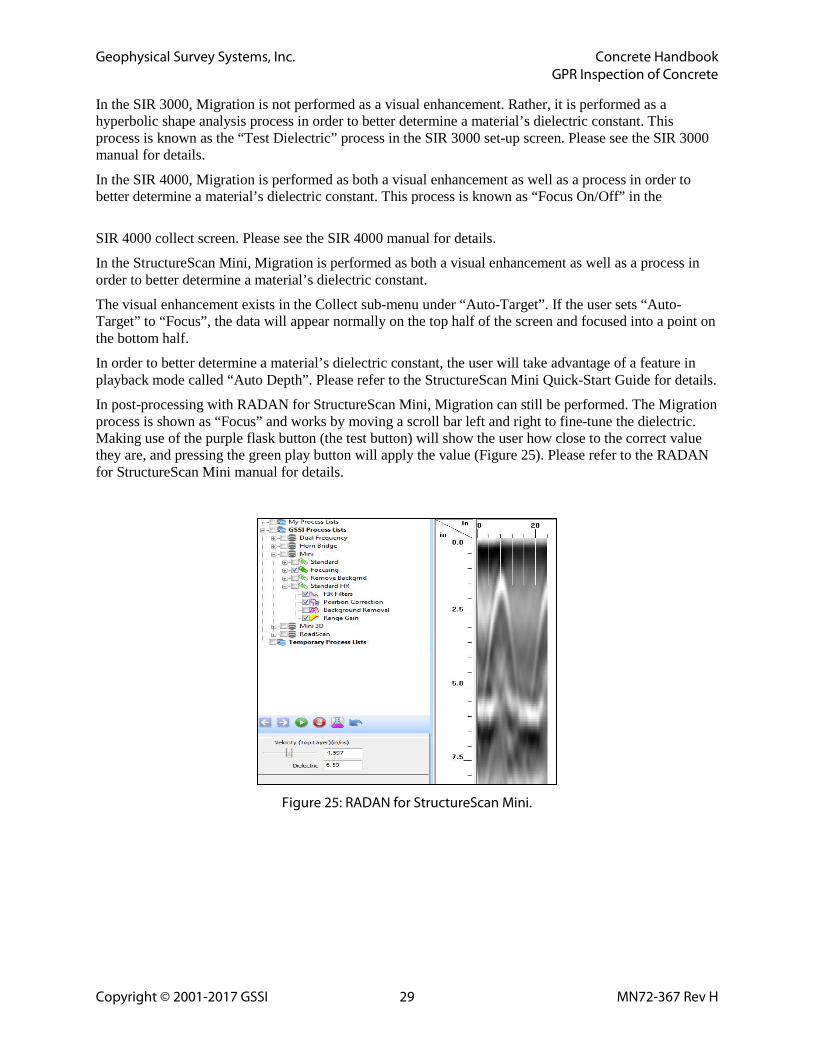
In post-processing with RADAN for StructureScan Mini, Migration can still be performed. The Migration process is shown as “Focus” and works by moving a scroll bar left and right to fine-tune the dielectric. Making use of the purple flask button (the test button) will show the user how close to the correct value they are, and pressing the green play button will apply the value (Figure 25). Please refer to the RADAN for StructureScan Mini manual for details.

Figure 25: RADAN for StructureScan Mini.



Chapter 3: Depth and Position Measurement This section summarizes the above issues and is a step-by-step guide to the actual mapping procedure. The term “mapping” refers to the determination of target position and depth in radar data. Several approaches are to be considered:

• Field measurement using the system screen or a paper printout;

• Manual measurement using post-processing software (RADAN);

• Automated measurement using specialized post-processing software (StructureScan Module).

On sites where continuous mapping of structures with tens or hundreds of reinforcing bars is required, it is strongly recommended to use post-processing software.

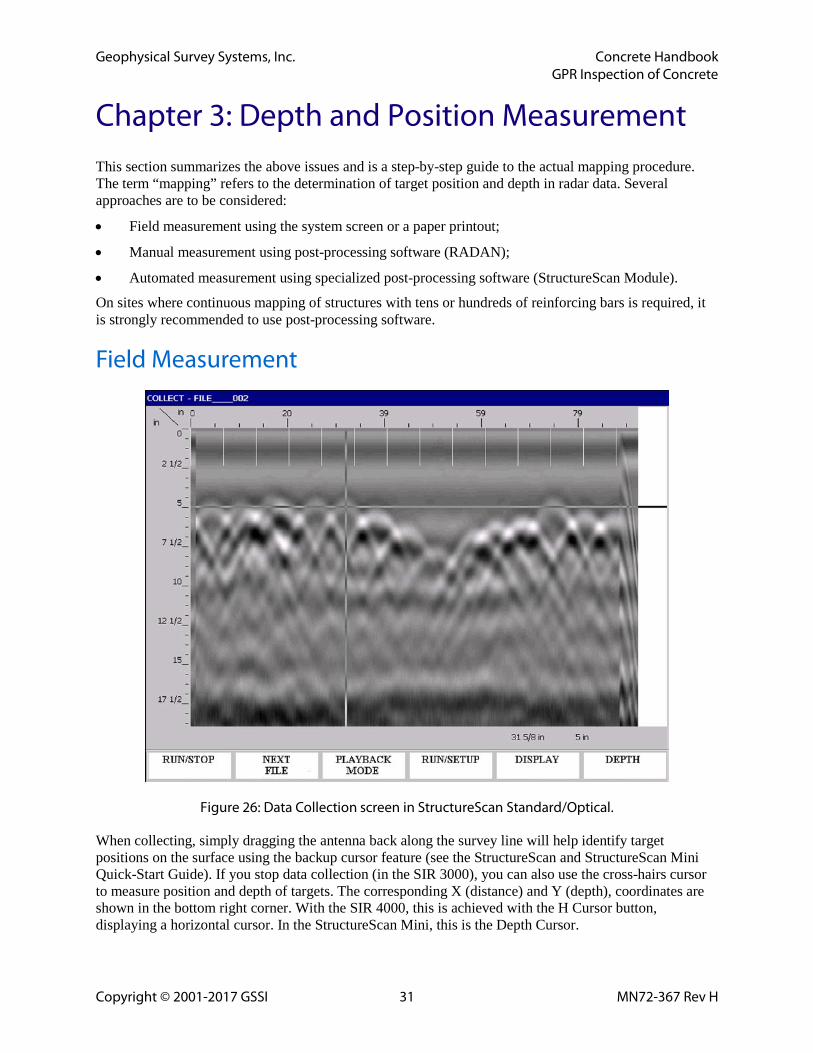
Field Measurement

Figure 26: Data Collection screen in StructureScan Standard/Optical.

When collecting, simply dragging the antenna back along the survey line will help identify target positions on the surface using the backup cursor feature (see the StructureScan and StructureScan Mini Quick-Start Guide). If you stop data collection (in the SIR 3000), you can also use the cross-hairs cursor to measure position and depth of targets. The corresponding X (distance) and Y (depth), coordinates are shown in the bottom right corner. With the SIR 4000, this is achieved with the H Cursor button, displaying a horizontal cursor. In the StructureScan Mini, this is the Depth Cursor.



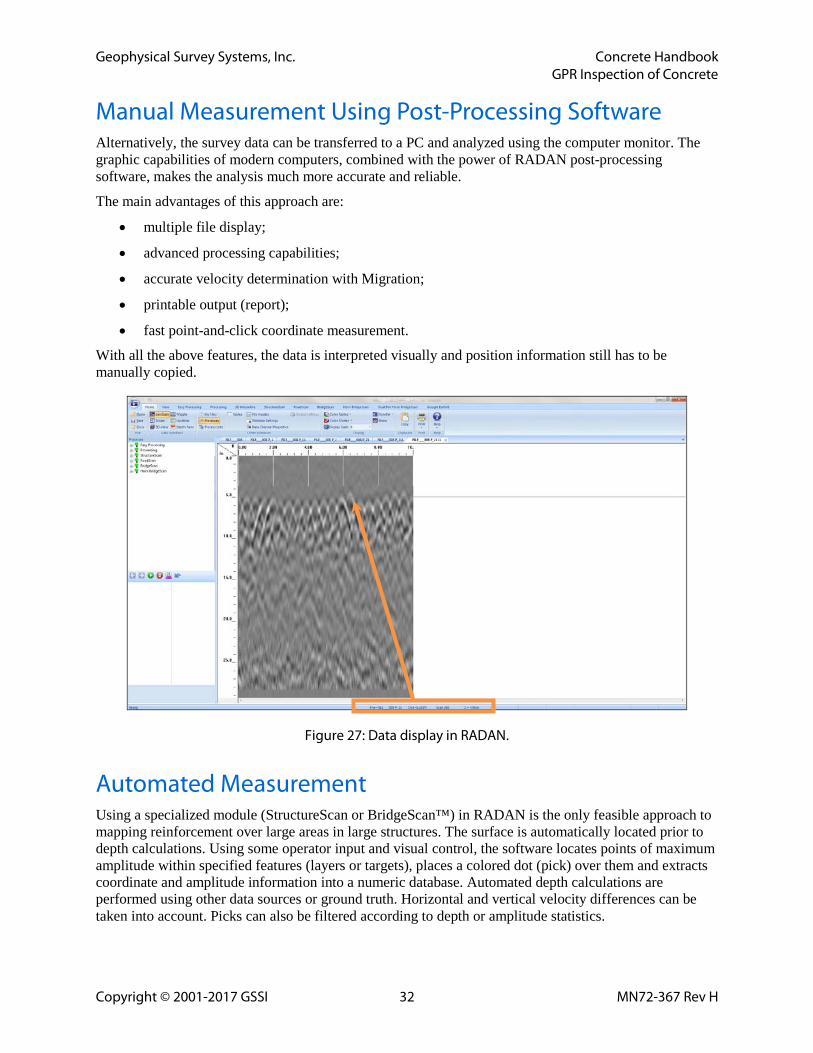
Manual Measurement Using Post-Processing Software Alternatively, the survey data can be transferred to a PC and analyzed using the computer monitor. The graphic capabilities of modern computers, combined with the power of RADAN post-processing software, makes the analysis much more accurate and reliable.

The main advantages of this approach are:

• multiple file display;

• advanced processing capabilities;

• accurate velocity determination with Migration;

• printable output (report);

• fast point-and-click coordinate measurement.

With all the above features, the data is interpreted visually and position information still has to be manually copied.

Figure 27: Data display in RADAN.

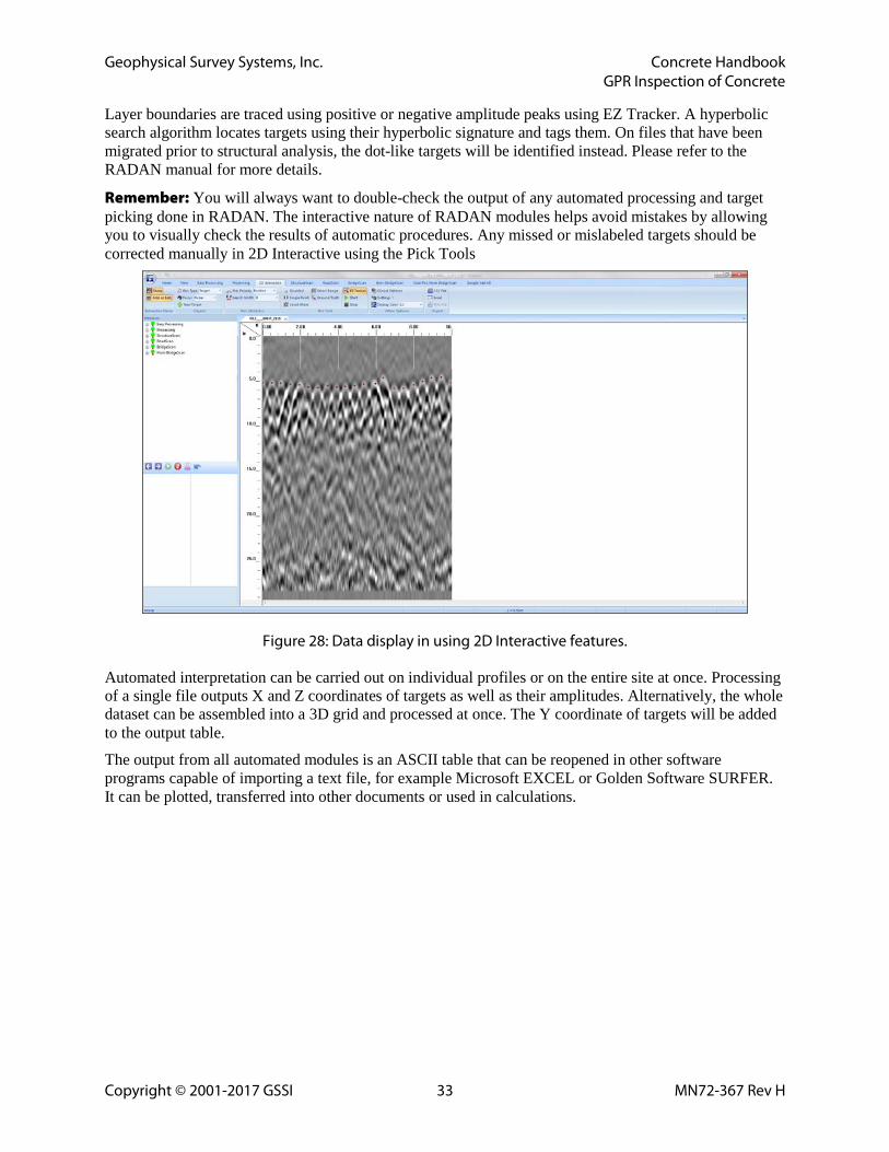
Automated Measurement Using a specialized module (StructureScan or BridgeScan™) in RADAN is the only feasible approach to mapping reinforcement over large areas in large structures. The surface is automatically located prior to depth calculations. Using some operator input and visual control, the software locates points of maximum amplitude within specified features (layers or targets), places a colored dot (pick) over them and extracts coordinate and amplitude information into a numeric database. Automated depth calculations are performed using other data sources or ground truth. Horizontal and vertical velocity differences can be taken into account. Picks can also be filtered according to depth or amplitude statistics.



Layer boundaries are traced using positive or negative amplitude peaks using EZ Tracker. A hyperbolic search algorithm locates targets using their hyperbolic signature and tags them. On files that have been migrated prior to structural analysis, the dot-like targets will be identified instead. Please refer to the RADAN manual for more details.

Remember: You will always want to double-check the output of any automated processing and target picking done in RADAN. The interactive nature of RADAN modules helps avoid mistakes by allowing you to visually check the results of automatic procedures. Any missed or mislabeled targets should be corrected manually in 2D Interactive using the Pick Tools

Figure 28: Data display in using 2D Interactive features.

Automated interpretation can be carried out on individual profiles or on the entire site at once. Processing of a single file outputs X and Z coordinates of targets as well as their amplitudes. Alternatively, the whole dataset can be assembled into a 3D grid and processed at once. The Y coordinate of targets will be added to the output table.

The output from all automated modules is an ASCII table that can be reopened in other software programs capable of importing a text file, for example Microsoft EXCEL or Golden Software SURFER. It can be plotted, transferred into other documents or used in calculations.



Chapter 4: 3D Display of Radar Data 3D display of radar data is one of the most important innovations in GPR. It greatly simplifies data interpretation and allows one to identify targets with confidence. 3D viewing is more intuitive than single-line analysis and allows the identification of subtle features that are easily missed in single profiles. Identification of targets is simplified because their true shape and spatial relationship to other objects becomes visible.

It must be understood that we’re talking about “simulated 3D”. A three-dimensional image is created by simultaneously displaying several “conventional” radar lines parallel to each other. Interpolation between these lines gives the impression of a continuous image of the entire survey area.

3D display is most efficient for linear targets. The human eye easily recognizes linear features, even very weak or intermittent. A plan view is the most practical way of looking at 3D datasets. Cables, conduits, etc. can be quickly mapped from a plan view.

RADAN offers two different approaches to 3D imaging, Depth Slices and using the 3D-View data window in Standard Processing or RADAN for StructureScan Mini.

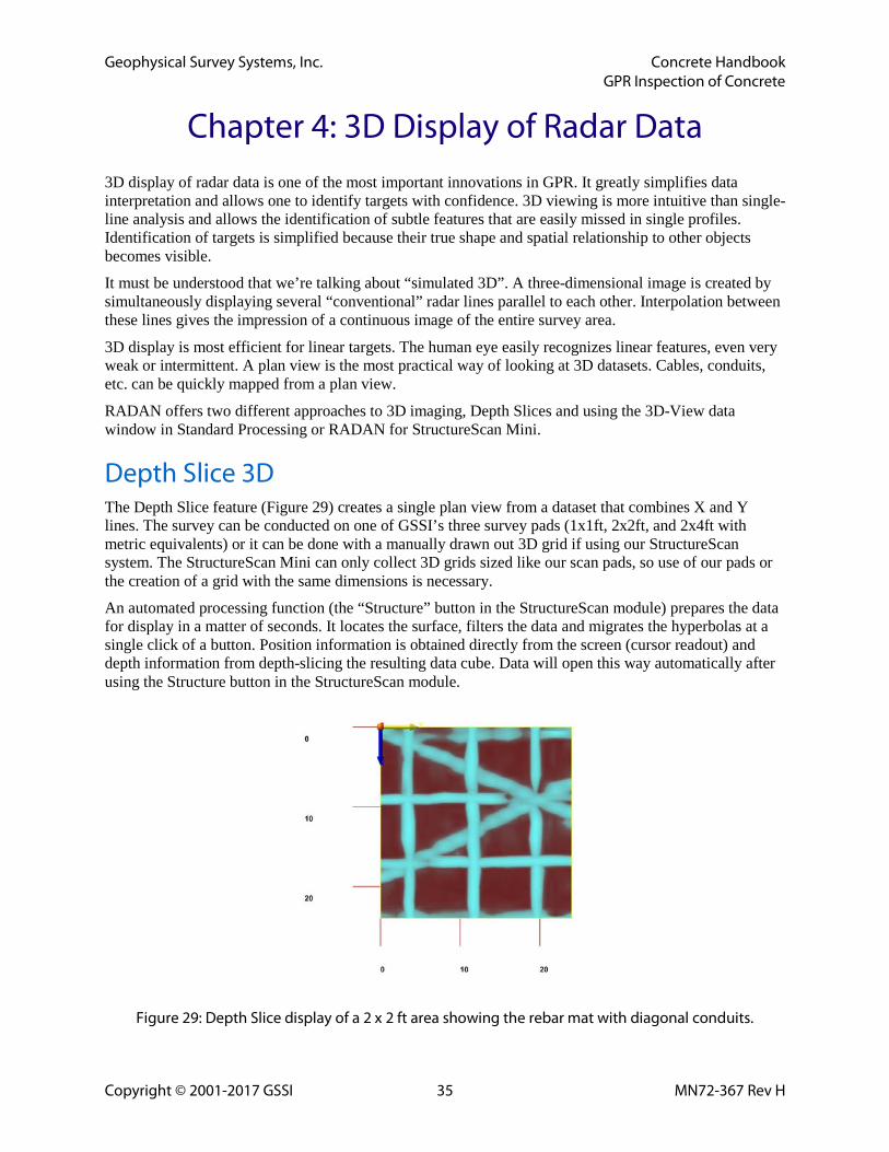
Depth Slice 3D The Depth Slice feature (Figure 29) creates a single plan view from a dataset that combines X and Y lines. The survey can be conducted on one of GSSI’s three survey pads (1x1ft, 2x2ft, and 2x4ft with metric equivalents) or it can be done with a manually drawn out 3D grid if using our StructureScan system. The StructureScan Mini can only collect 3D grids sized like our scan pads, so use of our pads or the creation of a grid with the same dimensions is necessary.

An automated processing function (the “Structure” button in the StructureScan module) prepares the data for display in a matter of seconds. It locates the surface, filters the data and migrates the hyperbolas at a single click of a button. Position information is obtained directly from the screen (cursor readout) and depth information from depth-slicing the resulting data cube. Data will open this way automatically after using the Structure button in the StructureScan module.

Figure 29: Depth Slice display of a 2 x 2 ft area showing the rebar mat with diagonal conduits.



Note: 3D views are an excellent tool for feature identification. It is best to use them in combination with the regular vertical profiles (the 2D transects) comprising the 3D view. Individual profiles contain information about

3D-View and Super 3D

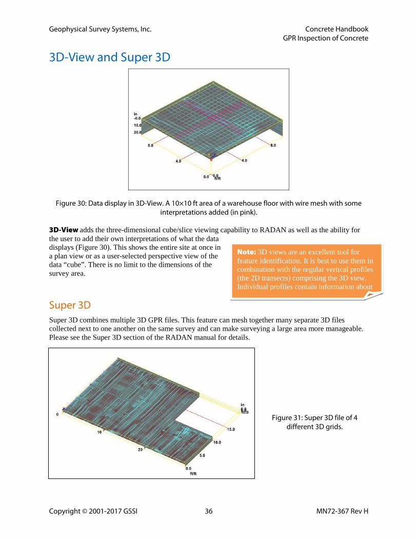
Figure 30: Data display in 3D-View. A 10×10 ft area of a warehouse floor with wire mesh with some interpretations added (in pink).

3D-View adds the three-dimensional cube/slice viewing capability to RADAN as well as the ability for the user to add their own interpretations of what the data displays (Figure 30). This shows the entire site at once in a plan view or as a user-selected perspective view of the data “cube”. There is no limit to the dimensions of the survey area.

Super 3D Super 3D combines multiple 3D GPR files. This feature can mesh together many separate 3D files collected next to one another on the same survey and can make surveying a large area more manageable. Please see the Super 3D section of the RADAN manual for details.

Figure 31: Super 3D file of 4 different 3D grids.

gpr inspection of concrete - gssi inc. · geophysical survey systems, inc. concrete handbook gpr...

Documents