goback - kit - fakultät für mathematikrieder/media/obergurgl_slides.pdf · c andreas rieder –...
TRANSCRIPT

GoBack
c©Andreas Rieder – Workshop Hybrid Imaging, Obergurgl, January 2008 – 1 / 24
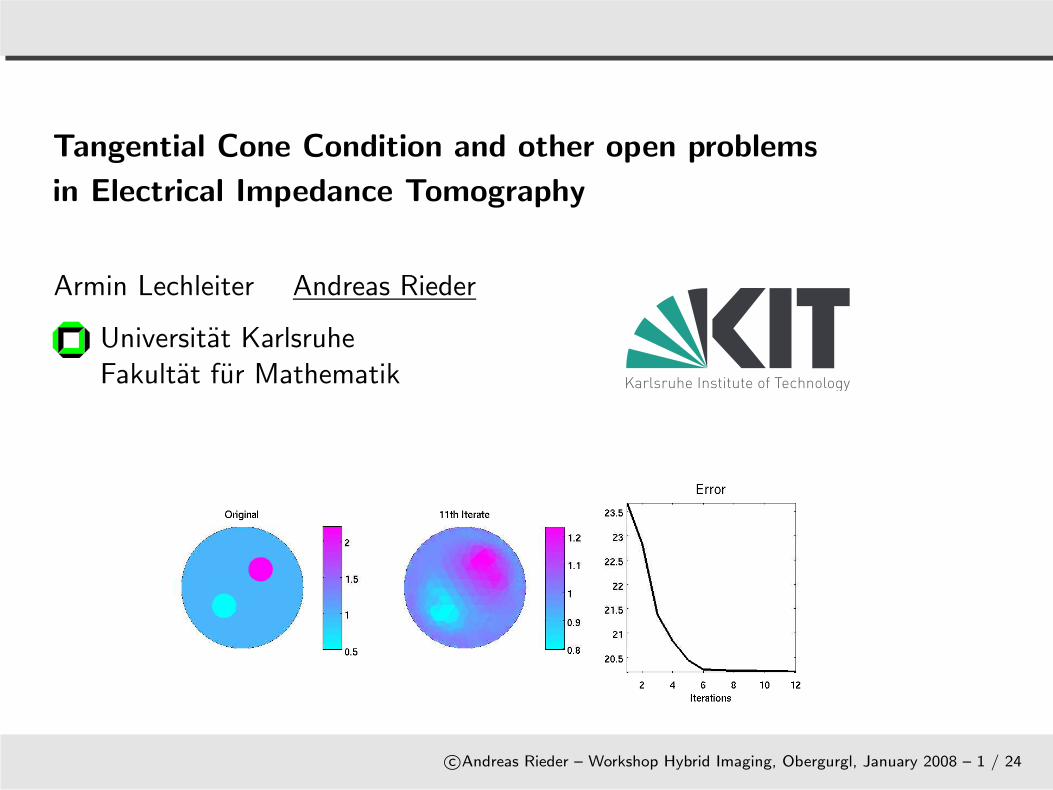
Tangential Cone Condition and other open problems
in Electrical Impedance Tomography
Armin Lechleiter Andreas Rieder
Universitat KarlsruheFakultat fur Mathematik
Overview
The Tangential ConeCondition (TCC)
EIT: ContinuousModel
EIT: CompleteElectrode Model
Conclusion
c©Andreas Rieder – Workshop Hybrid Imaging, Obergurgl, January 2008 – 2 / 24
The Tangential Cone Condition (TCC)
EIT: Continuous Model
EIT: Complete Electrode Model
Conclusion
The Tangential Cone Condition (TCC)
.
The TangentialCone Condition(TCC)
EIT: ContinuousModel
EIT: CompleteElectrode Model
Conclusion
c©Andreas Rieder – Workshop Hybrid Imaging, Obergurgl, January 2008 – 3 / 24
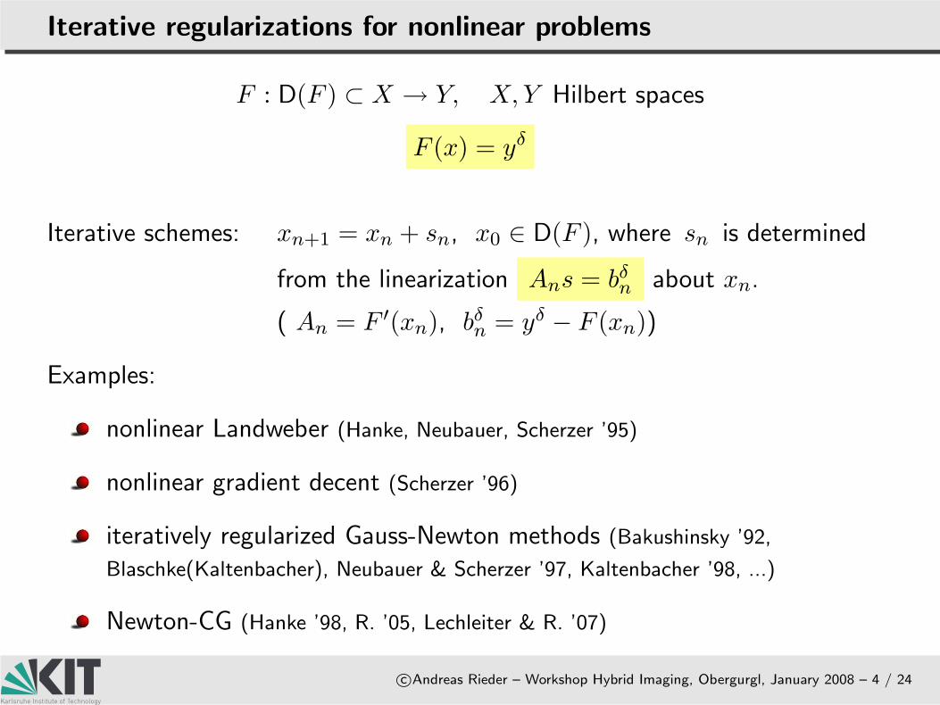
Iterative regularizations for nonlinear problems
c©Andreas Rieder – Workshop Hybrid Imaging, Obergurgl, January 2008 – 4 / 24
F : D(F ) ⊂ X → Y, X, Y Hilbert spaces
F (x) = yδ
Iterative schemes: xn+1 = xn + sn, x0 ∈ D(F ), where sn is determined
from the linearization Ans = bδn about xn.
( An = F ′(xn), bδn = yδ − F (xn))
Examples:
nonlinear Landweber (Hanke, Neubauer, Scherzer ’95)
nonlinear gradient decent (Scherzer ’96)
iteratively regularized Gauss-Newton methods (Bakushinsky ’92,
Blaschke(Kaltenbacher), Neubauer & Scherzer ’97, Kaltenbacher ’98, ...)
Newton-CG (Hanke ’98, R. ’05, Lechleiter & R. ’07)
The need for the tangential cone condition
c©Andreas Rieder – Workshop Hybrid Imaging, Obergurgl, January 2008 – 5 / 24
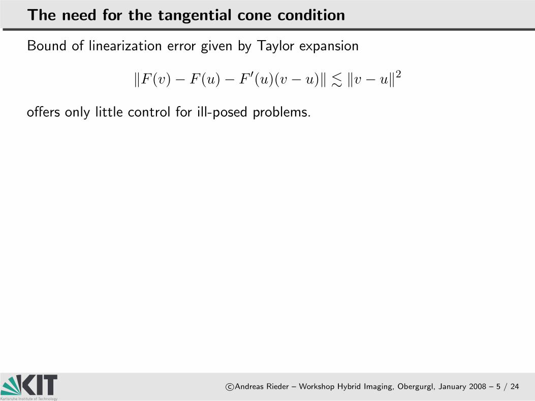
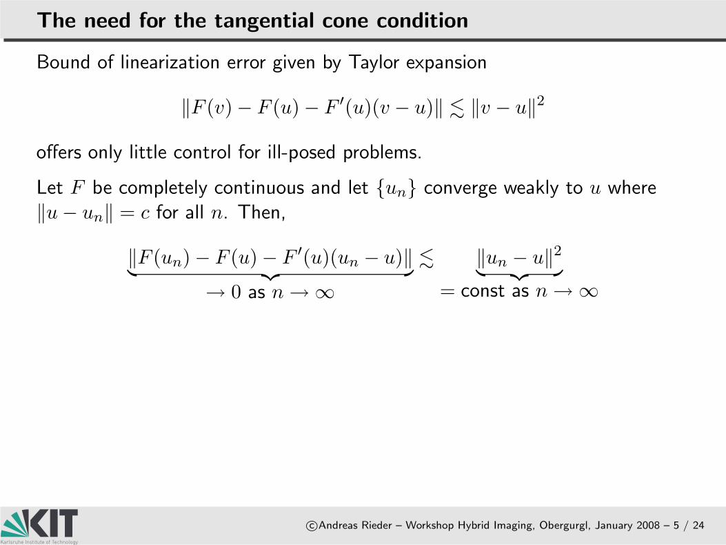
Bound of linearization error given by Taylor expansion
‖F (v) − F (u) − F ′(u)(v − u)‖ . ‖v − u‖2
offers only little control for ill-posed problems.
The need for the tangential cone condition
c©Andreas Rieder – Workshop Hybrid Imaging, Obergurgl, January 2008 – 5 / 24
Bound of linearization error given by Taylor expansion
‖F (v) − F (u) − F ′(u)(v − u)‖ . ‖v − u‖2
offers only little control for ill-posed problems.
Let F be completely continuous and let un converge weakly to u where‖u − un‖ = c for all n. Then,
‖F (un) − F (u) − F ′(u)(un − u)‖︸ ︷︷ ︸
→ 0 as n → ∞
. ‖un − u‖2
︸ ︷︷ ︸
= const as n → ∞
Tangential cone condition (TCC)
c©Andreas Rieder – Workshop Hybrid Imaging, Obergurgl, January 2008 – 6 / 24
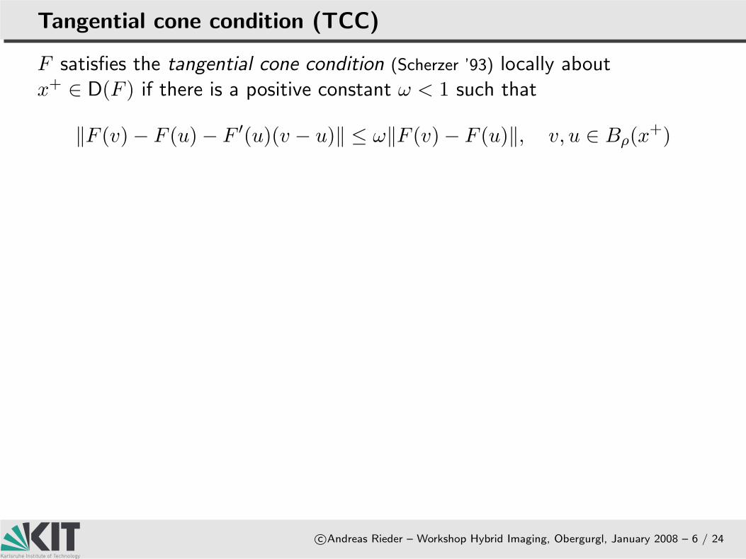
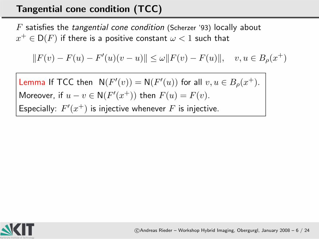
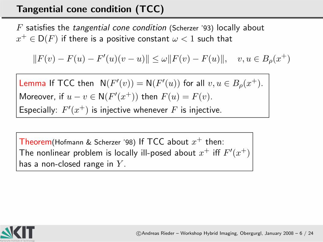
F satisfies the tangential cone condition (Scherzer ’93) locally aboutx+ ∈ D(F ) if there is a positive constant ω < 1 such that
‖F (v) − F (u) − F ′(u)(v − u)‖ ≤ ω‖F (v) − F (u)‖, v, u ∈ Bρ(x+)
Tangential cone condition (TCC)
c©Andreas Rieder – Workshop Hybrid Imaging, Obergurgl, January 2008 – 6 / 24
F satisfies the tangential cone condition (Scherzer ’93) locally aboutx+ ∈ D(F ) if there is a positive constant ω < 1 such that
‖F (v) − F (u) − F ′(u)(v − u)‖ ≤ ω‖F (v) − F (u)‖, v, u ∈ Bρ(x+)
Lemma If TCC then N(F ′(v)) = N(F ′(u)) for all v, u ∈ Bρ(x+).
Moreover, if u − v ∈ N(F ′(x+)) then F (u) = F (v).
Especially: F ′(x+) is injective whenever F is injective.
Theorem(Hofmann & Scherzer ’98) If TCC about x+ then:The nonlinear problem is locally ill-posed about x+ iff F ′(x+)has a non-closed range in Y .
EIT: Continuous Model
The Tangential ConeCondition (TCC)
.EIT: ContinuousModel
EIT: CompleteElectrode Model
Conclusion
c©Andreas Rieder – Workshop Hybrid Imaging, Obergurgl, January 2008 – 7 / 24
Governing equation
c©Andreas Rieder – Workshop Hybrid Imaging, Obergurgl, January 2008 – 8 / 24
σ(x)
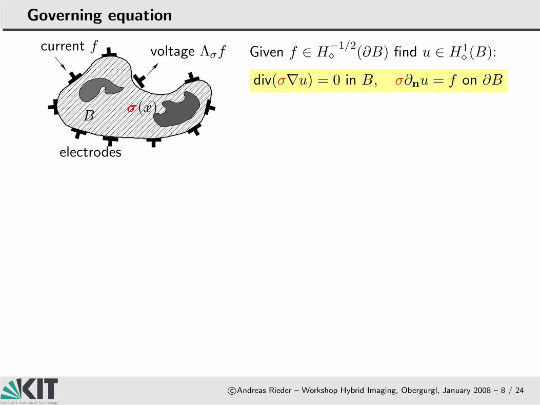
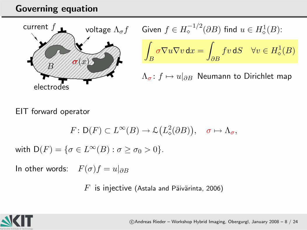
current f voltage Λσf
electrodes
B
Given f ∈ H−1/2 (∂B) find u ∈ H1
(B):
div(σ∇u) = 0 in B, σ∂nu = f on ∂B
Governing equation
c©Andreas Rieder – Workshop Hybrid Imaging, Obergurgl, January 2008 – 8 / 24
σ(x)
current f voltage Λσf
electrodes
B
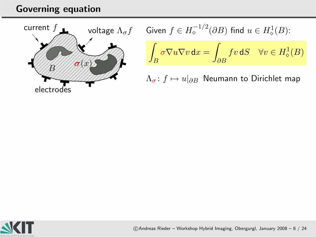
Given f ∈ H−1/2 (∂B) find u ∈ H1
(B):
∫
Bσ∇u∇v dx =
∫
∂Bfv dS ∀v ∈ H1
(B)
Λσ : f 7→ u|∂B Neumann to Dirichlet map
Governing equation
c©Andreas Rieder – Workshop Hybrid Imaging, Obergurgl, January 2008 – 8 / 24
σ(x)
current f voltage Λσf
electrodes
B
Given f ∈ H−1/2 (∂B) find u ∈ H1
(B):
∫
Bσ∇u∇v dx =
∫
∂Bfv dS ∀v ∈ H1
(B)
Λσ : f 7→ u|∂B Neumann to Dirichlet map
EIT forward operator
F : D(F ) ⊂ L∞(B) → L(L2(∂B)
), σ 7→ Λσ,
with D(F ) = σ ∈ L∞(B) : σ ≥ σ0 > 0.
In other words: F (σ)f = u|∂B
F is injective (Astala and Paivarinta, 2006)
Frechet differentiability of EIT operator
c©Andreas Rieder – Workshop Hybrid Imaging, Obergurgl, January 2008 – 9 / 24
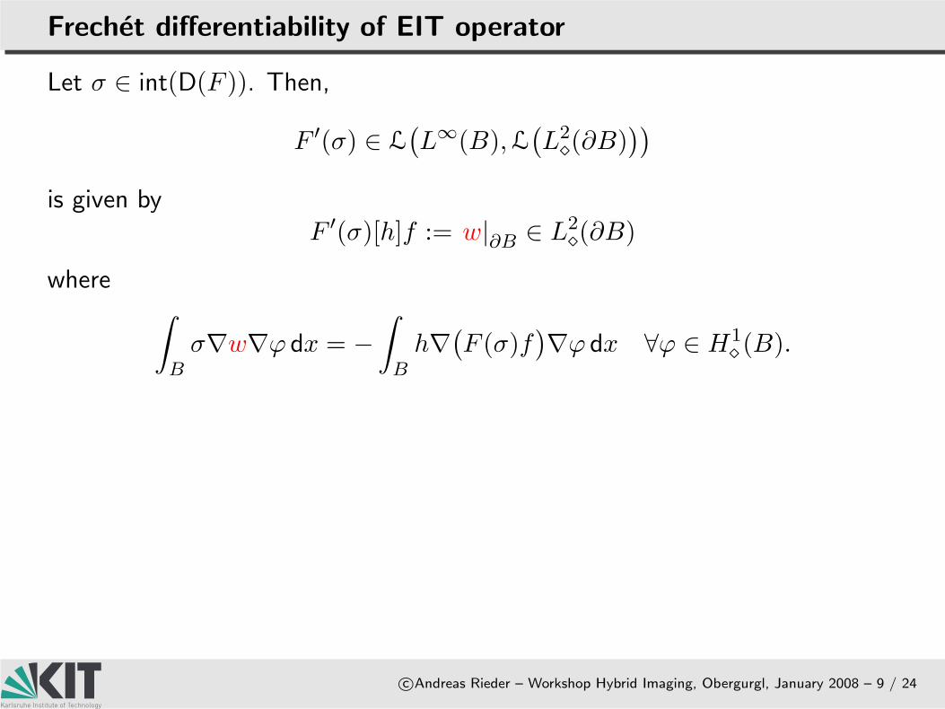
Let σ ∈ int(D(F )). Then,
F ′(σ) ∈ L(L∞(B), L
(L2(∂B)
))
is given byF ′(σ)[h]f := w|∂B ∈ L2
(∂B)
where∫
Bσ∇w∇ϕ dx = −
∫
Bh∇
(F (σ)f
)∇ϕ dx ∀ϕ ∈ H1
(B).
On the injectivity of F′(σ)
c©Andreas Rieder – Workshop Hybrid Imaging, Obergurgl, January 2008 – 10 / 24
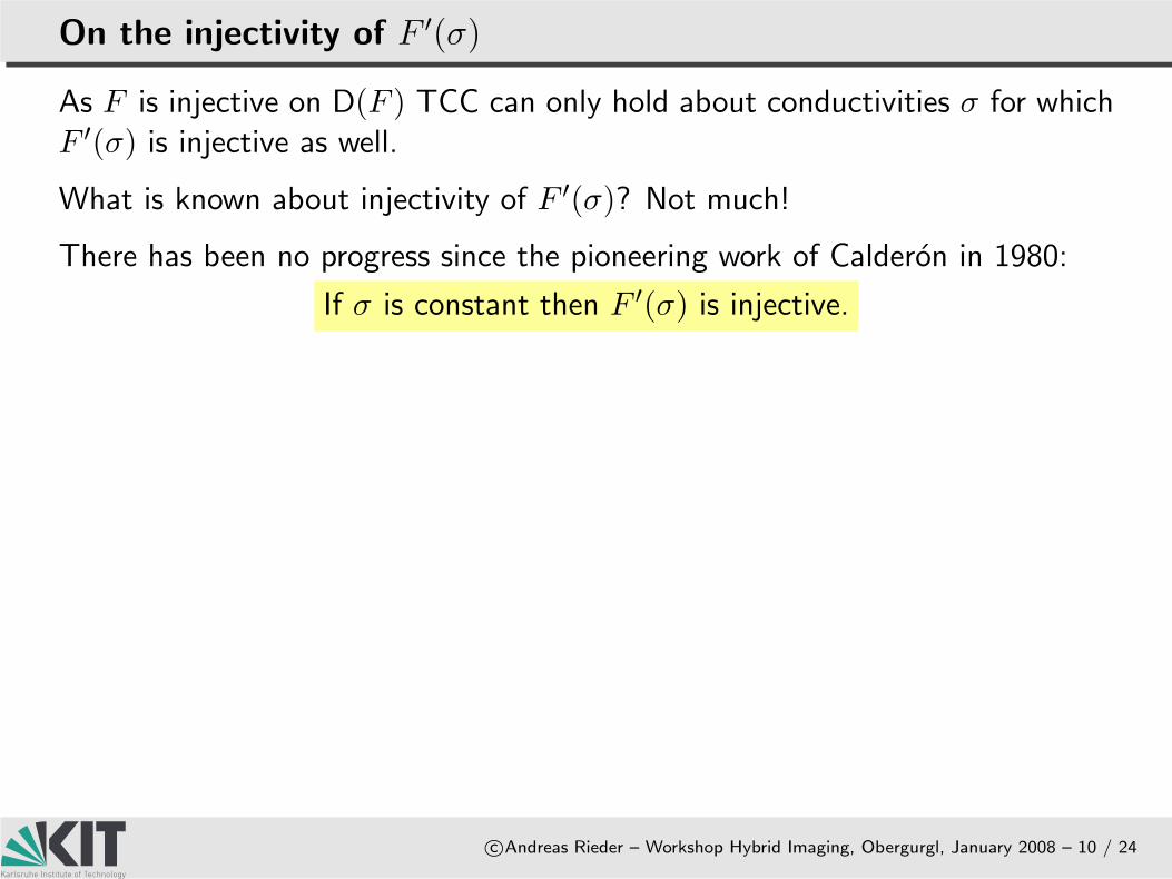
As F is injective on D(F ) TCC can only hold about conductivities σ for whichF ′(σ) is injective as well.
What is known about injectivity of F ′(σ)?
On the injectivity of F′(σ)
c©Andreas Rieder – Workshop Hybrid Imaging, Obergurgl, January 2008 – 10 / 24
As F is injective on D(F ) TCC can only hold about conductivities σ for whichF ′(σ) is injective as well.
What is known about injectivity of F ′(σ)? Not much!
On the injectivity of F′(σ)
c©Andreas Rieder – Workshop Hybrid Imaging, Obergurgl, January 2008 – 10 / 24
As F is injective on D(F ) TCC can only hold about conductivities σ for whichF ′(σ) is injective as well.
What is known about injectivity of F ′(σ)? Not much!
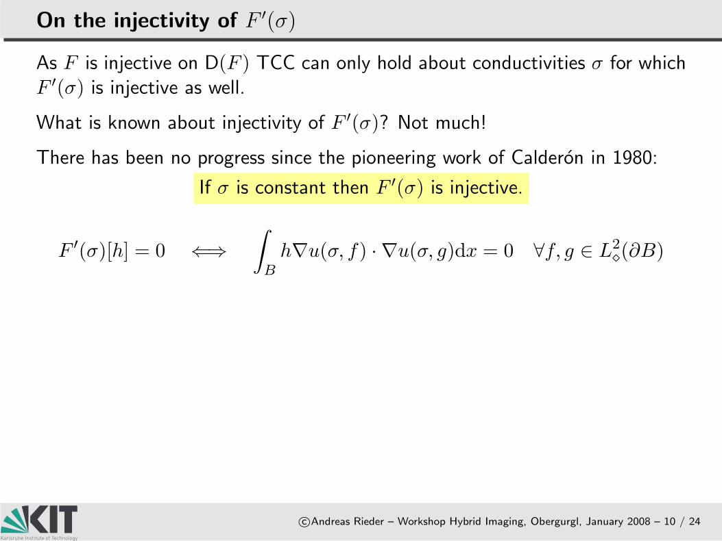
There has been no progress since the pioneering work of Calderon in 1980:
If σ is constant then F ′(σ) is injective.
On the injectivity of F′(σ)
c©Andreas Rieder – Workshop Hybrid Imaging, Obergurgl, January 2008 – 10 / 24
As F is injective on D(F ) TCC can only hold about conductivities σ for whichF ′(σ) is injective as well.
What is known about injectivity of F ′(σ)? Not much!
There has been no progress since the pioneering work of Calderon in 1980:
If σ is constant then F ′(σ) is injective.
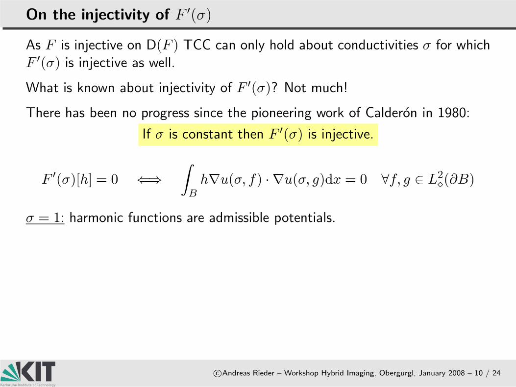
F ′(σ)[h] = 0 ⇐⇒
∫
Bh∇u(σ, f) · ∇u(σ, g)dx = 0 ∀f, g ∈ L2
(∂B)
On the injectivity of F′(σ)
c©Andreas Rieder – Workshop Hybrid Imaging, Obergurgl, January 2008 – 10 / 24
As F is injective on D(F ) TCC can only hold about conductivities σ for whichF ′(σ) is injective as well.
What is known about injectivity of F ′(σ)? Not much!
There has been no progress since the pioneering work of Calderon in 1980:
If σ is constant then F ′(σ) is injective.
F ′(σ)[h] = 0 ⇐⇒
∫
Bh∇u(σ, f) · ∇u(σ, g)dx = 0 ∀f, g ∈ L2
(∂B)
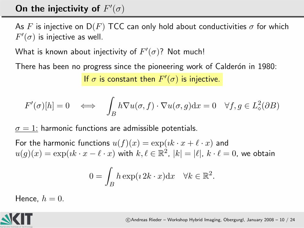
σ = 1: harmonic functions are admissible potentials.
On the injectivity of F′(σ)
c©Andreas Rieder – Workshop Hybrid Imaging, Obergurgl, January 2008 – 10 / 24
As F is injective on D(F ) TCC can only hold about conductivities σ for whichF ′(σ) is injective as well.
What is known about injectivity of F ′(σ)? Not much!
There has been no progress since the pioneering work of Calderon in 1980:
If σ is constant then F ′(σ) is injective.
F ′(σ)[h] = 0 ⇐⇒
∫
Bh∇u(σ, f) · ∇u(σ, g)dx = 0 ∀f, g ∈ L2
(∂B)
σ = 1: harmonic functions are admissible potentials.
For the harmonic functions u(f)(x) = exp(ık · x + ` · x) andu(g)(x) = exp(ık · x − ` · x) with k, ` ∈ R
2, |k| = |`|, k · ` = 0, we obtain
0 =
∫
Bh exp(ı 2k · x)dx ∀k ∈ R
2.
Hence, h = 0.
On the injectivity of F′(σ) (continued)
c©Andreas Rieder – Workshop Hybrid Imaging, Obergurgl, January 2008 – 11 / 24
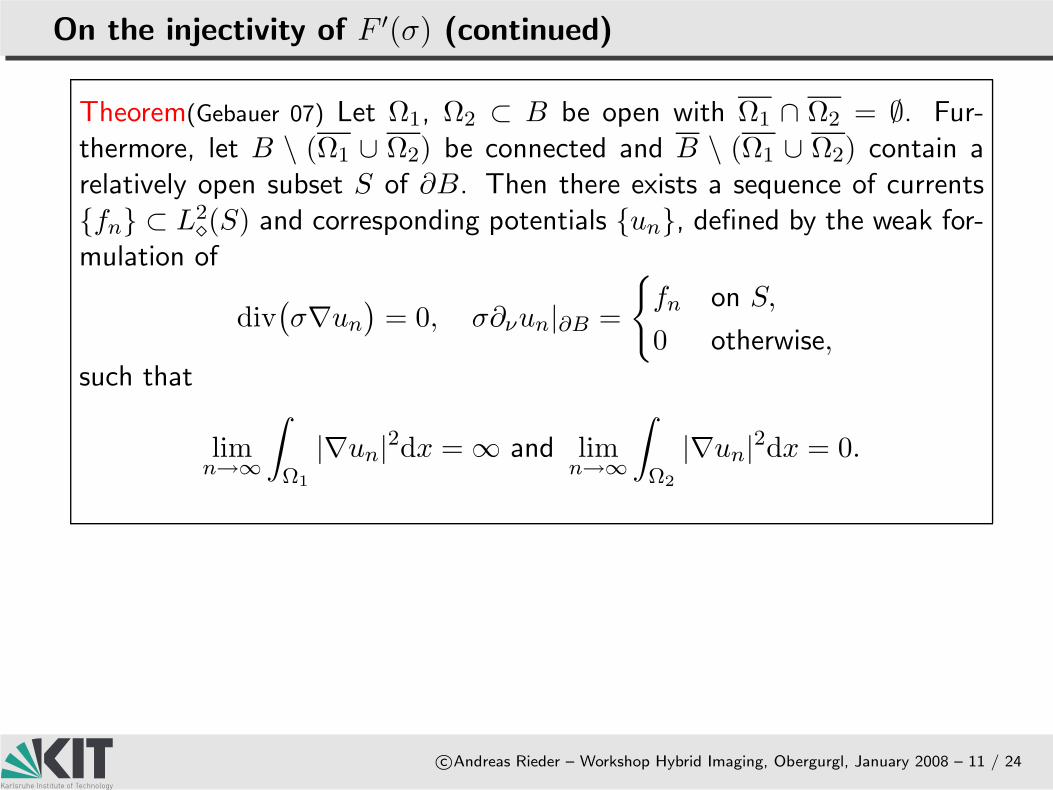
Theorem(Gebauer 07) Let Ω1, Ω2 ⊂ B be open with Ω1 ∩ Ω2 = ∅. Fur-thermore, let B \ (Ω1 ∪ Ω2) be connected and B \ (Ω1 ∪ Ω2) contain arelatively open subset S of ∂B. Then there exists a sequence of currentsfn ⊂ L2
(S) and corresponding potentials un, defined by the weak for-
mulation of
div(σ∇un
)= 0, σ∂νun|∂B =
fn on S,
0 otherwise,such that
limn→∞
∫
Ω1
|∇un|2dx = ∞ and lim
n→∞
∫
Ω2
|∇un|2dx = 0.
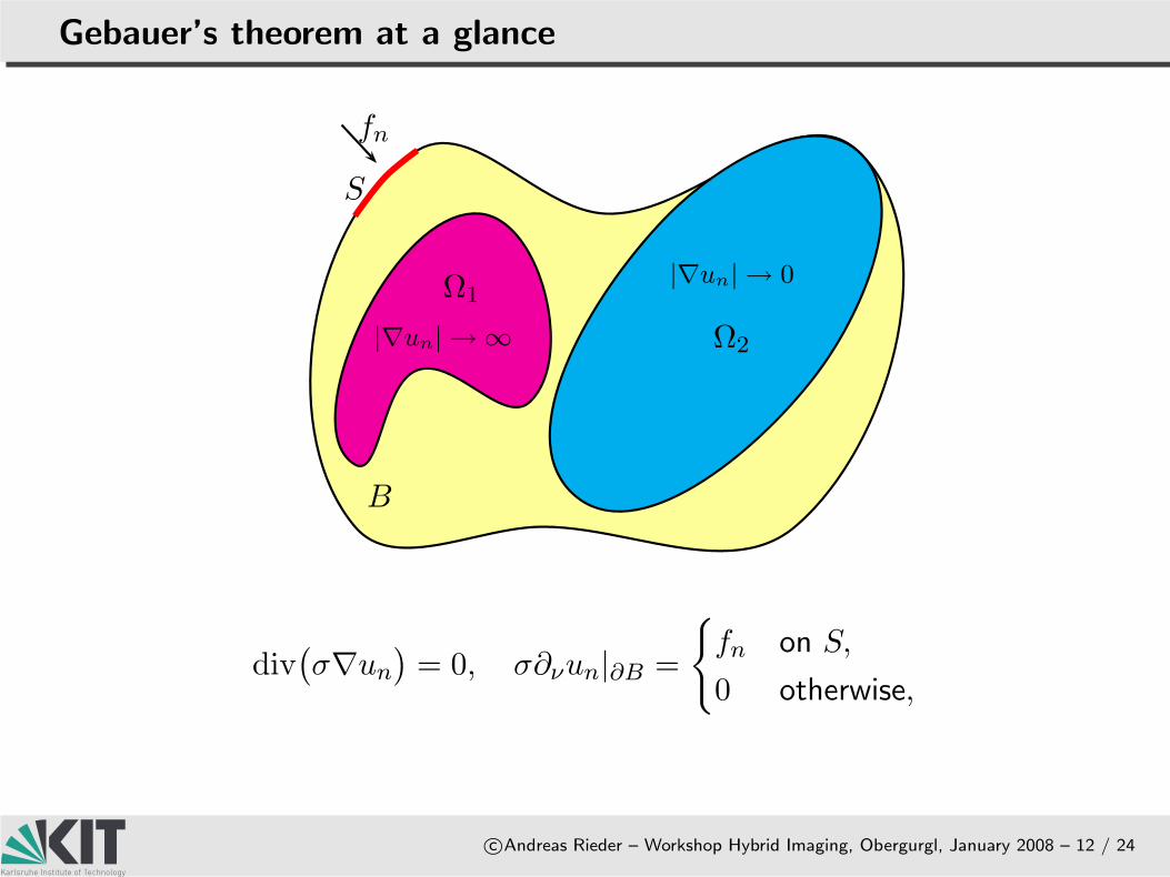
Gebauer’s theorem at a glance
c©Andreas Rieder – Workshop Hybrid Imaging, Obergurgl, January 2008 – 12 / 24
Ω1
Ω2
B
S
fn
|∇un| → ∞
|∇un| → 0
div(σ∇un
)= 0, σ∂νun|∂B =
fn on S,
0 otherwise,
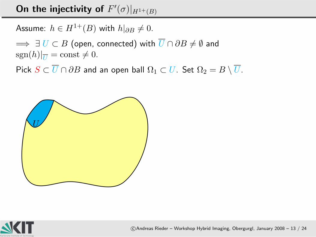
On the injectivity of F′(σ)|H1+(B)
c©Andreas Rieder – Workshop Hybrid Imaging, Obergurgl, January 2008 – 13 / 24
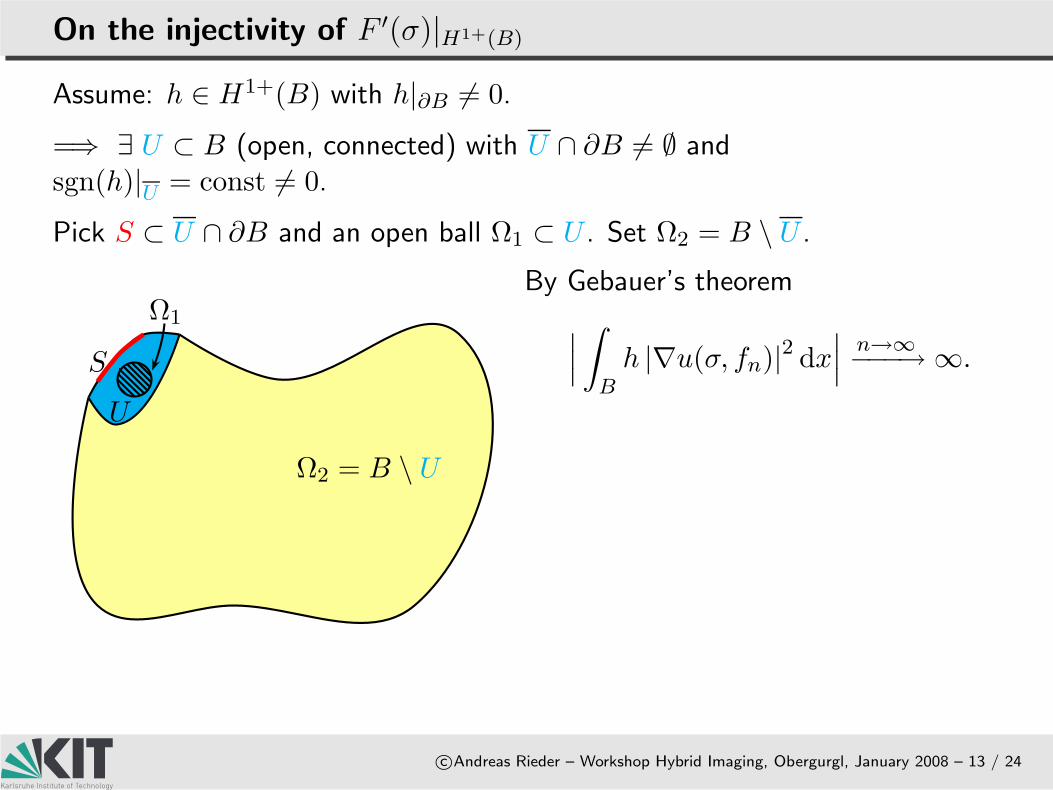
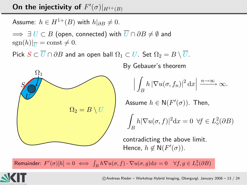
Assume: h ∈ H1+(B) with h|∂B 6= 0.
=⇒ ∃ U ⊂ B (open, connected) with U ∩ ∂B 6= ∅ andsgn(h)|U = const 6= 0.
Pick S ⊂ U ∩ ∂B and an open ball Ω1 ⊂ U . Set Ω2 = B \ U .
U
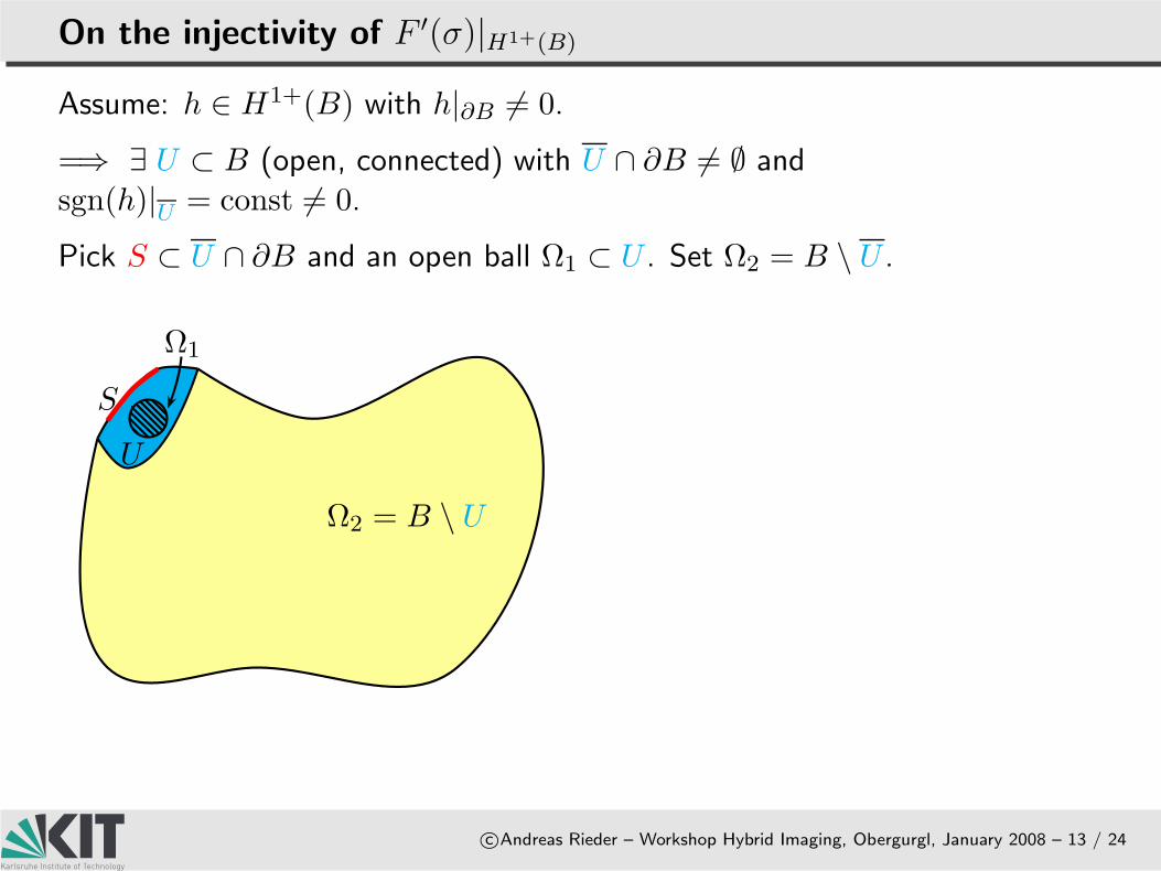
On the injectivity of F′(σ)|H1+(B)
c©Andreas Rieder – Workshop Hybrid Imaging, Obergurgl, January 2008 – 13 / 24
Assume: h ∈ H1+(B) with h|∂B 6= 0.
=⇒ ∃ U ⊂ B (open, connected) with U ∩ ∂B 6= ∅ andsgn(h)|U = const 6= 0.
Pick S ⊂ U ∩ ∂B and an open ball Ω1 ⊂ U . Set Ω2 = B \ U .
Ω1
Ω2 = B \ U
U
S
On the injectivity of F′(σ)|H1+(B)
c©Andreas Rieder – Workshop Hybrid Imaging, Obergurgl, January 2008 – 13 / 24
Assume: h ∈ H1+(B) with h|∂B 6= 0.
=⇒ ∃ U ⊂ B (open, connected) with U ∩ ∂B 6= ∅ andsgn(h)|U = const 6= 0.
Pick S ⊂ U ∩ ∂B and an open ball Ω1 ⊂ U . Set Ω2 = B \ U .
Ω1
Ω2 = B \ U
U
S
By Gebauer’s theorem
∣∣∣
∫
Bh |∇u(σ, fn)|2 dx
∣∣∣
n→∞
−−−→ ∞.
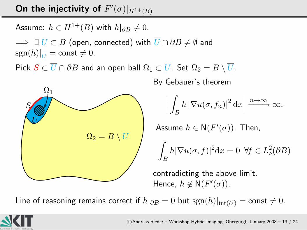
Assume h ∈ N(F ′(σ)). Then,
∫
Bh|∇u(σ, f)|2dx = 0 ∀f ∈ L2
(∂B)
contradicting the above limit.Hence, h 6∈ N(F ′(σ)).
Remainder: F ′(σ)[h] = 0 ⇐⇒∫
Bh∇u(σ, f) · ∇u(σ, g)dx = 0 ∀f, g ∈ L2
(∂B)
On the injectivity of F′(σ)|H1+(B)
c©Andreas Rieder – Workshop Hybrid Imaging, Obergurgl, January 2008 – 13 / 24
Assume: h ∈ H1+(B) with h|∂B 6= 0.
=⇒ ∃ U ⊂ B (open, connected) with U ∩ ∂B 6= ∅ andsgn(h)|U = const 6= 0.
Pick S ⊂ U ∩ ∂B and an open ball Ω1 ⊂ U . Set Ω2 = B \ U .
Ω1
Ω2 = B \ U
U
S
By Gebauer’s theorem
∣∣∣
∫
Bh |∇u(σ, fn)|2 dx
∣∣∣
n→∞
−−−→ ∞.
Assume h ∈ N(F ′(σ)). Then,
∫
Bh|∇u(σ, f)|2dx = 0 ∀f ∈ L2
(∂B)
contradicting the above limit.Hence, h 6∈ N(F ′(σ)).
Line of reasoning remains correct if h|∂B = 0 but sgn(h)|int(U) = const 6= 0.
On the injectivity of F′(σ)|H1+(B) (continued)
c©Andreas Rieder – Workshop Hybrid Imaging, Obergurgl, January 2008 – 14 / 24
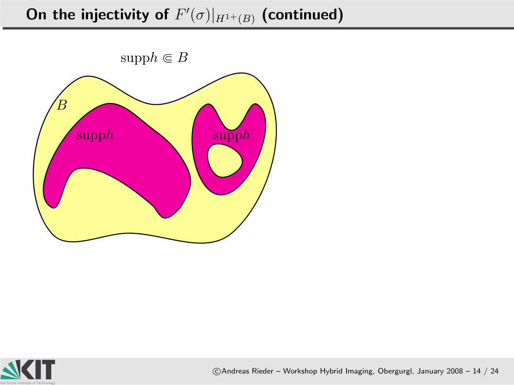
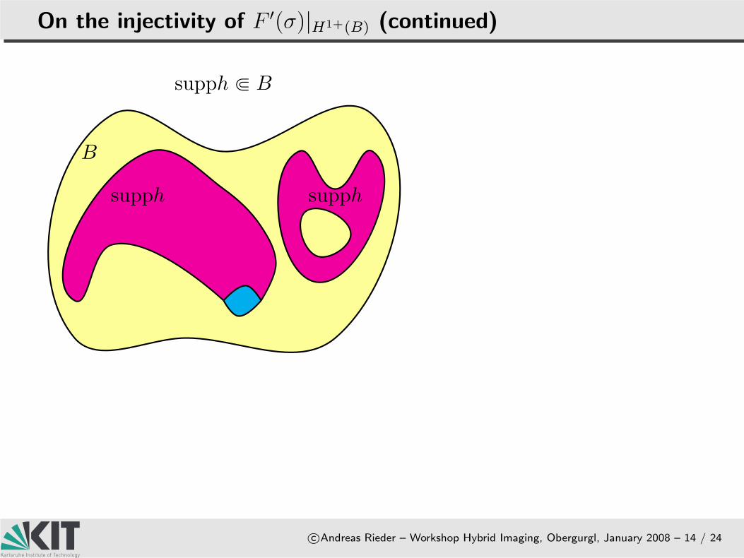
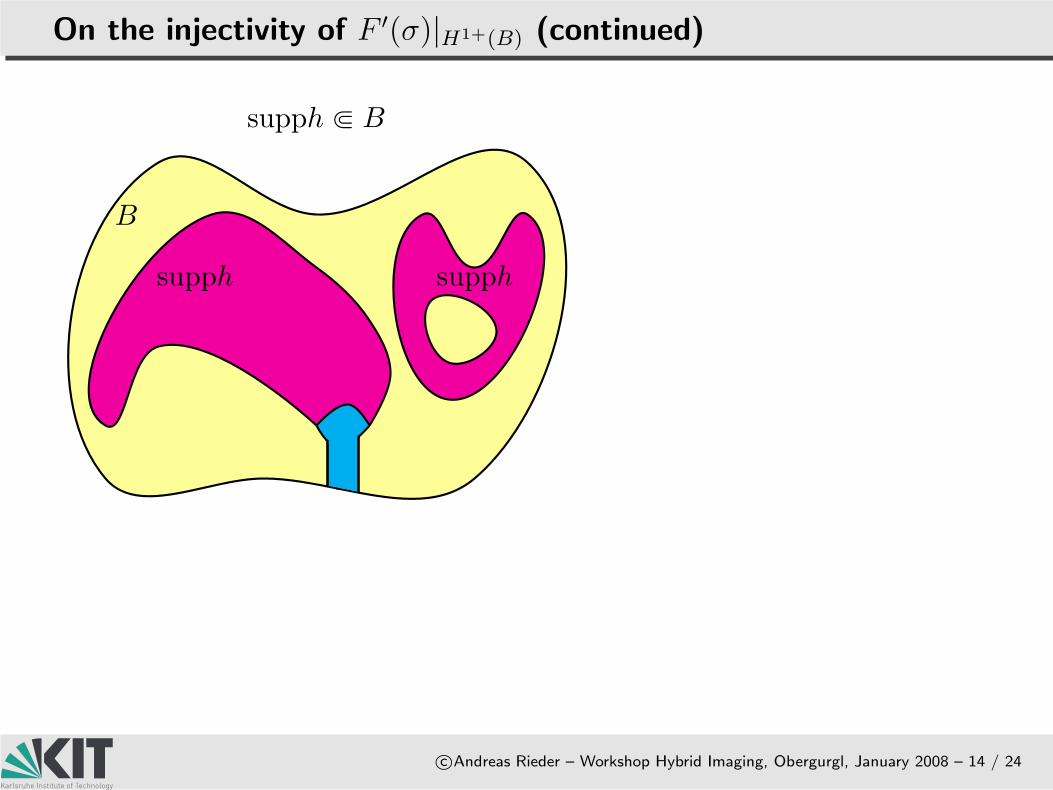
supph supph
B
supph b B
On the injectivity of F′(σ)|H1+(B) (continued)
c©Andreas Rieder – Workshop Hybrid Imaging, Obergurgl, January 2008 – 14 / 24
supph supph
B
supph b B

On the injectivity of F′(σ)|H1+(B) (continued)
c©Andreas Rieder – Workshop Hybrid Imaging, Obergurgl, January 2008 – 14 / 24
supph supph
B
supph b B
On the injectivity of F′(σ)|H1+(B) (continued)
c©Andreas Rieder – Workshop Hybrid Imaging, Obergurgl, January 2008 – 14 / 24
supph supph
B
supph b B

On the injectivity of F′(σ)|H1+(B) (continued)
c©Andreas Rieder – Workshop Hybrid Imaging, Obergurgl, January 2008 – 14 / 24
supph supph
Ω2 = B \ U
B
S
U Ω1
supph b B
By Gebauer’s theorem
∣∣∣
∫
Bh|∇u(σ, fn)|2dx
∣∣∣
n→∞
−−−→ ∞.
Hence, h 6∈ N(F ′(σ)).
On the injectivity of F′(σ)|H1+(B): summary
c©Andreas Rieder – Workshop Hybrid Imaging, Obergurgl, January 2008 – 15 / 24
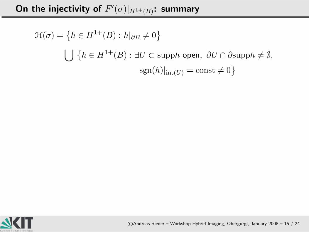
H(σ) =h ∈ H1+(B) : h|∂B 6= 0
⋃ h ∈ H1+(B) : ∃U ⊂ supph open, ∂U ∩ ∂supph 6= ∅,
sgn(h)|int(U) = const 6= 0

On the injectivity of F′(σ)|H1+(B): summary
c©Andreas Rieder – Workshop Hybrid Imaging, Obergurgl, January 2008 – 15 / 24
H(σ) =h ∈ H1+(B) : h|∂B 6= 0
⋃ h ∈ H1+(B) : ∃U ⊂ supph open, ∂U ∩ ∂supph 6= ∅,
sgn(h)|int(U) = const 6= 0
Theorem H(σ) ∩ N(F ′(σ)
)= ∅
On the injectivity of F′(σ)|H1+(B): conductivities not in H(σ)
c©Andreas Rieder – Workshop Hybrid Imaging, Obergurgl, January 2008 – 16 / 24
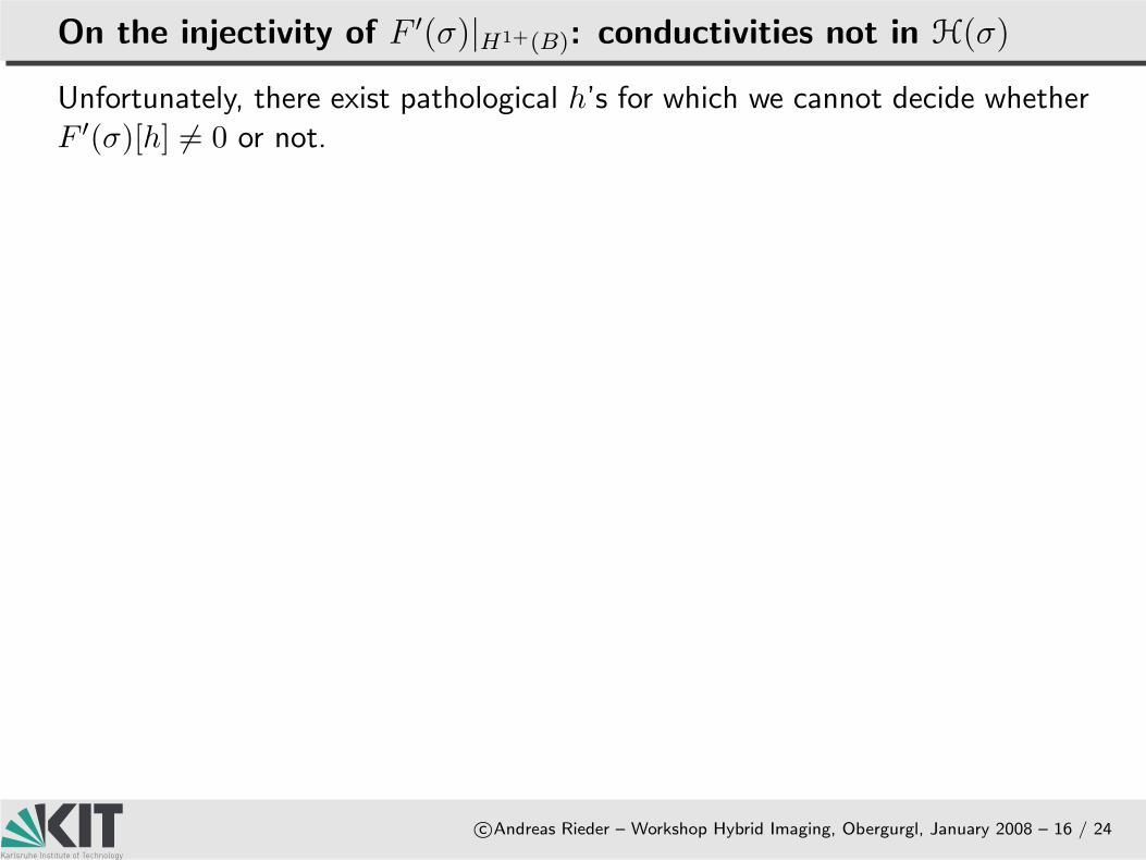
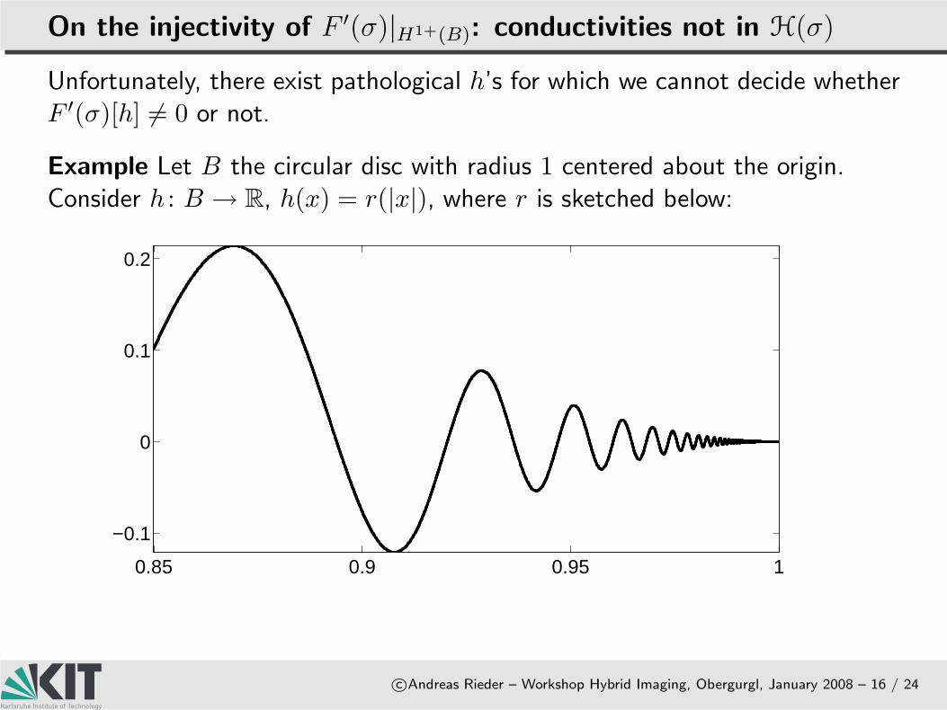
Unfortunately, there exist pathological h’s for which we cannot decide whetherF ′(σ)[h] 6= 0 or not.
On the injectivity of F′(σ)|H1+(B): conductivities not in H(σ)
c©Andreas Rieder – Workshop Hybrid Imaging, Obergurgl, January 2008 – 16 / 24
Unfortunately, there exist pathological h’s for which we cannot decide whetherF ′(σ)[h] 6= 0 or not.
Example Let B the circular disc with radius 1 centered about the origin.Consider h : B → R, h(x) = r(|x|), where r is sketched below:
0.85 0.9 0.95 1
−0.1
0
0.1
0.2
TCC for finite dimensional spaces
c©Andreas Rieder – Workshop Hybrid Imaging, Obergurgl, January 2008 – 17 / 24
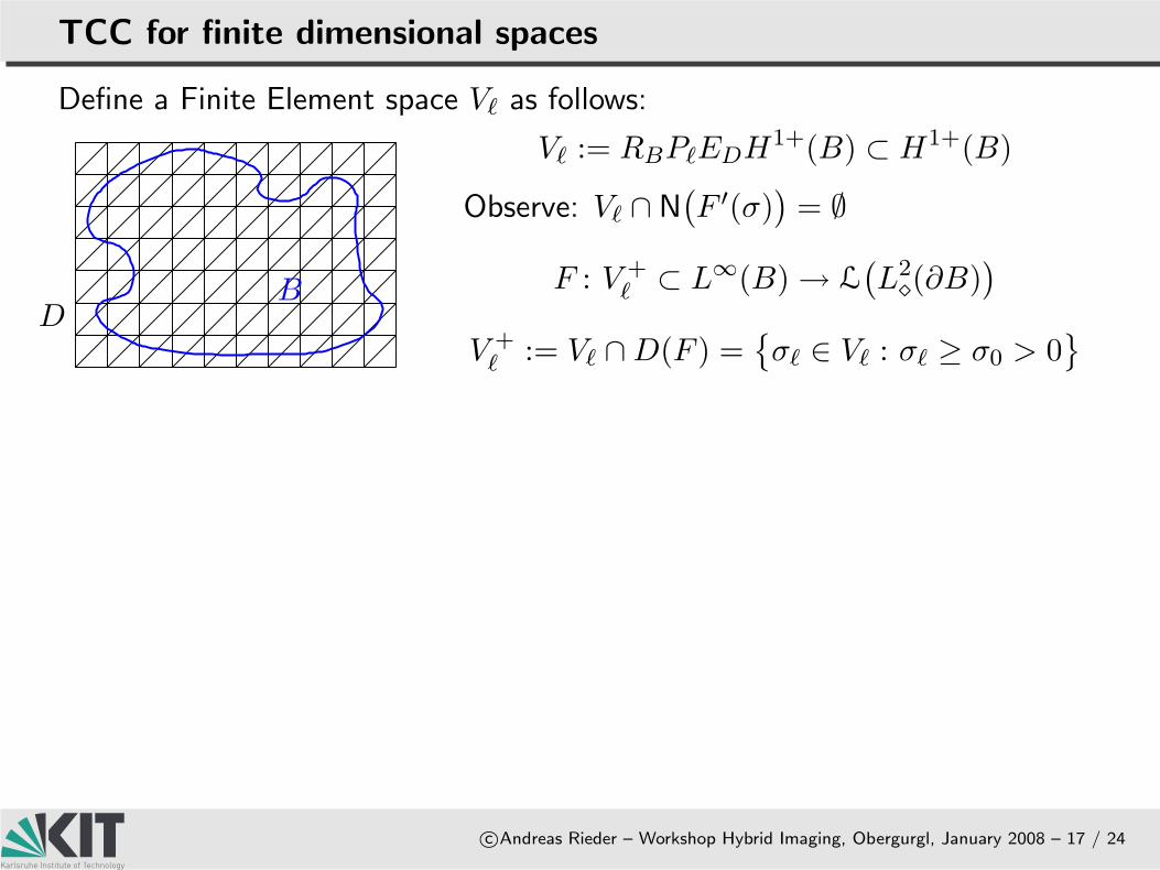
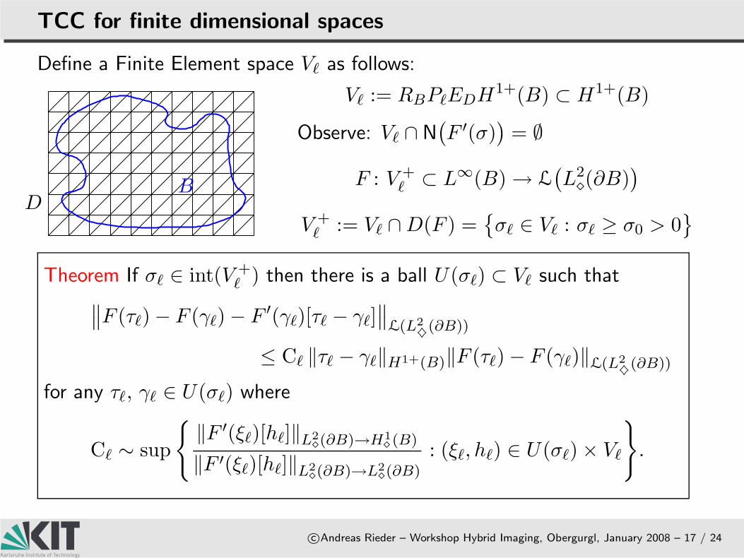
Define a Finite Element space V` as follows:
V` := RBP`EDH1+(B) ⊂ H1+(B)
Observe: V` ∩ N(F ′(σ)
)= ∅
F : V +` ⊂ L∞(B) → L
(L2(∂B)
)
V +` := V` ∩ D(F ) =
σ` ∈ V` : σ` ≥ σ0 > 0
DB
TCC for finite dimensional spaces
c©Andreas Rieder – Workshop Hybrid Imaging, Obergurgl, January 2008 – 17 / 24
Define a Finite Element space V` as follows:
V` := RBP`EDH1+(B) ⊂ H1+(B)
Observe: V` ∩ N(F ′(σ)
)= ∅
F : V +` ⊂ L∞(B) → L
(L2(∂B)
)
V +` := V` ∩ D(F ) =
σ` ∈ V` : σ` ≥ σ0 > 0
DB
Theorem If σ` ∈ int(V +` ) then there is a ball U(σ`) ⊂ V` such that
∥∥F (τ`) − F (γ`) − F ′(γ`)[τ` − γ`]
∥∥
L(L2♦
(∂B))
≤ C` ‖τ` − γ`‖H1+(B)‖F (τ`) − F (γ`)‖L(L2♦
(∂B))
for any τ`, γ` ∈ U(σ`) where
C` ∼ sup
‖F ′(ξ`)[h`]‖L2(∂B)→H1
(B)
‖F ′(ξ`)[h`]‖L2(∂B)→L2
(∂B)
: (ξ`, h`) ∈ U(σ`) × V`
.
EIT: Complete Electrode Model
The Tangential ConeCondition (TCC)
EIT: ContinuousModel
.EIT: CompleteElectrode Model
Conclusion
c©Andreas Rieder – Workshop Hybrid Imaging, Obergurgl, January 2008 – 18 / 24
Governing equation
c©Andreas Rieder – Workshop Hybrid Imaging, Obergurgl, January 2008 – 19 / 24
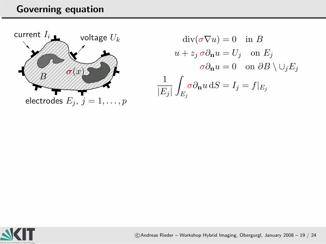
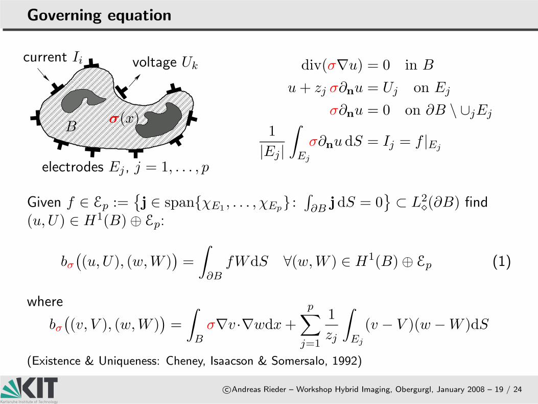
σ(x)
current Ii voltage Uk
electrodes Ej , j = 1, . . . , p
B
div(σ∇u) = 0 in B
u + zj σ∂nu = Uj on Ej
σ∂nu = 0 on ∂B \ ∪jEj
1
|Ej |
∫
Ej
σ∂nudS = Ij = f |Ej
Governing equation
c©Andreas Rieder – Workshop Hybrid Imaging, Obergurgl, January 2008 – 19 / 24
σ(x)
current Ii voltage Uk
electrodes Ej , j = 1, . . . , p
B
div(σ∇u) = 0 in B
u + zj σ∂nu = Uj on Ej
σ∂nu = 0 on ∂B \ ∪jEj
1
|Ej |
∫
Ej
σ∂nudS = Ij = f |Ej
Given f ∈ Ep :=j ∈ spanχE1
, . . . , χEp :∫
∂B jdS = 0⊂ L2
(∂B) find
(u, U) ∈ H1(B) ⊕ Ep:
bσ
((u, U), (w, W )
)=
∫
∂BfWdS ∀(w, W ) ∈ H1(B) ⊕ Ep (1)
where
bσ
((v, V ), (w, W )
)=
∫
Bσ∇v ·∇wdx +
p∑
j=1
1
zj
∫
Ej
(v − V )(w − W )dS
(Existence & Uniqueness: Cheney, Isaacson & Somersalo, 1992)
The forward operator
c©Andreas Rieder – Workshop Hybrid Imaging, Obergurgl, January 2008 – 20 / 24
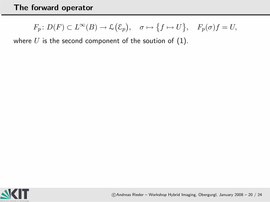
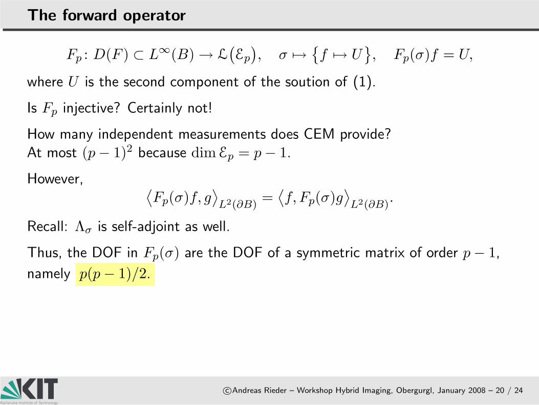
Fp : D(F ) ⊂ L∞(B) → L(Ep
), σ 7→
f 7→ U
, Fp(σ)f = U,
where U is the second component of the soution of (1).
The forward operator
c©Andreas Rieder – Workshop Hybrid Imaging, Obergurgl, January 2008 – 20 / 24
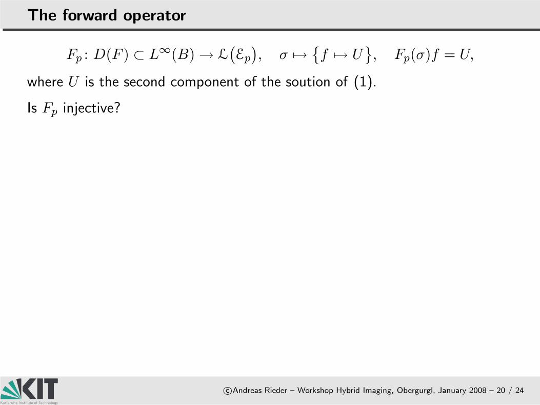
Fp : D(F ) ⊂ L∞(B) → L(Ep
), σ 7→
f 7→ U
, Fp(σ)f = U,
where U is the second component of the soution of (1).
Is Fp injective?
The forward operator
c©Andreas Rieder – Workshop Hybrid Imaging, Obergurgl, January 2008 – 20 / 24
Fp : D(F ) ⊂ L∞(B) → L(Ep
), σ 7→
f 7→ U
, Fp(σ)f = U,
where U is the second component of the soution of (1).
Is Fp injective? Certainly not!
The forward operator
c©Andreas Rieder – Workshop Hybrid Imaging, Obergurgl, January 2008 – 20 / 24
Fp : D(F ) ⊂ L∞(B) → L(Ep
), σ 7→
f 7→ U
, Fp(σ)f = U,
where U is the second component of the soution of (1).
Is Fp injective? Certainly not!
How many independent measurements does CEM provide?
The forward operator
c©Andreas Rieder – Workshop Hybrid Imaging, Obergurgl, January 2008 – 20 / 24
Fp : D(F ) ⊂ L∞(B) → L(Ep
), σ 7→
f 7→ U
, Fp(σ)f = U,
where U is the second component of the soution of (1).
Is Fp injective? Certainly not!
How many independent measurements does CEM provide?At most (p − 1)2 because dim Ep = p − 1.
However,⟨Fp(σ)f, g
⟩
L2(∂B)=
⟨f, Fp(σ)g
⟩
L2(∂B).
Recall: Λσ is self-adjoint as well.
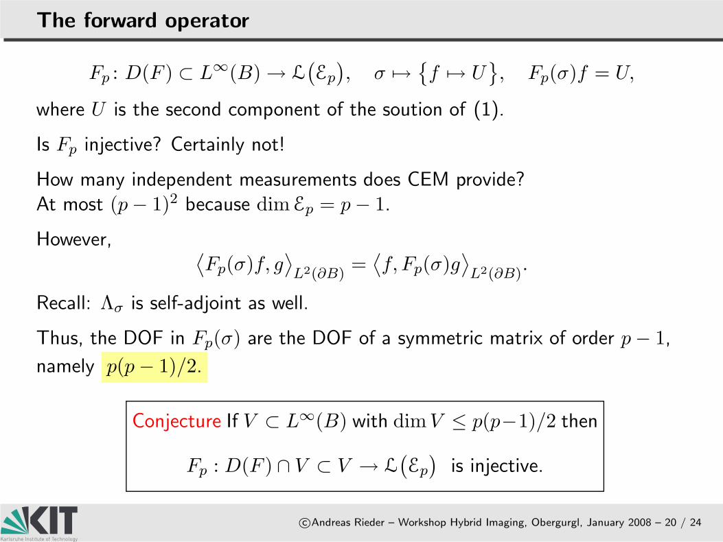
Thus, the DOF in Fp(σ) are the DOF of a symmetric matrix of order p − 1,
namely p(p − 1)/2.
The forward operator
c©Andreas Rieder – Workshop Hybrid Imaging, Obergurgl, January 2008 – 20 / 24
Fp : D(F ) ⊂ L∞(B) → L(Ep
), σ 7→
f 7→ U
, Fp(σ)f = U,
where U is the second component of the soution of (1).
Is Fp injective? Certainly not!
How many independent measurements does CEM provide?At most (p − 1)2 because dim Ep = p − 1.
However,⟨Fp(σ)f, g
⟩
L2(∂B)=
⟨f, Fp(σ)g
⟩
L2(∂B).
Recall: Λσ is self-adjoint as well.
Thus, the DOF in Fp(σ) are the DOF of a symmetric matrix of order p − 1,
namely p(p − 1)/2.
Conjecture If V ⊂ L∞(B) with dimV ≤ p(p−1)/2 then
Fp : D(F ) ∩ V ⊂ V → L(Ep
)is injective.
TCC for CEM
c©Andreas Rieder – Workshop Hybrid Imaging, Obergurgl, January 2008 – 21 / 24
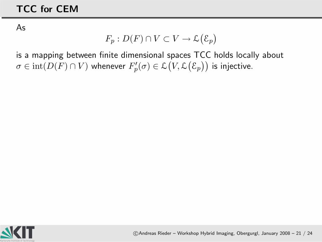
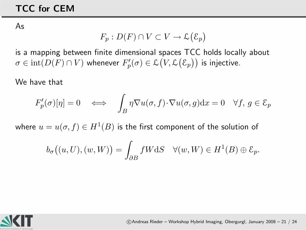
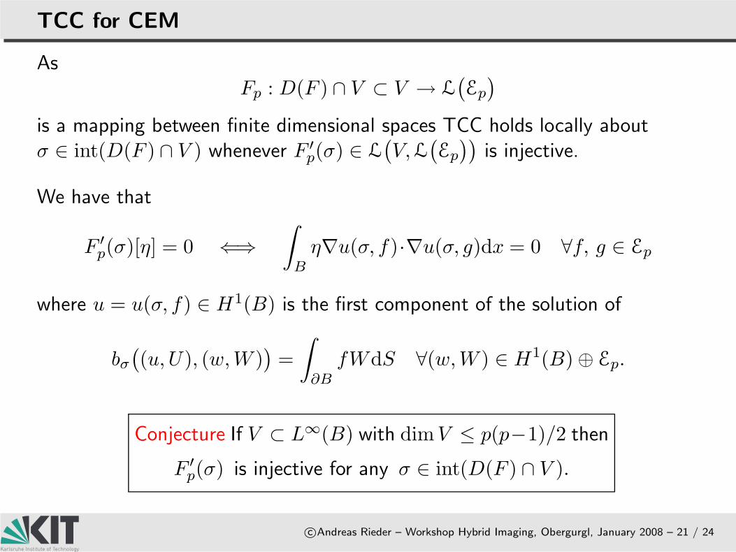
AsFp : D(F ) ∩ V ⊂ V → L
(Ep
)
is a mapping between finite dimensional spaces TCC holds locally aboutσ ∈ int(D(F ) ∩ V ) whenever F ′
p(σ) ∈ L(V, L
(Ep
))is injective.
TCC for CEM
c©Andreas Rieder – Workshop Hybrid Imaging, Obergurgl, January 2008 – 21 / 24
AsFp : D(F ) ∩ V ⊂ V → L
(Ep
)
is a mapping between finite dimensional spaces TCC holds locally aboutσ ∈ int(D(F ) ∩ V ) whenever F ′
p(σ) ∈ L(V, L
(Ep
))is injective.
We have that
F ′
p(σ)[η] = 0 ⇐⇒
∫
Bη∇u(σ, f)·∇u(σ, g)dx = 0 ∀f, g ∈ Ep
where u = u(σ, f) ∈ H1(B) is the first component of the solution of
bσ
((u, U), (w, W )
)=
∫
∂BfWdS ∀(w, W ) ∈ H1(B) ⊕ Ep.
Conjecture If V ⊂ L∞(B) with dimV ≤ p(p−1)/2 then
F ′
p(σ) is injective for any σ ∈ int(D(F ) ∩ V ).
Conclusion
The Tangential ConeCondition (TCC)
EIT: ContinuousModel
EIT: CompleteElectrode Model
. Conclusion
c©Andreas Rieder – Workshop Hybrid Imaging, Obergurgl, January 2008 – 22 / 24
What to remember from this talk
c©Andreas Rieder – Workshop Hybrid Imaging, Obergurgl, January 2008 – 23 / 24
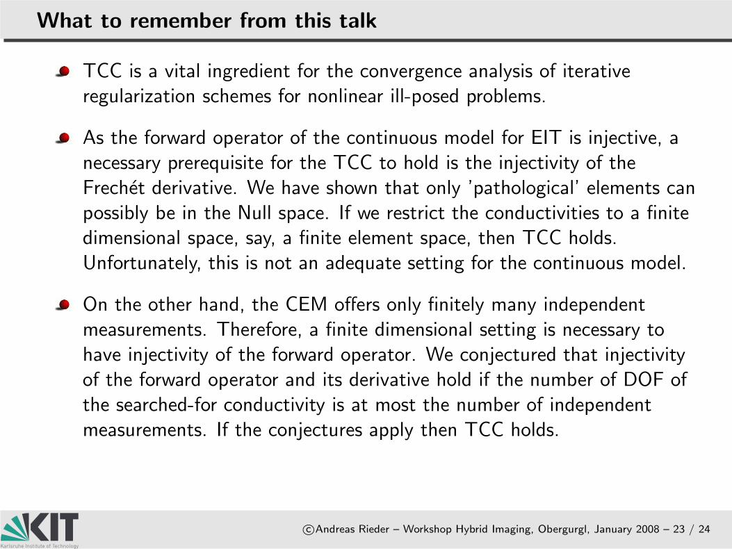
TCC is a vital ingredient for the convergence analysis of iterativeregularization schemes for nonlinear ill-posed problems.
As the forward operator of the continuous model for EIT is injective, anecessary prerequisite for the TCC to hold is the injectivity of theFrechet derivative. We have shown that only ’pathological’ elements canpossibly be in the Null space. If we restrict the conductivities to a finitedimensional space, say, a finite element space, then TCC holds.Unfortunately, this is not an adequate setting for the continuous model.
On the other hand, the CEM offers only finitely many independentmeasurements. Therefore, a finite dimensional setting is necessary tohave injectivity of the forward operator. We conjectured that injectivityof the forward operator and its derivative hold if the number of DOF ofthe searched-for conductivity is at most the number of independentmeasurements. If the conjectures apply then TCC holds.
What to remember from this talk
c©Andreas Rieder – Workshop Hybrid Imaging, Obergurgl, January 2008 – 23 / 24
TCC is a vital ingredient for the convergence analysis of iterativeregularization schemes for nonlinear ill-posed problems.
As the forward operator of the continuous model for EIT is injective, anecessary prerequisite for the TCC to hold is the injectivity of theFrechet derivative. We have shown that only ’pathological’ elements canpossibly be in the Null space. If we restrict the conductivities to a finitedimensional space, say, a finite element space, then TCC holds.Unfortunately, this is not an adequate setting for the continuous model.
On the other hand, the CEM offers only finitely many independentmeasurements. Therefore, a finite dimensional setting is necessary tohave injectivity of the forward operator. We conjectured that injectivityof the forward operator and its derivative hold if the number of DOF ofthe searched-for conductivity is at most the number of independentmeasurements. If the conjectures apply then TCC holds.
The Tangential ConeCondition (TCC)
EIT: ContinuousModel
EIT: CompleteElectrode Model
Conclusion
c©Andreas Rieder – Workshop Hybrid Imaging, Obergurgl, January 2008 – 24 / 24
Thank you for your attention!