gms tutorials modflow v. 10gmstutorials-10.4.aquaveo.com/modflow-modelcalibration.pdf · gms 10.4...

GMS Tutorials MODFLOW – Model Calibration

of 17 © Aquaveo 2018

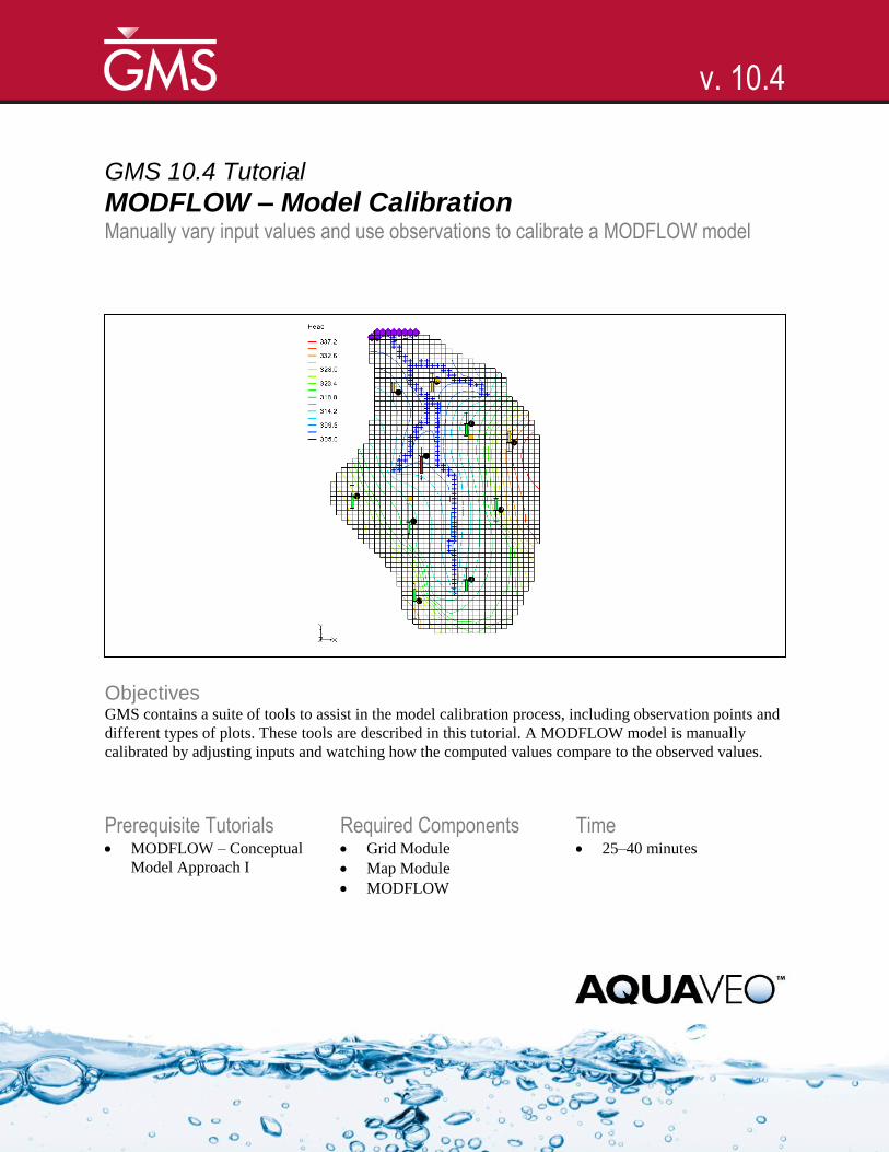
GMS 10.4 Tutorial

MODFLOW – Model Calibration Manually vary input values and use observations to calibrate a MODFLOW model

Objectives GMS contains a suite of tools to assist in the model calibration process, including observation points and

different types of plots. These tools are described in this tutorial. A MODFLOW model is manually

calibrated by adjusting inputs and watching how the computed values compare to the observed values.

Prerequisite Tutorials MODFLOW – Conceptual

Model Approach I

Required Components Grid Module

Map Module

MODFLOW

Time 25–40 minutes

v. 10.4



1 Introduction ......................................................................................................................... 2 1.1 Description of Problem ................................................................................................ 2 1.2 Getting Started ............................................................................................................. 4

2 Importing the Model ........................................................................................................... 4 3 Observation Data ................................................................................................................ 5 4 Entering Observation Points .............................................................................................. 5

4.1 Creating a Coverage with Observation Properties ........................................................ 5 4.2 Creating an Observation Point...................................................................................... 6 4.3 Calibration Target ........................................................................................................ 7 4.4 Point Statistics .............................................................................................................. 8

5 Reading in a Set of Observation Points ............................................................................. 8 5.1 Deleting the Observation Point .................................................................................... 8 5.2 Importing the Points ..................................................................................................... 8 5.3 Text Import Wizard ...................................................................................................... 9

6 Entering the Observed Stream Flow ............................................................................... 10 7 Viewing the Solution ......................................................................................................... 11

7.1 Error Summary ........................................................................................................... 11 7.2 Computed vs. Observed Data Plot.............................................................................. 12

8 Editing the Hydraulic Conductivity ................................................................................ 12 9 Converting the Model ....................................................................................................... 14 10 Computing a Solution ....................................................................................................... 14

10.1 Saving the Simulation ................................................................................................. 14 10.2 Running MODFLOW ................................................................................................. 14

11 Error vs. Simulation Plot .................................................................................................. 15 12 Continuing the Trial and Error Calibration................................................................... 16

12.1 Changing Values vs. Changing Zones ........................................................................ 16 12.2 Viewing the Answer ................................................................................................... 17

13 Conclusion.......................................................................................................................... 17

1 Introduction

An important part of any groundwater modeling exercise is the model calibration

process. In order for a groundwater model to be used in any type of predictive role, it

must be demonstrated that the model can successfully simulate observed aquifer

behavior. Calibration is a process wherein certain parameters of the model, such as

recharge and hydraulic conductivity, are altered in a systematic fashion and the model is

repeatedly run until the computed solution matches field-observed values within an

acceptable level of accuracy.

The model calibration exercise in this tutorial is based on the MODFLOW model. Thus,

it is recommended to complete the “MODFLOW – Conceptual Model Approach I”

tutorial prior to beginning this tutorial. Although this particular exercise is based on

MODFLOW, the calibration tools in GMS are designed in a general purpose fashion and

can be used with any model.

1.1 Description of Problem

A groundwater model for a medium-sized basin is shown in Figure 1. The basin

encompasses 72.5 square kilometers. It is in a semi-arid climate, with average annual

precipitation of 0.381 m/yr. Most of this precipitation is lost through evapotranspiration.



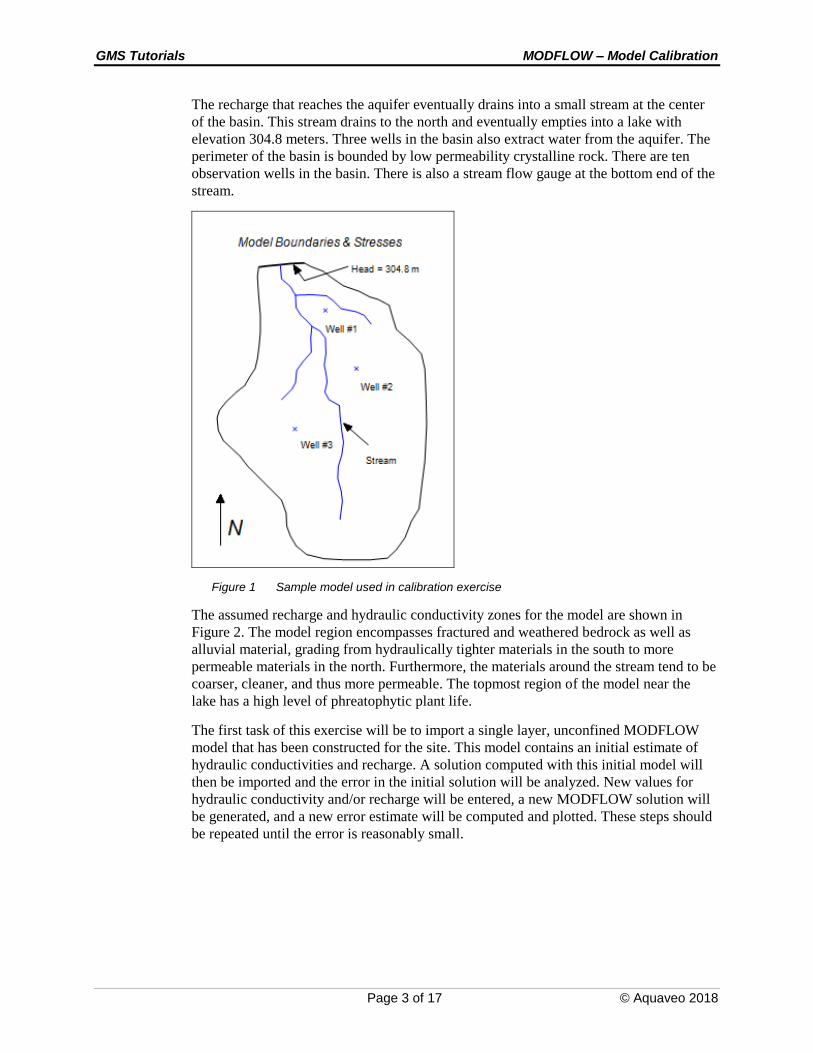
The recharge that reaches the aquifer eventually drains into a small stream at the center

of the basin. This stream drains to the north and eventually empties into a lake with

elevation 304.8 meters. Three wells in the basin also extract water from the aquifer. The

perimeter of the basin is bounded by low permeability crystalline rock. There are ten

observation wells in the basin. There is also a stream flow gauge at the bottom end of the

stream.

Figure 1 Sample model used in calibration exercise

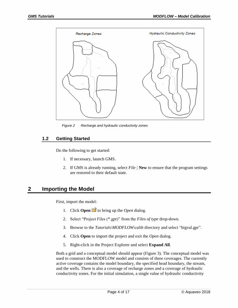
The assumed recharge and hydraulic conductivity zones for the model are shown in

Figure 2. The model region encompasses fractured and weathered bedrock as well as

alluvial material, grading from hydraulically tighter materials in the south to more

permeable materials in the north. Furthermore, the materials around the stream tend to be

coarser, cleaner, and thus more permeable. The topmost region of the model near the

lake has a high level of phreatophytic plant life.

The first task of this exercise will be to import a single layer, unconfined MODFLOW

model that has been constructed for the site. This model contains an initial estimate of

hydraulic conductivities and recharge. A solution computed with this initial model will

then be imported and the error in the initial solution will be analyzed. New values for

hydraulic conductivity and/or recharge will be entered, a new MODFLOW solution will

be generated, and a new error estimate will be computed and plotted. These steps should

be repeated until the error is reasonably small.



Figure 2 Recharge and hydraulic conductivity zones

1.2 Getting Started

Do the following to get started:

1. If necessary, launch GMS.

2. If GMS is already running, select File | New to ensure that the program settings

are restored to their default state.

2 Importing the Model

First, import the model:

1. Click Open to bring up the Open dialog.

2. Select “Project Files (*.gpr)” from the Files of type drop-down.

3. Browse to the Tutorials\MODFLOW\calib directory and select “bigval.gpr”.

4. Click Open to import the project and exit the Open dialog.

5. Right-click in the Project Explorer and select Expand All.

Both a grid and a conceptual model should appear (Figure 3). The conceptual model was

used to construct the MODFLOW model and consists of three coverages. The currently

active coverage contains the model boundary, the specified head boundary, the stream,

and the wells. There is also a coverage of recharge zones and a coverage of hydraulic

conductivity zones. For the initial simulation, a single value of hydraulic conductivity



(2.4 m/day) and a single value of recharge (7.62e-5 m/day) have been assigned. The

polygonal zones of hydraulic conductivity and recharge will be edited as the tutorial

progresses to reduce the model error.

Figure 3 Initial screen showing the model and three coverages

3 Observation Data

The tutorial will be using two types of observation data in the calibration process: water

table elevations from observation wells and observed flow rates in the stream. Since the

model is in a fairly arid region, assume that most of the flow to the stream is from

groundwater flow.

4 Entering Observation Points

First, it is necessary to enter a set of observation points representing the observed head in

the ten observation wells in the region. Observation points are created in the Map

module.

4.1 Creating a Coverage with Observation Properties

Before entering observation points, first create a coverage with observation properties.



1. Right-click on “ BigVal” in the Project Explorer and select New Coverage…

to bring up the Coverage Setup dialog.

2. Enter “Observation Wells” as the Coverage name.

3. In the Observation Points column, turn on Head.

4. Select “By layer number” from the 3D grid layer option for obs. pts drop-down.

5. Click OK to exit the Coverage Setup dialog.

4.2 Creating an Observation Point

It is now possible to create an observation point. To create the point, do the following:

1. Select the “ Observation wells” coverage to make it active.

2. Using the Create Point tool, click once anywhere on the model to create a

new point.

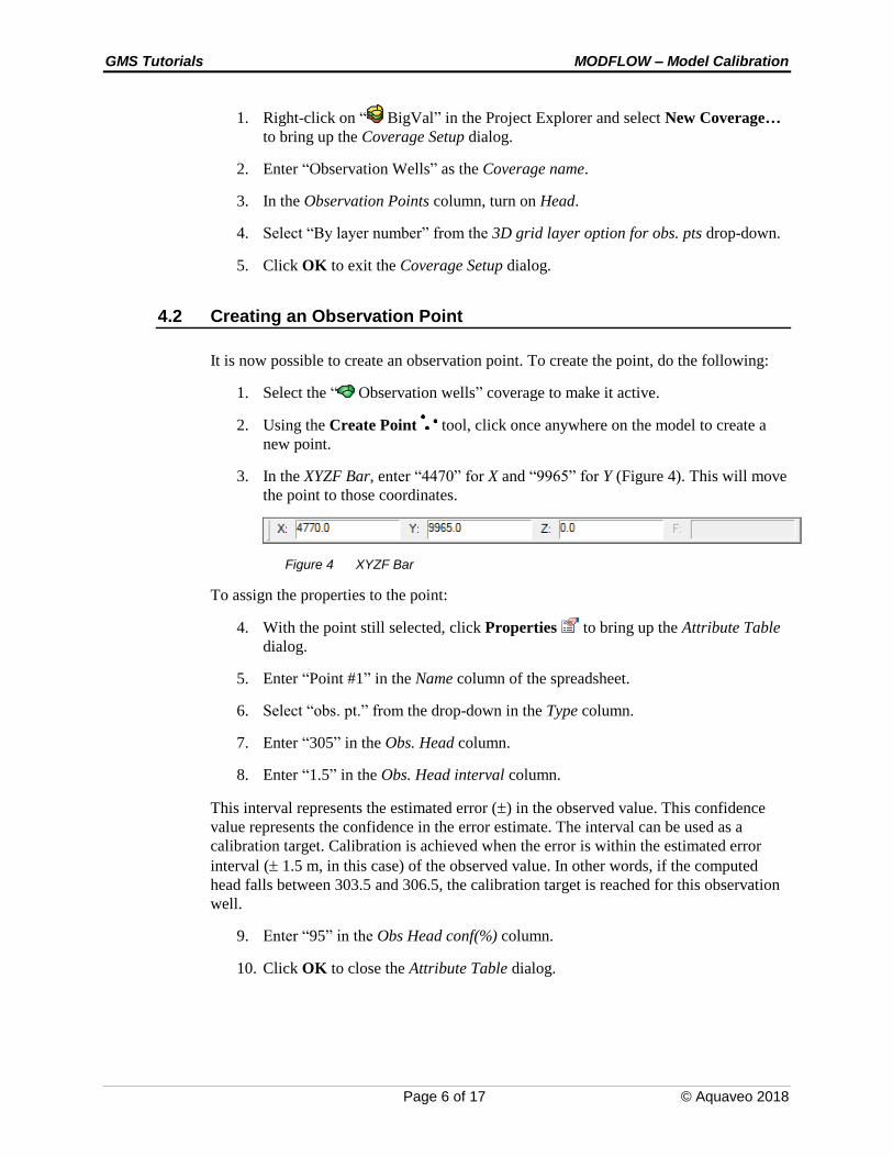
3. In the XYZF Bar, enter “4470” for X and “9965” for Y (Figure 4). This will move

the point to those coordinates.

Figure 4 XYZF Bar

To assign the properties to the point:

4. With the point still selected, click Properties to bring up the Attribute Table

dialog.

5. Enter “Point #1” in the Name column of the spreadsheet.

6. Select “obs. pt.” from the drop-down in the Type column.

7. Enter “305” in the Obs. Head column.

8. Enter “1.5” in the Obs. Head interval column.

This interval represents the estimated error () in the observed value. This confidence

value represents the confidence in the error estimate. The interval can be used as a

calibration target. Calibration is achieved when the error is within the estimated error

interval ( 1.5 m, in this case) of the observed value. In other words, if the computed

head falls between 303.5 and 306.5, the calibration target is reached for this observation

well.

9. Enter “95” in the Obs Head conf(%) column.

10. Click OK to close the Attribute Table dialog.



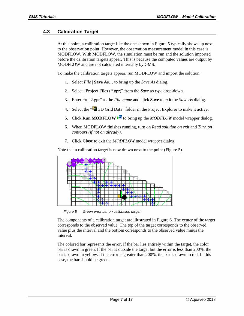
4.3 Calibration Target

At this point, a calibration target like the one shown in Figure 5 typically shows up next

to the observation point. However, the observation measurement model in this case is

MODFLOW. With MODFLOW, the simulation must be run and the solution imported

before the calibration targets appear. This is because the computed values are output by

MODFLOW and are not calculated internally by GMS.

To make the calibration targets appear, run MODFLOW and import the solution.

1. Select File | Save As… to bring up the Save As dialog.

2. Select “Project Files (*.gpr)” from the Save as type drop-down.

3. Enter “run2.gpr” as the File name and click Save to exit the Save As dialog.

4. Select the “ 3D Grid Data” folder in the Project Explorer to make it active.

5. Click Run MODFLOW to bring up the MODFLOW model wrapper dialog.

6. When MODFLOW finishes running, turn on Read solution on exit and Turn on

contours (if not on already).

7. Click Close to exit the MODFLOW model wrapper dialog.

Note that a calibration target is now drawn next to the point (Figure 5).

Figure 5 Green error bar on calibration target

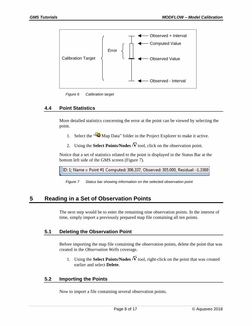
The components of a calibration target are illustrated in Figure 6. The center of the target

corresponds to the observed value. The top of the target corresponds to the observed

value plus the interval and the bottom corresponds to the observed value minus the

interval.

The colored bar represents the error. If the bar lies entirely within the target, the color

bar is drawn in green. If the bar is outside the target but the error is less than 200%, the

bar is drawn in yellow. If the error is greater than 200%, the bar is drawn in red. In this

case, the bar should be green.



Calibration Target

Error

Observed + Interval

Computed Value

Observed Value

Observed - Interval

Figure 6 Calibration target

4.4 Point Statistics

More detailed statistics concerning the error at the point can be viewed by selecting the

point.

1. Select the “ Map Data” folder in the Project Explorer to make it active.

2. Using the Select Points/Nodes tool, click on the observation point.

Notice that a set of statistics related to the point is displayed in the Status Bar at the

bottom left side of the GMS screen (Figure 7).

Figure 7 Status bar showing information on the selected observation point

5 Reading in a Set of Observation Points

The next step would be to enter the remaining nine observation points. In the interest of

time, simply import a previously prepared map file containing all ten points.

5.1 Deleting the Observation Point

Before importing the map file containing the observation points, delete the point that was

created in the Observation Wells coverage.

1. Using the Select Points/Nodes tool, right-click on the point that was created

earlier and select Delete.

5.2 Importing the Points

Now to import a file containing several observation points.




2. Select “Text Files (*.txt;*.csv)” from the Files of type drop-down.

3. Select “obswells.txt” and click Open to exit the Open dialog and bring up the

Step 1 of 2 page of the Text Import Wizard dialog.

5.3 Text Import Wizard

Opening a TXT file in GMS will bring up the Text Import Wizard. In the first step of the

wizard, it is necessary to identify the delimiters that separate the data into columns. In

the second step of the wizard, map the columns to fields that GMS recognizes.

1. In the section below the File import options section, turn on Heading row.

2. Click Next> to go to the Step 2 of 2 page of the Text Import Options dialog.

3. Select “Observation data” from the GMS data type drop-down.

Notice in the file preview section of the dialog that GMS has mapped the different

columns of data in the file into fields recognized by GMS. No changes need to be made

here.

4. Click Finish to import the observation data and close the Text Import Wizard

dialog.

Ten observation wells will appear (Figure 8).

Figure 8 The imported observation wells



6 Entering the Observed Stream Flow

Now that the observation points are defined, the observed flow in the stream can be

entered. Observed flows are assigned directly to arcs and polygons in the local

source/sink coverage of the conceptual model. MODFLOW determines the computed

flow from the aquifer to the stream. This flow value will be compared to the observed

flow.

GMS provides two methods for assigning observed flow: to individual arcs or to a group

of arcs. The stream flow that was measured at the site represents the total flow from the

aquifer to the stream at the stream outlet at the top of the model. This flow represents the

flow from the aquifer to the stream for the entire stream network. Thus, the observed

flow can be assigned to a group of arcs. When reading a solution, GMS will then

automatically sum the computed flow for all arcs in the group.

Before assigning the observed flow, first create an arc group:

1. Right-click on the “ Sources & Sinks” coverage and select Coverage Setup to

open the Coverage Setup dialog.

2. In the Sources/Sinks/BCs column, turn on Observed Flow.

3. Click OK to exit the Coverage Setup dialog.

4. Select “ Sources & Sinks” to make it active.

5. Using the Select Arcs tool while holding down the Shift key, click on each of

the river arcs. Be sure to select all six arcs.

6. Select Feature Object | Create Arc Group.

This creates a new object out of the selected objects. It is now possible to assign an

observed flow to the arc group.

7. Using the Select Arc Groups tool, double-click on any of the river arcs to

open the Attribute Table dialog.

8. Check the box in the Obs.flow column of the spreadsheet.

9. Enter “-4644” in the Obs. flow rate (m^3/d) column.

10. Enter “210” in the Obs. Flow interval column.

The entered values indicate that, to achieve calibration, the computed flow should be

between -4434 and -4854 m3/day (4644 +/- 210).

11. Click OK to exit the Attribute Table dialog.

12. Click outside the arc group to unselect it.

13. Save the project.

14. Select MODFLOW | Run MODFLOW to bring up the MODFLOW model

wrapper dialog.



15. When the model finishes running, turn on Read solution on exit and Turn on

contours (if not on already).

16. Click Close to exit the MODFLOW model wrapper dialog.

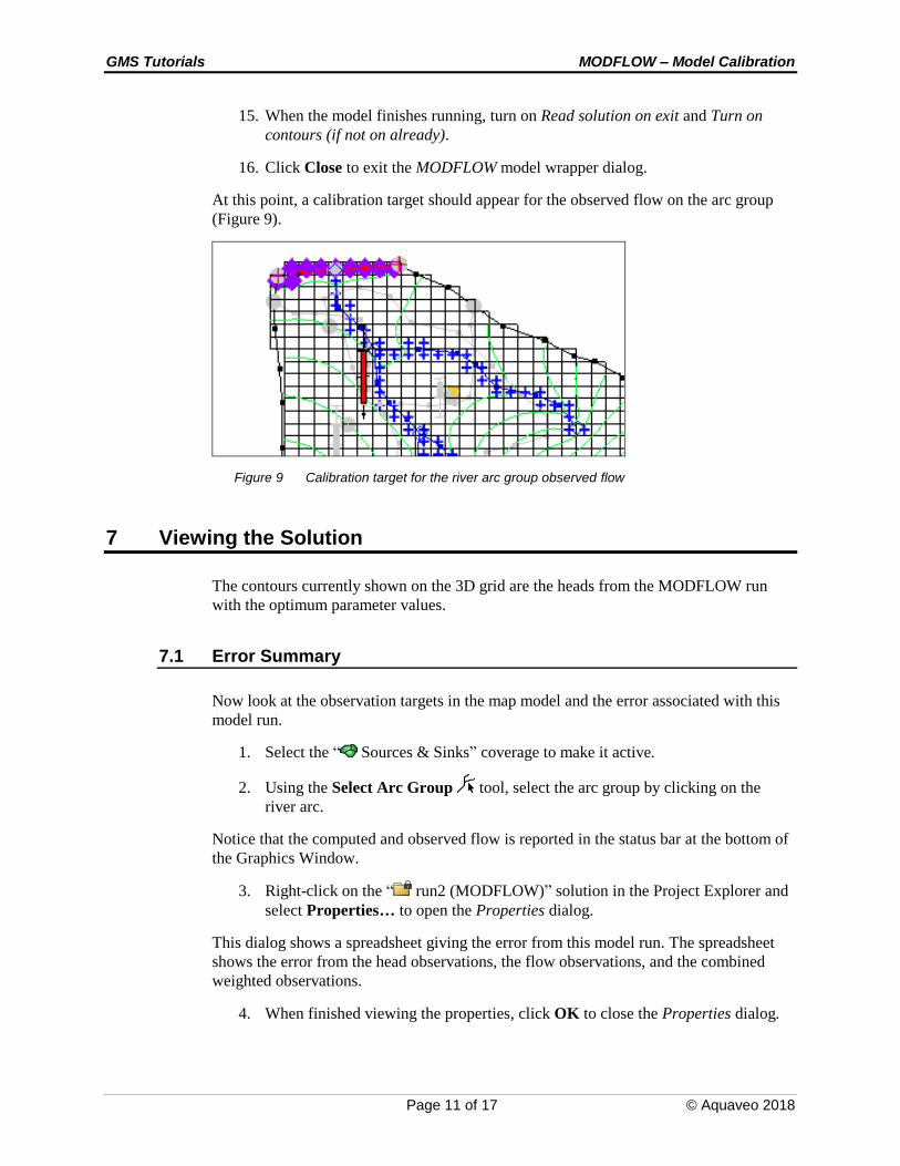
At this point, a calibration target should appear for the observed flow on the arc group

(Figure 9).

Figure 9 Calibration target for the river arc group observed flow

7 Viewing the Solution

The contours currently shown on the 3D grid are the heads from the MODFLOW run

with the optimum parameter values.

7.1 Error Summary

Now look at the observation targets in the map model and the error associated with this

model run.

1. Select the “ Sources & Sinks” coverage to make it active.

2. Using the Select Arc Group tool, select the arc group by clicking on the

river arc.

Notice that the computed and observed flow is reported in the status bar at the bottom of

the Graphics Window.

3. Right-click on the “ run2 (MODFLOW)” solution in the Project Explorer and

select Properties… to open the Properties dialog.

This dialog shows a spreadsheet giving the error from this model run. The spreadsheet

shows the error from the head observations, the flow observations, and the combined

weighted observations.

4. When finished viewing the properties, click OK to close the Properties dialog.



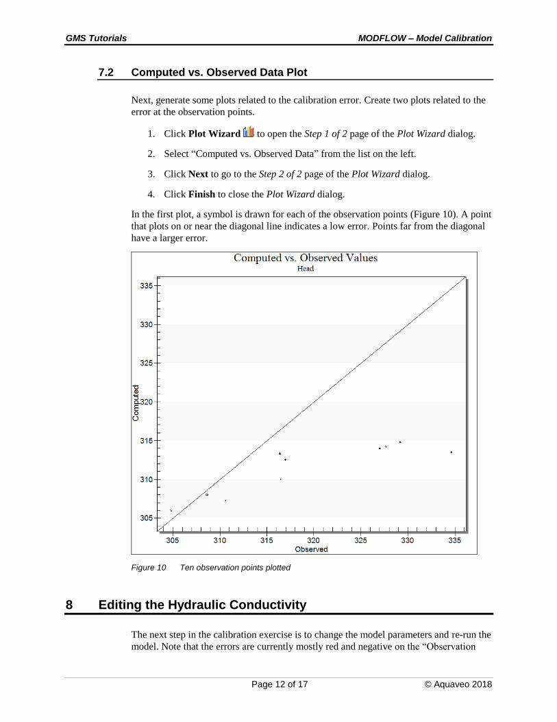
7.2 Computed vs. Observed Data Plot

Next, generate some plots related to the calibration error. Create two plots related to the

error at the observation points.

1. Click Plot Wizard to open the Step 1 of 2 page of the Plot Wizard dialog.

2. Select “Computed vs. Observed Data” from the list on the left.

3. Click Next to go to the Step 2 of 2 page of the Plot Wizard dialog.

4. Click Finish to close the Plot Wizard dialog.

In the first plot, a symbol is drawn for each of the observation points (Figure 10). A point

that plots on or near the diagonal line indicates a low error. Points far from the diagonal

have a larger error.

Figure 10 Ten observation points plotted

8 Editing the Hydraulic Conductivity

The next step in the calibration exercise is to change the model parameters and re-run the

model. Note that the errors are currently mostly red and negative on the “Observation



Wells” coverage. This indicates the observed value is much larger than the current

computed value. Begin with changing the hydraulic conductivity in these zones. Then

edit the hydraulic conductivity by changing the hydraulic conductivity assigned to the

polygonal zones in the conceptual model.

Before editing the hydraulic conductivity values, make the hydraulic conductivity zone

coverage the active coverage.

1. Select the “ Hydraulic Conductivity” coverage to make it active.

To edit the hydraulic conductivity values:

2. Using the Select Polygons tool while holding the Shift key, select polygons 1

and 2 as shown in Figure 11.

3. Click Properties to open the Attribute Table dialog.

4. On the All row, enter “0.6” in the Horizontal K (m/d) column. This changes the

value for both polygons at the same time.


6. Double-click on polygon 3 as shown in Figure 11 to open the Attribute Table

dialog.

7. Enter “0.15” in the Horizontal K column.


9. Click outside the model to unselect the polygon.

3

2

1

Figure 11 Polygons to be selected.



9 Converting the Model

Now that the values have been edited, the next step is to convert the conceptual model to

the grid-based numerical model:

1. Click Map → MODFLOW to bring up the Map → Model dialog.

2. Select All applicable coverages and click OK to close the Map → Model dialog.

10 Computing a Solution

The next step is to save the MODFLOW model with the new values and compute a new

solution.

10.1 Saving the Simulation

To save the simulation:

1. Select File | Save As… to bring up the Save As dialog.

2. Select “Project Files (*.gpr)” from the Save as type drop-down.

3. Enter “run3.gpr” as the File name.

4. Click Save to close the Save As dialog.

10.2 Running MODFLOW

Do the following to run MODFLOW:

1. Click Run MODFLOW to bring up the MODFLOW model wrapper dialog.

2. When the MODFLOW simulation is completed, turn on Read solution on exit

and Turn on contours (if not on already).

3. Click Close to import the solution and close the MODFLOW model wrapper

dialog.

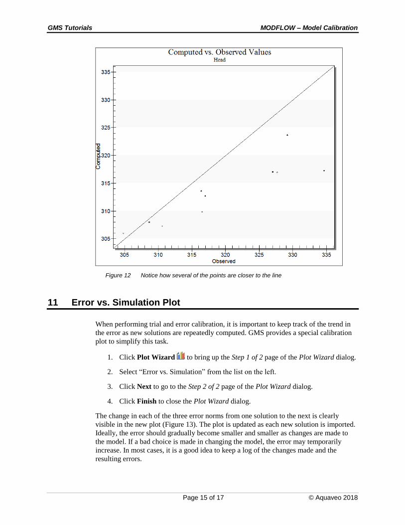
Note that the plot in the Plot Window has been updated (Figure 12). Although the error

improved for the observation wells, the head is still too low on the left and right sides of

the model. Up to this point, the tutorial has not paid much attention to the flow target on

the arc group. In the next section, create a plot that shows how well the flow target is

being met.



Figure 12 Notice how several of the points are closer to the line

11 Error vs. Simulation Plot

When performing trial and error calibration, it is important to keep track of the trend in

the error as new solutions are repeatedly computed. GMS provides a special calibration

plot to simplify this task.

1. Click Plot Wizard to bring up the Step 1 of 2 page of the Plot Wizard dialog.

2. Select “Error vs. Simulation” from the list on the left.

3. Click Next to go to the Step 2 of 2 page of the Plot Wizard dialog.

4. Click Finish to close the Plot Wizard dialog.

The change in each of the three error norms from one solution to the next is clearly

visible in the new plot (Figure 13). The plot is updated as each new solution is imported.

Ideally, the error should gradually become smaller and smaller as changes are made to

the model. If a bad choice is made in changing the model, the error may temporarily

increase. In most cases, it is a good idea to keep a log of the changes made and the

resulting errors.



5. When finished viewing the plot, close the plot window.

Figure 13 The change in error is more clearly visible

12 Continuing the Trial and Error Calibration

At this point, continue with the trial-and-error calibration process using the steps

outlined above. If changing the recharge and the hydraulic conductivity values, be sure to

make the coverage visible by selecting it in the Project Explorer.

12.1 Changing Values vs. Changing Zones

For this tutorial, a good match between the computed and observed values can be

obtained simply by changing the hydraulic conductivity and recharge values assigned to

the polygonal zones. In a real application, however, the size and distribution of the zones

may need to be changed in addition to the values assigned to the zones.



12.2 Viewing the Answer

To view the “answer,” a map file can be imported that contains a set of parameter values

that result in a solution that satisfies the calibration target for each of the ten observation

wells.

Before importing the new conceptual model, delete the “BigVal” conceptual model:

1. Right-click on the “ BigVal” conceptual model and select Delete.

To import the new conceptual model:


3. Select “Map Files (*.map)” from the Files of type drop-down.

4. Select “answer.map”.

5. Click Open to import the project and close the Open dialog.

This model can now be converted to the grid, and a new solution can be computed using

the steps described above.

13 Conclusion

This concludes the “MODFLOW – Model Calibration” tutorial. The following key

topics were discussed and demonstrated:

Observation points will display a target next to them that shows how well the

computed values match the observed values.

With MODFLOW, the computed values at the observation points come from

MODFLOW and not GMS. Thus, if creating an observation point, MODFLOW

will have to be run before seeing a target.

If wanting to specify a flow observation that applies to a network of streams,

create an arc group.

A number of different plots are available when doing model calibration.

It is possible to import data from another GMS project by turning on Import into

current project in the Open dialog after selecting the desired project.

Whenever changes are made to the conceptual model, the Feature Objects | Map

→ MODFLOW command must be used and the project must be saved before

running MODFLOW.

gms tutorials modflow v. 10gmstutorials-10.4.aquaveo.com/modflow-modelcalibration.pdf · gms 10.4...

Documents