gms tutorials modflow-usg v. 10.4...

$: GMS Tutorials MODFLOW-USG v. 10.4 Calibrationgmstutorials-10.4.aquaveo.com/MODFLOW-USG-Calibration.pdf · USG\Calibration\calib-usg_MODFLOW-ugrid directory in Windows Explorer. This$
GMS Tutorials MODFLOW-USG – Calibration

Page 1 of 15 © Aquaveo 2018

GMS 10.4 Tutorial

MODFLOW-USG – Calibration Generate observation data in a MODFLOW-USG model

Objectives Learn how to use the GMS tools to create observation data for MODFLOW-USG.

Prerequisite Tutorials MODFLOW – Model

Calibration

MODFLOW-USG –

Quadtree

Required Components Grid

Map

MODFLOW

Time 15–30 minutes

v. 10.4

GMS Tutorials MODFLOW-USG – Calibration


1 Introduction ......................................................................................................................... 2 2 Getting Started .................................................................................................................... 3

2.1 Importing the Starting Project ...................................................................................... 3 2.2 Saving with a Different Name ...................................................................................... 4

3 Converting to MODFLOW-USG ....................................................................................... 4 4 Generating Observation Data for MODFLOW-USG ...................................................... 5 5 Saving and Running MODFLOW ..................................................................................... 7

5.1 Viewing the Model Error ............................................................................................. 8 5.2 Changing the Observation Target Display Options ...................................................... 9

6 Creating a MODFLOW-USG Model on a Voronoi UGrid ........................................... 10 6.1 Creating the UGrid ..................................................................................................... 10 6.2 Creating the MODFLOW-USG Simulation ............................................................... 11 6.3 Saving and Running MODFLOW-USG ..................................................................... 12

7 Creating a MODFLOW-USG Model on a Quadtree UGrid ......................................... 12 7.1 Creating the UGrid ..................................................................................................... 12 7.2 Creating the MODFLOW-USG Simulation ............................................................... 13 7.3 Saving and Running MODFLOW-USG ..................................................................... 14

8 Conclusion.......................................................................................................................... 14 9 References .......................................................................................................................... 15

1 Introduction

An important part of any groundwater modeling exercise is the model calibration

process. In order for a groundwater model to be used in any type of predictive role, it

must be demonstrated that the model can successfully simulate observed aquifer

behavior. Calibration is a process wherein certain parameters of the model, such as

recharge and hydraulic conductivity, are altered in a systematic fashion. Then, the model

is repeatedly run until the computed solution matches field-observed values within an

acceptable level of accuracy.

Most versions of MODFLOW include an observation process within the model.

MODFLOW-USG does not, so the steps to set up observation data vary slightly from

other versions of MODFLOW. Various utility programs have been developed as part of

the PEST suite of tools. They are used to compute observation data with MODFLOW-

USG. After MODFLOW-USG successfully runs a model, these PEST utilities are used

to post-process the MODFLOW outputs in order to compare the model simulated values

with the field-observed values.

This tutorial starts with a MODFLOW 2000 model that includes observation data, and

converts that model to a MODFLOW-USG model. Different types of UGrids are

generated using the same conceptual model to show how observations work with

Quadtree and Voronoi grids.

Familiarity with conceptual modeling, model calibration, MODFLOW-USG, and

unstructured grid generation is assumed. The prerequisite tutorials should be completed

prior to starting this tutorial.

This tutorial discusses and demonstrates opening a MODFLOW 2000 model and

converting it to a MODFLOW-USG simulation. It then generates observation data for the

MODFLOW-USG model, runs MODFLOW-USG, and reviews the results. Creation of a

GMS Tutorials MODFLOW–USG – Calibration


Voronoi UGrid and MODFLOW-USG simulation, as well as quadtree UGrid and

MODFLOW-USG simulation, will be shown.

2 Getting Started

Do the following to get started.

1. If necessary, launch GMS.

2. If GMS is already running, select File | New to ensure that the program settings

are restored to their default state.

2.1 Importing the Starting Project

Begin by importing a previously constructed MODFLOW-2000 model.

1. Click Open to bring up the Open dialog.

2. Select “Project Files (*.gpr)” from the Files of type drop-down.

3. Browse to the Tutorials\MODFLOW-USG\Calibration\ directory and select

“bigval.gpr”.

4. Click Open to import the project and exit the Open dialog.

A model similar to Figure 1 should appear.

Figure 1 MODFLOW-2000 model



The model has observation wells with calibration targets displayed next to each point.

There is also a flow observation associated with the river boundary condition (blue

symbols).

2.2 Saving with a Different Name

Before making any changes, save the project under a new name.

1. Select File | Save As… to bring up the Save As dialog.

2. Select “Project Files (*.gpr)” from the Save as type drop-down.

3. Enter “calib-usg.gpr” as the File name.

4. Click Save to save the project under the new name and close the Save As dialog.

It is recommended to Save periodically while progressing through the model.

3 Converting to MODFLOW-USG

Now to create a MODFLOW-USG model from the MODFLOW 2000 model.

1. Right-click on the “ MODFLOW” in the Project Explorer and select Convert

to MODFLOW-USG Simulation.

2. Click No when prompted to include inactive cells in the new UGrid.

3. Click OK when prompted regarding the PCG package not being copied to the

MODFLOW-USG simulation.

The PCG package is a solver package that is not supported in USG. USG supports the

SMS solver package and this has been included in the new simulation.

4. Turn off the “ 3D Grid Data” folder in the Project Explorer to hide the 3D

Grid.

Notice that the UGrid looks identical to the 3D Grid but is not displaying any contours

(Figure 2). The calibration targets are still visible and are showing the computed values

from the MODFLOW-2000 model on the 3D Grid.



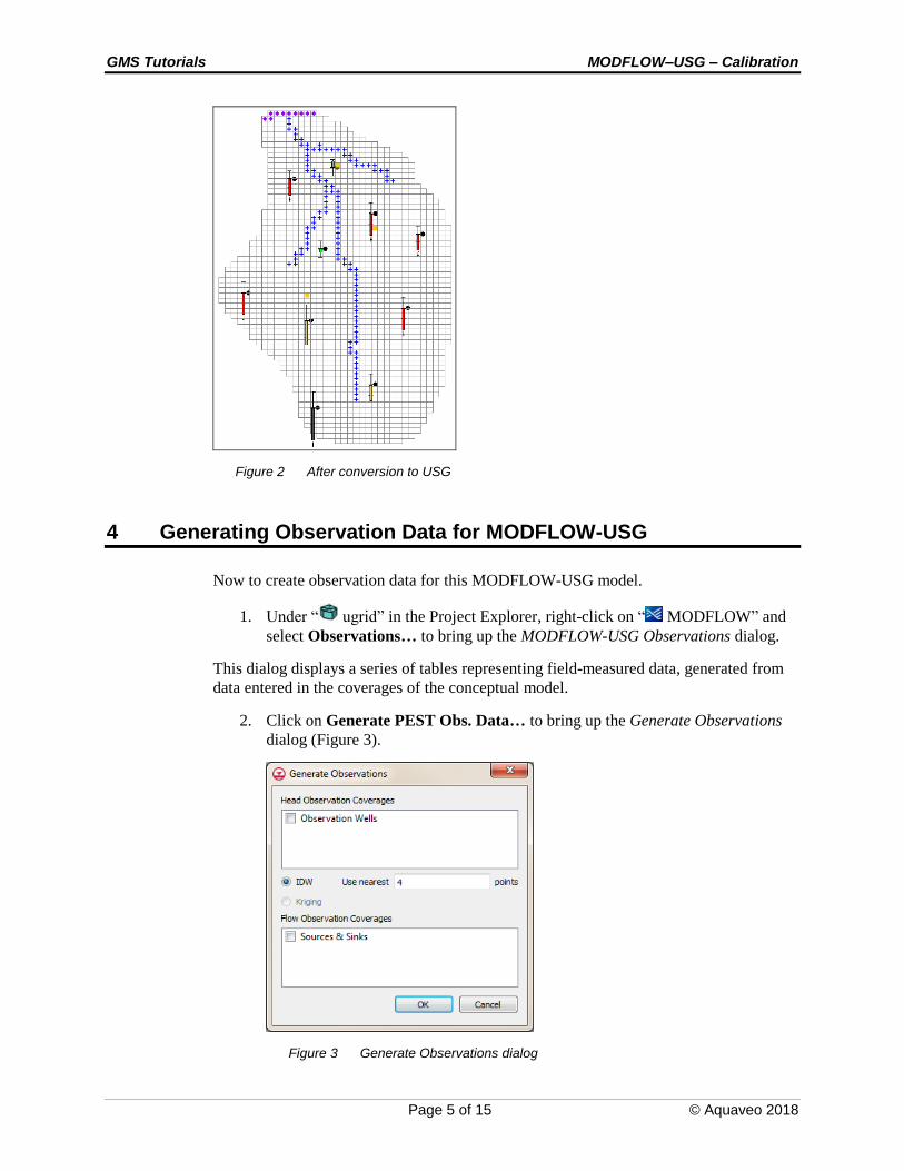
Figure 2 After conversion to USG

4 Generating Observation Data for MODFLOW-USG

Now to create observation data for this MODFLOW-USG model.

1. Under “ ugrid” in the Project Explorer, right-click on “ MODFLOW” and

select Observations… to bring up the MODFLOW-USG Observations dialog.

This dialog displays a series of tables representing field-measured data, generated from

data entered in the coverages of the conceptual model.

2. Click on Generate PEST Obs. Data… to bring up the Generate Observations

dialog (Figure 3).

Figure 3 Generate Observations dialog



The dialog allows choosing from the coverages in the current project that have

observation data. In this case, two coverages have observation data. Head measurements

are in the “Observation Wells” coverage and flow measurements are in the “Sources &

Sinks” coverage.

Notice that below the Head Observation Coverages section, there is an option to select

an interpolation scheme (IDW, Kriging). This is used to interpolate from the model grid

cells to the observation wells.

3. In the Head Observation Coverages section, turn on “Observation Wells”.

4. In the Flow Observation Coverages section, turn on “Sources & Sinks”.

5. Leave all other options at the defaults and click OK to generate the observation

data.

A new “Wells” table should be visible in the right side of the dialog (Figure 4).

Figure 4 MODFLOW-USG Observations dialog Wells table

The items in this table represent the observation well data found in the “Observation

Wells” coverage, showing the coverage name, point id, and point name. The last column

is an alias. The PEST utilities used to compute observation information have certain

rules for the names of observations. The alias column ensures that these rules are met

without any required interaction. If the user-defined name assigned to the point meets

these rules, then the user-defined name will be used as the alias.

6. Select “Well To Node” from the list on the left.



The entries in this table represent the interpolation from the UGrid cells to the

observation point. The table shows the alias of the well, the UGrid cell id (Node ID), and

an interpolation factor. The PEST utility uses the cell ids and factors to interpolate from

the MODFLOW head output file to each observation well.

7. Select “Well Sample” from the list on the left.

This table represents the measurements taken at the observation wells. The table lists a

well alias, a date/time, and a head value. If the model was transient, it would most likely

have multiple measurements at each well with a different date/time for each

measurement. Since this model is steady state, only one measurement for each well and

the date of 1950-01-01 00:00:00 has been assigned. The date is meaningless in this case,

but a date must be assigned for the PEST utility to function so GMS uses this date as the

default.

8. Select “Flow Observations” from the list on the left.

This table lists any flow observations that are included in the coverages of the conceptual

model and is similar to the “Wells” table. The table lists the coverage name, the type of

feature (i.e., POINT, ARC, ARCGROUP, POLYGON), the feature ID, the feature name,

and an alias. This alias is just like the alias for the observations wells. In this model,

notice that one flow observation is on an arcgroup. This arc group comprises several arcs

that are used to define the river in the middle of the model.

9. Select “Flow Sample” from the list on the left.

This table lists the flow measurements taken from field data. It is just like the “Well

Sample” table.

10. Click OK to exit the MODFLOW-USG Observations dialog.

5 Saving and Running MODFLOW

Now to run MODFLOW.

1. Save the project.

2. Right-click on the “ MODFLOW” item under “ ugrid” item and select

Open Containing Folder to bring up the \Tutorials\MODFLOW-

USG\Calibration\calib-usg_MODFLOW-ugrid directory in Windows Explorer.

This is the directory where the MODFLOW-USG input files are saved. Notice that there

are several files with “calib-usg.obsusg.” and “calib-usg.obsusgf.” as part of the file

name. These are not MODFLOW input files, but are used as inputs for the PEST

utilities.

There are also several batch files in the folder. These batch files are used to call the

PEST utilities after MODFLOW runs. The main batch file is named “usgobs.bat”. This is

the batch file that runs once MODFLOW has terminated successfully

3. Close Windows Explorer and return to GMS.



4. Click Run MODFLOW to bring up the MODFLOW model wrapper dialog.

5. When the model finishes, turn on Read solution on exit and Turn on contours (if

not on already).

6. Click Close to import the solution, close the MODFLOW model wrapper dialog,

and bring up a GMS prompt.

The prompt states that “The current project includes both a 3D Grid and a UGrid. The

observation targets will be drawn using data from the active dataset on the active 3D

Grid. This display option can be edited in the Map Data Display Options under the

section ‘Projects including 3D Grid & UGrid, MODFLOW targets use’.”

7. Click OK to close the prompt.

The model should update to appear similar to Figure 5.

Figure 5 Contours after the initial MODFLOW run

5.1 Viewing the Model Error

Now to compare the model error for the MODFLOW-USG model to the MODFLOW-

2000 model.

1. Right-click on the “ calib-usg (MODFLOW)” solution and select

Properties… to bring up the Properties dialog.



The values should match those shown in Figure 6.

Figure 6 Model error for MODFLOW-USG model

2. Select OK to exit the Properties dialog.

3. Right-click on the “ bigval (MODFLOW)” solution under “ grid” and

select Properties… to bring up the Properties dialog.

The values should match those shown in Figure 7. Note that the error is slightly different

for the two models. This is expected since this MODFLOW-USG model is a copy of the

3D grid model. The difference in the observations comes by using the PEST utilities to

calculate the computed values instead of using the MODFLOW OBS package.

Figure 7 Model error for MODFLOW-2000 model

4. Select OK to exit the Properties dialog.



5.2 Changing the Observation Target Display Options

Now to change the display options so that the targets will reflect the computed values

from the MODFLOW-USG simulation.

1. Click Display Options to bring up the Display Options dialog.

2. Select “ Map Data” from the list on the left.

3. On the Map tab at the bottom of the section on the right, select “UGrid” from the

Project including 3D Grid & UGrid, MODFLOW targets use drop-down.

4. Click OK to exit the Display Options dialog.

As expected, the targets look nearly the same as the targets did when using the data from

the 3D grid. If there is only a 3D Grid or only a UGrid, then this display option has no

effect on the observation points. However, when a project has both a 3D Grid

MODFLOW simulation and a UGrid MODFLOW simulation, this display option is used

to determine the source of the computed values for the observation points.

6 Creating a MODFLOW-USG Model on a Voronoi UGrid

Now to create a second UGrid using the Voronoi criteria.

6.1 Creating the UGrid

1. Right-click on “ 3D Grid Data” in the Project Explorer and select Delete.

Deleting the 3D Grid before creating Voronoi and quadtree UGrids with corresponding

MODFLOW-USG simulations avoids the message about having both a 3D Grid and a

UGrid associated with the observation data.

2. Select “ Sources & Sinks” in the Project Explorer to make it active.

3. Right-click on “ Sources & Sinks” and select Map To | UGrid to bring up the

Map → UGrid dialog.

4. Select “3D” from the Dimension drop-down.

5. Select “Voronoi” from the UGrid type drop-down.

6. Enter “1” in the Number of cells field in the Z-Dimension section.

7. Click OK to close the Map → UGrid dialog.

8. Uncheck the box next to “ ugrid” in the Project Explorer to better see the

newly created “ ugrid (2)”.

The new UGrid should be similar to Figure 8.



Figure 8 Voronoi UGrid

6.2 Creating the MODFLOW-USG Simulation

Now to create a MODFLOW-USG simulation on the UGrid. Start with creating a new

MODFLOW simulation. Then, use the layer interpolation tools to set the elevations of

the grid and convert the conceptual model by mapping it to MODFLOW.

1. Right-click on “ ugrid (2)” and select Rename.

2. Enter “voronoi” and press Enter to set the new name.

3. Right-click on “ voronoi” and select New MODFLOW… to bring up the

MODFLOW Global/Basic Package dialog.

4. Click OK to exit the MODFLOW Global/Basic Package dialog.

5. Right-click on “ Layers” and select Interpolate to | MODFLOW Layers to

bring up the Interpolate to MODFLOW Layers dialog.

6. Click OK to accept the defaults, close the Interpolate to MODFLOW Layers

dialog, and interpolate the layer elevations to “ voronoi”.

7. Right-click on “ BigVal” and select Map to | MODFLOW/MODPATH to

bring up the Map → Model dialog.

8. Click OK to accept the defaults, close the Map → Model dialog, and convert the

conceptual model to “ voronoi”. This process may take a few moments.



9. Right-click on “ MODFLOW” under “ voronoi” and select

Observations… to bring up the MODFLOW-USG Observations dialog.

Notice that the observation data has already been populated. This happens as part of

mapping the data to MODFLOW.

10. Click Generate PEST Obs. Data… to bring up the Generate Observations

dialog.

Notice that both coverages listed have a check next to them.

11. Click OK to exit the Generate Observations dialog.


6.3 Saving and Running MODFLOW-USG

Now to run MODFLOW using the Voronoi UGrid.




not on already).

4. Click Close to import the solution and exit the MODFLOW model wrapper

dialog.

5. Select the “ Observation Wells” coverage to make the observation targets

visible.

Notice that the observation targets are similar to those in the original model.

7 Creating a MODFLOW-USG Model on a Quadtree UGrid

Now to create the quadtree UGrid and its corresponding MODFLOW-USG simulation.

7.1 Creating the UGrid

1. Select “ Sources & Sinks” to make it active.

2. Right-click on “ Sources & Sinks” and select Map To | UGrid to bring up the

Map → UGrid dialog.

3. Select “3D” from the Dimension drop-down.

4. Select “Quadtree / Octree” from the UGrid type drop-down.



5. In both the X-Dimension and Y-Dimension sections, select the Cell size option

and enter “200.0” in the Cell size field.

6. Click OK to close the Map → UGrid dialog.

7. Turn off “ voronoi” to better view the new “ ugrid (2)”.

The new UGrid should appear similar to Figure 9.

Figure 9 Quadtree UGrid

7.2 Creating the MODFLOW-USG Simulation

Now to create a MODFLOW-USG simulation using the procedure show in section 6.2.

1. Right-click on “ ugrid (2)” and select Rename.

2. Enter “quadtree” and press Enter to set the new name.

3. Right-click on “ quadtree” and select New MODFLOW… to bring up the

MODFLOW Global/Basic Package dialog.

4. Click OK to exit the MODFLOW Global/Basic Package dialog.

5. Right-click on “ Layers” and select Interpolate to | MODFLOW Layers to

bring up the Interpolate to MODFLOW Layers dialog.



6. Click OK to close the Interpolate to MODFLOW Layers dialog.

7. Right-click on “ BigVal” and select Map to | MODFLOW/MODPATH to

bring up the Map → Model dialog.

8. Click OK to accept the defaults and close the Map → Model dialog. This

process may take a few moments.

9. Right-click on “ MODFLOW” under “ quadtree” and select

Observations… to bring up the MODFLOW-USG Observations dialog.

10. Click Generate PEST Obs. Data… to bring up the Generate Observations

dialog.

11. Click OK to exit the Generate Observations dialog.


7.3 Saving and Running MODFLOW-USG

Now to run MODFLOW using the quadtree UGrid.




not on already).

4. Click Close to exit the MODFLOW model wrapper dialog.

5. Select “ Observation Wells” to make the observation targets visible.

Notice the observation targets are similar to the original model. Feel free to compare the

model error of the three MODFLOW-USG simulations.

8 Conclusion

This concludes the “MODFLOW-USG – Calibration” tutorial. The following key

concepts were discussed and demonstrated in this tutorial:

PEST utilities are used to calculate model computed values at observations.

Use the conceptual model tools in GMS to generate observation data for

MODFLOW-USG.



9 References

• Panday, Sorab; Langevin, C.D.; Niswonger, R.G.; Ibaraki, Motomu; and Hughes, J.D.

(2013). “MODFLOW–USG version 1: An Unstructured Grid Version of MODFLOW

for Simulating Groundwater Flow and Tightly Coupled Processes Using a Control

Volume Finite-Difference Formulation”. U.S. Geological Survey, Techniques and

Methods 6–A45. http://pubs.usgs.gov/tm/06/a45/pdf/tm6-A45.pdf.

• Doherty, John. (January 2014). Groundwater Data Utilities: Part C: Programs Written

for Unstructured Grid Models. Watermark Numerical Computing.

http://pubs.usgs.gov/tm/06/a45/pdf/tm6-A45.pdf

gms tutorials modflow-usg v. 10.4...

Documents