globalwarming - pandaassets.panda.org/downloads/speedkills_c6s8.pdf · globalwarming and...
TRANSCRIPT
Global Warmingand
TerrestrialBiodiversity Decline
WWF2037 Cover.QX 8/14/00 5:23 PM Page 1
Global Warming and Terrestrial Biodiversity Decline
by
Jay R. Malcolm
Faculty of Forestry, University of Toronto,
Toronto, ON, Canada M5S 3B3
416.978.0142
and
Adam Markham
Clean Air-Cool Planet, 100 Market Street,
Suite 204, Portsmouth, NH 03801
603.422.6466
A Report Prepared for WWF
August 2000
Published September 2000 by WWF-World Wide Fund For Nature (Formerly WorldWildlife Fund), Gland, Switzerland. WWF continues to be known as World Wildlife Fundin Canada and the US. Any reproduction in full or in part of this publication must mention the title and credit the above-mentioned publisher as the copyright owner.© text 2000 WWF. All rights reserved.
The material and the geographical designations in this report do not imply the expression of any opinion whatsoever on the part of WWF concerning the legal status of any country, territory, or area, or concerning the delimitation of its frontiers or boundaries.
iii
Past efforts to model the potential effects of greenhouse warming on global ecosystems
have focussed on flows of energy and matter through ecosystems rather than on the
species that make up ecosystems. For this study, we used models that simulate global climate
and vegetation change to investigate three important threats to global terrestrial biodiversity:
1) Rates of global warming that may exceed the migration capabilities of species
2) Losses of existing habitat during progressive shifts of climatic conditions
3) Reductions in species diversity as a result of reductions in habitat patch size.
We also analyzed the effects that major natural barriers such as oceans and lakes, and human-
caused impediments to migration, including agricultural land and urban development, might
have on the ability of species to move in response to global warming.
Seven climate models (general circulation models or GCMs) and two biogeographic models
were used to produce 14 impact scenarios.1 The models do not provide information on biodi-
versity per se, but instead simulate future distributions of major vegetation types (biomes) such
as boreal coniferous forest and grassland. We were able to use the models to indirectly investi-
gate potential biodiversity change in several ways:
• To measure the rates of migration that greenhouse warming might impose on species,
we calculated the rates at which major vegetation types would need to move if they
were to be able to successfully keep up with climate change. The shifts of biome
boundaries under the different climate scenarios were used as proxies for shifts in the
distributional boundaries of plant species.
• To measure the potential loss of existing habitat, we compared current vegetation dis-
tributions with those projected for the future under the various scenarios, and quanti-
fied the areas of change.
• Finally, by making use of well-established relationships between habitat patch size and
species richness, we investigated the potential for species loss due to predicted reduc-
tions in the area of habitat patches remaining after warming.
The fate of many species in a rapidly warming world will likely depend on their ability to per-
manently migrate away from increasingly less favorable climatic conditions to new areas that
meet their physical, biological and climatic needs. Unfortunately, the ability of species to
migrate is generally poorly understood so it is difficult to determine just how serious the
impacts of climate change might be on biodiversity. Much of our knowledge about potential
for rapid migration of species comes from fossil evidence of how forests re-colonized previous-
ly glaciated areas after the last ice age. However, scientists are not in agreement as to whether
the rates attained at that time are the maximum attainable rates, or whether at least some
species could move faster if necessary. Therefore, instead of attempting to predict how fast
species and biomes might be able to move, we analyzed how fast they might be required to
move in order to keep up with projected warming.
executive summaryExecutive Summary
ii Global Warming and Terrestrial Biodiversity Decline
Executive Summary ii
Introduction 1
Methods 5
Results 10
Discussion & Conclusions 13
Tables 18
Figures 24
Acknowledgements 32
Endnotes 32
contentsTable of Contents
viv Global Warming and Terrestrial Biodiversity Decline
• The barriers to migration represented by human population density and agriculture
were also regionally influential, particularly along the northern edges of developed
zones in northwestern Russia, Finland, central Russia and Central Canada.
• In addition to imposing high RMRs on species, global warming is likely to result in
extensive habitat loss, thereby increasing the likelihood of species extinction. Global
warming under CO2 doubling has the potential to eventually destroy 35% of the
world’s existing terrestrial habitats, with no certainty that they will be replaced by
equally diverse systems or that similar ecosystems will establish themselves elsewhere.
• Russia, Sweden, Finland, Estonia, Latvia, Iceland, Kyrgyzstan, Tajikistan, and Georgia
all have more than half of their existing habitat at risk from global warming, either
through outright loss or through change into another habitat type.
• Seven Canadian provinces/territories – Yukon, Newfoundland and Labrador, Ontario,
British Columbia, Quebec, Alberta and Manitoba - have more than half their territory
at risk.
• In the USA, more than a third of existing habitat in Maine, New Hampshire, Oregon,
Colorado, Wyoming, Idaho, Utah, Arizona, Kansas, Oklahoma, and Texas could
change from what it is today.
• Local species loss under CO2 doubling may be as high as 20% in the most vulnerable
arctic and montane habitats as a result of climate change reducing the size of habitat
patches and fragments. Highly sensitive regions include Russia’s Taymyr Peninsula,
parts of eastern Siberia, northern Alaska, Canadian boreal/taiga ecosystems and the
southern Canadian Arctic islands, northern Fennoscandia, western Greenland, eastern
Argentina, Lesotho, the Tibetan plateau, and southeast Australia. These losses would
be in addition to those occurring as a result of overall habitat reduction.
General conclusions:
• It is safe to conclude that although some plants and animals will be able to keep up
with the rates reported here, many others will not.
• Invasive species and others with high dispersal capabilities can be predicted to suffer
few problems and so pests and weedy species are likely to become more dominant in
many landscapes.
• However, in the absence of significant disturbance, many ecosystems are quite resistant
to invasion and community changes may be delayed for decades.
We calculated “required migration rates” (RMRs) for all terrestrial areas of the globe. RMRs of
greater than 1,000 m/yr were judged to be “very high” because they are very rare in the fossil
or historical records. We compared RMRs under scenarios where CO2 doubling equivalent was
reached after 100 years, and after 200 years, in order to assess the influence of the rate of
global warming on the vulnerability of species. In fact, even relatively optimistic emissions
scenarios suggest that CO2 concentrations in the atmosphere are likely to have doubled from
pre-industrial levels around the middle of this century and will almost triple by 2100. This
means that the RMRs reported here are likely to be on the conservative side and that species
may need to move even faster than reported here. Our results indicate that climate change has
the potential to radically increase species loss and reduce biodiversity, particularly in the high-
er latitudes of the Northern Hemisphere.
Summary of key findings
Specific conclusions:
• All model combinations agreed that “very high” required migration rates or RMRs
(≥1,000 m/yr) were common, comprising on average 17 and 21% of the world's sur-
face for the two vegetation models.
• RMRs for plant species due to global warming appear to be 10 times greater than
those recorded from the last glacial retreat. Rates of change of this magnitude will like-
ly result in extensive species extinction and local extirpations of both plant and animal
species.
• High migration rates were particularly concentrated in the Northern Hemisphere,
especially in Canada, Russia, and Fennoscandia. Despite their large land areas, an aver-
age of 38.3 and 33.1% of the land surface of Russia and Canada, respectively, exhibited
high RMRs.
• The highest RMRs are predicted to be in the taiga/tundra, temperate evergreen for-
est, temperate mixed forest and boreal coniferous forest, indicating that species
dependent on these systems may be amongst the most vulnerable to global change.
• Even halving the rate of global warming in the models did little to reduce the areas
with high RMRs.
• Water bodies, such as oceans and large lakes, that can act as barriers to migration were
shown to be significant factors in influencing RMRs in some regions, especially on
islands such as Newfoundland, and peninsulas such as western Finland.
1vi Global Warming and Terrestrial Biodiversity Decline
Climate plays a primary role in determining both the geographic distributions of organ-
isms and the distributions of the habitats upon which they depend. In the past, direction-
al climate change has resulted in significant shifts in the distributions of species (Davis 1986).
Temperate tree species, for example, migrated at rates of tens of metres per year or more to
keep up with retreating glaciers during the Holocene (Huntley and Birks 1983). If allowed to
continue, greenhouse warming is similarly expected to result in significant shifts in vegetation
types. To illustrate, a recent effort to model the effect of a doubling of greenhouse gas concen-
trations on vegetation projected shifts in major vegetation types in 16-65% of the land area of
the lower 48 U.S. states, depending on the exact combination of models used (VEMAP
Members 1995). While climatic shifts of this sort have been observed in the past, and can be
expected in the future even in the absence of human activities, the rate of greenhouse warm-
ing appears likely to be unprecedented in at least the last 100,000 years, with a doubling of
greenhouse gases concentrations and associated warming expected to occur within a mere 100
years. Although poorly understood, the rapidity of the change could have important implica-
tions for terrestrial biodiversity, with the possibility of significant species loss (Malcolm and
Markham 1996, 1997).
With improved abilities to model future global climate and vegetation change comes the possi-
bility to investigate in more detail this threat to global biodiversity. Unfortunately, this impor-
tant task as yet has received little attention. Instead, research has tended to focus on functional
properties of ecosystems, such as the ways in which they process energy and matter (e.g.
VEMAP Members 1995). The few attempts to model processes acting at the species level have
been restricted to one or a few localities and a small subset of the flora and fauna. In this
report, we examine the question of global biodiversity decline. In particular, we use global
climate and vegetation models to investigate three possible threats to global biodiversity:
1) Warming that exceeds the migrational capabilities of species
2) Losses of habitat during progressive shifts of climatic conditions
3) Reductions in species diversity through reductions in habitat patch size.
Although the models do not provide direct information on changes in species diversity
(rather, they map distributions of vegetation types), we can nevertheless use them in a heuris-
tic fashion to indirectly examine these threats. For example, to assess the migration speeds
that species might have to achieve in order to keep up with shifting climatic conditions, we
can measure the speed of shifting vegetation types. Similarly, habitat losses and reductions in
the areas of habitat patches can be quantified by comparing current and future vegetation
maps and quantifying areas of change. Although indirect, these methods provide powerful
tools to investigate possible threats to biodiversity.
introductionIntroduction
• Global warming is likely to have a winnowing effect on ecosystems, filtering out those
that are not highly mobile and favoring a less diverse, more “weedy” vegetation or sys-
tems dominated by pioneer species.
• Non-glaciated regions where previous selection for high mobility has not occurred
among species may suffer disproportionately. Therefore, even though high RMRs are
not as common in the tropics, there may still be a strong impact in terms of species loss.
• Some species have evolved in situ and may fail to migrate at all.
• Future migration rates may need to be unprecedented if species are to keep up with
climate change.
• Human population growth, land-use change, habitat destruction, and pollution stress-
es will exacerbate climate impacts, especially at the pole-ward edges of biomes.
• Increased connectivity among natural habitats within developed landscapes may help
organisms to attain their maximum intrinsic rates of migration and help reduce
species loss.
• However, if past fastest rates of migration are a good proxy for what can be attained in
a warming world, then radical reductions in greenhouse gas emissions are urgently
required in order to reduce the threat of biodiversity loss.
In conclusion, this study demonstrates that rapid rates of global warming are likely to
increase rates of habitat loss and species extinction, most markedly in the higher latitudes of
the Northern Hemisphere. Extensive areas of habitat may be lost to global warming and
many species may be unable to shift their ranges fast enough to keep up with global warming.
Rare and isolated populations of species in fragmented habitats or those bounded by large
water bodies, human habitation and agriculture are particularly at risk, as are montane and
arctic species.
32 Global Warming and Terrestrial Biodiversity Decline
Perhaps most importantly, how will human behaviour influence these future rates? Are the
rates substantially elevated in areas where habitat has been lost through development? What is
the relationship between the rate of greenhouse warming and future migration rates?
Habitat Loss
Worldwide, habitat loss has been identified as a primary cause of species extinction and endan-
germent. Climate change can be expected to result in shifts in habitat conditions, with the
eventual loss of existing habitats in many areas (Figure 2B). New habitats may reappear else-
where, but in many cases only if the requisite biotic (living) elements are able to track the abi-
otic (physical) change. Appropriate habitat usually depends on both abiotic and biotic ele-
ments, although the importance of the two varies from one species to another. If climatic con-
ditions shift, but suitable biotic elements fails to migrate, then new habitat areas may be of
lower quality for many species. An example would be the failure of trees to migrate pole-ward
despite the fact that suitable conditions for forest cover have shifted towards higher latitudes.
Species dependent on forest conditions for food, nesting, or cover would be unable to utilize
the new area.
Several studies have used global vegetation models to map areas of possible vegetation change.
Here, we expand on previous efforts by simultaneously investigating vegetation change for a
large suite of global climate and vegetation models. We were interested in the consistency of
the patterns of change among models and in whether or not patterns of habitat loss were con-
centrated in particular regions of the globe.
Declines in Patch Area and Associated Species Loss
The rate of climate change is expected to vary from one region to another, with some regions
undergoing less rapid change than others. However, even if the climate (and habitat) in an
area remains relatively unchanged, changes in the surrounding landscape may have indirect
effects. In particular, if the extent of a habitat patch declines over time, then declines in
species diversity within the patch can be expected. This species loss will arise from a combina-
tion of factors, including reduced population sizes of the various species that inhabit the patch
and reduced diversity of micro-habitat types within the patch. A considerable body of research
over the past decades has identified a strong relationship between habitat area and species
richness. Following MacArthur and Wilson's (1967) development of the Theory of Island
Biogeography, which predicted that species diversity would decrease with island size, ecologists
began applying similar concepts to “habitat islands,” such as forest patches, lakes, and moun-
tain tops. Empirical evidence has shown that if species richness and patch area are plotted
against each other, species richness strongly increases with area.2 A classic application of this
Rapid Climate Shifts
Although species have inherent abilities to respond to climatic shifts through population
processes such as birth, death, and dispersal, the speed at which they can respond is limited. If
climatic conditions shift quickly enough, slower moving species may be left behind, especially
if human activities have destroyed and fragmented existing habitat. As shown schematically in
Figure 1A, as climatic conditions shift, so will the conditions for successful growth and repro-
duction of many species. In order to occupy newly-suitable areas, species must migrate from
existing source populations. Although many species have migrated in the past in response to
changing climates, the shifts imposed by global warming may exceed the capabilities of many
species. For example, Dyer (1995) modeled migrations of trees dependent on wind or bird
dispersal and concluded that even in relatively undisturbed landscapes, migration rates fell
short of projected global warming range shifts by at least an order of magnitude. Other studies
have similarly concluded that future plant migration could lag behind climatic warming,
resulting in altered relationships between climatic conditions and species distributions,
enhanced susceptibility of plant communities to natural and anthropogenic disturbances, and
eventual reductions in species diversity (Davis 1989, Overpeck et al. 1991). Added to the prob-
lem of rapidly shifting climatic zones are habitat losses in human-dominated landscapes, with
current landscapes providing fewer possibilities for migration than historic ones.
The possibility that global warming might require relatively high migration rates has serious
implications, especially if the mismatch between climatic warming and migration rates affects
species such as trees that disproportionately affect ecosystem properties. One potential conse-
quence of high migration rates, for example, is a decrease in the ability of forests to store car-
bon from the atmosphere and hence a decrease in their ability to ameliorate greenhouse
warming. In a scenario in which trees were perfectly able to keep up with global warming,
Solomon and Kirilenko (1997) observed that the warming associated with a doubling of
atmospheric CO2 resulted in a 7-11% increase in global forest carbon. In a contrasting sce-
nario in which they assumed zero migration, a 3-4% decline in global forest carbon was
observed. Kirilenko and Solomon (1998) obtained a similar result when they used past tree
migration rates as estimates of potential future migration rates and found that a large portion
of the earth became occupied by plant assemblages that were less diverse. Sykes and Prentice
(1996) also investigated an all-or-none migration scenario at a site in southern Sweden.
Compared to perfect migration, zero migration resulted in fewer tree species, lower forest bio-
mass, and increased abundance of early successional species.
Although several studies have investigated the capabilities of species to migrate in response to
global warming, none has investigated in detail the overall rates of migration that global warm-
ing might impose. How do these possible future rates compare with past rates? Are migration
rates uniform across the surface of the planet or are they particularly high in some regions?
54 Global Warming and Terrestrial Biodiversity Decline
Quantifying Threats to Biodiversity
To investigate these threats to biodiversity, we employed linked global climate and vegetation
models. In combination, these models can be used to map the potential future distributions of
major vegetation types (biomes). Given any atmospheric CO2 concentration, the climate mod-
els simulate climatic conditions, and given this simulated climate, the vegetation models deter-
mine potential vegetation types. Two sets of models were run: a “control” set in which atmos-
pheric CO2 concentrations approximated recent historical conditions (e.g. 1961-1990) and a
“future” set in which atmospheric CO2 concentrations were twice as high. The global climate
models, known as General Circulation Models (GCMs), are detailed computer simulations that
model three-dimensional representations of the earth's surface and solve the systems of equa-
tions that govern mass and energy dynamics. They suffer from coarse grid sizes and numerous
simplifying assumptions; however, they have met with considerable success in modeling global
climatic patterns (e.g. Hasselmann 1997, Houghton et al. 1996, Kerr 1996). The vegetation
models make use of ecological and hydrological processes and plant physiological properties to
predict potential vegetation on upland, well-drained sites under average seasonal climate condi-
tions. A simulated mixture of generalized life forms such as trees, shrubs, and grasses that can
coexist at a site is assembled into a major vegetation type (or biome) classification (Neilson et al.
1998). These models are termed “equilibrium” models because they model the vegetation that
would be expected to occur at a site once both climate and vegetation change at the site have
stabilized. A standardized series of climate and vegetation models such as that used in the
VEMAP project (VEMAP Members 1995) was not available at the global scale; however, 14 com-
binations of models were available to us. These included seven global climate models, including
both “older” and “newer” generation models3, and two global vegetation models (MAPSS
[Neilson 1995] and BIOME3 [Haxeltine and Prentice 1996])4. The state of climate and vegeta-
tion modeling is not such that the model outcomes can be viewed as predictions (VEMAP
Members 1995). Rather, the models represent a range of possible future outcomes as envisioned
by different groups of scientists. Uncertainties concerning the best ways in which to model cli-
mate and vegetation are considerable, hence our use of this range of possibilities. However, it is
important to note that the uncertainty concerning the effects of increasing greenhouse gas con-
centrations should not be confused with an increased possibility of the “no change” option.
More extreme change than predicted is as likely as less extreme change.
A Heuristic Approach to Modeling Biodiversity Change
Any attempt to model the effect of climate change on all of the myriad species in an ecosystem
would be a very detailed and difficult undertaking. Basic information is often lacking, for
example, where species occur and how quickly they might respond to change. At the global
level, information gaps become even more serious; for example, it is not yet possible to accu-
rately map species ranges across the entire planet for any group of organisms, with the possi-
ble exception of birds. Equally problematic are the complex sets of interactions among
species, which often determine how they respond to change. An illustrative example is the dis-
tinction between the “fundamental” and “realized” niches of a species. The former represents
the possible range of physical conditions which the species can occupy, whereas the latter rep-
methodsMethods
observation to the problem of global warming was provided by McDonald and Brown (1992).
These authors used temperature gradients to investigate the future distributions of high alti-
tude habitats in isolated mountain ranges of the Great Basin of the U.S. Southwest. This area
of sagebrush desert is interrupted at irregular intervals by isolated mountain ranges that pro-
vide the cool moist conditions required to support a relictual boreal mammal fauna. The lim-
its of this cooler habitat can be mapped quite accurately by using temperature, hence the
authors could compare current and projected future distributions of the habitat by comparing
current and future temperature maps. Possible changes in species richness could then be
investigated based on the relationship between habitat area and species richness. Under mean
warming of 3 oC, McDonald and Brown (1992) observed that montane ecosystems decreased
in size due to upslope migration, with individual ranges losing anywhere between 35 and 96%
of their original boreal habitat. Based on the species-area relationship, different mountain
ranges lost between 9 and 62% of their boreal mammal species. Three of fourteen mammal
species were predicted to go extinct across the entire Great Basin.
Surprisingly, this approach has not been undertaken over larger areas. Here, we use their
approach, albeit at a coarser scale of resolution, and apply it at the global scale. We were par-
ticularly interested in the possibility of biodiversity loss in alpine and arctic habitats. As tem-
peratures rise and the cool conditions required by these habitats shift upward and pole-ward,
reductions in area are expected. Are these decreases likely to be accompanied by significant
species loss?
76 Global Warming and Terrestrial Biodiversity Decline
area where the species already occurred. The simplest assumption is that it came from the
nearest possible locality in the species former range. Note that where current and future vege-
tation types stay the same (the region labeled “a” in Figure 1A), the species would not have to
migrate at all, and the required migration rate would be zero. An average required rate for a
species thus includes these areas of zero migration.
Based on IPCC estimates (Houghton et al. 1996), we assumed that the doubled CO2 climate
would occur in 100 years. This assumption is based on an IPCC midrange emission scenario,
“medium” climate sensitivity (2.5 oC), and sulphate aerosol cooling. Some transient model
runs suggest that 2 x CO2 forcing may be reached over a considerably shorter time period (see
references in Solomon and Kirilenko 1997); hence, our migration rates may be conservative.
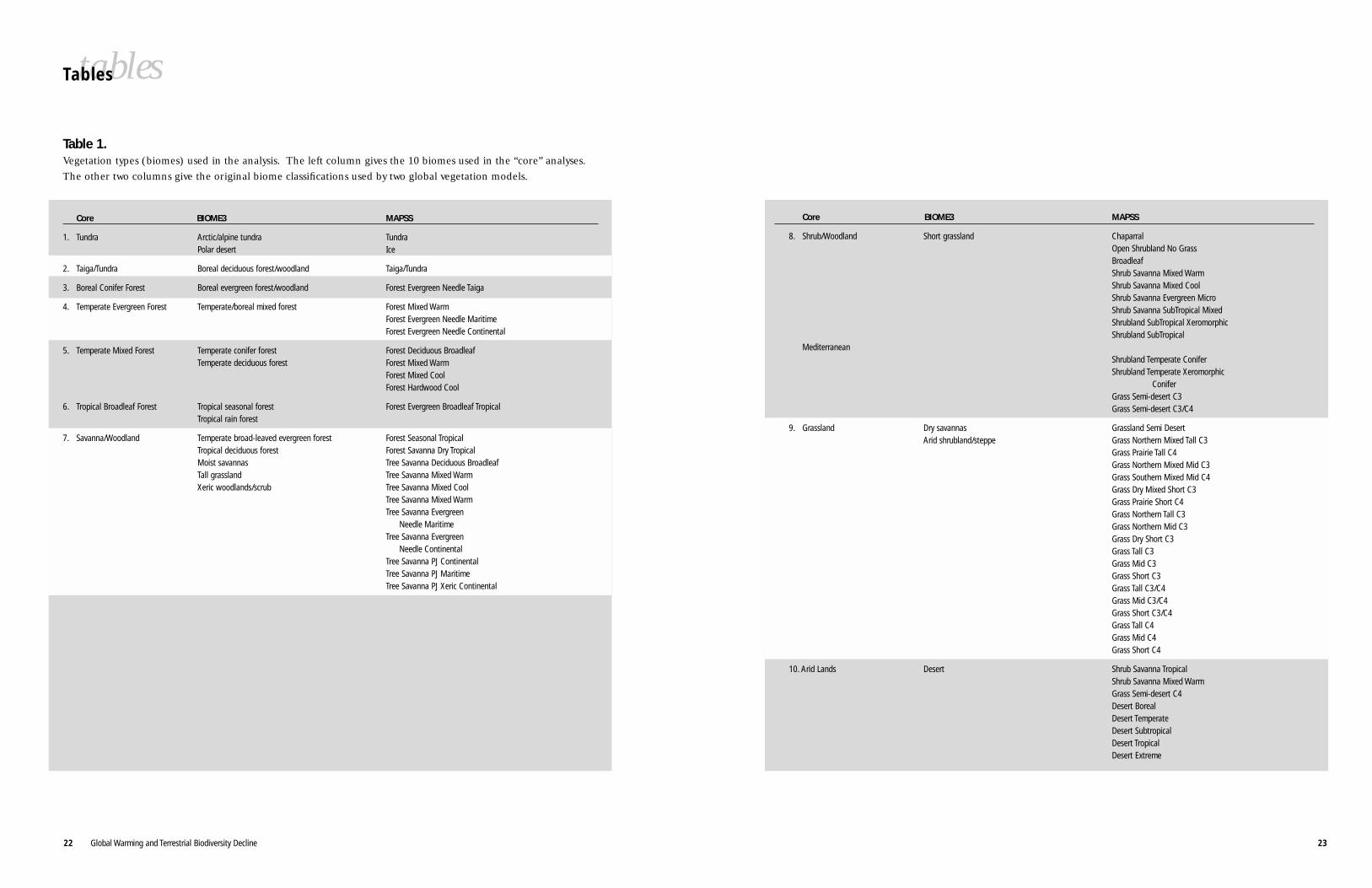
A final important factor to consider is the breadth of the biome definitions. The two vegetation
models used somewhat different definitions of a “biome” and also divided up major biome
types in different ways. Specifically, BIOME3 modeled 18 biome types, whereas MAPSS modeled
45. In general, the use of fewer, more broadly-defined climate envelopes (as in BIOME3) can
be expected to result in lower average migration rates, because existing and future distributions
of a biome will show larger areas of overlap and hence larger areas of zero migration. The use
of fewer biome types is equivalent to assuming that species have relatively large geographic
ranges (and broad habitat requirements). We used a conservative figure, and following Neilson
et al. (1998), in the core calculations used 10 biome types for both models (see Table 1).
Sensitivity Analyses
The variables that we considered in our sensitivity analyses were:
1) Impediments to migration (large water bodies and human land-use change)
2) The time period to attain the doubled CO2 climate
3) The breadth of the biome definitions
The distances that we measured in the core calculations were “crow-fly” distances, i.e., the
shortest straight-line distance between two localities (map grid cell centres). Such distances
ignored potential barriers to migration, such as bodies of water and anthropogenic develop-
ment. To incorporate water barriers, we contrasted the crow-fly distances with distances calcu-
lated using “shortest terrestrial paths.” These consisted of the shortest distances linking centres
of neighbouring terrestrial map cells (including diagonally linked cells). Thus, the calculated
paths were the shortest distances around water bodies5. We also investigated the potential
impact of anthropogenic habitat loss and attendant decreases in migration possibilities by
removing from the shortest path calculations cells that were “highly impacted” by human activ-
ities. These highly impacted cells were assumed to be completely impermeable to migration;
that is, in the shortest path calculations they behaved as though they were water bodies. Our
definition of “highly impacted” was based on model results by Turner (reported in Pitelka et
al. 1997), which suggested that thresholds of movement though fragmented landscapes
occurred when approximately 55% or 85% of habitat was destroyed (respectively, depending
on whether fragmentation was random or aggregated). Simulations by Schwartz (1992) also
indicated shifts in migration rates at close to these values (respectively, depending on whether
resents the observed set of conditions that it actually occupies under the influence of addition-
al factors such as predation, competition, etc. Predicting the effect of global warming on physi-
cal conditions is relatively straightforward, but disentangling the interaction of both physical
and biotic changes is enormously difficult.
Nevertheless we can apply general ecological principles to investigate possible biodiversity
change. In this paper, rather than attempting to model each species, we apply a broader brush
and, as detailed below, take a more heuristic approach. A good example of this sort of
approach is provided by McDonald and Brown (1992) who used empirical species-area rela-
tionships to study biodiversity loss as described above.
Migration rates
The factors affecting the ability of organisms to migrate in response to climate changes are not
well understood even for relatively well-known organisms such as trees. Some studies have
assumed that trees can migrate at most at observed post-glacial rates; however, the validity of this
assumption has been questioned (Clark 1998, Clark et al. 1998). Therefore, instead of attempt-
ing to predict how fast species and biomes might be able to move, we instead asked how fast
might species and biomes be required to move in order to keep up with the projected warming.
As noted above, the climate/vegetation models provided information on the current and
future distributions of major vegetation types. Therefore, we could use the models to calculate
the speeds that biomes might have to achieve in order to keep up with the warming. However,
our primary interest was not in the biomes themselves (a biome is, after all, an abstract entity),
but rather in the species within them. Note however that at least in a heuristic sense, the
movement of the biomes provides indirect information on the movements of species. The
same sorts of physiological variables that the vegetation models use to map biome distributions
are also relevant in mapping the distributions of individual species (especially plant species)
(e.g. Sykes and Prentice 1996). In this sense, the “biome climate envelopes” that the vegeta-
tion models simulate can be thought of as proxies for “species climate envelopes.”
Additionally, species distributions in many cases are strongly associated with particular biome
types; for example, the many plants and animals that can only survive in arctic conditions.
As detailed below, in a series of core calculations we measured required biome migration rates
under a single set of assumptions. To investigate the importance of these assumptions, we also
undertook sensitivity analyses in which they were systematically varied.
Core Calculations
To calculate a migration rate, one divides the migration distance by the time period over
which the migration occurs. To measure distances, we reasoned that the nearest possible immi-
gration source for a locality with future biome type x would be the nearest locality of the same
biome type under the current climate. Thus, the migration distance was calculated as the dis-
tance between a future locality and the nearest same-biome-type locality in the current climate.
For example, the tree shown in Figure 1A in the new habitat patch must have come from an
98 Global Warming and Terrestrial Biodiversity Decline
Migration Rates
Core calculationsSeveral of the differences among the climate and vegetation models influenced biome migra-
tion rates, including the type of vegetation model8, the age of the GCM (older vs. newer gen-
eration models)9, the presence or absence of sulphate cooling10, and the possibility of direct
CO2 effects on plant water use efficiency11. However, all models agreed in that “very high”
migration rates (≥1,000 m/yr) were relatively common, comprising on average 17 and 21% of
the world's surface for the two vegetation models (Figure 2). Migration rates of ≥10,000 m/yr
were rare (<1% of the world's surface).
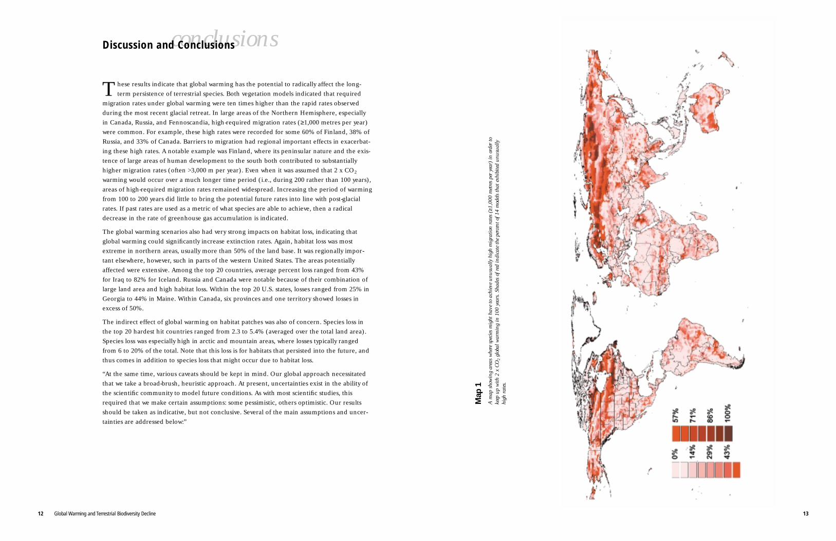
To visually examine the required migration rates, for each grid cell in the world map we plot-
ted the percent of models that exhibited “unusually” high (≥1,000 m/yr) migration rates. We
used 1,000 m/yr as a cut-off point because higher tree migration rates rarely have been
observed in the past (see Clark 1998). High migration rates were consistently observed in the
Northern Hemisphere and included large areas in Canada, Alaska, Russia, Finland, and
Sweden (Map 1). Finland was the hardest hit country overall, with an average of nearly 60% of
the country exhibiting unusually high rates (Table 2). The high percentages observed for
Russia and Canada (respectively 38.3 and 33.1%) are especially notable because of the large
sizes of these countries. Unusually high migration rates were indicated for many large areas in
Canada, with over 40% of their territory with high rates for Ontario, Newfoundland/Labrador,
Quebec, and Manitoba (Table 2). Areas affected in the United States were also substantial,
ranging from 35.7 to 14.7% among the top 20 hardest hit states. Other areas with consistently
high rates included parts of eastern Brazil; Uruguay; eastern Argentina; the savanna/rainforest
border in Africa; southern England; Saudi Arabia; Iraq; India; northeastern China; Thailand;
Cambodia; and southwestern Australia (Map 1). Distinct banding parallelling the orientation
of biome boundaries was evident in several areas, including Canada, Africa, and northern Asia.
These bands reflected the high migration rates required to track the leading edges of pole-
ward-shifting biomes. The high migration rates in the Northern Hemisphere were also evident
when future migration rates were compared among latitudinal classes and vegetation types.
Lowest migrations rates were observed within 20 degrees of the equator, where 6-8% (BIOME3
vegetation model) or 11-13% (MAPSS vegetation model) of map grid cells had migration rates
that exceeded 1,000 m/yr (Figure 3). Average migration rates were nearly constant up to 40
degrees of latitude for BIOME3, but thereafter jumped markedly. The highest migration aver-
age for BIOME3 was in the northernmost latitudinal class (>60 degrees), where 35% of cells
averaged rates ≥1,000 m/yr. The relationship between latitudinal class and average migration
rate was more monotonic for MAPSS than for BIOME3. Maximum migration rates were again
observed in the northernmost latitudinal class for MAPSS and were similar in magnitude to
those observed for BIOME3. Average migration rates for both vegetation models were marked-
ly higher in temperate vegetation types (Taiga/Tundra, Temperate Evergreen Forest,
Temperate Mixed Forest, and Boreal Coniferous Forest) than elsewhere (Figure 4). In these
temperate vegetation types, on average approximately 35% of pixels had rates >1,000 m/yr,
with a maximum of 44% in Temperate Mixed Forest (MAPSS) and a minimum of 27% for
Temperate Evergreen Forest (MAPSS). Average migration rates in the other vegetation
resultsResults
dispersal followed negative exponential or inverse power functions). To quantify habitat
destruction, we made use of the global 1-km unsupervised classification of AVHRR satellite
data undertaken by the United States Geological Service6.
For comparison to the core scenario in which climate change was assumed to occur in 100 years,
we assumed a more conservative time period, namely 200 years. Additionally, we took advantage
of research on post-glacial rates of spruce (Picea) migration (see Pitelka et al. 1997) and com-
pared Picea migration rates against required migration rates calculated for the boreal biome. We
used the boreal biome because the current geographic distribution of Picea in North America is
fairly well approximated by the boreal biome. In the comparisons, we varied the time period of
climate forcing until we achieved maximum agreement between Picea and boreal rates.
Finally, we investigated the relationship between migration rate and biome area by plotting
mean migration rate against biome area for biomes in North America and Africa7. Because
biomes in Africa tended to be distributed into northerly and southerly portions, we calculated
areas and rates separately for the northern and southern portions. This made the African bio-
mes more contiguous and hence more comparable with the North American biomes.
Current Habitat Loss
As shown in Figure 1B, we defined current habitat loss based on areas where current and
future biome types differed. If a grid cell was biome x in the current climate, but became
biome type y in the future climate, then that habitat was assumed to have been lost. As in the
core migration calculations, we used 10 biome types (see Table 1).
Declines in Habitat Patch Area and Associated Species Loss
If species richness is plotted against area on a log-log scale, a more-or-less linear relationship is
typically observed between the two. The slope of the relationship has been observed to vary
systematically under the influence of a variety of factors – for example, slopes in island systems
typically range from 0.24 to 0.33, whereas in continental situations they range from about 0.12
to 0.17 (Pianka 1978). We took a relatively conservative approach and used a value of 0.15. It is
not difficult to show that given some proportion p of habitat remaining, the expected propor-
tion of species remaining is p raised to the power of the slope (0.15 in this case). For example,
an 85% reduction in the area can be expected to result in a 25% reduction in species richness
(see Figure 1C for examples).
To calculate decreases in patch size, first we calculated the areas of patches of contiguous grid
cells of the same biome type under the current climate (these patches included diagonally
linked cells). Second, we calculated the area of the patch that was lost (if any) by determining
which of the original patch cells had changed to a new biome type under the new climate.
Notice that migrations of species into newly-suitable areas may act to partly offset habitat and
species loss (should habitats in the new areas materialize); however, in our calculations we con-
sidered only the effect of the reduction in area.
11
that species with smaller ranges may be more strongly impacted. In comparison to core calcu-
lations, 10% more pixels for BIOME3 and 14% for MAPSS had rates above 316 m/yr. This
increase in migration rates was confirmed when average migration rates was plotted against
biome types for biomes in North America and Africa (Figure 6). As biome area decreased by
an order of magnitude, average BIOME3 migration rates increased by approximately 0.5
orders of magnitude and average MAPSS rates by an order of magnitude. The importance of
latitude in influencing migration rates was evident in that for a given biome area, North
American migration rates were above African ones12.
Habitat Loss
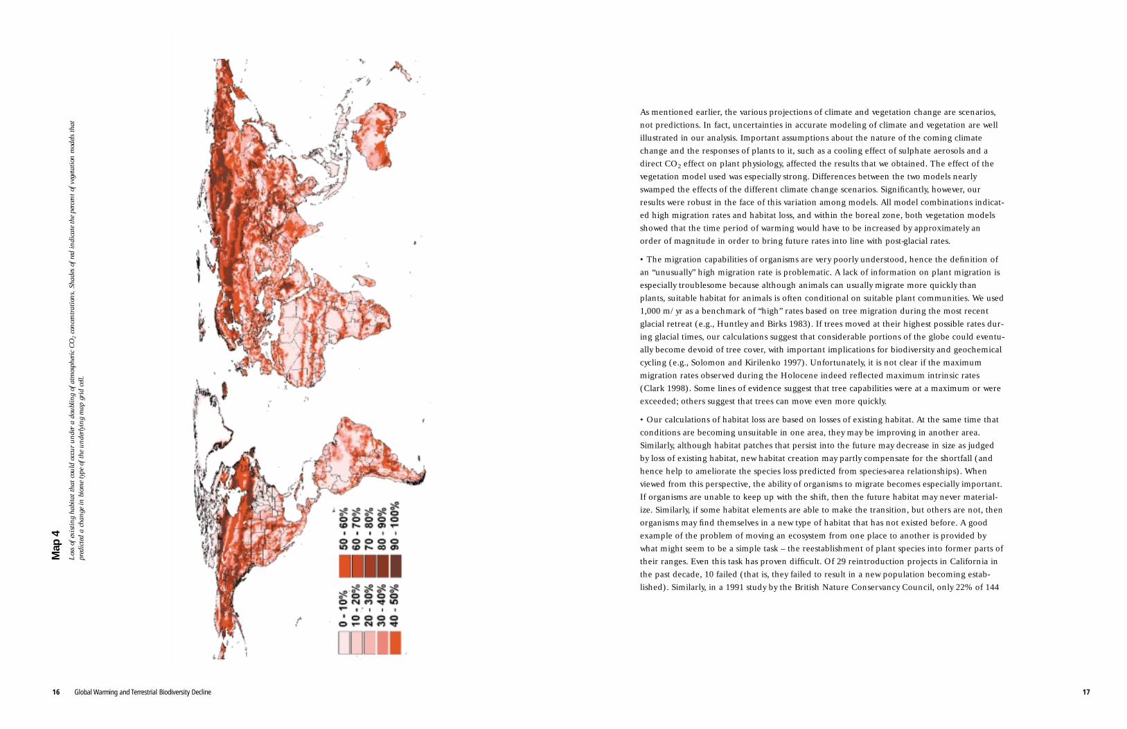
A global map of percentage habitat loss showed a pattern similar to the map of high required
migration rates. Loss of existing habitats was markedly concentrated in the Northern
Hemisphere, especially in Canada, Alaska, Russia, and Fennoscandia (Map 4, Table 5). Other
areas with consistently high loss included parts of the western and south-central United States,
northeastern Saudi Arabia, and parts of Argentina, Australia, China, and Mongolia. Among the
top 20 hardest hit countries, habitat loss was always above 40% (Table 5). Again, because of
their large size, habitat loss was especially notable in Canada and Russia (respectively, 55.8 and
46.3%). More than half of Canadian provinces/territories had greater than 50% habitat loss
and it was especially concentrated along the southern and northern margins of the boreal
zone. Within the United States, the most heavily influenced states were usually in the western
and south-central sections of the country. Among the top 20 states, habitat loss always averaged
greater than 24%.
Averaged over the whole world, habitat loss averaged 35.7% of the land area. For comparison,
habitat already seriously impacted by human activities (as judged by USGS-calculated conver-
sion of 55% of the underlying 1-km pixels) was some 20.1% of the total land area.
Declines in Habitat Patch Area and Associated Species Loss
Species loss associated with decreases in the sizes of habitat patches showed quite a different
spatial pattern (Map 5). Although threats to biodiversity were again concentrated in the
Northern Hemisphere; they tended to occur even further north, into the southern Canadian
Arctic islands and the Taymyr Peninsula of Russia for example. Other concentrations of
species loss included northern Alaska, western Greenland, the northern boreal/taiga zone of
Canada, eastern Argentina, northern Fennoscandia, the Tibetan Plateau of China, and parts of
eastern Siberia (Map 5, Table 6).
10 Global Warming and Terrestrial Biodiversity Decline
(excluding Tundra) tended to be higher for MAPSS than BIOME3. Respectively, an average of
13% and 9% of cells in these remaining vegetation types had rates above 1,000 m/yr. Because
Tundra rarely shifted to new areas, but instead was encroached upon, it had migration rates of
close to zero in both vegetation models.
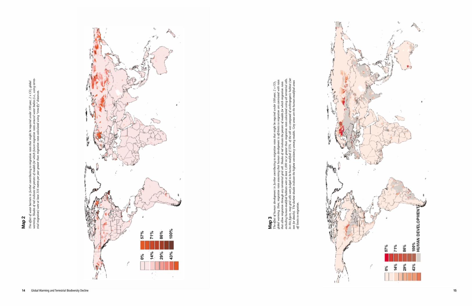
Sensitivity AnalysesBarriers to migration. – Averaged over the whole globe, the migration rates calculated ignoring
water barriers (that is, using “crow-fly” distances) were usually similar to those calculated tak-
ing water barriers in to account (that is, using “shortest-terrestrial-path” distances). Averaged
across all models, 99% of grid cells had shortest-path rates that were within 316 m/yr of their
crow-fly rates (99.1 and 98.9 for BIOME3 and MAPSS respectively; see Table 3). However, the
effect of water as a barrier to migration was often regionally important, especially on islands
(such as Newfoundland) and peninsulas (such as western Finland) (Map 2).
When “human modified” cells were assumed to be off limits to migration, shortest-path migra-
tion rates also changed relatively slightly at the global scale. Compared to shortest-terrestrial-
path distances, the percent of cells that changed their migration rates by 316 m/yr or less
averaged between 97 and 99% for the two vegetation models (Table 3). However, the incorpo-
ration of human barriers was sometimes regionally important. Grid cells with large increases
in migration rates (≥1,000 m/yr) tended to be concentrated along the northern edges of
developed areas in the northern temperate zone, especially in northwestern Russia, Finland,
central Russia and central Canada (Map 3).
The time period of climate change. – Doubling the period of warming from 100 to 200 years
decreased the percentage of cells with very high migration rates (≥1,000 m/yr) by about one
third for BIOME3 (17.4 to 11.8%) and by nearly one half for MAPSS (21.3 to 11.9%) (Table 4).
However, this doubling of the warming period did little to bring required Boreal migration
rates into agreement with rates of spruce (Picea) migration observed during the glacial retreat.
The best fit between Boreal and spruce rates was obtained when the period of warming was
instead increased by approximately an order of magnitude, to 1070 years for BIOME3 and to
1150 years for MAPSS (Figure 5A). At these slower rates of warming, an average of only 1.3% of
nonzero Boreal cells had rates exceeding 1,000 m/yr (Figure 5C). For 100-year warming on the
other hand, percentages of non-zero Boreal cells exceeding 1,000 m/yr averaged 61% for both
BIOME3 and MAPSS (Figure 5B). Therefore, an approximate order of magnitude decrease in
the rate of 2 x CO2 climate change was required in order to bring the two sets of migration
rates into agreement. On a more positive note, however, improvement in the rate of fit between
the two sets was most rapid for slight increases in the time period. Thus, slight decreases in the
rate of warming had a disproportionate effect in reducing required migration rates.
Number of biome types. – As expected, use of more biomes types (18 for BIOME3 and 45 for
MAPSS) yielded higher average migration rates than when only 10 types were used, indicating
1312 Global Warming and Terrestrial Biodiversity Decline
conclusionsDiscussion and Conclusions
These results indicate that global warming has the potential to radically affect the long-
term persistence of terrestrial species. Both vegetation models indicated that required
migration rates under global warming were ten times higher than the rapid rates observed
during the most recent glacial retreat. In large areas of the Northern Hemisphere, especially
in Canada, Russia, and Fennoscandia, high-required migration rates (≥1,000 metres per year)
were common. For example, these high rates were recorded for some 60% of Finland, 38% of
Russia, and 33% of Canada. Barriers to migration had regional important effects in exacerbat-
ing these high rates. A notable example was Finland, where its peninsular nature and the exis-
tence of large areas of human development to the south both contributed to substantially
higher migration rates (often >3,000 m per year). Even when it was assumed that 2 x CO2
warming would occur over a much longer time period (i.e., during 200 rather than 100 years),
areas of high-required migration rates remained widespread. Increasing the period of warming
from 100 to 200 years did little to bring the potential future rates into line with post-glacial
rates. If past rates are used as a metric of what species are able to achieve, then a radical
decrease in the rate of greenhouse gas accumulation is indicated.
The global warming scenarios also had very strong impacts on habitat loss, indicating that
global warming could significantly increase extinction rates. Again, habitat loss was most
extreme in northern areas, usually more than 50% of the land base. It was regionally impor-
tant elsewhere, however, such in parts of the western United States. The areas potentially
affected were extensive. Among the top 20 countries, average percent loss ranged from 43%
for Iraq to 82% for Iceland. Russia and Canada were notable because of their combination of
large land area and high habitat loss. Within the top 20 U.S. states, losses ranged from 25% in
Georgia to 44% in Maine. Within Canada, six provinces and one territory showed losses in
excess of 50%.
The indirect effect of global warming on habitat patches was also of concern. Species loss in
the top 20 hardest hit countries ranged from 2.3 to 5.4% (averaged over the total land area).
Species loss was especially high in arctic and mountain areas, where losses typically ranged
from 6 to 20% of the total. Note that this loss is for habitats that persisted into the future, and
thus comes in addition to species loss that might occur due to habitat loss.
“At the same time, various caveats should be kept in mind. Our global approach necessitated
that we take a broad-brush, heuristic approach. At present, uncertainties exist in the ability of
the scientific community to model future conditions. As with most scientific studies, this
required that we make certain assumptions: some pessimistic, others optimistic. Our results
should be taken as indicative, but not conclusive. Several of the main assumptions and uncer-
tainties are addressed below:”
Map
1A
map
sho
win
g ar
eas
whe
re s
peci
es m
ight
hav
e to
ach
ieve
unu
sual
ly h
igh
mig
ratio
n ra
tes
(≥1,
000
met
res
per
year
) in
ord
er to
keep
up
with
2 x
CO
2gl
obal
war
min
g in
100
yea
rs. S
hade
s of
red
indi
cate
the
perc
ent o
f 14
mod
els
that
exh
ibite
d un
usua
llyhi
gh r
ates
.
1514 Global Warming and Terrestrial Biodiversity Decline
Map
2T
he e
ffect
of w
ater
bar
rier
s in
furt
her
cont
ribu
ting
to m
igra
tion
rate
s th
at m
ight
be
requ
ired
und
er 1
00-y
ear,
2 x
CO
2gl
obal
war
min
g. S
hade
s of
red
indi
cate
the
perc
ent o
f mod
els
for
whi
ch fu
ture
mig
ratio
n ra
tes
arou
nd w
ater
bod
ies
(i.e
., us
ing
terr
es-
tria
l mig
ratio
n) w
ere
at le
ast 3
16 m
etre
s pe
r ye
ar g
reat
er th
an m
igra
tion
rate
s ca
lcul
ated
usi
ng “
crow
-fly”
dis
tanc
es.
Map
3
The
effe
ct o
f hum
an d
evel
opm
ent i
n fu
rthe
r co
ntri
butin
g to
mig
ratio
n ra
tes
that
mig
ht b
e re
quir
ed u
nder
100
-yea
r, 2
x C
O2
glob
al w
arm
ing.
Her
e, m
igra
tion
rate
s as
sum
ing
that
hum
an d
evel
opm
ent i
s of
f-lim
its to
mig
ratio
n ar
e co
ntra
sted
with
rat
esth
at a
llow
mig
ratio
n th
roug
h an
y te
rres
tria
l gri
d ce
ll. S
hade
s of
red
indi
cate
the
perc
ent o
f mod
els
for
whi
ch m
igra
tion
rate
sex
clud
ing
hum
an-m
odifi
ed h
abita
ts w
ere
at le
ast 1
,000
m/y
r gr
eate
r th
an m
igra
tion
rate
s ca
lcul
ated
usi
ng a
ll te
rres
tria
l cel
ls.
In th
is fi
gure
, map
gri
d ce
lls w
ere
judg
ed to
be
hum
an m
odifi
ed if
55%
of t
he c
ell w
as c
ompo
sed
of a
nthr
opog
enic
hab
itat (
see
text
for
deta
ils).
The
dar
kest
sha
des
indi
cate
the
high
est c
onsi
sten
cy a
mon
g m
odel
s. G
rey
area
s ar
e th
e hu
man
-mod
ified
are
asof
f lim
its to
mig
ratio
n.
16 Global Warming and Terrestrial Biodiversity Decline 17
As mentioned earlier, the various projections of climate and vegetation change are scenarios,
not predictions. In fact, uncertainties in accurate modeling of climate and vegetation are well
illustrated in our analysis. Important assumptions about the nature of the coming climate
change and the responses of plants to it, such as a cooling effect of sulphate aerosols and a
direct CO2 effect on plant physiology, affected the results that we obtained. The effect of the
vegetation model used was especially strong. Differences between the two models nearly
swamped the effects of the different climate change scenarios. Significantly, however, our
results were robust in the face of this variation among models. All model combinations indicat-
ed high migration rates and habitat loss, and within the boreal zone, both vegetation models
showed that the time period of warming would have to be increased by approximately an
order of magnitude in order to bring future rates into line with post-glacial rates.
• The migration capabilities of organisms are very poorly understood, hence the definition of
an “unusually” high migration rate is problematic. A lack of information on plant migration is
especially troublesome because although animals can usually migrate more quickly than
plants, suitable habitat for animals is often conditional on suitable plant communities. We used
1,000 m/yr as a benchmark of “high” rates based on tree migration during the most recent
glacial retreat (e.g., Huntley and Birks 1983). If trees moved at their highest possible rates dur-
ing glacial times, our calculations suggest that considerable portions of the globe could eventu-
ally become devoid of tree cover, with important implications for biodiversity and geochemical
cycling (e.g., Solomon and Kirilenko 1997). Unfortunately, it is not clear if the maximum
migration rates observed during the Holocene indeed reflected maximum intrinsic rates
(Clark 1998). Some lines of evidence suggest that tree capabilities were at a maximum or were
exceeded; others suggest that trees can move even more quickly.
• Our calculations of habitat loss are based on losses of existing habitat. At the same time that
conditions are becoming unsuitable in one area, they may be improving in another area.
Similarly, although habitat patches that persist into the future may decrease in size as judged
by loss of existing habitat, new habitat creation may partly compensate for the shortfall (and
hence help to ameliorate the species loss predicted from species-area relationships). When
viewed from this perspective, the ability of organisms to migrate becomes especially important.
If organisms are unable to keep up with the shift, then the future habitat may never material-
ize. Similarly, if some habitat elements are able to make the transition, but others are not, then
organisms may find themselves in a new type of habitat that has not existed before. A good
example of the problem of moving an ecosystem from one place to another is provided by
what might seem to be a simple task – the reestablishment of plant species into former parts of
their ranges. Even this task has proven difficult. Of 29 reintroduction projects in California in
the past decade, 10 failed (that is, they failed to result in a new population becoming estab-
lished). Similarly, in a 1991 study by the British Nature Conservancy Council, only 22% of 144
Map
4L
oss
of e
xist
ing
habi
tat t
hat c
ould
occ
ur u
nder
a d
oubl
ing
of a
tmos
pher
ic C
O2
conc
entr
atio
ns. S
hade
s of
red
indi
cate
the
perc
ent o
f veg
etat
ion
mod
els
that
pred
icte
d a
chan
ge in
bio
me
type
of t
he u
nder
lyin
g m
ap g
rid
cell.
1918 Global Warming and Terrestrial Biodiversity Decline
dant. This is an important concern for many plant species; for example, the Nature
Conservancy estimates that one-half of endangered plant taxa in the U.S. are restricted to five
or fewer populations (from Pitelka et al. 1997). Schwartz (1992, see also Davis 1989) also
noted that climate warming also could especially threaten species with geographically restrict-
ed ranges (such as narrow endemics), those restricted to habitat islands, and specialists on
uncommon habitats. Thus, the potential for attaining the high-required rates observed here
may be even lower for species that are rare in their range.
• In our investigation of migration rates and habitat loss, we did not consider the magnitude
of the local climate change. In some areas, new established climatic conditions may differ sub-
stantially from preexisting conditions, whereas in other areas, the changes may be less
extreme. More extreme change will more quickly reduce the available time for migration and
hence possibilities for establishment of new habitat.
• Finally, migration through human modified habitats was treated as an all-or-none process in
very large grid cells (0.5 degrees of latitude/longitude). This meant that only relatively exten-
sively developed areas were excluded from migration and that diffusion processes present at
small spatial scales were lost (see Dyer 1995). The use of the U.S. Geological Service classifica-
tion also led to a strong emphasis on agricultural development. Other less intensive forms of
development were ignored. For example, Schwartz (1992) noted that compared to the original
primary forest, the secondary forests of the northeastern U.S. were of uneven quality, which
may influence colonization by slowgrowing shade tolerant trees and exacerbate differences in
migration rates among species.
Despite these uncertainties, the magnitude of the effects reported here are of great concern
from a biodiversity perspective. Based on existing knowledge, it appears safe to conclude that
although some plants will be able to keep up with the rates reported here, others will not.
These rates seem unlikely to pose a problem for invasive species and others with high dispersal
capabilities, which have migrational capabilities that may typically exceed 1,000 m/yr. For
example, Weber (1998) found that when two goldenrod species (Soldago spp.) invaded
Europe, range diameters increased from 400 to 1400 km between 1850 and 1875 and from
1400 to 1800 km between 1875 and 1990 (see his Figure 3). Assuming a circular range
expanding constantly outward, respective migration rates were approximately 20,000 and
1,740 m/yr. Similarly, after its arrival in western North America in about 1880, in approximate-
ly 40 years cheatgrass had occupied most of its range of 200,000 km2 (Mack 1986). Again
assuming a circular range, a 40-year period to traverse the radius gives a migration rate of
6,300 m/yr. Animals are presumably able to migrate faster than plants (Davis 1986); for exam-
ple, water beetles appeared in deglaciated areas long before trees (Morgan et al. 1983).
However, as noted above, successful establishment by many animal species may ultimately
depend on appropriate floristic and/or structural habitat features.
species reintroductions were deemed successful and more than half appeared to have failed.
Successful reestablishment of functioning ecosystems, which might include establishment of
self-sustaining populations, pollinators, mycorrhizal fungi, seed dispensers, nutrient cycles, and
hydrology, is much less likely (Allen 1994). Certainly, nature will do a better job than humans
will, but this example demonstrates the potential problems of moving an ecosystem from one
place to another.
• These results pertain only to a doubling of carbon dioxide concentrations. Should atmos-
pheric concentrations rise even higher, and hence cause even more extreme warming, greater
loss of existing habitat and reductions in patch area would be expected.
• Our scenarios of migration rates and our conclusions about species loss through loss of exist-
ing habitat failed to consider outlier populations. We used sharp biome boundaries and hence
implicitly assumed sharp boundaries of species distributions. In fact, species are often found in
outlier populations, which can contribute to more rapid migration than along a single popula-
tion front because of rapid in-filling between populations (Davis et al. 1991, Pitelka et al. 1997,
Clark 1998). As noted by Davis (1986), plants continue to compete tenaciously for space even
in the face of changed conditions and relictual populations can survive for many years in the
absence of flowering and seed set. Although trees and perennials are at a disadvantage with
respect to rapidly shifting climate envelopes because of slow maturity and low reproductive
rates (Pitelka et al. 1997), these same factors may promote the maintenance of outlier popula-
tions that can serve as sources of colonists. These relictual populations also significantly
decrease the likelihood of global extinction vs. local extinction. They become especially signifi-
cant if conditions improve, allowing a species to potentially re-colonize former parts of its
range. This importance of outlier populations reinforces the important conservation value of
populations that are “outside” of their usual range.
• The potential existence of outlier populations argues for the use of relatively liberal esti-
mates of range sizes in estimating climatically induced migration rates. If a species occurs in
only a subset of its climatically possible range, but climate is nonetheless used to model its
actual distribution, then estimated climate-induced migration distances will be erroneously
high. By defining only 10 biome types, our core calculations implicitly assumed relatively large
range sizes and hence provided relatively conservative migration rates. As expected, we found
that as the size of modeled distributions decreased, required migration rates increased, albeit
not strikingly across the range of sizes that we investigated. Required migration rates may be
higher for species with smaller range sizes.
• An important factor relevant to the conservation of rare taxa was our failure to incorporate
possible density dependent effects. For example, Schwartz's (1992) simulations showed that
rare species never attained their highest migration rates even when suitable habitat was abun-
tude of this winnowing effect is unknown. Some evidence suggests that post-glacial migration
limitation has similarly resulted in a subset of highly mobile taxa. If so, given that global warm-
ing might require much higher migration rates, it can be expected to result in even greater
species loss, especially in nonglaciated areas that previously have not undergone any selection
for high mobility taxa. The possibility of high rates of climate change in tropical areas is of
particular concern given the presumed importance of long-term climatic stability in contribut-
ing to high species diversity and the possibility of much lower intrinsic rates of migration than
in the temperate zone.
In conclusion, future migration rates due to global warming may be unprecedented even
when judged against rapid post-glacial migration rates. Although migration capabilities are
poorly known, it seems likely that these rates will be beyond the capabilities of many species,
and will lead to a reduction in biodiversity. Without suitable migration, global warming has the
potential to destroy large areas of habitat. For cold-adapted systems, such as arctic and alpine
systems, global warming will impose species loss quite irrespective of migrational capabilities.
Increases in connectivity among natural habitats within developed landscapes may help organ-
isms to attain their maximum intrinsic rates of migration. However, in order to bring future
migration rates into line with even the rapid migration rates of the past, it is apparent that
large and rapid reductions in greenhouse gas emissions are required.
2120 Global Warming and Terrestrial Biodiversity Decline
For many other plant species, however, these rates will likely pose a problem. Aside from setting
a possible upper bound on plant migration capabilities, migration rates for invasive species are
probably of limited relevance for many plant species. Invasive species often have abnormally
high fecundity and dispersal capabilities and in many cases their migration is aided by humans.
Troubling information comes from field studies of reinvasions by forest herbs into previously
plowed secondary forests. Both Matlack (1994) and Brunet and Von Oheimb (1998) found that
distance to oldgrowth was a correlate of understory richness in the successional stands, suggest-
ing migration limitation. Matlack (1994) found no measurable movement for some species and
only a small subset (<10% of 51) showed rates as high as 2-3 m/yr. Similarly, Brunet and
Oheimb (1998) reported a median migration rate of only 0.3 m/yr (49 species). Other studies
(cited in Matlack 1994) have also reported extremely slow movement of forest herbs. At the
opposite end of the spectrum from invasive species are species that have evolved in situ and
might fail to migrate at all. As Brunet and Von Oheimb (1998) pointed out, even though the
understory flora appeared to be migrating very slowly, it had evidently migrated into southern
Sweden from remote refugia during the last glaciation and therefore had shown much higher
migration rates in the past. They suggested that compared to past migration, contemporary
migration was limited by such factors such as seed predation, availability of suitable microsites,
and vigour of clonal growth. Presumably, the newly-opened colonization sites exposed by the
glacier would have presented a very different, and presumably more favourable, environment
for migrating species compared to today’s already established communities (Dyer 1995). In the
absence of significant disturbance, many plant communities, especially forested ones, are quite
resistant to invasion, and community-level changes may be delayed for many decades (Pitelka et
al. 1997). For example, forest communities modeled by Davis and Botkin (1985) showed 100-
200 year timelags in the replacement of dominant species, even though seedlings were available
for all species throughout the experiment.
If some species are able to attain the high rates revealed here, whereas others are not, then
global warming can be expected to have a “filtering” or “winnowing” effect on plant communi-
ties. Matlack (1994) noted that just as agricultural development has put a premium on long-
range dispersal of plants, resulting in the selection a recognizable “old-field” flora preadapted
to human disturbance, the same mechanism appeared to have selected a high-mobility flora in
the successional forest he studied. Global warming is another factor than may result in a
“weedier” future, resulting in a subset of plant species comprised of highly mobile species
(Sykes and Prentice 1996, Walker and Steffen 1997). Unfortunately, no attempts have been
made to characterize the migration capabilities of entire plant communities, hence the magni-
2322 Global Warming and Terrestrial Biodiversity Decline
tablesTables
Table 1.Vegetation types (biomes) used in the analysis. The left column gives the 10 biomes used in the “core” analyses.
The other two columns give the original biome classifications used by two global vegetation models.
Core BIOME3 MAPSS
1. Tundra Arctic/alpine tundra TundraPolar desert Ice
2. Taiga/Tundra Boreal deciduous forest/woodland Taiga/Tundra
3. Boreal Conifer Forest Boreal evergreen forest/woodland Forest Evergreen Needle Taiga
4. Temperate Evergreen Forest Temperate/boreal mixed forest Forest Mixed Warm Forest Evergreen Needle MaritimeForest Evergreen Needle Continental
5. Temperate Mixed Forest Temperate conifer forest Forest Deciduous BroadleafTemperate deciduous forest Forest Mixed Warm
Forest Mixed CoolForest Hardwood Cool
6. Tropical Broadleaf Forest Tropical seasonal forest Forest Evergreen Broadleaf TropicalTropical rain forest
7. Savanna/Woodland Temperate broad-leaved evergreen forest Forest Seasonal TropicalTropical deciduous forest Forest Savanna Dry TropicalMoist savannas Tree Savanna Deciduous BroadleafTall grassland Tree Savanna Mixed WarmXeric woodlands/scrub Tree Savanna Mixed Cool
Tree Savanna Mixed WarmTree Savanna Evergreen
Needle MaritimeTree Savanna Evergreen
Needle ContinentalTree Savanna PJ ContinentalTree Savanna PJ MaritimeTree Savanna PJ Xeric Continental
Core BIOME3 MAPSS
8. Shrub/Woodland Short grassland ChaparralOpen Shrubland No GrassBroadleafShrub Savanna Mixed WarmShrub Savanna Mixed Cool Shrub Savanna Evergreen MicroShrub Savanna SubTropical MixedShrubland SubTropical XeromorphicShrubland SubTropical
MediterraneanShrubland Temperate ConiferShrubland Temperate Xeromorphic
ConiferGrass Semi-desert C3Grass Semi-desert C3/C4
9. Grassland Dry savannas Grassland Semi DesertArid shrubland/steppe Grass Northern Mixed Tall C3
Grass Prairie Tall C4Grass Northern Mixed Mid C3Grass Southern Mixed Mid C4Grass Dry Mixed Short C3Grass Prairie Short C4Grass Northern Tall C3Grass Northern Mid C3Grass Dry Short C3Grass Tall C3Grass Mid C3Grass Short C3Grass Tall C3/C4Grass Mid C3/C4Grass Short C3/C4Grass Tall C4Grass Mid C4Grass Short C4
10. Arid Lands Desert Shrub Savanna Tropical Shrub Savanna Mixed Warm Grass Semi-desert C4Desert BorealDesert TemperateDesert SubtropicalDesert TropicalDesert Extreme

2524 Global Warming and Terrestrial Biodiversity Decline
Table 2.Countries, U.S. states, and Canadian provinces ranked according to the percent of their territory with unusually high
required migration rates (≥1,000 m/yr). Only the first 20 countries and states are shown. Countries had to occupy at
least 5 grid cells to be included in the table.
A. Country Grid Cell Count Percent1
Finland 249 59.9Uruguay 70 43.9Kuwait 8 41.1Russia 11539 38.3Estonia 26 34.9Iceland 63 34.6Sweden 309 34.4Canada 6228 33.1Cuba 38 32.1Latvia 35 31.0Thailand 171 30.0Burkina Faso 86 30.0United Kingdom 131 29.8Portugal 39 29.5Benin 39 28.8Cambodia 62 27.9Taiwan 13 27.5Bangladesh 47 27.2Ireland 38 26.3Dominican Republic 15 26.2
1Averaged across 14 combinations of global climate and vegeta-tion models.
B. U.S. State Grid Cell Count Percent1
Maryland 7 35.7Tennessee 41 31.9Utah 92 28.3Kansas 88 27.8Delaware 3 26.2Louisiana 43 25.6Vermont 14 23.0Arkansas 55 22.5Oklahoma 71 22.4Wyoming 112 21.6Maine 37 20.1Arizona 113 19.3Colorado 112 17.3Idaho 96 16.1New Hampshire 12 16.1New Jersey 9 15.9New York 56 15.3Nebraska 86 14.9Mississippi 47 14.7Alabama 51 14.7
C. Canadian Provinceor Territory Grid Cell Count Percent1
Ontario 500 49.2Newfoundland 203 48.3and LabradorQuebec 857 47.0Manitoba 355 43.0Alberta 375 33.3Yukon Territory 341 31.8Nova Scotia 24 29.2Northwest Territories 2699 25.9British Columbia 542 25.5Saskatchewan 356 24.8Prince Edward Island 3 11.9New Brunswick 38 10.9
Table 3.Increases in required migration rates for: 1) migration that went around water (rather than by straight "crow-fly dis-
tances") and 2) migration that went around human development (rather than just around water). For the latter, two
anthropogenic habitat loss scenarios were assumed, 55 or 85% (see text). Values are mean (_ SEM) percent of grid
cells in the various classes of migration rate increases.
Table 4.Mean (_ SEM) percent of grid cells in six migration rate classes for the two global vegetation models and for assump-
tions about the time period during which warming under a 2 x CO2 atmosphere might be achieved (100 and 200
years). Sample size (n) is the number of climate models used for each vegetation model.
Shortest-path plus 55% Shortest-path plus 85% Shortest-path habitat loss habitat loss
Increase class BIOME3 MAPSS BIOME3 MAPSS BIOME3 MAPSS(m/yr) (n = 6) (n = 8) (n = 6) (n = 8) (n = 6) (n = 8)0-<316 99.1 ± 0.075 98.9 ± 0.181 97.6 ± 0.346 97.0 ± 0.288 99.1 ± 0.146 98.0 ± 0.176316-<1,000 0.65 ± 0.055 0.63 ± 0.084 1.32 ± 0.199 1.06 ± 0.092 0.53 ± 0.072 0.90 ± 0.0591,000-<3,162 0.12 ± 0.025 0.21 ± 0.046 0.50 ± 0.075 0.74 ± 0.107 0.25 ± 0.049 0.76 ± 0.1023,162-<10,000 0.05 ± 0.002 0.13 ± 0.028 0.28 ± 0.083 0.82 ± 0.073 0.13 ± 0.029 0.17 ± 0.00810,000-<31,622 0.02 ± 0.002 0.08 ± 0.011 0.08 ± 0.016 0.06 ± 0.010 0.01 ± 0.002 0.01 ± 0.00231,622-100,000 – 0.001 ± 0.0005 – – – –Undefined1 0.08 ± 0.016 0.041 ± 0.005 0.19 ± 0.022 0.30 ± 0.025 0.08 ± 0.008 0.13 ± 0.016
1 Cells for which there was no path to a 1 x CO2 cell of the same biome type.
BIOME3 (n = 6) MAPSS (n = 8)Migration rate class (m/yr) 100-yr warming 200-yr warming 100-yr warming 200-yr warming
0-<316 71.1 ± 1.23 79.6 ± 1.11 61.0 ± 1.75 73.7 ± 1.86316-<1,000 11.6 ± 0.26 9.6 ± 0.45 17.7 ± 0.10 14.4 ± 0.331,000-<3,162 10.6 ± 0.53 8.8 ± 0.52 13.9 ± 0.57 9.3 ± 0.873,162-<10,000 5.9 ± 0.57 1.9 ± 0.43 6.6 ± 1.05 2.5 ± 0.6610,000-<31,622 0.9 ± 0.18 0.1 ± 0.03 0.6 ± 0.22 0.09 ± 0.0431,622-100,000 0.03 ± 0.008 0.01 ± 0.006 0.03 ± 0.02 0.004 ± 0.0005
2726 Global Warming and Terrestrial Biodiversity Decline
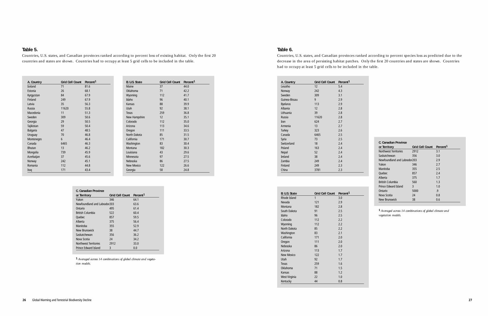
Table 5.Countries, U.S. states, and Canadian provinces ranked according to percent loss of existing habitat. Only the first 20
countries and states are shown. Countries had to occupy at least 5 grid cells to be included in the table.
A. Country Grid Cell Count Percent1
Iceland 71 81.6Estonia 26 68.1Kyrgyzstan 84 67.9Finland 249 67.9Latvia 35 56.3Russia 11620 55.8Macedonia 11 51.3Sweden 309 50.6Georgia 29 50.5Tajikistan 59 50.4Bulgaria 47 48.5Uruguay 70 46.8Montenegro 6 46.4Canada 6465 46.3Bhutan 13 46.2Mongolia 739 45.9Azerbaijan 37 45.6Norway 242 45.1Romania 112 44.8Iraq 171 43.4
B. U.S. State Grid Cell Count Percent1
Maine 37 44.0Oklahoma 71 42.2Wyoming 112 41.7Idaho 96 40.1Kansas 88 39.9Utah 92 38.1Texas 259 36.8New Hampshire 12 35.1Colorado 112 35.0Arizona 113 34.6Oregon 111 33.5North Dakota 85 31.5California 171 30.7Washington 83 30.4Montana 182 30.3Louisiana 43 29.6Minnesota 97 27.5Nebraska 86 27.5New Mexico 122 26.6Georgia 58 24.8
C. Canadian Province or Territory Grid Cell Count Percent1
Yukon 346 64.1Newfoundland and Labrador203 63.6Ontario 495 61.4British Columbia 522 60.4Quebec 857 59.5Alberta 375 56.4Manitoba 355 52.9New Brunswick 38 44.7Saskatchewan 356 36.2Nova Scotia 24 34.2Northwest Territories 2912 33.0Prince Edward Island 3 0.0
1 Averaged across 14 combinations of global climate and vegeta-tion models.
Table 6.Countries, U.S. states, and Canadian provinces ranked according to percent species loss as predicted due to the
decrease in the area of persisting habitat patches. Only the first 20 countries and states are shown. Countries
had to occupy at least 5 grid cells to be included in the table.
A. Country Grid Cell Count Percent1
Lesotho 12 5.4Norway 242 4.3Sweden 309 3.1Guinea-Bissau 9 2.9Byelarus 113 2.9Albania 12 2.8Lithuania 39 2.8Russia 11620 2.8Iran 624 2.7Armenia 13 2.7Turkey 323 2.6Canada 6465 2.5Syria 73 2.5Switzerland 18 2.4Poland 163 2.4Nepal 52 2.4Ireland 38 2.4Zambia 249 2.4Finland 249 2.3China 3781 2.3
C. Canadian Provinceor Territory Grid Cell Count Percent1
Northwest Territories 2912 3.1Saskatchewan 356 3.0Newfoundland and Labrador203 2.9Yukon 346 2.7Manitoba 355 2.5Quebec 857 2.4Alberta 375 1.7British Columbia 560 1.3Prince Edward Island 3 1.0Ontario 5000 .9Nova Scotia 24 0.8New Brunswick 38 0.6
1 Averaged across 14 combinations of global climate and vegetation models.
B. U.S. State Grid Cell Count Percent1
Rhode Island 1 3.0Nevada 121 2.9Montana 182 2.8South Dakota 91 2.5Idaho 96 2.5Colorado 112 2.2Wyoming 112 2.2North Dakota 85 2.2Washington 83 2.1California 171 2.0Oregon 111 2.0Nebraska 86 2.0Arizona 113 1.7New Mexico 122 1.7Utah 92 1.7Texas 259 1.6Oklahoma 71 1.5Kansas 88 1.2West Virginia 22 1.0Kentucky 44 0.8
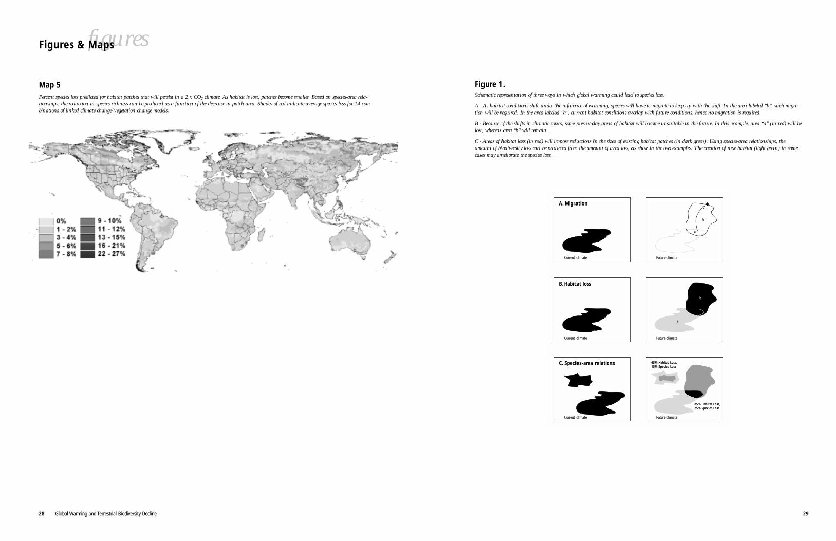
2928 Global Warming and Terrestrial Biodiversity Decline
A. Migration
Current climate Future climate
B. Habitat loss
Current climate Future climate
C. Species-area relations
Current climate Future climate
65% Habitat Loss,15% Species Loss
85% Habitat Loss,25% Species Loss
a
b
a
b
Figure 1.Schematic representation of three ways in which global warming could lead to species loss.
A - As habitat conditions shift under the influence of warming, species will have to migrate to keep up with the shift. In the area labeled “b”, such migra-tion will be required. In the area labeled “a”, current habitat conditions overlap with future conditions, hence no migration is required.
B - Because of the shifts in climatic zones, some present-day areas of habitat will become unsuitable in the future. In this example, area “a” (in red) will belost, whereas area “b” will remain.
C - Areas of habitat loss (in red) will impose reductions in the sizes of existing habitat patches (in dark green). Using species-area relationships, theamount of biodiversity loss can be predicted from the amount of area loss, as show in the two examples. The creation of new habitat (light green) in somecases may ameliorate the species loss.
figuresFigures & Maps
Map 5Percent species loss predicted for habitat patches that will persist in a 2 x CO2 climate. As habitat is lost, patches become smaller. Based on species-area rela-tionships, the reduction in species richness can be predicted as a function of the decrease in patch area. Shades of red indicate average species loss for 14 com-binations of linked climate change/vegetation change models.
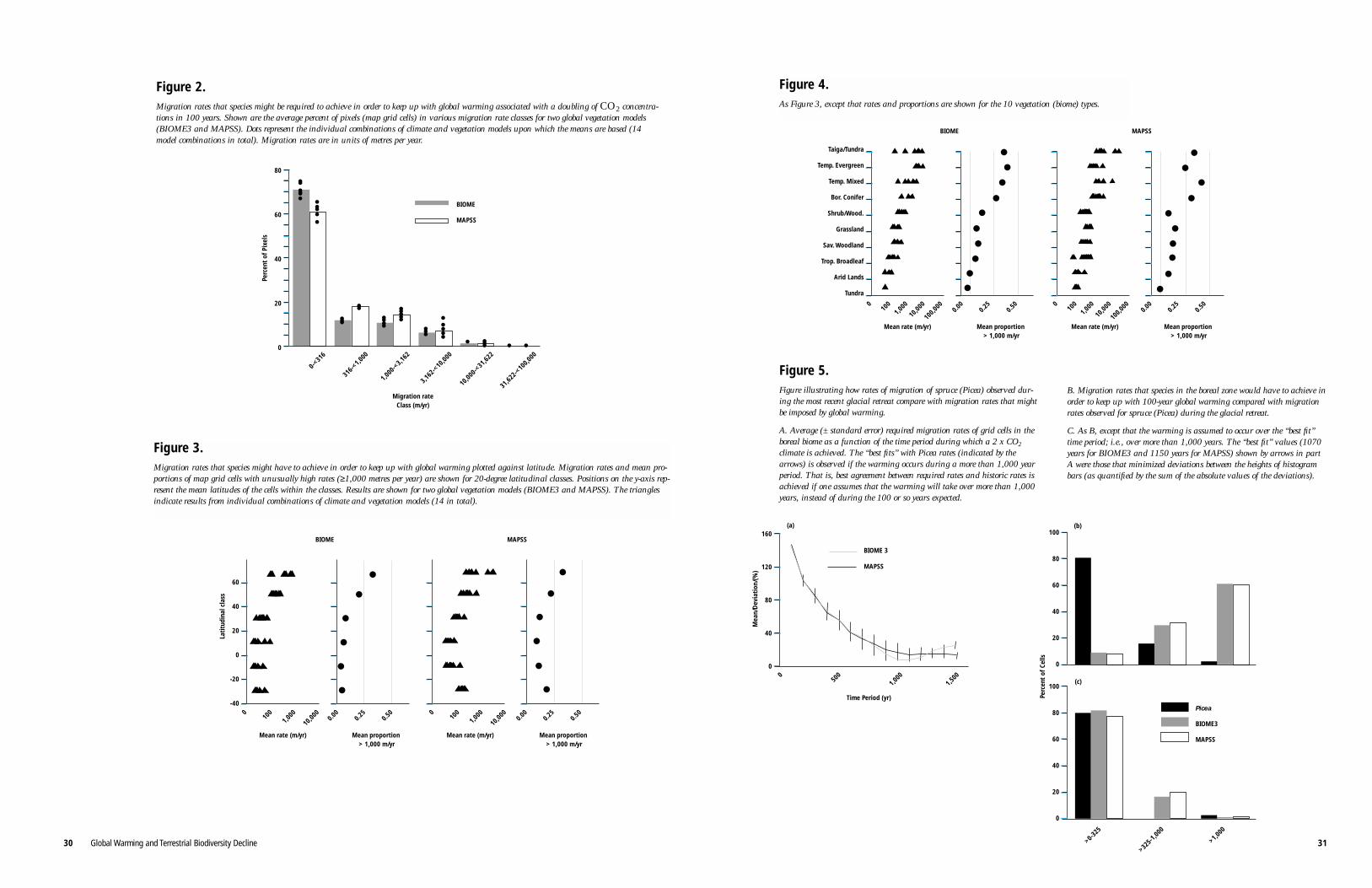
3130 Global Warming and Terrestrial Biodiversity Decline
60
40
20
0
-20
-40
0
10,00
0
100
1,000 0
0.00
0.25
0.50
0.00
0.25
0.50
10,00
0
100
1,000
BIOME MAPSS
Lati
tudi
nal c
lass
Mean rate (m/yr) Mean proportion > 1,000 m/yr
Mean rate (m/yr) Mean proportion > 1,000 m/yr
••••
••
•••••
•
Taiga/Tundra
Temp. Evergreen
Temp. Mixed
Bor. Conifer
Shrub/Wood.
Grassland
Sav. Woodland
Trop. Broadleaf
Arid Lands
Tundra
0
1,000100
10,00
010
0,000 0
1,000100
10,00
010
0,0000.00
0.25
0.50
0.00
0.25
0.50
BIOME MAPSS
Mean rate (m/yr) Mean proportion > 1,000 m/yr
Mean rate (m/yr) Mean proportion > 1,000 m/yr
••
••
•••••
•
•••
•••••••
Figure 3.Migration rates that species might have to achieve in order to keep up with global warming plotted against latitude. Migration rates and mean pro-portions of map grid cells with unusually high rates (≥1,000 metres per year) are shown for 20-degree latitudinal classes. Positions on the y-axis rep-resent the mean latitudes of the cells within the classes. Results are shown for two global vegetation models (BIOME3 and MAPSS). The trianglesindicate results from individual combinations of climate and vegetation models (14 in total).
Figure 4.As Figure 3, except that rates and proportions are shown for the 10 vegetation (biome) types.
80
60
40
20
0
0-<31
6
316-<
1,000
1,000
-<3,1
62
3,162
-<10
,000
10,00
0-<31
,622
31,62
2-<10
0,000
BIOME
MAPSS
Perc
ent
of P
ixel
s
Migration rateClass (m/yr)
•••••• •••••
•••••
•••••••••
•••••••• • ••• • •
Figure 2.Migration rates that species might be required to achieve in order to keep up with global warming associated with a doubling of CO2 concentra-tions in 100 years. Shown are the average percent of pixels (map grid cells) in various migration rate classes for two global vegetation models(BIOME3 and MAPSS). Dots represent the individual combinations of climate and vegetation models upon which the means are based (14model combinations in total). Migration rates are in units of metres per year.
Figure 5.Figure illustrating how rates of migration of spruce (Picea) observed dur-ing the most recent glacial retreat compare with migration rates that mightbe imposed by global warming.
A. Average (± standard error) required migration rates of grid cells in theboreal biome as a function of the time period during which a 2 x CO2
climate is achieved. The “best fits” with Picea rates (indicated by thearrows) is observed if the warming occurs during a more than 1,000 yearperiod. That is, best agreement between required rates and historic rates isachieved if one assumes that the warming will take over more than 1,000years, instead of during the 100 or so years expected.
B. Migration rates that species in the boreal zone would have to achieve inorder to keep up with 100-year global warming compared with migrationrates observed for spruce (Picea) during the glacial retreat.
C. As B, except that the warming is assumed to occur over the “best fit”time period; i.e., over more than 1,000 years. The “best fit” values (1070years for BIOME3 and 1150 years for MAPSS) shown by arrows in partA were those that minimized deviations between the heights of histogrambars (as quantified by the sum of the absolute values of the deviations).
BIOME 3
MAPSS
160
120
80
40
0
0
500
1,000
1,500
Mea
n/D
evia
tion
/(%)
Time Period (yr)
(a)
>0-325
>325-1
,000
>1,000
100
80
60
40
20
0
100
80
60
40
20
0
Perc
ent
of C
ells
Picea
BIOME3
MAPSS
(b)
(c)
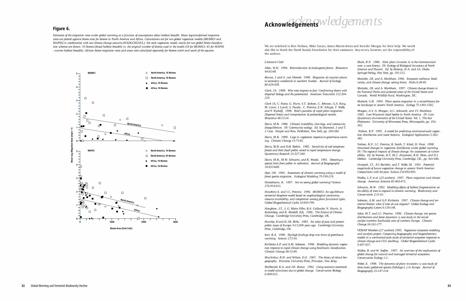
33
Literature Cited
Allen, W.H. 1994. Reintroduction of endangered plants. Bioscience44:65-68.
Brunet, J. and G. von Oheimb. 1998. Migration of vascular plantsto secondary woodlands in southern Sweden. Journal of Ecology86:429-438.
Clark, J.S. 1998. Why trees migrate so fast: Confronting theory withdispersal biology and the paleorecord. American Naturalist 152:204-224.
Clark J.S, C. Fastie, G. Hurtt, S.T. Jackson, C. Johnson, G.A. King,M. Lewis, J. Lynch, S. Pacala , C. Prentice, E.W. Schupp, T. Webb,and P. Wyckoff. 1998. Reid's paradox of rapid plant migration:Dispersal theory and interpretation of paleoecological records.Bioscience 48:13-24.
Davis, M.B. 1986. Climatic instability, time lags, and communitydisequilibrium. IN: Community ecology. Ed. by Diamond, J. and T.J. Case. Harper and Row, Publishers, New York, pp. 269-284.
Davis, M.B. 1989. Lags in vegetation response to greenhouse warm-ing. Climatic Change 15:75-82.
Davis, M.B. and D.B. Botkin. 1985. Sensitivity of cool temperateforests and their fossil pollen record to rapid temperature change.Quaternary Research 23:327-340.
Davis, M.B., M.W. Schwartz, and K. Woods. 1991. Detecting aspecies limit from pollen in sediments. Journal of Biogeography18:653-668.
Dyer, J.M. 1995. Assessment of climatic warming using a model offorest species migration. Ecological Modeling 79:199-219.
Hasselmann, K. 1997. Are we seeing global warming? Science276:914-915.
Haxeltine A. and I.C. Prentice. 1996. BIOME3: An equilibriumterrestrial biosphere model based on ecophysiological constraints,resource availability, and competition among plant functional types.Global Biogeochemical Cycles 10:693-709.
Houghton, J.T., L.G. Meira Filho, B.A. Callander, N. Harris, A.Kattenberg, and K. Maskell, Eds. 1996. The Science of ClimateChange. Cambridge University Press, Cambridge, UK.
Huntley, B and H.J.B. Birks. 1983. An atlas of past and presentpollen maps of Europe: 0-13,000 years ago. Cambridge UniversityPress, Cambridge, UK.
Kerr, R.A. 1996. Sky-high findings drop new hints of greenhousewarming. Science: 273:34.
Kirilenko A.P. and A.M. Solomon. 1998. Modeling dynamic vegeta-tion response to rapid climate change using bioclimatic classification.Climatic Change 38:15-49.
MacArthur, R.H. and Wilson, E.O. 1967. The theory of island bio-geography. Princeton University Press, Princeton, New Jersey.
McDonald, K.A. and J.H. Brown. 1992. Using montane mammalsto model extinctions due to global change. Conservation Biology6:409-415.
Mack, R.N. 1986. Alien plant invasion in to the intermountainwest: a case history. IN: Ecology of Biological Invasions of NorthAmerica and Hawaii. Ed. by Mooney, H.A. and J.A. Drake.Springer-Verlag, New York, pp. 191-212.
Malcolm, J.R. and A. Markham. 1996. Ecosystem resilience, biodi-versity, and climate change: setting limits. Parks 6:38-49.
Malcolm, J.R. and A. Markham. 1997. Climate change threats tothe National Parks and protected areas of the United States andCanada. World Wildlife Fund, Washington, DC.
Matlack, G.R. 1994. Plant species migration in a mixed-history for-est landscape in eastern North America. Ecology 75:1491-1502.
Morgan, A.V, A. Morgan, A.C. Ashworth, and J.V. Matthews.1983. Late Wisconsin fossil beetles in North America. IN: LateQuaternary environments of the United States. Vol. 1. The latePleistocene. University of Minnesota Press, Minneapolis, pp. 354-363.
Neilson, R.P. 1995. A model for predicting continental-scale vegeta-tion distribution and water balance. Ecological Applications 5:362-385.
Neilson, R.P., I.C. Prentice, B. Smith, T. Kittel, D. Viner. 1998.Simulated changes in vegetation distribution under global warming.IN: The regional impacts of climate change: An assessment of vulner-ability. Ed. by Watson, R.T, M.C. Zinyowera, R.H. Moss, and D.J.Dokken. Cambridge University Press, Cambridge, UK., pp. 441-446.
Overpeck, J.T., P.J. Bartlein, and T. Webb, III. 1991. Potentialmagnitude of future vegetation change in eastern North America:Comparisons with the past. Science 254:692-695.
Pitelka, L.F. et al. (23 authors). 1997. Plant migration and climatechange. American Scientist 85:464-473.
Schwartz, M.W. 1992. Modeling effects of habitat fragmentation onthe ability of trees to respond to climatic warming. Biodiversity andConservation 2:51-61.
Solomon, A.M. and A.P. Kirilenko. 1997. Climate change and ter-restrial biomes: what if trees do not migrate? Global Ecology andBiogeography Letters 6:139-148.
Sykes, M.T. and I.C. Prentice. 1996. Climate change, tree speciesdistributions and forest dynamics: a case study in the mixedconifer/northern hardwoods zone of northern Europe. ClimaticChange 34:161-177.
VEMAP Members (27 authors) 1995. Vegetation/ecosystem modelingand analysis project: Comparing biogeography and biogeochemistrymodels in a continental-scale study of terrestrial ecosystem responses toclimate change and CO2 doubling. Global Biogeochemical Cycles9:407-437.
Walker, B. and W. Steffen. 1997. An overview of the implications ofglobal change for natural and managed terrestrial ecosystems.Conservation Ecology 1:2 .
Weber, E. 1998. The dynamics of plant invasions: a case study ofthree exotic goldenrod species (Solidago L.) in Europe. Journal ofBiogeography 25:147-154.
acknowledgementsAcknowledgements
We are indebted to Ron Neilson, Mike Garaci, James Martin-Jones and Jennifer Morgan for their help. We wouldalso like to thank the David Suzuki Foundation for their assistance. Any errors, however, are the responsibility ofthe authors.
32 Global Warming and Terrestrial Biodiversity Decline
Figure 6.Estimates of the migration rates under global warming as a function of assumptions about habitat breadth. Mean log-transformed migrationrates are plotted against biome area for biomes in North America and Africa. Calculations are for two global vegetation models (BIOME3 andMAPSS) in combination with one climate change scenario (HADGCM2SUL). For each vegetation model, results for two global biome classifica-tion schemes are shown: 10 biomes (broad habitat breadth) vs. the original number of biomes used in the model (18 for BIOME3; 45 for MAPSS- narrow habitat breadth). African biome migration rates and areas were calculated separately for biomes north and south of the equator.
5
4
3
2
1
0
5
4
3
2
1
0
BIOME3
MAPSS
Mea
n Lo
g (M
igra
tion
Rat
e (m
/yr)
+1)
0 1000 2000 3000
Africa
North America
Africa
North America
Biome Area (Grid Cells)
•
• • •
•
• •
•
•
•
••
••
••••
•
•
••
•
••
•
•
•••
•
North America, 10 Biomes
North America, 18 Biomes
Africa, 10 Biomes
Africa, 18 Biomes
North America, 10 Biomes
North America, 45 Biomes
Africa, 10 Biomes
Africa, 18 Biomes

34 Global Warming and Terrestrial Biodiversity Decline
1 The climate models (General Circulation Models) included older-gener-ation equilibrium models, newer-generation transient models, andmodels with and without the cooling effects of sulphate aerosols. Thevegetation models (MAPSS and BIOME3) included versions with andwithout direct physiological effects of CO2 (which have been posited toincrease the water use efficiency of plants).
2 If the variables are plotted on logarithmic scales, the increase is close tolinear.
3 The older general circulation models used simple mixed layer oceans tosimulate equilibrium climate under 2 x CO2 forcing and includedmodels from the Goddard Institute for Space Studies (GISS), theGeophysical Fluid Dynamics Laboratory (GFDL-R30), Oregon StateUniversity (OSU), and the U.K. Meteorological Office (UKMO). Thenewer (transient) models included two were from the U.K. HadleyCentre (HADCM2GHG and HADGCM2SUL) and one from the MaxPlanck Institute for Meteorology (MPI-T106). These models made useof coupled atmospheric-ocean dynamics and in one case(HADGCM2SUL) incorporated the cooling effect of atmosphericaerosols (sulfates). The course grids of the GCMs were interpolated to0.5degree latitude/longitude grids. Climate change scenarios were created by applying ratios and differences from 1 x CO2 and 2 x CO2simulations back to a baseline monthly climate dataset (see Neilson etal. 1998). To calculate future climate from the transient GCMs, a 30year (Hadley Centre) or 10 year (Max Planck Institute) climate average was extracted from the current period (e.g., 1961-1990) andthe period approximating 2 x CO2 forcing (e.g. 2070-2099). Neilsonet al. (1998) used a similar set of models to investigate global changesin biome area, leaf area index, and runoff.
4 MAPSS and BIOME3 were run under the two Hadley Centre scenar-ios, whereas only BIOME3 was run under the Max Plank Institutescenario and only MAPSS was run under the GFDL, GISS, OSU,and UKMO scenarios. Global vegetation models that made use of theHadley Centre and MPI climate were run both with and without directCO2 effects, whereas in keeping with the VEMAP analyses, the olderclimate change scenarios were run only with direct CO2 effects (Neilsonet al. 1998). MAPSS and BIOME2 (a precursor to BIOME3) pro-duced generally similar results for the coterminous United States.However, compared to BIOME2, the modelled vegetation in MAPSSwas consistently more sensitive to water stress, producing drier futureoutcomes, and had a larger benefit from the direct physiological effectsof increased CO2, particularly the ability of plants to use water moreefficiently (VEMAP Members 1995).
5 In both distance calculation methods, distances between cell centreswere calculated using software from the United States NationalOceanic and Atmospheric Association (FORTRAN subroutineINVER1, written by L. Pfeifer and modified by J. G. Gergen) using the1984 World Geodetic System reference ellipsoid (WGS84). The shortestpath calculations made use of Dijstra’s algorithm.
6 We classified 0.5-degree cells as “highly” impacted if 55 or 85% of theunderlying 1-km-resolution cells were human-modified (i.e., theirUSGS land cover type designations contained the words “crop,”“field,” “irrigated,” “town,” or “urban” [16 of the 94 USGS landcover types]).
7 These comparisons of biome breadths were undertaken for one climatechange scenario only (HADGCM2SUL). Biomes with fewer than 20grid cells were excluded from the plots.
8 Average migration rates were significantly lower for BIOME3 than forMAPSS. Respective log-transformed means (log10[migration rate +1])were 0.93 (sd = 0.10, n = 6) and 1.26 (sd = 0.18, n = 8); ANOVAF1,12 = 16.07, p = 0.002. BIOME3 consistently had more cells withlow migration rates (<316 m/yr) than MAPSS, comprising on average71% vs. 61% of cells, respectively (see Figure 2). Conversely,BIOME3 had consistently fewer cells than MAPSS in the 316-1,000m/yr class, and although not always consistent among the climatemodels, fewer in the 1,000-10,000 m/yr class.
9 Among MAPSS runs, older climate models had significantly higherlog-transformed migration rates than newer models. Respective log-transformed means were 1.38 [sd = 0.18, n = 4] and 1.14 [sd =0.06, n = 4]; F1,6 = 5.99, p = 0.05.
10 A two-way ANOVA comparing Hadley Centre results according to thevegetation model and whether or not sulphate cooling was used indi-cated not only that BIOME3 had lower rates on average than MAPSS,but that models with sulphate cooling had slightly lower averagemigration rates than the models without cooling. Respective means oflog-transformed rates were 0.95 [sd = 0.20, n = 2] and 1.08 [sd =0.18, n = 2]; ANOVA F1,1 = 58.05, p = 0.08.
11 For BIOME3, incorporation of increased water use efficiency throughdirect CO2 effects led to consistently and significantly lower log-trans-formed migration rates, however the same was not true for MAPSS.For BIOME3, paired-t = -8.41, p = 0.02, mean difference betweenpair-specific averages was 0.15, n=3. For MAPSS, paired-t = 0.57, p= 0.66, mean difference between pair averages was 0.01, n=2.
12 After transforming back to nonlogged values, y-intercepts of linearregressions were 109 m/yr for North America and 30 m/yr for Africafor MAPSS and, respectively, 53 and 5 m/yr for BIOME3.
end notesEnd Notes
WWF Climate Change Campaign
Global warming and climate change pose a serious threat to the survival of manyspecies of plants and animals and the well-being of people around the world. By 2001,WWF aims to ensure that industrialized nations set in motion a permanent downwardtrend in their domestic emissions of carbon dioxide-the leading global warming gas-asthe first step towards substantial reductions by 2010.
WWF Climate Change CampaignDirectorJennifer Morganc/o WWF US1250 24th Street, NWWashington, DC 200037USA
Tel: +1 202 822 3455Fax: +1 202 331 2391E-mail: [email protected]: www.panda.org/climate
© 1986,W
WF ®
WW
F Registered Trademark O
wner