Electronic copy available at: http://ssrn.com/abstract=1480463

Globalization and Asset Prices

Geert Bekaert

Xiaozheng Wang

Columbia Business School

October, 2009

Abstract

We investigate whether the globalization process of the last thirty years has lead to

“convergence” of asset prices in a wide set of countries, encompassing both developed

and emerging markets. We examine several measures of convergence for interest rates

(real and nominal) and bond and equity returns, and important fundamentals as inflation

and earnings growth rates. While doing so, we extensively review the extant literature.

Our results do not indicate strong effects of globalization on the convergence of asset

prices, even though we document some links. In particular, financial openness matters

relatively more than measures of corporate governance and political risk.

Electronic copy available at: http://ssrn.com/abstract=1480463

1

1 Introduction

Much ink has flowed discussing the effects of globalization on financial markets and the

real economy. The literature is so voluminous that providing a comprehensive survey is

nearly impossible. Fortunately, a number of summary articles already exist. Bekaert and

Harvey (2003) survey both the real and financial effects of financial openness, mostly

focusing on equity markets. The evidence on the real side remains controversial. The

survey articles by Eichengreen (2001) and Kose, Prasad, Rogoff and Wei (2009)

conclude that the empirical evidence on the benefits and costs of capital account

liberalizations remains mixed, whereas Henry (2007)’s reading of the literature sides with

Bekaert and Harvey’s (2003) view that capital account liberalization has promoted

growth. Studies that actually take the dynamics of liberalization seriously such as

Bekaert, Harvey and Lundblad (2005), Quinn and Toyoda (2008) and Gupta and Yuan

(2008), do find robust positive growth effects. The evidence in terms of the effect of

financial openness on real volatility and a country’s vulnerability to crises remains mixed

(see Bekaert, Harvey and Lundblad (2006), Kose, Prasad and Terrones (2006)). A

consensus is growing that the relationship between financial openness and economic

growth and volatility is subject to “threshold effects”, with countries with better

macroeconomic policies and institutions (including better developed financial sectors)

responding better.

One important channel through which financial globalization affects the real

sector is through its effects on asset prices. Stulz (1999) concludes that opening a

country to portfolio flows decreases its cost of capital without adverse effects on its

security markets while Karolyi and Stulz (2003) argue that despite globalization, standard

international asset pricing theory fails in explaining the portfolio holdings of investors,

equity flows, and the time-varying properties of correlations across countries. Both

survey articles and Bekaert and Harvey (2003) primarily focus on equity markets, as does

the bulk of the academic literature.

In this article, we characterize the link between the globalization process and the

comovement of asset prices. To do so, we start by providing a simple quantitative

definition of “globalization,” distinguishing between economic and financial

globalization and between de jure and de facto integration. Folklore wisdom suggests

Electronic copy available at: http://ssrn.com/abstract=1480463

2

that integration should lead to “convergence” of asset prices and returns across countries.

Using a large panel of data, we examine several measures of convergence and their link

to quantitative measures of globalization. We investigate bond and equity returns and

several of their components (like real rates, cash flow growth rates etc.). Consequently,

our survey casts a wider net than the existing literature in terms of assets considered,

extending the evidence beyond equity markets. We also use several different measures of

globalization, contrasting, for example, the effects of trade and equity openness. Our

comprehensive examination may shed light on why many studies fail to document strong

evidence of convergence in returns (see the discussion in Pukthuanthong and Roll

(2009)).

The survey article by Stulz (1999) and much of the literature focuses on first

moments. We do not provide further evidence regarding the important question whether

globalization has reduced the cost of capital in the countries opening up to global capital

markets, and we do not provide a comprehensive survey of this literature. For emerging

markets, several studies (Bekaert and Harvey (2000), Henry (2000), Kim and Singal

(2000)) find that stock market liberalization decreases the cost of capital, although the

estimated magnitudes differ. Evidence from American Depositary (ADR)

announcements corroborates these findings (see, for example, Foerster and Karolyi

(1999)). These studies avail themselves of several broad liberalization programs

introduced in many emerging markets at particular points in time. However,

documenting the cost of capital effects of the globalization process in general, especially

in developed countries, which are gradually integrating in world capital markets, is

considerably more difficult. Some limited evidence suggests that the cost of capital

decreases when there is an increase in the degree of globalization (see, for example,

Hardouvelis, Malliaropoulos and Priestley (2004), De Jong and De Roon (2005)).

We generally find weak evidence of asset price convergence linked to

globalization. The evidence is somewhat stronger for interest rates and bond returns than

for equity returns. Focusing on risk premiums also yields stronger results. Strong

cyclical variation in comovement measures weakens the power of most convergence

tests. More powerful evidence in favor of an openness effect results from linking global

3

betas to openness measures. Within such a framework, we show that financial openness

affected convergence more than do measures of corporate governance and political risk.

The remainder of the article is organized as follows. The second section defines

and discusses our globalization measures. The third section summarizes the asset return

data we examine and reflects on where we should expect convergence and where not.

The fourth section explains our general methodology. We investigate 4 different

measures of convergence, and discuss the results of each in turn from Sections 5 to 8.

The final section summarizes our main results and considers several additional empirical

analyses to help interpret them.

2 Defining globalization

We are interested in two aspects of globalization: economic integration, brought about by

trade links, and financial integration, brought about by free capital flows. Measuring

integration is fraught with difficulty and the topic of a large literature in itself. In

particular, de jure openness may not mean that markets are fully integrated because other

factors, such as political risk and poor liquidity, may cause segmentation (see Bekaert

(1995) and Bekaert, Harvey, Lundblad and Siegel (2009) for related analyses);

conversely investment barriers may not prevent actual capital flows. Aizenman and Noy

(2000) also show that there are important links between trade openness and financial

openness, arguing that capital controls in trade-open countries are likely ineffectual. Our

primary interest is “de jure” measures of globalization. This focus is important because

ultimately whether the trend towards globalization continues or not is mostly in the hands

of policy makers. Also, Bekaert, Harvey and Lumsdaine (2002) identify endogenous

dates of market integration from economic and financial data, finding them to be mostly

later than dates of market reform, suggesting that de jure financial openness does lead to

effective integration, albeit with a lag.

For trade openness, Wacziarg and Welch (2008) built an extensive cross-country

data set building on Sachs and Warner’s (1995) classification of countries in either open

or closed countries based on 5 criteria. These criteria involve the magnitude of tariffs,

nontariff barriers, state control of the trade sector, etc. Being a 0/1 dummy, the measure

displays very little cross-sectional variation towards the end of the sample, and actually

4

may not fully reflect the still ongoing trend towards more openness and it cannot capture

the reversal in trade openness observed since the start of the 2008-2009 financial crisis.

We therefore work instead with a more de facto measure: exports + imports divided by

GDP of the current calendar year, denoted by TOi,t.

There are in fact substantially more data available on de jure financial

globalization. We use a measure that combines information from four sources (with each

weighted 1/4), but is skewed towards equity liberalization. The first component is the

measure of capital account openness, compiled by Quinn and Toyoda (2008), and based

on IMF data. They assess the degree of capital account openness based, inter alia, on the

presence of taxes on foreign investment, leading to an index between 0 and 4. We take

the data from Bekaert, Harvey and Lundblad (2005), which map the index onto the [0,1]

domain. The second component is the official liberalization dummy created by Bekaert

and Harvey (2002). The dummy is zero until a country opens its equity market to foreign

investment. This measure does not take into account the potentially binding foreign

ownership restrictions used by many countries, such as Korea, early on in their

liberalization programs. We therefore also use a measure that tracks the market

capitalization available to foreigners as a fraction of total market capitalization (see

Bekaert (1995), Edison and Warnock (2003)). Finally, we use an adjusted version of the

Chinn-Ito (2008) measure of openness. Their measure essentially represents the first

principle component of 4 dummy variables on the restrictions on external accounts drawn

from the IMF’s Annual Report on Exchange Arrangements and Exchange Restrictions

(AREAER). We map the measure onto a [0,1] scale by subtracting the minimum value

of the index over the sample (all countries, all data points) and dividing by the difference

between maximum and minimum. We indicate the aggregated measure of the four

components by FOi,t.

Our final measure of openness focuses on Foreign Direct Investment. FDI can be

viewed as a long-term persistent portfolio flow, but increased FDI also tends to increase

the real links between countries through trade and technological transfers. We use IOi,t to

denote the sum of FDI Assets and FDI Liabilities divided by the GDP of the current

calendar year. All data sources and variable definitions are further detailed in the data

appendix Table A-1.

5

Our sample consists of 34 countries, with varying sample sizes. We therefore

look at 5 different country groups, which are listed in Table 1. For developed countries

we have the longest data sample, and we use data from 1980:1 to 2008:12 for 14

countries. We also consider a subset of 6 EU countries. For a shorter sample starting in

1990, we can also look at 11 emerging countries. We look at them separately and

together with a set of developed countries. For this sample, we can also investigate a

wider set of 14 EU countries. These sample choices are entirely driven by data

availability and the desire to create samples that are as balanced as possible1. We wanted

data not only on openness, but also on equity and bond returns, interest rates, inflation,

etc.

Figure 1 graphs the openness measures averaged over our set of countries over

time. The openness level is generally higher in developed than in emerging markets.

The capital market openness measures clearly show an overall upward trend, but the trade

openness measure, for developed countries, declines before 1990, then again trends

upward. Note that because the trade openness measure involves monthly imports and

exports, it is much more volatile than the other two measures. We therefore show the 1-

year sum of the original numbers in the graph2. Towards the very end of our sample, the

global recession reduces international trade activity and appears to have reversed the

trend towards trade openness. For developed countries, financial openness is almost

complete by the beginning of our sample, but still continues during the 1985-1990 period,

when countries such as New Zealand, Japan, France, Italy and Belgium further

liberalized their capital markets. For emerging markets, a wave of liberalizations

occurred in the early 1990s. The FDI openness measures have also increased

substantially over time; with, perhaps surprisingly, the rate of increase faster for

developed markets than for emerging markets. Conducting trend tests for the various

1 Appendix Table A-2 contains the various sample periods available per variable and per country, showing

the remaining sources of unbalanced samples (e.g. Austria’s nominal short rate becomes only available in

1987). 2 While the other openness measures are graphed in their original form, in the empirical work below, we

often construct moving averages of the openness measures matching the window frames for the

convergence measures.

6

measures, all the openness variables feature a positive trend coefficient, except the TO

measure for the 2 long samples. However, the trends are not statistically significantly

different from zero.

Table 2 reports summary statistics for the openness measures (Panel A) and their

correlations (Panel B). In most cases, the measures are highly positively correlated, with

correlations mostly exceeding 0.8. One exception is the correlation between TO and FO

in the long sample, which is negative due to the downward trend of trade openness in the

mid 1980s. This trend also reduces the correlation with IO for these samples.

We do not use a popular alternative measure of openness, due to Lane and Milesi-

Ferreti (1999), which records the ratio of foreign assets and foreign liabilities over GDP.

Their gross measure adds up the stocks of direct investment, portfolio equity, debt assets

(liabilities) and foreign exchange reserves, thereby covering all securities in IMF’s

International Investment Position, and divides the aggregate number by annual GDP.

However, the measure is very highly correlated with both FO and especially IO. The

correlation with the latter, computed as in Table 2, always exceeds 99%. It therefore

makes little sense to include the measure in addition to the ones we already analyze.

3 Asset prices

Theory

Generally, we are interested in tracing out the effects of globalization on returns to the

two main asset classes, equities and bonds, and their components. Figure 2 provides an

overview. To price equities, we need (expected) cash flows and discount rates. The

discount rate for stocks can be split up in three components: a (short-term) real rate, a

term premium, and an equity premium. For nominal bonds, we only need to consider

discount rates, the real rate and the term premium, but we also investigate inflation as it is

the most important variable driving time-variation in nominal bond yields (see Ang,

Bekaert and Wei (2008) and many others).

How will globalization affect the comovement of these various variables across

countries? Let’s start with real interest rates. Under real interest rate parity, real interest

rates are equalized across countries. However, real interest rate parity requires the strong

and somewhat unpalatable assumptions of uncovered interest rate parity, purchasing

7

power parity and the Fisher hypothesis in both countries to hold. That is, full money

market integration does not suffice, as it does not preclude the existence of currency and

country risk premiums. Nevertheless, one would expect globalization to contribute to

real rate convergence across the world, as open financial markets help equalize real

returns to capital invested. While financial market integration should be the major force

affecting interest rates, under imperfect integration, trade openness may have important

effects. Imagine a closed-economy world, in which real rates reflect expected real

growth rates and local precautionary savings motives. Theoretically, the effect of trade

openness is not clear. Trade integration may lead to specialization, which should lower

output correlations across countries and thus likely imply real rate divergence, but it may

also lead to synchronization of business cycles through demand spillover effects.

The effect of openness on business cycle convergence has been studied

extensively in the literature, but mostly the focus is on financial openness. In fact, most

theoretical models predict that financial market integration leads to business cycle

divergence, either through specialization towards the higher return projects as in Obstfeld

(1994); or the attraction of capital to positive productivity shocks as in Baxter and

Crucini (1995). The empirical evidence is decidedly mixed (compare Kalemli-Ozcan,

Papaioannou, and Peydro (2009), who find divergence, with Imbs (2004), who finds

convergence). However, unless capital market distortions exist, interest rates may still

equalize under full market integration. Comparing short versus long term real interest

rates, monetary policy should exert more of an influence on short term interest rates,

making convergence more likely to be observed for longer term interest rates. Of course,

this is no longer true if there is abundant monetary policy coordination, or if in the limit,

as happened in Europe, countries join monetary unions.

A simple perspective on the convergence of nominal interest rates is a Fisherian

world, where nominal interest rates equal real interest rates plus inflation expectations

(and perhaps inflation risk premiums). We discuss inflation below. An international

perspective is the uncovered interest rate parity condition, where nominal interest rates in

one country equal the interest rate in another country plus expected exchange rate

depreciation. These exchange rate expectations may then be linked to inflation

expectations through purchasing power parity. The relationship may not hold because of

8

the presence of currency risk and country risk premiums. Importantly, open financial

markets and free trade need not lead to equalization of interest rates (see also Frankel

(1989)), but it should lead to the disappearance of certain country premiums, caused by

capital controls. The creation of a monetary union, as happened in the context of the

European Union in 1999, obviously must lead to a convergence of nominal interest rates,

and it mostly did so within Europe (see Baele et. al. (2004), Jappelli and Pagano (2008)).

One may still observe some divergence for long term bond yields, however, simply

because of the presence of liquidity premiums in various bond markets.

Generally, inflation is of course an important state variable driving bond returns

(although it may also affect equity returns). Globalization may affect the inflation

process through a variety of channels. Trade openness generally increases the level of

competition in both product and labor markets. Openness means increased tradability

and substitutability of products and services across countries; increased contestability of

both output and input markets and increased availability of low-cost production in

previous command economies, such as China, etc. Rogoff (2003) and Lane (1997) argue

that globalization decreases the central bank’s incentive to inflate. Chen, Imbs and Scott

(2009) and Cox (2007) stress how globalization raises productivity growth, and therefore

inflation. On balance, these effects may contribute to inflation convergence across

countries (see Chen, Imbs and Scott (2009)). For example, one interesting recent

hypothesis is that international trade has made it possible for many countries to import

low inflation from China, and withstand the rather strong inflationary forces coming from

the recent commodity price shocks. Globalization should make country-specific inflation

more sensitive to global excess demand conditions, although this of course also depends

on exchange rate movements. Borio and Filardo (2007) show that, especially since the

early 1990s, the role of global economic slack in explaining domestic inflation has

substantially increased.

Globalization, together with improved central bank institutions and practice, may

also have played an important role in the global trend towards lower inflation, witnessed

over the last 20 years (see Rogoff (2003)). It is also conceivable that the real shocks

buffeting the world economy were simply milder over the last few decades, and that the

current crisis will eventually usher in another era of higher inflation. With its lower

9

level, we have also witnessed a decrease in inflation volatility (part of the so-called

“Great Moderation” phenomenon). Table 3 shows the average of the country-specific

means and annual volatilities of inflation during three sub-samples: 1980s, 1990s and

2000s. First note that emerging markets have higher inflation and inflation variability

than the developed group in all the sub-samples. More importantly, inflation and its

variability decrease substantially over time in both groups.

There is in fact a big debate raging in macroeconomics about the causes of the

“break” in volatility, which has not settled yet at a time where it is becoming painfully

obvious this “Great Moderation” has come to an end. For our purposes, these trends are

nonetheless important. The lower level and variability of inflation may affect

comovement measures. At first glance, a substantially lower level of inflation may lead

to convergence; the decreased variability at the world level, on the other hand, may lead

to decreased comovement (see Section 2.6), if it is caused by the lower variability of

global inflation shocks.

An important part of the variation in bond returns and, even more so, in equity

returns comes from variation in risk premiums. Here, we expect financial market

integration to be the main driver behind the convergence of term- and equity premiums

across countries. In integrated economies, securities of similar risk should command the

same risk premiums and we should likely observe risk premiums converge.

Finally, how should globalization affect the correlation of cash flows across

countries? Here the debate on the effects of openness on business cycle convergence is

relevant again. Assume for one moment that cash flows are positively correlated with

output. Then, the theoretical literature would suggest that financial market integration

may lead to business cycle divergence and hence to lower cash flow correlations, through

the effects discussed earlier. Recall that trade openness has ambiguous effects on output

growth correlations. Now, of course, how output translates into cash flows is an entirely

different matter, which may depend on the competitive structure in particular countries.

Ammer and Mei (1996), for example, find that cash flow growth rates are more highly

correlated across countries than are output growth rates.

10

Measurement

We would like to split up returns into its main drivers (discount rates, split up over term

structure effects and risk premiums, and cash flows), but we want to minimize relying on

parametric assumptions in this article, and preferably only use variables we can measure

from the data directly.

In the middle of Figure 2, we show real rates and term premiums as major

components of the discount rate for both equities and bonds. The real rate plus the real

term premium (the difference between the long and short rate), is the real long rate. The

remainder of the discount rate is a risk premium. Measuring ex-ante real rates is

impossible without a model for expected inflation and inflation risk premiums. We make

the simplest possible assumption for expected inflation, namely that the best forecast of

future inflation is current (annual) inflation. While we do not believe that inflation is a

random walk process in all of our countries, there is some evidence that random walk

inflation forecasts are hard to beat for the US (see Atkeson and Ohanian (2001), and Ang,

Bekaert and Wei (2007)). Finding more sophisticated inflation forecasts for all of these

countries is next to impossible. Our short rates are very short-term, mostly reflecting a

three-month maturity; therefore we can safely assume a zero inflation risk premium3.

Hence, we compute the real short term rate as the difference between the nominal short

rate and (current) inflation.

For long term rates, let’s consider the following decomposition of the long-term

nominal rate, in,t:

i , r , π , φ , (1)

where rn,t is the real long rate (ex-ante), , is the average expected inflation over the life

of the bond and φn,t is the long-term inflation risk premium.

If inflation is a random walk, the best forecast for inflation over a longer time

period is also current inflation. We therefore compute the long-term real rate also as the

difference between the long-term nominal rate and current inflation, but here we are on

considerably shakier ground. Even for developed countries, most studies seem to agree

that inflation risk premiums can be sizable and vary through time (see Bekaert (2009) for

3 We use continuously compounded rates, expressed in per annum terms.

11

a survey) 4 . Under these strong random walk and zero inflation risk premium

assumptions, the real term premium equals the nominal term premium.

For completeness, we also look at nominal short and long rates and at inflation

itself.

Of course, we also investigate the returns themselves, and consider three versions

for both equities and bonds: the actual return, the excess return (defined as the return in

excess of the nominal short rate), both expressed in dollars, and a hedged excess return.

We approximate the latter by investigating local currency excess returns. In addition, we

consider a number of equity-related variables. We examine cash flow growth, measured

as the year-on-year earnings growth rate: ln / where

and EAt = MCAPt/PEt measured in U.S. dollars. Because there is mostly

quarterly reporting on earnings, we first aggregate the reported earnings in the recent 3

months to smooth the series. Using annual growth rates is necessary to control for the

strong seasonal patterns in earnings.

We also investigate a valuation ratio, namely the log of the price earnings ratio

(PE, henceforth). Valuation ratios reflect both discount rates and growth opportunities,

but at least they are real concepts and should not have a currency component.

Table 4 provides summary statistics for the variables of interest in this paper. For

each variable, we first compute the time-series mean of the variable for each country,

then obtain the cross-sectional mean and standard deviation across either developed

countries or emerging markets. Comparing developed and emerging markets, developed

markets on average have relatively lower interest rates, and higher returns, higher PE

ratios and lower cash flow growth. Standard deviations of these variables are uniformly

higher in emerging markets.

4 One potential procedure to correct for time-varying inflation risk would compute rolling inflation

volatility for all of our countries, and then run a panel regression of our current real rates for each country

on inflation volatility, with potentially the coefficient depending on emerging versus developed countries.

We could then take the current long term real rate minus the pooled regression coefficient times current

inflation volatility as the estimate of the true ex-ante real long term rate.

12

4 Methodology

We seek to answer two simple questions. First, do we observe a pattern of cross-country

convergence in returns and their components over time? Second, is this pattern related to

openness? We do not take a strong stance on a measure of convergence. Instead, we

examine four different measures, each with pros and cons: correlations, global betas,

panel country-effect standard deviations and cross-sectional dispersion. We discuss these

measures in more detail in separate sections devoted to each.

To detect quasi-permanent movements in convergence/divergence measures, we

use trend tests. This may appear strange at first, as it is quite possible that some measures

may move to a point where they can no longer converge further. Also, if de jure

liberalizations drive changes in the measures, a break analysis around the liberalization

dates would appear superior. However, recall that we are interested in the convergence

of variables across countries. Consequently, they are affected by liberalizations in all the

countries in the sample. Given sufficient cross-sectional and temporal variation in the

liberalizations over time, the pattern should look like a slow trend over time, as the

globalization process itself, see Figure 1. This is true even if the “break” in one country

is sudden and abrupt. Even so, in many countries or regional groups (such as the EU),

integration itself has been rather gradual. For instance, Korea relaxed foreign ownership

restrictions starting in 1991, in slow increments, to finally become totally open in 2002.

The benchmark model for the trend test is

yτ = α0 + α1 τ + uτ (2)

where yτ is the variable of interest, and τ is a linear time trend. We use the test developed

by Bunzel and Vogelsang (2005), which is robust to I(0) and I(1) error terms and uses a

“Daniell kernel” to nonparametrically estimate the error variance needed in the test. Our

relatively small sample necessitates the use of a powerful test, and the Bunzel-Vogelsang

test has optimal power properties.

In addition, we also directly investigate the link between convergence of various

economic variables and our openness variables. To this end, we specify multivariate

regressions of the form:

CONVt = α + β1 TOt + β2 FOt + β3 IOt + γ Zt + εt (3)

13

where CONVt is the convergence measure and Zt are control variables we discuss below.

Because the error terms are likely serially correlated, we use a Cochrane-Orcutt

estimation method, specifying εt = ρ εt-1 + ut and ut ~ IID. We often also check whether a

trend variable survives in such a specification.

Because we have a relatively small sample in the time series dimension and a

large set of countries to collect data for, it is impossible to allow for a comprehensive set

of control variables Zt. We use two variables that may ex ante have a significant effect

on convergence measures, but may not be directly related to openness. The first is a

global business cycle variable, denoted by Cyct. To measure the stance of the business

cycle, we subtract a moving average of world GDP growth (over the last 5 years) from

current GDP growth. However, we only have end-of-year annual GDP growth. To turn

this into a monthly variable, Cyct is constructed using the weighted average of the annual

world business cycle variable Cycs,a in the current year and last year. For example, in the

mth month of year s, Cyct = ((12-m)/12) Cycs-1,a + (m/12) Cycs,a. It is well known that in

recessions all asset prices are more variable. If a global factor model has some

explanatory power for asset returns, then recessions should lead to financial variables

being more correlated across countries because the global factors are more variable (see

Boyer, Gibson and Loretan (1999) and Bekaert, Hodrick and Zhang (2009)). We actually

find that the global business cycle variable is mildly positively correlated with the

openness variables; suggesting we have had slightly fewer incidences of recessions in the

later part of the sample, which would spuriously lower comovements.

The second variable is a crisis measure, denoted as Crisist. When a significant

number of countries experience a crisis, this may lead to extreme movements in asset

prices. If isolated to a few countries or one region, this could actually decrease the

comovement across asset prices. However, if the crises are global in nature,

comovements may increase. We use the dummies for banking and currency crises

collected by Caprio and Klingebiel (2003) for each country and update the data using the

information in Reinhart and Rogoff (2008). We investigated both equally weighted and

value weighted (using GDP) averages over time. These two crisis variables show no

consistent correlation pattern with the openness measures, being sometimes negatively,

sometimes positively correlated, depending on the country group and the period.

14

The effects of globalization on asset prices have been examined before in a

variety of articles, but most articles have focused on one asset price (with equities being

the most popular), a particular comovement measure or a particular set of countries. We

discuss the extant literature as we go along, but mention a few articles already. Perhaps

the most comprehensive literature has used the stock market openings of emerging

markets at the end of the eighties and the beginning of the nineties to trace the effects of

(a shock to) integration on asset prices, typically using event study-type methodologies.

Bekaert and Harvey (2000), Bekaert, Harvey and Lumsdaine (2002), and Kim and Singal

(2000) investigate many characteristics of equity market data, including correlations with

world market returns. They find that liberalizations increase the correlation with world

market returns. Henry (2000) is more typical of the literature focusing primarily on the

cost of equity capital, finding, as Bekaert and Harvey (2000) do, that openings decrease

the cost of capital. There has also been work on real interest rates, from a variety of

perspectives, but mostly focused on developed markets. Jorion (1996) tests real interest

parity for the US, Britain and Germany, rejecting the hypothesis for all three. Goldberg,

Lothian and Okunev (2003) examine real interest rate differentials for 15 country pairs,

finding no significant differences and a narrowing of differentials over time. Gagnon and

Unferth (1995), looking at 9 countries, estimate a world interest rate, and show that each

country’s real rate is very highly correlated with the world interest rate. Breedon, Henry

and Williams (1999) investigate long run real rates, including rates from inflation-linked

bonds in 7 countries, but fail to find evidence that interest rates are converging towards a

single world rate. Phylaktis (1997) investigates comovements of real rates in the Pacific-

Basin region. None of these real interest rate studies takes the dynamic perspective of

this article linking changes in comovements to changes in actual financial openness.

5 Correlations

The most obvious convergence statistic to investigate is of course the correlation. There

is a long tradition in finance of examining the links between globalization and return

correlations (see for instance, Longin and Solnik (1995), Bekaert and Harvey (2000),

Bekaert, Hodrick and Zhang (2009)). Longin and Solnik (1995) detect an upward trend

in correlations across the G7 countries, but Bekaert, Hodrick and Zhang (2009) only find

15

a significant trend within Europe. Rather than focusing on correlations per se, we

investigate a variance ratio of the form (see Ferreira and Gama (2005)):

∑ ,

∑ ,

for 35, , for any variable x at time t. (4)

This statistic has the sum of the variances in both the denominator and numerator

as a leading term, but then depends on the cross-product of the standard deviations

multiplied with correlations in the numerator and multiplied with 1 in the denominator.

Hence, if the correlations were literally one, the log-ratio would be zero; and the lower

the correlations the more negative is the ratio. By computing the statistic over rolling

three-year intervals, we trace the evolution of correlations over time. Increased

correlations lead to increasing ratios. Note that PRt is a more “efficient” statistic than the

average correlation. For N countries, the latter requires the computation of N×(N-1)/2

correlations, whereas the PR-statistic only requires the estimation of N+1 variances.

Tables 5 and 6 contain the results. Table 5 focuses on the trend test. We do not

find a single significant trend coefficient. This is easy to understand once we glance at

Figure 3, which graphs the (exponentiated) ratios for all the variables. Ratios close to 1

mean perfect correlation. The graphs show that these ratios primarily show cyclical

movements. For the interest rate variables in Panel A, the one variable that seems to

display a bit of a trend is the term premium, the one variable in our set that is closest to a

risk premium. Yet, at the end of the sample, correlations seem to have moved down

again. The large discrepancy between the observations from developed countries and for

the EU long sample in the nominal rates graph during 1987-1980 is primarily driven by

New Zealand, where two recessions during 1985-1991 implied volatile rates. Panel B

shows bond and equity returns. The end of the sample shows closely aligned equity

returns, but comovements for bond returns decrease. It is possible that this is an artifact

of the recent crisis. Cash flow growth and valuation ratios, shown in Panel C, likewise

do not show strong trends, but mostly cyclical behavior.

Table 6 shows the results of our main regression. It is conceivable that there is

still a link with openness once the cyclical movements are controlled for. For example,

the high comovements observed in the beginning of the sample for both short and long

rates in Panel A of Figure 3 coincide with the major recession many developed countries

16

witnessed in the early eighties. If openness increases comovements, we should see

positive and significant coefficients. Unfortunately, there is no clear and consistent

pattern, neither across different samples, nor across variables (even within a group). The

closest we come to this is perhaps with long real rates, where financial and trade

openness always have positive coefficients, which are significant at some level in 4 of the

5 country groups we consider. While the comovement of inflation across countries does

not seem to have been systematically affected by the openness variables, financial

openness continues to have a rather consistent positive effect on nominal rate

comovements as well. For returns, there are a number of significant coefficients, but

absolutely no consistent patterns in terms of signs. If anything, bond return

comovements appear negatively correlated with financial openness. The same lack of

consistency plagues the results for cash flow growth and PE ratios.

Note that in Table 5 superscripts indicate whether a trend term has a significant

positive coefficient in our main regression. This does happen in a few cases, but there is

no clear interpretable pattern.

6 Beta models

The results using correlation as a comovement measure were perhaps a bit disappointing.

However, this is not surprising, because correlations have well-known limitations,

especially when one is looking for rather low-frequency changes in comovement. The

reason is that correlations vary considerably over time, in particular, in response to

movements in the volatilities of underlying factors. Consider a simple one factor model

for a variable xi,t for country i:

xi,t = βi ft + ei,t (5)

Imagine that ft is the “world factor”. An example of such a model would be the

World CAPM, where xi,t would be the country’s equity (excess) market return and ft the

world (excess) market return. It is easy to show that in such a model the correlation

between xi,t and ft equals

, (6)

17

where σi is the volatility of the variable xi,t and σf the volatility of the factor.

Consequently, everything else equal, if the volatility of the factor increases, it increases

the correlation between xi,t and the global factor, and, given that the ei,t’s are

idiosyncratic, increases the correlations among all country variables correlated with f,

provided they have positive betas5. It is well known that the volatility of well-diversified

equity portfolios varies substantially over time without showing significant permanent

changes. Macro variables show distinct cyclical variation in volatility, being higher in

recessions (see Bekaert and Liu (2004), for consumption growth, for example).

Consequently, there is much scope for correlations to show substantial temporary

movements that make it hard to detect the possible underlying trends caused by the

globalization process. In particular, they may temporarily increase when factor

volatilities are temporarily high, a phenomenon we call the volatility bias.

The volatility bias for equity markets is worse in bear markets. Longin and

Solnik (1995) and Ang and Bekaert (2002) show that stock markets are unusually highly

correlated in bear markets, even beyond what can be attributed to the higher variance of

market factors in such market conditions. Consequently, the incidence of bear markets

may play a role in measuring changes in correlations. The controls for global recessions

and crises should mitigate these biases, but they may not suffice.

Looking at equation (5), financial market and trade integration is most likely to

show up in the betas itself. As markets integrate, presumably the dependence on world

factors will increase. The literature here is rather voluminous. Articles that have

parameterized betas as a function of integration indicators (most frequently measures of

trade integration) include Bekaert and Harvey (1997), Chen and Zhang (1997), Fratzscher

(2002), Bekaert, Harvey and Ng (2005), Ng (2000) and Baele and Inghelbrecht (2009).

Note that one has to be careful with such an argument, because if the global factor

simply aggregates the country-specific variables (which would be the case in a strict

application of the World CAPM), the betas have to add up to one, and hence, they cannot

increase for all countries. However, the bulk of the articles we mentioned apply variants

5 See Forbes and Rigobon (2002), Boyer, Gibson and Loretan (1999), Bekaert, Harvey and Ng (2005) and

Bekaert, Hodrick and Zhang (2009) for related discussions.

18

of equation (5) in such a way that these constraints do not apply, for example, by using

the U.S. as the global benchmark.

In this article, we estimate two types of beta models. The first model simply

allows for time-varying betas using a three-year rolling window and computes rolling

variance ratio statistics. The model can be represented as:

xi,t = αi + βi xglob,t + εi,t (7)

where xi,t denotes any variable of interest in country i at time t. We consider two proxies

for the global factor, either xglob,t = , where , is the real GDP per capita weighted

average xj,t over all countries for all the country i except that for Japan, the U.K. and U.S.,

, is the weighted average of xj,t excluding its own country; or xglob,t is simply xUS,t,

which is the U.S. variable. The regressions are estimated country-by-country using OLS.

As in Bekaert and Harvey (1997), Bekaert, Harvey and Ng (2005) and Baele (2005), we

compute variance ratios, that is,

VR ,, ,

, for s t 35, t (8)

These variance ratios measure how much of the total variation in the variable is

accounted for by the global factor, and are therefore closely related to the R2 in the

regression. Pukthuanthong and Roll (2009) in fact propose using the R2 of a multi-factor

model to measure market integration. Using an APT model with 10 factors to compute

time-varying R2’s, they uncover a marked increase in measured integration for most

countries, which is not revealed by simple correlations among country indices.

By computing the variance ratios over rolling three year-intervals, we can trace

the evolution of the importance of the global factor over time. As a first test, we consider

trend tests for these variance ratios. However, while the trend coefficients are often

positive, we fail to find many significant coefficients. One possible reason is that the

volatility bias mentioned before implies that cyclical behavior dominates the dynamics of

the variance ratios and erodes the power of the trend tests. To check if we still on

average see increases in variance ratios over time, Figure 4 graphs the average variance

ratios of individual countries over the 5 country groups for all the variables. The global

factor is xUS,t. It is again difficult to see persistent increases with the exception of the

short rate and term premium series. The equity return variance ratios also seem to

19

increase over time, despite being quite volatile. The increase is especially noticeable for

emerging markets. At the end of sample, variance ratios do tend to increase more

generally but this may reflect the recent crisis. Replacing xUS,t with xglob,t yields similar

patterns.

Because the time series graphs are very noisy, we present the data in an

alternative fashion. Figures 5 and 6 show the average variance ratios in the first and

second halves of the sample period. We use 1980-1994 as the first half of sample and

1995-2008 as the second half for the country groups with the long sample (Figure 5);

1990-1999 as the first half of sample and 2000-2008 as the second half for the country

groups with the short sample (Figure 6). We depict the average VR for the first half of

the sample on the x- and for the second half of the sample on the y-axis. If the country

dots are mostly above the 45-degree line, VR’s increase in the second half of sample

relative to the first half. The results are now much clearer. In the long sample (eighties

and early nineties versus the last 14 years), variance ratios among the interest rate

variables clearly increase for real and nominal short rates and the term premium. There

are very few exceptions, and the term premium variance ratios increase in all countries.

For long rates and inflation, we do not observe a quasi general increase in variance ratios.

For the return variables, a general increase is apparent for the bond returns, but for equity

returns, the results are decidedly mixed, definitely for unhedged returns. While for cash

flow growth rates and PE ratios, most variance ratios increase, it is far from a general

phenomenon. The results for the short sample in Figure 6 are actually quite similar, with

the exception that the increase in variance ratios is less general in nature for the term

premium and not visible at all for inflation. These results are somewhat in contrast with

Eiling and Gerard (2008), who find that equity variance ratios increase for developed but

not for emerging markets. Their methodology is different, however, in that they use high

frequency data but also rely on certain strong parametric restrictions to derive their

results. The figures using xglob,t instead of xUS,t are similar.

We can also directly examine the time-variation in the global beta. Many studies,

mostly focusing on equity markets, have observed that betas with respect to global factors

increased over time. Baele (2005) and Baele, Ferrando, Hordahl, Krylova, and Monnet

(2004) have documented increases in “shock spillovers” with respect to the global

20

market, and Bekaert and Harvey (2000) actually show directly that stock market

liberalizations increase betas.

Our second model attempts to more directly deal with the volatility bias critique

and focuses on how openness affects the beta with respect to the global factor. We

estimate the following panel factor model:

xi,t = αi + αopen Openi,t + αcyc Cyct + αcri Crisisi,t +

(βi + γopen Openi,t + γcyc Cyct + γcri Crisisi,t) xglob,t + εi,t (9)

where Openi,t is either TOi,t, FOi,t or IOi,t. All the other variables were explained before.

The model is estimated using the Cochrane-Orcutt method.

Note that both the constant term for each country and the country’s beta with

respect to the global factor depend on a country-specific fixed effect, on the global

business cycle variable, the country-specific openness measure, and the country-specific

crisis indicator. The latter coefficients must be constrained to be the same across

countries for identification. The coefficient we are interested in is γopen. We do not focus

on level effects in this article. Note that for this regression, it is impossible to let all

openness variables enter the regression simultaneously. While the correlation between

these variables is imperfect, the interactions with the global factor make regressions with

multiple openness measures ill-behaved.

Table 7 reports the results, with Panel A focusing on the world variable as the

benchmark and Panel B on the US.

We first focus on the long sample. In Panel A, it is difficult to see very strong and

consistent patterns. Over the long sample, financial openness has the most consistent

positive and significant effect on global betas. The main exception is the price earnings

ratios where the beta is negatively linked to its world counterpart. Using the U.S.

variable as the global factor, financial openness receives higher and more significant

coefficients, whereas the PE ratios are only weakly negatively linked to financial

openness. Whereas FDI has weak and inconsistent effects with the world benchmark, the

U.S. beta appears mostly positively associated with FDI, being significant in the majority

of cases. The strongest effects of trade openness are on bond returns, where it has led to

LOWER not higher betas. The results for the short sample are in fact roughly consistent

with coefficient patterns observed for all countries and the full sample. However, for

21

emerging markets, this is so with much less statistical significance. Here, FDI seems to

have a stronger effect on global betas than does financial openness. It is also true, for the

short samples, that the U.S. betas with respect to financial openness and FDI yield the

stronger results. One interesting conclusion of Table 7 is that the results for interest rates

and stocks are quite different. For equity returns and its components (including cash

flows), we find financial openness and FDI to mostly have positive effects on global

betas. However, this is not true for interest rates (especially short rates) and inflation,

where the results are decidedly mixed. Perhaps because the term premium is mostly

positively associated with financial openness, bond returns mostly are too, but not always

(see for instance, the emerging market sample). This suggests that it really may be quite

powerful to try to further decompose equity returns into various components, an issue we

return to in the conclusions.

There are a number of possible interpretations of the sometimes weak results,

which we discuss more thoroughly in Section 9. Let us just mention two that have been

the focus of articles closely related to the ones surveyed in this section. First, regional

integration may be stronger than global market integration. Baele (2005) finds this to be

true in Europe. Second, the model may be inappropriate along a number of dimensions.

In particular, the beta with respect to a global factor could reflect changes in both

economic and financial integration, but also many other factors, such as competitive

forces, industrial structure, etc. A number of articles attempt to impose more structure by

specifying an asset pricing model, linking the second moments to the first moments, and

then examining the degree of integration over time (see Bekaert and Harvey (1995);

Carrieri, Errunza and Hogan (2007)). These articles also show that the evolution towards

more integrated markets is not always a smooth process observed for all countries.

7 Country effect standard deviation

Most of our comovement measures thus far have the disadvantage of requiring a rolling

estimation to trace out the effects of globalization. Here, we use a regression model

estimated over the full sample that separates the data into global and country-specific

components, and then uses the cross-sectional standard deviation of the country effects at

each point of time as the measure of interest. Of course, this measure is inversely

22

correlated with comovement. There are an infinite number of ways to split the data into

country-specific and global components, but we restrict ourselves to the simplest possible

model with fixed effects6:

xi,t = μ + gt + αi + ei,t (10)

Because many of our variables are quite persistent, we again use the Cochran-

Orcutt method, with country-specific autocorrelations, to estimate the model. The

country fixed effects and time effects sum to zero, so we can think of gt+μ as the global

component at each point in time. Gagnon and Unferth (1995) use such a model to

estimate the world interest rate using data from 9 countries. The country-specific

component is of course αi+ei,t, and it is its cross-sectional variation that we are interested

in. We consider two variants:

∑ , and (11)

∑ , (12)

These measures are available at each point in time, and we can consequently

perform a trend analysis and multivariate regressions as we did for the PR measure.

Table 8 reports the results for the trend tests on the CESD measure. Convergence

would be reflected in negative trend coefficients and we find the trend coefficients to be

over-whelmingly negative. Unfortunately, only 7 out of a total of 70 coefficients are

significantly different from zero, of which two for the term premium variables and four

for bonds returns. One problem, especially for the emerging markets sample, is that

crisis periods may cause rather big outliers. For example, the Mexican and South-East

Asian crises cause spikes in interest rates in a few countries and extreme observations for

equity returns as well that affect the measure. We obtain a very similar picture from

CESDALT, so we do not report trend results for that measure.

Table 9 reports the results from regressing the CESD measure on our openness

variables while controlling for global business cycles and crises. The significant

coefficients are mostly concentrated in the long samples (developed and EU markets) and

6 For example, Kose, Otrok and Whiteman (2003) and Kose, Otrok and Prasad (2008) employ Bayesian

dynamic latent factor models, with world, regional and country-specific factors to study global business

cycles.

23

in the interest rate variables. The most robust result appears to be that increased FDI

leads to smaller country effects. Do note that FDI is relatively highly correlated with our

financial openness variable. For nominal interest rates, for example, the positive

coefficient on IO is likely offset by the bigger negative coefficient on the FO variable.

Most of the negative effects we see elsewhere are due to either IO or FO. Nevertheless,

many puzzling results remain; for instance, it is unclear why the country-specific

variation in PE ratios should increase with trade and financial openness for the emerging

market sample.

We also use the panel model to extract the world interest rate process, that is,

gt+μ. Figure 7 first graphs the world interest rate (both the short and long real rates)

extracted from the long developed countries sample, and then graphs the European real

long interest rate, extracted from the European Union countries (we consider both the

long and short sample). The graphs use the country effect standard deviation at each

point in time to graph a “cross-sectional” standard error band around the estimates. The

“world interest rate” climbs above the 4% level in the mid eighties and stays elevated till

the end of 1993. Since then we see a non-smooth decrease in the level of interest rates,

decreasing to almost zero in the current crisis. The cross-sectional standard deviation,

our measure of convergence, decreases largely with the level of interest rates. The long

real rate shows a very similar pattern but stays elevated longer. In the European Union

countries, we observe the same pattern, but the monetary integration process and the

introduction of the euro in 1999 make the cross-sectional standard deviation decrease to

very low levels.

8 Cross-sectional dispersion

The last measure we examine is cross-sectional dispersion:

CSN

∑ x , x ,N where x , N

∑ x ,N (13)

This statistic simply measures how dispersed a variable is around its cross-

sectional mean at each point in time. The statistic has obvious appeal as we would expect

that full market integration could in many instances lead to very low cross-sectional

24

dispersion, and the statistic can be computed at each point in time, without any sample

history.

Table 10 reports the usual trend tests for this measure. As with our previous

convergence measure, the signs are overwhelmingly negative; but statistical significance

is mostly lacking. We now find 11 statistically significant negative trends, again all

concentrated in the interest rate and bond return variables. It is interesting that we find

the strongest evidence of convergence in the asset variables that have received

considerably less attention in the market integration literature, which has mostly focused

on equities. Of course, these findings may simply reflect the limited power of trend tests,

and the fact that interest rates and bond returns are less noisy than equity returns.

In Table 11, we report results of a multivariate regression of the cross-sectional

dispersion of our economic variables on our openness measures. If the trend towards

globalization served to decrease dispersion significantly, we should observe significant

negative coefficients on the openness variables. Focusing first on the long developed

country sample and the interest rate variables, there seems to have been a significant

downward trend in dispersion, mostly associated with increased FDI flows. This is also

true for inflation. Not surprisingly, this also translates into the increase in FDI over time

being associated with less dispersion in bond returns. However, these coefficients are not

significantly different from zero. For equity returns, the coefficients on FDI are negative

but insignificant. For the coefficients on trade and financial openness, we find negative

coefficients for equity returns, but mixed results for bond returns and the interest rate

variables. When we investigate cash flow growth and valuation ratios, we find overall

negative coefficients, with the coefficients being most significant for financial openness.

These patterns are largely preserved for the EU countries, where we observe more

significant coefficients, also associated with financial openness.

Moving to the shorter sample, for emerging markets we also find overall mostly

negative coefficients, but statistical significance is more elusive. Equity return dispersion

is significantly negatively associated with FDI, but the coefficients on trade and capital

market openness are positive, albeit not significant. We now see a few significant

positive coefficients, which are hard to explain. For the all countries and EU short

25

sample, the results look more like the long sample results, but with overall less

significance.

Figure 8 graphs the cross-sectional dispersion measures over time. While some

downward trending behavior is apparent for all variables, the graphs also show cyclical

and extreme behavior, which is mostly driven by crises. For example, the spikes in 1996

for the interest rate variables are mainly driven by Mexico’s high interest rates during the

Mexican financial crisis. The spikes in nominal and real rates, the term premium and

inflation in 1998-1999 are a byproduct of the South-East Asian crisis, whereas the spikes

in short rates and the term premium in 1994 are driven by Ireland’s high interest rates.

Of course, these outliers are partially controlled for by our crisis variable in the

regression estimated above, which indeed mostly carries positive coefficients.

One concern with the cross-sectional dispersion measure is that it may be

mechanically increasing in “overall volatility,” even if that volatility is global in nature.

To get more insight in this issue, Appendix B shows that the expected value of the cross-

sectional dispersion can be decomposed as follows:

∑ , ∑ , (14)

where ∑ the cross-sectional variance applied to country means;

is the cross-sectional mean at time t. Hence, the cross-sectional dispersion comprises

the cross-sectional dispersion of country means, and then pure volatility terms: the

difference between average total volatility and the volatility of the cross-sectional mean

at time t, which can be viewed as the global factor. Consequently, volatility only

increases dispersion to the extent it does not reflect volatility of the global factor, that is,

to the extent it is idiosyncratic. While this makes perfect sense, there is some evidence

that overall volatility and “global systematic” volatility may be (highly) correlated (see

Bekaert, Hodrick and Zhang (2009)). To investigate the effects of a potential volatility

bias, we also examine the following statistic:

CSA ln CS

, (15)

where , ∑ , computed using the past 12-month’s var(xi,t)

26

That is, we correct for the average volatility of the variable over the past year.

While we would expect this correction to perhaps lead to improved results in terms of

trend behavior and associations with openness variables, our results are quite similar to

the ones reported for the unadjusted measure, and, in fact, often weaker. To conserve

space, we do not report these results.

9 Conclusions

In this article, we examine whether globalization has led to the convergence of asset

prices across the world, including equity and bond returns; real and nominal interest

rates, term premiums, inflation, cash flow growth rates and price-earnings ratios. While,

theoretically, we need not necessarily observe convergence of all components of returns,

it was still surprising to see that, with some exceptions, there is little evidence of strong

convergence over the last 30 years. The exceptions are telling though. Because

comovements show strong cyclical variation, the stronger evidence in favor of an

openness effect shows up in the dependence of global betas on openness. Consistent with

this evidence, we also find global factors to explain a larger portion of bond and equity

returns in the second part of the sample, but this is not consistently true for cash flows.

Much of the existing evidence focuses on equity returns and has used correlations

as measure of comovement, with some articles foreshadowing our results. Karoloyi

(2003) calls the evidence on trends in correlations linked to stronger real and financial

linkages “remarkably weak”. Bekaert, Hodrick and Zhang (2009) examine return

correlations between developed countries and really only find a significant trend among

the European countries, and none at all in the Far East.

We now reflect on possible reasons for this main finding.

i. Sample selection

A possible trivial reason for weak results is sample selection, either the countries we

analyze or the sample period we consider, which are both mostly driven by data

availability. Looking back at Table 1, while our data set is not super comprehensive, we

have rather extensive coverage in terms of countries and our set of countries is regionally

27

well-diversified. It is quite unlikely that the results are driven by “unlucky” country

selection.

A more serious concern is that our sample starts too late. For the developed

countries, it is conceivable that trade openness generated most of its effects before 1980.

It is hard to imagine financial openness generating large effects then, as it really only

began in the 80s for most countries. For emerging markets, capital market liberalizations

were concentrated in the late eighties to early nineties. Our sample, while starting in

1990, is somewhat late, as many of our measures require a three year “start-up” period, so

that it is possible we may have missed the main liberalization effects.

In Table 12, we investigate the importance of this concern. Unfortunately, our

data are quite limited. For the developed countries, we collected data for the 1974-1979

period on interest rates, inflation, the term premium, stock returns, the price earnings

ratio, and cash flow growth for 5 countries: Belgium, Canada, France, the UK and the

US. For the emerging markets, we collected data for the 1980-1989 period on the short

rate and inflation for Malaysia, Mexico, Philippines, South Africa and Thailand. We

compute both the PR (inversely related to correlation) and CS (dispersion) statistics for

both groups. These are reported for the “early” sample and compared to our full sample

in Panel A of the table. For the developed countries, we do find a relatively significant

increase in the PR statistic and a decrease in the CS statistic for the interest rate variables,

suggesting that some convergence did happen in the 70s. While this is also true for cash

flow growth and price earnings ratios, the results are much weaker for equity returns,

where the PR statistic does not increase, and the CS statistic decreases slightly. For

emerging markets, we find modest increases in PR and significant decreases in CS.

However, these statistics only look at the emerging market group by itself, and do not

speak about integration with the rest of the world. Therefore, in Panel B, we investigate

the cross-sectional dispersion relative to the developed country group mean: we find very

significant decreases in dispersion, suggesting important convergence did occur already

in the 80s.

Another potential sampling problem is that our sample ends in 2008, which is a

rather significant crisis period. We have argued before that crises may lead to temporary

higher comovements, which have nothing to do with liberalizations. However, in much

28

of our analysis, we control for both global recessions (typically associated with higher

volatility of asset prices) and for crises. Moreover, we redid our analysis stopping the

data in 2005. We investigate whether we find trends in the PR, CESD and CS statistics,

but found results similar to the full sample, with almost no significant coefficients, and

the significant coefficients concentrated in the same variables that showed significant

trends over the full sample.

ii. Regional versus global integration

The last 30 years have also witnessed the emergence of strong regional movements

towards economic and financial integration, including free trade arrangements in

Northern-America (NAFTA), and Asia (ASEAN), with the most momentous change

taking place within the European Union, which established an economic and monetary

union with one currency in 1999. It is conceivable that regional integration dominates

world integration, that is, we may observe strong within-region convergence, but not so

strong integration across regions7.

There is a substantial literature on European integration (see Baele et al. (2004)

and Jappelli and Pagano (2008) for recent surveys), but most of the formal academic

literature has focused on equity returns. Baele et al. (2004) document a clear increase in

regional and global betas, with the regional increase stronger than the global one. During

the period 1973-1986, only about 8% of local return variance was explained by common

European shocks, but this proportion increased gradually to about 23% in the period

1999-2003. Baele (2005) also finds a larger increase in regional than in global effects

(betas and variance ratios), with “spillover intensities” (betas) increasing most strongly in

the second half of the 1980s and the first half of the 1990s. He links these changes to

many structural determinants, such as trade integration, equity market development and

inflation. Hardouvelis, Malliaropoulos and Priestley (2004) document strong

convergence in the cost of equity across different countries in the same sector, but much

7 Kose, Otrok and Prasad (2008) find convergence of business cycle fluctuations among developed

countries and among emerging economies, but nevertheless, finds the relative importance of the global

factor to have declined over the last 20 years, suggesting decoupling between developed and emerging

economies.

29

less convergence across different sectors. They list the launch of the single currency as a

major factor.

For Asia, Ng (2000) uses a conditional GARCH model to investigate spillovers

from Japan and the US to Pacific-Basin markets. She finds evidence of both regional and

global spillover effects, but the effects of measures of trade and financial integration are

not always significant or of the correct sign. These results are consistent with ours. She

also finds that the proportions of the Pacific-Basin market volatility captured by regional

and world factors are small.

We already reported some results on regional integration as we distinguish

between a wide group of countries and the EU countries in various tables. For example,

in Table 10, we report trend tests for the cross-sectional dispersion series, but barely

observe more significantly negative coefficients for the EU than for all countries. To

further examine regional integration, we change our beta model to a bi-variate model. We

look at Europe (both the long and short sample) and Asia (the short sample), considering

the US variable as the “global” factor, and the German (Japanese) variable as the regional

factor in Europe (Asia). With this specification we can look at changes in global and

regional betas and variance ratios over the sample period. Table 13 provides a summary

of the results; the top panel focuses on betas, the bottom panel on variance ratios. A first

conclusion is that regional betas are larger than global betas in Europe but that this is not

necessarily the case in Asia. There are no super clear patterns. Regional betas mostly

increase over time, especially for the long Europe sample. However, global betas

increase as well, although less frequently. While it appears that often regional betas have

increased in relative importance, this is by no means a general conclusion. Moreover,

even if betas increase, variance ratios do not necessarily increase. For example, in Asia,

global factors mostly account for relatively more of the total variation of the economic

variables than regional factors in the later part of the sample. We conclude that regional

integration has not led to very clear trends in comovements either.

iii. Importance of other economic factors

Our beta regressions may suffer from an omitted variable problem. There are many

factors affecting comovements, and without properly controlling for them, we may fail to

30

pick up the effects of globalization. Let’s first check whether the control variables we did

include, had significant impact on global exposures.

a. Recessions and crises

The business cycle and crisis variables are not very significant determinants of our

convergence measures. Focusing on dispersion, the coefficient on the business cycle

variable is primarily negative, but mostly not significant. The crisis coefficient is mostly

positive, especially for equity returns variables, which means regional crises drive up the

dispersion of equity returns. It is conceivable that we under-estimate the effect of the

crisis variable, because small regional crises could decrease comovement, whereas global

crises should increase comovement. We therefore re-ran our analysis including a

quadratic term for the crisis variable. The effects of the quadratic term are mostly as

expected. For example, applied to cross-sectional dispersion, we find that the quadratic

term is often negative indicating that large crises indeed increase comovement (lower

dispersion), whereas the linear term is often positive. However, few coefficients are

significant so we do not report these results to conserve space. Moreover, the openness

coefficients are largely unaffected by the inclusion of this new control variable.

b. Corporate governance

There has also been a voluminous literature that stresses the difference between de jure

and de facto segmentation. For instance, Bekaert (1995) argues that indirect barriers to

investment (such as poor liquidity, poor corporate governance, political and substantial

macroeconomic risks, etc.) may keep institutional investors out of certain emerging

markets and prevent effective integration, even though these markets are legally open.

Nishiotis (2004) shows how these indirect barriers are more important than direct barriers

using a sample of closed-end funds. More recently, Bekaert, Harvey, Lundblad and

Siegel (2009) develop a measure of effective equity market segmentation and find that,

apart from equity market openness, a measure of the quality of institutions, stock market

development and certain global risk variables (proxied for by US credit spreads and the

VIX) also matter greatly in explaining the temporal and cross-sectional variation in

effective segmentation. Finally, the corporate finance literature has used more and more

31

international data but almost never even tries to control for the degree of openness. There

is an implicit assumption that cross-country differences in corporate governance are of

first order importance. This implicit argument was recently made eloquently explicit by

Stulz (2005). He argues that a “twin agency problem” of rulers of sovereign states and

corporate insiders, pursuing their own interests at the expense of outside investors, limits

the beneficial effects of financial globalization. In other words, corporate governance at

the firm and country level (political risk) is the main factor driving cross-country

differences in returns, not financial openness.

To conduct an informal test of Stulz’s theory, we collected data on the political

risk ratings of ICRG (for the detailed data source see data appendix Table A-1), which

are available for a large panel of countries, and importantly obtained the 12 sub-

components comprising the overall rating. From three of these sub-components,

Corruption, Law and Order, Bureaucracy Quality, we create an index of the Quality of

Institutions, following Bekaert, Harvey and Lundblad (2005). We also investigate the

sub-category of Law and Order, as we suspect it will be most highly correlated with the

overall quality of corporate governance at the firm level. Figure 9 graphs the three

measures averaged over the different country groups over time in three panels. For

comparison, we add financial openness to the graphs. While the political measures are

averaged over groups of countries, their time-evolution may already surprise. First, they

do not necessarily show trending behavior upward. Second, the different political risk

measures we employ are not perfectly correlated. In fact, any type of time series

correlation between these variables is far from perfect (e.g. the average of time series

correlations across countries is relatively low as well), but cross-sectional correlations are

typically higher. Third, the correlation between political risk and openness is far from

perfect. Consequently, there clearly is sufficiently interesting time series variation in

political risk measures to make our test meaningful. We do restrict the analysis to only

two country groups: developed long and emerging, because we observe significant

variation over time in political risk for these groups. We also only look at the following

limited set of variables: the real short rate, the nominal long rate, the term premium,

excess bond returns, excess equity returns, cash flow growth, and the PE-ratio.

32

If political risk is primary, improvements in the index may better capture low-

frequency changes in comovements than measures of financial globalization. To test this

conjecture, we repeat our beta regressions adding one of the political risk measures as an

additional control variable. We use the U.S. variable as the global benchmark. In Table

14, we show the regression using FO as the openness measure, and we only show the

political risk and the openness betas.

Note that our government quality/political risk indices increase with improved

quality (they are between zero and one). Hence, we confirm the Stulz’s hypothesis, if the

political risk measures carry positive coefficients and ideally decrease the significance of

the openness measures. However, this rarely happens. Over the 42 regressions shown,

the political risk measures are only significantly positive in 8 cases and are significantly

negative in quite a few other cases. Instead, the financial openness measure is significant

in 22 cases of the 42, and is never significantly negative. When political risk plays a role

at all, it is, not surprisingly perhaps, in interest rate variables, in the emerging market

sample. Results with IO as the openness measure are analogous. These results are

reminiscent of the results in Bekaert, Harvey, Lundblad and Siegel (2007), who argue

that the literature on the channels of growth also ignores openness in favor of financial

development and institutional factors, but that financial openness plays a much more

important role than these other factors in aligning growth opportunities with actual

growth. Here, we show, as do Bekaert, Harvey, Lundblad and Siegel (2009) with an

entirely different methodology, that financial openness is more important than corporate

governance and (the lack of) political risk in integrating financial markets.

c. Industry factors

The focus on country return comovements ignores the very different industrial structures

different countries may have, which in turn may affect country return correlations.

However, following Heston and Rouwenhorst (1994), the standard view was that country

factors dominated the variation of firm returns relative to industry factors, and that

industrial structure could be safely ignored. Towards the end of the nineties, a number of

practitioners (see e.g. Cavaglia, Brightman and Aked (2000)) argued that industry factors

had now become more important than country factors, likely because of financial

33

integration, and could no longer be ignored. Academics such as Campa and Fernandes

(2006) link the relative importance of industry and country factors directly to measures of

economic and financial international integration and development. Their results suggest

that industrial structure may matter too and countries with a more specialized production

structure will have more country-specific risk.

Nevertheless, several results in the literature suggest our failure to create industry

factors is not critical. First, several studies show that country factors are still more

important than industry factors (see Bekaert, Hodrick, and Zhang (2009) and De Roon,

Eiling, Hillion and Gerard (2006)). One reason that several studies over-estimate the

importance of industry factors is simply sample selection, with their sample periods

ending around 2000, the time of huge Tech sector volatility. Brooks and Del Negro

(2004) ascribe the relative change of importance of industry versus country factors to the

1998-1999 “stock market bubble.” Second, Baele and Ingelbrecht (2009) correct directly

for industry misalignment, in a study of stock returns comovements, without finding

much of an effect. Finally, Bekaert, Hodrick and Zhang (2009) show that parsimonious

risk based models are better at capturing comovements, than are models with multiple

country and industry factors.

So far, it does not appear that our results are driven by the omission of relevant factors in

our regressions. This need not be entirely surprising. King, Sentana, and Wadhwani

(1994) put forward a long list of observable economic factors to explain covariances

among stock market returns, but these factors explain very little. This state of affairs may

help explain the strong results in Pukthuangton and Roll (2009), who document a marked

increase in the degree of integration in equity markets over time. Their measure is the R2

of an APT model with 10 factors to explain global equity returns. Because the APT

simply extracts factors from the return data, it is not limited by the poor explanatory

power of observable factors. Their methodology also nicely circumvents the problem

that integration may well decrease comovements under certain type of events, e.g.

competitive pressure, or supply shocks (e.g. commodity price shocks) that benefit certain

countries, but hurt others more swiftly in an integrated market.

34

iv. Alternative capital control measures

We have applied quite general capital account openness measures, or equity market based

measures of openness to money market, bond market and equity market data. However,

it is conceivable that capital market restrictions differ across these various markets. Very

recently, Schindler (2009) has used IMF data to create a more detailed set of “capital

market restrictions” data split up over several markets. This data set provides various

sub-indices of de jure restrictions on a [0,1] scale for individual asset categories, such as

bond securities, money market instruments, etc. It covers 91 countries from 1995 to

2005. We are particularly interested in the sub-indices “ka” (overall restrictions index),

“mm” (average money market restrictions), “bo” (average bond restrictions) and “eq”

(average equity restrictions).

In Table 15, we show time series correlations between the Schindler measures,

recast as openness measures, and our openness measures. Overall, the correlations are

quite high, with the lowest correlation for the bond market restrictions. We therefore

replace FO with BO in the regressions for the long real rate, the term premium and bond

(excess) returns. The results are reported in Table 16. In the regressions for the PR

measure, we only obtain significantly positive coefficients on BO in 3 out of 18

regressions; for the CS measure, we get 4 rejections over 18 regressions. These results

are largely analogous to using FO, except that in the regressions for the term premium’s

dispersion, BO obtains a counterintuitive significant positive coefficient.

v. Incorrect methodology/economic variables

While we find only rather weak evidence of convergence linked to financial openness,

Pukthuangton and Roll (2009) are not the only one finding strong convergence in

measures of “effective financial integration.” Eun and Lee (2008) investigate “distance

measures” in returns and volatility and also document rather strong convergence. Yet, it

is not clear what the theoretical basis is for their measure to converge. Bekaert, Harvey,

Lundblad and Siegel (2007) characterize each country by a vector of industry weights

(measured using stock market capitalization weights) and then compute the (logarithmic)

difference between a country’s PE and the PE for the country’s basket of industries at

35

world multiples. BHLS (2007, 2009) show that under some strong assumptions of real

and financial integration, this measure should be close to zero. Yet, their measure

confounds economic and financial integration.

We already pointed out that it is not obvious that financial openness and even less

so trade openness will lead to convergence of many of the asset prices we examine.

However, under most dynamic pricing models, risk premiums should become more

highly correlated when markets integrate. This may explain why we often found stronger

convergence results for term premiums than for other variables. In what follows, we try

to extend this evidence to equity risk premiums.

It is notoriously difficult to estimate risk premiums from asset return data. Here,

we make two simple attempts. The first approach relies on a simple pricing model. Let’s

denote real cash flows by cft, the long term real rate by rt, and the discount rate by δt. We

formulate the model at the country level, but omit country subscripts for simplicity.

Here, δt = rt + ept where ept is the equity premium. Now, assume that these three

variables follow simple autoregressive processes with normally distributed shocks.

Appendix C describes the model in more detail and, following Bekaert and Grenadier

(2001) and Bekaert and Harvey (2000), shows how the price earnings ratio can be solved

for in the closed form as an exponentiated sum of affine functions of the three state

variables just mentioned. After linearizing this expression, we obtain the following

expression for the log PE ratio, pet:

· · · (16)

While it is tempting to conclude that we can extract the equity risk premium from

this equation, it would require knowledge of all structural coefficients, which we do not

have. However, we can substitute out the equity premium using its AR(1) dynamics,

obtaining:

· · · · · (17)

Note that the coefficients on rt-1 and cft-1 are the structural coefficients from

equation (C-5) in Appendix C. In a sense, including the lagged values for the PE ratio,

cash flow growth rates and real rates corrects for the omitted equity premium variable.

We estimate equation (17) for all countries to identify a and c, which we then use in

36

equation (16) to obtain an affine function of the equity premium. That is,

· · · .

Because we cannot identify the scale of the equity premium with this procedure

we must use a scale free measure of comovement, which is the portfolio variance ratio

measure (PR). Unfortunately, the results do not improve relative to our old results on

equity returns. The trend coefficients are all insignificantly different from zero and

mostly have an incorrect negative sign. In the multi-variate regressions, the coefficients

on the openness measures are very close to our previous estimates in Table 6. We

therefore do not include these results in the paper to conserve space.

As an alternative, we obtain proxies for risk premiums, using predictive

regressions on equity returns. Bekaert (1995) and Campbell and Hamao (1992) use

similar methods to extract expected equity returns and argue that under a one-factor

model, these expected returns should be perfectly correlated under perfect market

integration. For each country, we use four local instruments, the log PE ratio, the real

short rate, the term spread, and the lagged return. In addition, we add the world PE ratio

and allow for interaction with an openness variable (IO) to accommodate time-varying

global influences. So, for excess equity returns, the regression is the following for

country i:

eri,t+1 = α + a1 eri,t + a2 pei,t + a3 ri,t + a4 tpi,t

+ a5 pew,t + a6 IOi,t pew,t + a7 IOi,t + εi,t+1 (18)

where er is the excess local stock return; pe is the log(PE ratio); r is the real short rate in

local currency; tp is the term premium in local currency; pew is the world version of pe.

The fitted value of this regression is our estimate of the equity risk premium. We

estimate a similar regression for excess bond returns with the world term premium

replacing the world PE ratio:

ebri,t+1 = α + a1 ebri,t + a2 pei,t + a3 ri,t + a4 tpi,t

+ a5 tpw,t + a6 IOi,t tpw,t + a7 IOi,t + εi,t+1 (19)

37

Finally, in equity pricing, expected cash flow growth can also be an important

determinant of valuation. We estimate an analogous regression for cash flow growth8,

again using the world pe as an instrument.

cfi,t+1 = α + a1 cfi,t + a2 pei,t + a3 ri,t + a4 tpi,t

+ a5 pew,t + a6 IOi,t pew,t + a7 IOi,t + εi,t+1 (20)

Tables 17 and 18 report the trend tests and multi-variate regressions for PR and

CS of these projection variables. The trend tests in Table 17 are disappointing as we

observe only one significant trend coefficient. Whereas the CS trend coefficients have

the correct sign for equity returns, for the other variables and for all variables with the PR

measures the signs are often indicating divergence rather than convergence.

Table 18 shows more promising results for the multi-variate regressions. For PR,

in the long samples, trade openness (TO) is consistently positively associated with the

comovement; whereas in the short samples, FDI shows similar behavior. For CS, in the

short samples, financial openness (FO) is negatively associated with the dispersion of

equity and bond premiums. In all the five samples for cash flow growth, FO is

consistently negatively associated with dispersion. Although the coefficients are not

always significant, FDI and FO appear robustly associated with the convergence of

equity and bond premiums and expected cash flows.

Note that both approaches suffer from a number of flaws. In particular, the

market integration process is likely to change many relationships in the economy, but

both our pricing model and predictive relationships are assumed to have time-invariant

parameters. While it is conceivable that only the variables (like price earnings ratios)

themselves change, dynamic models of integration likely imply that the entire

relationship changes (Bekaert, Harvey and Lumsdaine (2002) exploit these changes to

“date” the time of integration).

We conclude that overall it is somewhat challenging to document strong effects of

globalization on the convergence of asset prices. Consequently, we confirm the findings

8 Because we smoothed the data and use year on year growth rates, standard errors for these coefficients

must take into account a substantial number of Newey-West (1987) lags. However, we are not interested in

the estimated coefficients here, only in the projections.

38

of some early studies of the dynamics of market integration, like Bekaert and Harvey

(1995), who argue that integration is a non-smooth process that may actually reverse, and

is only weakly linked to de jure openness. That being said, we do find some evidence of

a link between openness and the extent global factors matter for local asset prices. In

fact, financial openness seems to matter more than other factors which receive more

attention in the literature, such as corporate governance. We also found that some

interest rate variables and bond returns display less dispersion over time associated with

movements in legal globalization. For equity returns, the evidence is stronger when

focusing on risk premiums, rather than raw returns. With the current crisis possibly

leading to a reversal of the globalization process, our study hopefully provides useful

input in assessing how the financial landscape may evolve in the near future.

39

References

Aizenman, J and I. Noy, 2009. Endogenous financial and trade openness. Review of Development Economics 13 (2), 175-189.

Ammer, J. and J. Mei, 1996. Measuring international economic linkage with stock market data. Journal of Finance 51, 1743-1764.

Ang, A. and G. Bekaert, 2002. International Asset Allocation with Regime Shifts. Review of Financial Studies 15 (4), 1137-1187.

Ang, A., G. Bekaert and M. Wei, 2007. Do macro variables, asset markets, or surveys forecast inflation better? Journal of Monetary Economics 54 (4), 1163-1212.

Ang, A., G. Bekaert and M. Wei, 2008. The Term Structure of Real Rates and Expected Inflation. Journal of Finance 63 (2), 797-849.

Atkeson, A. and L. E. Ohanian, 2001. Are Phillips curves useful for forecasting inflation? Federal Reserve Bank of Minneapolis Quarterly Review Winter, 2-11.

Baxter, M. and M. J. Crucini, 1995. Business cycles and the asset structure of foreign trade. International Economic Review 36 (4), 821-854.

Baele, L. 2005. Volatility spillover effects in European equity markets. Journal of Financial and Quantitative Analysis 40 (2), 373-401.

Baele, L., A. Ferrando, P. Hördahl, E. Krylova, and C. Monnet, 2004. Measuring European financial integration. Oxford Review of Economic Policy 20 (4), 509-530. Reprinted in Handbook of European Financial Markets and Institutions, edited by Xavier Freixas, Philipp Hartmann, and Colin Mayer, Oxford University Press.

Baele, L. and K. Inghelbrecht, 2009. Time-varying integration and international diversification strategies. Journal of Empirical Finance 16 (3), 368-387.

Bekaert, G., 1995. Market integration and investment barriers in emerging equity markets. World Bank Economic Review 9, 75-107.

Bekaert, G., 2009. Inflation risk and the inflation risk premium. Working paper.

Bekaert, G. and S. R. Grenadier, 2001. Stock and bond pricing in an affine economy. Working paper.

Bekaert, G. and C. R. Harvey, 1995. Time-varying world integration. Journal of Finance 50, 403- 444.

Bekaert, G. and C. R. Harvey, 1997. Emerging equity market volatility. Journal of Financial Economics 43, 29-77.

Bekaert, G. and C. R. Harvey, 2000. Foreign speculators and emerging equity markets. Journal of Finance 55, 565-613.

Bekaert, G. and C. R. Harvey, 2002. A Chronology of Important Financial, Economic and Political Events in Emerging Markets. http://www.duke.edu/_charvey/chronology.htm

Bekaert, G. and C. R. Harvey, 2003. Emerging markets finance. Journal of Empirical Finance 10, 3-55.

40

Bekaert, G., C. R. Harvey and R. Lumsdaine, 2002. Dating the integration of world equity markets. Journal of Financial Economics 65 (2), 203-248.

Bekaert, G., C. R. Harvey and C. Lundblad, 2005. Does financial liberalization spur economic growth. Journal of Financial Economics 77, 3-55.

Bekaert, G., C. R. Harvey and C. Lundblad, 2006. Growth volatility and financial liberalization. Journal of International Money and Finance 25, 370-403.

Bekaert, G., C. R. Harvey, C. Lundblad and S. Siegel, 2007. Global growth opportunities and market integration. Journal of Finance 62 (3), 1081-1137.

Bekaert, G., C. R. Harvey, C. Lundblad and S. Siegel, 2009. What segments equity markets. Working paper.

Bekaert, G., C. R. Harvey and A. Ng, 2005. Market integration and contagion. Journal of Business 78 (1), 39-69.

Bekaert, G., R. Hodrick and X. Zhang, 2009. International stock return comovements. Forthcoming Journal of Finance.

Bekaert, G. and J. Liu, 2004. Conditioning information and variance bounds on pricing kernels. Review of Financial Studies 17 (2), 339-378.

Borio, C. E. and A. J. Filardo, 2007. Globalisation and inflation: New cross-country evidence on the global determinants of domestic inflation. BIS working paper No. 227.

Boyer, B. H., M. S. Gibson and M. Loretan, 1999. Pitfalls in tests for changes in correlations. Federal Reserve Board, IFS Discussion Paper No. 597R.

Breedon, F., B. Henry and G. Williams, 1999. Long-term real interest rates: Evidence on the global market. Oxford Review of Economic Policy 15 (2), 128-142.

Brooks, R. and M. Del Negro, 2004. The rise in comovement across national stock markets: market integration or IT bubble? Journal of Empirical Finance 11 (5), 659-680.

Bunzel, H. and T. J. Vogelsang, 2005. Powerful trend function tests that are robust to strong serial correlation, with an application to the Prebisch-Singer hypothesis. Journal of Business and Economic Statistics 23 (4), 381-394.

Campa, J. M. and N. G. Fernandes, 2006. Sources of gains from international portfolio diversification. Journal of Empirical Finance 13, 417-443..

Campbell, J. and Y. Hamao, 1992. Predictable stock returns in the United States and Japan: A study of long-term capital market integration. Journal of Finance 47, 43-69.

Carrieri, F., V. Errunza and K. Hogan, 2007. Characterizing world market integration through time. Journal of Financial and Quantitative Analysis 42 (4), 915-940.

Cavaglia S., C. Brightman and M. Aked, 2000. The increasing importance of industry factors. Financial Analysts Journal 56 (5), 41-54.

Chen, N., J. Imbs and A. Scott, 2009. The dynamics of trade and competition. Journal of International Economics 77 (1), 50-62.

41

Chen, N. and F. Zhang, 1997. Correlations, trades and stock returns of the Pacific-basin markets. Pacific Basin Finance Journal 5, 559-577.

Chinn, M. D. and H. Ito, 2008. A new measure of financial openness. Journal of Comparative Policy Analysis 10 (3), 309-322.

Cox, W. and M., 2007. Globalization, aggregate productivity and inflation. Federal reserve bank of Dallas Staff Papers, March, 1-24.

De Jong, F. and F. A. De Roon, 2005. Time-varying market integration and expected returns in emerging markets. Journal of Financial Economics 78, 583-613.

De Roon,F., E. Eiling, P. Hillion and B. Gerard, 2006. The structure of global equity returns: Currency, industry and country effects revisited. Working paper.

Edison, H. J. and F. E. Warnock, 2003. A simple measure of the intensity of capital controls. Journal of Empirical Finance 10, 81-103.

Eichengreen, B., 2001. Capital account liberalization: What do the cross-country studies tell us. The World Bank Economic Review 15 (3), 341-365.

Eiling, E. and B. Gerard, 2008. Dispersion, equity returns correlations and market integration. Working paper.

Eun, C. S. and J. Lee, 2008. Mean-variance convergence around the world. Working paper.

Ferreira, M. A. and P. M. Gama, 2005. Have world, country, and industry risks changed over time? An investigation of the volatility of developed stock markets. Journal of Financial and Quantitative Analysis 40 (1), 195-222.

Foerster, S. and G. A. Karolyi, 1999. The effects of market segmentation and investor recognition on asset prices: Evidence from foreign stocks listing in the U.S. Journal of Finance 54, 981-1014.

Fratzscher, M., 2002. Financial market integration in Europe: on the effects of EMU on stock markets. International Journal of Finance and Economics 7 (3), 165-194.

Frankel, J., 1989. International Financial Integration, Relations among Interest Rates and Exchange Rates, and Monetary Indicators. Written for International Financial Integration and the Conduct of U.S. Monetary Policy, Colloquium Sponsored by the Federal Reserve Bank of New York, Oct. 1989; edited by C.Pigott, New York, 1991, 17-49.

Gagnon, J. E. and M. D. Unferth, 1995. Is there a world interest rate? Journal of International Money and Finance 14 (6), 845-855.

Goldberg, L. G., J. R. Lothian and J. Okunev, 2003. Has international financial integration increased. Open Economies Review 14, 299-317.

Gupta, N. and K. Yuan, 2009. On the growth effect of stock market liberalizations. Review of Financial Studies 22, 4715-4752.

Hardouvelis, G. A., D. Malliaropoulos, and R. Priestley, 2004. The impact of globalization on the equity cost of capital. CEPR Discussion Paper No. 4346.

Henry, P. B., 2000. Stock market liberalization, economic reform, and emerging market equity prices. Journal of Finance 55 (2), 529-564.

42

Henry, P. B., 2007. Capital account liberalization: Theory, evidence, and speculation. Journal of Economic Literature 45, 887-935.

Heston, S. L. and K. G. Rouwenhorst, 1994. Does industrial structure explain the benefits of international diversification? Journal of Financial Economics 36, 3-27.

Imbs, J., 2004. Trade, finance, specialization and synchronization. The Review of Economics and Statistics 86 (3), 723-734.

Jappelli, T. and M. Pagano, 2008. Financial market integration under EMU. CEPR Discussion Paper No. 7091.

Jorion, P., 1996. Does real interest parity hold at longer maturities? Journal of International Economics 40 (1-2), 105-126.

Kalemli-Ozcan, S., E. Papaioannou and J. L. Peydro, 2009. Bank integration, synchronization, and volatility. Working paper.

Karolyi, G. A. and R. M. Stulz, 2003. Are assets priced locally or globally? With in Constantinides, George, Milton Harris and René Stulz (eds.), The Handbook of the Economics of Finance, North Holland.

Kim, E. H. and V. Singal, 2000. Stock market openings: Experience of emerging economies. Journal of Business 73 (1), 25-66.

King, M., E. Sentana and S. Wadhwani, 1994. Volatility and links between national stock markets. Econometrica 62 (4), 901-933.

Kose, M. A., C. Otrok and C. H. Whiteman, 2003. International business cycles: World, region and country-specific factors. American Economic Review 93 (4), 1216-1239.

Kose, M. A., C. Otrok and E. Prasad, 2008. Global business cycles: Convergence or decoupling? IMF working paper.

Kose, A., E. Prasad, K. Rogoff, and S-J. Wei, 2009. Financial globalization: a reappraisal. IMF Staff Papers, 56 (1), 8-62.

Kose, A., E. Prasad, and M. E. Terrones, 2006. How do trade and financial integration affect the relationship between growth and volatility? Journal of International Economics 69, 176-202.

Lane, P. R., 1997. Inflation in open economies. Journal of International Economics 42 (3-4), 327-347.

Lane, P. R. and G. M. Milesi-Ferretti, 1999. The external wealth of nations: Measures of foreign assets and liabilities for industrial and developing countries. CEPR Discussion Paper 2231.

Longin, F. and B. Solnik, 1995. Is the correlation in international equity returns constant: 1960-1990? Journal of International Money and Finance 14 (1), 3-26.

Nishiotis, G. P., 2004. Do indirect investment barriers contribute to capital market segmentation? Journal of Financial and Quantitative Analysis 39 (3), 613-630.

Ng, A., 2000. Volatility spillover effects from Japan and the US to the Pacific-Basin. Journal of International Money and Finance 19, 207-233.

Obstfeld, M., 1994. Risk-taking, global diversification, and growth. American Economic Review 84 (5), 1310-1329.

43

Phylaktis, K., 1997. Capital market integration in the Pacific-Basin region: An analysis of real interest rate linkages. Pacific Basin Finance Journal 5, 195-213.

Pukthuanthong, K. and R. Roll, 2009. Global market integration: An alternative measure and its application. Journal of Financial Economics 94 (2), 214-232.

Quinn, D. P. and A. M. Toyoda, 2008. Does capital account liberalization lead to growth? The Review of Financial Studies 21 (3), 1403-1449.

Reinhart, C. M. and K. S. Rogoff, 2008. Banking crisis: An equal opportunity menace. Working paper.

Rogoff, K., 2003. Globalization and global disinflation. Working paper.

Sachs, J. D., and A. Warner, 1995. Economic reform and the process of global integration. Brookings Papers on Economic Activity 1, 1-118.

Schindler, R., 2009. Measuring financial integration: A new data set. IMF Staff Papers 56 (1), 222-238.

Stulz, R. M., 1999. International portfolio flows and security markets. International Capital Flows, edited by Martin Feldstein, University Chicago Press, 1999, 257-293, reprinted in Emerging Markets, Geert Bekaert and Campbell R. Harvey, ed., Edward Elgar Publishing, 2004, 387-423.

Stulz, R. M., 2005. The Limits of Financial Gobalization. Journal of Finance 60 (4), 1595-1638.

Vogelsang, T. J., 1998. Trend function hypothesis testing in the presence of serial correlation. Econometrica 66 (1), 123-148.

Wacziarg, R. and K. H. Welch, 2008. Trade liberalization and growth: New evidence. The World Bank Economic Review 22 (2), 187-231.

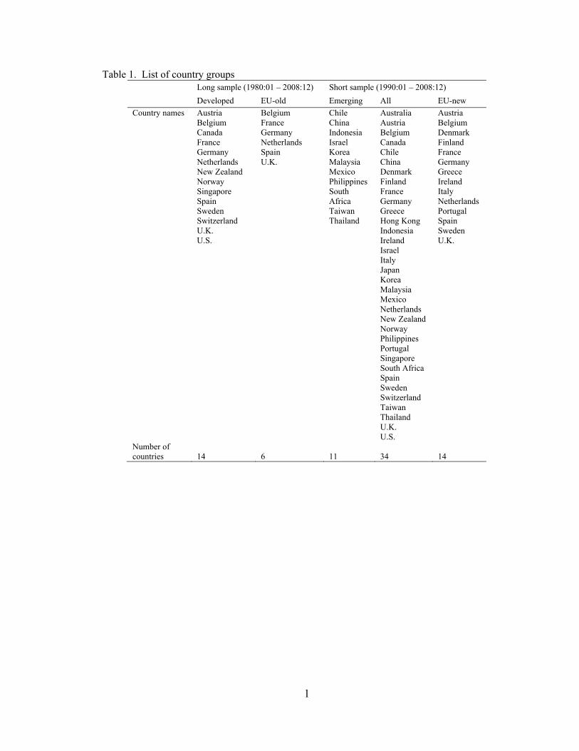
1

Table 1. List of country groups Long sample (1980:01 – 2008:12) Short sample (1990:01 – 2008:12)

Developed EU-old Emerging All EU-new

Country names Austria Belgium Canada France Germany Netherlands New Zealand Norway Singapore Spain Sweden Switzerland U.K. U.S.

Belgium France Germany Netherlands Spain U.K.

Chile China Indonesia Israel Korea Malaysia Mexico Philippines South Africa Taiwan Thailand

Australia Austria Belgium Canada Chile China Denmark Finland France Germany Greece Hong Kong Indonesia Ireland Israel Italy Japan Korea Malaysia Mexico Netherlands New Zealand Norway Philippines Portugal Singapore South Africa Spain Sweden Switzerland Taiwan Thailand U.K. U.S.

Austria Belgium Denmark Finland France Germany Greece Ireland Italy Netherlands Portugal Spain Sweden U.K.

Number of countries 14 6 11 34 14

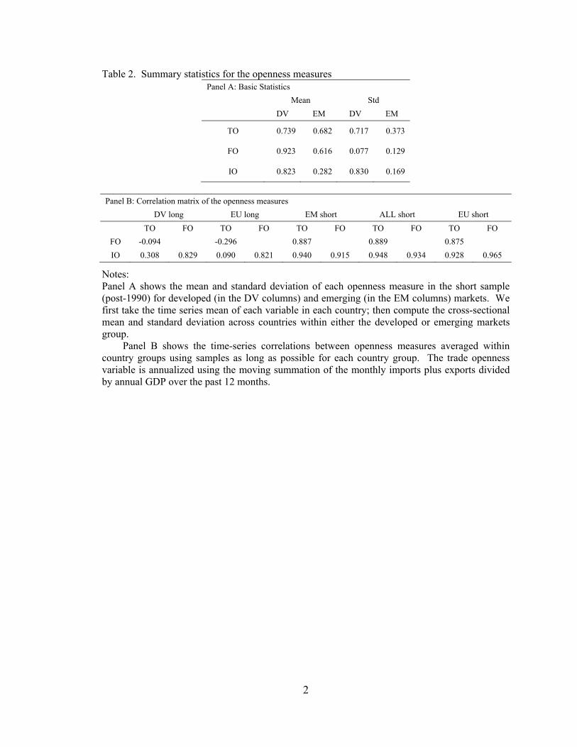
2

Table 2. Summary statistics for the openness measures Panel A: Basic Statistics

Mean Std

DV EM DV EM

TO 0.739 0.682 0.717 0.373

FO 0.923 0.616 0.077 0.129

IO 0.823 0.282 0.830 0.169

Panel B: Correlation matrix of the openness measures

DV long EU long EM short ALL short EU short

TO FO TO FO TO FO TO FO TO FO

FO -0.094 -0.296 0.887 0.889 0.875

IO 0.308 0.829 0.090 0.821 0.940 0.915 0.948 0.934 0.928 0.965

Notes: Panel A shows the mean and standard deviation of each openness measure in the short sample (post-1990) for developed (in the DV columns) and emerging (in the EM columns) markets. We first take the time series mean of each variable in each country; then compute the cross-sectional mean and standard deviation across countries within either the developed or emerging markets group. Panel B shows the time-series correlations between openness measures averaged within country groups using samples as long as possible for each country group. The trade openness variable is annualized using the moving summation of the monthly imports plus exports divided by annual GDP over the past 12 months.

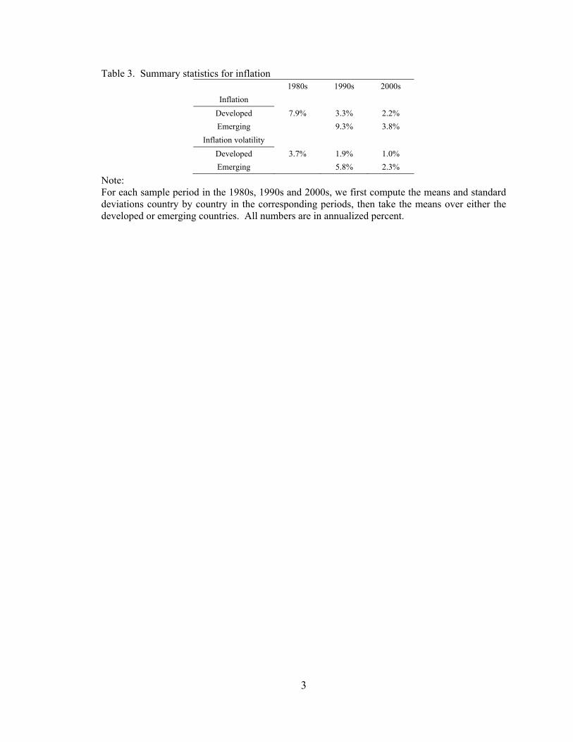
3

Table 3. Summary statistics for inflation

Note: For each sample period in the 1980s, 1990s and 2000s, we first compute the means and standard deviations country by country in the corresponding periods, then take the means over either the developed or emerging countries. All numbers are in annualized percent.

1980s 1990s 2000s

Inflation

Developed 7.9% 3.3% 2.2%

Emerging 9.3% 3.8%

Inflation volatility

Developed 3.7% 1.9% 1.0%

Emerging 5.8% 2.3%

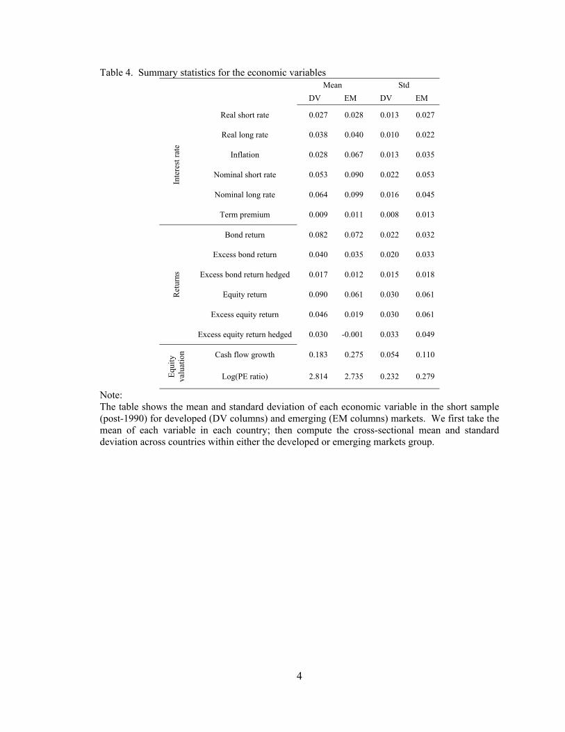
4

Table 4. Summary statistics for the economic variables Mean Std

DV EM DV EM

Inte

rest

rat

e

Real short rate 0.027 0.028 0.013 0.027

Real long rate 0.038 0.040 0.010 0.022

Inflation 0.028 0.067 0.013 0.035

Nominal short rate 0.053 0.090 0.022 0.053

Nominal long rate 0.064 0.099 0.016 0.045

Term premium 0.009 0.011 0.008 0.013

Ret

urns

Bond return 0.082 0.072 0.022 0.032

Excess bond return 0.040 0.035 0.020 0.033

Excess bond return hedged 0.017 0.012 0.015 0.018

Equity return 0.090 0.061 0.030 0.061

Excess equity return 0.046 0.019 0.030 0.061

Excess equity return hedged 0.030 -0.001 0.033 0.049

Equ

ity

valu

atio

n Cash flow growth 0.183 0.275 0.054 0.110

Log(PE ratio) 2.814 2.735 0.232 0.279

Note: The table shows the mean and standard deviation of each economic variable in the short sample (post-1990) for developed (DV columns) and emerging (EM columns) markets. We first take the mean of each variable in each country; then compute the cross-sectional mean and standard deviation across countries within either the developed or emerging markets group.

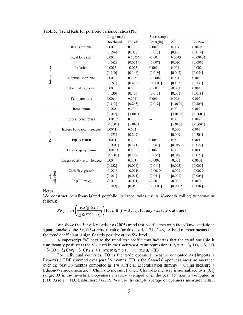
5

Table 5. Trend tests for portfolio variance ratios (PR) Long sample Short sample Developed EU-old Emerging All EU-new

Inte

rest

rat

es

Real short rate 0.002 0.001 0.002 0.005 0.0003

[0.194] [0.038] [0.013] [0.195] [0.014]

Real long rate 0.001 0.0003ª -0.001 0.0003 -0.00002

[0.062] [0.005] [0.007] [0.030] [0.0002]

Inflation 0.0005 -0.003 0.001 0.004 -0.002

[0.010] [0.146] [0.019] [0.047] [0.055]

Nominal short rate 0.003 0.002 -0.0002 0.004 0.003

[0.191] [0.415] [<.0001] [0.103] [0.137]

Nominal long rate 0.003 0.001 -0.003 -0.001 0.004

[0.130] [0.406] [0.013] [0.001] [0.019]

Term premium 0.006 0.006ª 0.001 0.003 0.005ª

[0.313] [0.245] [0.012] [<.0001] [0.209]

Ret

urns

Bond return -0.0001 0.001 -- 0.001 0.002

[0.002] [<.0001] [<.0001] [<.0001]

Excess bond return 0.00002 0.001 -- 0.001 0.002

[<.0001] [<.0001] [<.0001] [<.0001]

Excess bond return hedged 0.0001 0.002 -- -0.0001 0.002

[0.023] [0.247] [0.009] [0.305]

Equity return 0.0001 0.001 0.003 0.001 0.001

[0.0001] [0.121] [0.083] [0.019] [0.022]

Excess equity return 0.00003 0.001 0.002 0.001 0.001

[<.0001] [0.112] [0.055] [0.012] [0.022]

Excess equity return hedged 0.001 0.003 -0.0003 -0.001 0.0002

[0.032] [0.019] [0.011] [0.003] [0.003]

Equ

ity

valu

atio

n Cash flow growth -0.001ª -0.001ª -0.0030ª -0.002 -0.0029

[0.001] [0.001] [0.041] [0.002] [0.009]

Log(PE ratio) -0.001 -0.001 -0.001 -0.002 0.000

[0.089] [0.053] [<.0001] [0.0002] [0.004]

Notes: We construct equally-weighted portfolio variance ratios using 36-month rolling windows as follows:

∑ ,

∑ ,

for 35, , for any variable x at time t.

We show the Bunzel-Vogelsang (2005) trend test coefficients with the t-Dan-J statistic in square brackets; the 5% (1%) critical value for this test is 1.71 (2.46). A bold number means that the trend coefficient is significantly positive at the 5% level.

A superscript “a” next to the trend test coefficients indicates that the trend variable is significantly positive at the 5% level in the Cochrane-Orcutt regression: PRt = α + β1 TOt + β2 FOt + β3 IOt + β4 Cyct + β5 Crisist + εt where εt = ρ εt-1 + ut and ut ~ IID.

For individual countries, TO is the trade openness measure computed as (Imports + Exports) / GDP summed over past 36 months; FO is the financial openness measure averaged over the past 36 months computed as 1/4 (Official Liberalization dummy + Quinn measure + Edison-Warnock measure + Chinn-Ito measure) where Chinn-Ito measure is normalized to a [0,1] range; IO is the investment openness measure averaged over the past 36 months computed as (FDI Assets + FDI Liabilities) / GDP. We use the simple average of openness measures within

6

the country groups in the PR regressions. We also control for world business cycle and crisis effects in the openness regression. The monthly variable Cyct is constructed using a weighted average of the annual world business cycle variable Cycs,a in the current year and last year. The annual business cycle variable is computed by subtracting a moving average of world GDP growth (over the last 5 years) from current GDP growth. Crisist is the sum of the dummy variable Crisisi,t over all the countries in a particular country group, where Crisisi,t takes a value of 1 when there is a banking/economic crisis in country i at time t and 0 otherwise according to Caprio and Klingebiel (2003) and Reinhart and Rogoff (2008).

The missing values for the emerging markets group’s bond return related variables are due to the short history of the emerging markets data. Because of the 36-month window needed to compute the portfolio variance ratios, the sample drops to less than 6 observations.

7

Table 6. Multi-variate regression of portfolio variance ratios (PR) Long sample

Developed EU-old

TO FO IO TO FO IO

Inte

rest

rat

e

Real short rate 0.57 16.40*** -0.29 0.13 4.77 0.18

Real long rate 1.36*** 22.26*** -1.84** 0.40* 4.32 -0.71*

Inflation -0.41 -10.76* 1.32* 0.32 -5.41 -0.26

Nominal short rate -1.68*** 5.35 2.07** 0.34 9.17*** -0.25

Nominal long rate -2.36*** 5.20 1.42** 0.04 6.61*** -0.30*

Term premium 1.90*** -2.70 -0.26 0.14 -3.00 1.25**

Ret

urns

Bond return 0.25 -7.09*** 0.47* 0.18*** -1.33 0.29**

Excess bond return 0.45** -5.31* 0.25 0.27*** -2.27** 0.34***

Excess bond return hedged 0.09 0.13 0.23 0.31* 17.09*** -1.33***

Equity return -0.32 -2.95 0.24 0.05 4.20** -0.38*

Excess equity return -0.48 -4.03 0.40 -0.03 2.12 -0.17

Excess equity return hedged 0.15 -4.61* -0.04 -0.65*** -2.72** 0.58***

Equ

ity

valu

atio

n Cash flow growth 1.22** 20.53*** -1.75* 0.16 2.60 -0.35

Log(PE ratio) -1.56*** -15.89*** 1.61*** -0.62*** -9.39*** 0.77**

8

Table 6. Multi-variate regression of portfolio variance ratios (PR) (continued) Short sample

Emerging All EU-new

TO FO IO TO FO IO TO FO IO

Inte

rest

rat

e

Real short rate 0.81** -1.30 -2.85 1.36** 8.21** -1.85** -0.41 1.03 0.44

Real long rate 0.67 12.06** -5.97** 1.81** 4.20** -2.62*** 3.60*** 8.80*** -3.42***

Inflation 0.57* -1.61 0.22 1.29 -1.39 -1.03 -0.13 -3.67* 0.17

Nominal short rate 0.34 5.51*** -7.83*** 0.95* 9.83*** -1.41** 1.19** 5.80** -0.78

Nominal long rate -2.34*** 2.37 3.63 -2.47*** 10.64*** -0.37 -0.68 4.16** 0.42

Term premium 1.43** -12.66** 4.80* 1.30** 7.05** -1.82** 0.58 6.19*** -0.18

Ret

urns

Bond return -- -- -- 0.09 -5.00*** 0.80** 0.47** -0.12 0.25

Excess bond return -- -- -- 0.35 -8.27*** 0.52 0.60** -0.15 0.21

Excess bond return hedged -- -- -- 0.15 -0.54 0.28 0.93** -3.62 0.41

Equity return -3.62*** 10.65** 6.51** -1.54** -2.26* 1.74** -1.37*** -3.55** 1.15**

Excess equity return -3.34*** 9.39** 6.12** -1.58** -1.99 1.59** -1.55*** -4.22** 1.31**

Excess equity return hedged -1.69** -1.70 6.22** -0.89 -0.09 0.31 -1.07** -1.11 0.39

Equ

ity

valu

atio

n Cash flow growth -0.60 -17.12*** 15.18*** 0.97 -1.52 -0.60 0.61 3.24 -1.15*

Log(PE ratio) -3.46*** 16.13** 3.98 -1.23** -5.23*** 1.37* -0.24 -7.36** 0.688

Notes: We report the results of the multivariate regression using the Cochrane-Orcutt method: PRt = α + β1 TOt + β2 FOt + β3 IOt + β4 Cyct + β5 Crisist + εt where εt = ρ εt-1 + ut and ut ~ IID. We report the coefficients on the openness measures with * indicating coefficients significant at the 10% level; ** indicating coefficients significant at the 5% level; *** indicating coefficients significant at the 1% level.

The missing values for the emerging markets group’s bond return related variables are due to the short history of the emerging markets data. Because of the 36-month window needed to compute the portfolio variance ratios, the sample drops to less than 6 observations.

For the construction of all other variables, see the notes to Table 5.

9

Table 7. Multivariate beta models Panel A: With respect to the world benchmark

Long sample

Developed EU-old

TO FO IO TO FO IO

Inte

rest

rat

e Real short rate 0.74* 0.44** -0.08 1.23** 0.42** 0.09

Real long rate 0.55 0.13 0.05 0.38 0.45** 0.05

Inflation -0.03 -0.05 0.06** 0.20*** 0.30*** 0.09***

Nominal short rate 0.02 0.72*** -0.22*** 0.03 0.44*** -0.17**

Nominal long rate -0.17 0.41*** -0.09** 0.18 0.48*** -0.19***

Term premium -0.21 0.44** 0.27*** -0.47 0.89** 0.57***

Ret

urns

Bond return -0.89** 0.78*** 0.03* -0.65* 0.08 0.03

Excess bond return -0.96** 0.71*** 0.03 -0.85** -0.03 0.02

Excess bond return hedged 1.86*** 0.57** 0.18*** -0.28 0.31 0.11**

Equity return 0.63* 0.17 -0.01 0.13 0.06 -0.04

Excess equity return 0.56* 0.16 -0.01 0.04 0.05 -0.04

Excess equity return hedged 0.87** 0.14 0.04 0.40 0.33** 0.11***

Equ

ity

valu

atio

n Cash flow growth 0.83* 0.82** 0.24*** 0.60 -0.31 0.13**

Log(PE ratio) 0.26 -0.56** 0.05 -1.45** -0.76*** 0.01

10

Table 7. Multivariate beta models (continued) Panel A: With respect to the world benchmark (continued)

Short sample

Emerging All EU-new

TO FO IO TO FO IO TO FO IO

Inte

rest

rat

e

Real short rate 4.01 0.57 2.68** 1.39* 0.51* -0.25** 3.22** -3.66*** -0.72***

Real long rate 3.66* 0.38 0.25 1.05 0.56** 0.09 0.50 0.64* 0.00

Inflation -0.09 0.18*** 0.83*** 0.05 0.19*** 0.11*** 0.16*** 0.22** 0.30***

Nominal short rate 0.61 -0.15 2.08** 0.35 0.24 -0.12* 1.61** 1.13*** -0.25***

Nominal long rate -0.60 -0.27 -0.77 -0.29 -0.17 -0.03 -0.37 0.47** -0.08*

Term premium 1.25 -0.43 -0.02 -0.85 0.04 -0.47*** -3.37 1.61* -0.85***

Ret

urns

Bond return 1.31 -1.12** 2.73*** -0.68 0.27* 0.02 -0.41 0.04 -0.01

Excess bond return 1.03 -0.92* 2.68*** -0.62 0.30* 0.02 -0.29 0.01 -0.01

Excess bond return hedged 3.04* 0.36 -0.30 1.78*** 0.43** 0.22*** -0.02 1.02*** 0.22***

Equity return 0.59 0.29 0.71** 0.22 0.07 -0.01 1.54** -0.59** 0.02

Excess equity return 0.59 0.28 0.71** 0.21 0.07 -0.01 1.48** -0.58** 0.01

Excess equity return hedged 0.01 -0.42* -0.17 0.18 -0.51*** -0.07** 0.72 -0.61** 0.05

Equ

ity

valu

atio

n Cash flow growth -2.51 0.17 2.49*** 0.61 0.40* 0.15** 1.29 0.66 0.21**

Log(PE ratio) 0.68 -0.34 0.30 0.37 -0.37** 0.01 -1.25 -0.40 0.03

11

Table 7. Multivariate beta models (continued) Panel B: With respect to the U.S. benchmark

Long sample

Developed EU-old

TO FO IO TO FO IO

Inte

rest

rat

e Real short rate 0.74** 0.54*** 0.07** 0.92** 0.48*** 0.07**

Real long rate -0.56* 0.63*** 0.10*** -0.39 0.40*** 0.02

Inflation -0.04 0.10 0.02 0.70** -0.02 0.03

Nominal short rate 0.54** 0.52*** 0.11** 0.88** 0.36** 0.07

Nominal long rate 0.01 1.11*** 0.24*** 0.64** 1.24*** 0.15***

Term premium 0.47 0.59*** 0.31*** -0.33 0.65*** 0.36***

Ret

urns

Bond return -4.79*** 1.41*** 0.29*** -4.73** 1.05* 0.24**

Excess bond return -6.71*** 1.52*** 0.36*** -6.53*** 1.14* 0.30***

Excess bond return hedged -1.46** 0.89*** 0.26*** -0.66 0.67*** 0.23***

Equity return 1.83*** 1.29*** 0.11*** 1.62* 1.20*** 0.11**

Excess equity return 1.71*** 1.29*** 0.12*** 1.42 1.20*** 0.12**

Excess equity return hedged 1.03* 1.22*** 0.19*** 0.06 1.24*** 0.24***

Equ

ity

valu

atio

n Cash flow growth -0.69 1.63** 0.54*** -1.20 2.19** 0.53***

Log(PE ratio) -0.58** -0.20 0.10** -2.28*** -0.39* 0.05

12

Table 7. Multivariate beta models (continued) Panel B: With respect to the U.S. benchmark (continued)

Short sample

Emerging All EU-new

TO FO IO TO FO IO TO FO IO

Inte

rest

rat

e

Real short rate -1.94 0.54 0.21 -1.02 0.56* 0.06 -0.36 0.98* 0.05

Real long rate 2.30 0.80* 0.01 0.69 0.77*** 0.04 -2.21*** -0.01 -0.09**

Inflation -2.26 -0.02 -1.52*** -0.25 0.07 0.01 1.03 -0.03 -0.003

Nominal short rate -2.17 0.13 0.67 -0.46 0.44 0.13 0.46 1.59** 0.22**

Nominal long rate -0.37 1.06** 0.29 -0.29 1.10*** 0.01 -1.09** 1.47*** -0.02

Term premium -0.05 -0.12 0.11 1.09 0.31 0.54*** 4.15** 3.39*** 0.85***

Ret

urns

Bond return 6.37* -0.28 -3.25* -0.08 1.67*** 0.47*** -0.16 3.31*** 0.57***

Excess bond return 5.64 0.04 -2.21 -0.82 1.98*** 0.58*** -0.32 3.75*** 0.68***

Excess bond return hedged -2.15 -0.35 -0.93 -1.80*** 0.43** 0.24*** 1.05 1.32*** 0.27***

Equity return 0.16 0.76** 0.96** 1.35** 1.02*** 0.09** 3.59*** 2.48*** 0.20***

Excess equity return 0.17 0.77** 0.98** 1.31** 1.03*** 0.09** 3.58*** 2.51*** 0.20***

Excess equity return hedged 0.35 0.36 0.63* 0.98* 0.61*** 0.06 1.58* 1.80*** 0.16***

Equ

ity

valu

atio

n Cash flow growth -2.98 1.20* 2.88*** -1.15 1.71*** 0.31*** -1.78 4.23*** 0.27**

Log(PE ratio) 1.05 -0.24 0.73* 0.64 -0.23 -0.05 0.17 -0.04 -0.083

Notes: We estimate the following panel factor model: xi,t = αi + αopen Openi,t + αrec Cyct + αcri Crisisi,t + (γi + γopen Openi,t + γcyc Cyct + γcri Crisisi,t) xglob,t + εi,t where Openi,t is either TOi,t, FOi,t or IOi,t; xglob,t takes two forms, , or xUS,t. Crisisi,t is the dummy taking a value of 1 when there is a banking/economic crisis in country i at time t and 0 otherwise according to Caprio and Klingebiel (2003) and Reinhart and Rogoff (2008). Other variables are constructed in the same way as before. The regressions are estimated using the Cochrane-Orcutt method, where εi,t = ρi εi,t-1 + ui,t and ui,t ~ IID.

For each country group, we report the γopen coefficients, with * indicating significance at the 10% level; ** indicating significance at the 5% level; *** indicating significance at the 1% level.

For the construction of all other variables, see the notes to Table 5.

13

Table 8. Trend tests for country effect standard deviation (CESD) Long sample Short sample Developed EU-old Emerging All EU-new

Inte

rest

rat

es

Real short rate -0.00003ª 0.000002 -0.00016ª -0.00005 0.00004

[1.665] [0.177] [0.276] [0.200] [1.246]

Real long rate -0.00001ª 0.000005 0.00004 0.00002 -0.00002ª

[0.991] [0.347] [0.081] [0.072] [0.029]

Inflation -0.00006ª -0.00008ª -0.00033 -0.00023 -0.00017ª

[0.079] [<.0001] [0.319] [0.406] [<.0001]

Nominal short rate 0.000001 0.00001 -0.00027ª -0.00014 -0.00009ª

[0.015] [0.041] [0.727] [0.350] [4.659]

Nominal long rate -0.00001ª -0.00002ª -0.00005ª -0.00009ª -0.00013ª

[0.0005] [0.260] [0.319] [1.037] [<.0001]

Term premium -0.00004ª -0.00005ª -0.00004ª -0.00009 -0.00011

[1.933] [0.004] [0.316] [1.436] [1.803]

Ret

urns

Bond return -0.00005ª -0.00008ª 0.00201 -0.00004ª -0.00012ª

[1.398] [1.859] [0.002] [0.472] [2.073]

Excess bond return -0.00005ª -0.00012ª 0.00152 -0.00002ª -0.00013ª

[1.106] [1.615] [0.0004] [0.153] [1.199]

Excess bond return hedged -0.00002 -0.00007ª 0.00093 -0.00002 -0.00014

[0.418] [2.938] [0.001] [0.018] [0.111]

Equity return -0.00020ª -0.00020ª -0.00116 -0.00074 -0.00050

[0.584] [0.637] [0.715] [0.137] [0.038]

Excess equity return -0.00024ª -0.00024ª -0.00115 -0.00071 -0.00046

[0.614] [0.660] [0.807] [0.137] [0.051]

Excess equity return hedged -0.00023ª -0.00021ª -0.00092 -0.00055 -0.00045

[0.808] [0.664] [0.352] [0.033] [0.054]

Equ

ity

valu

atio

n Cash flow growth -0.00001 -0.00017 -0.00126ª -0.00070 -0.00090ª

[0.028] [0.128] [0.172] [0.232] [0.357]

Log(PE ratio) -0.00028ª -0.00024ª 0.00018 0.00001ª -0.00012ª

[<.0001] [<.0001] [<.0001] [<.0001] [<.0001]

Notes: We construct the equally-weighted country effect standard deviation measure as follows:

∑ , where µ and gt are from Cochrane-Orcutt estimation of the

regression: xi,t = µ + gt + αi + ei,t We show the Bunzel-Vogelsang (2005) trend test coefficients with the t-Dan-J statistic in

square brackets; the 5% (1%) critical value for this test is 1.71 (2.46). A bold number means that the trend coefficient is significant at the 5% level.

A superscript “a” next to the trend test coefficients indicates that the trend variable is negatively significant at the 5% level in the Cochrane-Orcutt regression: CESDt = α + β1 TOt + β2 FOt + β3 IOt + γ t + β4 Cyct + β5 Crisist + εt where εt = ρ εt-1 + ut and ut ~ IID.

For the construction of all other variables, see the notes to Table 5.

14

Table 9. Multi-variate regression of country effect standard deviation (CESD) Long sample

Developed EU-old

TO FO IO TO FO IO

Inte

rest

rat

e

Real short rate 0.003 0.02 -0.01*** -0.01 -0.04*** 0.004**

Real long rate 0.02* 0.02* -0.004** 0.004 0.01** -0.0003

Inflation 0.01 0.01 -0.01** 0.02 -0.06*** -0.003**

Nominal short rate 0.004 -0.06*** 0.01*** -0.01 -0.07*** 0.007***

Nominal long rate -0.0001 0.01 -0.001 -0.002 -0.003 -0.001***

Term premium -0.02 -0.001 -0.01*** -0.03** 0.002 -0.01**

Ret

urns

Bond return -0.01 0.01 -0.01* -0.01 0.02 -0.02*

Excess bond return 0.03 0.019 -0.02* -0.04 0.06 -0.03*

Excess bond return hedged 0.09* 0.02 -0.01* 0.03 -0.01 -0.01*

Equity return -0.24 -0.17 -0.002 0.15 0.07 -0.03*

Excess equity return -0.24 -0.20 -0.003 0.21 0.07 -0.03*

Excess equity return hedged -0.17 -0.21 -0.01 0.24 0.11 -0.04**

Equ

ity

valu

atio

n Cash flow growth -0.09 -0.71*** 0.07* -0.07 0.01 -0.01

Log(PE ratio) -0.03 0.04 -0.06*** 0.03 0.003 -0.04***

15

Table 9. Multi-variate regression of country effect standard deviation (CESD) (continued) Short sample

Emerging All EU-new

TO FO IO TO FO IO TO FO IO

Inte

rest

rat

e

Real short rate 0.31** 0.08 -0.054 0.03 0.14 -0.03* -0.06 -0.19** 0.04***

Real long rate 0.21* 0.16** -0.01 0.09 0.14* -0.02 0.01 -0.02 0.0003

Inflation 0.05 -0.01 -0.05 -0.02 -0.04 -0.01 -0.004 -0.03 -0.001

Nominal short rate 0.09 -0.03 -0.02 0.02 0.02 -0.01 -0.06 -0.04 -0.01*

Nominal long rate 0.07 0.04 0.002 0.04 -0.02 -0.01 -0.005 -0.03 -0.002

Term premium 0.02 0.02 -0.04* -0.11* 0.02 -0.02** -0.12* -0.05 -0.01

Ret

urns

Bond return -0.23 0.22 -0.51 -0.24* 0.07 -0.01 0.08 -0.10 -0.01

Excess bond return -0.77** 0.77* 0.06 -0.29* 0.15 -0.02 0.09 -0.16 -0.005

Excess bond return hedged -0.08 0.08 -0.05 0.09 -0.06 0.001 0.004 -0.07 -0.01

Equity return 0.46 -0.02 -0.54** -0.16 -0.10 -0.10 -0.19 -0.79* 0.10

Excess equity return 0.41 0.00 -0.57** -0.15 -0.09 -0.11 -0.18 -0.92* 0.12*

Excess equity return hedged -0.13 -0.14 -0.32* -0.26 -0.35 -0.03 -0.48 -1.15** 0.14*

Equ

ity

valu

atio

n Cash flow growth -1.00 0.20 -0.10 -0.79 0.35 -0.09 -0.71** -0.68 0.02

Log(PE ratio) 0.39** 0.22*** 0.09 0.09 0.02 -0.01 -0.07 -0.19 -0.01

Notes: We report the results of the multivariate regression using the Cochrane-Orcutt method: CESDt = α + β1 TOt + β2 FOt + β3 IOt + β4 Cyct + β5 Crisist + εt where εt = ρ εt-1 + ut and ut ~ IID. We report the coefficients on the openness measures with * indicating coefficients significant at the 10% level; ** indicating coefficients significant at the 5% level; *** indicating coefficients significant at the 1% level.

For the construction of all other variables, see the notes to Table 5.

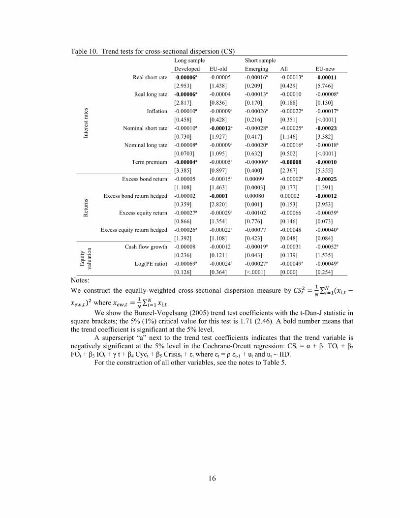
16

Table 10. Trend tests for cross-sectional dispersion (CS) Long sample Short sample Developed EU-old Emerging All EU-new

Inte

rest

rat

es

Real short rate -0.00006ª -0.00005 -0.00016ª -0.00013ª -0.00011

[2.953] [1.438] [0.209] [0.429] [5.746]

Real long rate -0.00006ª -0.00004 -0.00013ª -0.00010 -0.00008ª

[2.817] [0.836] [0.170] [0.188] [0.130]

Inflation -0.00010ª -0.00009ª -0.00026ª -0.00022ª -0.00017ª

[0.458] [0.428] [0.216] [0.351] [<.0001]

Nominal short rate -0.00010ª -0.00012ª -0.00028ª -0.00025ª -0.00023

[0.730] [1.927] [0.417] [1.146] [3.382]

Nominal long rate -0.00008ª -0.00009ª -0.00020ª -0.00016ª -0.00018ª

[0.0703] [1.095] [0.632] [0.502] [<.0001]

Term premium -0.00004ª -0.00005ª -0.00006ª -0.00008 -0.00010

[3.385] [0.897] [0.400] [2.367] [5.355]

Ret

urns

Excess bond return -0.00005 -0.00015ª 0.00099 -0.00002ª -0.00025

[1.108] [1.463] [0.0003] [0.177] [1.391]

Excess bond return hedged -0.00002 -0.0001 0.00080 0.00002 -0.00012

[0.359] [2.820] [0.001] [0.153] [2.953]

Excess equity return -0.00027ª -0.00029ª -0.00102 -0.00066 -0.00039ª

[0.866] [1.354] [0.776] [0.146] [0.073]

Excess equity return hedged -0.00026ª -0.00022ª -0.00077 -0.00048 -0.00040ª

[1.392] [1.108] [0.423] [0.048] [0.084]

Equ

ity

valu

atio

n Cash flow growth -0.00008 -0.00012 -0.00019ª -0.00031 -0.00052ª

[0.236] [0.121] [0.043] [0.139] [1.535]

Log(PE ratio) -0.00069ª -0.00024ª -0.00027ª -0.00049ª -0.00049ª

[0.126] [0.364] [<.0001] [0.000] [0.254]

Notes:

We construct the equally-weighted cross-sectional dispersion measure by ∑ ,

, where , ∑ ,

We show the Bunzel-Vogelsang (2005) trend test coefficients with the t-Dan-J statistic in square brackets; the 5% (1%) critical value for this test is 1.71 (2.46). A bold number means that the trend coefficient is significant at the 5% level.

A superscript “a” next to the trend test coefficients indicates that the trend variable is negatively significant at the 5% level in the Cochrane-Orcutt regression: CSt = α + β1 TOt + β2 FOt + β3 IOt + γ t + β4 Cyct + β5 Crisist + εt where εt = ρ εt-1 + ut and ut ~ IID.

For the construction of all other variables, see the notes to Table 5.

17

Table 11. Multi-variate regression of cross-sectional dispersion (CS) Long sample

Developed EU-old

TO FO IO TO FO IO

Inte

rest

rat

e

Real short rate 0.002 0.02 -0.02*** -0.01 -0.04** -0.01*

Real long rate 0.02 0.01 -0.01*** 0.01 -0.02* -0.002

Inflation 0.02 0.02 -0.01** 0.01 -0.03** -0.01***

Nominal short rate -0.01 -0.07*** -0.01*** -0.02 -0.10*** -0.01*

Nominal long rate -0.01 0.001 -0.01*** -0.002 -0.02** -0.01***

Term premium -0.03* 0.005 -0.01*** -0.03* 0.001 -0.01***

Ret

urns

Excess bond return 0.08 0.001 -0.01 -0.11 0.10 -0.04*

Excess bond return hedged 0.11* -0.05 -0.003 0.01 0.04 -0.02**

Excess equity return -0.24 -0.15 -0.012 0.24 -0.08 -0.03

Excess equity return hedged -0.24 -0.24* -0.01 0.24 0.02 -0.04**

Equ

ity

valu

atio

n Cash flow growth -0.02 -0.68** 0.07* -0.06 -0.05 -0.01

Log(PE ratio) -0.06 -1.09*** 0.02 0.26 -0.37*** 0.02

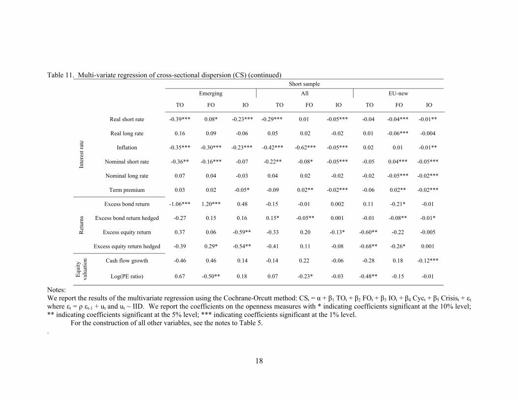
18

Table 11. Multi-variate regression of cross-sectional dispersion (CS) (continued) Short sample

Emerging All EU-new

TO FO IO TO FO IO TO FO IO

Inte

rest

rat

e

Real short rate -0.39*** 0.08* -0.23*** -0.29*** 0.01 -0.05*** -0.04 -0.04*** -0.01**

Real long rate 0.16 0.09 -0.06 0.05 0.02 -0.02 0.01 -0.06*** -0.004

Inflation -0.35*** -0.30*** -0.23*** -0.42*** -0.62*** -0.05*** 0.02 0.01 -0.01**

Nominal short rate -0.36** -0.16*** -0.07 -0.22** -0.08* -0.05*** -0.05 0.04*** -0.05***

Nominal long rate 0.07 0.04 -0.03 0.04 0.02 -0.02 -0.02 -0.05*** -0.02***

Term premium 0.03 0.02 -0.05* -0.09 0.02** -0.02*** -0.06 0.02** -0.02***

Ret

urns

Excess bond return -1.06*** 1.20*** 0.48 -0.15 -0.01 0.002 0.11 -0.21* -0.01

Excess bond return hedged -0.27 0.15 0.16 0.15* -0.05** 0.001 -0.01 -0.08** -0.01*

Excess equity return 0.37 0.06 -0.59** -0.33 0.20 -0.13* -0.60** -0.22 -0.005

Excess equity return hedged -0.39 0.29* -0.54** -0.41 0.11 -0.08 -0.68** -0.26* 0.001

Equ

ity

valu

atio

n Cash flow growth -0.46 0.46 0.14 -0.14 0.22 -0.06 -0.28 0.18 -0.12***

Log(PE ratio) 0.67 -0.50** 0.18 0.07 -0.23* -0.03 -0.48** -0.15 -0.01

Notes: We report the results of the multivariate regression using the Cochrane-Orcutt method: CSt = α + β1 TOt + β2 FOt + β3 IOt + β4 Cyct + β5 Crisist + εt where εt = ρ εt-1 + ut and ut ~ IID. We report the coefficients on the openness measures with * indicating coefficients significant at the 10% level; ** indicating coefficients significant at the 5% level; *** indicating coefficients significant at the 1% level.

For the construction of all other variables, see the notes to Table 5. .

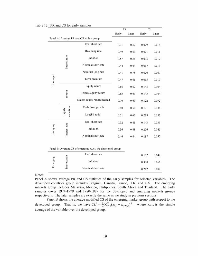
19

Table 12. PR and CS for early samples PR CS

Early Later Early Later

Panel A: Average PR and CS within group

Dev

elop

ed

Inte

rest

rat

e

Real short rate 0.31 0.57 0.029 0.014

Real long rate 0.49 0.63 0.021 0.011

Inflation 0.57 0.56 0.033 0.012

Nominal short rate 0.44 0.64 0.017 0.013

Nominal long rate 0.41 0.78 0.020 0.007

Term premium 0.47 0.61 0.015 0.010

retu

rns

Equity return 0.66 0.62 0.145 0.104

Excess equity return 0.65 0.63 0.145 0.104

Excess equity return hedged 0.70 0.69 0.122 0.092

Equ

ity

valu

atio

n Cash flow growth 0.40 0.50 0.171 0.134

Log(PE ratio) 0.51 0.63 0.218 0.152

Em

ergi

ng

Inte

rest

rat

e Real short rate 0.32 0.41 0.143 0.039

Inflation 0.36 0.48 0.256 0.045

Nominal short rate 0.46 0.44 0.187 0.057

Panel B: Average CS of emerging w.r.t. the developed group

Em

ergi

ng

Inte

rest

rat

e Real short rate 0.172 0.048

Inflation 0.300 0.066

Nominal short rate 0.212 0.082

Notes: Panel A shows average PR and CS statistics of the early samples for selected variables. The developed countries group includes Belgium, Canada, France, U.K. and U.S. The emerging markets group includes Malaysia, Mexico, Philippines, South Africa and Thailand. The early samples cover 1974-1979 and 1980-1989 for the developed and emerging markets groups respectively. The later samples are exactly the same as we study in previous sections.

Panel B shows the average modified CS of the emerging market group with respect to the

developed group. That is, we have CSN

∑ x , x ,N . where xdev,t is the simple

average of the variable over the developed group.

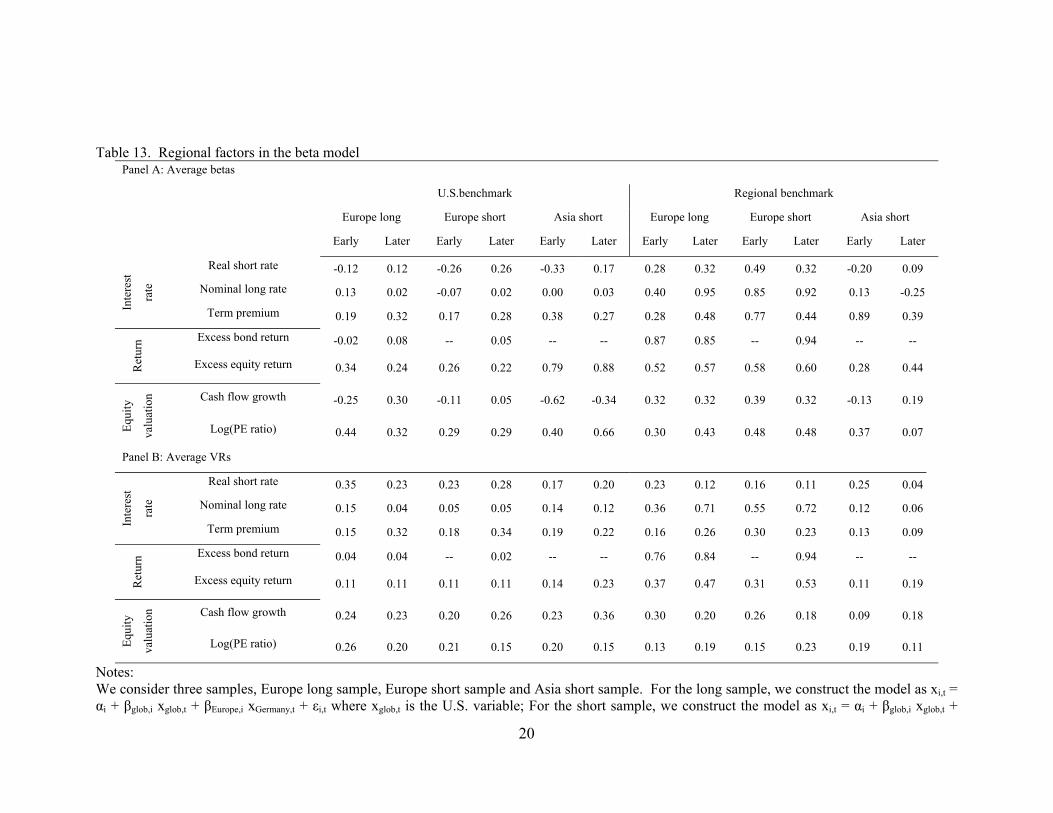
20

Table 13. Regional factors in the beta model Panel A: Average betas

U.S.benchmark Regional benchmark

Europe long Europe short Asia short Europe long Europe short Asia short

Early Later Early Later Early Later Early Later Early Later Early Later

Inte

rest

rate

Real short rate -0.12 0.12 -0.26 0.26 -0.33 0.17 0.28 0.32 0.49 0.32 -0.20 0.09

Nominal long rate 0.13 0.02 -0.07 0.02 0.00 0.03 0.40 0.95 0.85 0.92 0.13 -0.25

Term premium 0.19 0.32 0.17 0.28 0.38 0.27 0.28 0.48 0.77 0.44 0.89 0.39

Ret

urn Excess bond return -0.02 0.08 -- 0.05 -- -- 0.87 0.85 -- 0.94 -- --

Excess equity return 0.34 0.24 0.26 0.22 0.79 0.88 0.52 0.57 0.58 0.60 0.28 0.44

Equ

ity

valu

atio

n Cash flow growth -0.25 0.30 -0.11 0.05 -0.62 -0.34 0.32 0.32 0.39 0.32 -0.13 0.19

Log(PE ratio) 0.44 0.32 0.29 0.29 0.40 0.66 0.30 0.43 0.48 0.48 0.37 0.07

Panel B: Average VRs

Inte

rest

rate

Real short rate 0.35 0.23 0.23 0.28 0.17 0.20 0.23 0.12 0.16 0.11 0.25 0.04

Nominal long rate 0.15 0.04 0.05 0.05 0.14 0.12 0.36 0.71 0.55 0.72 0.12 0.06

Term premium 0.15 0.32 0.18 0.34 0.19 0.22 0.16 0.26 0.30 0.23 0.13 0.09

Ret

urn

Excess bond return 0.04 0.04 -- 0.02 -- -- 0.76 0.84 -- 0.94 -- --

Excess equity return 0.11 0.11 0.11 0.11 0.14 0.23 0.37 0.47 0.31 0.53 0.11 0.19

Equ

ity

valu

atio

n Cash flow growth 0.24 0.23 0.20 0.26 0.23 0.36 0.30 0.20 0.26 0.18 0.09 0.18

Log(PE ratio) 0.26 0.20 0.21 0.15 0.20 0.15 0.13 0.19 0.15 0.23 0.19 0.11

Notes: We consider three samples, Europe long sample, Europe short sample and Asia short sample. For the long sample, we construct the model as xi,t = αi + βglob,i xglob,t + βEurope,i xGermany,t + εi,t where xglob,t is the U.S. variable; For the short sample, we construct the model as xi,t = αi + βglob,i xglob,t +

21

βEurope,i xGermany,t DEurope + βAsia,i xJapan,t DAsia + εi,t where DAsia is a dummy variable taking the value of 1 when country i is an Asian country and 0 otherwise, and DEurope is an analogous dummy for European countries. The regressions are estimated by the Cochrane-Orcutt method using a 36-month rolling window.

Panel A shows the βglob,i first averaged over the 1st and 2nd half of the sample (for the long sample, the early one is 1980-1994, the later one is 1995-2008; for the short sample, the early one is 1990-1999, the later one is 2000-2008) and then averaged in three sub-groups. Panel B shows

the average variance ratios, VR ,β , ,

, or VR ,

β , ,

,,,in the sub-groups.

22

Table 14. Multivariate beta models with corporate governance measures

Notes: We estimate the following factor model: xi,t = αi + αopen FOi,t + αcyc Cyct + αcri Crisisi,t + αgov Govi,t + (γi + γopen FOi,t + γcyc Cyct + γcri Crisisi,t+ γgov

Govi,t) xglob,t + εi,t where Gov,t is either the Polital Risk index, or Law and Order index from ICRG or the Quality of Institutions index constructed as in Bekaert, Harvey and Lundblad (2005); xglob,t is xUS,t. Crisisi,t is the dummy taking a value of 1 when there is a banking/economic crisis in country i at time t and 0 otherwise according to Caprio and Klingebiel (2003) and Reinhart and Rogoff (2008). The regressions are estimated using the Cochrane-Orcutt method, where εi,t = ρi εi,t-1 + ui,t and ui,t ~ IID.

We use two samples: developed long sample and emerging short sample and report the γgov and γopen coefficients, with * indicating significance at the 10% level; ** indicating significance at the 5% level; *** indicating significance at the 1% level.

For the construction of all other variables, see the notes to Table 5.

Gov = Political risk Gov = Law and Order Gov = Quality of Institution

DV EM DV EM DV EM

FO Gov FO Gov FO Gov FO Gov FO Gov FO Gov

Inte

rest

rat

e Real short rate 1.09*** -0.17 0.23 4.59*** 1.05*** -0.69*** 0.42 1.08* 1.03*** -0.29 0.59 1.13

Nominal long rate 1.42*** -0.57* 0.18 6.11*** 1.37*** -0.46*** 0.60 1.20** 1.35*** 0.01 0.85** 0.88

Term premium 0.53*** -0.92** -0.39 3.08*** 0.51*** -0.66*** -0.26 1.13** 0.46** -0.02 -0.02 1.06*

Ret

urns

Excess bond return 0.18 -0.07 0.18 0.59 0.16 -0.23 0.09 0.41 0.17 -0.38 0.10 -0.01

Excess equity return 1.25*** -0.17 1.00* 2.15* 1.27*** -0.23** 1.04** 0.19 1.26*** -0.45*** 1.05** 0.00

Equ

ity

valu

atio

n Cash flow growth 1.21*** 0.39 -0.09 -1.67* 1.24*** -0.53** -0.03 -0.85** 1.19*** -0.45 -0.16 -0.56

Log(PE ratio) 2.96*** -0.26 -0.06 -2.42 2.95*** -0.56 -0.25 -0.54 2.92*** 0.06 0.08 -0.08

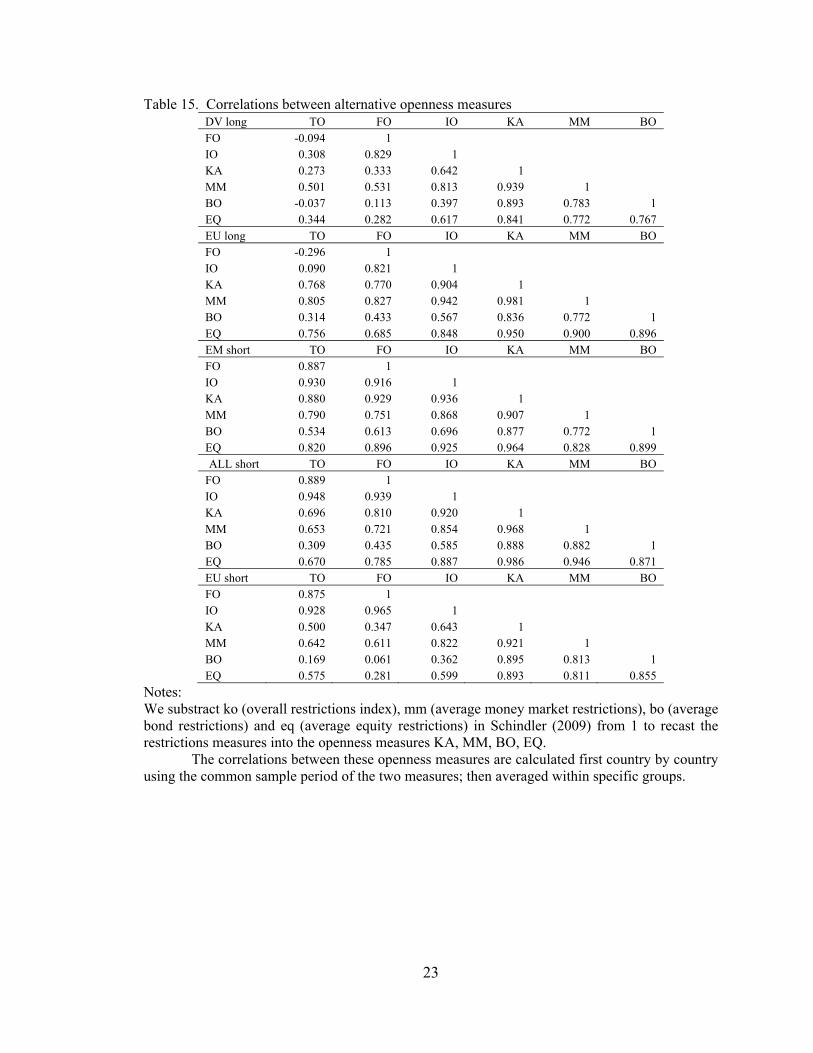
23

Table 15. Correlations between alternative openness measures DV long TO FO IO KA MM BO FO -0.094 1 IO 0.308 0.829 1 KA 0.273 0.333 0.642 1 MM 0.501 0.531 0.813 0.939 1 BO -0.037 0.113 0.397 0.893 0.783 1 EQ 0.344 0.282 0.617 0.841 0.772 0.767 EU long TO FO IO KA MM BO FO -0.296 1 IO 0.090 0.821 1 KA 0.768 0.770 0.904 1 MM 0.805 0.827 0.942 0.981 1 BO 0.314 0.433 0.567 0.836 0.772 1 EQ 0.756 0.685 0.848 0.950 0.900 0.896 EM short TO FO IO KA MM BO FO 0.887 1 IO 0.930 0.916 1 KA 0.880 0.929 0.936 1 MM 0.790 0.751 0.868 0.907 1 BO 0.534 0.613 0.696 0.877 0.772 1 EQ 0.820 0.896 0.925 0.964 0.828 0.899 ALL short TO FO IO KA MM BO

FO 0.889 1 IO 0.948 0.939 1 KA 0.696 0.810 0.920 1 MM 0.653 0.721 0.854 0.968 1 BO 0.309 0.435 0.585 0.888 0.882 1 EQ 0.670 0.785 0.887 0.986 0.946 0.871 EU short TO FO IO KA MM BO FO 0.875 1 IO 0.928 0.965 1 KA 0.500 0.347 0.643 1 MM 0.642 0.611 0.822 0.921 1 BO 0.169 0.061 0.362 0.895 0.813 1 EQ 0.575 0.281 0.599 0.893 0.811 0.855

Notes: We substract ko (overall restrictions index), mm (average money market restrictions), bo (average bond restrictions) and eq (average equity restrictions) in Schindler (2009) from 1 to recast the restrictions measures into the openness measures KA, MM, BO, EQ.

The correlations between these openness measures are calculated first country by country using the common sample period of the two measures; then averaged within specific groups.

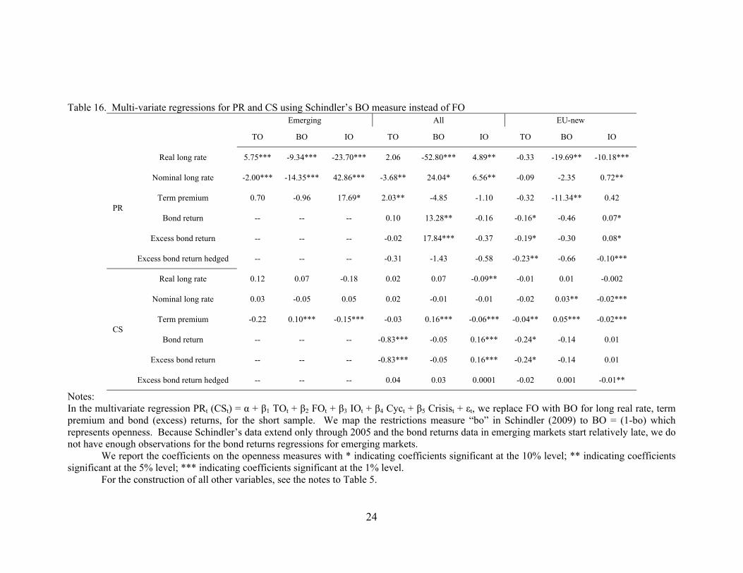
24

Table 16. Multi-variate regressions for PR and CS using Schindler’s BO measure instead of FO Emerging All EU-new

TO BO IO TO BO IO TO BO IO

PR

Real long rate 5.75*** -9.34*** -23.70*** 2.06 -52.80*** 4.89** -0.33 -19.69** -10.18***

Nominal long rate -2.00*** -14.35*** 42.86*** -3.68** 24.04* 6.56** -0.09 -2.35 0.72**

Term premium 0.70 -0.96 17.69* 2.03** -4.85 -1.10 -0.32 -11.34** 0.42

Bond return -- -- -- 0.10 13.28** -0.16 -0.16* -0.46 0.07*

Excess bond return -- -- -- -0.02 17.84*** -0.37 -0.19* -0.30 0.08*

Excess bond return hedged -- -- -- -0.31 -1.43 -0.58 -0.23** -0.66 -0.10***

CS

Real long rate 0.12 0.07 -0.18 0.02 0.07 -0.09** -0.01 0.01 -0.002

Nominal long rate 0.03 -0.05 0.05 0.02 -0.01 -0.01 -0.02 0.03** -0.02***

Term premium -0.22 0.10*** -0.15*** -0.03 0.16*** -0.06*** -0.04** 0.05*** -0.02***

Bond return -- -- -- -0.83*** -0.05 0.16*** -0.24* -0.14 0.01

Excess bond return -- -- -- -0.83*** -0.05 0.16*** -0.24* -0.14 0.01

Excess bond return hedged -- -- -- 0.04 0.03 0.0001 -0.02 0.001 -0.01**

Notes: In the multivariate regression PRt (CSt) = α + β1 TOt + β2 FOt + β3 IOt + β4 Cyct + β5 Crisist + εt, we replace FO with BO for long real rate, term premium and bond (excess) returns, for the short sample. We map the restrictions measure “bo” in Schindler (2009) to BO = (1-bo) which represents openness. Because Schindler’s data extend only through 2005 and the bond returns data in emerging markets start relatively late, we do not have enough observations for the bond returns regressions for emerging markets.

We report the coefficients on the openness measures with * indicating coefficients significant at the 10% level; ** indicating coefficients significant at the 5% level; *** indicating coefficients significant at the 1% level.

For the construction of all other variables, see the notes to Table 5.

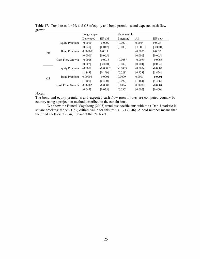
25

Table 17. Trend tests for PR and CS of equity and bond premiums and expected cash flow growth

Long sample Short sample Developed EU-old Emerging All EU-new

PR

Equity Premium -0.0010 -0.0009 -0.0021 0.0034 0.0028

[0.047] [0.042] [0.003] [<.0001] [<.0001]

Bond Premium 0.000003 0.0011 -0.0005 0.0033

[0.0001] [0.065] [0.001] [0.065]

Cash Flow Growth -0.0028 -0.0033 -0.0087 -0.0079 -0.0063

[0.002] [<.0001] [0.089] [0.004] [0.004]

CS

Equity Premium -0.0001 -0.00002 -0.0003 -0.0004 -0.0002

[1.843] [0.199] [0.528] [0.923] [1.454]

Bond Premium 0.00004 -0.0001 0.0009 0.0001 -0.0001

[1.105] [0.400] [0.092] [1.464] [4.486]

Cash Flow Growth 0.00002 -0.0002 0.0006 0.00001 -0.0004

[0.045] [0.075] [0.035] [0.002] [0.460]

Notes: The bond and equity premiums and expected cash flow growth rates are computed country-by-country using a projection method described in the conclusions.

We show the Bunzel-Vogelsang (2005) trend test coefficients with the t-Dan-J statistic in square brackets; the 5% (1%) critical value for this test is 1.71 (2.46). A bold number means that the trend coefficient is significant at the 5% level.

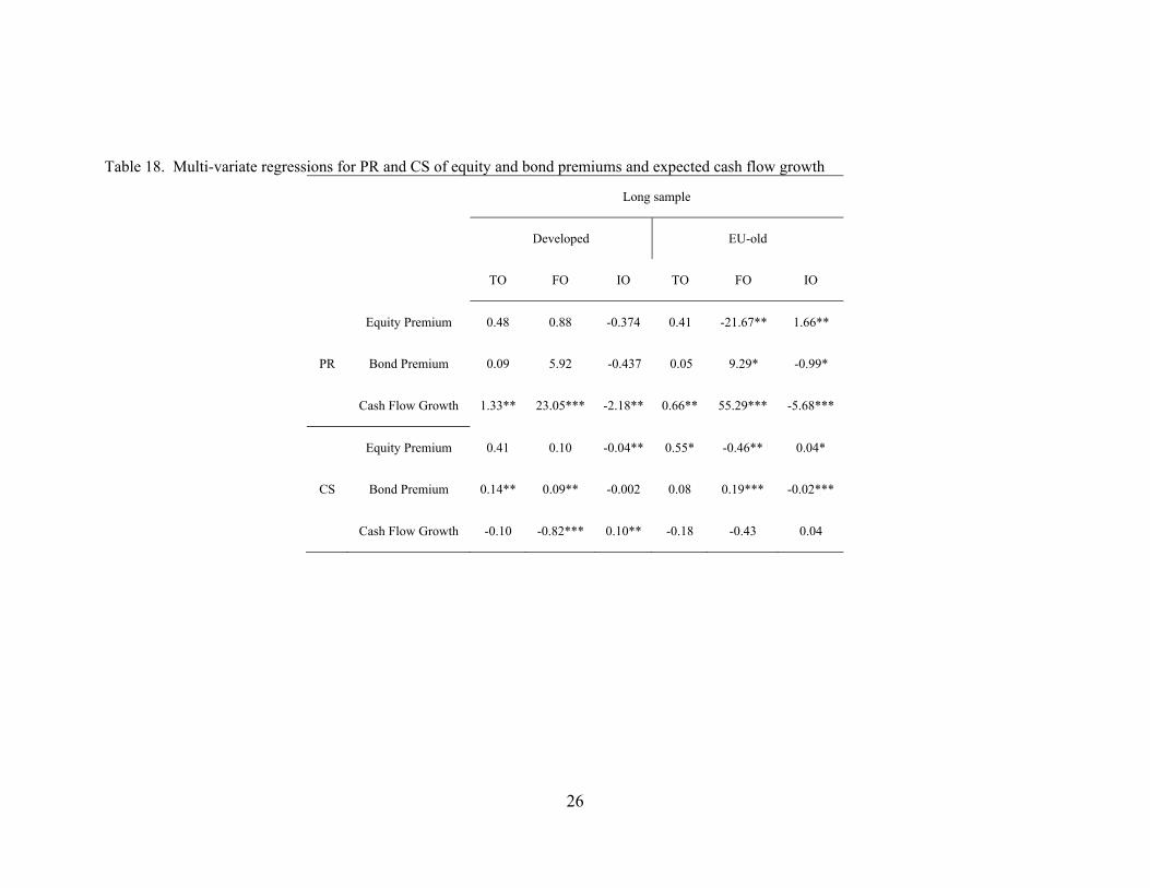
26

Table 18. Multi-variate regressions for PR and CS of equity and bond premiums and expected cash flow growth

Long sample

Developed EU-old

TO FO IO TO FO IO

Equity Premium 0.48 0.88 -0.374 0.41 -21.67** 1.66**

PR Bond Premium 0.09 5.92 -0.437 0.05 9.29* -0.99*

Cash Flow Growth 1.33** 23.05*** -2.18** 0.66** 55.29*** -5.68***

Equity Premium 0.41 0.10 -0.04** 0.55* -0.46** 0.04*

CS Bond Premium 0.14** 0.09** -0.002 0.08 0.19*** -0.02***

Cash Flow Growth -0.10 -0.82*** 0.10** -0.18 -0.43 0.04

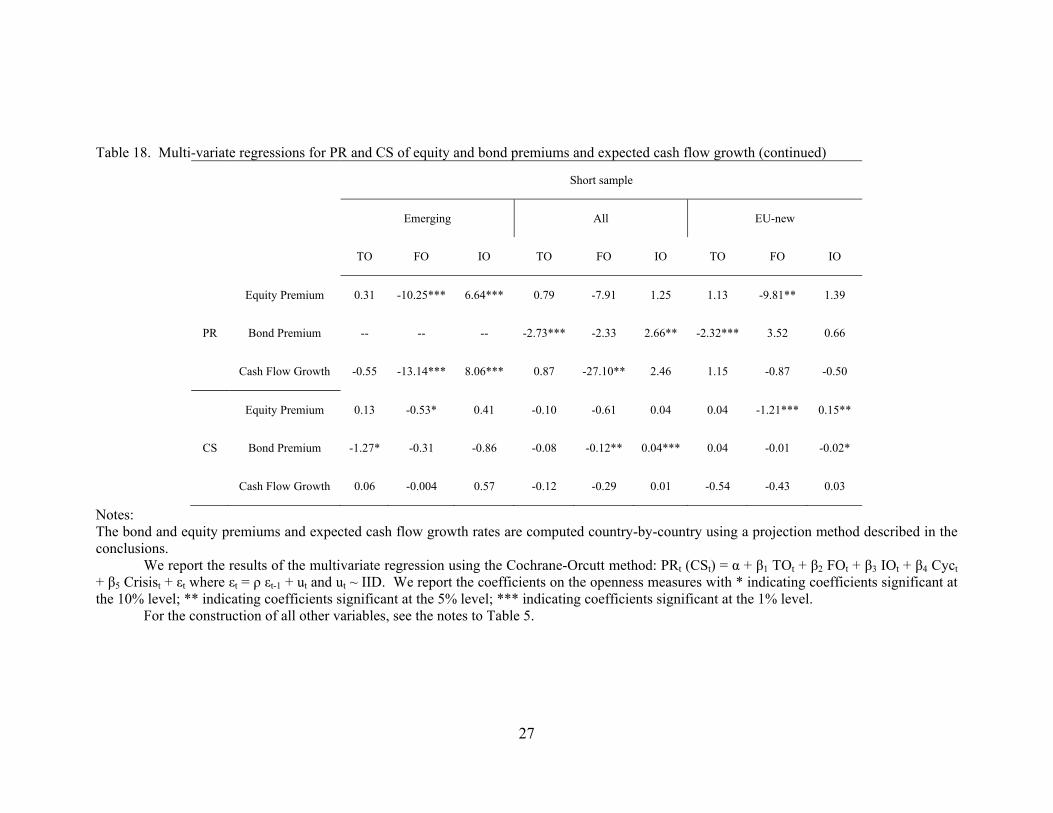
27

Table 18. Multi-variate regressions for PR and CS of equity and bond premiums and expected cash flow growth (continued)

Short sample

Emerging All EU-new

TO FO IO TO FO IO TO FO IO

Equity Premium 0.31 -10.25*** 6.64*** 0.79 -7.91 1.25 1.13 -9.81** 1.39

PR Bond Premium -- -- -- -2.73*** -2.33 2.66** -2.32*** 3.52 0.66

Cash Flow Growth -0.55 -13.14*** 8.06*** 0.87 -27.10** 2.46 1.15 -0.87 -0.50

Equity Premium 0.13 -0.53* 0.41 -0.10 -0.61 0.04 0.04 -1.21*** 0.15**

CS Bond Premium -1.27* -0.31 -0.86 -0.08 -0.12** 0.04*** 0.04 -0.01 -0.02*

Cash Flow Growth 0.06 -0.004 0.57 -0.12 -0.29 0.01 -0.54 -0.43 0.03

Notes: The bond and equity premiums and expected cash flow growth rates are computed country-by-country using a projection method described in the conclusions.

We report the results of the multivariate regression using the Cochrane-Orcutt method: PRt (CSt) = α + β1 TOt + β2 FOt + β3 IOt + β4 Cyct + β5 Crisist + εt where εt = ρ εt-1 + ut and ut ~ IID. We report the coefficients on the openness measures with * indicating coefficients significant at the 10% level; ** indicating coefficients significant at the 5% level; *** indicating coefficients significant at the 1% level.

For the construction of all other variables, see the notes to Table 5.

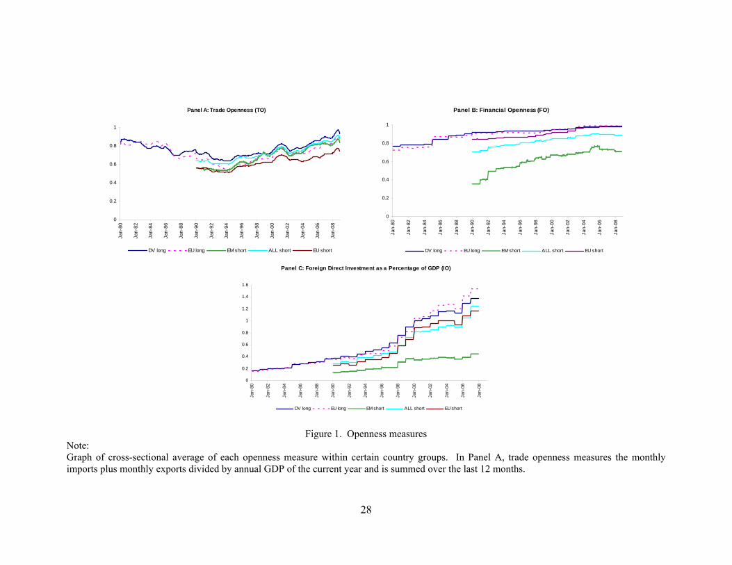
28

Figure 1. Openness measures Note: Graph of cross-sectional average of each openness measure within certain country groups. In Panel A, trade openness measures the monthly imports plus monthly exports divided by annual GDP of the current year and is summed over the last 12 months.

Panel A: Trade Openness (TO)

0

0.2

0.4

0.6

0.8

1Ja

n-80

Jan-

82

Jan-

84

Jan-

86

Jan-

88

Jan-

90

Jan-

92

Jan-

94

Jan-

96

Jan-

98

Jan-

00

Jan-

02

Jan-

04

Jan-

06

Jan-

08

DV long EU long EM short ALL short EU short

Panel B: Financial Openness (FO)

0

0.2

0.4

0.6

0.8

1

Jan-

80

Jan-

82

Jan-

84

Jan-

86

Jan-

88

Jan-

90

Jan-

92

Jan-

94

Jan-

96

Jan-

98

Jan-

00

Jan-

02

Jan-

04

Jan-

06

Jan-

08

DV long EU long EM short ALL short EU short

Panel C: Foreign Direct Investment as a Percentage of GDP (IO)

0

0.2

0.4

0.6

0.8

1

1.2

1.4

1.6

Jan-

80

Jan-

82

Jan-

84

Jan-

86

Jan-

88

Jan-

90

Jan-

92

Jan-

94

Jan-

96

Jan-

98

Jan-

00

Jan-

02

Jan-

04

Jan-

06

Jan-

08

DV long EU long EM short ALL short EU short

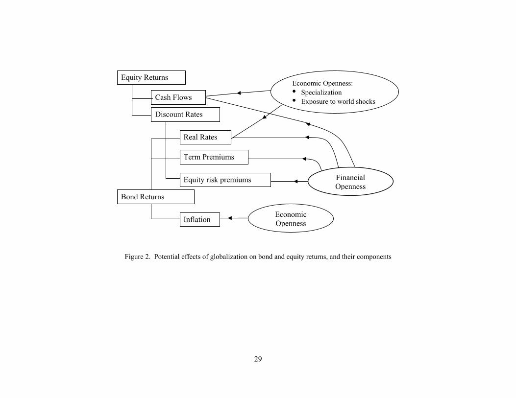
29

Figure 2. Potential effects of globalization on bond and equity returns, and their components

Equity Returns

Cash Flows

Discount Rates

Real Rates

Term Premiums

Equity risk premiums

Bond Returns

Economic Openness: • Specialization • Exposure to world shocks

Inflation Economic Openness

Financial Openness

30

Figure 3-a. Portfolio variance ratios of interest rate variables

1980 1985 1990 1995 2000 20050

0.5

1PR: Real Short Rates

PR_DEV_L

PR_EU_L

PR_EM_SPR_ALL_S

PR_EU_S

1980 1985 1990 1995 2000 20050

0.5

1PR: Real Long Rates

PR_DEV_L

PR_EU_L

PR_EM_SPR_ALL_S

PR_EU_S

1980 1985 1990 1995 2000 20050

0.5

1PR: Inflation

PR_DEV_L

PR_EU_L

PR_EM_SPR_ALL_S

PR_EU_S

1980 1985 1990 1995 2000 20050

0.5

1PR: Nominal Short Rates

PR_DEV_L

PR_EU_L

PR_EM_SPR_ALL_S

PR_EU_S

1980 1985 1990 1995 2000 20050

0.5

1PR: Nominal long Rates

PR_DEV_L

PR_EU_L

PR_EM_SPR_ALL_S

PR_EU_S

1980 1985 1990 1995 2000 20050

0.5

1PR: Term Premium

PR_DEV_L

PR_EU_L

PR_EM_SPR_ALL_S

PR_EU_S

31

Figure 3-b. Portfolio variance ratios of return variables

1980 1985 1990 1995 2000 20050

0.5

1PR: Bond Return

PR_DEV_L

PR_EU_L

PR_EM_SPR_ALL_S

PR_EU_S

1980 1985 1990 1995 2000 20050

0.5

1PR: Excess Bond Return

PR_DEV_L

PR_EU_L

PR_EM_SPR_ALL_S

PR_EU_S

1980 1985 1990 1995 2000 20050

0.5

1PR: Excess Bond Return Hedged

PR_DEV_L

PR_EU_L

PR_EM_SPR_ALL_S

PR_EU_S

1980 1985 1990 1995 2000 20050

0.5

1PR: Equity Return

PR_DEV_L

PR_EU_L

PR_EM_SPR_ALL_S

PR_EU_S

1980 1985 1990 1995 2000 20050

0.5

1PR: Excess Equity Return

PR_DEV_L

PR_EU_L

PR_EM_SPR_ALL_S

PR_EU_S

1980 1985 1990 1995 2000 20050

0.5

1PR: Excess Equity Return Hedged

PR_DEV_L

PR_EU_L

PR_EM_SPR_ALL_S

PR_EU_S

32

Figure 3-c. Portfolio variance ratios of equity valuation variables Note: Each panel shows the times series of a variable for 5 samples, with “_DEV_L” indicating developed long sample; “_EU_L” indicating EU long sample; “_EM_S” indicating emerging short sample; “_ALL_S” indicating all countries short sample; and “_EU_S” indicating EU short sample.

1980 1985 1990 1995 2000 20050

0.5

1PR: Cash Flow Growth

PR_DEV_L

PR_EU_L

PR_EM_SPR_ALL_S

PR_EU_S

1980 1985 1990 1995 2000 20050

0.5

1PR: Log(PE)

PR_DEV_L

PR_EU_L

PR_EM_SPR_ALL_S

PR_EU_S

33

Figure 4-a. Variance ratios of interest rate variables (xglob,t = xUS,t)

1980 1985 1990 1995 2000 20050

0.2

0.4

0.6

0.8

1VR: Real Short Rates

VR_DEV_L

VR_EU_L

VR_EM_SVR_ALL_S

VR_EU_S

1980 1985 1990 1995 2000 20050

0.2

0.4

0.6

0.8

1VR: Real Long Rates

VR_DEV_L

VR_EU_L

VR_EM_SVR_ALL_S

VR_EU_S

1980 1985 1990 1995 2000 20050

0.2

0.4

0.6

0.8

1VR: Inflation

VR_DEV_L

VR_EU_L

VR_EM_SVR_ALL_S

VR_EU_S

1980 1985 1990 1995 2000 20050

0.2

0.4

0.6

0.8

1VR: Nominal Short Rates

VR_DEV_L

VR_EU_L

VR_EM_SVR_ALL_S

VR_EU_S

1980 1985 1990 1995 2000 20050

0.2

0.4

0.6

0.8

1VR: Nominal long Rates

VR_DEV_L

VR_EU_L

VR_EM_SVR_ALL_S

VR_EU_S

1980 1985 1990 1995 2000 20050

0.5

1VR: Term Premium

VR_DEV_L

VR_EU_L

VR_EM_SVR_ALL_S

VR_EU_S

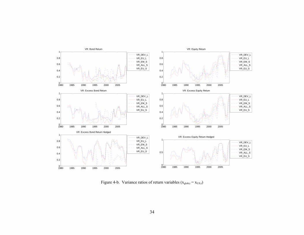
34

Figure 4-b. Variance ratios of return variables (xglob,t = xUS,t)

1980 1985 1990 1995 2000 20050

0.2

0.4

0.6

0.8

1VR: Bond Return

VR_DEV_L

VR_EU_L

VR_EM_SVR_ALL_S

VR_EU_S

1980 1985 1990 1995 2000 20050

0.2

0.4

0.6

0.8

1VR: Excess Bond Return

VR_DEV_L

VR_EU_L

VR_EM_SVR_ALL_S

VR_EU_S

1980 1985 1990 1995 2000 20050

0.2

0.4

0.6

0.8

1VR: Excess Bond Return Hedged

VR_DEV_L

VR_EU_L

VR_EM_SVR_ALL_S

VR_EU_S

1980 1985 1990 1995 2000 20050

0.2

0.4

0.6

0.8

1VR: Equity Return

VR_DEV_L

VR_EU_L

VR_EM_SVR_ALL_S

VR_EU_S

1980 1985 1990 1995 2000 20050

0.2

0.4

0.6

0.8

1VR: Excess Equity Return

VR_DEV_L

VR_EU_L

VR_EM_SVR_ALL_S

VR_EU_S

1980 1985 1990 1995 2000 20050

0.5

1VR: Excess Equity Return Hedged

VR_DEV_L

VR_EU_L

VR_EM_SVR_ALL_S

VR_EU_S

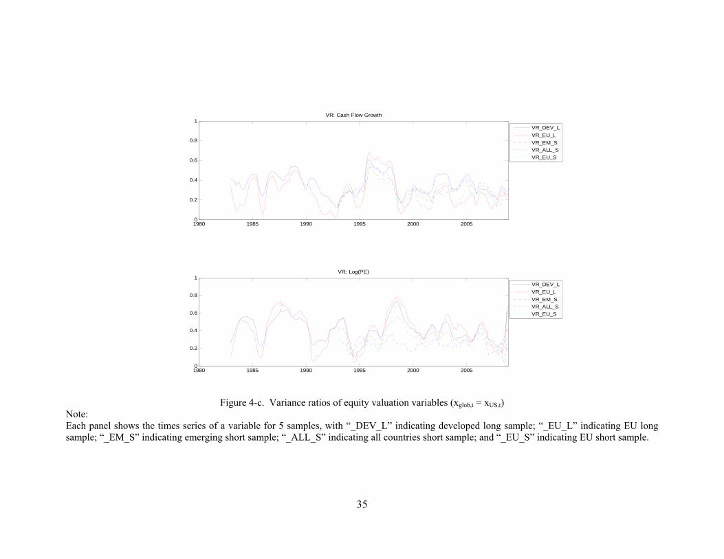
35

Figure 4-c. Variance ratios of equity valuation variables (xglob,t = xUS,t)

Note: Each panel shows the times series of a variable for 5 samples, with “_DEV_L” indicating developed long sample; “_EU_L” indicating EU long sample; “_EM_S” indicating emerging short sample; “_ALL_S” indicating all countries short sample; and “_EU_S” indicating EU short sample.

1980 1985 1990 1995 2000 20050

0.2

0.4

0.6

0.8

1VR: Cash Flow Growth

VR_DEV_L

VR_EU_L

VR_EM_SVR_ALL_S

VR_EU_S

1980 1985 1990 1995 2000 20050

0.2

0.4

0.6

0.8

1VR: Log(PE)

VR_DEV_L

VR_EU_L

VR_EM_SVR_ALL_S

VR_EU_S

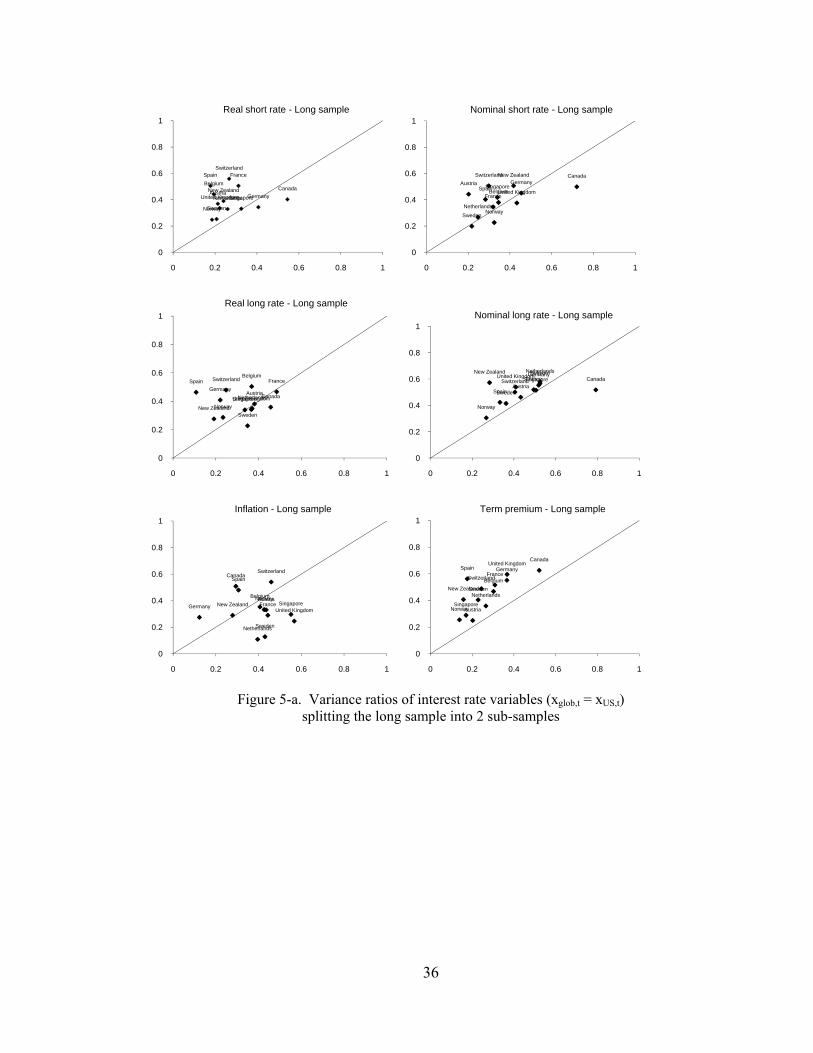
36

Figure 5-a. Variance ratios of interest rate variables (xglob,t = xUS,t) splitting the long sample into 2 sub-samples

Austria

Belgium Canada

France

Germany Netherlands

New Zealand

Norway

Singapore

Spain

Sweden

Switzerland

United Kingdom

0

0.2

0.4

0.6

0.8

1

0 0.2 0.4 0.6 0.8 1

Real short rate - Long sample

Austria

Belgium

Canada

France

Germany

Netherlands

New Zealand

Norway

Singapore Spain

Sweden

Switzerland

United Kingdom

0

0.2

0.4

0.6

0.8

1

0 0.2 0.4 0.6 0.8 1

Nominal short rate - Long sample

Austria

Belgium

Canada

France

Germany

Netherlands

New Zealand Norway

Singapore

Spain

Sweden

Switzerland

United Kingdom

0

0.2

0.4

0.6

0.8

1

0 0.2 0.4 0.6 0.8 1

Real long rate - Long sample

Austria

Belgium Canada France

Germany Netherlands New Zealand

Norway

Singapore

Spain Sweden

Switzerland United Kingdom

0

0.2

0.4

0.6

0.8

1

0 0.2 0.4 0.6 0.8 1

Nominal long rate - Long sample

Austria Belgium

Canada

France Germany

Netherlands

New Zealand Norway

Singapore

Spain

Sweden

Switzerland

United Kingdom

0

0.2

0.4

0.6

0.8

1

0 0.2 0.4 0.6 0.8 1

Inflation - Long sample

Austria

Belgium

Canada

France Germany

Netherlands New Zealand

Norway Singapore

Spain

Sweden

Switzerland

United Kingdom

0

0.2

0.4

0.6

0.8

1

0 0.2 0.4 0.6 0.8 1

Term premium - Long sample

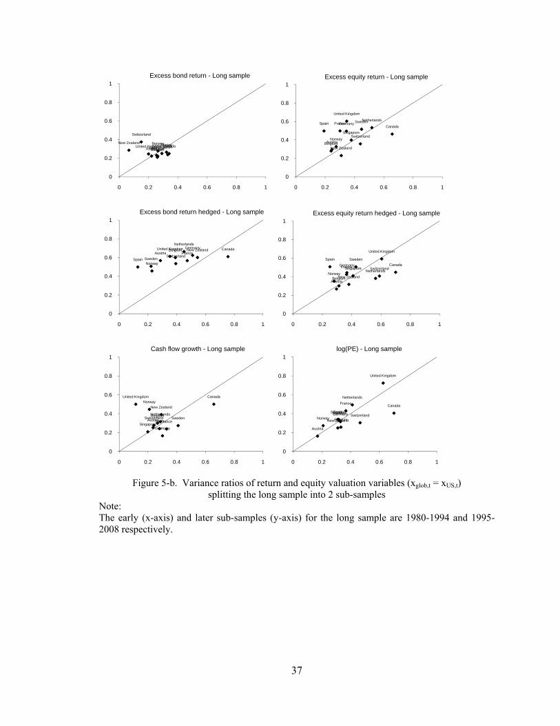
37

Figure 5-b. Variance ratios of return and equity valuation variables (xglob,t = xUS,t) splitting the long sample into 2 sub-samples

Note: The early (x-axis) and later sub-samples (y-axis) for the long sample are 1980-1994 and 1995-2008 respectively.

Austria Belgium Canada France

Germany Netherlands New Zealand Norway

Spain Sweden

Switzerland

United Kingdom

0

0.2

0.4

0.6

0.8

1

0 0.2 0.4 0.6 0.8 1

Excess bond return - Long sample

Austria Belgium

Canada France Germany

Netherlands

New Zealand

Norway

Singapore

Spain Sweden

Switzerland

United Kingdom

0

0.2

0.4

0.6

0.8

1

0 0.2 0.4 0.6 0.8 1

Excess equity return - Long sample

Austria Belgium Canada

France

Germany Netherlands

New Zealand

Norway Spain Sweden

Switzerland

United Kingdom

0

0.2

0.4

0.6

0.8

1

0 0.2 0.4 0.6 0.8 1

Excess bond return hedged - Long sample

Austria Belgium

Canada France Germany

Netherlands

New Zealand Norway

Singapore

Spain Sweden

Switzerland

United Kingdom

0

0.2

0.4

0.6

0.8

1

0 0.2 0.4 0.6 0.8 1

Excess equity return hedged - Long sample

Austria Belgium

Canada

France

Germany

Netherlands

New Zealand

Norway

Singapore Spain

Sweden Switzerland

United Kingdom

0

0.2

0.4

0.6

0.8

1

0 0.2 0.4 0.6 0.8 1

Cash flow growth - Long sample

Austria

Belgium

Canada France

Germany

Netherlands

New Zealand Norway

Singapore Spain Sweden Switzerland

United Kingdom

0

0.2

0.4

0.6

0.8

1

0 0.2 0.4 0.6 0.8 1

log(PE) - Long sample

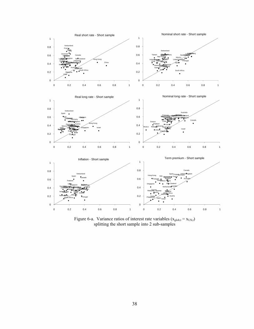
38

Figure 6-a. Variance ratios of interest rate variables (xglob,t = xUS,t) splitting the short sample into 2 sub-samples

Australia

Austria

Belgium Canada

Chile

China

Denmark

Finland

France

Germany

Greece Hong Kong

Indonesia

Ireland

Israel

Italy

Japan Korea

Malaysia

Mexico Netherlands

New Zealand

Norway Philippines

Portugal

Singapore

South Africa

Spain

Sweden

Switzerland

Taiwan Thailand United Kingdom

0

0.2

0.4

0.6

0.8

1

0 0.2 0.4 0.6 0.8 1

Real short rate - Short sample

Australia Austria

Belgium

Canada

Chile

China

Denmark Finland France

Germany

Greece

Hong Kong

Indonesia

Ireland

Israel

Italy

Japan

Korea

Malaysia

Mexico

Netherlands

New Zealand

Norway Philippines

Portugal

Singapore

South Africa

Spain

Sweden

Switzerland

Taiwan Thailand

United Kingdom

0

0.2

0.4

0.6

0.8

1

0 0.2 0.4 0.6 0.8 1

Nominal short rate - Short sample

Australia

Austria

Belgium Canada

Chile China

Denmark Finland

France Germany

Greece

Hong Kong

Indonesia

Ireland Israel

Italy

Japan

Korea

Malaysia

Mexico Netherlands New Zealand Norway Philippines

Portugal

Singapore

South Africa

Spain

Sweden

Switzerland

Taiwan

Thailand United Kingdom

0

0.2

0.4

0.6

0.8

1

0 0.2 0.4 0.6 0.8 1

Real long rate - Short sample

Australia

Austria

Belgium

Canada Chile

China

Denmark Finland France Germany

Greece Hong Kong

Indonesia

Ireland

Israel

Italy Japan

Korea Malaysia Mexico

Netherlands New Zealand

Norway

Philippines

Portugal

Singapore

South Africa

Spain

Sweden

Switzerland

Taiwan

Thailand

United Kingdom

0

0.2

0.4

0.6

0.8

1

0 0.2 0.4 0.6 0.8 1

Nominal long rate - Short sample

Australia Austria

Belgium

Canada

Chile

China

Denmark Finland France

Germany

Greece

Hong Kong

Indonesia

Ireland

IsraelItaly

Japan Korea

Malaysia Mexico

Netherlands

New Zealand

Norway Philippines

Portugal

Singapore

South Africa

Spain

Sweden

Switzerland

Taiwan

Thailand

United Kingdom

0

0.2

0.4

0.6

0.8

1

0 0.2 0.4 0.6 0.8 1

Inflation - Short sample

Australia

Austria

Belgium

Canada

Chile

China

Denmark

Finland France

Germany

Greece

Hong Kong

Indonesia

Ireland

Israel

Italy

Japan Korea

Malaysia Mexico

Netherlands

New Zealand

Norway

Philippines

Portugal

Singapore

South Africa

Spain

Sweden

Switzerland

Taiwan Thailand

United Kingdom

0

0.2

0.4

0.6

0.8

1

0 0.2 0.4 0.6 0.8 1

Term premium - Short sample

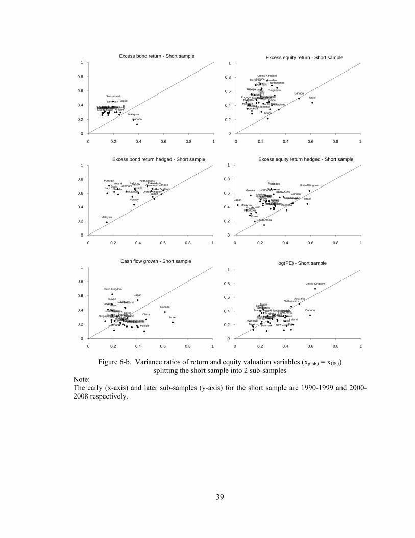
39

Figure 6-b. Variance ratios of return and equity valuation variables (xglob,t = xUS,t) splitting the short sample into 2 sub-samples

Note: The early (x-axis) and later sub-samples (y-axis) for the short sample are 1990-1999 and 2000-2008 respectively.

Australia Austria Belgium

Canada

Denmark

Finland France Germany Ireland Italy

Japan

Malaysia

Netherlands New Zealand Norway Portugal Spain Sweden

Switzerland

United Kingdom

0

0.2

0.4

0.6

0.8

1

0 0.2 0.4 0.6 0.8 1

Excess bond return - Short sample

Australia

Austria Belgium

Canada Chile

China

Denmark

Finland

France Germany

Greece Hong Kong

Indonesia

Ireland Israel

Italy

Japan

Korea

Malaysia

Mexico

Netherlands

New Zealand

Norway

Philippines

Portugal

Singapore

South Africa

Spain Sweden

Switzerland Taiwan

Thailand

United Kingdom

0

0.2

0.4

0.6

0.8

1

0 0.2 0.4 0.6 0.8 1

Excess equity return - Short sample

Australia

Austria

Belgium Canada Denmark Finland France Germany

Ireland

Italy

Japan

Malaysia

Netherlands

New Zealand

Norway

Portugal

Spain Sweden

Switzerland United Kingdom

0

0.2

0.4

0.6

0.8

1

0 0.2 0.4 0.6 0.8 1

Excess bond return hedged - Short sample

Australia Austria

Belgium

Canada

Chile China

Denmark Finland

France Germany Greece Hong Kong

Indonesia

Ireland

IsraelItaly

Japan

Korea

Malaysia

Mexico

Netherlands

New Zealand

Norway

Philippines

Portugal

Singapore

South Africa

Spain Sweden

Switzerland Taiwan

Thailand

United Kingdom

0

0.2

0.4

0.6

0.8

1

0 0.2 0.4 0.6 0.8 1

Excess equity return hedged - Short sample

Australia Austria

Belgium

Canada

Chile China

Denmark

Finland France

Germany

Greece Hong Kong Indonesia

Ireland Israel

Italy

Japan

Korea Malaysia

Mexico

Netherlands

New Zealand Norway

Philippines Portugal

Singapore South Africa

Spain

Sweden Switzerland

Taiwan

Thailand

United Kingdom

0

0.2

0.4

0.6

0.8

1

0 0.2 0.4 0.6 0.8 1

Cash flow growth - Short sample

Australia

Austria

Belgium

Canada

Chile

China

Denmark

Finland France

Germany

Greece Hong Kong

Indonesia Ireland Israel

Italy

Japan

Korea

Malaysia

Mexico

Netherlands

New Zealand

Norway Philippines Portugal

Singapore

South Africa Spain

Sweden

Switzerland

Taiwan

Thailand

United Kingdom

0

0.2

0.4

0.6

0.8

1

0 0.2 0.4 0.6 0.8 1

log(PE) - Short sample

40

Figure 7: World interest rate with “standard error” bounds for DV and EU sub-samples Note: We show the Cochrane-Orcutt estimates of (µ+gt) in regressions for different country groups: xi,t

= µ + gt + αi + εi,t and the upper and lower bound calculated as

∑ , ,

-0.08

-0.04

0

0.04

0.08

0.12

1980 1985 1990 1995 2000 2005

Real short rate - DV long sample

-0.08

-0.04

0

0.04

0.08

0.12

1980 1985 1990 1995 2000 2005

Real long rate - DV long sample

-0.08

-0.04

0

0.04

0.08

0.12

1980 1985 1990 1995 2000 2005

Real long rate - EU long & short sample

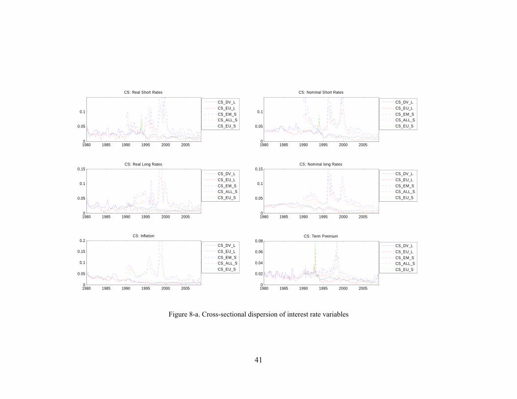
41

Figure 8-a. Cross-sectional dispersion of interest rate variables

1980 1985 1990 1995 2000 20050

0.05

0.1

CS: Real Short Rates

CS_DV_L

CS_EU_L

CS_EM_SCS_ALL_S

CS_EU_S

1980 1985 1990 1995 2000 20050

0.05

0.1

0.15CS: Real Long Rates

CS_DV_L

CS_EU_L

CS_EM_SCS_ALL_S

CS_EU_S

1980 1985 1990 1995 2000 20050

0.05

0.1

0.15

0.2CS: Inflation

CS_DV_L

CS_EU_L

CS_EM_SCS_ALL_S

CS_EU_S

1980 1985 1990 1995 2000 20050

0.05

0.1

CS: Nominal Short Rates

CS_DV_L

CS_EU_L

CS_EM_SCS_ALL_S

CS_EU_S

1980 1985 1990 1995 2000 20050

0.05

0.1

0.15CS: Nominal long Rates

CS_DV_L

CS_EU_L

CS_EM_SCS_ALL_S

CS_EU_S

1980 1985 1990 1995 2000 20050

0.02

0.04

0.06

0.08CS: Term Premium

CS_DV_L

CS_EU_L

CS_EM_SCS_ALL_S

CS_EU_S

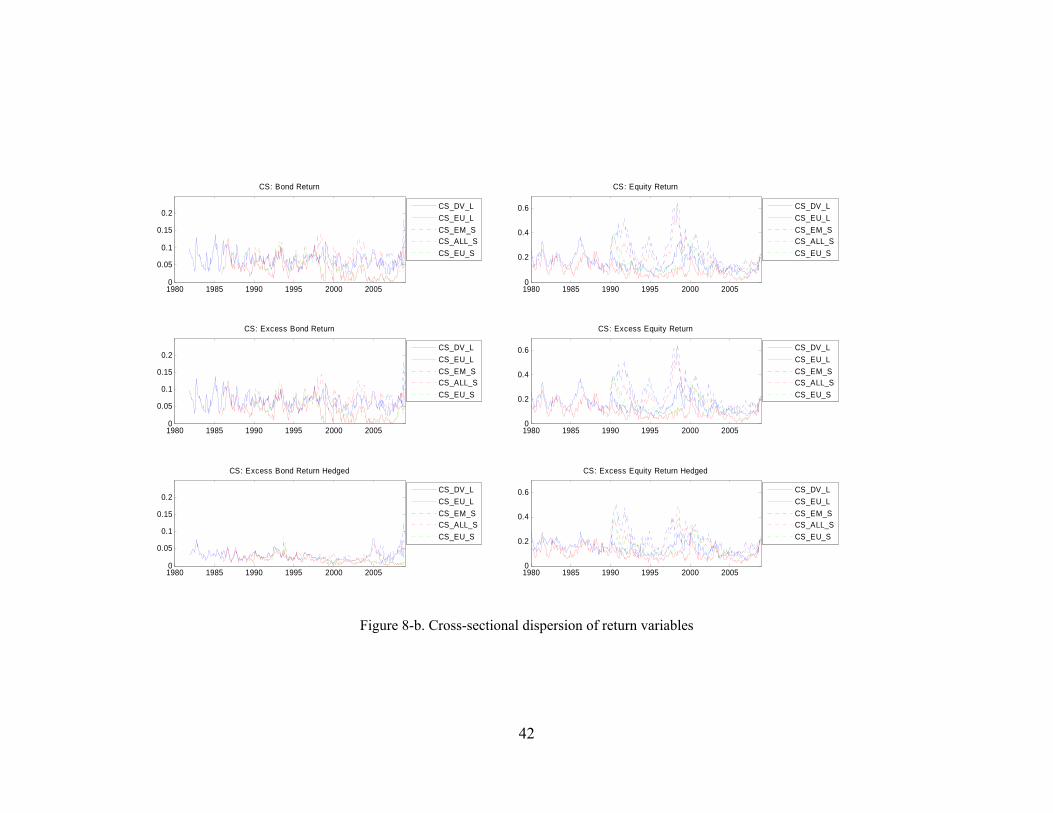
42

Figure 8-b. Cross-sectional dispersion of return variables

1980 1985 1990 1995 2000 20050

0.05

0.1

0.15

0.2

CS: Bond Return

CS_DV_L

CS_EU_L

CS_EM_SCS_ALL_S

CS_EU_S

1980 1985 1990 1995 2000 20050

0.05

0.1

0.15

0.2

CS: Excess Bond Return

CS_DV_L

CS_EU_L

CS_EM_SCS_ALL_S

CS_EU_S

1980 1985 1990 1995 2000 20050

0.05

0.1

0.15

0.2

CS: Excess Bond Return Hedged

CS_DV_L

CS_EU_L

CS_EM_SCS_ALL_S

CS_EU_S

1980 1985 1990 1995 2000 20050

0.2

0.4

0.6

CS: Equity Return

CS_DV_L

CS_EU_L

CS_EM_SCS_ALL_S

CS_EU_S

1980 1985 1990 1995 2000 20050

0.2

0.4

0.6

CS: Excess Equity Return

CS_DV_L

CS_EU_L

CS_EM_SCS_ALL_S

CS_EU_S

1980 1985 1990 1995 2000 20050

0.2

0.4

0.6

CS: Excess Equity Return Hedged

CS_DV_L

CS_EU_L

CS_EM_SCS_ALL_S

CS_EU_S

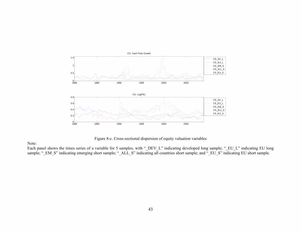
43

Figure 8-c. Cross-sectional dispersion of equity valuation variables Note: Each panel shows the times series of a variable for 5 samples, with “_DEV_L” indicating developed long sample; “_EU_L” indicating EU long sample; “_EM_S” indicating emerging short sample; “_ALL_S” indicating all countries short sample; and “_EU_S” indicating EU short sample.

1980 1985 1990 1995 2000 20050

0.5

1

1.5

CS: Cash Flow Growth

CS_DV_L

CS_EU_L

CS_EM_SCS_ALL_S

CS_EU_S

1980 1985 1990 1995 2000 20050

0.2

0.4

0.6

0.8CS: Log(PE)

CS_DV_L

CS_EU_L

CS_EM_SCS_ALL_S

CS_EU_S

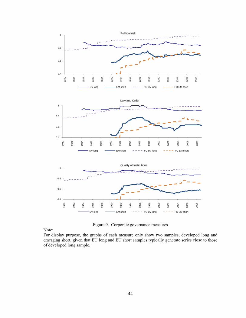
44

Figure 9. Corporate governance measures Note: For display purpose, the graphs of each measure only show two samples, developed long and emerging short, given that EU long and EU short samples typically generate series close to those of developed long sample.

0.4

0.6

0.8

1

19

80

19

82

19

84

19

86

19

88

19

90

19

92

19

94

19

96

19

98

20

00

20

02

20

04

20

06

20

08

Political risk

DV long EM short FO DV long FO EM short

0.4

0.6

0.8

1

19

80

19

82

19

84

19

86

19

88

19

90

19

92

19

94

19

96

19

98

20

00

20

02

20

04

20

06

20

08

Law and Order

DV long EM short FO DV long FO EM short

0.4

0.6

0.8

1

19

80

19

82

19

84

19

86

19

88

19

90

19

92

19

94

19

96

19

98

20

00

20

02

20

04

20

06

20

08

Quality of Institutions

DV long EM short FO DV long FO EM short

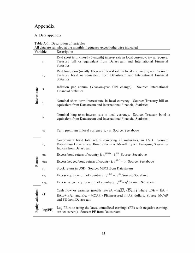
45

Appendix A Data appendix Table A-1. Description of variables All data are sampled at the monthly frequency except otherwise indicated Variable Description

Inte

rest

rat

e

r1 Real short term (mostly 3-month) interest rate in local currency: i1 – π. Source: Treasury bill or equivalent from Datastream and International Financial Statistics

rn Real long term (mostly 10-year) interest rate in local currency: in – π. Source: Treasury bond or equivalent from Datastream and International Financial Statistics

π Inflation per annum (Year-on-year CPI change). Source: International Financial Statistics

i1 Nominal short term interest rate in local currency. Source: Treasury bill or equivalent from Datastream and International Financial Statistics

in Nominal long term interest rate in local currency. Source: Treasury bond orequivalent from Datastream and International Financial Statistics

tp Term premium in local currency: in - i1. Source: See above

Ret

urns

rb Government bond total return (covering all maturities) in USD. Source: Datastream Government Bond indices or Merrill Lynch Emerging Sovereign Indices from Datastream

erb Excess bond return of country j: rbj,USD – i1

US. Source: See above

erhb Excess hedged bond return of country j: rbj,LC – i1

j. Source: See above

rs Stock return in USD. Source: MSCI from Datastream

ers Excess equity return of country j: rsj,USD – i1

US. Source: See above

erhs Excess hedged equity return of country j: rsj,LC – i1

j. Source: See above

Equ

ity

valu

atio

n

cf Cash flow or earnings growth rate where = EAt +

EAt-1 + EAt-2 and EAt = MCAPt / PEt measured in U.S. dollars. Source: MCAP and PE from Datastream

log(PE) Log PE ratio using the latest annualized earnings (PEs with negative earnings are set as zero). Source: PE from Datastream

)/ln( 12 ttt EAEAcf tEA

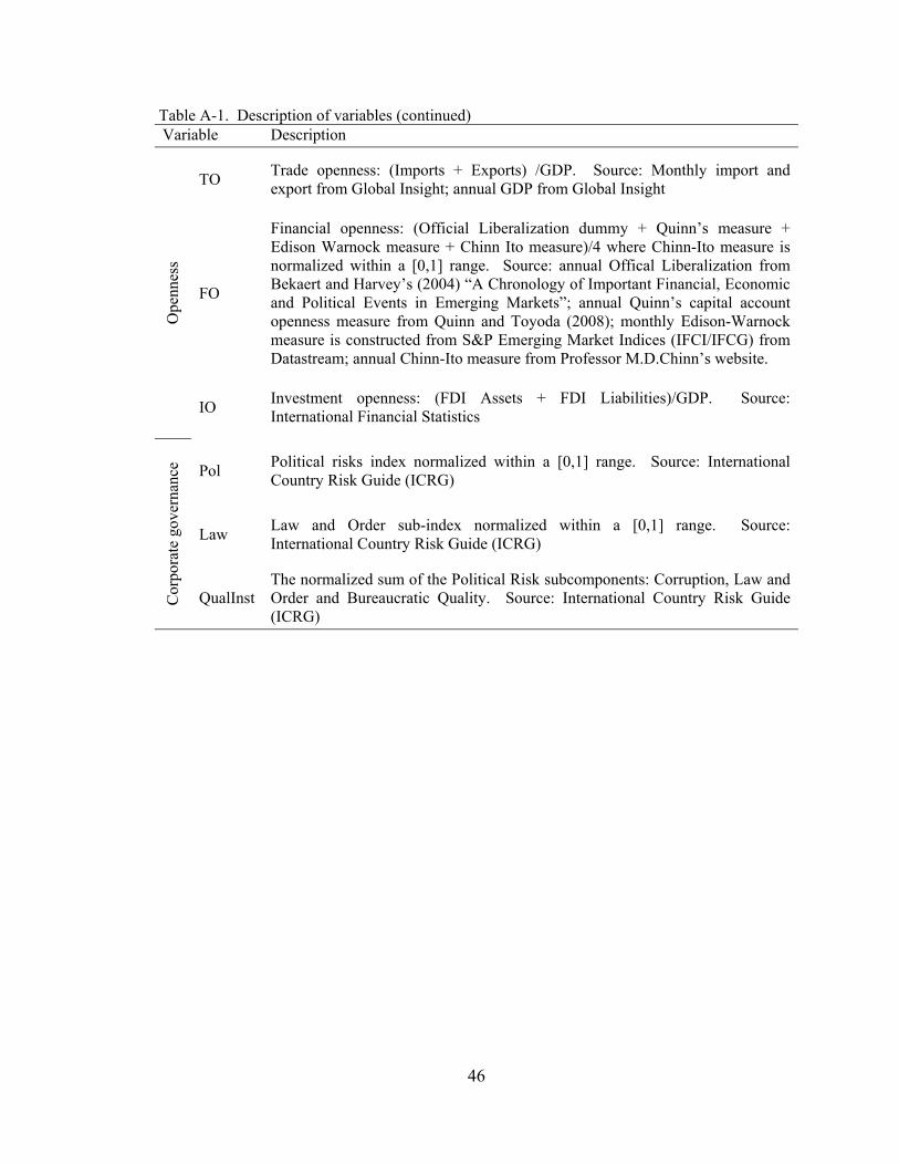
46

Table A-1. Description of variables (continued) Variable Description

Ope

nnes

s TO

Trade openness: (Imports + Exports) /GDP. Source: Monthly import and export from Global Insight; annual GDP from Global Insight

FO

Financial openness: (Official Liberalization dummy + Quinn’s measure + Edison Warnock measure + Chinn Ito measure)/4 where Chinn-Ito measure is normalized within a [0,1] range. Source: annual Offical Liberalization from Bekaert and Harvey’s (2004) “A Chronology of Important Financial, Economic and Political Events in Emerging Markets”; annual Quinn’s capital account openness measure from Quinn and Toyoda (2008); monthly Edison-Warnock measure is constructed from S&P Emerging Market Indices (IFCI/IFCG) from Datastream; annual Chinn-Ito measure from Professor M.D.Chinn’s website.

IO Investment openness: (FDI Assets + FDI Liabilities)/GDP. Source: International Financial Statistics

Cor

pora

te g

over

nanc

e Pol Political risks index normalized within a [0,1] range. Source: International Country Risk Guide (ICRG)

Law Law and Order sub-index normalized within a [0,1] range. Source: International Country Risk Guide (ICRG)

QualInst The normalized sum of the Political Risk subcomponents: Corruption, Law and Order and Bureaucratic Quality. Source: International Country Risk Guide (ICRG)

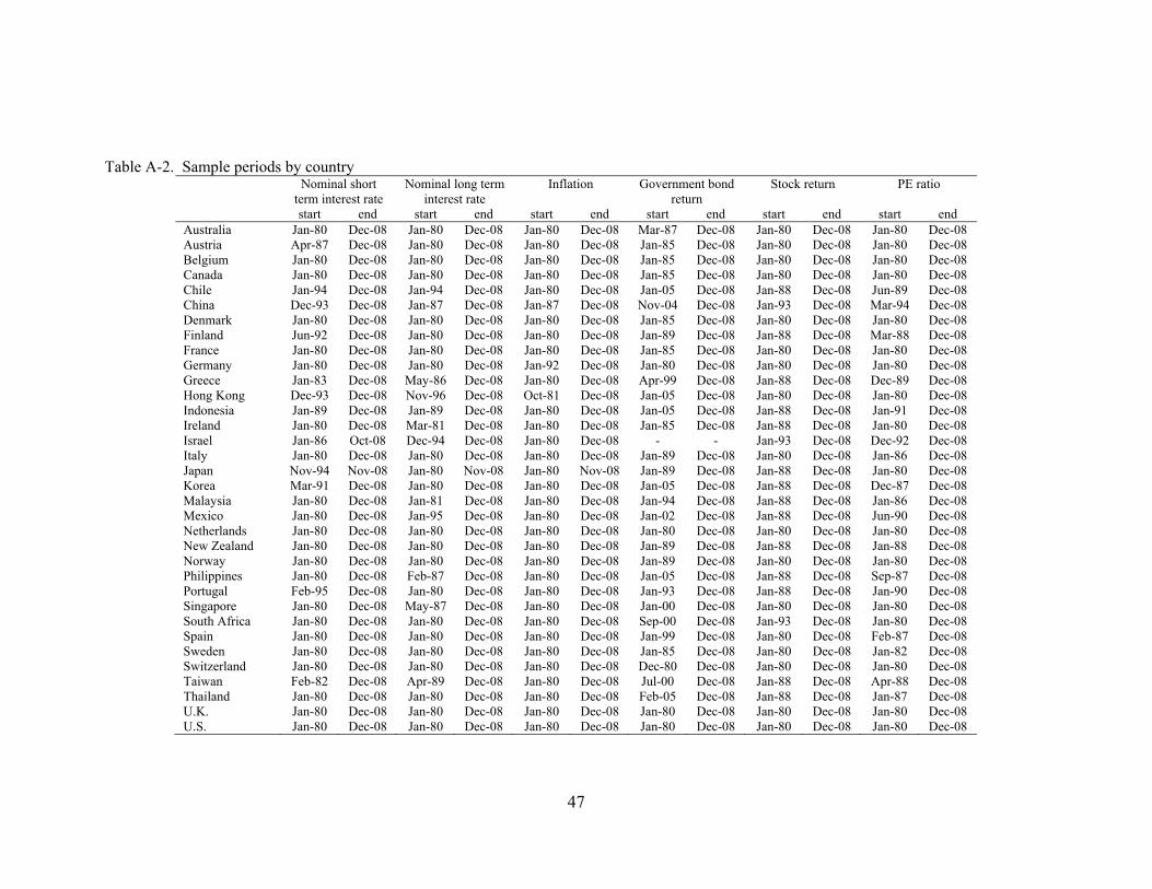
47

Table A-2. Sample periods by country Nominal short

term interest rate Nominal long term

interest rate Inflation Government bond

return Stock return PE ratio

start end start end start end start end start end start end Australia Jan-80 Dec-08 Jan-80 Dec-08 Jan-80 Dec-08 Mar-87 Dec-08 Jan-80 Dec-08 Jan-80 Dec-08 Austria Apr-87 Dec-08 Jan-80 Dec-08 Jan-80 Dec-08 Jan-85 Dec-08 Jan-80 Dec-08 Jan-80 Dec-08 Belgium Jan-80 Dec-08 Jan-80 Dec-08 Jan-80 Dec-08 Jan-85 Dec-08 Jan-80 Dec-08 Jan-80 Dec-08 Canada Jan-80 Dec-08 Jan-80 Dec-08 Jan-80 Dec-08 Jan-85 Dec-08 Jan-80 Dec-08 Jan-80 Dec-08 Chile Jan-94 Dec-08 Jan-94 Dec-08 Jan-80 Dec-08 Jan-05 Dec-08 Jan-88 Dec-08 Jun-89 Dec-08 China Dec-93 Dec-08 Jan-87 Dec-08 Jan-87 Dec-08 Nov-04 Dec-08 Jan-93 Dec-08 Mar-94 Dec-08 Denmark Jan-80 Dec-08 Jan-80 Dec-08 Jan-80 Dec-08 Jan-85 Dec-08 Jan-80 Dec-08 Jan-80 Dec-08 Finland Jun-92 Dec-08 Jan-80 Dec-08 Jan-80 Dec-08 Jan-89 Dec-08 Jan-88 Dec-08 Mar-88 Dec-08 France Jan-80 Dec-08 Jan-80 Dec-08 Jan-80 Dec-08 Jan-85 Dec-08 Jan-80 Dec-08 Jan-80 Dec-08 Germany Jan-80 Dec-08 Jan-80 Dec-08 Jan-92 Dec-08 Jan-80 Dec-08 Jan-80 Dec-08 Jan-80 Dec-08 Greece Jan-83 Dec-08 May-86 Dec-08 Jan-80 Dec-08 Apr-99 Dec-08 Jan-88 Dec-08 Dec-89 Dec-08 Hong Kong Dec-93 Dec-08 Nov-96 Dec-08 Oct-81 Dec-08 Jan-05 Dec-08 Jan-80 Dec-08 Jan-80 Dec-08 Indonesia Jan-89 Dec-08 Jan-89 Dec-08 Jan-80 Dec-08 Jan-05 Dec-08 Jan-88 Dec-08 Jan-91 Dec-08 Ireland Jan-80 Dec-08 Mar-81 Dec-08 Jan-80 Dec-08 Jan-85 Dec-08 Jan-88 Dec-08 Jan-80 Dec-08 Israel Jan-86 Oct-08 Dec-94 Dec-08 Jan-80 Dec-08 - - Jan-93 Dec-08 Dec-92 Dec-08 Italy Jan-80 Dec-08 Jan-80 Dec-08 Jan-80 Dec-08 Jan-89 Dec-08 Jan-80 Dec-08 Jan-86 Dec-08 Japan Nov-94 Nov-08 Jan-80 Nov-08 Jan-80 Nov-08 Jan-89 Dec-08 Jan-88 Dec-08 Jan-80 Dec-08 Korea Mar-91 Dec-08 Jan-80 Dec-08 Jan-80 Dec-08 Jan-05 Dec-08 Jan-88 Dec-08 Dec-87 Dec-08 Malaysia Jan-80 Dec-08 Jan-81 Dec-08 Jan-80 Dec-08 Jan-94 Dec-08 Jan-88 Dec-08 Jan-86 Dec-08 Mexico Jan-80 Dec-08 Jan-95 Dec-08 Jan-80 Dec-08 Jan-02 Dec-08 Jan-88 Dec-08 Jun-90 Dec-08 Netherlands Jan-80 Dec-08 Jan-80 Dec-08 Jan-80 Dec-08 Jan-80 Dec-08 Jan-80 Dec-08 Jan-80 Dec-08 New Zealand Jan-80 Dec-08 Jan-80 Dec-08 Jan-80 Dec-08 Jan-89 Dec-08 Jan-88 Dec-08 Jan-88 Dec-08 Norway Jan-80 Dec-08 Jan-80 Dec-08 Jan-80 Dec-08 Jan-89 Dec-08 Jan-80 Dec-08 Jan-80 Dec-08 Philippines Jan-80 Dec-08 Feb-87 Dec-08 Jan-80 Dec-08 Jan-05 Dec-08 Jan-88 Dec-08 Sep-87 Dec-08 Portugal Feb-95 Dec-08 Jan-80 Dec-08 Jan-80 Dec-08 Jan-93 Dec-08 Jan-88 Dec-08 Jan-90 Dec-08 Singapore Jan-80 Dec-08 May-87 Dec-08 Jan-80 Dec-08 Jan-00 Dec-08 Jan-80 Dec-08 Jan-80 Dec-08 South Africa Jan-80 Dec-08 Jan-80 Dec-08 Jan-80 Dec-08 Sep-00 Dec-08 Jan-93 Dec-08 Jan-80 Dec-08 Spain Jan-80 Dec-08 Jan-80 Dec-08 Jan-80 Dec-08 Jan-99 Dec-08 Jan-80 Dec-08 Feb-87 Dec-08 Sweden Jan-80 Dec-08 Jan-80 Dec-08 Jan-80 Dec-08 Jan-85 Dec-08 Jan-80 Dec-08 Jan-82 Dec-08 Switzerland Jan-80 Dec-08 Jan-80 Dec-08 Jan-80 Dec-08 Dec-80 Dec-08 Jan-80 Dec-08 Jan-80 Dec-08 Taiwan Feb-82 Dec-08 Apr-89 Dec-08 Jan-80 Dec-08 Jul-00 Dec-08 Jan-88 Dec-08 Apr-88 Dec-08 Thailand Jan-80 Dec-08 Jan-80 Dec-08 Jan-80 Dec-08 Feb-05 Dec-08 Jan-88 Dec-08 Jan-87 Dec-08 U.K. Jan-80 Dec-08 Jan-80 Dec-08 Jan-80 Dec-08 Jan-80 Dec-08 Jan-80 Dec-08 Jan-80 Dec-08 U.S. Jan-80 Dec-08 Jan-80 Dec-08 Jan-80 Dec-08 Jan-80 Dec-08 Jan-80 Dec-08 Jan-80 Dec-08

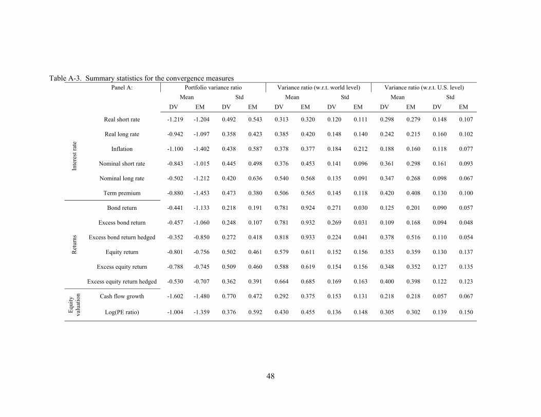
48

Table A-3. Summary statistics for the convergence measures Panel A: Portfolio variance ratio Variance ratio (w.r.t. world level) Variance ratio (w.r.t. U.S. level)

Mean Std Mean Std Mean Std

DV EM DV EM DV EM DV EM DV EM DV EM

Inte

rest

rat

e

Real short rate -1.219 -1.204 0.492 0.543 0.313 0.320 0.120 0.111 0.298 0.279 0.148 0.107

Real long rate -0.942 -1.097 0.358 0.423 0.385 0.420 0.148 0.140 0.242 0.215 0.160 0.102

Inflation -1.100 -1.402 0.438 0.587 0.378 0.377 0.184 0.212 0.188 0.160 0.118 0.077

Nominal short rate -0.843 -1.015 0.445 0.498 0.376 0.453 0.141 0.096 0.361 0.298 0.161 0.093

Nominal long rate -0.502 -1.212 0.420 0.636 0.540 0.568 0.135 0.091 0.347 0.268 0.098 0.067

Term premium -0.880 -1.453 0.473 0.380 0.506 0.565 0.145 0.118 0.420 0.408 0.130 0.100

Ret

urns

Bond return -0.441 -1.133 0.218 0.191 0.781 0.924 0.271 0.030 0.125 0.201 0.090 0.057

Excess bond return -0.457 -1.060 0.248 0.107 0.781 0.932 0.269 0.031 0.109 0.168 0.094 0.048

Excess bond return hedged -0.352 -0.850 0.272 0.418 0.818 0.933 0.224 0.041 0.378 0.516 0.110 0.054

Equity return -0.801 -0.756 0.502 0.461 0.579 0.611 0.152 0.156 0.353 0.359 0.130 0.137

Excess equity return -0.788 -0.745 0.509 0.460 0.588 0.619 0.154 0.156 0.348 0.352 0.127 0.135

Excess equity return hedged -0.530 -0.707 0.362 0.391 0.664 0.685 0.169 0.163 0.400 0.398 0.122 0.123

Equ

ity

valu

atio

n Cash flow growth -1.602 -1.480 0.770 0.472 0.292 0.375 0.153 0.131 0.218 0.218 0.057 0.067

Log(PE ratio) -1.004 -1.359 0.376 0.592 0.430 0.455 0.136 0.148 0.305 0.302 0.139 0.150

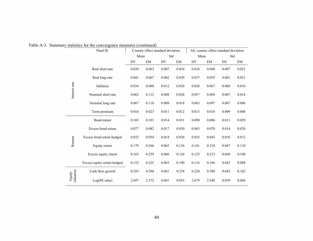
49

Table A-3. Summary statistics for the convergence measures (continued) Panel B: Country effect standard deviation Alt. country effect standard deviation

Mean Std Mean Std

DV EM DV EM DV EM DV EM

Inte

rest

rat

e Real short rate 0.039 0.063 0.007 0.034 0.034 0.048 0.007 0.021

Real long rate 0.041 0.067 0.002 0.029 0.037 0.055 0.001 0.021

Inflation 0.034 0.088 0.012 0.036 0.028 0.067 0.008 0.016

Nominal short rate 0.062 0.112 0.008 0.028 0.057 0.094 0.007 0.014

Nominal long rate 0.067 0.110 0.009 0.018 0.063 0.097 0.007 0.006

Term premium 0.016 0.023 0.011 0.012 0.013 0.018 0.009 0.008

Ret

urns

Bond return 0.103 0.101 0.014 0.031 0.090 0.086 0.011 0.029

Excess bond return 0.077 0.082 0.017 0.030 0.063 0.070 0.014 0.028

Excess bond return hedged 0.032 0.054 0.014 0.020 0.025 0.043 0.010 0.012

Equity return 0.179 0.266 0.065 0.126 0.141 0.218 0.047 0.110

Excess equity return 0.163 0.259 0.066 0.126 0.125 0.213 0.048 0.108

Excess equity return hedged 0.152 0.225 0.063 0.100 0.116 0.186 0.043 0.088

Equ

ity

valu

atio

n Cash flow growth 0.293 0.504 0.061 0.254 0.224 0.380 0.042 0.182

Log(PE ratio) 2.697 2.572 0.041 0.055 2.679 2.540 0.039 0.044

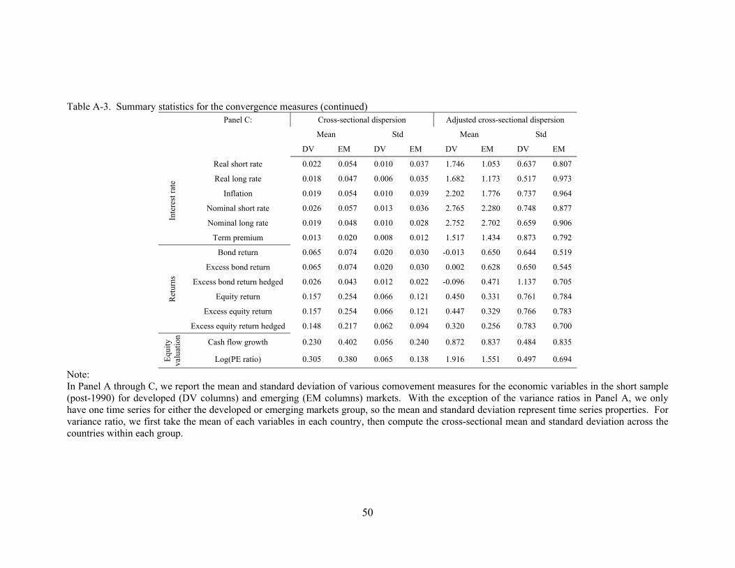
50

Table A-3. Summary statistics for the convergence measures (continued) Panel C: Cross-sectional dispersion Adjusted cross-sectional dispersion

Mean Std Mean Std

DV EM DV EM DV EM DV EM

Inte

rest

rat

e Real short rate 0.022 0.054 0.010 0.037 1.746 1.053 0.637 0.807

Real long rate 0.018 0.047 0.006 0.035 1.682 1.173 0.517 0.973

Inflation 0.019 0.054 0.010 0.039 2.202 1.776 0.737 0.964

Nominal short rate 0.026 0.057 0.013 0.036 2.765 2.280 0.748 0.877

Nominal long rate 0.019 0.048 0.010 0.028 2.752 2.702 0.659 0.906

Term premium 0.013 0.020 0.008 0.012 1.517 1.434 0.873 0.792

Ret

urns

Bond return 0.065 0.074 0.020 0.030 -0.013 0.650 0.644 0.519

Excess bond return 0.065 0.074 0.020 0.030 0.002 0.628 0.650 0.545

Excess bond return hedged 0.026 0.043 0.012 0.022 -0.096 0.471 1.137 0.705

Equity return 0.157 0.254 0.066 0.121 0.450 0.331 0.761 0.784

Excess equity return 0.157 0.254 0.066 0.121 0.447 0.329 0.766 0.783

Excess equity return hedged 0.148 0.217 0.062 0.094 0.320 0.256 0.783 0.700

Equ

ity

va

luat

ion

Cash flow growth 0.230 0.402 0.056 0.240 0.872 0.837 0.484 0.835

Log(PE ratio) 0.305 0.380 0.065 0.138 1.916 1.551 0.497 0.694

Note: In Panel A through C, we report the mean and standard deviation of various comovement measures for the economic variables in the short sample (post-1990) for developed (DV columns) and emerging (EM columns) markets. With the exception of the variance ratios in Panel A, we only have one time series for either the developed or emerging markets group, so the mean and standard deviation represent time series properties. For variance ratio, we first take the mean of each variables in each country, then compute the cross-sectional mean and standard deviation across the countries within each group.

51

B Decomposition of cross-sectional dispersion

Consider the sequence of the cross-sectional dispersion as:

∑ (B-1)

This statistic can be decomposed as follows:

∑

= ∑ ∑ 2 ∑ (B-2)

= A + B + C

Taking time series expectations, it follows that E[CSt2] = E[A] + E[B] + E[C] where

∑ ∑ (B-3)

2 ∑ ∑ 2 ∑ ∑

2 ∑ ∑ 2 ∑ ∑

0 2 ∑

2 (B-4)

∑

= ∑ ∑ 2 ∑

= ∑ ∑

(B-5)

where ∑ is the cross-sectional variance applied to country means. This

imples

(B-6)

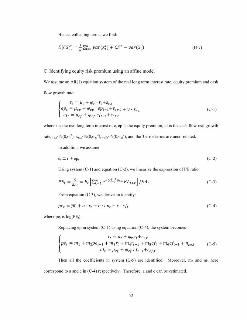
52

Hence, collecting terms, we find:

∑ (B-7)

C Identifying equity risk premium using an affine model

We assume an AR(1) equation system of the real long term interest rate, equity premium and cash

flow growth rate:

· ,· ,

· ,

· , (C-1)

where r is the real long term interest rate, ep is the equity premium, cf is the cash flow real growth

rate, εr,t~N(0,σr2), εep,t~N(0,σep

2), εcf,t~N(0,σcf2), and the 3 error terms are uncorrelated.

In addition, we assume

δt rt + ept (C-2)

Using system (C-1) and equation (C-2), we linearize the expression of PE ratio

∑ ∑ / (C-3)

From equation (C-3), we derive an identity:

· · · (C-4)

where pet is log(PEt).

Replacing ep in system (C-1) using equation (C-4), the system becomes

· ,

,

· ,

(C-5)

Then all the coefficients in system (C-5) are identified. Moreover, m3 and m5 here

correspond to a and c in (C-4) respectively. Therefore, a and c can be estimated.

53

Note that we cannot identify b and hence only get an affine function of the equity

premium:

· ̂ · (C-6)

For each country, we estimate a and c using an unrestricted OLS regression of the second

equation in (C-5) and construct the time series of the affine function of the equity premium afept.

Because afep is not the equity premium itself, we cannot use convergence measures that depend

on scale.