Global Omtimization

Yi Shang and Benjamin W. Wah University of Illinois, Urbana-Champaign

This training method

combines global and local

searches to find a good local

minimum. In benchmark com-

parisons against the best

global optimization

algorithms, it demonstrates

superior performance

improvement.

0018-9162/96/$5.00 0 1996 IEEE

earning in neural networks-whether supervised or unsuper- vised-is accomplished by adjusting the weights between con- nections in response to new inputs or training patterns. In

feed-forward neural networks, this involves mapping from an input space to an output space. That is, output 0 can be defined as a function of inputs I and connection weights W 0 = $ ( I , W), where $represents a mapping function.

Supervised learning involves finding a good mapping function-one that maps training patterns correctly and generalizes the mapping to test patterns not seen in training. This is done by adjusting weights Won links while fixing the topology and activation function. In other words, given a set of training patterns of input-output pairs { (II, D J , (I2, D J , . . . , (I,,,, D,,,)} and an error function E(W, I , D) , learning strives to minimize learning error E(w:

One popular error function is the squared-error function in which E(W, I,, 0,) = ($ (I( , w) -DJ2. SinceE(W) 2 0 for a given set of training patterns, if a W’ exists such that E(W’) = 0, then W’ is a global minimum; other- wise, the Wthat gives the smallestE(W) is the global minimum. The qual- ity of a learned network is measured by its error on a given set of training patterns and its (generalization) error on a given set of test patterns.

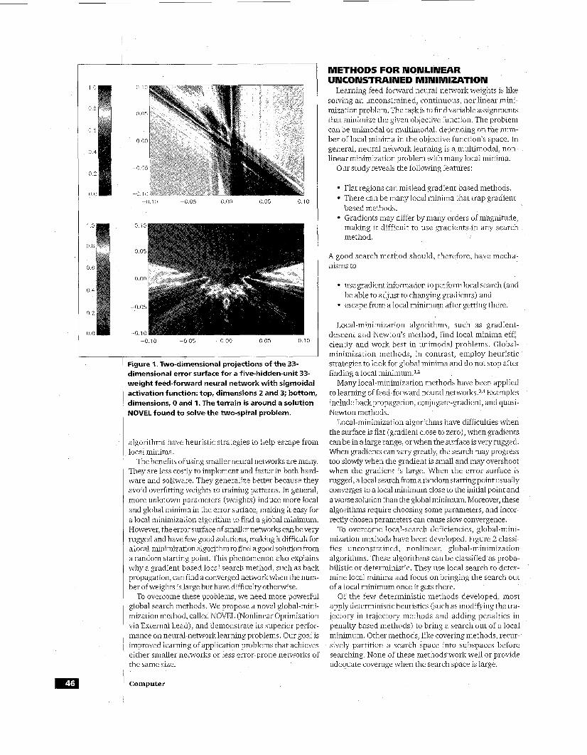
Supervised learning can be considered an unconstrained nonlinear minimization problem in which the objective function is defined by error function and the search space is defined by weight space. Unfortunately, the terrain modeled by the error function in its weight space can be extremelyrugged and have many local minima. This phenomenon is illus- trated in Figure 1, which shows two contour plots of the error surface around a local minimum along two dimension pairs. The top one shows a large number of small local minima; the bottom one shows large flat regions and steep slopes. Obviously, a search method that cannot escape from a local minimum will have difficulty in finding a solution that mini- mizes error function.

Many learning algorithms find their roots in function-minimization algorithms that can be classified as local- or global-minimization algo- rithms. Local-minimization algorithms, such as gradient-descent, are fast but usually converge to local minima. In contrast, global-minimization

March 1996

c 1 0

0 8

0 6

0 4

0 2

0 0

1 0

0 8

0 6

0 4

0 2

0 0

-0.10 -0 05 0 00 0 05 0.10

-0 10 -0 05 0 00 0 05 0 10

Figure 1. Two-dimensional projections of the 33- dimensional error surface for a five-hidden-unit 33- weight feed-forward neural network with sigmoidal activation function: top, dimensions 2 and 3; bottom, dimensions, 0 and 1. The terrain is around a solution NOVEL found to solve the two-spiral problem.

algorithms have heuristic strategies to help escape from local minima.

The benefits of using smaller neural networks are many. They are less costly to implement and faster in both hard- ware and software. They generalize better because they avoid overfitting weights to training patterns. In general, more unknown parameters (weights) induce more local and global minima in the error surface, making it easy for a local minimization algorithm to find a global "m. However, the error surface of smaller networks can be very rugged and have few good solutions, making it difficult for a local-minimization algorithm to fmd a good solunon from a random starting point. This phenomenon also explains why a gradient-based local search method, such as back propagation, can find a converged networkwhen the num- ber of weights is large but have difficulty otherwise.

To overcome these problems, we need more powerful global search methods. We propose a novel global-mini- mization method, called NOVEL (Nonlinear Optimization via External Lead), and demonstrate its superior perfor- mance on neural-network learning problems. Our goal is improved learning of application problems that achieves either smaller networks or less error-prone networks of the same size.

Computer

METHODS FOR NONLINEAR UNCONSTRAINED MlNlMlZATlON

Learning feed-forward neural-network weights is like solving an unconstrained, continuous, nonlinear mini- mization problem. The task is to find variable assignments that minimize the given objective function. The problem can be unimodal or multimodal, depending on the num- ber of local minima in the objective function's space. In general, neural network learning is a multimodal, non- linear minimization problem with many local minima.

Our study reveals the following features:

Flat regions can mislead gradient-based methods. There can be many local minima that trap gradient- based methods. Gradients may differ by many orders of magnitude, making it difficult to use gradients in any search method.

A good search method should, therefore, have mecha- nisms to

use gradient information to perform local search (and

* escape from a local minimum after getting there. be able to adjust to changing gradients) and

Local-minimization algorithms, such as gradient- descent and Newton's method, find local minima effi ciently and work best in unimodal problems. Global- minimization methods, in contrast, employ heuristic strategies to look for global minima and do not stop after finding a local

Many local-minimization methods have been applied to learning of feed-forward neural network^.^,^ Examples include back propagation, conjugate-gradient, and quasi- Newton methods.

Local-minimization algorithms have difficulties when the surface is flat (gradient close to zero), when gradients can be in a large range, or when the surface is very rugged. When gradients can vary greatly, the search may progress too slowly when the gradient is small and may overshoot when the gradient is large. When the error surface is rugged, a local search from a random starting point usually converges to a local minimum close to the initial point and a worse solution than the global minimum. Moreover, these algorithms require choosing some parameters, and incor- rectly chosen parameters can cause slow convergence.

To overcome local-search deficiencies, global-mini- mization methods have been developed. Figure 2 classi- fies unconstrained, nonlinear, global-minimization algorithms. These algorithms can be classified as proba- bilistic or deterministic. They use local search to deter- mine local minima and focus on bringing the search out of a local minimum once it gets there.

Of the few deterministic methods developed, most apply deterministic heuristics (such as modifymg the tra- jectory in trajectory methods and adding penalties in penalty-based methods) to bring a search odt of a local minimum. Other methods, like covering methods, recur- sively partition a search space into subspaces before searching. None of these methods work well or provide adequate coverage when the search space is large.

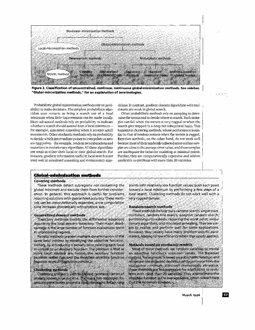
Figure 2. Classification of unconstrained, nonlinear, continuous global-minimization methods. See sidebar, "Global-minimization methods," for an explanation of terminologies.

Probabilistic global-minimization methods rely on prob- ability to make decisions. The simplest probabilistic algo- rithm uses restarts to bring a search out of a local minimum when little improvement can be made locally. More advanced methods rely on probability to indicate whether a search should ascend from a local minimum- for example, simulated annealing when it accepts uphill movements. Other stochastic methods rely on probability to decide which intermediate points to interpolate as new starting points-for example, random recombinations and mutations in evolutionary algorithms. All these algorithms are weak in either their local or their global search. For instance, gradient information useful in local search is not used well in simulated annealing and evolutionary algo-

rithms. In contrast, gradient-descent algorithms with mul- tistarts are weak in global search.

Other probabilistic methods rely on sampling to deter- mine the terrain and to decide where to search. Such strate- gies can fail when the terrain is very rugged or when the search gets trapped in a deep but suboptimal basin. This happens in clustering methods, whose performance is sim- ilar to that of random restarts when the terrain is rugged. Bayesian methods, on the other hand, do not work well because most of their randomly collected error-surface sam- ples are close to the average error value, and these samples are inadequate for behavior modeling at minimal points. Further, they are computationally expensive and seldom applicable to problems with more than 20 variables.

, Global-minimizdon methods Covering methods

These methods detect subregions not containing the global minimum and exclude them from further consider- ation. In general, this approach is useful for problems requiring solutions with guaranteed accuracy. These meth- ods can be computationally expensive, since computation time increases dramatically with problem size.

Generalized descent methods Trajectory methods modify the differential equations

describing the local descent trajectory. Their major disad- vantage is the large number of function evaluations spent in unpromising regions.

Penalty methods prevent multiple determination of the same local minima by modifying the objective function, namely, by introducing a penalty term relating each local minimum to an auxiliary function. The problem is that as more local minima are found, the auxiliary function becomes rather flat, and the modified objective function becomes more #iff icult to minimize.

clWte*methods Clustering analysis is used to prevent redetermination of

already known local minima, There are t w ~ strategies for grouping the points: around a focal minimum: Retain only

points with relatively low function values; push each point toward a local minimum by performing a few steps of a local search. Clustering methods do not work well with a very rugged terrain.

Random-search methods These methods include pure random search, single-start,

multistart, random line search, adaptive random search, partitioning into subsets, replacing the worst point, evolu- tionary algorithms, and simulated annealing. They are sim- ple to realize and perform well for some applications. However, they usually have many problem-specific para- meters, leading to low efficiency when improperly applied.

Methods basedon stochastic models Most of these methods use random variables to model

an objective function's unknown values. The Bayesian method, for example, is based on a stochastic function and minimizes the expected deviation of the estimate from the real global minimum. Although theoretically attractive, these methods are too expensive for application to prob- lems with more than 20 variables. They approximate the objective function in the average sense, which doesn't help find the minimum solution.

March 1996

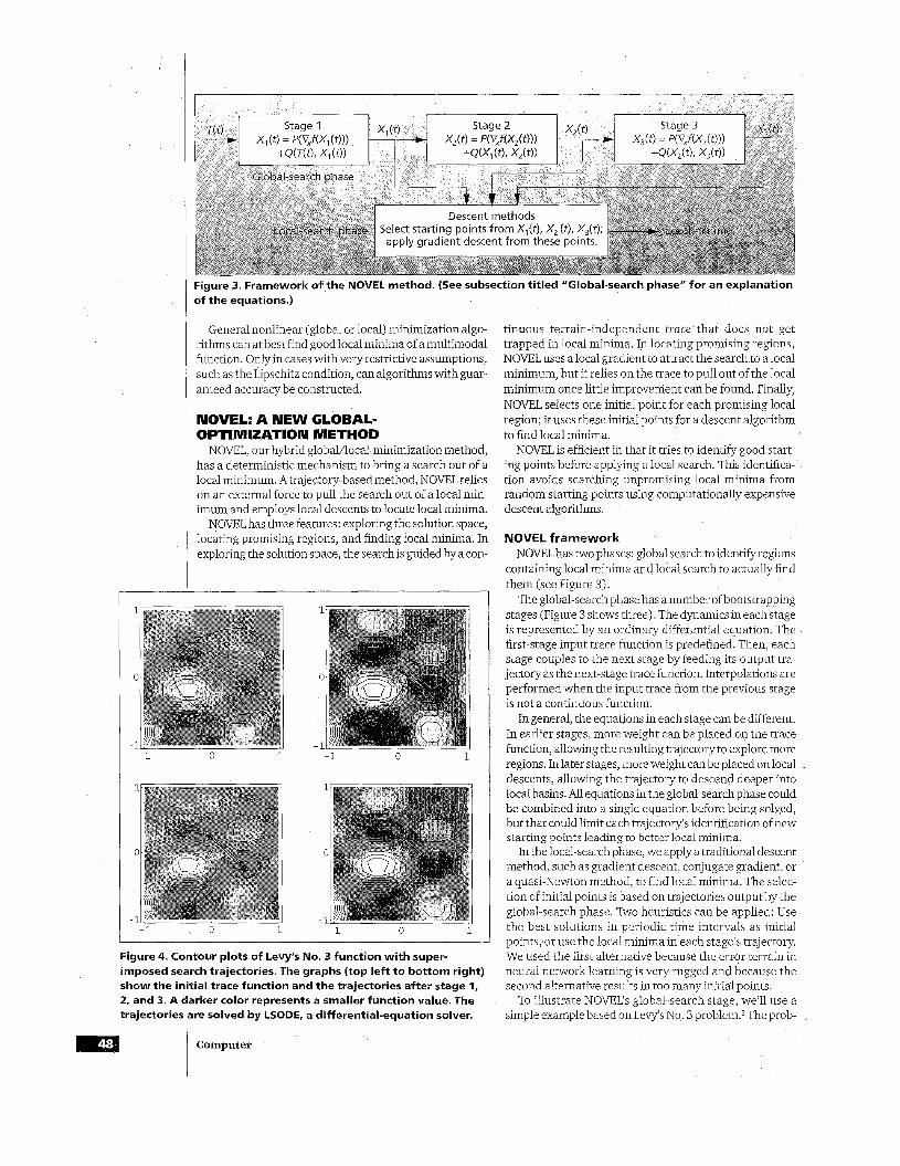
Figure 3. Framework of the NOVEL method. (See subsection titled “Global-search phase” for an explanation of the equations.)

General nonlinear (global or local) minimization algo- rithms can at best find good local minima of a multimodal function. Only in cases with very restrictive assumptions, such as the Lipschitz condition, can algorithms with guar- anteed accuracy be constructed.

NOVEL: A NEW GLOBAL- OPTIMIZATION METHOD

NOVEL, our hybrid global/local-minimization method, has a deterministic mechanism to bring a search out of a local minimum. A trajectory-based method, NOVEL relies on an external force to pull the search out of a local min- imum and employs local descents to locate local minima.

NOVEL has three features: exploring the solution space, locating promising regions, and finding local minima. In exploring the solution space, the search is guided by a con-

-1 0 1 -1 0 1

Figure 4. Contour plots of Levy’s No. 3 function with super- imposed search trajectories. The graphs (top left to bottom right) show the initial trace function and the trajectories after stage 1, 2, and 3. A darker color represents a smaller function value. The trajectories are solved by LSODE, a differential-equation solver.

Computer

tinuous terrain-independent trace that does not get trapped in local minima. In locating promising regions, NOVEL uses a local gradient to attract the search to a local minimum, but it relies on the trace to pull out of the local minimum once little improvement can be found. Finally, NOVEL selects one initial point for each promising local region; it uses these initial points for a descent algorithm to find local minima.

NOVEL is efficient in that it tries to identify good start- ing points before applying a local search. This identifica- tion avoids searching unpromising local minima from random starting points using computationally expensive descent algorithms.

NOVEL framework NOVEL has two phases: global search to identify regions

containing local minima and local search to actually find them (see Figure 3).

The global-search phase has a number of bootstrapping stages (Figure 3 shows three). The dynamics in each stage is represented by an ordinary differential equation. The first-stage input trace function is predefined. Then, each stage couples to the next stage by feeding its output tra- jectory as the next-stage trace function. Interpolations are performed when the input trace from the previous stage is not a continuous function.

In general, the equations in each stage can be different. In earlier stages, more weight can be placed on the trace function, allowing the resulting trajectory to explore more regions. In later stages, more weight can be placed on local descents, allowing the trajectory to descend deeper into local basins. All equations in the global-search phase could be combined into a single equation before being solved, but that could limit each trajectory’s identification of new starting points leading to better local minima.

In the local-search phase, we apply a traditional descent method, such as gradient descent, conjugate gradient, or a quasi-Newton method, to find local minima. The selec- tion of initial points is based on trajectories output by the global-search phase. Two heuristics can be applied: Use the best solutions in periodic time intervals as initial points, or use the local minima in each stage’s trajectory. We used the first alternative because the error terrain in neural network learning is very rugged and because the second alternative results in too many initial points.

To illustrate NOVEL‘S global-search stage, we’ll use a simple example based on Levy‘s No. 3 p r ~ b l e m . ~ The prob-

lem involves finding the global minimum of a function of two variables,~, andx,:

i = l j=1

(2)

Figure 4 shows the 2D contour plots of this function and the NOVEL search trajectories. In the range shown, the func- tion has three local minima, one ofwhich is the global min- imum. Using a search range of [-1,1] in each dimension, we start NOVEL from (0,O) and run it until logical time t = 5. Although the trace functionvisits all three basins, it touches only the basin with the global minimum. The trajectories are pulled closer to the local basins after stages 1,2, and 3. Following the trajectories, NOVEL identifies three basins with local minima. A set of minimal points from each tra- jectory provides initial points for local search.

Global-search phase AssumefQ with gradient V,f (X) is to be minimized,

wherex = (x,, x,, . . ., x,) are variables. There may be sim- ple bounds like x, E [a,, b,], where a,, b,, i = 1, ..., n, are real numbers.

Each stage in the NOVEL global-search phase defines a trajectoryX(t) = (x, (t) , . . ., x, ( t ) ) that is governed by the following ordinary differential equation:

where tis the autonomous variable; T, the trace function, is a function oft; andP and Q are general nonlinear func- tions. This equation specifies a trajectory through vari- able space x. It has two components: P(Vxf(x)) lets the gradient attract the trajectory to a local minimum, and Q (T ,x ) lets the trace functionlead the trajectoryout of the local minimum.

P and Q can have various forms. We used a simple form

where pg and pt are constant coefficients. Finding the global minima, without terrain knowledge,

requires a trace function that covers the search space uni- formly. There are two alternatives: Divide the space into subspaces and search one extensively before going to another, or search the space from coarse to fine. Numerous dimensions can make the first approach impractical, so we chose the second approach and, after much experimenta- tion, designed a nonperiodic, analytical trace function:

where i represents the ith dimension, p is a coefficient specifying the range, and n is the number of dimensions.

Given Equation 4, we can apply various numerical approaches to evaluate the ordinary differential equation. We have used both a differential-equation solver and a dif-

ference-equation solver. The differential-equation solver we have used is LSODE

(Livermore Solver for Ordinary Differential Equations) .6 It solves Equation 4 to a prescribed degree of accuracy, but it is computationally expensive, especially for a large num- ber of variables. It also requires the true gradient, so neural network learning must be done in an epochwise rather than patternwise mode.

The second approach is to discretize Equation 4 and use a firrite-difference equation solver. The difference equa- tion derived is

where 6t is the step size. A large S t causes a large stride of variable modification, possibly resulting in oscillations. On the other hand, a small 6 t requires a longer computation time to traverse the same distance. This approach is fast and allows both patternwise and epochwise learning. However, solutions maybe slightlyworse than those found by LSODE.

EXPERIMENTAL RESULTS In general, NOVEL finds better results than other global-

minimization algorithms in the same amount of time. In this section, we compare NOVEL‘S performance on several benchmarks with that of other good methods for global minimization. (See sidebar, “Benchmark problems stud- ied in our experiments.”)

Two-spiral problem The two-spiral problem is a difficult classification prob-

lem. Published results include training feed-forward net- works using back propagation, cascade correlation (Cascor7), and projection pursuit learning.* The smallest network is believed to have nine hidden units with 75 weights trained by Cascor.

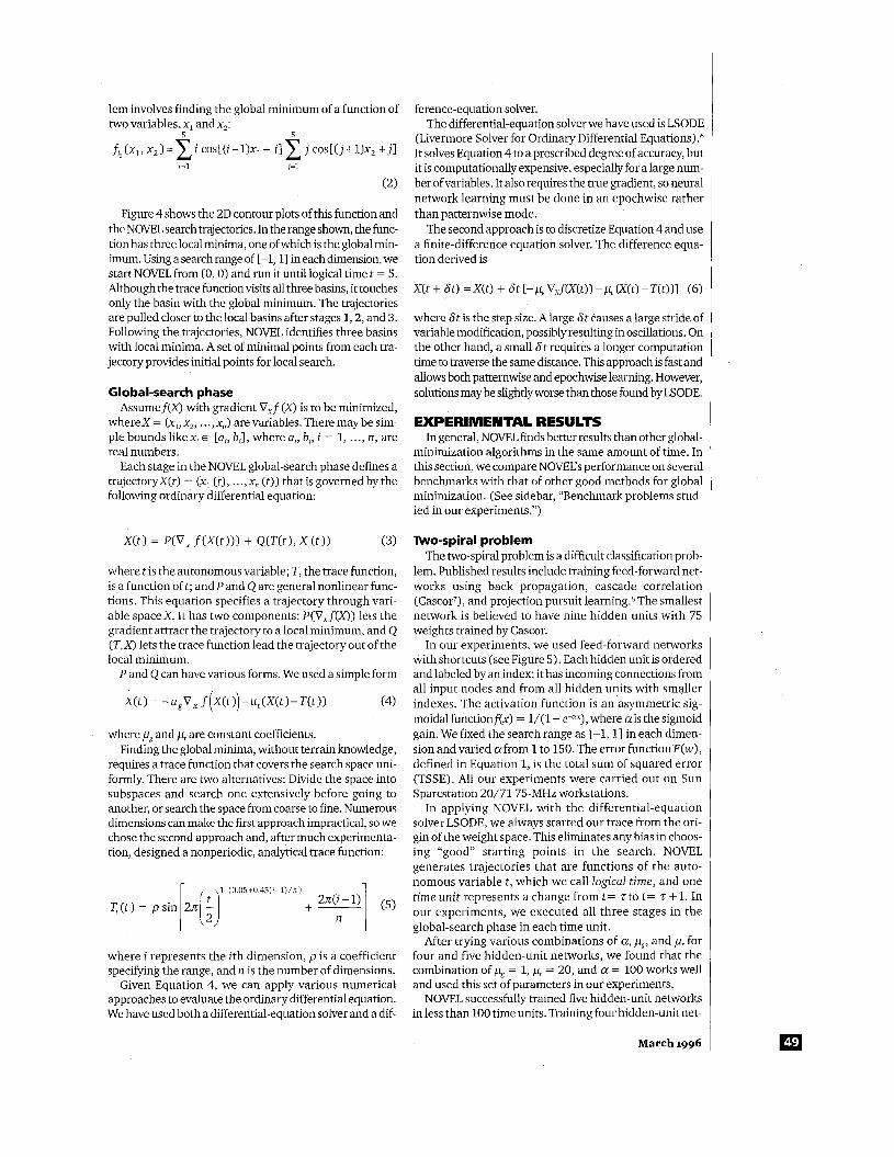
In our experiments, we used feed-forward networks with shortcuts (see Figure 5). Each hidden unit is ordered and labeled by an index; it has incoming connections from all input nodes and from all hidden units with smaller indexes. The activation function is an asymmetric sig- moidal functionf(x) = 1/(1+ e-ax), where ais the sigmoid gain. We fixed the search range as [-1,1] in each dimen- sion and varied afrom 1 to 150. The error function E(w), defined in Equation 1, is the total sum of squared error (TSSE). All our experiments were carried out on Sun Sparcstation 20/7175-MHz workstations.

In applying NOVEL with the differential-equation solver LSODE, we always started our trace from the ori- gin of the weight space. This eliminates any bias in choos- ing “good” starting points in the search. NOVEL generates trajectories that are functions of the auto- nomous variable t , which we call logical time, and one time unit represents a change from t= z to t= z +l. In our experiments, we executed all three stages in the global-search phase in each time unit.

After trying various combinations of a, pg, and pr for four and five hidden-unit networks, we found that the combination of pg = 1, pc = 20, and a = 100 works well and used this set of parameters in our experiments.

NOVEL successfully trained five hidden-unit networks in less than 100 time units. Training four hidden-unit net-

March 1996

Benchmark problems studied in our experiments We used the following benchiiiarks in our expeyi-

ments All benchmarks were obtained from kp.cs cmu edu in directory /afs/cs/project/connect/bench.

Two-spiral problem This problem discriminates between two sets of

training points that lie on two distinct spirals in the x-y plane. Each spiral has 94 input-output pairs in both the training and test sets.

Sonar problem This problem discriminates between sonar signals

bounced off a metallic cylinder and those bounced off a roughly cylindrical rock. We used the training and test samples in ”aspect angle-dependent” exper- iments.

output is the smallest among the distances from the actual output to al l possible target outputs.

10-parity problem This problem trains a network that computes the

modulo-two sum of 10 binary digits There are 1,024 training patterns and no test patterns

Ne- problem This problem trains a network to produce proper

phonemes, given a string of letters as input. NetTalk‘s data set contains20,008 English words. We used the same network settings and unary encoding as in Sejgowski and Rosenberg‘s experiments,’ the 1,000 most common English words as the trai

’

Figure 5. Neural network structure for the two-spiral problem.

works is more difficult. After running NOVEL for 19 hours, we found a solution with TSSE of 4.0. Using this solution as a new starting point, we executed NOVEL for another 15 hours and found a 2.0 solution, which is 99 percent cor- rect. Again, starting with this solution and running NOVEL for another 10 hours, we found a solution that is 100 per- cent correct. The second figure in the first row of Figure 6 shows how the best four hidden-unit network found clas- sifies the 2D space.

Next, we compare NOVEL‘S performance with that of simulated annealing, evolutionary algorithms, cascade correlation with multistarts, gradient descent with mul- tistarts, and a truncated Newton’s method with multi- starts. (For a brief description of each method, see the sidebar, “Good global minimization methods for neural network training.”) To allow a fair comparison, we ran all

Computer

methods for the same amount of time using the same net- work structure.

The simulated annealing program used in our experi- ments is Simann from netlib.9

We experimented with various temperature scheduling factors RT, function evaluation factors NT, and search ranges. The best results were achieved when RT = 0.99, NT = 5 n, and the search range is [-2.0,2.0].

We have also studied two evolutionary algorithms: Michalewicz’s Genocop (genetic algorithm for numerical optimization for constrained problems)10 and Sprave’s Lice (linear cellular evolution) .I1 Genocop aims to find an objective-function global minimum under linear con- straints. After trying various search ranges and popula- tion sizes, we found that range [-0.5,0.5] and size 100 n give the best results.

Figure 6. Two-dimensional classification graphs for the two-spiral problem by three (first column), four (second column), f ive (third column), and six (fourth column) hidden-unit neural networks trained by NOVEL (upper row) and Simann (lower row). Parameters for NOVEL are pLS= 1, = 20, and a = 100. Parame- ters for Simann are R f = 0.99, NT = 5 n, and the search range is [-2.0.2.01. The crosses and circles represent the training patterns.

March 1996

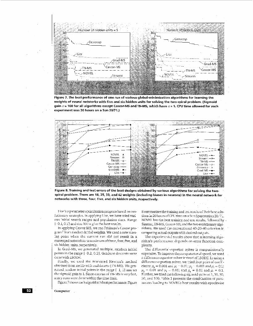
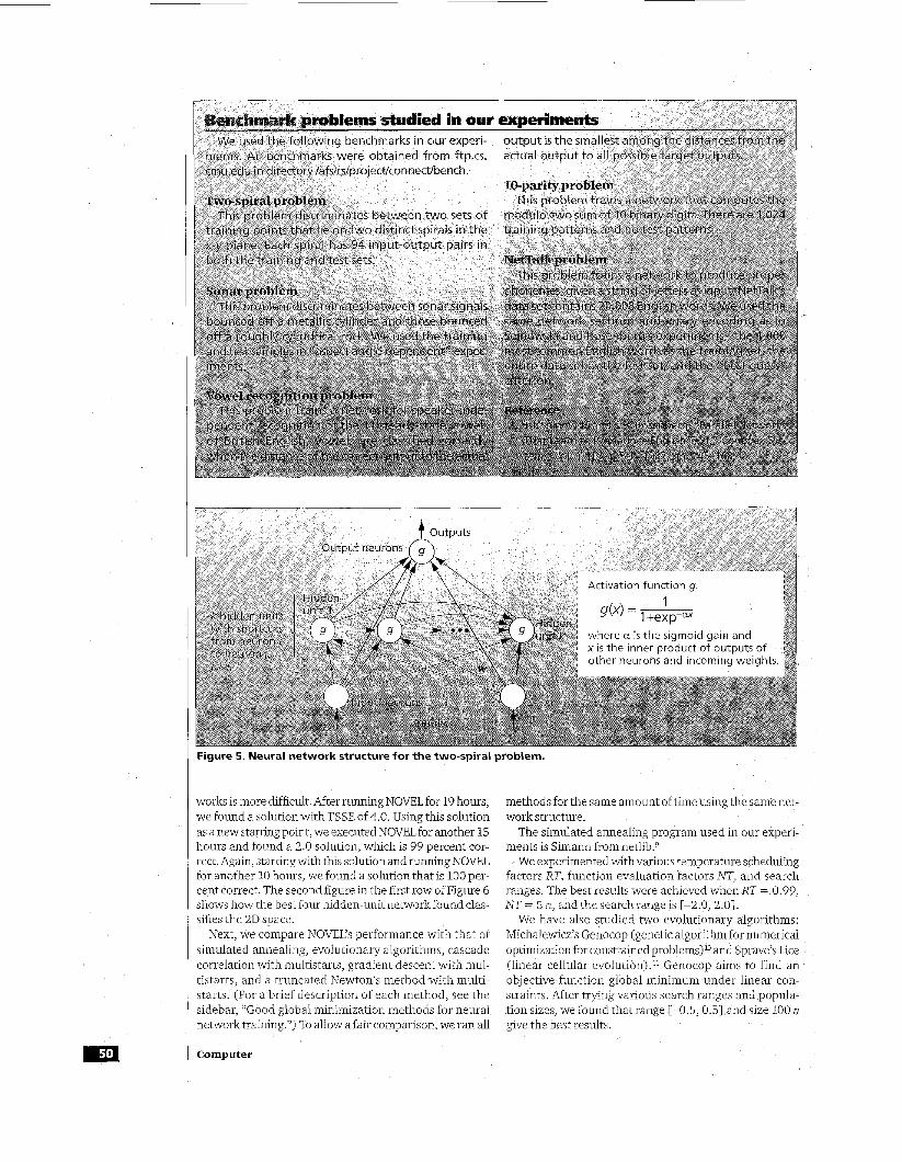
Figure 7. The best performance of one run of various global-minimization algorithms for learning the weights of neural networks with five and six hidden units for solving the two-spiral problem. (Sigmoid gain a = 100 for all algorithms except Cascor-MS and TN-MS, which have a = 1. CPU time allowed for each experiment was 20 hours on a Sun 20/71.)

Figure 8. Training and test errors of the best designs obtained by various algorithms for solving the two- spiral problem. There are 18,25,33, and 42 weights (including biases in neurons) in the neural network for networks with three, four, five, and six hidden units, respectively.

Lice is a parameter optimization program based on evo- lutionary strategies. In applying Lice, we have tried vari- ous initial search ranges and population sizes. Range [-0.1,0.1] and size 100 n give the best results.

In applying Cascor-MS, we ran Fahlman's Cascor pro- gram7 from random initial weights. We used a new start- ing point when the current run did not result in a converged network for a maximum of three, four, five, and six hidden units, respectively.

In Grad-MS, we generated multiple, random initial points in the range [-0.2, 0.21. Gradient descents were done with LSODE.

Finally, we used the truncated Newton's method obtained from netlib with multistarts (TN-MS). We gen- erated random initial points in the range [-1, 11 and set the sigmoid gain to 1. Since one run of TN-MS is very fast, many runs were done within the time limit.

Figure 7 shows each algorithm's best performance. Figure

8 summarizes the training and test results of their best solu- tions in 20 hours of CPU time on a Sun Sparcstation 20/71. NOVEL has the best training and test results, followed by Si", TN-MS, Cascor-MS, and the two evolutionary algo- rithms. We used the conventional 40-20-40 criterion in comparing actual outputs with desired outputs.

The experimental results show that a learning algo- rithm's performance depends on error-function com- plexity.

The differential-equation solver is computationally expensive. To improve thecomputational speed, we used a difference-equation solver instead of LSODE. In using a difference-equation solver, we tried four pairs of coeffi- cients: pg = 0.001 andpr = 0.01; pz = 0.001 and pc = 0.1; pz = 0.01 and pr = 0.01; and pz = 0.01 and p, = 0.1. Further, we tried the following sigmoid gains a: 1,10,30, 50, and 100. Table 1 presents the combination of para- meters leading to NOVEL'S best results with epochwise

Computer

training. The difference-equation solver is about 10 times faster than LSODE, but its solution quality is slightly worse.

Results on other benchmarks The network topologies used in these experiments with

other benchmarks are layered feed-forward networks without shortcuts (to be consistent with what other researchers have used), and the goal is to minimize the total sum of squared errors. Other setups are similar to those described for the two-spiral problem.

For the sonar problem, we applied NOVEL with a dif- ference-equation solver, TN-MS, Simann, and back prop- agation. As found by D i ~ o n , ~ TN runs much faster than epochwise back propagation and achieves comparable solutions. Simann is one order of magnitude slower than TN-MS and NOVEL with a difference-equation solver, and the results are not better. For these reasons, we describe only the results for TN-MS and NOVEL using a difference- equation solver. TN is used in the local-search phase of NOVEL.

Table 2 shows the best solutions of both algorithms that achieve the highest percentage of correctness on the sonar problem’s test patterns. Our results show that NOVEL improved test accuracy by 1-4 percent.

All results in Table 2 were run under similar conditions and time limits. In particular, NOVEL always started from

the origin and searched in the range [-1,1] for eachvari- able, using some combinations of sigmoid gains from the set { 1,10,30,50,100,300} and (pg, ,uJ from the set {(lo, l), (1, 11, (1,0.1), (O . l ,O . l ) , (0.1,1), (O.l,O.Ol), (0.01, O.l)}. TN-MS was run using different combinations of random initial points in search ranges from the set { E-0.1, 0.11, [-0.2, 0.21, [-0.5, 0.51, [-1, 11 } and the same sig- moid gains as in NOVEL. In TN-MS + NOVEL, NOVEL always started from the best result of TN-MS using the same sigmoid gain when TN-MS was run. In solving the NetTalkproblem, the sigmoid gain is set to 1. NOVEL used learning rates of 1 and 2 and a momentum of 0.1. Back propagation generated its initial point in the range [-0.5, 0.51, using a momentum of 0.1 and learning rates from the set {0.5,1,2,4,8,16).

We attribute NOVEL’S superiority in finding better local minima to its global-search stage. Since the func- tion searched is very rugged, it is important to avoid probing from many random starting points and to iden- tify good basins before committing expensive local descents. However, multistart algorithms may provide good starting points for NOVEL.

On the vowel-recognition problem, Table 2 shows that NOVEL improves training compared with TN-MS, but per- forms slightlyworse in testing when there are two hidden units. TN-MS + NOVEL also improved training compared with TN-MS.

March 1996

On the 10-parity problem, using a setup similar to the one described for the sonar problem, NOVEL improved the learning results obtained by TN-MS.

In the last application, the NetTalk problem, the num- ber of weights and training patterns is very large, so we used patternwise learning when applying back propaga- tion (as in Sejnowski and Rosenberg’s12 original experi- ments).

NetTalk’s large number of weights precluded using any method other than patternwise mode in the global-search phase and patternwise back propagation in the local- search phase. Even so, veryfew (logical) time units could be simulated, and our designs perform better in training but sometimes worse in testing. To find better designs, we took the best designs obtained by patternwise back prop- agation and applied NOVEL. Table 2 shows improved learning results but worse testing results. The poor test- ing results are probably due to the small number of time units that NOVEL ran.

In short, NOVEL’S training results are always better than or equal to those of TN-MS but are occasionally slightly worse in testing. We attribute this to the time constraint and the excellence of solutions already found by existing methods. In general, improving solutions that are close to the global minima is difficult, often requiring exponential time unless a better search method is used.

ALTHOUGH WE mm DEMONSTRATED N O W s power in solv- ing some neural network benchmarks, its applicability to other benchmarks and general nonlinear optimization problems needs further study. In particular, we need to study new trace functions that cover the search space from coarse to fine, their search range, the relative weights between local descent and affinity to the traveling trace, parallel processing of NOVEL, combining NOVEL with other local/global-search methods, and applying NOVEL to other problems.

In short, NOVEL represents a significant advance in supervised learning of feed-forward neural networks and optimization of general high-dimensional nonlinear con- tinuous functions. I

Acknowledgment This research was supported in part by National Science

Foundation Grant MIP 92-18715 and in part by Joint Services Electronics Program Contract N00014-90-5-1270,

Programs developed for this article can be accessed through the World Wide Web at http://manip.crhc.uiuc. edu.

4. L.C.W. Dixon, “Neural Networks and Unconstrained Opti- mization,’’ in Algorithmsfor Continuous Optimization: The State of the Art, E. Spedicato, ed., Kluwer Academic, The Netherlands, 1994, pp. 513-530.

5. A.V. Levy et al., Topics in Global Optimization, Lecture Notes in Mathematics No. 909, Springer-Verlag, New York, 1981.

6. A.C. Hindmarsh, “ODEPACK, a,Systematized Collection of ODE Solvers,”in Scientijk Computing (R.S. Stepleman, ed.), North Holland, Amsterdam, 1983, pp. 55-64.

7. S.E. Fahlman and C. Lebiere, “The Cascade-Correlation Learning Architecture,” inndvances in Neural Information Processing Systems 2, D.S. Touretzky, ed., Morgan Kaufmann, SanMateo, Calif., 1990, pp. 524-532.

8. J. Hwang et al., “Regression Modeling in Back-Propagation and Projection Pursuit Learning,” IEEE Trans. Neural Net- works, Vol. 5, May 1994, pp. 1-24.

9. A. Corana et al., “Minimizing Multi-ModalFunctions of Con- tinuousvariables with the Simulated Annealing Algorithm,” ACMTrans. MuthematicalSoftware, Vol: 13, No. 3,1987, pp.

10. 2. Michalewicz, Genetic Algorithms + Data Structure = Evo- lution Programs, Springer-Verlag, New York, 1994.

11. 3. Sprave, “Linear Neighborhood Evolution Strategies,” Proc. ThirdAnn. Con$ Evolutionary Programming, World Scientific, 1994.

12. T.J. Sejnowski and C.R. Rosenberg, “Parallel Networks That Learn to Pronounce English Text,” Complex Systems, Vol. 1, No. 1, Feb. 1987, pp. 145-168.

262-280.

Yi Shang is a PhD student in the Department of Computer Science of the University of Illinois, Urbana-Champaign. His research interests are in optimization, machine learning, neural networks, genetic akorithms, parallelprocessing, and image processing. He received his BSfrom the University of Science and Technologyof China and his MS in computerscil encefrom the Institute of Computing Technology, Academia Sinica, Beijing, China, in 1991.

Benjamin W. Wah is a professor in the Department ofElectrical and ComputerEngineering and the Coordinated Science Laboratory, University of Illinois, Urbana-Champaign. His current research interests are parallel and distributed processing, knowledge engineering, and optimization. He is editor-in-chief ofthe IEEE Transactions on Knowledge and Data Engineering and serves on the editorial boards ofInfor- mation Sciences, International Journal on Artificial Intel- ligence Tools, and Journal of VLSI Signal Processing. He is an IEEE fellow.

Readers can contact the authors at the Coordinated Science Laboratory, University of Illinois, 1308 West Main St., Urbana, IL 61801. Their e-mail addresses are ,{shang, wah)@manip. crhc. uiuc. edu and http://manip. crhc. uiuc. edu.

References 1. A. Torn and A. Zilinskas, Global Optimization, Springer-Ver-

lag, New York, 1987. 2. D.G. Luenberger, Linear andNonlinear Programming, Addi-

son-Wesley, Reading, Mass., 1984. 3. R. Battiti, “First- and Second-Order Methods for Learning:

Between Steepest Descent and Newton’s Method,” Neural Computation, Vol. 4, No. 2,1992, pp. 141-166.

Computer