SANDIA REPORT SAND2012-2389 Unlimited Release Printed March 2012

Global Horizontal Irradiance Clear Sky Models: Implementation and Analysis Matthew J. Reno, Clifford W. Hansen, Joshua S. Stein Prepared by Sandia National Laboratories Albuquerque, New Mexico 87185 and Livermore, California 94550 Sandia National Laboratories is a multi-program laboratory managed and operated by Sandia Corporation, a wholly owned subsidiary of Lockheed Martin Corporation, for the U.S. Department of Energy's National Nuclear Security Administration under contract DE-AC04-94AL85000. Approved for public release; further dissemination unlimited.

2

Issued by Sandia National Laboratories, operated for the United States Department of Energy by Sandia Corporation. NOTICE: This report was prepared as an account of work sponsored by an agency of the United States Government. Neither the United States Government, nor any agency thereof, nor any of their employees, nor any of their contractors, subcontractors, or their employees, make any warranty, express or implied, or assume any legal liability or responsibility for the accuracy, completeness, or usefulness of any information, apparatus, product, or process disclosed, or represent that its use would not infringe privately owned rights. Reference herein to any specific commercial product, process, or service by trade name, trademark, manufacturer, or otherwise, does not necessarily constitute or imply its endorsement, recommendation, or favoring by the United States Government, any agency thereof, or any of their contractors or subcontractors. The views and opinions expressed herein do not necessarily state or reflect those of the United States Government, any agency thereof, or any of their contractors. Printed in the United States of America. This report has been reproduced directly from the best available copy. Available to DOE and DOE contractors from U.S. Department of Energy Office of Scientific and Technical Information P.O. Box 62 Oak Ridge, TN 37831 Telephone: (865) 576-8401 Facsimile: (865) 576-5728 E-Mail: reports@adonis.osti.gov Online ordering: http://www.osti.gov/bridge Available to the public from U.S. Department of Commerce National Technical Information Service 5285 Port Royal Rd. Springfield, VA 22161 Telephone: (800) 553-6847 Facsimile: (703) 605-6900 E-Mail: orders@ntis.fedworld.gov Online order: http://www.ntis.gov/help/ordermethods.asp?loc=7-4-0#online

3

SAND2012-2389 Unlimited Release

Printed March 2012

Global Horizontal Irradiance Clear Sky Models: Implementation and Analysis

Matthew J. Reno, Clifford W. Hansen, Joshua S. Stein Photovoltaics and Grid Integration Department

Sandia National Laboratories P.O. Box 5800

Albuquerque, New Mexico 87185-1033

Abstract

Clear sky models estimate the terrestrial solar radiation under a cloudless sky as a function of the solar elevation angle, site altitude, aerosol concentration, water vapor, and various atmospheric conditions. This report provides an overview of a number of global horizontal irradiance (GHI) clear sky models from very simple to complex. Validation of clear-sky models requires comparison of model results to measured irradiance during clear-sky periods. To facilitate validation, we present a new algorithm for automatically identifying clear-sky periods in a time series of GHI measurements. We evaluate the performance of selected clear-sky models using measured data from 30 different sites, totaling about 300 site-years of data. We analyze the variation of these errors across time and location. In terms of error averaged over all locations and times, we found that complex models that correctly account for all the atmospheric parameters are slightly more accurate than other models, but, primarily at low elevations, comparable accuracy can be obtained from some simpler models. However, simpler models often exhibit errors that vary with time of day and season, whereas the errors for complex models vary less over time.

4

ACKNOWLEDGMENTS Irradiance data used for this analysis were obtained from a number of sources that deserve acknowledgment:

• National Renewable Energy Laboratory’s (NREL) Measurement and Instrumentation Data Center (MIDC);

• National Oceanic and Atmospheric Administration (NOAA) Surface Radiation (SURFRAD) Network;

• Las Vegas Valley Water District, Las Vegas, NV.

5

CONTENTS

1. Introduction ................................................................................................................................ 9

2. Background .............................................................................................................................. 11 2.1. Solar Position ................................................................................................................... 11 2.2. Extraterrestrial Radiation ................................................................................................. 13 2.3. Very Simple Models for Determining the Irradiance on Clear Day ................................ 14 2.4. Simple Models for Determining the Global Horizontal Irradiance on a Clear Day ........ 16 2.5. Complex Models for Determining the Global Horizontal Irradiance on a Clear Day ..... 17 2.6. Clear Sky Models Fit to Measured Data .......................................................................... 19 2.7. Linke Turbidity Models ................................................................................................... 20 2.8. Air Mass Models .............................................................................................................. 21 2.9. Review of Previous Analysis of Clear Sky Models ......................................................... 23

3. Detection Of Clear periods in GHI Measurements ................................................................... 27 3.1. Background ...................................................................................................................... 27 3.2. Criteria for Identifying Clear Periods .............................................................................. 28

3.2.1. Criteria for Detecting Clear-Sky Periods ........................................................... 28 3.2.2. Moving Window Method for Classifying Individual Measurements. ............... 32 3.2.3. Threshold Values for Criteria ............................................................................. 34

3.3. Iterative Process for Improved Detection of Clear Days ................................................. 36 3.4. Visual Verification of Clear Sky Detection ..................................................................... 37

4. Analysis of Clear Sky Models .................................................................................................. 41 4.1. Evaluation Criteria ........................................................................................................... 41 4.2. Irradiance data .................................................................................................................. 41 4.3. Model Analysis ................................................................................................................ 43

4.3.1. Models Under Consideration .............................................................................. 43 4.3.2. Average Model Error .......................................................................................... 43 4.3.3. Dependence of Model Error on Zenith Angle .................................................... 44 4.3.4. Dependence of Model Error on Time of Day and Time of Year ....................... 47 4.3.5. Dependence of Model Error on Location ........................................................... 52 4.3.6. Dependence of Model Error on Elevation .......................................................... 55

5. Conclusions ............................................................................................................................... 57

6. References ................................................................................................................................. 60

FIGURES Figure 1. Error in zenith angle from ASCE, Spencer, and SOLPOS models relative to SPA for equinoxes and solstices at Albuquerque, NM. .............................................................................. 13 Figure 2. Extraterrestrial radiation for ASCE, Spencer, and SOLPOS model for each day in 2010........................................................................................................................................................ 14 Figure 3. Results of six very simple clear sky GHI models solely dependent on zenith angle .... 16 Figure 4. Example global map of Linke turbidity......................................................................... 21 Figure 5. Graph of AM models at high zenith angles ................................................................... 23

6

Figure 6. Example of motivation for mean irradiance criterion for clear sky detection ............... 29 Figure 7. Examples of motivation for max value criterion for clear sky detection ...................... 29 Figure 8. Examples of motivation for line length criterion for clear sky detection ...................... 30 Figure 9. Example of motivation for variance of slope criterion for clear sky detection ............. 31 Figure 10. Example of motivation for maximum deviation from clear sky slope criterion ......... 32 Figure 11. Satellite Image of Clark Station, NV ........................................................................... 33 Figure 12. Measured GHI at Clark Station showing effect of power lines................................... 33 Figure 13. Measured GHI at Clark Station showing effect of a pole ........................................... 34 Figure 14. Line length of GHI in a 10-minute moving window on a clear day............................ 35 Figure 15. Line length of GHI in a 10-minute moving window on a cloudy day ........................ 35 Figure 16. Variance of the slopes of GHI in a 10-minute moving window on a clear day .......... 36 Figure 17. Variance of slopes of GHI in a 10-minute moving window on a cloudy day ............. 36 Figure 18. Flow chart for adaptive clear time detection algorithm ............................................... 37 Figure 19. Visual representation of clear sky detection. Measured irradiance is in blue, with red markers signifying minutes identified as clear. ............................................................................ 38 Figure 20. Visual representation of clear sky detection. Measured irradiance is in blue, with red markers signifying instants identified as clear. ............................................................................. 39 Figure 21. Measurement sites used in the analysis ....................................................................... 42 Figure 22. Average RMSE and MBE as a percentage of measured irradiance for each clear sky model at all sites............................................................................................................................ 44 Figure 23. Measured GHI vs. predicted GHI for each clear sky model ....................................... 45 Figure 24. Examples of clear sky model GHI output for NREL, Golden, CO, for two days (10/15/2008 and 10/28/2008). ....................................................................................................... 46 Figure 25. Clear sky models vs. zenith angle of the sun ............................................................... 46 Figure 26. Dependence of model error on zenith angle ................................................................ 47 Figure 27. Average error for each clear sky model by time of day .............................................. 48 Figure 28. Average error for each clear sky model by time of day, with error bars ..................... 49 Figure 29. Average monthly error for each clear sky model throughout the year ........................ 50 Figure 30. Average monthly error for each clear sky model throughout the year with error bars 51 Figure 31. Average error (W/m2) for each clear sky model for each hour and month ................. 52 Figure 32. RMSE for each site and each clear sky model ............................................................ 53 Figure 33. RMSE for clear sky models ......................................................................................... 54 Figure 34. Range of RMSE at each site for clear sky models ...................................................... 54 Figure 35. Results for eight clear sky models in Albuquerque, NM ............................................ 55 Figure 36. Results for eight clear sky models for Fort Apache station in Las Vegas, NV ........... 55 Figure 37. Dependence of model error (MBE) on site elevation .................................................. 56 Figure 38. Dependence of model error (RMSE) on site elevation ............................................... 56

TABLES Table 1. Summary of input parameters for complex clear sky models. ....................................... 19 Table 2. Table of irradiance measurement sites and number of detected clear days .................... 42

7

NOMENCLATURE AM Air Mass AOD Aerosol Optical Depth ASCE American Society of Civil Engineers CSI Clear Sky Irradiance DNI Direct Normal Irradiance DOE Department of Energy DOY Day of Year GHI Global Horizontal Irradiance MBE Mean bias error MIDC Measurement and Instrumentation Data Center NOAA National Oceanic & Atmospheric Administration NREL National Renewable Energy Laboratory NSRDB National Solar Radiation Database OMI Ozone Monitoring Instrument PSP Precision Spectral Pyranometer RMSE Root mean square error SNL Sandia National Laboratories SPA Solar Position Algorithm SRRL Solar Radiation Research Laboratory SURFRAD Surface Radiation WRR World Radiation Reference

8

9

1. INTRODUCTION

The terrestrial solar irradiance on a clear day has been highly studied and is a function of the solar elevation angle, site altitude, aerosol concentration, water vapor, and various other atmospheric conditions [1, 2]. As irradiance is a measure of the power of sunlight (W/m2), this information can be used to model the general maximum output of a solar photovoltaic system for any given day and location. Monthly or daily insolation (W-hr/m2) data is required to conduct feasibility studies for solar energy systems, but ground irradiance measurement sites are not always available, requiring the use of models to estimate irradiance in lieu of measurements [3]. Clear sky models are essential to estimating irradiance levels. Clear sky models are also used to calculate a cloudiness index or clearness index. In order to accurately calculate these indices, a well-calibrated clear sky model must be used for the location. Forecasting and variability analyses both rely on converting irradiance (W/m2) into a measure of percentage of power reaching the ground compared to maximum possible power for that location, date, and time. Clouds do not decrease the irradiance by a fixed amount (W/m2); instead they attenuate the sunlight by a certain percentage for that cloud type. Variability in the output power of a solar energy system generally parallels the variability in the incident irradiance. Even on a clear day, all the extraterrestrial irradiance (Section 2.2) does not reach the ground. Generally at noon on a clear day, about 25% of the extraterrestrial radiation from the sun is scattered and absorbed as it passes through the atmosphere. In the morning and the evening, the attenuation from the atmosphere increases due to the longer path through the atmosphere (Section 2.6). The radiation coming directly from the sun is called direct irradiance or beam irradiance. The measure of this direct normal irradiance (DNI) is the flux of the beam radiation through a plane perpendicular to the direction of the sun. The sunlight that is scattered in the atmosphere is scattered in all directions, so part of this radiation is redirected towards earth and is called diffuse irradiance. This is why the sky is light during the day, and why there is still light in the shade. During overcast days, the solar power is almost completely from the diffuse component of the irradiance. Diffuse irradiance also includes reflections from the ground, which depends on the surface albedo, and which can increase significantly when there is snow. The total solar radiation on a horizontal surface is called global horizontal irradiance (GHI). GHI is the sum of the diffuse radiation incident on a horizontal surface plus the direct normal irradiance projected onto the horizontal surface (i.e., ( )cosGHI Diffuse DNI z= + × , where z is the solar zenith angle). GHI is typically measured with a pyranometer. Diffuse irradiance can be measured with a pyranometer that is shaded from the beam irradiance. DNI is typically measured with a pyrheliometer or inferred from the difference between GHI and measured diffuse. All irradiance sensors must be carefully calibrated to meet the World Radiometric Reference (WRR) standard [4].

10

There are many complexities of clear sky models. The simplest models are only a function of the solar zenith angle (Section 2.3). More complicated clear sky models use many atmospheric parameters, such as aerosols and precipitable water, to more accurately model the atmosphere and the irradiance that reaches the ground (Section 2.5). This report first provides an overview of GHI clear sky models and evaluates their performance. We provide brief remarks about accompanying models for DNI. No performance improvements are suggested. We present a simple algorithm for automatically identifying clear-sky periods in time series of measured GHI that can facilitate validation of clear-sky models. While many people have investigated the accuracy of different clear sky models (Section 2.9), this report uses a very large dataset for comparison. Data from 30 different sites, totaling about 300 years of data, were used in the analysis. Of these data, about 12,000 days were detected as clear (Section 3) and were used to compare the clear sky models to measured GHI. We present the results of the comparison and analyze the dependence of model error on location, time of day and season (Section 4).

11

2. BACKGROUND We first describe models for solar position and extraterrestrial radiation features which are common to all clear sky models. We next examine clear sky models of increasing complexity, from very simple models that rely only on solar geometry and extraterrestrial radiation, to more complex models that account for properties of the atmosphere. 2.1. Solar Position The intensity of the sun is highly dependent on the position of the sun in the sky relative to the observer on the Earth’s surface. At higher zenith angles, the light goes through more atmosphere than when the sun is directly overhead. Thus all clear sky models require geometric inputs describing the solar zenith angle throughout the year. At solar noon (i.e., when the sun crosses the meridian) on either the spring or fall equinox, the zenith angle (z) is equal to the latitude of the site (ϕ):

φ=z . (1) During any other day of the year (DOY), the zenith angle at solar noon is calculated by subtracting the declination angle (δ):

δφ −=z . (2) Declination angle is most commonly shown in the simple representation given in ASCE [5]:

where ( )xsin45.23 ×=δ (3)

with ( )81365360

−°

= DOYx , (4)

Another representation for the declination angle was done by Spencer in 1971 using Fourier series [6]:

)3sin(00907.0)3cos(006758.0)2sin(000907.0

)2cos(006758.0)sin(07257.0)cos(399912.0006918.0xxxxxx

xxxxxx××+××−××+

××−×+×−=δ, (5)

where ( )1

3652

−= DOYxx π , (6)

To account for times other than solar noon, solar time is calculated based on the difference between a site’s longitude and the meridian of its time zone, and the yearly perturbations in the earth’s rate of rotation around the sun [5]:

( ) EoT+×−+= '4Meridian LocalMeridian StandardTime LocalTimeSolar (7) where )sin(5.1)cos(53.7)2sin(87.9[min] xxxEoT −−= . (8)

12

and x is as given in Eq. (4). The hour angle (ω) is the angle between the line pointing directly to the sun and the line pointing directly to the sun at solar noon. Note that the hour angle is just an angular representation of solar time, and fifteen degrees represent one hour:

( ) 1512Time[h]Solar [deg] ×−=ω . (9) The true zenith angle for any date, time, and location can be calculated using the declination angle, solar time, and site latitude:

δφωδφ sinsincoscoscos)cos( +=z . (10) More complex solar position calculations also account for variations in the earth’s orbit about the sun, as well as other physical influences on the apparent solar position (e.g., refraction). The National Renewable Energy Laboratory (NREL) has produced several solar position algorithms in recent years. In 2000, NREL developed SOLPOS 2.0, providing references, C code, and an online user interface [7, 8]. The most recent Solar Position Algorithm (SPA) developed by NREL in 2004 calculates the solar position with very low uncertainty based on location, date, and time inputs for the years -2000–6000 [9]. This algorithm has been shown to be highly accurate with uncertainties of +/- 0.0003 degrees [10]. Figure 1 shows a comparison of these different methods for calculating the zenith angle of the sun for a give location throughout the year. Each model is compared to the NREL’s SPA as it has been shown to be the most accurate. Note that the shape of the error in the zenith for each model varies throughout the year. Figure 1 shows that SOLPOS is much more accurate than the simpler methods of calculation in ASCE or Spencer, but that the maximum error is generally within 0.2% from SPA.

13

6 8 10 12 14 16 18-0.1

0

0.1

0.2

0.3Vernal Equinox

Perc

ent D

iffer

ence

from

SPA

(%)

Hour of Day

6 8 10 12 14 16 18 20-0.06

-0.04

-0.02

0

0.02

0.04Summer Solstice

Perc

ent D

iffer

ence

from

SPA

(%)

Hour of Day

6 8 10 12 14 16 18-0.2

0

0.2

0.4Autumnal Equinox

Perc

ent D

iffer

ence

from

SPA

(%)

Hour of Day

8 10 12 14 16-0.01

-0.005

0

0.005

0.01

0.015Winter Solstice

Perc

ent D

iffer

ence

from

SPA

(%)

Hour of Day

ASCESpencerSOLPOS

ASCESpencerSOLPOS

ASCESpencerSOLPOS

ASCESpencerSOLPOS

Figure 1. Error in zenith angle from ASCE, Spencer, and SOLPOS models relative to SPA

for equinoxes and solstices at Albuquerque, NM. 2.2. Extraterrestrial Radiation The extraterrestrial radiation, or the radiation that reaches the outer part of earth’s atmosphere, varies slightly throughout the year. To account for the eccentricity of the Earth’s orbit around the sun, the extraterrestrial radiation is calculated with a yearly varying term [5]:

××+×= DOYI

3652cos033.017.13670π . (11)

Spencer created a more detailed model through Fourier series [6]:

)]2sin(000077.0)2cos(000719.0)sin(00128.0)cos(034221.000011.1[0

xxxxII SC

×+×−×+×+=

(12)

where ISC=1366.1 W/m2. (13) Finally NREL’s SOLPOS algorithm also calculates extraterrestrial radiation [7]. All three models are plotted in Figure 2. The three models vary slightly from each other, but they have the same general shape for calculating extraterrestrial radiation.

14

0 50 100 150 200 250 300 3501320

1330

1340

1350

1360

1370

1380

1390

1400

1410

1420

Day Of Year

Irrad

ianc

e (W

/m2 )

ASCESpencerSOLPOS

Figure 2. Extraterrestrial radiation for ASCE, Spencer, and SOLPOS model for each day

in 2010. 2.3. Very Simple Models for Determining the Irradiance on Clear Day Very simple clear sky models are classified as such because they use only geometric calculations. The attenuation of extraterrestrial normal incident irradiance (I0) during transmission through the atmosphere is a function of the zenith angle, with higher zenith angles resulting in higher air mass (AM) and more interaction between the solar radiation and the atmosphere. These very simple clear sky models are essentially empirical correlations based on measurements for a site location and the astronomical parameters. Because of the correlation, care should be taken when applying very simple models at locations other than those used to calibrate the model [1, 11]. Below is a list of some of the published very simple clear sky models. Daneshyar–Paltridge–Proctor (DPP) model (1978) [12, 13]:

( )( )( )zDNI −°−−= 90075.0exp12.950 ; (14)

−+=

180204.2129.14 ππ zDiffuse ; (15)

( )cosGHI DNI z Diffuse= × + . (16) Kasten–Czeplak (KC) model (1980) [14]:

15

30)cos(910 −×= zGHI . (17)

Haurwitz model (1945) [15, 16]:

−××=

)cos(057.0exp)cos(1098z

zGHI . (18)

Berger–Duffie (BD) model (1979) [1]:

0 0.70 cos( )GHI I z= × × . (19) Adnot–Bourges–Campana–Gicquel (ABCG) model (1979) [1]:

( ) 15.1)cos(39.951 zGHI ×= . (20) Robledo-Soler (RS) (2000) [17]:

( ) ( ))90(0019.0expcos24.1159 179.1 zzGHI −°×−××= . (21) Figure 3 shows the resulting irradiance for the six previously discussed very simple clear sky GHI models. Because these models are only dependent on zenith, they can exactly be plotted vs. zenith angle. In Section 4, some of the more complicated clear sky models and measured irradiance are analyzed and plotted vs. zenith angle by using averaging of all measurements throughout the time period that occurred at that zenith angle. Beyond the DPP model given by Eq. (14) through Eq. (16), there are other very simple models for determining components of GHI (i.e., DNI) using only the zenith angle. Two of these models are: Meinel Model (1976) [18]

678.0^0 7.0 AMIDNI ×= (22)

where

)cos(1

zAM = . (23)

Laue Model (1970) [19]

( )hhIDNI AM ×+××−×= 14.07.0)14.01( 678.0^0 (24)

where

)cos(1

zAM = and h is elevation. (25)

16

0 10 20 30 40 50 60 70 80 90

0

100

200

300

400

500

600

700

800

900

1000

1100

Zenith (degrees)

Pred

icte

d Irr

adia

nce

(W/m

2 )

ABCGBDDPPHaurwitzKCRS

Figure 3. Results of six very simple clear sky GHI models solely dependent on zenith

angle 2.4. Simple Models for Determining the Global Horizontal Irradiance on a Clear Day The next category of models are simple clear sky models that include, in addition to zenith angle, some basic parameters of the atmospheric state such as air pressure, temperature, relative humidity, aerosol content, and Rayleigh scattering. The Kasten model [20] accounts for atmospheric turbidity and elevation. The inputs to this model are air mass (AM; Section 2.8), Linke Turbidity (TL; Section 2.7), and elevation (h):

1)))(TLf(fAM027.0exp()cos(84.0GHI h2h10 −+××−×××= zI ; (26) with fh1 = exp (-h /8000) and fh2 = exp (-h /1250). (27)

Ineichen and Perez added some additional correction terms to the Kasten model to improve the fit [21]:

1.8g1 0 g2 h1 h2GHI c cos( ) exp( c AM (f f (TL 1))) exp(0.01 AM )I z= × × × − × × + − × × ; (28)

where cg1 = 5.09e-5×h + 0.868 and cg2 = 3.92e-5×h + 0.0387. (29)

17

2.5. Complex Models for Determining the Global Horizontal Irradiance on a Clear Day Complex models take into consideration various measurable atmospheric parameters like ozone, aerosols, and perceptible water. These are the most accurate clear sky models when they are properly calibrated, but they also require many inputs, which may not be readily available. Many of the parameters can be estimated using a fixed constant value, but doing so will decrease the accuracy of the model and can be a tedious process to find the best constant to fit the model to the data for a location. Satellite data can also be used to help estimate many of the parameters. A more accurate representation would be obtained by employing a full meteorological measurement station like that deployed by NREL to measure all needed parameters. Due to the complexity of these models, only an overview is provided here. See the references for the full description of the models. The MAC model [3, 22] takes into account the absorption by the ozone layer, the Rayleigh scattering by molecules, the extinction by aerosols and the absorption by water vapor. The inputs to this model are air mass, humidity, temperature, and an aerosol transmissivity factor. GHI is the sum of the direct component and diffuse components from Rayleigh scatter DR and scattering by aerosol DA. The MAC model comprises the following equations:

AR DDzDNIGHI ++×= )cos( ; (30) 0 0( )r w aDNI I T T a T= − ; (31) 2/)1()cos( 00 rR TTzID −= ; (32) fTaTTzID awrA 000 )1)()(cos( ω−−= ; (33)

where ω0 is the spectrally-averaged single scattering albedo for aerosol and f is the ratio of forward to total scattering by aerosols. The transmissivity T0 of the ozone layer is computed by

00 1 aT −= . (34) The absorption coefficient a0 (mm) by ozone is given by

2

06

03

0

0805.0

0

00 1023.30042.01

00218.0)36.10(1

00658.086.131

1082.0xxx

xxx

a××+×+

+×+×

+×+

×=

− (35)

where x0 is the equivalent length of the radiation path through the depth of the ozone layer in the atmosphere μ0 (mm):

00 µ×= AMx . (36)

18

The transmissivity Tr of the atmosphere due to Rayleigh scattering by molecules is

5745

342

100176.61057246.3

1046205.8010607552.00874.09768.0

AMAMAMAMAMTr

××−××+

××−×+×−=−−

−

. (37)

The transmissivity Ta for aerosols depends on the airmass and is chosen between 0.84 and 0.91 to fit the data [23]. The length xw of the radiation path through the equivalent thickness of perceptible water layer as a function of humidity u and temperature T is

−××=

TTuAMxw

541623.26exp*93.4 . (38)

The absorptivity aw of this water vapor is given by

ww

ww xx

xa

×+×+×

=5925.0)15.141(

29.0635.0 . (39)

Another more complicated and very well developed model is the Bird model that was originally developed in 1983 [24] and updated in 1986 [25]. This model includes transmittance of atmosphere for Rayleigh scattering, aerosol attenuation, water vapor absorption, ozone absorption, and uniformly mixed gas absorption. Each piece is a function of frequency to model the resulting spectrum of received light on the ground. This model requires a number of inputs and variables, including atmospheric turbidity, perceptible water vapor, surface pressure, and ground albedo. The Atwater and Ball clear sky model is another model considered in the analysis. This model uses precipitable water, pressure, ground albedo, sky albedo, air mass, and broadband aerosol optical depth to model the transmittance impacts of aerosols and water vapor [26, 27]. This model can also be used to estimate the irradiance with cloud cover [28]. Christian Gueymard’s REST2 model predicts cloudless-sky broadband irradiance, illuminance, and photosynthetically active radiation [29]. This is the most recent model from Gueymard after his previous CPCR2 and REST models [30-34]. REST2 is a two-band model with particular attention to the impact of aerosols and turbidity to the spectrum. For predictions of GHI, RMSE is supposed to be within 2% [35]. This detailed model requires a large number of atmospheric parameters, such as station pressure, ground albedo, aerosol optical depth, albedo reduced ozone vertical pathlength, Angstrom’s turbidity coefficient, precipitable water, Angstrom’s wavelength exponents, aerosol single-scattering albedo, and reduced NO2 vertical pathlength. An executable version of the model is available online [36]. Table 1 summarizes parameters required by the listed complex clear sky models.

19

Table 1. Summary of input parameters for complex clear sky models.

Atwater MAC Bird REST2 Precipitable water X X X X Pressure X X X Ground albedo X X X Broadband aerosol optical depth X X X X Reduced ozone vertical pathlength X X X Humidity (a) X (a) (a) Temperature (a) X (a) (a) Angstrom’s wavelength exponents X Aerosol single-scattering albedo X X NO2 pathlength X Turbidity X X

(a) These inputs are not required per se, but can be supplied in place of precipitable water which is then calculated by the model [29].

There are many other complex models such as Wong and Chow [37], King and Buckius [38], Choudhary [39], Power [40], Yang [41, 42], Ineichen [43], Lingamgunta and Veziroglu [44], AHRAE [45], Hoyt [46], Lacis and Hansen [47], Josefsson [3], Carroll [48], Iqbal [49], Powell [50], EEC [51], PSI [52], HLJ [53], Kumar [54], ESRA [55], NRCC [56, 57], Salazar [58], CSR [59], MRM [60], Solis [61], EIM [62], and MLWT2. 2.6. Clear Sky Models Fit to Measured Data Clear sky models can also be developed for a specific location with measured irradiance data. Because all simple clear sky models are regression fits between a formula and measured data, any formulation can be used to create a clear sky model for the location. Grigiante proposes a method for fitting the Bird clear sky model to measured data [63]. In order to fit a clear sky model to measured data, only clear sky measured data can be used. Detecting clear days in the data can be done visually, or by other methods that are discussed in Section 3. NREL’s Sunny Days is an example of a program used to develop a clear sky model with measured irradiance data. It is largely based a method of clear sky detection and formulation done by Long [64]. The user must load in GHI, DNI, and diffuse irradiance measurements to generate a clear sky model with four fitting coefficients (ag, bg, ad, bd) dependent on zenith angle:

bgzagGHI )cos(×= (40) bdzadDiffuse )cos(×= . (41)

The coefficients are found for each clear day, and the model for other days is found by interpolating the coefficients between clear days.

20

2.7. Linke Turbidity Models The Linke turbidity factor is a very convenient approximation to model the atmospheric absorption and scattering of the solar radiation under clear skies. It describes the optical thickness of the atmosphere due to water vapor and the aerosol particles relative to a dry and clean atmosphere. With larger Linke turbidity, there is more attenuation of the radiation by the clear sky atmosphere. Linke turbidity was proposed by Linke in 1922 to express the total optical thickness of a cloudless atmosphere relative to the optical thickness δcda of a water and aerosol free atmosphere [65]. The observed transmission is achieved by multiplying the reference clear, dry atmosphere by the Linke turbidity coefficient TL, as seen in

)exp(0 AMTLII cda ××−×= δ . (42) This definition of Linke turbidity depends on the theoretical value of δcda and air mass. Linke used the value of

)log(054.0128.0 AMcda ×−=δ (43) which he computed from theoretical assumptions and a very pure, dry mountain atmosphere. Kasten [20] fitted the following equation to spectral data tables where both molecular scattering and absorption by the stratospheric ozone layer are taken into account:

1)9.04.9( −×+= AMcdaδ . (44) Louche [66] did a fourth order polynomial fit on computed spectral data of a clean and dry atmosphere. Grenier [67] had a similar method, but added some minor changes to the spectral absorption and scattering equations to obtain different constants in the equation (46):

( ) 1432 00013.00065.01202.07513.15567.6 −×−×+×−×+= AMAMAMAMcdaδ (45)

( ) 1432 00512.0091.06329.00312.34729.5 −×−×+×−×+= AMAMAMAMcdaδ . (46)

Ineichen also developed a conversion between Linke turbidity and the water vapor (w) and aerosol optical depth at 550 nm (aod550), taking into account the altitude of the site, for a fixed air mass of 2 [68]:

30200550

02 )(16.0)(5.0)(54.02)ln(376.0aod)689.0exp(91.3

pp

pp

pp

wpp

TL +−+++×= . (47)

Some authors have tried to remove this dependence of Linke turbidity on air mass. Ineichen proposed an air mass independent formulation for the Linke turbidity [21] that has the advantages of being solar altitude independent and matches the original Linke turbidity factor at air mass 2. This formulation of air mass was used to generate a seasonal grid of Linke turbidity for the North American continent based on gridded climatological aerosol, ozone and water vapor data assembled in the 2005 National Solar Radiation Database (NSRDB) [69]. The

21

method could also be used to generate Linke turbidity from any ground monitoring stations. Remund calculated and produced Linke turbidity maps for the world for each month using a combination of ground measurement and satellite data [70]. Figure 4 shows an example of one of the monthly images of Linke turbidity for the world that can be downloaded from either the HelioClim website [71] or Solar Radiation Data (SoDa) website [72].

Figure 4. Example global map of Linke turbidity

2.8. Air Mass Models Air mass refers to the optical path length through the atmosphere where light is scattered and absorbed. This is why objects closer to the horizon and with larger zenith angles appear less bright than when they are directly overhead. In solar energy, air mass actually refers to relative air mass that is measured relative to the path length at the zenith. When the sun is directly overhead, air mass has a value of one, AM=1. Irradiance at AM=0 is the extraterrestrial irradiance (without any atmosphere). Irradiance at AM=2 occurs when the solar energy is traveling through twice as much atmosphere with zenith angle approximately equal to 60°. Atmospheric attenuation of solar radiation is not the same for all wavelengths, so the solar spectrum also changes with air mass. The atmosphere also causes refraction of the sunlight which makes the sun appear higher above the horizon that it actually is and distorts the path length to be slightly longer [73]. As discussed earlier, air mass is often approximated for a constant density atmosphere and ignoring Earth’s curvature using the geometry of a parallel plate:

)cos(

1z

AM = . (48)

As shown in Figure 5, this simple approach is adequate for zenith angles as large as 80°, but at larger zenith angles and especially near the horizon, the accuracy degrades rapidly because AM goes to infinity at 90°. Many formulas have been developed by various authors to fit measured data as a function of zenith angle. Rapp-Arraras and Domingo-Santos present a good overview

22

of 26 different functional forms of published air mass models in [74]. Some of the most commonly used air mass models for solar radiation modeling are highlighted below. Young and Irvine (1967) [75] proposed a function that is a better fit for zenith angles between 83° and 87° than the parallel plate equation, but at 90° the formula still diverges and goes to negative infinity:

21 1 0.0012(sec 1)cos( )

AM zz = − − (49)

This form is not commonly used due to this limitation, but it led to the development of several future models, such as two other models that Young was involved in developing: Kasten and Young (1989) [76]

6354.1)07995.96(50572.0cos

1−−+

=zz

AM ; (50)

and Young (1994) [73]

2

3 2

1.002432 cos 0.148386 cos 0.0096467cos 0.149864 cos 0.0102963 cos 0.000303978

z zAMz z z

× + × +=

+ × + × +. (51)

Other published models that we consider here include: Rodgers (1967) [77]:

1cos122435

2 +×=

zAM ; (52)

Badescu (1987) [78]

11coscos 22

−−++−

=f

fzzAM ; (53)

Where

Rh

f a+=1 (54)

R (earth’s radius) = 6371.2 km (55) ah (latitude 45°) = 11 km (56)

and Gueymard (1993) [79]

21563.1)37515.94(00176759.0cos

1−−××+

=zzz

AM . (57)

The results of these different methods of calculating air mass can be seen in Figure 5.

23

75 80 85 900

5

10

15

20

25

30

35

40

Zenith Angle (Degrees)

Air

Mas

sParallel Plate ApproximationYoung and Irvine (1967)Kasten and Young (1989)Young (1994)Badescu (1987)Gueymard (1993)Rodgers (1967)

Figure 5. Graph of AM models at high zenith angles

2.9. Review of Previous Analysis of Clear Sky Models There are several papers previously published on different types of clear sky models, analysis, and validation for various measurement locations. Each paper has its own benefit for looking at differing complexities, models for each component of irradiance, and accuracy for a given location or geographic region. A review of some of those papers is discussed here and in other locations such as [80]. Bird and Hulstrom analyzed six atmospheric clear sky models for direct, diffuse sky, diffuse sky/ground, and GHI [81]. The models were not compared to measured data, but instead were compared in a theoretical manner to a spectral baseline dependence on aerosol transmittance, transmittance after molecular (Rayleigh) scattering, the water vapor transmittance, and ozone transmittance. The analysis identified performance of various models (including the Atwater and Ball model) and is notable in that it led to formulation of the Bird clear-sky model ([24, 25]). Gueymard analyzed eleven clear sky irradiance models for predicting beam, diffuse, and global radiation on a horizontal surface [79]. Three types of analyses were performed to test the validity and performance of the models. First, the models were analyzed according to how atmospheric effects are modeled and the sensitivity of the models to these parameters, such as optical masses, Rayleigh scattering, ozone absorption, mixed gases absorption, water vapor absorption, and aerosol extinction. Second, the response to several benchmark spectral codes was investigated. Finally, the accuracy of each model was compared to data from seven sites in California, Canada, Belgium, Switzerland, France, and India.

24

Badescu looked at five very simple clear sky models for GHI for two cities in Romania [1]. He also analyzed five simple cloudy sky models. Among the model’s considered, he found the best model for the data in Romania to be the ABCG model (Eq. 20), which was calibrated to data from Western Europe, and that the performance of very simple models is comparable to that of more complicated ones. Ineichen surveyed eight clear sky models and evaluated them compared to 16 independent data banks of measured irradiance covering 20 years/stations, altitudes from sea level to 1600 m and a large range of different climates [82]. As all models he considered are complex, Ineichen also investigated the importance of the atmospheric parameters, finding that using climatic data banks instead of locally measured parameters resulted in regular underestimation. The author concluded that the accuracy is not highly dependent on the model, so model selection should be based on either implementation simplicity or input parameter availability. Alam analyzed three parametric clear sky models for four locations in India [83]. He used average hourly clear sky irradiance data to calculate the error for each month not during monsoon season. The REST model was found to fit the data best with a RMSE of about 7% for both DNI and GHI. Ianetz et al. compared the relative accuracy of four very simple models by comparing 14 years of the monthly average of daily clear sky solar global horizontal radiation for three sites in the Negev region of Israel [84]. Model predictions were compared to measured data for days identified as clear by the filter proposed by Iqbal [49], which classifies days solely on daily clearness index. The authors conclude that a model proposed by Berlynd [85] performed best when compared against the ABCG model (Eq. 20), the BD model (Eq. 19), and a model proposed by Lingamgunta and Veziroglu [44]. Younes and Muneer evaluated four clear sky models for six locations in UK, Spain, and India [86]. The authors found that MRM [60] performed the best, but it had to be locally calibrated. For non-calibrated models, REST2 was judged to be the most accurate. Gueymard looked at five broadband radiative models that can predict DNI under clear skies from atmospheric data [35]. These models were compared to the results from 18 separation models used to predict DNI from GHI by decomposing DNI and diffuse. The separation methods were found to be close but not highly accurate for clear conditions, and they were found to be highly inaccurate for non-clear conditions. Gueymard and Wilcox did a very detailed study on 18 broadband radiative clear sky models that predict direct, diffuse, and global irradiances under clear skies from atmospheric data [87]. According to the categories of models used in this report, four very simple, four simple, and ten complex clear sky models were compared to data from five sites, Oklahoma, Illinois, Colorado, Hawaii, and Saudi Arabia. The authors conclude that whereas many models can predict the global horizontal irradiance within uncertainty limits similar to those of the radiation measurements, the models’ predictions of direct irradiance are less accurate, and diffuse radiation is even harder to model. The authors found that REST2 was most accurate, but the Ineichen model performed nearly as well.

25

Finally we note that several papers have been published that examine models for expected average irradiance based on measured or inferred atmospheric properties, such as cloud cover ratio or fractional sunshine [3, 62, 78, 88]. While these models are generally based on hourly average irradiance, they are often derived from clear sky models that are multiplied by a derate factor to model cloud cover. Papers such as [89] also look at models that generate one component of irradiance, such as downwelling longwave radiation.

26

27

3. DETECTION OF CLEAR PERIODS IN GHI MEASUREMENTS

As illustrated by the survey of clear-sky models in Chapter 2, clear-sky models are calibrated using GHI measurements on the ground. The calibration is performed for periods when the sky is clear; thus, methods are required to identify clear-sky periods in the field measurements. This section surveys methods for identifying clear-sky periods (Section 3.1), introduces a method for automated detection of clear periods using only measured GHI (Section 3.2), discuss calibration of the method (Section 3.3), and shows visual validation of the proposed method (Section 3.4). 3.1. Background The definition of a clear sky is very loosely used in solar radiation modeling. Often clear-sky conditions are defined by the absence of visible clouds. However, the absence of clouds does not imply non-varying GHI, because atmospheric turbidity can also vary in time and space. For our purposes, we will define a clear sky as the condition without any visible clouds, but other researchers may use a slightly different definition. Younes and Muneer give a good overview of clear sky detection algorithms and evaluate the accuracy of nine methods [86]. One of the most detailed detection methods using broadband pyranometer data is outlined by Long and Ackerman [64]. They detail four tests that together detect all cloud scenarios. The tests are the normalized total shortwave limits test, the maximum diffuse shortwave test, the change in shortwave magnitude with time test, and the normalized diffuse ratio variability test. The method is designed for high frequency (sub-15 minute resolution) data and uses an iterative method for determining selection cutoff criteria. NREL’s Sunny Days application is based on this method. In addition to detecting clouds, some authors also try to classify cloud type using measured GHI and diffuse. Calbo, Gonzales, and Page used clearness index, diffuse fraction, and the variability of GHI and diffuse to classify clouds into nine categories using supervised classification techniques [90-92]. Harrison, Chalmers, and Hogan used GHI and diffuse to determine cloud amount and discriminate between stratiform and convective cloud types [93]. Duchon and O’Malley used the mean clearness index and standard deviation of irradiance over a 21 minute window to categorize seven types of clouds [94]. DeFelice and Wylie use a four-band, ground-based, sun photometer to detect and classify clouds [95]. Dupont, Haeffelin, and Long compared the results of cloud detection using shortwave and longwave radiation and Lidar backscatter measurements [96]. Hogan, Jakov, and Illingworth estimated cloud cover using ground-based radar [97]. Marty and Philipona use longwave downwelling radiation along with air temperature and humidity to detect clear skies during the day and night [98]. Orsini et al. use downwelling shortwave radiation and downwelling longwave radiation to detect cloud type, cloudiness, and cloud height [99].

28

3.2. Criteria for Identifying Clear Periods Because manually identifying clear times over several years and locations would be slow and tedious, a method for automatically detecting clear periods is proposed. Unlike the methods previously discussed in Section 3.1, this method focuses solely on GHI. As the focus of the report is on GHI clear sky models, it is assumed that the validation may only have GHI measurements. The identified clear GHI measurements from this section are used in the analysis of the clear sky models in Section 4. Intuitively, a plot of GHI vs. time during clear-sky conditions is a smoothly-varying diurnal curve, with values that are a relatively constant fraction of extraterrestrial irradiance. The proposed method for identifying clear-sky periods measures the smoothness, shape, and magnitude of the GHI vs. time curve and compares measured values with those derived from a clear-sky model in order to identify clear-sky conditions. The proposed criteria can be applied to an entire day or to shorter time periods. The criteria examine the shape of the measured irradiance profile and thus classify time periods as either clear or cloudy. However, the same method can be used to identify single measurements as clear or cloudy by using a sliding window of time. Our method relies on choosing an appropriate clear-sky model. Any clear sky model will provide the general shape (a smooth curve) that is expected for each clear day at a given location. In Section 4, we show that the largest errors in a clear sky model for a given location result from improper scaling rather than from the shape of the clear sky irradiance profile. As the clear sky detection is dependent on the clear sky model, a method for improving the selected clear sky model by iteration is proposed in Section 3.4. 3.2.1. Criteria for Detecting Clear-Sky Periods Five criteria are used to compare a time period containing n measurements of GHI to the shape of the clear sky model during the same period. If threshold values for each criterion are met, the time period is classified as clear. The thresholds vary depending on n. An application of the method to 10-minute periods is discussed in Section 3.3. The first and simplest criterion examines the mean value of irradiance during the time period, G . Specifically, we compute

1

1 n

ii

G GHIn =

= ∑ (58)

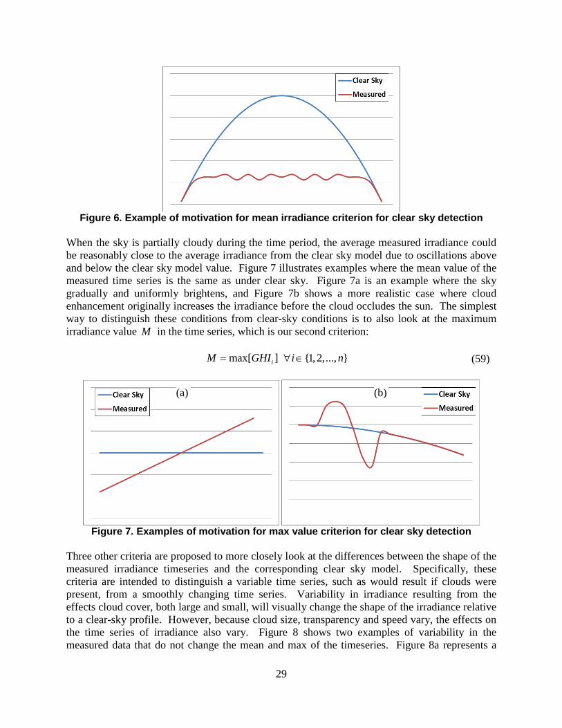
As illustrated in Figure 6, the mean irradiance G will be significantly lower if the sky is cloudy than under a clear sky.

29

Figure 6. Example of motivation for mean irradiance criterion for clear sky detection

When the sky is partially cloudy during the time period, the average measured irradiance could be reasonably close to the average irradiance from the clear sky model due to oscillations above and below the clear sky model value. Figure 7 illustrates examples where the mean value of the measured time series is the same as under clear sky. Figure 7a is an example where the sky gradually and uniformly brightens, and Figure 7b shows a more realistic case where cloud enhancement originally increases the irradiance before the cloud occludes the sun. The simplest way to distinguish these conditions from clear-sky conditions is to also look at the maximum irradiance value M in the time series, which is our second criterion:

max[ ] {1,2,..., }iM GHI i n= ∀ ∈ (59)

Figure 7. Examples of motivation for max value criterion for clear sky detection

Three other criteria are proposed to more closely look at the differences between the shape of the measured irradiance timeseries and the corresponding clear sky model. Specifically, these criteria are intended to distinguish a variable time series, such as would result if clouds were present, from a smoothly changing time series. Variability in irradiance resulting from the effects cloud cover, both large and small, will visually change the shape of the irradiance relative to a clear-sky profile. However, because cloud size, transparency and speed vary, the effects on the time series of irradiance also vary. Figure 8 shows two examples of variability in the measured data that do not change the mean and max of the timeseries. Figure 8a represents a

(a) (b)

30

small thick cumulous cloud, and Figure 8b represents high wispy cirrus clouds. The third, fourth and fifth criteria quantify aspects of variability in order to detect variability resulting from different types of clouds. The third proposed criterion measures variability in irradiance by the length L of the line connecting the points in the timeseries (Eq. 60). Any variability in the measured irradiance will increase the length of the line and be detected. .

( ) ( )2 2

1 11

n

i i i ii

L GHI GHI t t+ +=

= − + −∑ (60)

Figure 8. Examples of motivation for line length criterion for clear sky detection

However, the line length for a time series with a few, large changes, or with many small changes, may be similar to that of a smooth curve, necessitating additional criteria. The fourth criterion is the variance of changes in the time series; specifically, the normalized standard deviation σ of the slope (x) between sequential points in the series. While this criterion cannot easily detect situations such as Figure 8b if the slope between measurements varies slightly, Figure 9 shows a scenario where the line lengths are the same, but the variance of slope criterion (i.e., the fourth criterion) will easily distinguish between clear and cloudy periods with these features.

},...,2,1{ ,1 niGHIGHIs iii ∈∀−= + (61)

∑−

=−=

1

111 n

iix

ns

(62)

( )

∑

∑

=

−

=

−−= n

ii

n

ii

GHIn

ssn

1

1

1

2

11

1

σ

(63)

where iGHI indicates the measured GHI.

(a) (b)

31

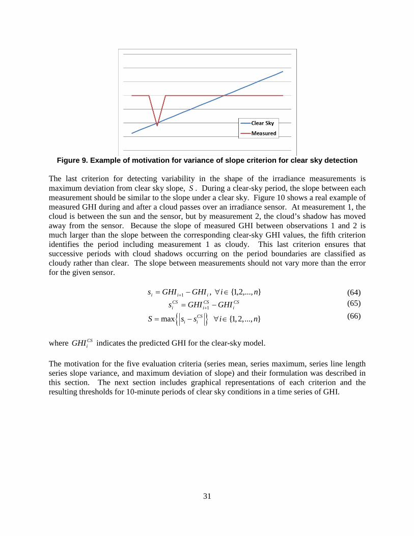
Figure 9. Example of motivation for variance of slope criterion for clear sky detection

The last criterion for detecting variability in the shape of the irradiance measurements is maximum deviation from clear sky slope, S . During a clear-sky period, the slope between each measurement should be similar to the slope under a clear sky. Figure 10 shows a real example of measured GHI during and after a cloud passes over an irradiance sensor. At measurement 1, the cloud is between the sun and the sensor, but by measurement 2, the cloud’s shadow has moved away from the sensor. Because the slope of measured GHI between observations 1 and 2 is much larger than the slope between the corresponding clear-sky GHI values, the fifth criterion identifies the period including measurement 1 as cloudy. This last criterion ensures that successive periods with cloud shadows occurring on the period boundaries are classified as cloudy rather than clear. The slope between measurements should not vary more than the error for the given sensor.

},...,2,1{ ,1 niGHIGHIs iii ∈∀−= + (64) CS

iCSi

CSi GHIGHIs −= +1 (65)

{ }max {1,2,..., }CSi iS s s i n= − ∀ ∈ (66)

where CS

iGHI indicates the predicted GHI for the clear-sky model. The motivation for the five evaluation criteria (series mean, series maximum, series line length series slope variance, and maximum deviation of slope) and their formulation was described in this section. The next section includes graphical representations of each criterion and the resulting thresholds for 10-minute periods of clear sky conditions in a time series of GHI.

32

Irrad

ianc

e (W

/m2 )

0 2 4 6 8 10Sequence of Measurements

Measured IrradianceClear Sky Irradiance

Figure 10. Example of motivation for maximum deviation from clear sky slope criterion

3.2.2. Moving Window Method for Classifying Individual Measurements. In Section 3.2, we described a method to identify periods of time with clear-sky conditions by examining the overall shape of the GHI vs. time curve. Here, we show how the method may be used to determine whether the sky is clear or cloudy for individual GHI measurements. Identifying periods of time as clear does not work well if there is any intermittent shading throughout the day such as a building, a pole, or power lines because the entire period would be declared as cloudy. For example, an hour of clear data would be thrown out because of a power line that blocked the sun for a minute during the hour, or a day would be classified as cloudy because of a building that blocks the sun in the morning for part of the year. One way to apply the method is by using a 10-minute moving window. The clear-sky criteria are evaluated for each 10-minute window, but each irradiance measurement is actually evaluated 10 times as the window moves through time (assuming the data has a 1 minute time step). The measured data in the moving window are compared to the clear sky model data for that window. Windows with acceptable criteria are flagged as clear. If an individual measurement is within at least one window declared as clear during the evaluations, the measurement is identified as clear. Another way to think about it is that the window checks every combination of adjacent 10 measurements, and if at least one combination meets the five detection criteria, then all 10 measurements in that window must be clear. This method allows each measurement to be classified as clear or cloudy. Measured GHI data from the Clark Station MIDC site in Las Vegas, Nevada, which are subject to intermittent shading by power lines and poles, illustrate the potential application of this method. Figure 11 shows the satellite image showing the power lines near the irradiance sensor at the MIDC site Clark Station in Las Vegas, Nevada. Shadows from the power lines show in the irradiance profile in Figure 12 in the morning and evening as the sun crosses the lines. At certain times of year the path of the sun crosses one of the poles, so the direct component of the irradiance is zero every evening; an example is shown in Figure 13.

33

Figure 11. Satellite Image of Clark Station, NV

7.336 7.336 7.336 7.336 7.336 7.336

x 105

0

100

200

300

400

500

600

700

800

900

1000

Time

GH

I (W

/m2 )

Measured GHIClear Sky

Figure 12. Measured GHI at Clark Station showing effect of power lines

34

7.3306 7.3306 7.3306 7.3306 7.3306 7.3306 7.3306 7.3306 7.3306

x 105

0

100

200

300

400

500

600

Time

GH

I (W

/m2 )

Measured GHIClear Times

Figure 13. Measured GHI at Clark Station showing effect of a pole

3.2.3. Threshold Values for Criteria In order to apply the algorithm, a threshold value must be established for each criterion. Below are the criteria and example results using a 10-minute moving time window. If a different length time period was chosen, the thresholds for each criterion would need to be adjusted. A simple fixed tolerance threshold is in place for the series mean and maximum criteria. Most evaluations of clear sky models find that the average bias error of the model is less than 10%, often around 7% [1, 83]. Therefore, a fixed threshold of ±75 W/m2 within the mean and max of the clear sky model was chosen. To determine threshold values for other criteria, we examined recorded GHI at Fort Apache station in Las Vegas, NV. We manually identified clear-sky periods by the shape of the GHI vs. time curve and its magnitude compared to a simple clear-sky model. We then calculated values for each criterion for both clear and cloudy periods, then selected thresholds that would distinguish between conditions. The calculated line length for the 10-minute moving window on a clear day is shown in Figure 14. Using the data shown in Figure 14 and data for other clear days (not shown), thresholds of within +10 and -5 of the clear sky line length were chosen. Figure 15 shows how clearly the line length increases with variability from cloud cover. Figure 16 shows that on a clear day the variance of slopes between GHI measurements in the 10-minute moving window are consistently flat throughout the day. Based on this data, a fixed value of 0.005 is chosen as the threshold for the variance of slope criterion. Under cloudy conditions as shown in Figure 17, the slope variance clearly exceeds the threshold.

35

6 8 10 12 14 16 18

101

102

Time of Day

Line

Len

gth

May 5, 2011

6 8 10 12 14 16 180

200

400

600

800

1000

1200

Irrad

ianc

e (W

/m2 )

Clear Sky Line LengthMeasured Line LengthClear Sky IrradianceMeasured Irradiance

Figure 14. Line length of GHI in a 10-minute moving window on a clear day

6 8 10 12 14 16 18

101

102

Time of Day

Line

Len

gth

May 8, 2011

6 8 10 12 14 16 180

200

400

600

800

1000

1200

Irrad

ianc

e (W

/m2 )

Clear Sky Line LengthMeasured Line LengthClear Sky IrradianceMeasured Irradiance

Figure 15. Line length of GHI in a 10-minute moving window on a cloudy day

The last threshold is for the maximum deviation from average clear sky slope. The measured irradiance data is from real sensors with a certain noisy measurement error. For most GHI sensors, both thermopiles and silicon-based sensors, the sensor error is about 5% and at best it is 2% [100, 101]. An uncorrected precision spectral pyranometer (PSP) is a notable exception to this rule. Assuming a 4% possible error on the sensor, this means the maximum deviation in slope due to sensor error is 8%, so a difference of 8 W/m2 per time period between measured and modeled irradiance change is chosen as the threshold.

36

6 8 10 12 14 16 180

0.01

0.02

0.03

0.04

0.05

0.06

Time of Day

Varia

nce

May 5, 2011

6 8 10 12 14 16 180

200

400

600

800

1000

1200

Irrad

ianc

e (W

/m2 )

Measured VarianceClear Sky IrradianceMeasured Irradiance

Figure 16. Variance of the slopes of GHI in a 10-minute moving window on a clear day

6 8 10 12 14 16 180

0.01

0.02

0.03

0.04

0.05

0.06

Time of Day

Varia

nce

May 8, 2011

6 8 10 12 14 16 180

200

400

600

800

1000

1200

Irrad

ianc

e (W

/m2 )

Measured VarianceClear Sky IrradianceMeasured Irradiance

Figure 17. Variance of slopes of GHI in a 10-minute moving window on a cloudy day

3.3. Iterative Process for Improved Detection of Clear Days It is important to note that detection of clear times depends on the clear-sky model to which the measured data are compared. Poorly calibrated sensors that report systematically low readings, or choice of an inaccurate clear sky model with a large bias, could cause clear periods to be misidentified as cloudy, by failing to meet the criteria for mean or maximum irradiance. Manual identification of clear sky times is very tedious for the large amount of data, but the automated method requires comparing the shape of measured irradiance to a clear sky model. To address

37

this problem, we propose an iterative method to adjust for differences between the clear sky model and sensor data. The proposed method is an iterative process where clear days are detected, a clear sky model is fit to the clear measurements, and then more clear days are detected from the improved clear sky model. The process is iterated until no more clear periods are detected. The iterative method is shown in Figure 18. Section 4 shows that the largest error between clear sky models and measured data for a location is scaling factor to correct for any sensor calibration issues or clear sky model constants like altitude. This means that the shape of the clear sky model is similar to measured data times a scaling coefficient (α). The iterative process solves for α by minimizing RMSE between measured (GHI) and clear sky irradiance (CSI) (Eq. (67)), using an optimization method such as the Nelder-Mead simplex method. The method from Section 3.2 is used to identify clear times, and only clear times on days where greater than 50% of the day is clear are used to calibrate the clear sky detection algorithm in the optimization problem. Basically, a few clear days are first detected and data from these days are used to improve the clear sky model. This continues until α has converged and no new clear days are being identified.

Run Clear Sky Model

Detect Clear Times

Modify Clear Sky

Model

Converged?Fit Model to Clear Times

No

Yes

Figure 18. Flow chart for adaptive clear time detection algorithm

( )2

1( )

Minimize

subject to >0

n

i ii

GHI CSIf

n

αα

α

=

× −=∑

(67)

3.4. Visual Verification of Clear Sky Detection While it is difficult to fully verify the accuracy of our proposed method for automating detection of clear and cloudy periods, a visual confirmation of the detection algorithm is shown in Figure 19 and Figure 20. These graphs show the measured irradiance along with the red markers for if each minute is detected as clear.

38

5 10 150

500

1000

01-Apr-2007

Hour

Irrad

ianc

e (W

/m2 )

5 10 150

500

1000

02-Apr-2007

Hour

Irrad

ianc

e (W

/m2 )

5 10 150

500

1000

03-Apr-2007

Hour

Irrad

ianc

e (W

/m2 )

5 10 150

500

1000

04-Apr-2007

Hour

Irrad

ianc

e (W

/m2 )

5 10 150

500

1000

05-Apr-2007

Hour

Irrad

ianc

e (W

/m2 )

5 10 150

500

1000

06-Apr-2007

Hour

Irrad

ianc

e (W

/m2 )

5 10 150

500

1000

07-Apr-2007

Hour

Irrad

ianc

e (W

/m2 )

5 10 150

500

1000

08-Apr-2007

Hour

Irrad

ianc

e (W

/m2 )

5 10 150

500

1000

09-Apr-2007

Hour

Irrad

ianc

e (W

/m2 )

5 10 150

500

1000

10-Apr-2007

Hour

Irrad

ianc

e (W

/m2 )

5 10 150

500

1000

11-Apr-2007

Hour

Irrad

ianc

e (W

/m2 )

5 10 150

500

1000

12-Apr-2007

Hour

Irrad

ianc

e (W

/m2 )

5 10 150

500

1000

13-Apr-2007

Hour

Irrad

ianc

e (W

/m2 )

5 10 150

500

1000

14-Apr-2007

Hour

Irrad

ianc

e (W

/m2 )

5 10 150

500

1000

15-Apr-2007

Hour

Irrad

ianc

e (W

/m2 )

Figure 19. Visual representation of clear sky detection. Measured irradiance is in blue, with red markers signifying minutes identified as clear.

39

5 10 150

500

1000

16-Apr-2007

Hour

Irrad

ianc

e (W

/m2 )

5 10 150

500

1000

17-Apr-2007

Hour

Irrad

ianc

e (W

/m2 )

5 10 150

500

1000

18-Apr-2007

Hour

Irrad

ianc

e (W

/m2 )

5 10 150

500

1000

19-Apr-2007

Hour

Irrad

ianc

e (W

/m2 )

5 10 150

500

1000

20-Apr-2007

Hour

Irrad

ianc

e (W

/m2 )

5 10 150

500

1000

21-Apr-2007

Hour

Irrad

ianc

e (W

/m2 )

5 10 150

500

1000

22-Apr-2007

Hour

Irrad

ianc

e (W

/m2 )

5 10 150

500

1000

23-Apr-2007

Hour

Irrad

ianc

e (W

/m2 )

5 10 150

500

1000

24-Apr-2007

Hour

Irrad

ianc

e (W

/m2 )

5 10 150

500

1000

25-Apr-2007

Hour

Irrad

ianc

e (W

/m2 )

5 10 150

500

1000

26-Apr-2007

Hour

Irrad

ianc

e (W

/m2 )

5 10 150

500

1000

27-Apr-2007

Hour

Irrad

ianc

e (W

/m2 )

5 10 150

500

1000

28-Apr-2007

Hour

Irrad

ianc

e (W

/m2 )

5 10 150

500

1000

29-Apr-2007

Hour

Irrad

ianc

e (W

/m2 )

5 10 150

500

1000

30-Apr-2007

Hour

Irrad

ianc

e (W

/m2 )

Figure 20. Visual representation of clear sky detection. Measured irradiance is in blue, with red markers signifying instants identified as clear.

40

41

4. ANALYSIS OF CLEAR SKY MODELS

The clear sky models are compared to measured clear sky data from 30 different locations to test their accuracy and each model’s sensitivity to location and time dependence. The evaluation criteria are described in Section 4.1. In Section 4.2, we describe the irradiance data to which models are compared and the thresholds used to identify clear-sky periods. Analysis of model performance is presented in Section 4.3. 4.1. Evaluation Criteria Model errors are analyzed using two key statistical criteria: Root Mean Square Error (RMSE), and Mean Bias Error (MBE). RMSE demonstrates the general overall accuracy of the model, while MBE shows if the model is generally high or low.

( )( )( )ImeasuredGHmean

ImeasuredGHdelclearSkyMomeanRMSE

2−= (68)

( )

( )ImeasuredGHmeanImeasuredGHdelclearSkyMomeanMBE −

= (69)

We quantified model performance using these two metrics for a set of clear days determined from irradiance measurements at a number of sites in the United States. We also examined how these error metrics depend on common model inputs, including: zenith angle; time of day; time of year; location; and elevation. 4.2. Irradiance data The measured GHI data used in the clear sky model analysis is from the 30 sites shown in Figure 21. The data was obtained from NREL’s Measurement and Instrumentation Data Center (MIDC) [102], NOAA’s Surface Radiation (SURFRAD) Network [103], and the Las Vegas Valley Water District’s installed PV plant locations. In total, about 300 years of data were used in the analysis. Of this data, about 12,000 days were detected as clear days using the method described in Section 3. The site names, locations, time of measured data used, and number of clear days detected are shown in Table 2.

42

Figure 21. Measurement sites used in the analysis

Table 2. Table of irradiance measurement sites and number of detected clear days

Site Name Latitude Longitude Altitude Start Time End Time Clear Days Albuquerque, NM 35.04 -106.62 1617 2/1/2002 10/31/2011 765 Bismarck, ND 46.77 -100.77 503 2/1/2002 10/31/2011 206 Bondville, IL 40.05 -88.37 213 1/1/1995 10/31/2011 447 Desert Rock, NV 36.624 -116.019 1007 3/16/1998 10/31/2011 1691 Fort Peck, MT 48.31 -105.1 634 1/28/1995 10/31/2011 443 Goodwin Creek, Batesville, MS 34.25 -89.87 98 1/1/1995 10/31/2011 652 Hanford, CA 36.31 -119.63 73 2/1/2002 10/31/2011 415 Madison, WI 43.13 -89.33 271 2/1/2002 10/31/2011 282 Penn State, Ramblewood, PA 40.72 -77.93 376 6/29/1998 10/31/2011 192 Salt Lake City, UT 40.77 -111.97 1288 2/1/2002 10/31/2011 681 Seattle, WA 47.68 -122.25 20 2/1/2002 10/31/2011 241 Sioux Falls, SD 43.73 -96.62 473 6/15/2003 10/31/2011 286 Sterling, VA 38.98 -77.47 85 2/2/2002 10/31/2011 221 Table Mountain, Boulder, CO 40.13 -105.24 1689 8/1/1995 10/31/2011 559 Anatolia, Rancho Cordova, CA 38.54586 -121.2403 51 2/4/2009 6/30/2011 195 Bluefield, WV 37.27 -81.24 803 11/6/1985 11/1/2011 335 Elizabeth City, NC 36.28 -76.22 26 9/25/1985 11/1/2011 679 Las Vegas, NV (Fort Apache) 36.2205 -115.296 774 8/23/2006 4/30/2009 340 Las Vegas, NV (Grand Canyon) 36.2204 -115.307 807 9/30/2006 4/30/2009 291 Lowry Range, East Arapahoe, CO 39.60701 -104.5802 1860 6/1/2008 10/26/2011 130 Las Vegas, NV (Luce) 36.201 -115.262 738 5/2/2007 4/30/2009 229 Las Vegas, NV (LVSP) 36.172 -115.191 661 7/26/2007 4/30/2009 207

43

NWTC, Boulder, CO 39.91065 -105.2348 1855 8/24/2001 11/1/2011 236 NREL, Golden, CO (a) 39.74 -105.18 1829 1/1/2004 6/30/2011 231 Oak Ridge, TN 35.92996 -84.30952 245 2/2/2002 10/26/2011 185 Las Vegas, NV (Ronzone) 36.193 -115.234 705 4/27/2006 4/30/2009 341 Sandia Labs, Albuquerque, NM 35.0545 -106.5401 1658 6/28/2001 6/14/2011 584 South Park, Pike Forest, CO 39.27278 -105.6247 2944 3/29/1997 11/1/2011 150 Las Vegas, NV (Spring Mountain) 36.125 -115.285 805 11/30/2006 4/30/2009 312 UNLV, Las Vegas, NV 36.06 -115.08 615 1/1/2007 12/31/2011 389

(a) Only site used to evaluate the REST2 model As shown in Table 2, only clear days were used in the analysis. To determine the set of clear days, we used the algorithm presented in Section 3 and selected only days where the 90% of the day is clear. 4.3. Model Analysis 4.3.1. Models Under Consideration In our analysis of clear-sky models, we considered the following models:

− Adnot–Bourges–Campana–Gicquel (ABCG) model (Eq. 20; [1]); − Berger–Duffie (BD) model (Eq. 19; [1]); − Daneshyar–Paltridge–Proctor (DPP) model (Eq. 14, 15, 16; [12, 13]); − Haurwitz model (Eq. 18; [15, 16]); − Kasten–Czeplak (KC) model (Eq. 17; [14]); − Robledo-Soler (RS) (Eq. 21; [17]); − Ineichen (Sect. 2.4; [21]); − Atwater and Ball (Sect. 2.5; [26, 27]); − REST2 (Sect. 2.5; [29, 35, 36]).

Due to the number of atmospheric input parameters required for the REST2 model, this model is only implemented for the Solar Radiation Research Laboratory (SRRL) site at NREL in Golden, CO. As documented by NREL, aerosol optical depth is determined from on-site readings from a Kipp & Zonen pyrheliometer. Albedo is measured on-site from an inverted LI-200 at 2 meters above the ground. Reduced ozone vertical pathlength measurements are available from either an on-site measurements before 2005 or from Ozone Monitoring Instrument (OMI) satellite. Angstrom’s turbidity coefficient is measured on-site by a 500nm photometer. Precipitable water is measured on-site using a 7-channel photometer. Station pressure is measured on-site by a Vaisala pressure transmitter. Default values are used for Angstrom’s wavelength exponents, aerosol single-scattering albedo, and reduced NO2 vertical pathlength. 4.3.2. Average Model Error Figure 22 shows the RMSE and MBE for each model averaged over all sites (a single site in the case of the REST2 model). The lowest RMSE is achieved by REST2 with 4.7%. The Ineichen model is not far behind with an RMSE of 5.0%. Some of the very simple clear sky models

44

perform very poorly, such as KC, but the Haurwitz model has a 6.6% RMSE. The lowest MBE is Atwater with -0.3%. As indicated by the negative values for MBE, on average all of the models under-predict the amount of GHI. Note that for some models, like ABCG and KC, the error is coming from a large bias error between the measured and predicted. On the other hand, models like Haurwitz and Atwater have very small bias errors.

ABCG BD DPP Haurwitz KC RS Ineichen Atwater REST2-0.15

-0.1

-0.05

0

0.05

0.1

0.15

0.2

Average RMSEAverage MBE

Figure 22. Average RMSE and MBE as a percentage of measured irradiance for each

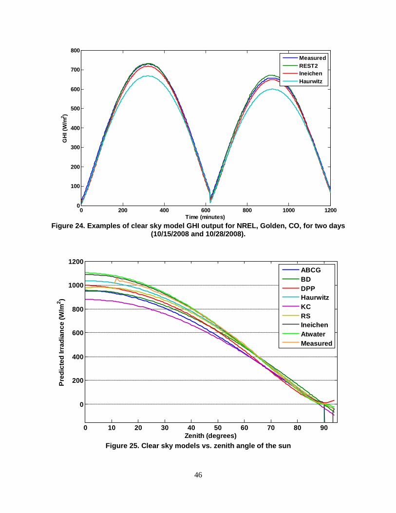
clear sky model at all sites The under-prediction bias of the models can be seen in Figure 22 where the clear sky model predictions are plotted against the measured values. Each model has a similar spread or width of the data, but the angle of some models is significantly off. From this it appears that a simple multiplication factor could be applied to these models to bring them closer to the measured GHI. The outliers in the REST2 model results are most likely due to errors in the measured atmospheric measurements. 4.3.3. Dependence of Model Error on Zenith Angle Every model uses the zenith angle of the sun as an input, so each model’s output GHI will have a similar shape, height, and width due to the position of the sun. Measured GHI at NREL, Golden, CO for two example clear days are shown in Figure 24 along with the results of three clear-sky models: a complex model, REST2; a simple model, the Ineichen model; and a very simple model by Haurwitz. Note that all very simple clear sky models tend to significantly underpredict the irradiance for Golden, CO, and other high altitude locations because site elevation is not an input. In Section 4.3.6 we examine the relationship between site elevation and model error.

45

Figure 23. Measured GHI vs. predicted GHI for each clear sky model

In Figure 3 the very simple clear sky models were plotted as a function of zenith angle. More complicated models like the Ineichen model, which have inputs other than zenith angle, can yield a range of output for a given zenith angle. To plot these models and measured irradiance as a function of zenith angle we first binned model output and measured irradiance by zenith angle using bins of 0.01 radians in width, then averaged the values within each bin. The results are plotted in Figure 25. The graph shows how the various clear-sky models compare to average measured GHI as a function of zenith angle.

46

0 200 400 600 800 1000 12000

100

200

300

400

500

600

700

800

Time (minutes)

GH

I (W

/m2 )

MeasuredREST2IneichenHaurwitz

Figure 24. Examples of clear sky model GHI output for NREL, Golden, CO, for two days

(10/15/2008 and 10/28/2008).

0 10 20 30 40 50 60 70 80 90

0

200

400

600

800

1000

1200

Zenith (degrees)

Pred

icte

d Irr

adia

nce

(W/m

2 )

ABCGBDDPPHaurwitzKCRSIneichenAtwaterMeasured

Figure 25. Clear sky models vs. zenith angle of the sun

47

The dependence of model error (predicted GHI – measured GHI) on zenith angle can be more clearly seen in Figure 26 where the difference between the modeled and average measured GHI are plotted for each model. It is interesting to note that at zenith angle between 15 and 60 degrees, the error appears to change linearly in zenith angle for each model.

0 10 20 30 40 50 60 70 80 90-150

-100

-50

0

50

100

Zenith (degrees)

Diff

eren

ce fr

om M

easu

red

Irrad

ianc

e (W

/m2 )

ABCGBDDPPHaurwitzKCRSIneichenAtwater

Figure 26. Dependence of model error on zenith angle

4.3.4. Dependence of Model Error on Time of Day and Time of Year It is also interesting to investigate the dependence of the error of each model on the time of day and the season of the year. The time varying errors are all analyzed looking at the difference in GHI (W/m2) between the modeled and measured. We calculated the model error for each hour of each day, and then averaged within the same hour, over all days and sites; Figure 27 shows the results for each model. Showing these bias errors throughout the day assists in understanding the average RMSE and average bias errors for each model, and shows why the ABCG and KC models have a large bias error and the Ineichen and Atwater models have very low average bias. Because Figure 27 shows bias error averaged within each hour over all days and sites, there is an amount of uncertainty to each line. Figure 28 shows error bars representing the standard deviation of the bias values during each hour. This gives a feel for the range of bias values that occur for each model for each time period.

48

5 6 7 8 9 10 11 12 13 14 15 16 17 18 19-160

-140

-120

-100

-80

-60

-40

-20

0

20

40

Time of Day

Mea

n Er

ror (

W/m

2 )

ABCGBDDPPHaurwitzKCRSIneichenAtwaterREST2

Figure 27. Average error for each clear sky model by time of day

49

6 8 10 12 14 16 18

-150

-100

-50

0

50

ABCG

Time of Day

Mea

n Er

ror (

W/m

2 )

6 8 10 12 14 16 18

-150

-100

-50

0

50

BD

Time of DayM

ean

Erro

r (W

/m2 )

6 8 10 12 14 16 18

-150

-100

-50

0

50

DPP

Time of Day

Mea

n Er

ror (

W/m

2 )

6 8 10 12 14 16 18

-150

-100

-50

0

50

Haurwitz

Time of Day

Mea

n Er

ror (

W/m

2 )

6 8 10 12 14 16 18

-150

-100

-50

0

50

KC

Time of Day

Mea

n Er

ror (

W/m

2 )

6 8 10 12 14 16 18

-150

-100

-50

0

50

RS

Time of DayM

ean

Erro

r (W

/m2 )

6 8 10 12 14 16 18

-150

-100

-50

0

50

Ineichen

Time of Day

Mea

n Er

ror (

W/m

2 )

6 8 10 12 14 16 18

-150

-100

-50

0

50

Atwater

Time of Day

Mea

n Er

ror (

W/m

2 )

6 8 10 12 14 16 18

-150

-100

-50

0

50

REST2

Time of Day

Mea

n Er

ror (

W/m

2 )

Figure 28. Average error for each clear sky model by time of day, with error bars

50

The same analysis that was done for time of day can be done for the day of the year, to investigate seasonal variations in model error. We averaged model error by month over all sites and show the results in Figure 29. For most models, a characteristic shape is observed, with the average error reaching a minimum in the spring and a maximum in the summer. The REST2 model does not follow this trend. The general bias toward underestimating GHI is also evident for most models. For several models with low MBE (i.e., Atwater, Haurwitz, and RS), we can observe that the low MBE results by averaging underestimates of GHI in the spring with overestimates in the summer. The general shape of the curves could be attributed to the temperature dependence of the reference ground sensors. Pyranometers have a temperature dependence that would measure higher GHI (by a few percent) when it is cooler in March and lower GHI during the hot season in August. Advanced instrument calibration procedures can account for these effects.

1 2 3 4 5 6 7 8 9 10 11 12-120

-100

-80

-60

-40

-20

0

20

Month

Mea

n Er

ror (

W/m

2 )

ABCGBDDPPHaurwitzKCRSIneichenAtwaterREST2

Figure 29. Average monthly error for each clear sky model throughout the year

The standard deviation for each model’s average monthly error is shown in Figure 30.

51

1 2 3 4 5 6 7 8 9 101112

-150

-100

-50

0

50

ABCG

Month

Mea

n Er

ror (

W/m

2 )

1 2 3 4 5 6 7 8 9 101112

-150

-100

-50

0

50

BD

Month

Mea

n Er

ror (

W/m

2 )

1 2 3 4 5 6 7 8 9 101112

-150

-100

-50

0

50

DPP

Month

Mea

n Er

ror (

W/m

2 )

1 2 3 4 5 6 7 8 9 101112

-150

-100

-50

0

50

Haurwitz

Month

Mea

n Er

ror (

W/m

2 )

1 2 3 4 5 6 7 8 9 101112

-150

-100

-50

0

50

KC

Month

Mea

n Er

ror (

W/m

2 )

1 2 3 4 5 6 7 8 9 101112

-150

-100

-50

0

50

RS

Month

Mea

n Er

ror (

W/m

2 )

1 2 3 4 5 6 7 8 9 101112

-150

-100

-50

0

50

Ineichen

Month

Mea

n Er

ror (

W/m

2 )

1 2 3 4 5 6 7 8 9 101112

-150

-100

-50

0

50

Atwater

Month

Mea

n Er

ror (

W/m

2 )

1 2 3 4 5 6 7 8 9 101112

-150

-100

-50

0

50

REST2

Month

Mea

n Er

ror (

W/m

2 )

Figure 30. Average monthly error for each clear sky model throughout the year with error

bars The model error can be plotted for both the time of day and day of the year in a contour plot shown in Figure 31. If the measured irradiance was solely a function of zenith angle, then the model errors would also be a function of zenith angle. For example, a certain zenith angle would have the same error whenever it occurred during the year. This would reveal very distinct circles with concentric symmetry in the center of the figures in Figure 31. The absence of such patterns shows that dependence on other parameters other than zenith angle should be considered to improve accuracy of a clear-sky model. The error shown for the REST2 model appears to be generally uniform for all times and days; however, this error is quantified only at the single site where the REST2 model was applied, whereas the error for other models is averaged over many sites.

52

Mean Error (W/m2) for ABCG

Month

Tim

e of

Day

2 4 6 8 10 126

8

10

12

14

16

18

-200

-150

-100

-50

0

Mean Error (W/m2) for BD

Month

Tim

e of

Day

2 4 6 8 10 126

8

10

12

14

16

18

-200

-150

-100

-50

0

Mean Error (W/m2) for DPP

Month

Tim

e of

Day

2 4 6 8 10 126

8

10

12

14

16

18

-200

-150

-100

-50

0

Mean Error (W/m2) for Haurwitz

Month

Tim

e of

Day

2 4 6 8 10 126

8

10

12

14

16

18

-200

-150

-100

-50

0

Mean Error (W/m2) for KC

Month

Tim

e of

Day

2 4 6 8 10 126

8

10

12

14

16

18

-200

-150

-100

-50

0

Mean Error (W/m2) for RS

Month

Tim

e of

Day

2 4 6 8 10 126

8

10

12

14

16

18

-200

-150

-100

-50

0

Mean Error (W/m2) for Ineichen

Month

Tim

e of

Day

2 4 6 8 10 126

8

10

12

14

16

18

-200

-150

-100

-50

0

Mean Error (W/m2) for Atwater

Month

Tim

e of

Day

2 4 6 8 10 126

8

10

12

14

16

18

-200

-150

-100

-50

0

Mean Error (W/m2) for REST2

Month

Tim

e of

Day

2 4 6 8 10 126

8

10

12

14

16

18

-200

-150

-100

-50

0

Figure 31. Average error (W/m2) for each clear sky model for each hour and month

4.3.5. Dependence of Model Error on Location We examined the dependence of model error on site location by computing the RMSE at each location for each model. Figure 32 shows the RMSE for each model, drawing a curve for each location to show how error at one location relates across models. This plot shows that, in general, GHI is more difficult to predict at some sites than at others, regardless of the model used. For example, the RMSE at South Park, Pike National Forest, CO, (the uppermost curve), tends to be greater than at any other site for most clear-sky models. No range is shown for the REST2 model because it was applied at only a single location. The variation in model error across sites is largely due to site elevation as we show in Section 4.3.6. Figure 33 summarizes the range of RMSE that are observed for each model, across all sites listed in Table 2. The box encloses the 25th to 75th percentile range; the red bar indicates the median value of RMSE; and the tails of each whisker show the extremes.

53

ABCG BD DPP Haurwitz KC RS Ineichen Atwater REST2

0.05

0.1

0.15

0.2

0.25

0.3

RM

SE

Albuquerque Bismarck Bondville Desert Rock Fort Peck Goodwin Creek Hanford Madison Penn State Salt Lake City Seattle Sioux Falls Sterling Table MountainAnatoliaBluefieldElizabethCityFort ApacheGrand CanyonLowryRangeLuceLVSPNationalWindTechCenterNRELOakRidgeRonzoneSandiaSouthParkSpring MountainUNLV

Figure 32. RMSE for each site and each clear sky model

Figure 34 plots RMSE by location, drawing one curve for each clear sky model. This figure shows that a model with large errors at one site is also likely to have large errors at other sites, and conversely, more accurate models tend to be more accurate at each site, and that the overall accuracy of a clear-sky model is generally summarized by the average error over many sites. However, model accuracy depends fairly strongly on site elevation, with very simple models being less accurate at higher elevations (Section 4.3.6). Focusing on the results for two locations, Figure 35 shows the RMSE and MBE for Albuquerque and Figure 36 shows the RMSE and MBE for Las Vegas. Greater RSME is shown for Albuquerque, NM, than for Las Vegas, NV, for every model other than the Ineichen model. In addition, MBE is generally greater in magnitude for Albuquerque, NM, than for Las Vegas, NV, for all other models except KC.

54

0.04

0.06

0.08

0.1

0.12

0.14

0.16

0.18

0.2

0.22

0.24

ABCG BD DPP Haurwitz KC RS Ineichen Atwater REST2

RM

SE

Figure 33. RMSE for clear sky models

0

0.05

0.1

0.15

0.2

0.25

Alb

uque

rque

Bis

mar

ck B

ondv

ille

Des

ert R

ock

For

t Pec

k G

oodw

in C

reek

Han

ford

Mad

ison

Pen

n St

ate

Sal

t Lak

e C

ity S

eattl

e S

ioux

Fal

ls S

terli

ng T

able

Mou

ntai

nA

nato

liaB

luef

ield

Eliz

abet

hCity

Fort

Apa

che

Gra

nd C

anyo

nLo

wry

Ran

geLu

ceLV

SPW

indT

echC

ente

rN

REL

Oak

Rid

geR

onzo

neSa

ndia

Sout

hPar

kSp

ring

Mou

ntai

nU

NLV

RM

SE

ABCG BD DPP Haurwitz KC RS Ineichen Atwater

Figure 34. Range of RMSE at each site for clear sky models

55

ABCG BD DPP Haurwitz KC RS Ineichen Atwater-0.2

-0.15

-0.1

-0.05

0

0.05

0.1

0.15

0.2

0.25

RMSEMBE

Figure 35. Results for eight clear sky models in Albuquerque, NM

ABCG BD DPP Haurwitz KC RS Ineichen Atwater-0.15

-0.1

-0.05

0

0.05

0.1

0.15

0.2

RMSEMBE

Figure 36. Results for eight clear sky models for Fort Apache station in Las Vegas, NV

4.3.6. Dependence of Model Error on Elevation From Section 4.3.5, a variation in clear sky model errors can be seen between sites. The clear sky irradiance on the ground is a function of the site altitude, so very simple models that do not adjust for altitude may decrease in accuracy at higher elevations. Figure 37 shows how the very simple clear sky models significantly underpredict irradiance as the elevation increases. The MBE for each of the six very simple clear sky models considered in this report (ABCG, BD, DPP, Haurwitz, KC, and RS) was averaged at each site location to produce the errors represented

56

for the very simple models in Figure 37. The Ineichen model does have a correction term for site elevation, so model error depends only weakly on elevation. As shown in Figure 38, the RMSE error is also dependent on site elevation. The Ineichen model that accounts for altitude shows almost no dependence on site elevation, but higher elevations introduce significant error in the very simple clear sky models.

Figure 37. Dependence of model error (MBE) on site elevation

Figure 38. Dependence of model error (RMSE) on site elevation

57

5. CONCLUSIONS

A wide range of models for global horizontal irradiance during clear skies were studied. Among these models, it was found that the complex models, specifically, the REST2 and Ineichen models, which account for many of the atmospheric parameters are most accurate. When model error is averaged over many locations and days, the REST2 model performed best with an RMSE of 4.7%; however, we were able to evaluate the REST2 model’s accuracy at only a single location due to its need for site specific data that are rarely available at most locations. Several other authors have found REST2 to be the most accurate model [86, 87]. Over many sites, the Ineichen model performed with accuracy similar to REST2 with an RMSE of 5.0%. Gueymard also found the Ineichen model to be comparable to REST2 [87]. The Ineichen model relies on a gridded dataset that varies by month and location, but the model does not need other site-specific data and is therefore quite easy to implement anywhere. Due to this ease of application and high degree of performance it is recommended for use in most locations, unless you have data available to use the REST2 model. However, the performance of several simple models was comparable; for example, the Haurwitz and Robledo-Soler models had RMSE of 6.6% and 7.3%, respectively. Other authors have also found that simple models are comparable in accuracy to more complicated models [1]. The development of a complex clear sky model for a location is a time consuming processing, and complex models are also heavily dependent on having local measurements [82]. Thus, for many applications simple clear-sky models may be suitable. Models with large errors at one site tended to also show large errors at other sites. For simple clear-sky models which do not account for altitude, we observed a significant dependence of model error on a site’s altitude. This conclusion suggests that simple clear-sky models may be suitable for lower elevations, but accurate modeling at higher elevations may require a more complex model. We also examined the relationship between model error and time of day, day of year, and zenith angle. More accurate models did not exhibit a strong dependence of model error on zenith angle. However, all simple clear-sky models showed a greater sensitivity of model error to time of day and day of year. These model errors vary in a complex fashion throughout the year (Figure 31). If analyses are confined to specific periods of time, the dependence of error on time of day and year may inform selection of a clear-sky model. We also compared models which support clear-sky models, namely, models that calculate solar position (Section 2.2), extraterrestrial radiation (Section 2.3) and air mass (Section 2.8). Zenith angle calculated using more simple approaches is generally within 0.4% of that determined by the best available method [9]. Simple methods for extraterrestrial radiation are also comparable to those given in [9]. Except at very high zenith angles (i.e., exceeding 85 degrees), all models we considered for air mass yield equivalent results. Choice of these models will depend on the accuracy desired in an individual analysis.

58

It is important to remember that the irradiance sensors also have a certain amount of error, generally in the range of 2% to 5% [100, 101] for well maintained and calibrated instruments, but sometimes greater. The analysis and evaluation in this study is performed by comparing the clear sky models to measurements with this innate inaccuracy. Clear sky models are also themselves essentially functions fit to measured data with error. Clear sky models have been shown to be able to predict global irradiance within the uncertainty of broadband measurements [87]. This observation suggests that clear sky models could be used to help detect and possibly correct problems with irradiance data collected from instruments that may not have been well-calibrated or maintained, by comparing measured data to predictions for clear days. For photovoltaic (PV) applications, historical GHI measurements are of great value in predicting the future energy production from proposed PV plants. Because a bias error in measured GHI would cause corresponding bias errors in energy, irradiance data for this application may be improved by understanding the bias errors in the measured data and how bias errors vary with other variables (e.g., zenith angle, altitude, etc.). If comparisons to clear sky models can help to validate and improve existing sources of GHI measurements (by identifying and reducing bias errors) then the value of these existing data sources can be enhanced.

59

60

6. REFERENCES

[1] V. Badescu, "Verification of some very simple clear and cloudy sky models to evaluate

global solar irradiance," Solar Energy, vol. 61, pp. 251-264, Oct 1997. [2] T. Stoffel, D. Renne, D. Myers, S. Wilcox, M. Sengupta, R. George, and C. Turchi,

"Concentrating Solar Power: Best Practices Handbook for the Collection and Use of Solar Resource Data (CSP)," NREL/TP-550-47465, 2010.

[3] J. A. Davies and D. C. McKay, "Evaluation of selected models for estimating solar radiation on horizontal surfaces," Solar Energy, vol. 43, pp. 153-168, 1989.

[4] C. A. Gueymard and D. R. Myers, "Solar Radiation Measurement: Progress in Radiometry for Improved Modeling," in Modeling Solar Radiation at the Earth’s Surface, V. Badescu, Ed., ed Heidelberg, Germany: Springer-Verlag Berlin Heidelberg, 2008.

[5] R. G. Allen, Environmental, and E. Water Resources institute . Task Committee on Standardization of Reference, The ASCE standardized reference evapotranspiration equation. Reston, Va.: American Society of Civil Engineers, 2005.

[6] J. W. Spencer, "Fourier series representation of the sun," Search, vol. 2, p. 172, 1971. [7] NREL. (February 2000). SOLPOS: Solar Position and Intensity. Available:

http://rredc.nrel.gov/solar/codesandalgorithms/solpos/ [8] NREL. (February 2000). SOLPOS Online Calculator. Available:

http://www.nrel.gov/midc/solpos/solpos.html [9] I. Reda and A. Andreas. (2003). "Solar Position Algorithm for Solar Radiation

Applications". NREL Report No. TP-560-34302. http://www.nrel.gov/docs/fy08osti/34302.pdf

[10] I. Reda and A. Andreas, "Solar position algorithm for solar radiation applications," Solar Energy, vol. 76, pp. 577-589, 2004.

[11] A. Ianetz and A. Kudish, "A Method for Determining the Solar Global and Defining the Diffuse and Beam Irradiation on a Clear Day," in Modeling Solar Radiation at the Earth’s Surface, V. Badescu, Ed., ed Heidelberg, Germany: Springer-Verlag Berlin Heidelberg, 2008.

[12] M. Daneshyar, "Solar radiation statistics for Iran," Solar Energy, vol. 21, pp. 345-349, 1978.

[13] G. W. Paltridge and D. Proctor, "Monthly mean solar radiation statistics for Australia," Solar Energy, vol. 18, pp. 235-243, 1976.

[14] F. Kasten and G. Czeplak, "Solar and terrestrial radiation dependent on the amount and type of cloud," Solar Energy, vol. 24, pp. 177-189, 1980.

[15] B. Haurwitz, "Insolation in Relation to Cloudiness and Cloud Density," Journal of Meteorology, vol. 2, pp. 154-166, 1945.

[16] B. Haurwitz, "Insolation in Relation to Cloud Type," Journal of Meteorology, vol. 3, pp. 123-124, 1946.

[17] L. Robledo and A. Soler, "Luminous efficacy of global solar radiation for clear skies," Energy Conversion and Management, vol. 41, pp. 1769-1779, 2000.

[18] A. B. Meinel and M. P. Meinel, Applied solar energy. Reading, MA: Addison-Wesley Publishing Co., 1976.

61

[19] E. G. Laue, "The measurement of solar spectral irradiance at different terrestrial elevations," Solar Energy, vol. 13, pp. 43-50, IN1-IN4, 51-57, 1970.

[20] F. Kasten, "A Simple Parameterization of the Pyrheliometric Formula for Determining the Linke Turbidity Factor," Meteorologische Rundschau, vol. 33, pp. 124-127, 1980.

[21] P. Ineichen and R. Perez, "A new airmass independent formulation for the Linke turbidity coefficient," Solar Energy, vol. 73, pp. 151-157, 2002.

[22] J. A. Davies and D. C. McKay, "Estimating solar irradiance and components," Solar Energy, vol. 29, pp. 55-64, 1982.

[23] V. Badescu, "Use of Sunshine Number for Solar Irradiance Time Series Generation," in Modeling Solar Radiation at the Earth’s Surface, V. Badescu, Ed., ed Heidelberg, Germany: Springer-Verlag Berlin Heidelberg, 2008.

[24] R. E. Bird, "A simple, solar spectral model for direct-normal and diffuse horizontal irradiance," Solar Energy, vol. 32, pp. 461-471, 1984.

[25] R. E. Bird and C. Riordan, "Simple Solar Spectral Model for Direct and Diffuse Irradiance on Horizontal and Tilted Planes at the Earths Surface for Cloudless Atmospheres," Journal of Climate and Applied Meteorology, vol. 25, pp. 87-97, Jan 1986.

[26] M. A. Atwater and J. T. Ball, "A Surface Solar Radiation Model for Cloudy Atmospheres," Monthly Weather Review, vol. 109, pp. 878-888, 1981/04/01 1981.

[27] M. A. Atwater and J. T. Ball, "A numerical solar radiation model based on standard meteorological observations," Solar Energy, vol. 21, pp. 163-170, 1978.

[28] M. A. Atwater and J. T. Ball, "Effects of clouds on insolation models," Solar Energy, vol. 27, pp. 37-44, 1981.

[29] C. A. Gueymard, "REST2: High-performance solar radiation model for cloudless-sky irradiance, illuminance, and photosynthetically active radiation – Validation with a benchmark dataset," Solar Energy, vol. 82, pp. 272-285, 2008.

[30] C. A. Gueymard, "A two-band model for the calculation of clear sky solar irradiance, illuminance, and photosynthetically active radiation at the earth's surface," Solar Energy, vol. 43, pp. 253-265, 1989.

[31] C. A. Gueymard, "Direct solar transmittance and irradiance predictions with broadband models. Part I: detailed theoretical performance assessment," Solar Energy, vol. 74, pp. 355-379, 2003.

[32] C. A. Gueymard, "Direct solar transmittance and irradiance predictions with broadband models. Part II: validation with high-quality measurements," Solar Energy, vol. 74, pp. 381-395, 2003.

[33] C. A. Gueymard, "Corrigendum to “Direct solar transmittance and irradiance predictions with broadband models. Part I: detailed theoretical performance assessment” [Solar Energy 74 (2003) 355–379]," Solar Energy, vol. 76, p. 513, 2004.

[34] C. A. Gueymard, "Corrigendum to “Direct solar transmittance and irradiance predictions with broadband models. Part II: validation with high-quality measurements” [Solar Energy 74 (2003) 381–395]," Solar Energy, vol. 76, p. 515, 2004.

[35] C. A. Gueymard, "Progress in Direct Irradiance Modeling and Validation," presented at the Solar 2010 Conference, Phoenix, AZ, 2010.

[36] C. A. Gueymard. REST2 Model. Available: http://www.solarconsultingservices.com/REST2_model.php

62

[37] L. T. Wong and W. K. Chow, "Solar radiation model," Applied Energy, vol. 69, pp. 191-224, 2001.

[38] R. King and R. O. Buckius, "Direct Solar Transmittance for a Clear Sky," Solar Energy, vol. 22, pp. 297-301, 1979.

[39] B. Choudhury, "A parameterized model for global insolation under partially cloudy skies," Solar Energy, vol. 29, pp. 479-486, 1982.

[40] H. C. Power, "Estimating clear-sky beam irradiation from sunshine duration," Solar Energy, vol. 71, pp. 217-224, 2001.

[41] K. Yang, G. W. Huang, and N. Tamai, "A hybrid model for estimating global solar radiation," Solar Energy, vol. 70, pp. 13-22, 2001.

[42] K. Yang and T. Koike, "A general model to estimate hourly and daily solar radiation for hydrological studies," Water Resources Research, vol. 41, Oct 2005.

[43] P. Ineichen, "A broadband simplified version of the Solis clear sky model," Solar Energy, vol. 82, pp. 758-762, 2008.

[44] C. Lingamgunta and T. N. Veziroglu, "A universal relationship for estimating clear sky insolation," Energy Conversion and Management, vol. 45, pp. 27-52, 2004.

[45] ASHRAE, Procedure for determining heating and cooling loads for computerized energy calculations. Algorithms for building heat transfer subroutines. New York, 1971.

[46] D. V. Hoyt, "A model for the calculation of solar global insolation," Solar Energy, vol. 21, pp. 27-35, 1978.

[47] A. A. Lacis and J. E. Hansen, "Parameterization for Absorption of Solar Radiation in Earths Atmosphere," Journal of the Atmospheric Sciences, vol. 31, pp. 118-133, 1974.

[48] J. J. Carroll, "Global transmissivity and diffuse fraction of solar radiation for clear and cloudy skies as measured and as predicted by bulk transmissivity models," Solar Energy, vol. 35, pp. 105-118, 1985.

[49] M. Iqbal, An introduction to solar radiation, 1983. [50] G. L. Powell, "The ASHRAE Clear Sky Model - An Evaluation," Ashrae Journal-

American Society of Heating Refrigerating and Air-Conditioning Engineers, vol. 24, pp. 32-34, 1982.

[51] J. K. Page, Prediction of solar radiation on inclined surfaces. Dordrecht; Boston; Hingham, MA: D. Reidel, ; Sold and distributed in the U.S.A. and Canada by Kluwer Academic Publishers, 1986.

[52] C. Gueymard, "Mathermatically integrable parameterization of clear-sky beam and global irradiances and its use in daily irradiation applications," Solar Energy, vol. 50, pp. 385-397, 1993.

[53] H. C. Hottel, "A simple model for estimating the transmittance of direct solar radiation through clear atmospheres," Solar Energy, vol. 18, pp. 129-134, 1976.

[54] L. Kumar, A. K. Skidmore, and E. Knowles, "Modelling topographic variation in solar radiation in a GIS environment," International Journal of Geographical Information Science, vol. 11, pp. 475-497, Jul-Aug 1997.

[55] C. Rigollier, O. Bauer, and L. Wald, "On the clear sky model of the ESRA -- European Solar Radiation Atlas -- with respect to the heliosat method," Solar Energy, vol. 68, pp. 33-48, 2000.

[56] B. N. Belcher, A. T. DeGaetano, and Ashrae, Integration of ASOS weather data into model-derived solar radiation vol. 111. Atlanta: Amer Soc Heating, Refrigerating & Air-Conditioning Engineers, 2005.

63

[57] B. N. Belcher and A. T. DeGaetano, "A revised empirical model to estimate solar radiation using automated surface weather observations," Solar Energy, vol. 81, pp. 329-345, 2007.

[58] G. A. Salazar, A. L. Hernández, and L. R. Saravia, "Practical models to estimate horizontal irradiance in clear sky conditions: Preliminary results," Renewable Energy, vol. 35, pp. 2452-2460, 2010.

[59] E. L. Maxwell, R. L. George, and S. M. Wilcox, A climatological solar radiation model. Boulder: American Solar Energy Society Inc, 1998.

[60] H. D. Kambezidis, "The Meteorological Radiation Model (MRM): Advancements and Applications," in Modeling Solar Radiation at the Earth’s Surface, V. Badescu, Ed., ed Heidelberg, Germany: Springer-Verlag Berlin Heidelberg, 2008.

[61] R. W. Mueller, K. F. Dagestad, P. Ineichen, M. Schroedter-Homscheidt, S. Cros, D. Dumortier, R. Kuhlemann, J. A. Olseth, G. Piernavieja, C. Reise, L. Wald, and D. Heinemann, "Rethinking satellite-based solar irradiance modelling - The SOLIS clear-sky module," Remote Sensing of Environment, vol. 91, pp. 160-174, May 2004.

[62] M. Paulescu and Z. Schlett, "Performance assessment of global solar irradiation models under Romanian climate," Renewable Energy, vol. 29, pp. 767-777, 2004.

[63] M. Grigiante, F. Mottes, D. Zardi, and M. de Franceschi, "Experimental solar radiation measurements and their effectiveness in setting up a real-sky irradiance model," Renewable Energy, vol. 36, pp. 1-8, 2011.

[64] C. N. Long and T. P. Ackerman, "Identification of clear skies from broadband pyranometer measurements and calculation of downwelling shortwave cloud effects," Journal of Geophysical Research-Atmospheres, vol. 105, pp. 15609-15626, Jun 2000.

[65] F. Linke, "Transmissions-Koeffizient und Trubungsfaktor," Beitr. Phys. fr. Atmos, vol. 10, pp. 91-103, 1922.

[66] A. Louche, G. Peri, and M. Iqbal, "An analysis of linke turbidity factor," Solar Energy, vol. 37, pp. 393-396, 1986.

[67] J. C. Grenier, A. De La Casinière, and T. Cabot, "A spectral model of Linke's turbidity factor and its experimental implications," Solar Energy, vol. 52, pp. 303-313, 1994.

[68] P. Ineichen, "Conversion function between the Linke turbidity and the atmospheric water vapor and aerosol content," Solar Energy, vol. 82, pp. 1095-1097, 2008.

[69] R. Perez, P. Ineichen, K. Moore, M. Kmiecik, C. Chain, R. George, and F. Vignola, "A new operational model for satellite-derived irradiances: Description and validation," Solar Energy, vol. 73, pp. 307-317, 2002.

[70] W. L. Remund J., Lefevre M., Ranchin T., Page J., "Worldwide Linke turbidity information," in Proceedings of ISES Solar World Congress, Göteborg, Sweden, 2003.

[71] HelioClim. (2011, Feb.). HelioClim Solar Radiation. Available: http://www.helioclim.org/linke/linke_helioserve.html

[72] SoDa. (2011, Feb.). Solar Radiation Data Service. Available: http://www.soda-is.com/eng/index.html

[73] A. T. Young, "Air-Mass and Refraction," Applied Optics, vol. 33, pp. 1108-1110, Feb 1994.

[74] I. Rapp-Arraras and J. M. Domingo-Santos, "Functional forms for approximating the relative optical air mass," Journal of Geophysical Research-Atmospheres, vol. 116, Dec 2011.

64

[75] A. T. Young and W. M. Irvine, "Multicolor Photoelectric Photometry of the Brighter Planets," The Astronomical Journal, vol. 72, pp. 945-950, 1967.

[76] F. Kasten and A. T. Young, "Revised Optical Air-Mass Tables and Approximation Formula," Applied Optics, vol. 28, pp. 4735-4738, Nov 15 1989.

[77] C. D. Rodgers, The radiative heat budget of the troposphere and lower stratosphere: M.I.T. Department of Meteorology, 1967.

[78] V. Badescu, "Can the model proposed by barbaro et al. be used to compute global solar radiation on the romanian territory?," Solar Energy, vol. 38, pp. 247-254, 1987.

[79] C. A. Gueymard, "Critical analysis and performance assessment of clear sky solar irradiance models using theoretical and measured data," Solar Energy, vol. 51, pp. 121-138, 1993.

[80] D. R. Myers, "Solar radiation modeling and measurements for renewable energy applications: data and model quality," Energy, vol. 30, pp. 1517-1531, 2005.

[81] R. E. Bird and R. L. Hulstrom, "Simplified clear sky model for direct and diffuse insolation on horizontal surfaces," SERI/TR-642-761, 1981.

[82] P. Ineichen, "Comparison of eight clear sky broadband models against 16 independent data banks," Solar Energy, vol. 80, pp. 468-478, 2006.

[83] S. Alam, "Prediction of direct and global solar irradiance using broadband models: Validation of REST model," Renewable Energy, vol. 31, pp. 1253-1263, Jul 2006.

[84] A. Ianetz, V. Lyubansky, I. Setter, B. Kriheli, E. G. Evseev, and A. I. Kudish, "Inter-comparison of different models for estimating clear sky solar global radiation for the Negev region of Israel," Energy Conversion and Management, vol. 48, pp. 259-268, 2007.

[85] K. Y. Kondratyev, Radiation in the atmosphere. New York, NY: Academic Press, 1969. [86] S. Younes and T. Muneer, "Clear-sky classification procedures and models using a

world-wide data-base," Applied Energy, vol. 84, pp. 623-645, 2007. [87] C. A. Gueymard, "Clear-sky irradiance predictions for solar resource mapping and large-

scale applications: Improved validation methodology and detailed performance analysis of 18 broadband radiative models," Solar Energy, 2011.

[88] T. Muneer, M. Gul, and H. Kambezedis, "Evaluation of an all-sky meteorological radiation model against long-term measured hourly data," Energy Conversion and Management, vol. 39, pp. 303-317, Feb-Mar 1998.

[89] M. G. Iziomon, H. Mayer, and A. Matzarakis, "Downward atmospheric longwave irradiance under clear and cloudy skies: Measurement and parameterization," Journal of Atmospheric and Solar-Terrestrial Physics, vol. 65, pp. 1107-1116, 2003.

[90] J. Calbo and J. A. Gonzalez, "Cloud recognition from ground-based solar radiation measurements: preliminary results," in Satellite Remote Sensing of Clouds and the Atmosphere Iii. vol. 3495, J. E. Russell, Ed., ed, 1998, pp. 313-320.

[91] J. Calbo, J. A. Gonzalez, and D. Pages, "A method for sky-condition classification from ground-based solar radiation measurements," Journal of Applied Meteorology, vol. 40, pp. 2193-2199, 2001.

[92] D. Pages, J. Calbo, and J. A. Gonzalez, "Using routine meteorological data to derive sky conditions," Annales Geophysicae, vol. 21, pp. 649-654, Mar 2003.

[93] R. G. Harrison, N. Chalmers, and R. J. Hogan, "Retrospective cloud determinations from surface solar radiation measurements," Atmospheric Research, vol. 90, pp. 54-62, 2008.

65

[94] C. E. Duchon and M. S. O'Malley, "Estimating cloud type from pyranometer observations," Journal of Applied Meteorology, vol. 38, pp. 132-141, Jan 1999.

[95] T. P. DeFelice and B. K. Wylie, "Sky type discrimination using a ground-based sun photometer," Atmospheric Research, vol. 59-60, pp. 313-329.

[96] J. C. Dupont, M. Haeffelin, and C. N. Long, "Evaluation of cloudless-sky periods detected by shortwave and longwave algorithms using lidar measurements," Geophysical Research Letters, vol. 35, May 2008.

[97] R. J. Hogan, C. Jakov, and A. J. Illingworth, "Comparison of ECMWF winter-season cloud fraction with radar-derived values," Journal of Applied Meteorology, vol. 40, pp. 513-525, 2001.

[98] C. Marty and R. Philipona, "The Clear-Sky Index to separate clear-sky from cloudy-sky situations in climate research," Geophysical Research Letters, vol. 27, pp. 2649-2652, Sep 2000.

[99] A. Orsini, C. Tomasi, F. Calzolari, M. Nardino, A. Cacciari, and T. Georgiadis, "Cloud cover classification through simultaneous ground-based measurements of solar and infrared radiation," Atmospheric Research, vol. 61, pp. 251-275, 2002.

[100] C. A. Gueymard and D. R. Myers, "Evaluation of conventional and high-performance routine solar radiation measurements for improved solar resource, climatological trends, and radiative modeling," Solar Energy, vol. 83, pp. 171-185, 2009.

[101] I. Reda, "Improving the Accuracy of Using Pyranometers to Measure the Clear Sky Global Solar Irradiance," NREL/TP-560-24833, 1998.

[102] NREL. Measurement and Instrumentation Data Center (MIDC). Available: http://www.nrel.gov/midc/

[103] NOAA. GMD - SURFRAD Network. Available: http://www.srrb.noaa.gov/surfrad/

66

DISTRIBUTION

1 MS0899 RIM Reports Management 9532 (electronic copy)

67