global distributions of co volume mixing ratio in the

Atmos. Meas. Tech., 9, 6081–6100, 2016www.atmos-meas-tech.net/9/6081/2016/doi:10.5194/amt-9-6081-2016© Author(s) 2016. CC Attribution 3.0 License.

Global distributions of CO2 volume mixing ratio in the middle andupper atmosphere from daytime MIPAS high-resolution spectraÁ. Aythami Jurado-Navarro1, Manuel López-Puertas1, Bernd Funke1, Maya García-Comas1, Angela Gardini1,Francisco González-Galindo1, Gabriele P. Stiller2, Thomas von Clarmann2, Udo Grabowski2, and Andrea Linden2

1Instituto de Astrofísica de Andalucía, CSIC, Granada, Spain2Institute for Meteorology and Climate Research (IMK-ASF), Karlsruhe Institute of Technology (KIT), Karlsruhe, Germany

Correspondence to: Manuel López-Puertas ([email protected])

Received: 1 March 2016 – Published in Atmos. Meas. Tech. Discuss.: 15 March 2016Revised: 30 November 2016 – Accepted: 4 December 2016 – Published: 20 December 2016

Abstract. Global distributions of the CO2 vmr (volume mix-ing ratio) in the mesosphere and lower thermosphere (from70 up to ∼ 140 km) have been derived from high-resolutionlimb emission daytime MIPAS (Michelson Interferometerfor Passive Atmospheric Sounding) spectra in the 4.3 µm re-gion. This is the first time that the CO2 vmr has been re-trieved in the 120–140 km range. The data set spans fromJanuary 2005 to March 2012. The retrieval of CO2 has beenperformed jointly with the elevation pointing of the line ofsight (LOS) by using a non-local thermodynamic equilib-rium (non-LTE) retrieval scheme. The non-LTE model in-corporates the new vibrational–vibrational and vibrational–translational collisional rates recently derived from the MI-PAS spectra by Jurado-Navarro et al. (2015). It also takes ad-vantage of simultaneous MIPAS measurements of other at-mospheric parameters (retrieved in previous steps), such asthe kinetic temperature (derived up to ∼ 100 km from theCO2 15 µm region of MIPAS spectra and from 100 up to170 km from the NO 5.3 µm emission of the same MIPASspectra) and the O3 measurements (up to∼ 100 km). The lat-ter is very important for calculations of the non-LTE popu-lations because it strongly constrains the O(3P ) and O(1D)concentrations below ∼ 100 km. The estimated precision ofthe retrieved CO2 vmr profiles varies with altitude rangingfrom ∼ 1 % below 90 km to 5 % around 120 km and largerthan 10 % above 130 km. There are some latitudinal and sea-sonal variations of the precision, which are mainly drivenby the solar illumination conditions. The retrieved CO2 pro-files have a vertical resolution of about 5–7 km below 120 kmand between 10 and 20 km at 120–140 km. We have shownthat the inclusion of the LOS as joint fit parameter improves

the retrieval of CO2, allowing for a clear discrimination be-tween the information on CO2 concentration and the LOSand also leading to significantly smaller systematic errors.The retrieved CO2 has an improved accuracy because ofthe new rate coefficients recently derived from MIPAS andthe simultaneous MIPAS measurements of other key atmo-spheric parameters (retrieved in previous steps) needed fornon-LTE modelling like kinetic temperature and O3 concen-tration. The major systematic error source is the uncertaintyof the pressure/temperature profiles, inducing errors at mid-latitude conditions of up to 15 % above 100 km (20 % forpolar summer) and of ∼ 5 % around 80 km. The errors dueto uncertainties in the O(1D) and O(3P ) profiles are within3–4 % in the 100–120 km region, and those due to uncer-tainties in the gain calibration and in the near-infrared so-lar flux are within ∼ 2 % at all altitudes. The retrieved CO2shows the major features expected and predicted by generalcirculation models. In particular, its abrupt decline above 80–90 km and the seasonal change of the latitudinal distribution,with higher CO2 abundances in polar summer from 70 upto ∼ 95 km and lower CO2 vmr in the polar winter. Above∼ 95 km, CO2 is more abundant in the polar winter than atthe midlatitudes and polar summer regions, caused by the re-versal of the mean circulation in that altitude region. Also,the solstice seasonal distribution, with a significant pole-to-pole CO2 gradient, lasts about 2.5 months in each hemi-sphere, while the seasonal transition occurs quickly.

Published by Copernicus Publications on behalf of the European Geosciences Union.

6082 Á. A. Jurado-Navarro et al.: CO2 measurements from MIPAS

100 1000Regularization strength (no units)

40

60

80

100

120

140

Alti

tude

[km

]

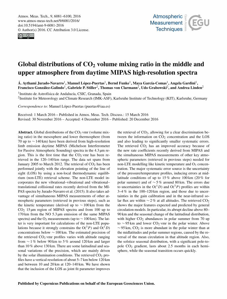
Figure 1. Regularization strength used in the retrieval of theCO2 vmr.

1 Introduction

Carbon dioxide, CO2, plays a major role in the radiative en-ergy budget of the atmosphere. Its 15 µm band is the majorinfrared cooling below around 120 km, and it also causes asignificant heating of the upper mesosphere by the absorptionof solar radiation in its near-infrared bands (see e.g. López-Puertas and Taylor, 2001). Hence, CO2 has a critical effecton the atmospheric temperature structure and therefore it isvery important to know its global (altitude and latitude) dis-tribution accurately (see e.g. Garcia et al., 2014).

CO2 was first measured in the upper atmosphere byin situ measurements carried out by rocket-borne massspectrometers (Offermann and Grossmann, 1973; Trinkset al., 1978; Trinks and Fricke, 1978). The Spectral In-frared Rocket Experiment (SPIRE) measured its 15 µm non-LTE (non-local thermodynamic equilibrium) emission (Stairet al., 1985). The Improved Stratospheric and MesosphericSounder (ISAMS) aboard the Upper Atmosphere ResearchSatellite (UARS) carried out 4.6 µm global measurementsperforming simultaneous measurements of temperature andpressure up to 80 km (López-Puertas et al., 1998; Zaragozaet al., 2000). CO2 number densities were retrieved fromdaytime limb radiance measured by the Cryogenic InfraredSpectrometers and Telescopes for the Atmosphere (CRISTA)measurements in the 60–130 km region (Kaufmann et al.,2002). For a complete review of early measurements until2000 see López-Puertas et al. (2000). More recently, twosatellite CO2 data sets have been made available. The Fouriertransform spectrometer on the Canadian Atmospheric Chem-istry Experiment (ACE-FTS) has measured the CO2 vmr inthe mesosphere and lower thermosphere (70 to 120 km) byusing the solar occultation technique. This approach has theadvantage of being free from non-LTE effects (and the er-rors associated to the knowledge of the non-LTE population

of the emitting states) but provides limited latitudinal cover-age (Beagley et al., 2010). Almost simultaneously with ACE,the Sounding of the Atmosphere using Broadband Emis-sion Radiometry (SABER), on board the NASA Thermo-sphere Ionosphere Energetics and Dynamics (TIMED), hasbeen measuring the atmospheric limb radiance in the 15 and4.3 µm channels. Rezac et al. (2015) applied a simultaneoustemperature–CO2 vmr retrieval to these measurements andproduced a long (13-year) database of CO2 in the middle andupper atmosphere.

In this paper we describe the inversion of CO2 vmr fromMIPAS (Michelson Interferometer for Passive AtmosphericSounding) high-resolution daytime limb emission spectra inthe 4.3 µm region. MIPAS is able to discriminate the contri-butions of the many CO2 bands that give rise to the 4.3 µmatmospheric emission; thus in a previous work it allowed usto obtain a more accurate knowledge of the CO2 non-LTEprocesses that control the population of the emitting levelsnear 4.3 µm (Jurado-Navarro et al., 2015). In that work thelarge impact of the new collisional rates on the limb atmo-spheric radiance near 4.3 µm was demonstrated (see Figs. 11and 12 in that paper). Several tests performed in that studyhave also shown a substantial effect on the retrieved CO2.Therefore, the use of those retrieved collisional rates allowedus to retrieve CO2 with a much better accuracy in the presentwork than in previous limb emission measurements. In addi-tion, the high spectral resolution allows for a proper selectionof the spectral points (optically thin and moderate points ofthe lines of the bands) containing the largest amount of in-formation at different tangent heights, which constrains theretrieval better than an integral wideband radiance measure-ment.

In Sect. 2 we describe the MIPAS instrument and the mea-surements, and in Sect. 3 the retrieval method and the set-up.The advantages of using the CO2-LOS (line of sight) jointretrieval are discussed in Sect. 4. In Sect. 5 we discuss themajor characteristics of the retrieved CO2 vmr and the erroranalysis. Finally, in Sect. 6 we provide and discuss a monthlyclimatology based on the data retrieved in 2010 and 2011. Avalidation and comparison of MIPAS CO2 data with ACEand SABER measurements, as well as with Whole Atmo-sphere Community Climate Model (WACCM) simulations,are to be presented in a future paper.

2 MIPAS observations

The MIPAS instrument is a mid-infrared limb emission spec-trometer designed and operated for measurements of atmo-spheric trace species from space (Fischer et al., 2008). It waspart of the payload of Envisat launched on 1 March 2002 witha sun-synchronous polar orbit of 98.55◦ N inclination and analtitude of 800 km. MIPAS had a global coverage from poleto pole passing the equator from north to south at 10:00 lo-cal time, 14.3 times a day and taking daytime and night-time

Atmos. Meas. Tech., 9, 6081–6100, 2016 www.atmos-meas-tech.net/9/6081/2016/

Á. A. Jurado-Navarro et al.: CO2 measurements from MIPAS 6083

profiles of spectra. The instrument’s field-of-view is 30 km inthe horizontal and approximately 3 km in the vertical direc-tion. From January 2005 until the end of Envisat’s operationson 8 April 2012, MIPAS measured at a optimized spectralresolution of 0.0625 cm−1.

The MIPAS instrument sounded the middle and upper at-mospheres in three measurements modes: MA (middle at-mosphere), UA (upper atmosphere) and NLC (noctilucentclouds). The UA mode, scanning the limb from 42 to 172 km,was specifically devised for measuring the thermospherictemperature and CO2 and NO abundances. In the MA andNLC modes, MIPAS took spectra up to 102 km only. How-ever, since many lines of the CO2 fundamental band (thosewith a larger signal) are still optically thick at this tangentheight and above, they reduce the sensitivity to the retrievedCO2 below 102 km. Thus, having measurements above thataltitude are very important for retrieving the CO2 in the opti-cally thin regime and hence better constraining the CO2 vmrbelow. As a consequence, the retrieval set-up and the de-rived CO2 presented here, data version v5r_CO2_622, cor-respond to the UA observation mode. Only daytime datawere used since the night-time observations are very noisyand non-LTE processes are not known that accurately. Notethat the three MIPAS modes have very similar temporal andlatitudinal coverages. Hence the retrieval of CO2 from theMA and NLC modes would not significantly extend thecoverage of the CO2 UA database. The limb vertical sam-pling of the UA mode is 5 km from 172 km down to 102 kmand 3 km below, recording a rear viewing sequence of 35spectra every 63 s. Its along-track horizontal sampling is ofabout 515 km (De Laurentis, 2005; Oelhaf, 2008). VersionV5 (5.02/5.06) of the L1b calibrated and geo-located spec-tra processed by the European Space Agency (ESA; Perronet al., 2010; Raspollini et al., 2010) were used here for theretrieval of CO2 and for all other parameters used in its re-trieval, namely, pressure/temperature and ozone.

3 The retrieval method and its set-up

Carbon dioxide vmr profiles together with the elevationpointing of the line of sight (LOS) are retrieved using the MI-PAS level 2 processor developed and operated by the Instituteof Meteorology and Climate Research (IMK) together withthe Instituto de Astrofísica de Andalucía (IAA). The proces-sor is based on a constrained non-linear least squares algo-rithm with Levenberg–Marquardt damping (von Clarmannet al., 2003). Its extension to retrievals with considerationof non-LTE (i.e. CO, NO and NO2) is described by Funkeet al. (2001). Non-LTE vibrational populations of CO2 aremodelled with the Generic RAdiative traNsfer AnD non-LTEpopulation Algorithm (GRANADA; Funke et al., 2012; seemore details below) within each iteration of the retrieval.

Following the scheme described by von Clarmann et al.(2003), the following retrieval equation is used:

xi+1 = xi +[KT S−1

y K+R+ λI]−1

×

{KTS−1

y [ymeas− y(xi)] −R(xi − xa)}, (1)

where K is the mmax× nmax Jacobian, containing the par-tial derivatives of allmmax simulated measurements y(x) un-der consideration with respect to all unknown parameters x,superscript T denotes a transposed matrix, x is the nmax–dimensional vector of unknown parameters and xa is therelated a priori information. The term ymeas is the mmax-dimensional vector of measurements under consideration,y(xi) is the forward modelled spectrum using parameters xifrom the i-th step of iteration. R is an nmax×nmax regulariza-tion matrix, and Sy is the mmax× mmax covariance matrix ofthe measurement. The term λI (tuning scalar times the unitymatrix) dampens the step width xi+1− xi , bends its direc-tion toward the direction of the steepest descent of the costfunction in the parameter space and prevents a single itera-tion from causing a jump of parameters x beyond the lineardomain around the current guess xi (Levenberg, 1944; Mar-quardt, 1963).

In our case, the column vector x contains the CO2 pro-file (103 elements), the LOS profile (23 elements) and theradiance offset (17 elements, one per each microwindow).The a priori profile, xa , for CO2 is taken from monthly zonalmeans of the Whole Atmosphere Community Climate Modelwith specified dynamics (SD-WACCM) simulations span-ning over the time period of the measurements (Garcia et al.,2014). SD-WACCM is constrained with output from NASA’sModern-Era Retrospective Analysis (MERRA) (Rieneckeret al., 2011) below approximately 1 hPa. Garcia et al. (2014)showed SD-WACCM simulations for Prandtl numbers (Pr )of 4 (standard) and 2, corresponding to lower and higher eddydiffusion coefficients respectively. Here we used the simu-lations for Pr = 2, which gives an overall better agreementwith ACE CO and CO2 and MIPAS CO (Garcia et al., 2014).In this way we expect to have a faster convergence with noimpact of the a priori profile since the CO2 profile is regular-ized by means of a Tikhonov-type first-order smoothing con-straint (Tikhonov, 1963; see below). The a priori profile forthe elevation pointing of the line of sight (LOS) was takenfrom that retrieved from the 15 µm region (García-Comaset al., 2014).

Since in the target altitude range we use a smoothingconstraint only, x is not pushed towards the a priori pro-file but the latter constrains the shape of the resulting pro-file only. Sy is the covariance matrix characterizing themeasurement noise. Due to apodization (Norton and Beer,1976) this matrix contains off-diagonal elements. R is theconstraint matrix. CO2 is constrained by a Tikhonov-type(Tikhonov, 1963) squared first-order finite differences matrix(weighted by the grid-width) with altitude-dependent regu-

www.atmos-meas-tech.net/9/6081/2016/ Atmos. Meas. Tech., 9, 6081–6100, 2016


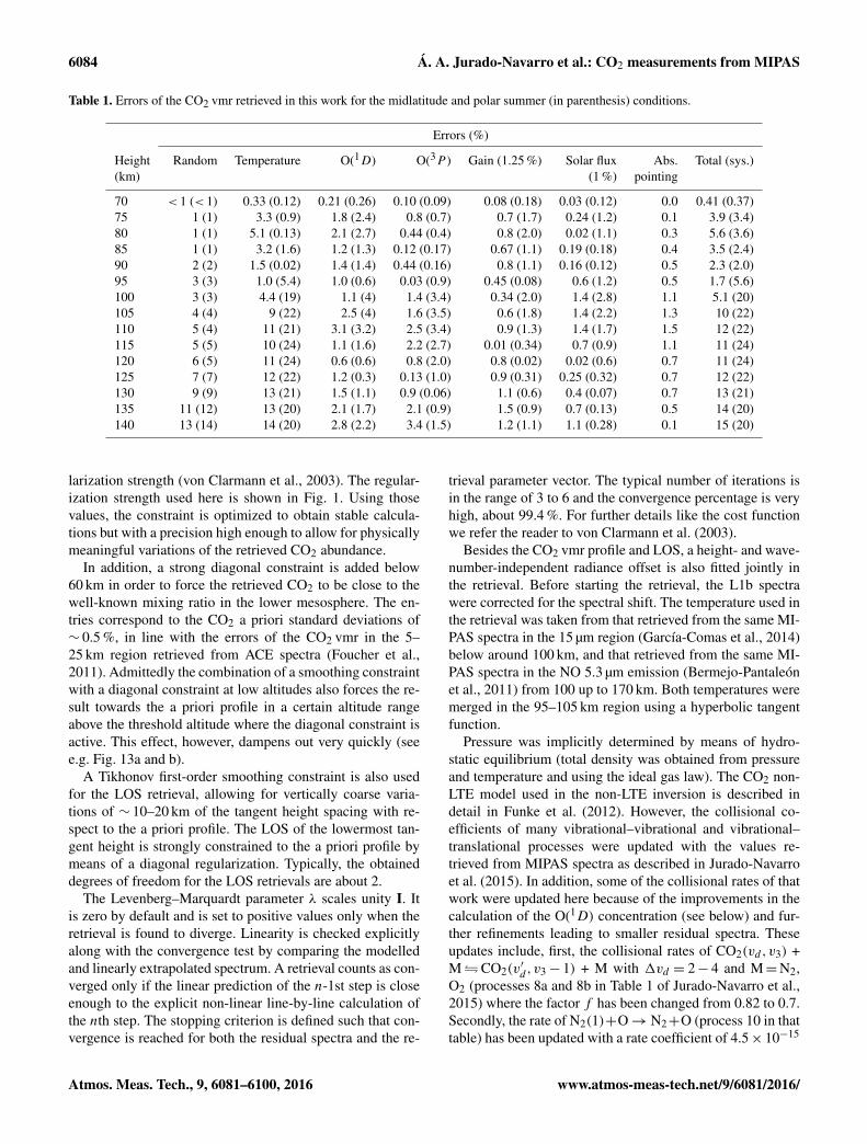
Table 1. Errors of the CO2 vmr retrieved in this work for the midlatitude and polar summer (in parenthesis) conditions.

Errors (%)

Height Random Temperature O(1D) O(3P ) Gain (1.25 %) Solar flux Abs. Total (sys.)(km) (1 %) pointing

70 < 1 (< 1) 0.33 (0.12) 0.21 (0.26) 0.10 (0.09) 0.08 (0.18) 0.03 (0.12) 0.0 0.41 (0.37)75 1 (1) 3.3 (0.9) 1.8 (2.4) 0.8 (0.7) 0.7 (1.7) 0.24 (1.2) 0.1 3.9 (3.4)80 1 (1) 5.1 (0.13) 2.1 (2.7) 0.44 (0.4) 0.8 (2.0) 0.02 (1.1) 0.3 5.6 (3.6)85 1 (1) 3.2 (1.6) 1.2 (1.3) 0.12 (0.17) 0.67 (1.1) 0.19 (0.18) 0.4 3.5 (2.4)90 2 (2) 1.5 (0.02) 1.4 (1.4) 0.44 (0.16) 0.8 (1.1) 0.16 (0.12) 0.5 2.3 (2.0)95 3 (3) 1.0 (5.4) 1.0 (0.6) 0.03 (0.9) 0.45 (0.08) 0.6 (1.2) 0.5 1.7 (5.6)100 3 (3) 4.4 (19) 1.1 (4) 1.4 (3.4) 0.34 (2.0) 1.4 (2.8) 1.1 5.1 (20)105 4 (4) 9 (22) 2.5 (4) 1.6 (3.5) 0.6 (1.8) 1.4 (2.2) 1.3 10 (22)110 5 (4) 11 (21) 3.1 (3.2) 2.5 (3.4) 0.9 (1.3) 1.4 (1.7) 1.5 12 (22)115 5 (5) 10 (24) 1.1 (1.6) 2.2 (2.7) 0.01 (0.34) 0.7 (0.9) 1.1 11 (24)120 6 (5) 11 (24) 0.6 (0.6) 0.8 (2.0) 0.8 (0.02) 0.02 (0.6) 0.7 11 (24)125 7 (7) 12 (22) 1.2 (0.3) 0.13 (1.0) 0.9 (0.31) 0.25 (0.32) 0.7 12 (22)130 9 (9) 13 (21) 1.5 (1.1) 0.9 (0.06) 1.1 (0.6) 0.4 (0.07) 0.7 13 (21)135 11 (12) 13 (20) 2.1 (1.7) 2.1 (0.9) 1.5 (0.9) 0.7 (0.13) 0.5 14 (20)140 13 (14) 14 (20) 2.8 (2.2) 3.4 (1.5) 1.2 (1.1) 1.1 (0.28) 0.1 15 (20)

larization strength (von Clarmann et al., 2003). The regular-ization strength used here is shown in Fig. 1. Using thosevalues, the constraint is optimized to obtain stable calcula-tions but with a precision high enough to allow for physicallymeaningful variations of the retrieved CO2 abundance.

In addition, a strong diagonal constraint is added below60 km in order to force the retrieved CO2 to be close to thewell-known mixing ratio in the lower mesosphere. The en-tries correspond to the CO2 a priori standard deviations of∼ 0.5 %, in line with the errors of the CO2 vmr in the 5–25 km region retrieved from ACE spectra (Foucher et al.,2011). Admittedly the combination of a smoothing constraintwith a diagonal constraint at low altitudes also forces the re-sult towards the a priori profile in a certain altitude rangeabove the threshold altitude where the diagonal constraint isactive. This effect, however, dampens out very quickly (seee.g. Fig. 13a and b).

A Tikhonov first-order smoothing constraint is also usedfor the LOS retrieval, allowing for vertically coarse varia-tions of ∼ 10–20 km of the tangent height spacing with re-spect to the a priori profile. The LOS of the lowermost tan-gent height is strongly constrained to the a priori profile bymeans of a diagonal regularization. Typically, the obtaineddegrees of freedom for the LOS retrievals are about 2.

The Levenberg–Marquardt parameter λ scales unity I. Itis zero by default and is set to positive values only when theretrieval is found to diverge. Linearity is checked explicitlyalong with the convergence test by comparing the modelledand linearly extrapolated spectrum. A retrieval counts as con-verged only if the linear prediction of the n-1st step is closeenough to the explicit non-linear line-by-line calculation ofthe nth step. The stopping criterion is defined such that con-vergence is reached for both the residual spectra and the re-

trieval parameter vector. The typical number of iterations isin the range of 3 to 6 and the convergence percentage is veryhigh, about 99.4 %. For further details like the cost functionwe refer the reader to von Clarmann et al. (2003).

Besides the CO2 vmr profile and LOS, a height- and wave-number-independent radiance offset is also fitted jointly inthe retrieval. Before starting the retrieval, the L1b spectrawere corrected for the spectral shift. The temperature used inthe retrieval was taken from that retrieved from the same MI-PAS spectra in the 15 µm region (García-Comas et al., 2014)below around 100 km, and that retrieved from the same MI-PAS spectra in the NO 5.3 µm emission (Bermejo-Pantaleónet al., 2011) from 100 up to 170 km. Both temperatures weremerged in the 95–105 km region using a hyperbolic tangentfunction.

Pressure was implicitly determined by means of hydro-static equilibrium (total density was obtained from pressureand temperature and using the ideal gas law). The CO2 non-LTE model used in the non-LTE inversion is described indetail in Funke et al. (2012). However, the collisional co-efficients of many vibrational–vibrational and vibrational–translational processes were updated with the values re-trieved from MIPAS spectra as described in Jurado-Navarroet al. (2015). In addition, some of the collisional rates of thatwork were updated here because of the improvements in thecalculation of the O(1D) concentration (see below) and fur-ther refinements leading to smaller residual spectra. Theseupdates include, first, the collisional rates of CO2(vd ,v3) +M�CO2(v

′

d ,v3− 1) + M with 1vd = 2− 4 and M=N2,O2 (processes 8a and 8b in Table 1 of Jurado-Navarro et al.,2015) where the factor f has been changed from 0.82 to 0.7.Secondly, the rate of N2(1)+O→ N2+O (process 10 in thattable) has been updated with a rate coefficient of 4.5× 10−15



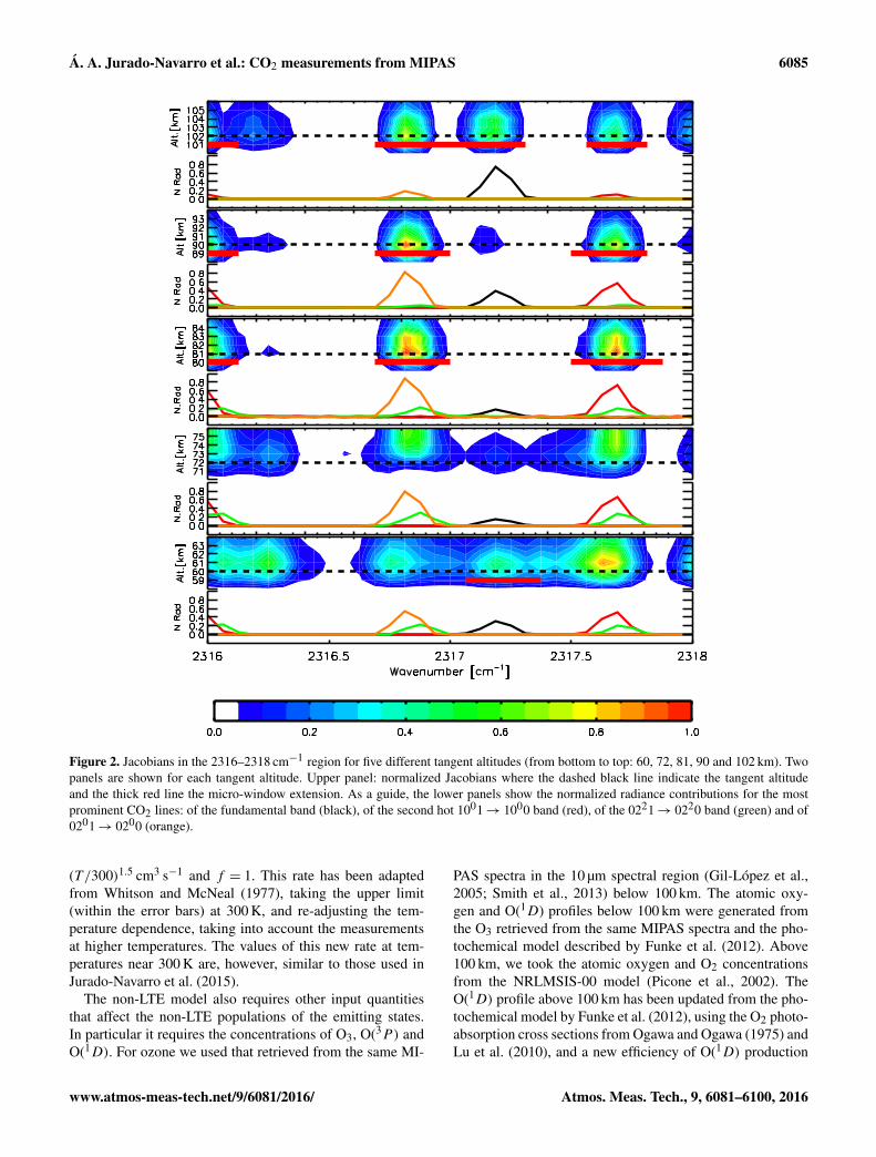
Figure 2. Jacobians in the 2316–2318 cm−1 region for five different tangent altitudes (from bottom to top: 60, 72, 81, 90 and 102 km). Twopanels are shown for each tangent altitude. Upper panel: normalized Jacobians where the dashed black line indicate the tangent altitudeand the thick red line the micro-window extension. As a guide, the lower panels show the normalized radiance contributions for the mostprominent CO2 lines: of the fundamental band (black), of the second hot 1001→ 1000 band (red), of the 0221→ 0220 band (green) and of0201→ 0200 (orange).

(T/300)1.5 cm3 s−1 and f = 1. This rate has been adaptedfrom Whitson and McNeal (1977), taking the upper limit(within the error bars) at 300 K, and re-adjusting the tem-perature dependence, taking into account the measurementsat higher temperatures. The values of this new rate at tem-peratures near 300 K are, however, similar to those used inJurado-Navarro et al. (2015).

The non-LTE model also requires other input quantitiesthat affect the non-LTE populations of the emitting states.In particular it requires the concentrations of O3, O(3P) andO(1D). For ozone we used that retrieved from the same MI-

PAS spectra in the 10 µm spectral region (Gil-López et al.,2005; Smith et al., 2013) below 100 km. The atomic oxy-gen and O(1D) profiles below 100 km were generated fromthe O3 retrieved from the same MIPAS spectra and the pho-tochemical model described by Funke et al. (2012). Above100 km, we took the atomic oxygen and O2 concentrationsfrom the NRLMSIS-00 model (Picone et al., 2002). TheO(1D) profile above 100 km has been updated from the pho-tochemical model by Funke et al. (2012), using the O2 photo-absorption cross sections from Ogawa and Ogawa (1975) andLu et al. (2010), and a new efficiency of O(1D) production



2300 2320 2340 2360 2380Wavenumber [cm-1]

60

80

100

120

140

Tan

gent

hei

ght [

km]

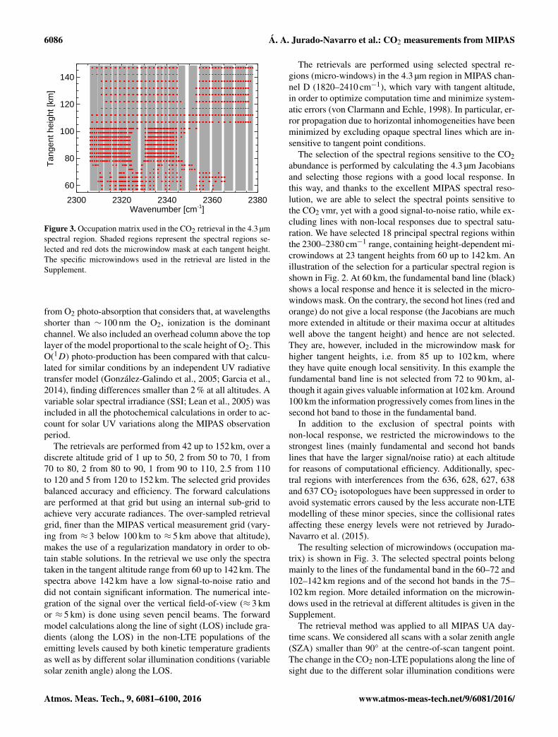
Figure 3. Occupation matrix used in the CO2 retrieval in the 4.3 µmspectral region. Shaded regions represent the spectral regions se-lected and red dots the microwindow mask at each tangent height.The specific microwindows used in the retrieval are listed in theSupplement.

from O2 photo-absorption that considers that, at wavelengthsshorter than ∼ 100 nm the O2, ionization is the dominantchannel. We also included an overhead column above the toplayer of the model proportional to the scale height of O2. ThisO(1D) photo-production has been compared with that calcu-lated for similar conditions by an independent UV radiativetransfer model (González-Galindo et al., 2005; Garcia et al.,2014), finding differences smaller than 2 % at all altitudes. Avariable solar spectral irradiance (SSI; Lean et al., 2005) wasincluded in all the photochemical calculations in order to ac-count for solar UV variations along the MIPAS observationperiod.

The retrievals are performed from 42 up to 152 km, over adiscrete altitude grid of 1 up to 50, 2 from 50 to 70, 1 from70 to 80, 2 from 80 to 90, 1 from 90 to 110, 2.5 from 110to 120 and 5 from 120 to 152 km. The selected grid providesbalanced accuracy and efficiency. The forward calculationsare performed at that grid but using an internal sub-grid toachieve very accurate radiances. The over-sampled retrievalgrid, finer than the MIPAS vertical measurement grid (vary-ing from ≈ 3 below 100 km to ≈ 5 km above that altitude),makes the use of a regularization mandatory in order to ob-tain stable solutions. In the retrieval we use only the spectrataken in the tangent altitude range from 60 up to 142 km. Thespectra above 142 km have a low signal-to-noise ratio anddid not contain significant information. The numerical inte-gration of the signal over the vertical field-of-view (≈ 3 kmor ≈ 5 km) is done using seven pencil beams. The forwardmodel calculations along the line of sight (LOS) include gra-dients (along the LOS) in the non-LTE populations of theemitting levels caused by both kinetic temperature gradientsas well as by different solar illumination conditions (variablesolar zenith angle) along the LOS.

The retrievals are performed using selected spectral re-gions (micro-windows) in the 4.3 µm region in MIPAS chan-nel D (1820–2410 cm−1), which vary with tangent altitude,in order to optimize computation time and minimize system-atic errors (von Clarmann and Echle, 1998). In particular, er-ror propagation due to horizontal inhomogeneities have beenminimized by excluding opaque spectral lines which are in-sensitive to tangent point conditions.

The selection of the spectral regions sensitive to the CO2abundance is performed by calculating the 4.3 µm Jacobiansand selecting those regions with a good local response. Inthis way, and thanks to the excellent MIPAS spectral reso-lution, we are able to select the spectral points sensitive tothe CO2 vmr, yet with a good signal-to-noise ratio, while ex-cluding lines with non-local responses due to spectral satu-ration. We have selected 18 principal spectral regions withinthe 2300–2380 cm−1 range, containing height-dependent mi-crowindows at 23 tangent heights from 60 up to 142 km. Anillustration of the selection for a particular spectral region isshown in Fig. 2. At 60 km, the fundamental band line (black)shows a local response and hence it is selected in the micro-windows mask. On the contrary, the second hot lines (red andorange) do not give a local response (the Jacobians are muchmore extended in altitude or their maxima occur at altitudeswell above the tangent height) and hence are not selected.They are, however, included in the microwindow mask forhigher tangent heights, i.e. from 85 up to 102 km, wherethey have quite enough local sensitivity. In this example thefundamental band line is not selected from 72 to 90 km, al-though it again gives valuable information at 102 km. Around100 km the information progressively comes from lines in thesecond hot band to those in the fundamental band.

In addition to the exclusion of spectral points withnon-local response, we restricted the microwindows to thestrongest lines (mainly fundamental and second hot bandslines that have the larger signal/noise ratio) at each altitudefor reasons of computational efficiency. Additionally, spec-tral regions with interferences from the 636, 628, 627, 638and 637 CO2 isotopologues have been suppressed in order toavoid systematic errors caused by the less accurate non-LTEmodelling of these minor species, since the collisional ratesaffecting these energy levels were not retrieved by Jurado-Navarro et al. (2015).

The resulting selection of microwindows (occupation ma-trix) is shown in Fig. 3. The selected spectral points belongmainly to the lines of the fundamental band in the 60–72 and102–142 km regions and of the second hot bands in the 75–102 km region. More detailed information on the microwin-dows used in the retrieval at different altitudes is given in theSupplement.

The retrieval method was applied to all MIPAS UA day-time scans. We considered all scans with a solar zenith angle(SZA) smaller than 90◦ at the centre-of-scan tangent point.The change in the CO2 non-LTE populations along the line ofsight due to the different solar illumination conditions were



0 100 200 300 400Mixing ratio [ppmv]

60

80

100

120

140

Alti

tude

[km

]

A prioriRetrievedTrue

-40 -30 -20 -10 0 10Relative difference [%]


60

80

100

120

140

Alti

tude

[km

]


0 20 40 60Relative difference [%]


60

80

100

120

140

Alti

tude

[km

]


-30 -20 -10 0 10 20Relative difference [%]


60

80

100

120

140

Alti

tude

[km

]A prioriRetrievedTrue

-20 0 20Relative difference [%]

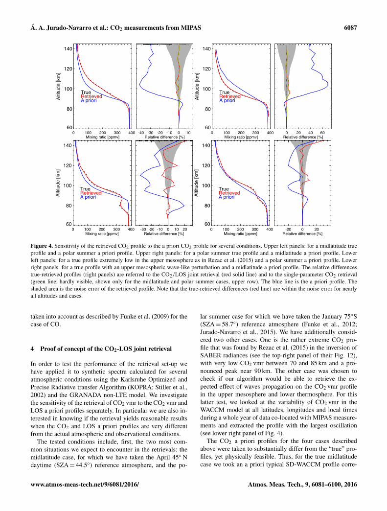
Figure 4. Sensitivity of the retrieved CO2 profile to the a priori CO2 profile for several conditions. Upper left panels: for a midlatitude trueprofile and a polar summer a priori profile. Upper right panels: for a polar summer true profile and a midlatitude a priori profile. Lowerleft panels: for a true profile extremely low in the upper mesosphere as in Rezac et al. (2015) and a polar summer a priori profile. Lowerright panels: for a true profile with an upper mesospheric wave-like perturbation and a midlatitude a priori profile. The relative differencestrue-retrieved profiles (right panels) are referred to the CO2/LOS joint retrieval (red solid line) and to the single-parameter CO2 retrieval(green line, hardly visible, shown only for the midlatitude and polar summer cases, upper row). The blue line is the a priori profile. Theshaded area is the noise error of the retrieved profile. Note that the true-retrieved differences (red line) are within the noise error for nearlyall altitudes and cases.

taken into account as described by Funke et al. (2009) for thecase of CO.

4 Proof of concept of the CO2-LOS joint retrieval

In order to test the performance of the retrieval set-up wehave applied it to synthetic spectra calculated for severalatmospheric conditions using the Karlsruhe Optimized andPrecise Radiative transfer Algorithm (KOPRA; Stiller et al.,2002) and the GRANADA non-LTE model. We investigatethe sensitivity of the retrieval of CO2 vmr to the CO2 vmr andLOS a priori profiles separately. In particular we are also in-terested in knowing if the retrieval yields reasonable resultswhen the CO2 and LOS a priori profiles are very differentfrom the actual atmospheric and observational conditions.

The tested conditions include, first, the two most com-mon situations we expect to encounter in the retrievals: themidlatitude case, for which we have taken the April 45◦ Ndaytime (SZA= 44.5◦) reference atmosphere, and the po-

lar summer case for which we have taken the January 75◦S(SZA= 58.7◦) reference atmosphere (Funke et al., 2012;Jurado-Navarro et al., 2015). We have additionally consid-ered two other cases. One is the rather extreme CO2 pro-file that was found by Rezac et al. (2015) in the inversion ofSABER radiances (see the top-right panel of their Fig. 12),with very low CO2 vmr between 70 and 85 km and a pro-nounced peak near 90 km. The other case was chosen tocheck if our algorithm would be able to retrieve the ex-pected effect of waves propagation on the CO2 vmr profilein the upper mesosphere and lower thermosphere. For thislatter test, we looked at the variability of CO2 vmr in theWACCM model at all latitudes, longitudes and local timesduring a whole year of data co-located with MIPAS measure-ments and extracted the profile with the largest oscillation(see lower right panel of Fig. 4).

The CO2 a priori profiles for the four cases describedabove were taken to substantially differ from the “true” pro-files, yet physically feasible. Thus, for the true midlatitudecase we took an a priori typical SD-WACCM profile corre-



-0.03 -0.02 -0.01 0.00 0.01 0.02 0.03LOS difference [km]

60

80

100

120

140A

ltitu

de [k

m]

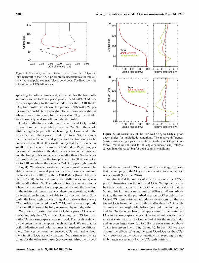
Figure 5. Sensitivity of the retrieved LOS (from the CO2–LOSjoint retrieval) to the CO2 a priori profile uncertainties for midlati-tude (red) and polar summer (black) conditions. The lines show theretrieved–true LOS differences.

sponding to polar summer and, viceversa, for the true polarsummer case we took as a priori profile the SD-WACCM pro-file corresponding to the midlatitudes. For the SABER-likeCO2 true profile we choose the previous SD-WACCM po-lar summer profile (corresponding to the seasonal conditionswhere it was found) and, for the wave-like CO2 true profile,we choose a typical smooth midlatitude profile.

Under midlatitude conditions, the retrieved CO2 profilediffers from the true profile by less than 2–3 % in the wholealtitude region (upper left panels in Fig. 4). Compared to thedifference with the a priori profile (up to 40 %), the agree-ment between the retrieved profile and the true one can beconsidered excellent. It is worth noting that the difference issmaller than the noise error at all altitudes. Regarding po-lar summer conditions, the differences between the retrievedand the true profiles are generally smaller than 2 % (the a pri-ori profile differs from the true profile up to 60 %) except at95 to 110 km where the range is 2–4 % (upper right panelsin Fig. 4). We also demonstrate that our algorithm would beable to retrieve unusual profiles such as those encounteredby Rezac et al. (2015) in the SABER data (lower left pan-els in Fig. 4). Retrieved minus true differences are gener-ally smaller than 3 %. The only exceptions occur at altitudeswhere the true profile has abrupt gradients (note the blue linein the relative difference panel) where our algorithm, withinits vertical resolution, is not able to fully recover them. Sim-ilarly, the lower right panels of Fig. 4 also shows that a wavyCO2 profile as predicted by WACCM, with a wave amplitudeof about 20 %, would be fully recovered by our algorithm.

We have also tested the effect of the a priori CO2 whenretrieving only the CO2 vmr and keeping the LOS fixed, i.e.with CO2 as a single-parameter retrieval. The result is shownby the green line in the upper panels of Fig. 4. We see that forboth midlatitude and polar summer atmospheric conditions,the differences between the retrieved CO2 with and withoutthe joint fit of LOS are only marginal. Very similar results arefound for the other two cases (not shown). Also, the inspec-


60

80

100

120

140

Alti

tude

[km

]

Single retrievedJoint retrievedTrue

-6 -4 -2 0 2 4 6Relative difference [%]


60

80

100

120

140

Alti

tude

[km

]

Single retrievedJoint retrievedTrue

-6 -4 -2 0 2 4 6Relative difference [%]

(a)

(b)

Figure 6. (a) Sensitivity of the retrieved CO2 to LOS a prioriuncertainties for midlatitude conditions. The relative differences(retrieved–true) (right panel) are referred to the joint CO2-LOS re-trieval (red solid line) and to the single-parameter CO2 retrieval(green line). (b) As (a) but for polar summer conditions.

tion of the retrieved LOS in the joint fit case (Fig. 5) showsthat the mapping of the CO2 a priori uncertainties on the LOSis very small (less than 20 m).

We also tested the impact of a perturbation of the LOS apriori information on the retrieved CO2. We applied a sinefunction perturbation to the LOS with a value of 0 m at60 and 142 km and a maximum of 200 m at 90 km. Above90 km, the use of the perturbed a priori LOS profile in theCO2–LOS joint retrieval introduces deviations of the re-trieved CO2 from the true profile smaller than 1–2 %, whiledifferences are negligible below (see red line in Fig. 6aand b). On the other hand, the application of the perturbedLOS in the single-parameter CO2 retrieval introduces a sig-nificant systematic error of up to 3–4 % for the midlatitudesand an even larger error (up to 5 %) for polar summer above70 km (see green line in Fig. 6a and b). In Sect. 5.2 we alsodiscuss the effects of using the joint CO2-LOS or the CO2-only retrievals on the total systematic error, resulting in a no-tably larger uncertainty for the CO2-only retrieval.



-0.1 0.0 0.1 0.2 0.3 0.4 0.5Averaging Kernel

60

80

100

120

140

Alti

tude

[km

]

-0.1 0.0 0.1 0.2 0.3 0.4 0.5Averaging Kernel

60

80

100

120

140

Alti

tude

[km

](a)

(b)

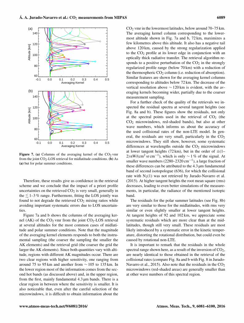
Figure 7. (a) Columns of the averaging kernel of the CO2 vmrfrom the joint CO2-LOS retrieval for midlatitude conditions. (b) As(a) but for polar summer conditions.

Therefore, these results give us confidence in the retrievalscheme and we conclude that the impact of a priori profileuncertainties on the retrieved CO2 is very small, generally inthe . 1–3 % range. Furthermore, fitting the LOS jointly wasfound to not degrade the retrieved CO2 mixing ratios whileavoiding important systematic errors due to LOS uncertain-ties.

Figure 7a and b shows the columns of the averaging ker-nel (AK) of the CO2 vmr from the joint CO2-LOS retrievalat several altitudes for the most common cases of midlati-tude and polar summer conditions. Note that the magnitudeof the averaging kernel elements responds to both the instru-mental sampling (the coarser the sampling the smaller theAK elements) and the retrieval grid (the coarser the grid thelarger the AK elements). Since both quantities vary with alti-tude, regions with different AK magnitudes occur. There aretwo clear regions with higher sensitivity, one ranging fromaround 75 to 95 km and another from ∼ 105 to 135 km. Inthe lower region most of the information comes from the sec-ond hot bands (as discussed above) and, in the upper region,from the first, mainly fundamental 4.3 µm bands. There is aclear region in between where the sensitivity is smaller. It isalso noticeable that, even after the careful selection of themicrowindows, it is difficult to obtain information about the

CO2 vmr in the lowermost latitudes, below around 70–75 km.The averaging kernel column corresponding to the lower-most altitude shown in Fig. 7a and b, 72 km, maximizes afew kilometres above this altitude. It also has a negative tailabove 120 km, caused by the strong regularization appliedto the CO2 profile at its lower edge in conjunction with anoptically thick radiative transfer. The retrieval algorithm re-sponds to a positive perturbation of the CO2 in the stronglyregularized profile range (below 70 km) with a reduction ofthe thermospheric CO2 column (i.e. reduction of absorption).Similar features are shown for the averaging kernel columnscorresponding to altitudes below 72 km. The decrease of thevertical resolution above ∼ 120 km is evident, with the av-eraging kernels becoming wider, partially due to the coarsermeasurement sampling.

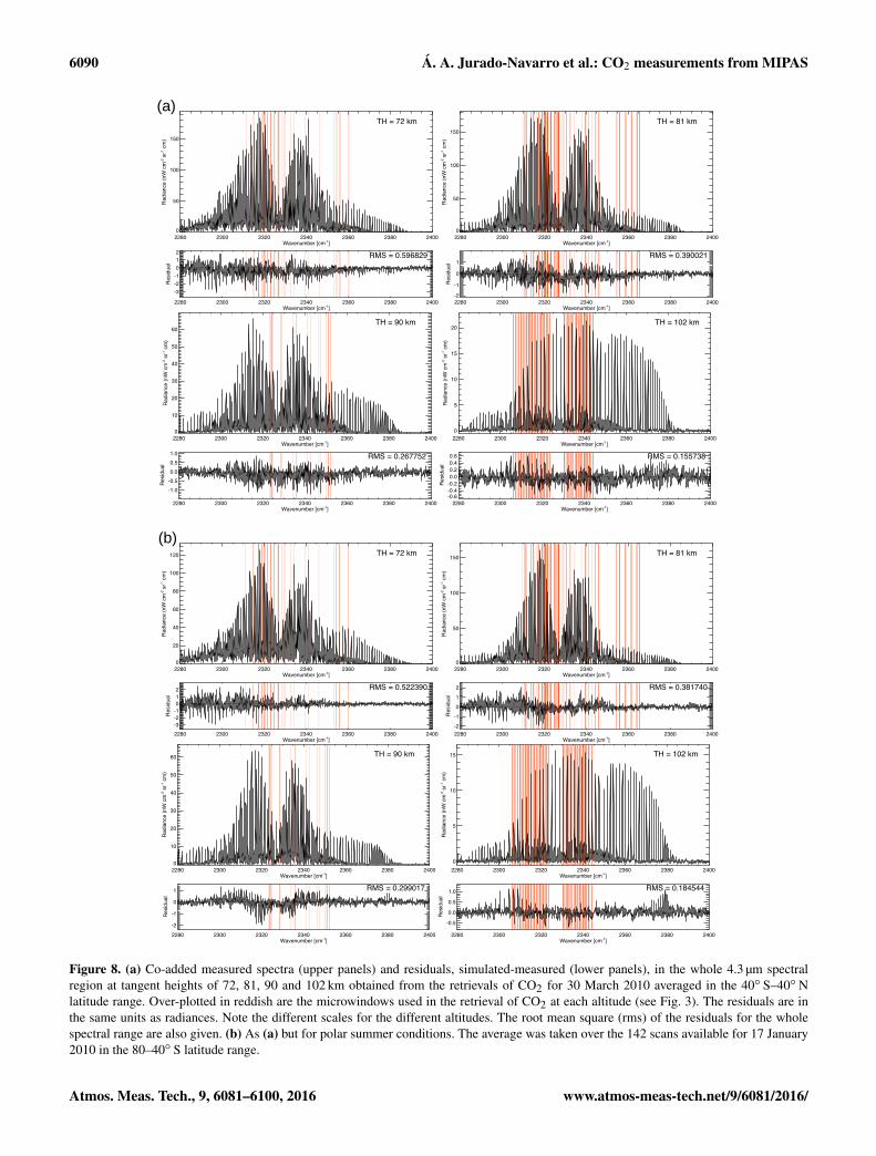
For a further check of the quality of the retrievals we in-spected the residual spectra at several tangent heights (seeFig. 8a and b). These figures show the residuals, not onlyat the spectral points used in the retrieval of CO2 (theCO2 microwindows, red-shaded bands), but also at otherwave numbers, which informs us about the accuracy ofthe used collisional rates of the non-LTE model. In gen-eral, the residuals are very small, particularly in the CO2microwindows. They still show, however, some systematicdifferences at wavelengths outside the CO2 microwindowsat lower tangent heights (72 km), but in the order of ±(1–2) nW/(cm2 sr cm−1), which is only ∼ 1 % of the signal. Atsmaller wave numbers (2280–2320 cm−1), a large fraction ofthese differences can be attributed to the 4.3 µm fundamentalband of second isotopologue (636), for which the collisionalrate with N2(1) was not retrieved by Jurado-Navarro et al.(2015). At higher tangent heights the root mean square (rms)decreases, leading to even better simulations of the measure-ments, in particular, the radiance of the mentioned isotopicband.

The residuals for the polar summer latitudes (see Fig. 8b)are very similar to those for the midlatitudes, with rms verysimilar or even slightly smaller at lower tangent heights.At tangent heights of 92 and 102 km, we appreciate somesystematic residuals which are more clear than at the mid-latitudes, though still very small. These residuals are mostlikely introduced by a systematic error in the kinetic temper-ature, distorting the rotational distribution, but could even becaused by rotational non-LTE.

It is important to remark that the residuals in the wholespectral range shown here, as a result of the inversion of CO2,are nearly identical to those obtained in the retrieval of thecollisional rates (compare Fig. 8a and b with Fig. 8 in Jurado-Navarro et al., 2015). Also note that the residuals in the CO2microwindows (red-shaded areas) are generally smaller thanat other wave numbers of this spectral region.



2280 2300 2320 2340 2360 2380 2400Wavenumber [cm-1]

0

50

100

150

Rad

ianc

e (n

W c

m-2 s

r-1 c

m)

TH = 72 km

2280 2300 2320 2340 2360 2380 2400Wavenumber [cm-1]

-3

-2

-1

0

12

Res

idua

l

RMS = 0.596829

2280 2300 2320 2340 2360 2380 2400Wavenumber [cm-1]

0

50

100

150

Rad

ianc

e (n

W c

m-2 s

r-1 c

m)

TH = 81 km

2280 2300 2320 2340 2360 2380 2400Wavenumber [cm-1]

-2

-1

0

1

Res

idua

l

RMS = 0.390021

2280 2300 2320 2340 2360 2380 2400Wavenumber [cm-1]

0

10

20

30

40

50

60

Rad

ianc

e (n

W c

m-2 s

r-1 c

m)

TH = 90 km

2280 2300 2320 2340 2360 2380 2400Wavenumber [cm-1]

-1.0

-0.5

0.0

0.5

1.0

Res

idua

l

RMS = 0.267752

2280 2300 2320 2340 2360 2380 2400Wavenumber [cm-1]

0

5

10

15

20

Rad

ianc

e (n

W c

m-2 s

r-1 c

m)

TH = 102 km

2280 2300 2320 2340 2360 2380 2400Wavenumber [cm-1]

-0.6-0.4-0.20.00.20.40.6

Res

idua

l

RMS = 0.155738

2280 2300 2320 2340 2360 2380 2400Wavenumber [cm-1]

0

20

40

60

80

100

120

Rad

ianc

e (n

W c

m-2 s

r-1 c

m)

TH = 72 km

2280 2300 2320 2340 2360 2380 2400Wavenumber [cm-1]

-3-2-1012

Res

idua

l

RMS = 0.522390

2280 2300 2320 2340 2360 2380 2400Wavenumber [cm-1]

0

50

100

150

Rad

ianc

e (n

W c

m-2 s

r-1 c

m)

TH = 81 km

2280 2300 2320 2340 2360 2380 2400Wavenumber [cm-1]

-2

-1

0

1

2

Res

idua

l

RMS = 0.381740

2280 2300 2320 2340 2360 2380 2400Wavenumber [cm-1]

0

10

20

30

40

50

60

Rad

ianc

e (n

W c

m-2 s

r-1 c

m)

TH = 90 km

2280 2300 2320 2340 2360 2380 2400Wavenumber [cm-1]

-2

-1

0

1

Res

idua

l

RMS = 0.299017

2280 2300 2320 2340 2360 2380 2400Wavenumber [cm-1]

0

5

10

15

Rad

ianc

e (n

W c

m-2 s

r-1 c

m)

TH = 102 km

2280 2300 2320 2340 2360 2380 2400Wavenumber [cm-1]

-0.5

0.0

0.5

1.0

Res

idua

l

RMS = 0.184544

(a)

(b)

Figure 8. (a) Co-added measured spectra (upper panels) and residuals, simulated-measured (lower panels), in the whole 4.3 µm spectralregion at tangent heights of 72, 81, 90 and 102 km obtained from the retrievals of CO2 for 30 March 2010 averaged in the 40◦ S–40◦ Nlatitude range. Over-plotted in reddish are the microwindows used in the retrieval of CO2 at each altitude (see Fig. 3). The residuals are inthe same units as radiances. Note the different scales for the different altitudes. The root mean square (rms) of the residuals for the wholespectral range are also given. (b) As (a) but for polar summer conditions. The average was taken over the 142 scans available for 17 January2010 in the 80–40◦ S latitude range.



1 Feb 1 Apr 1 Jun 1 Aug 1 Oct 1 Dec

-50

0

50La

titud

e [d

eg]

Chi2

30.0

40.0

40.0

5

0.0

50.0

6

0.0

60.0

7

0.0

70.0

70.0

8

0.0

80.0

80.0

90.0

1.25 1.30 1.35 1.40 1.45 1.50

1 Feb 1 Apr 1 Jun 1 Aug 1 Oct 1 Dec

-50

0

50

dof

30.0

40.0

40.0

5

0.0

50.0

6

0.0

60.0

7

0.0

70.0

70.0

8

0.0

80.0

80.0

90.0

2 3 4 5 6 7 8

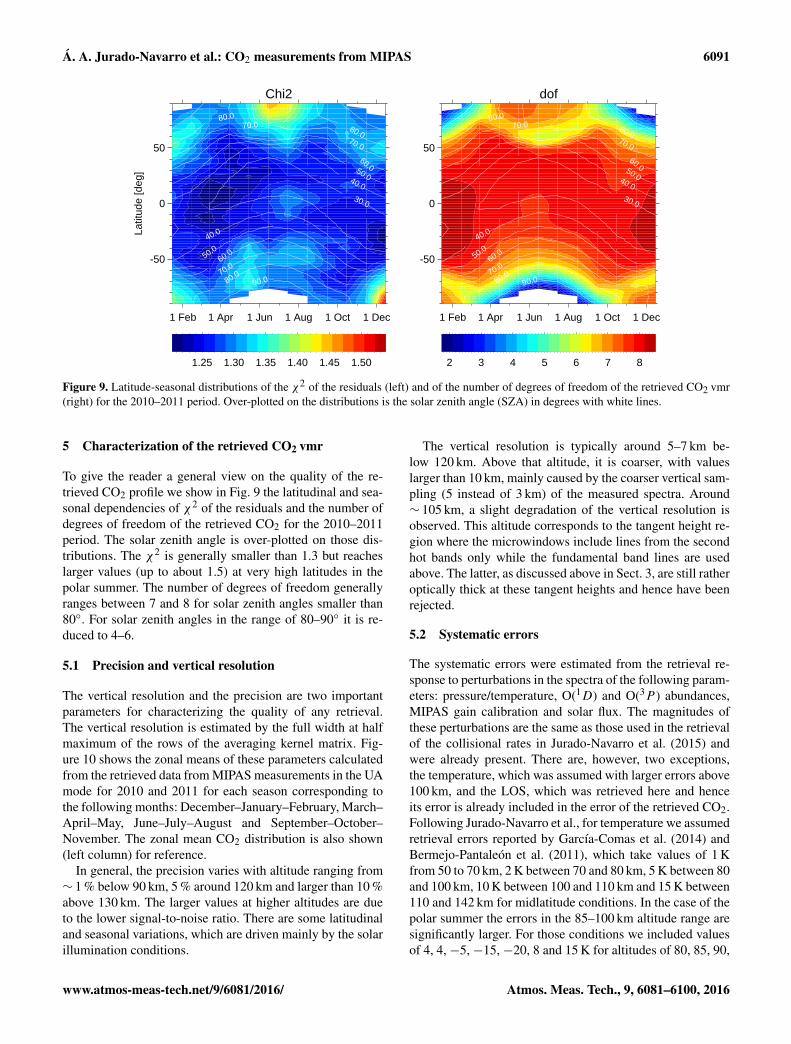
Figure 9. Latitude-seasonal distributions of the χ2 of the residuals (left) and of the number of degrees of freedom of the retrieved CO2 vmr(right) for the 2010–2011 period. Over-plotted on the distributions is the solar zenith angle (SZA) in degrees with white lines.

5 Characterization of the retrieved CO2 vmr

To give the reader a general view on the quality of the re-trieved CO2 profile we show in Fig. 9 the latitudinal and sea-sonal dependencies of χ2 of the residuals and the number ofdegrees of freedom of the retrieved CO2 for the 2010–2011period. The solar zenith angle is over-plotted on those dis-tributions. The χ2 is generally smaller than 1.3 but reacheslarger values (up to about 1.5) at very high latitudes in thepolar summer. The number of degrees of freedom generallyranges between 7 and 8 for solar zenith angles smaller than80◦. For solar zenith angles in the range of 80–90◦ it is re-duced to 4–6.

5.1 Precision and vertical resolution

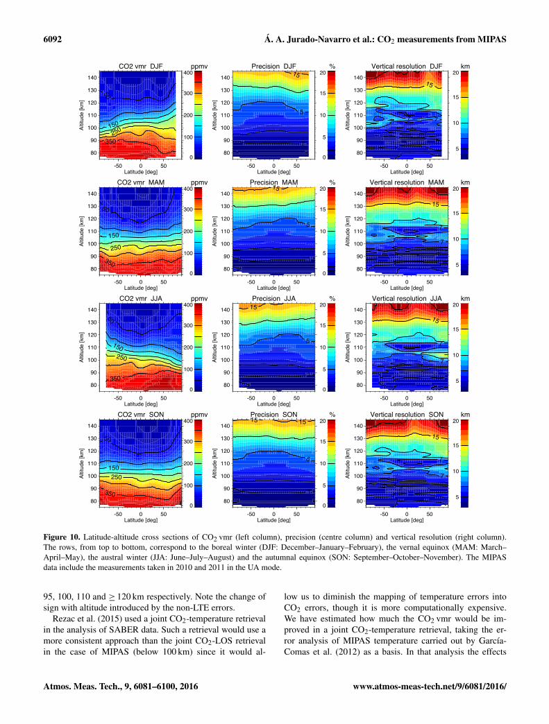
The vertical resolution and the precision are two importantparameters for characterizing the quality of any retrieval.The vertical resolution is estimated by the full width at halfmaximum of the rows of the averaging kernel matrix. Fig-ure 10 shows the zonal means of these parameters calculatedfrom the retrieved data from MIPAS measurements in the UAmode for 2010 and 2011 for each season corresponding tothe following months: December–January–February, March–April–May, June–July–August and September–October–November. The zonal mean CO2 distribution is also shown(left column) for reference.

In general, the precision varies with altitude ranging from∼ 1 % below 90 km, 5 % around 120 km and larger than 10 %above 130 km. The larger values at higher altitudes are dueto the lower signal-to-noise ratio. There are some latitudinaland seasonal variations, which are driven mainly by the solarillumination conditions.

The vertical resolution is typically around 5–7 km be-low 120 km. Above that altitude, it is coarser, with valueslarger than 10 km, mainly caused by the coarser vertical sam-pling (5 instead of 3 km) of the measured spectra. Around∼ 105 km, a slight degradation of the vertical resolution isobserved. This altitude corresponds to the tangent height re-gion where the microwindows include lines from the secondhot bands only while the fundamental band lines are usedabove. The latter, as discussed above in Sect. 3, are still ratheroptically thick at these tangent heights and hence have beenrejected.

5.2 Systematic errors

The systematic errors were estimated from the retrieval re-sponse to perturbations in the spectra of the following param-eters: pressure/temperature, O(1D) and O(3P ) abundances,MIPAS gain calibration and solar flux. The magnitudes ofthese perturbations are the same as those used in the retrievalof the collisional rates in Jurado-Navarro et al. (2015) andwere already present. There are, however, two exceptions,the temperature, which was assumed with larger errors above100 km, and the LOS, which was retrieved here and henceits error is already included in the error of the retrieved CO2.Following Jurado-Navarro et al., for temperature we assumedretrieval errors reported by García-Comas et al. (2014) andBermejo-Pantaleón et al. (2011), which take values of 1 Kfrom 50 to 70 km, 2 K between 70 and 80 km, 5 K between 80and 100 km, 10 K between 100 and 110 km and 15 K between110 and 142 km for midlatitude conditions. In the case of thepolar summer the errors in the 85–100 km altitude range aresignificantly larger. For those conditions we included valuesof 4, 4, −5, −15, −20, 8 and 15 K for altitudes of 80, 85, 90,



-50 0 50Latitude [deg]

80

90

100

110

120

130

140A

ltitu

de [k

m]

CO2 vmr DJF

50

150

250

350

ppmv

0

100

200

300

400


80

90

100

110

120

130

140

Alti

tude

[km

]

Precision DJF

1

5

15 %

0

5

10

15

20


80

90

100

110

120

130

140

Alti

tude

[km

]

Vertical resolution DJF

77

15

km

5

10

15

20


80

90

100

110

120

130

140

Alti

tude

[km

]

CO2 vmr MAM

50

150

250

350

ppmv

0

100

200

300

400


80

90

100

110

120

130

140

Alti

tude

[km

]

Precision MAM

1

5

15 %

0

5

10

15

20


80

90

100

110

120

130

140

Alti

tude

[km

]

Vertical resolution MAM

7

7

15

km

5

10

15

20


80

90

100

110

120

130

140

Alti

tude

[km

]

CO2 vmr JJA

50

150250

350

ppmv

0

100

200

300

400


80

90

100

110

120

130

140

Alti

tude

[km

]

Precision JJA

1

5

15 %

0

5

10

15

20


80

90

100

110

120

130

140

Alti

tude

[km

]

Vertical resolution JJA

7

7

15

km

5

10

15

20


80

90

100

110

120

130

140

Alti

tude

[km

]

CO2 vmr SON

50

150250

350

ppmv

0

100

200

300

400


80

90

100

110

120

130

140

Alti

tude

[km

]

Precision SON

1

5

1515 %

0

5

10

15

20


80

90

100

110

120

130

140

Alti

tude

[km

]

Vertical resolution SON

7

7

15

km

5

10

15

20

Figure 10. Latitude-altitude cross sections of CO2 vmr (left column), precision (centre column) and vertical resolution (right column).The rows, from top to bottom, correspond to the boreal winter (DJF: December–January–February), the vernal equinox (MAM: March–April–May), the austral winter (JJA: June–July–August) and the autumnal equinox (SON: September–October–November). The MIPASdata include the measurements taken in 2010 and 2011 in the UA mode.

95, 100, 110 and ≥ 120 km respectively. Note the change ofsign with altitude introduced by the non-LTE errors.

Rezac et al. (2015) used a joint CO2-temperature retrievalin the analysis of SABER data. Such a retrieval would use amore consistent approach than the joint CO2-LOS retrievalin the case of MIPAS (below 100 km) since it would al-

low us to diminish the mapping of temperature errors intoCO2 errors, though it is more computationally expensive.We have estimated how much the CO2 vmr would be im-proved in a joint CO2-temperature retrieval, taking the er-ror analysis of MIPAS temperature carried out by García-Comas et al. (2012) as a basis. In that analysis the effects



of the hydrostatical adjustment of pressure due to the tem-perature changes were taken into account. We only considerthe altitudes below 100 km, where the temperature retrievedfrom the CO2 15 µm MIPAS spectra is used, and hence theCO2 vmr is needed. In the best case, assuming the CO2 vmris free of errors in the temperature retrieval, the temperatureerror would be improved for midlatitude conditions in about1 K at 85 km and 0.8 K and 0.1 K at 90 and 100 km respec-tively (see Table 2 in García-Comas et al., 2012). For polarsummer conditions, the reduction is smaller, 0.7 K at 85 kmand 0.1 K at 90–100 km, because non-LTE errors are morerelevant. These errors would improve the retrieved CO2 er-ror in 0.7 % at 85 km and only 0.1 % at 90–100 km for themidlatitudes. For polar summer latitudes, the improvementswould be even smaller because, at 85 km, the temperatureerror contribution to the CO2 error budget is smaller (see Ta-ble 1) and, at higher altitudes, because the improvement inthe temperature error is not significant. Hence, we expect thatthe joint CO2-temperature retrieval would not significantlyimprove the accuracy of the retrieved CO2 vmr.

Regarding the error introduced by the absolute pointing(the error due to the relative pointing, i.e. between adja-cent scans, is already included in the retrieval error since itis jointly retrieved with the CO2 vmr), von Clarmann et al.(2003) estimated the total systematic error in the retrieved ab-solute pointing from 15 µm to be less than 200 m. This errorintroduces an error in the CO2 vmr that is smaller than 1 %below 90 km, between 1 and 1.5 % at 90–120 km and smallerthan 1 % above that altitude. Overall this error is negligiblein comparison with the other error sources (see Table 1).

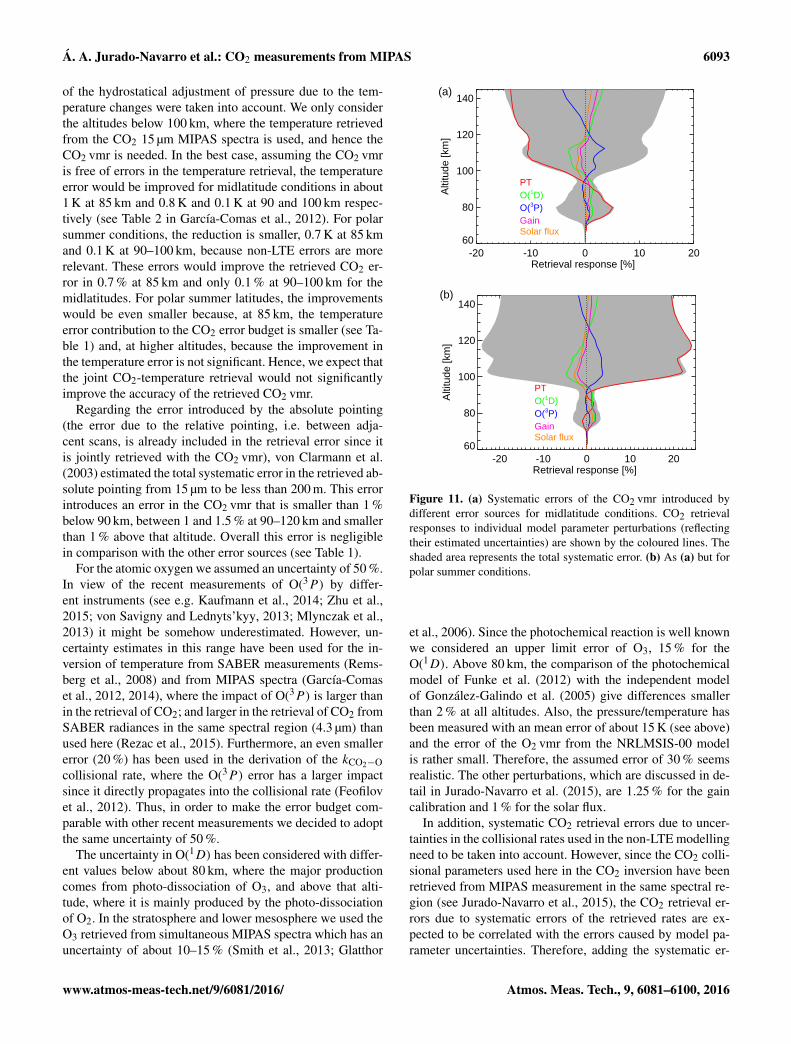
For the atomic oxygen we assumed an uncertainty of 50 %.In view of the recent measurements of O(3P) by differ-ent instruments (see e.g. Kaufmann et al., 2014; Zhu et al.,2015; von Savigny and Lednyts’kyy, 2013; Mlynczak et al.,2013) it might be somehow underestimated. However, un-certainty estimates in this range have been used for the in-version of temperature from SABER measurements (Rems-berg et al., 2008) and from MIPAS spectra (García-Comaset al., 2012, 2014), where the impact of O(3P) is larger thanin the retrieval of CO2; and larger in the retrieval of CO2 fromSABER radiances in the same spectral region (4.3 µm) thanused here (Rezac et al., 2015). Furthermore, an even smallererror (20 %) has been used in the derivation of the kCO2−Ocollisional rate, where the O(3P) error has a larger impactsince it directly propagates into the collisional rate (Feofilovet al., 2012). Thus, in order to make the error budget com-parable with other recent measurements we decided to adoptthe same uncertainty of 50 %.

The uncertainty in O(1D) has been considered with differ-ent values below about 80 km, where the major productioncomes from photo-dissociation of O3, and above that alti-tude, where it is mainly produced by the photo-dissociationof O2. In the stratosphere and lower mesosphere we used theO3 retrieved from simultaneous MIPAS spectra which has anuncertainty of about 10–15 % (Smith et al., 2013; Glatthor

-20 -10 0 10 20Retrieval response [%]

60

80

100

120

140

Alti

tude

[km

]

PTO(1D)O(3P)GainSolar flux

-20 -10 0 10 20Retrieval response [%]

60

80

100

120

140

Alti

tude

[km

]

PTO(1D)O(3P)GainSolar flux

(a)

(b)

Figure 11. (a) Systematic errors of the CO2 vmr introduced bydifferent error sources for midlatitude conditions. CO2 retrievalresponses to individual model parameter perturbations (reflectingtheir estimated uncertainties) are shown by the coloured lines. Theshaded area represents the total systematic error. (b) As (a) but forpolar summer conditions.

et al., 2006). Since the photochemical reaction is well knownwe considered an upper limit error of O3, 15 % for theO(1D). Above 80 km, the comparison of the photochemicalmodel of Funke et al. (2012) with the independent modelof González-Galindo et al. (2005) give differences smallerthan 2 % at all altitudes. Also, the pressure/temperature hasbeen measured with an mean error of about 15 K (see above)and the error of the O2 vmr from the NRLMSIS-00 modelis rather small. Therefore, the assumed error of 30 % seemsrealistic. The other perturbations, which are discussed in de-tail in Jurado-Navarro et al. (2015), are 1.25 % for the gaincalibration and 1 % for the solar flux.

In addition, systematic CO2 retrieval errors due to uncer-tainties in the collisional rates used in the non-LTE modellingneed to be taken into account. However, since the CO2 colli-sional parameters used here in the CO2 inversion have beenretrieved from MIPAS measurement in the same spectral re-gion (see Jurado-Navarro et al., 2015), the CO2 retrieval er-rors due to systematic errors of the retrieved rates are ex-pected to be correlated with the errors caused by model pa-rameter uncertainties. Therefore, adding the systematic er-



0 5 10 15 20 25Total systematic error [%]

60

80

100

120

140

Alti

tude

[km

]

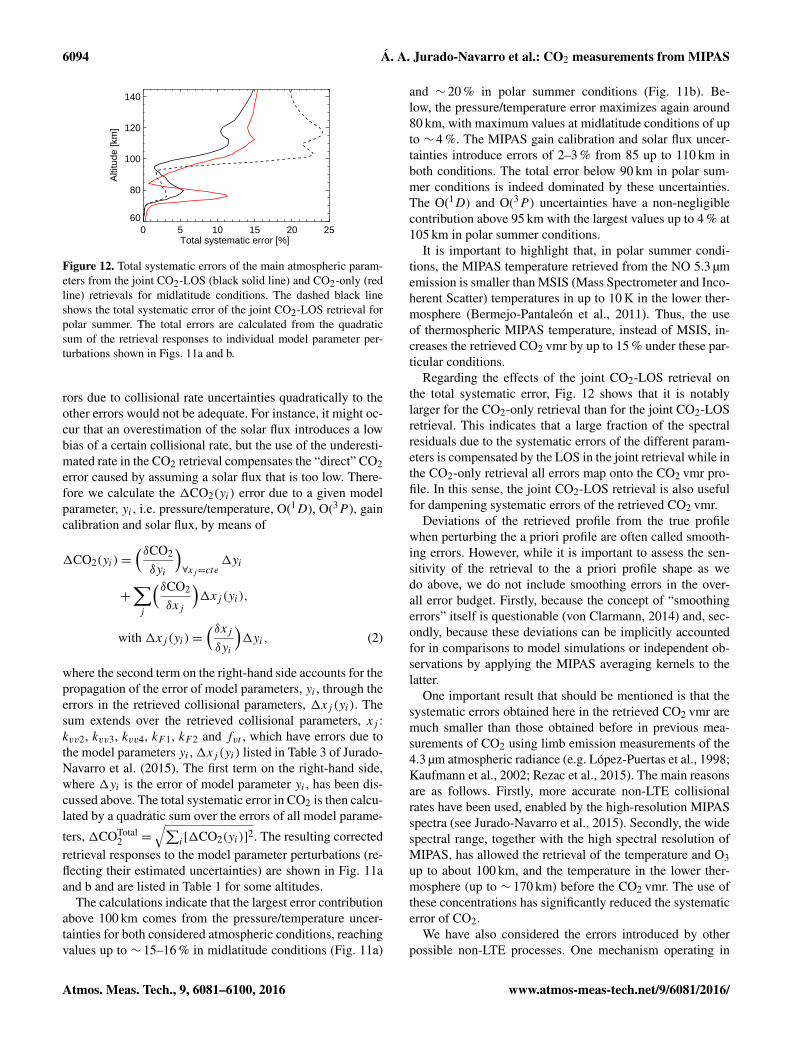
Figure 12. Total systematic errors of the main atmospheric param-eters from the joint CO2-LOS (black solid line) and CO2-only (redline) retrievals for midlatitude conditions. The dashed black lineshows the total systematic error of the joint CO2-LOS retrieval forpolar summer. The total errors are calculated from the quadraticsum of the retrieval responses to individual model parameter per-turbations shown in Figs. 11a and b.

rors due to collisional rate uncertainties quadratically to theother errors would not be adequate. For instance, it might oc-cur that an overestimation of the solar flux introduces a lowbias of a certain collisional rate, but the use of the underesti-mated rate in the CO2 retrieval compensates the “direct” CO2error caused by assuming a solar flux that is too low. There-fore we calculate the 1CO2(yi) error due to a given modelparameter, yi , i.e. pressure/temperature, O(1D), O(3P ), gaincalibration and solar flux, by means of

1CO2(yi)=(δCO2

δyi

)∀xj=cte

1yi

+

∑j

(δCO2

δxj

)1xj (yi),

with 1xj (yi)=(δxjδyi

)1yi, (2)

where the second term on the right-hand side accounts for thepropagation of the error of model parameters, yi , through theerrors in the retrieved collisional parameters, 1xj (yi). Thesum extends over the retrieved collisional parameters, xj :kvv2, kvv3, kvv4, kF1, kF2 and fvt , which have errors due tothe model parameters yi ,1xj (yi) listed in Table 3 of Jurado-Navarro et al. (2015). The first term on the right-hand side,where 1yi is the error of model parameter yi , has been dis-cussed above. The total systematic error in CO2 is then calcu-lated by a quadratic sum over the errors of all model parame-

ters, 1COTotal2 =

√∑i[1CO2(yi)]2. The resulting corrected

retrieval responses to the model parameter perturbations (re-flecting their estimated uncertainties) are shown in Fig. 11aand b and are listed in Table 1 for some altitudes.

The calculations indicate that the largest error contributionabove 100 km comes from the pressure/temperature uncer-tainties for both considered atmospheric conditions, reachingvalues up to ∼ 15–16 % in midlatitude conditions (Fig. 11a)

and ∼ 20 % in polar summer conditions (Fig. 11b). Be-low, the pressure/temperature error maximizes again around80 km, with maximum values at midlatitude conditions of upto ∼ 4 %. The MIPAS gain calibration and solar flux uncer-tainties introduce errors of 2–3 % from 85 up to 110 km inboth conditions. The total error below 90 km in polar sum-mer conditions is indeed dominated by these uncertainties.The O(1D) and O(3P) uncertainties have a non-negligiblecontribution above 95 km with the largest values up to 4 % at105 km in polar summer conditions.

It is important to highlight that, in polar summer condi-tions, the MIPAS temperature retrieved from the NO 5.3 µmemission is smaller than MSIS (Mass Spectrometer and Inco-herent Scatter) temperatures in up to 10 K in the lower ther-mosphere (Bermejo-Pantaleón et al., 2011). Thus, the useof thermospheric MIPAS temperature, instead of MSIS, in-creases the retrieved CO2 vmr by up to 15 % under these par-ticular conditions.

Regarding the effects of the joint CO2-LOS retrieval onthe total systematic error, Fig. 12 shows that it is notablylarger for the CO2-only retrieval than for the joint CO2-LOSretrieval. This indicates that a large fraction of the spectralresiduals due to the systematic errors of the different param-eters is compensated by the LOS in the joint retrieval while inthe CO2-only retrieval all errors map onto the CO2 vmr pro-file. In this sense, the joint CO2-LOS retrieval is also usefulfor dampening systematic errors of the retrieved CO2 vmr.

Deviations of the retrieved profile from the true profilewhen perturbing the a priori profile are often called smooth-ing errors. However, while it is important to assess the sen-sitivity of the retrieval to the a priori profile shape as wedo above, we do not include smoothing errors in the over-all error budget. Firstly, because the concept of “smoothingerrors” itself is questionable (von Clarmann, 2014) and, sec-ondly, because these deviations can be implicitly accountedfor in comparisons to model simulations or independent ob-servations by applying the MIPAS averaging kernels to thelatter.

One important result that should be mentioned is that thesystematic errors obtained here in the retrieved CO2 vmr aremuch smaller than those obtained before in previous mea-surements of CO2 using limb emission measurements of the4.3 µm atmospheric radiance (e.g. López-Puertas et al., 1998;Kaufmann et al., 2002; Rezac et al., 2015). The main reasonsare as follows. Firstly, more accurate non-LTE collisionalrates have been used, enabled by the high-resolution MIPASspectra (see Jurado-Navarro et al., 2015). Secondly, the widespectral range, together with the high spectral resolution ofMIPAS, has allowed the retrieval of the temperature and O3up to about 100 km, and the temperature in the lower ther-mosphere (up to ∼ 170 km) before the CO2 vmr. The use ofthese concentrations has significantly reduced the systematicerror of CO2.

We have also considered the errors introduced by otherpossible non-LTE processes. One mechanism operating in



Apr 2010

0 100 200 300 400 500CO2 volume mixing ratio (ppmv)

60

80

100

120

140

Alti

tude

(km

)

Dec 2010

0 100 200 300 400 500CO2 volume mixing ratio (ppmv)

60

80

100

120

140

Alti

tude

(km

)

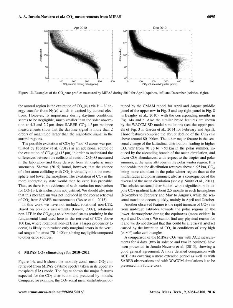
Figure 13. Examples of the CO2 vmr profiles measured by MIPAS during 2010 for April (equinox, left) and December (solstice, right).

the auroral region is the excitation of CO2(v3) via V −V en-ergy transfer from N2(v) which is excited by auroral elec-trons. However, its importance during daytime conditionsseems to be negligible, much smaller than the solar absorp-tion at 4.3 and 2.7 µm since SABER CO2 4.3 µm radiancemeasurements show that the daytime signal is more than 2orders of magnitude larger than the night-time signal in theauroral regions.

The possible excitation of CO2 by “hot” O atoms was pos-tulated by Feofilov et al. (2012) as an additional source ofthe excitation of CO2(v2) (15 µm) in order to understand thedifferences between the collisional rates of CO2-O measuredin the laboratory and those derived from atmospheric mea-surements. Sharma (2015) found, however, that the chanceof a hot atom colliding with CO2 is virtually nil in the meso-sphere and lower thermosphere. The excitation of CO2 in themore energetic v3 state would then be even less probable.Thus, as there is no evidence of such excitation mechanismfor CO2(v3), its inclusion is not justified. We should also notethat this mechanism was not included in the recent retrievalof CO2 from SABER measurements (Rezac et al., 2015).

In this work we have not included rotational non-LTE.Based on previous assessments (Gusev, 2002), rotationalnon-LTE in the CO2(v3) ro-vibrational states (emitting in thefundamental band used here in the retrieval of CO2 above100 km, where rotational non-LTE has a larger propensity tooccur) is likely to introduce only marginal errors in the verti-cal range of interest (70–140 km), being negligible comparedto other error sources.

6 MIPAS CO2 climatology for 2010–2011

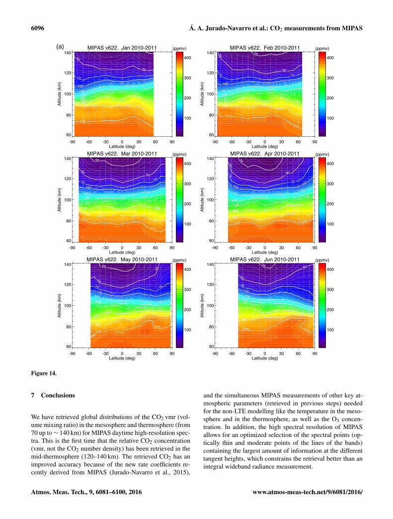
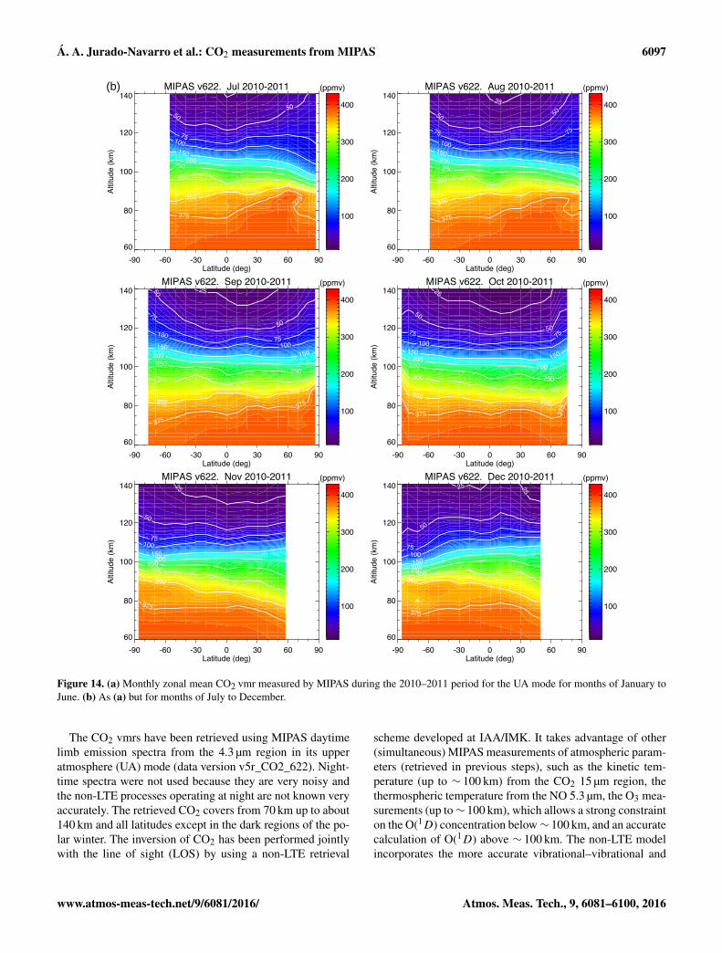
Figure 14a and b shows the monthly zonal mean CO2 vmrretrieved from MIPAS daytime spectra taken in its upper at-mosphere (UA) mode. The figure shows the major featuresexpected for the CO2 distribution and predicted by models.Compare, for example, the CO2 zonal mean distributions ob-

tained by the CMAM model for April and August (middlepanel of the upper row in Fig. 3 and top-right panel in Fig. 8in Beagley et al., 2010), with the corresponding months inFig. 14a and b. Also the similar broad features are shownby the WACCM-SD model simulations (see the upper pan-els of Fig. 3 in Garcia et al., 2014 for February and April).Those features comprise the abrupt decline of the CO2 vmrabove around 80–90 km. The other major feature is the sea-sonal change of the latitudinal distribution, leading to higherCO2 vmr from 70 up to ∼ 95 km in the polar summer, in-duced by the ascending branch of the mean circulation, andlower CO2 abundances, with respect to the tropics and polarsummer, at the same altitudes in the polar winter region. It isnoticeable that the distribution reverses above ∼ 95 km, CO2being more abundant in the polar winter region than at themidlatitudes and polar summer; also as a consequence of thereversal of the mean circulation (see e.g. Smith et al., 2011).The solstice seasonal distribution, with a significant pole-to-pole CO2 gradient lasts about 2.5 months in each hemisphere(November to February and May to August), while the sea-sonal transition occurs quickly, mainly in April and October.

Another observed feature is the rapid increase of CO2 vmrfrom mid-high latitudes towards the polar regions in thelower thermosphere during the equinoxes (more evident inApril and October). We cannot find any physical reason forit and we do not discard that this could be a retrieval artefactcaused by the inversion of CO2 in conditions of very high(> 80◦) solar zenith angles.

A comparison of the MIPAS CO2 vmr with ACE measure-ments for 4 days (two in solstice and two in equinox) havebeen presented in Jurado-Navarro et al. (2015), showing agood general agreement. A more detailed comparison withACE data covering a more extended period as well as withSABER observations and with WACCM simulations is to bepresented in a future work.



MIPAS v622. Jan 2010-2011

-90 -60 -30 0 30 60 90Latitude (deg)

60

80

100

120

140A

ltitu

de (

km)

50

50

75

100

150200

250300

350

375

(ppmv)

100

200

300

400

MIPAS v622. Feb 2010-2011

-90 -60 -30 0 30 60 90Latitude (deg)

60

80

100

120

140

Alti

tude

(km

)

2550

50

75 75

100

150200250

250

300 300350

375

375

(ppmv)

100

200

300

400

MIPAS v622. Mar 2010-2011

-90 -60 -30 0 30 60 90Latitude (deg)

60

80

100

120

140

Alti

tude

(km

)

25

50

50

75 75

100

150

200

250

300 300350

350375

375

(ppmv)

100

200

300

400

MIPAS v622. Apr 2010-2011

-90 -60 -30 0 30 60 90Latitude (deg)

60

80

100

120

140

Alti

tude

(km

)

25

50

5075

75100 100

150150

200

250

250

300

350

375 375

(ppmv)

100

200

300

400

MIPAS v622. May 2010-2011

-90 -60 -30 0 30 60 90Latitude (deg)

60

80

100

120

140

Alti

tude

(km

)

25

50

50

75 75100

150200250

300

350

375375

(ppmv)

100

200

300

400

MIPAS v622. Jun 2010-2011

-90 -60 -30 0 30 60 90Latitude (deg)

60

80

100

120

140

Alti

tude

(km

)

25

50

50

75100150

200250

300

350

375 375

(ppmv)

100

200

300

400

(a)

Figure 14.

7 Conclusions

We have retrieved global distributions of the CO2 vmr (vol-ume mixing ratio) in the mesosphere and thermosphere (from70 up to∼ 140 km) for MIPAS daytime high-resolution spec-tra. This is the first time that the relative CO2 concentration(vmr, not the CO2 number density) has been retrieved in themid-thermosphere (120–140 km). The retrieved CO2 has animproved accuracy because of the new rate coefficients re-cently derived from MIPAS (Jurado-Navarro et al., 2015),

and the simultaneous MIPAS measurements of other key at-mospheric parameters (retrieved in previous steps) neededfor the non-LTE modelling like the temperature in the meso-sphere and in the thermosphere, as well as the O3 concen-tration. In addition, the high spectral resolution of MIPASallows for an optimized selection of the spectral points (op-tically thin and moderate points of the lines of the bands)containing the largest amount of information at the differenttangent heights, which constrains the retrieval better than anintegral wideband radiance measurement.



MIPAS v622. Jul 2010-2011

-90 -60 -30 0 30 60 90Latitude (deg)

60

80

100

120

140

Alti

tude

(km

)50

50

75100150

200250

300

350

375

375

(ppmv)

100

200

300

400

MIPAS v622. Aug 2010-2011

-90 -60 -30 0 30 60 90Latitude (deg)

60

80

100

120

140

Alti

tude

(km

)

25

50 50

75 75

100150200250

300

350

375

(ppmv)

100

200

300

400

MIPAS v622. Sep 2010-2011

-90 -60 -30 0 30 60 90Latitude (deg)

60

80

100

120

140

Alti

tude

(km

)

2550

50

75

75100

100150150200

250250

300

350

350

375

375

(ppmv)

100

200

300

400

MIPAS v622. Oct 2010-2011

-90 -60 -30 0 30 60 90Latitude (deg)

60

80

100

120

140

Alti

tude

(km

)

25

50

5075 75

100150

150200

200250

250300

300350

350

375 375

(ppmv)

100

200

300

400

MIPAS v622. Nov 2010-2011

-90 -60 -30 0 30 60 90Latitude (deg)

60

80

100

120

140

Alti

tude

(km

)

25

50

75100

150200

250300

350

375

(ppmv)

100

200

300

400

MIPAS v622. Dec 2010-2011

-90 -60 -30 0 30 60 90Latitude (deg)

60

80

100

120

140

Alti

tude

(km

)

25 25

50

75100150200250

300350

375

(ppmv)

100

200

300

400

(b)

Figure 14. (a) Monthly zonal mean CO2 vmr measured by MIPAS during the 2010–2011 period for the UA mode for months of January toJune. (b) As (a) but for months of July to December.

The CO2 vmrs have been retrieved using MIPAS daytimelimb emission spectra from the 4.3 µm region in its upperatmosphere (UA) mode (data version v5r_CO2_622). Night-time spectra were not used because they are very noisy andthe non-LTE processes operating at night are not known veryaccurately. The retrieved CO2 covers from 70 km up to about140 km and all latitudes except in the dark regions of the po-lar winter. The inversion of CO2 has been performed jointlywith the line of sight (LOS) by using a non-LTE retrieval

scheme developed at IAA/IMK. It takes advantage of other(simultaneous) MIPAS measurements of atmospheric param-eters (retrieved in previous steps), such as the kinetic tem-perature (up to ∼ 100 km) from the CO2 15 µm region, thethermospheric temperature from the NO 5.3 µm, the O3 mea-surements (up to∼ 100 km), which allows a strong constrainton the O(1D) concentration below∼ 100 km, and an accuratecalculation of O(1D) above ∼ 100 km. The non-LTE modelincorporates the more accurate vibrational–vibrational and



vibrational–translational collisional rates retrieved from theMIPAS spectra.

The precision of the retrieved CO2 vmr profiles varies withaltitude, ranging from ∼ 1 % below 90 km to 5 % around120 km and larger than 10 % above 130 km. The larger valuesat higher altitudes are due to the lower signal-to-noise ratio.There are very few latitudinal and seasonal variations of theprecision, which are mainly driven by the solar illuminationconditions. The retrieved CO2 profiles have a vertical reso-lution of about 5–7 below 120 km and between 10 and 20 at120–140 km.

Retrieval simulations performed with synthetic spectrahave demonstrated that the developed CO2-LOS joint re-trieval allows for a retrieval of the CO2 profile in the 70–140 km range with high accuracy. The use of strongly per-turbed a priori CO2 and LOS information results in verysmall different between the true and the retrieved profiles,generally smaller than 2–3 % in the midlatitudes and smallerthan 2 % (except near 95–110 km where it ranges at 2–4 %)for polar summer conditions. We have also proven that thealgorithm is capable of retrieving unusual CO2 profiles suchas those showing a low vmr between 70 and 85 km and a pro-nounced peak near 90 km, and also CO2 profiles affected bywave propagation. The retrieval scheme clearly discriminatesthe information of CO2 concentration from the LOS. Themapping of typical CO2 a priori uncertainties on the LOSis very small (less than 20 m), and a deviation in the a pri-ori LOS profile of 200 m introduces a change in the retrievedCO2 profile smaller than 1–2 %. We have also found that thesystematic errors are significantly reduced when using theCO2-LOS joint retrieval instead of the CO2-only scheme.

The major systematic error source is the uncertainty ofthe pressure/temperature profiles, retrieved also from MI-PAS spectra, near 15 µm below 100 km (García-Comas et al.,2014) and from 5.3 µm above 100 km Bermejo-Pantaleónet al. (2011). They can induce a systematic error at midlat-itude conditions of up to 15 % above 100 km (20 % for polarsummer conditions) and of ∼ 5 % around 80 km. The sys-tematic errors due to uncertainties of the O(1D) and O(3P )profiles are within 3–4 % in the 100–120 km region. The er-rors due to uncertainties in the gain calibration and in thesolar flux at 4.3 and 2.7 µm are within ∼ 2 % at all altitudes.

The most important features observed on the retrievedCO2 can be summarized as follows:

– The retrieved CO2 shows the major general featuresexpected and predicted by models: the abrupt declineof the CO2 vmr above 80–90 km, caused by the pre-dominance of the molecular diffusion and the seasonalchange of the latitudinal distribution. The latter is re-flected by higher CO2 abundances in polar summerfrom 70 km up to ∼ 95 km and lower CO2 vmr in thepolar winter, both induced by the ascending and de-scending branches of the mean circulation respectively.Above∼ 95 km, CO2 is more abundant in the polar win-

ter than at the midlatitudes and polar summer regions,caused by the reversal of the mean circulation in thataltitude region.

– The solstice seasonal distribution, with a significantpole-to-pole CO2 gradient lasts about 2.5 months ineach hemisphere (November to February and May toAugust), while the seasonal transition occurs quickly,mainly in April and October.

8 Data availability

The retrieved CO2 volume mixing ratio data versionv5r_CO2_622 will be made available at the IMK-IAA MI-PAS data set website: https://www.imk-asf.kit.edu/english/308.php, once the final processing is finished.

The Supplement related to this article is available onlineat doi:10.5194/amt-9-6081-2016-supplement.

Acknowledgements. The IAA team was supported by the SpanishMCINN under grant ESP2014-54362-P and EC FEDER funds.Maya García-Comas was financially supported by the Ministry ofEconomy and Competitiveness (MINECO) through its “Ramóny Cajal” subprogramme. The authors acknowledge ESA forproviding MIPAS L1b spectra.

Edited by: S. KirkwoodReviewed by: A. Feofilov and one anonymous referee

References

Beagley, S. R., Boone, C. D., Fomichev, V. I., Jin, J. J., Semeniuk,K., McConnell, J. C., and Bernath, P. F.: First multi-year occul-tation observations of CO2 in the MLT by ACE satellite: obser-vations and analysis using the extended CMAM, Atmos. Chem.Phys., 10, 1133–1153, doi:10.5194/acp-10-1133-2010, 2010.

Bermejo-Pantaleón, D., Funke, B., Lopez-Puertas, M., García-Comas, M., Stiller, G. P., von Clarmann, T., Linden, A.,Grabowski, U., Höpfner, M., Kiefer, M., Glatthor, N., Kellmann,S., and Lu, G.: Global Observations of Thermospheric Tempera-ture and Nitric Oxide from MIPAS spectra at 5.3 µm, J. Geophys.Res., 116, A10313, doi:10.1029/2011JA016752, 2011.

De Laurentis, M.: Planning of MIPAS new special modes January2005 Campaign, Tech. rep., ESA Technical Note, ENVI-SPPA-EOPG-TN-05-0002, 2005.

Feofilov, A. G., Kutepov, A. A., She, C.-Y., Smith, A. K., Pesnell,W. D., and Goldberg, R. A.: CO2(v2)-O quenching rate coeffi-cient derived from coincidental SABER/TIMED and Fort Collinslidar observations of the mesosphere and lower thermosphere,Atmos. Chem. Phys., 12, 9013–9023, doi:10.5194/acp-12-9013-2012, 2012.


https://www.imk-asf.kit.edu/english/308.php

https://www.imk-asf.kit.edu/english/308.php

http://dx.doi.org/10.5194/amt-9-6081-2016-supplement

http://dx.doi.org/10.5194/acp-10-1133-2010

http://dx.doi.org/10.1029/2011JA016752




Fischer, H., Birk, M., Blom, C., Carli, B., Carlotti, M., von Clar-mann, T., Delbouille, L., Dudhia, A., Ehhalt, D., Endemann, M.,Flaud, J. M., Gessner, R., Kleinert, A., Koopman, R., Langen, J.,López-Puertas, M., Mosner, P., Nett, H., Oelhaf, H., Perron, G.,Remedios, J., Ridolfi, M., Stiller, G., and Zander, R.: MIPAS: aninstrument for atmospheric and climate research, Atmos. Chem.Phys., 8, 2151–2188, doi:10.5194/acp-8-2151-2008, 2008.

Foucher, P. Y., Chédin, A., Armante, R., Boone, C., Crevoisier,C., and Bernath, P.: Carbon dioxide atmospheric vertical pro-files retrieved from space observation using ACE-FTS solaroccultation instrument, Atmos. Chem. Phys., 11, 2455–2470,doi:10.5194/acp-11-2455-2011, 2011.

Funke, B., López-Puertas, M., Stiller, G. P., von Clarmann, T., andHöpfner, M.: A new non–LTE Retrieval Method for AtmosphericParameters From MIPAS–ENVISAT Emission Spectra, Adv.Space Res., 27, 1099–1104, doi:10.1016/S0273-1177(01)00169-7, 2001.

Funke, B., López-Puertas, M., García-Comas, M., Stiller, G. P., vonClarmann, T., Höpfner, M., Glatthor, N., Grabowski, U., Kell-mann, S., and Linden, A.: Carbon monoxide distributions fromthe upper troposphere to the mesosphere inferred from 4.7 µmnon-local thermal equilibrium emissions measured by MIPAS onEnvisat, Atmos. Chem. Phys., 9, 2387–2411, doi:10.5194/acp-9-2387-2009, 2009.

Funke, B., López-Puertas, M., García-Comas, M., Kaufmann, M.,Höpfner, M., and Stiller, G. P.: GRANADA: a Generic RAdiativetraNsfer AnD non-LTE population Algorithm, J. Quant. Spec-trosc. Ra., 113, 1771–1817, doi:10.1016/j.jqsrt.2012.05.001,2012.

Garcia, R. R., López-Puertas, M., Funke, B., Marsh, D. R.,Kinnison, D. E., Smith, A. K., and González-Galindo, F.:On the distribution of CO2 and CO in the mesosphere andlower thermosphere, J. Geophys. Res.-Atmos., 119, 5700–5718,doi:10.1002/2013JD021208, 2014.

García-Comas, M., Funke, B., López-Puertas, M., Bermejo-Pantaleón, D., Glatthor, N., von Clarmann, T., Stiller, G.,Grabowski, U., Boone, C. D., French, W. J. R., Leblanc, T.,López-González, M. J., and Schwartz, M. J.: On the quality ofMIPAS kinetic temperature in the middle atmosphere, Atmos.Chem. Phys., 12, 6009–6039, doi:10.5194/acp-12-6009-2012,2012.

García-Comas, M., Funke, B., Gardini, A., López-Puertas, M.,Jurado-Navarro, A., von Clarmann, T., Stiller, G., Kiefer, M.,Boone, C. D., Leblanc, T., Marshall, B. T., Schwartz, M. J.,and Sheese, P. E.: MIPAS temperature from the stratosphere tothe lower thermosphere: Comparison of vM21 with ACE-FTS,MLS, OSIRIS, SABER, SOFIE and lidar measurements, At-mos. Meas. Tech., 7, 3633–3651, doi:10.5194/amt-7-3633-2014,2014.

Gil-López, S., López-Puertas, M., Kaufmann, M., Funke, B.,García-Comas, M., Koukouli, M. E., Glatthor, N., Grabowski,U., Höpfner, Stiller, G. P., and von Clarmann, T.: Retrievalof stratospheric and mesospheric O3 from high resolution MI-PAS spectra at 15 and 10 µm, Adv. Space Res., 36, 943–951,doi:10.1016/j.asr.2005.05.123, 2005.

Glatthor, N., von Clarmann, T., Fischer, H., Funke, B., Gil-López, S., Grabowski, U., Höpfner, M., Kellmann, S., Lin-den, A., López-Puertas, M., Mengistu Tsidu, G., Milz, M.,Steck, T., Stiller, G. P., and Wang, D.-Y.: Retrieval of strato-

spheric ozone profiles from MIPAS/ENVISAT limb emissionspectra: a sensitivity study, Atmos. Chem. Phys., 6, 2767–2781,doi:10.5194/acp-6-2767-2006, 2006.

González-Galindo, F., López-Valverde, M. A., Angelats i Coll, M.,and Forget, F.: Extension of a Martian general circulation modelto thermospheric altitudes: UV heating and photochemical mod-els, J. Geophys. Res., 110, 09008, doi:10.1029/2004JE002312,2005.

Gusev, O.: Non-LTE diagnostics of the infrared observations ofthe planetary atmosphere, PhD thesis, München Universität, Mu-nich, 2002.

Jurado-Navarro, Á. A., López-Puertas, M., Funke, B., García-Comas, M., Gardini, A., Stiller, G. P., and Clarmann,T. V.: Vibrational-vibrational and vibrational-thermal energytransfers of CO2 with N2 from MIPAS high-resolutionlimb spectra, J. Geophys. Res.-Atmos., 120, 8002–8022,doi:10.1002/2015JD023429, 2015.

Kaufmann, M., Gusev, O. A., Grossmann, K. U., Roble, R. G.,Hagan, M. E., Hartsough, C., and Kutepov, A. A.: The ver-tical and horizontal distribution of CO2 densities in the up-per mesosphere and lower thermosphere as measured byCRISTA, J. Geophys. Res.-Atmos., 107, CRI 10-1–CRI 10-19,doi:10.1029/2001JD000704, 2002.

Kaufmann, M., Zhu, Y., Ern, M., and Riese, M.: Global distribu-tion of atomic oxygen in the mesopause region as derived fromSCIAMACHY O(1S) green line measurements, Geophys. Res.Lett., 41, 6274–6280, 2014.

Lean, J., Rottman, G., Harder, J., and Kopp, G.: SORCE Contribu-tions to New Understanding of Global Change and Solar Vari-ability, Solar Phys., 230, 27–53, 2005.

Levenberg, K.: A method for the solution of certain non–linearproblems in least squares, Quart. Appl. Math., 2, 164–168, 1944.

López-Puertas, M. and Taylor, F. W.: Non-LTE radiative transfer inthe Atmosphere, World Scientific Pub., Singapore, 2001.

López-Puertas, M., Zaragoza, G., López-Valverde, M. Á., and Tay-lor, F. W.: Non local thermodynamic equilibrium (LTE) atmo-spheric limb emission at 4.6 µm 2. An analysis of the daytimewideband radiances as measured by UARS improved strato-spheric and mesospheric sounder, J. Geophys. Res., 103, 8515–8530, 1998.

López-Puertas, M., López-Valverde, M. Á., Garcia, R. R., andRoble, R. G.: A review of CO2 and CO abundances in the mid-dle atmosphere, in: Atmospheric Science Across the Stratopause,edited by: Siskind, D. E., Eckermann, S. D., and Summers, M. E.,Geophysical Monograph Series, 123, 83 pp., American Geophys-ical Union, 2000.

Lu, H. C., Chen, H. K., Chen, H. F., Cheng, B. M., and Ogilvie, J. F.:Absorption cross section of molecular oxygen in the transitionE36−u v= 0–X36−g v =0 at 38 K, Astron. Astrophys., 520, A19,doi:10.1051/0004-6361/201013998, 2010.

Marquardt, D. W.: An algorithm for least–squares estimation ofnonlinear parameters, J. Soc. Indust. Appl. Math., 11, 431–441,1963.

Mlynczak, M. G., Hunt, L. A., Mast, J. C., Thomas Marshall, B.,Russell, J., Smith, A. K., Siskind, D. E., Yee, J.-H., Mertens,C. J., Javier Martin-Torres, F., Earl Thompson, R., Drob, D. P.,and Gordley, L. L.: Atomic oxygen in the mesosphere and lowerthermosphere derived from SABER: Algorithm theoretical basis




http://dx.doi.org/10.1016/S0273-1177(01)00169-7

http://dx.doi.org/10.1016/S0273-1177(01)00169-7



http://dx.doi.org/10.1016/j.jqsrt.2012.05.001

http://dx.doi.org/10.1002/2013JD021208


http://dx.doi.org/10.5194/amt-7-3633-2014

http://dx.doi.org/10.1016/j.asr.2005.05.123


http://dx.doi.org/10.1029/2004JE002312

http://dx.doi.org/10.1002/2015JD023429

http://dx.doi.org/10.1029/2001JD000704

http://dx.doi.org/10.1051/0004-6361/201013998


and measurement uncertainty, J. Geophys. Res., 118, 5724–5735,2013.

Norton, H. and Beer, R.: New apodizing functions for Fourier spec-trometry, J. Opt. Soc. Am., 66, 259–264, 1976.

Oelhaf, H.: MIPAS Mission Plan, ESA Technical Note ENVI-SPPA-EOPG-TN-07-0073, 2008.

Offermann, D. and Grossmann, K. U.: Thermospheric den-sity and composition as determined by a mass spectrome-ter with cryo ion source, J. Geophys. Res., 78, 8296–8304,doi:10.1029/JA078i034p08296, 1973.

Ogawa, S. and Ogawa, M.: Absorption Cross Sections of O2(a11g)

and O2(X36−g ) in the Region from 1087 to 1700 Å, Can. J.

Phys., 53, 1845–1852, 1975.Perron, G., Aubertin, G., Desbiens, R., Fehr, T., Niro, F., Klein-

ert, A., Kiefer, M., Birk, M., and Wagner, G.: MIPAS Level 1bAlgorithm Evolutions, in: ESA Living Planet Symposium 2010(Bergen, Norway), SP-686, ESA Publication Division, 2010.

Picone, J., Hedin, A., Drob, D., and Aikin, A.: NRLMSISE-00 empirical model of the atmosphere: Statistical compar-isons and scientific issues, J. Geophys. Res., 107, 1468,doi:10.1029/2002JA009430, 2002.

Raspollini, P., Carli, B., Ceccherini, S., Forzieri, G., Sgheri, L.,Ridolfi, M., Carlotti, M., Papandrea, E., Arnone, E., Dinelli,B. M., Castelli, E., Remedios, J., Sembhi, H., Dudhia, A.,Lopez-Puertas, M., Funke, B., Flaud, J.-M., von Clarmann, T.,Hoepfner, M., Oelhaf, H., Fischer, H., Kiefer, M., Kleinert, A.,Chipperfield, M., Perron, G., Aubertin, G., Birk, M., Wagner, G.,Gessner, R., Mosner, P., Schmitt, M., Fehr, T., D’Alba, L., andNiro, F.: Level 2 near–real–time analysis of MIPAS measure-ments on ENVISAT, in: Eight years of MIPAS measurements,SP-686, 011–d2, ESA Publication Division, 2010.

Remsberg, E. E., Marshall, B. T., García-Comas, M., Krueger, D.,Lingenfelser, G. S., Martin-Torres, F. J., Mlynczak, M. G., Rus-sell III, J. M., Smith, A. K., Zhao, Y., Brown, C., Gordley, L. L.,López-Gonzalez, M. J., López-Puertas, M., She, C.-Y., Taylor,M. J., and Thompson, R. E.: Assessment of the quality of theVersion 1.07 temperature-versus-pressure profiles of the middleatmosphere from TIMED/SABER, J. Geophys. Res., 113, 17101,doi:10.1029/2008JD010013, 2008.

Rezac, L., Kutepov III, A., J. R., Feofilov, A., Yue, J., and Gold-berg, R.: Simultaneous retrieval of T(p) and CO2 VMR fromtwo-channel non-LTE limb radiances and application to daytimeSABER/TIMED measurements, J. Atmos. Sol.-Terr. Phys., 130–131, 23–42, doi:10.1016/j.jastp.2015.05.004, 2015.

Rienecker, M. M., Suarez, M. J., Gelaro, R., Todling, R., Bacmeis-ter, J., Liu, E., Bosilovich, M. G., Schubert, S. D., Takacs,L., Kim, G.-K., Bloom, S., Chen, J., Collins, D., Conaty, A.,da Silva, A., Gu, W., Joiner, J., Koster, R. D., Lucchesi, R.,Molod, A., Owens, T., Pawson, S., Pegion, P., Redder, C. R., Re-ichle, R., Robertson, F. R., Ruddick, A. G., Sienkiewicz, M., andWoollen, J.: MERRA: NASA’s Modern-Era Retrospective Anal-ysis for Research and Applications, J. Climate, 24, 3624–3648,doi:10.1175/jcli-d-11-00015.1, 2011.

Sharma, R. D.: Technical Note: On the possibly missing mecha-nism of 15 µm emission in the mesosphere-lower thermosphere(MLT), Atmos. Chem. Phys., 15, 1661–1667, doi:10.5194/acp-15-1661-2015, 2015.

Smith, A. K., Garcia, R. R., Marsh, D. R., and Richter, J. H.:WACCM simulations of the mean circulation and trace species

transport in the winter mesosphere, J. Geophys. Res., 116,D20115, doi:10.1029/2011JD016083, 2011.

Smith, A. K., Harvey, V. L., Mlynczak, M. G., Funke, B.,Garcia-Comas, M., Hervig, M., Kaufmann, M., Kyrölä, E.,López-Puertas, M., McDade, I., Randall, C. E., Russell III,J. M., Sheese, P. E., Shiotani, M., Skinner, W. R., Suzuki,M., and Walker, K. A.: Satellite observations of ozone inthe upper mesosphere, J. Geophys. Res., 118, 5803–5821,doi:10.1002/jgrd.50445, 2013.

Stair, A. T., Sharma, R. D., Nadile, R. M., Baker, D. J., and Grieder,W. F.: Observations of limb radiance with Cryogenic SpectralInfrared Rocket Experiment, J. Geophys. Res.-Space, 90, 9763–9775, doi:10.1029/JA090iA10p09763, 1985.

Stiller, G. P., von Clarmann, T., Funke, B., Glatthor, N., Hase, F.,Höpfner, M., and Linden, A.: Sensitivity of trace gas abundancesretrievals from infrared limb emission spectra to simplifying ap-proximations in radiative transfer modelling, J. Quant. Spectrosc.Ra., 72, 249–280, doi:10.1016/S0022-4073(01)00123-6, 2002.

Tikhonov, A.: On the solution of incorrectly stated problems andmethod of regularization, Dokl. Akad. Nauk. USSR, 151, 501–504, 1963.

Trinks, H. and Fricke, K. H.: Carbon dioxide concentrations in thelower thermosphere, J. Geophys. Res.-Space, 83, 3883–3886,doi:10.1029/JA083iA08p03883, 1978.

Trinks, H., Offermann, D., von Zahn, U., and Steinhauer, C.: Neu-tral composition measurements between 90 and 220 km altitudeby rocket-borne mass spectrometer, J. Geophys. Res.-Space, 83,2169–2176, doi:10.1029/JA083iA05p02169, 1978.

von Clarmann, T.: Smoothing error pitfalls, Atmos. Meas. Tech., 7,3023–3034, doi:10.5194/amt-7-3023-2014, 2014.

von Clarmann, T. and Echle, G.: Selection of optimized microwin-dows for atmospheric spectroscopy, Appl. Opt., 37, 7661–7669,1998.

von Clarmann, T., Glatthor, N., Grabowski, U., Höpfner, M., Kell-mann, S., Kiefer, M., Linden, A., Mengistu Tsidu, G., Milz,M., Steck, T., Stiller, G. P., Wang, D. Y., Fischer, H., Funke,B., Gil-López, S., and López-Puertas, M.: Retrieval of temper-ature and tangent altitude pointing from limb emission spectrarecorded from space by the Michelson Interferometer for PassiveAtmospheric Sounding (MIPAS), J. Geophys. Res., 108, 4736,doi:10.1029/2003JD003602, 2003.

von Savigny, C. and Lednyts’kyy, O.: On the relationship betweenatomic oxygen and vertical shifts between OH Meinel bandsoriginating from different vibrational levels, Geophys. Res. Lett.,40, 5821–5825, 2013.

Whitson, M. E. and McNeal, R. J.: Temperature dependence of thequenching of vibrationally excited N2 by NO and H2O, J. Chem.Phys., 66, 2696–2700, doi:10.1063/1.434217, 1977.

Zaragoza, G., López-Puertas, M., López-Valverde, M., and Taylor,F. W.: Global distribution of CO2 in the upper mesosphere asderived from UARS/ISAMS measurements, J. Geophys. Res.-Atmos., 105, 19829–19839, doi:10.1029/2000JD900243, 2000.

Zhu, Y., Kaufmann, M., Ern, M., and Riese, M.: Nighttime atomicoxygen in the mesopause region retrieved from SCIAMACHYO(1S) green line measurements and its response to solar cyclevariation, J. Geophys. Res.-Space, 120, 405–9073, 2015.


http://dx.doi.org/10.1029/JA078i034p08296

http://dx.doi.org/10.1029/2002JA009430

http://dx.doi.org/10.1029/2008JD010013

http://dx.doi.org/10.1016/j.jastp.2015.05.004

http://dx.doi.org/10.1175/jcli-d-11-00015.1



http://dx.doi.org/10.1029/2011JD016083

http://dx.doi.org/10.1002/jgrd.50445

http://dx.doi.org/10.1029/JA090iA10p09763

http://dx.doi.org/10.1016/S0022-4073(01)00123-6



http://dx.doi.org/10.5194/amt-7-3023-2014

http://dx.doi.org/10.1029/2003JD003602

http://dx.doi.org/10.1063/1.434217

http://dx.doi.org/10.1029/2000JD900243

global distributions of co volume mixing ratio in the

Documents