Get rich or die tryin’: Perceived earnings, perceived mortality rate and the

value of a statistical life of potential work-migrants from Nepal

Maheshwor Shrestha∗

January 2016

JOB MARKET PAPERPlease click HERE for the most recent version

Abstract

Do potential migrants have accurate information about the risks and returns of migratingabroad? And, given the information they have, what is their revealed willingness to trade risksfor higher earnings? To answer these questions, this paper sets up and analyzes a randomizedfield experiment among 3,319 potential work migrants from Nepal to Malaysia and the PersianGulf countries. The experiment provides them with information on wages and mortality inci-dences in their choice destination and tracks their migration decision three months later. I findthat potential migrants severely overestimate their mortality rate abroad, and that informationon mortality incidences lowers this expectation. Potential migrants without prior foreign migra-tion experience also overestimate their earnings potential abroad, and information on earningslowers this expectation. Using exogenous variation in expectations for the inexperienced poten-tial migrants generated by the experiment, I estimate migration elasticities of 0.7 in expectedearnings and 0.5 in expected mortality. The experiment allows me to calculate the trade-offthe inexperienced potential migrants make between earnings and mortality risk, and hence theirvalue of a statistical life (VSL). The estimates range from $0.28 million to $0.54 million ($0.97m- $1.85m in PPP), which is a reasonable range for a poor population. At this revealed willingnessto trade earnings for mortality risk, misinformation lowers migration.JEL codes: F22, J61, J17, D84, O12Keywords: Migration, Value of a Statistical Life, Expectations, Nepal

∗Department of Economics, Massachusetts Institute of Technology. Email: mahesh68@mit.edu. I am extremelygrateful to my advisers Esther Duflo, Abhijit Banerjee, and Benjamin Olken for their advice and guidance through-out this project. I also thank David Autor, Jie Bai, Eric Edmonds, Ludovica Gazzè, Michael Greenstone, SeemaJayachandran, Frank Schilbach, Tavneet Suri, seminar participants at MIT and NEUDC, and the development andapplied-micro lunches at MIT, and EPIC lunch series at the University of Chicago for helpful discussions and feed-back. Special thanks to Swarnim Wagle, the then member of the National Planning Commission of Nepal, for hisadvice and support for the project. Ministry of Foreign Affairs and the Department of Passport were exceptionallysupportive in permitting me to conduct the study within their premises and I am grateful to them. I thank NewERA Pvt Ltd for data collection, and Kalyani Thapa for supervisory assistance during fieldwork. All errors are myown. The J-PAL Incubator Fund and the George and Obie Shultz Fund provided funding for this project.

1

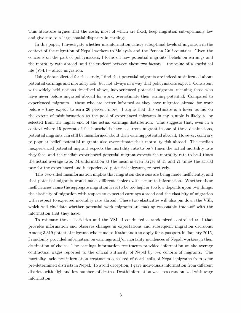
1 Introduction

The number of workers moving across international borders for work is increasing. By 2013, inter-national migrants accounted for over 12 percent of the total population in the global North, over sixtimes the share in 1990 (UNDESA, 2013). The 2011 Gallup poll estimates that more than 1 billionpeople want to migrate abroad for temporary work (Esipova, Ray, and Publiese, 2011). Anecdotesand media reports abound on the risks these migrants are undertaking in search of a better lifefor themselves or their families. For example, more than 3,770 migrants died in the MediterraneanSea in 2015 on their way to Europe (International Organization for Migration, 2015). In 2014,about 445 people died while trying to cross the US-Mexico border (Carroll, 2015). A high deathtoll is not the plight only of those who try to migrate illegally or who are forced to move. TheGuardian reports that almost 1,000 workers, all of whom were legal migrants from Nepal, Indiaand Bangladesh, died in Qatar in 2012 and 2013 (Gibson, 2014).

The intense desire to migrate despite the risks has led policymakers to be concerned thatpotential migrants may have unrealistic expectations about migration. In countries like Nepal,where more than 7 percent of adult, working-age males leave the country for work abroad in agiven year, there is great concern that they make the decision recklessly.1

Policymakers and academics often have contradictory views on whether the level of observedmigration is higher or lower than optimal. Policymakers believe that most potential migrants aremisinformed – in particular, that they expect to earn more than they actually do upon migrationand underestimate the risks of working abroad. Many policymakers also believe that potentialmigrants, knowingly or unknowingly, are trading off risks at unreasonably low prices to the extentthat their experience is often termed exploitative.2 Put together, these notions suggest that theobserved rate of migration is higher than is optimal and that accurate information would lower thelevel.

Academic studies, on the other hand, find migration to be profitable and hugely beneficial forthe marginal migrant and his or her family (see Bryan, Chowdhury, and Mobarak, 2014; McKenzie,Stillman, and Gibson, 2010, for a few examples). These studies suggest that the level of migrationis suboptimal and that increased migration would be welfare improving. If anything, potentialmigrants’ beliefs about earnings and risks are pessimistic, which suppresses migration (as brieflysuggested in Bryan, Chowdhury, and Mobarak, 2014). Alternatively, many academic studies assumethat individuals are fully informed and have rational expectations about the conditions at theirdestinations, and attribute low levels of migration to high costs, monetary and otherwise (seeKennan and Walker, 2011; Morten and Oliveira, 2014; Morten, 2013; Shenoy, 2015, for example).

1An extreme example of the opinion of many policymakers is the following quote from an expert on Nepalimigration: “They go without asking questions. They are not ready to listen. They just want to go. They never evenbother to ask how much they will earn.” (Pattisson, 2013a). Though this statement may be an exaggeration, theview that potential migrants lack information or are misinformed is widely held.

2Migrants working at high-risk jobs for low wages has been dubbed a form of modern-day slavery. Severalnewspaper articles and commissioned research reports express this view (see Deen, 2013; The Asia Foundation, 2013,and other news articles quoted elsewhere in the paper).

2

This literature argues that the costs, most of which are fixed, keep migration sub-optimally lowand give rise to a large spatial disparity in earnings.

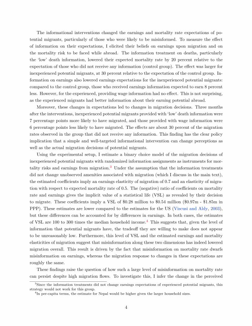
In this paper, I investigate whether misinformation causes suboptimal levels of migration in thecontext of the migration of Nepali workers to Malaysia and the Persian Gulf countries. Given theconcerns on the part of policymakers, I focus on how potential migrants’ beliefs on earnings andthe mortality rate abroad, and the tradeoff between these two factors – the value of a statisticallife (VSL) – affect migration.

Using data collected for this study, I find that potential migrants are indeed misinformed aboutpotential earnings and mortality risk, but not always in a way that policymakers expect. Consistentwith widely held notions described above, inexperienced potential migrants, meaning those whohave never before migrated abroad for work, overestimate their earning potential. Compared toexperienced migrants – those who are better informed as they have migrated abroad for workbefore – they expect to earn 26 percent more. I argue that this estimate is a lower bound onthe extent of misinformation as the pool of experienced migrants in my sample is likely to beselected from the higher end of the actual earnings distribution. This suggests that, even in acontext where 15 percent of the households have a current migrant in one of these destinations,potential migrants can still be misinformed about their earning potential abroad. However, contraryto popular belief, potential migrants also overestimate their mortality risk abroad. The medianinexperienced potential migrant expects the mortality rate to be 7 times the actual mortality ratethey face, and the median experienced potential migrant expects the mortality rate to be 4 timesthe actual average rate. Misinformation at the mean is even larger at 13 and 21 times the actualrate for the experienced and inexperienced potential migrants, respectively.

This two-sided misinformation implies that migration decisions are being made inefficiently, andthat potential migrants would make different choices with accurate information. Whether theseinefficiencies cause the aggregate migration level to be too high or too low depends upon two things:the elasticity of migration with respect to expected earnings abroad and the elasticity of migrationwith respect to expected mortality rate abroad. These two elasticities will also pin down the VSL,which will elucidate whether potential work migrants are making reasonable trade-off with theinformation that they have.

To estimate these elasticities and the VSL, I conducted a randomized controlled trial thatprovides information and observes changes in expectations and subsequent migration decisions.Among 3,319 potential migrants who came to Kathmandu to apply for a passport in January 2015,I randomly provided information on earnings and/or mortality incidences of Nepali workers in theirdestination of choice. The earnings information treatments provided information on the averagecontractual wages reported to the official authority of Nepal by two cohorts of migrants. Themortality incidence information treatments consisted of death tolls of Nepali migrants from somepre-determined districts in Nepal. To avoid deception, I gave individuals information from differentdistricts with high and low numbers of deaths. Death information was cross-randomized with wageinformation.

3

The informational interventions changed the earnings and mortality rate expectations of po-tential migrants, particularly of those who were likely to be misinformed. To measure the effectof information on their expectations, I elicited their beliefs on earnings upon migration and onthe mortality risk to be faced while abroad. The information treatment on deaths, particularlythe ‘low’ death information, lowered their expected mortality rate by 20 percent relative to theexpectation of those who did not receive any information (control group). The effect was larger forinexperienced potential migrants, at 30 percent relative to the expectation of the control group. In-formation on earnings also lowered earnings expectations for the inexperienced potential migrants:compared to the control group, those who received earnings information expected to earn 8 percentless. However, for the experienced, providing wage information had no effect. This is not surprising,as the experienced migrants had better information about their earning potential abroad.

Moreover, these changes in expectations led to changes in migration decisions. Three monthsafter the interventions, inexperienced potential migrants provided with ‘low’ death information were7 percentage points more likely to have migrated, and those provided with wage information were6 percentage points less likely to have migrated. The effects are about 30 percent of the migrationrates observed in the group that did not receive any information. This finding has the clear policyimplication that a simple and well-targeted informational intervention can change perceptions aswell as the actual migration decisions of potential migrants.

Using the experimental setup, I estimate a binary choice model of the migration decisions ofinexperienced potential migrants with randomized information assignments as instruments for mor-tality risks and earnings from migration.3 Under the assumption that the information treatmentsdid not change unobserved amenities associated with migration (which I discuss in the main text),the estimated coefficients imply an earnings elasticity of migration of 0.7 and an elasticity of migra-tion with respect to expected mortality rate of 0.5. The (negative) ratio of coefficients on mortalityrate and earnings gives the implicit value of a statistical life (VSL) as revealed by their decisionto migrate. These coefficients imply a VSL of $0.28 million to $0.54 million ($0.97m - $1.85m inPPP). These estimates are lower compared to the estimates for the US (Viscusi and Aldy, 2003),but these differences can be accounted for by differences in earnings. In both cases, the estimatesof VSL are 100 to 300 times the median household income.4 This suggests that, given the level ofinformation that potential migrants have, the tradeoff they are willing to make does not appearto be unreasonably low. Furthermore, this level of VSL and the estimated earnings and mortalityelasticities of migration suggest that misinformation along these two dimensions has indeed loweredmigration overall. This result is driven by the fact that misinformation on mortality rate dwarfsmisinformation on earnings, whereas the migration response to changes in these expectations areroughly the same.

These findings raise the question of how such a large level of misinformation on mortality ratecan persist despite high migration flows. To investigate this, I infer the change in the perceived

3Since the information treatments did not change earnings expectations of experienced potential migrants, thisstrategy would not work for this group.

4In per-capita terms, the estimate for Nepal would be higher given the larger household sizes.

4

mortality rate for potential migrants following an actual death of a migrant. I take the migrationresponse to an actual migrant death from my other work (Shrestha, 2015), and use the estimatedearnings elasticity and the VSL to translate the migration response into an induced change in beliefson mortality rate. This exercise suggests that potential migrants update their beliefs on mortalityrate by a considerable amount following death events. Additionally, the response is greater whenthere have been more migrant deaths in the recent past. As explored in Shrestha (2015), thesepatterns are inconsistent with models of rational learning. Models of learnings fallacy, such asthe law of ‘small’ numbers, combined with some heuristic decision rules may explain the observedhigh levels of overestimation as well as the sensitivity to recent information about migrant deaths(see Rabin, 2002; Tversky and Kahneman, 1971, 1973; Kahneman and Tversky, 1974, for relatedliterature). Therefore, a fallacious belief-formation process, which leads to high overestimation ofmortality rate abroad among potential migrants, has kept migration levels lower than optimal inthis context.

Apart from providing an important insight into how beliefs can affect migration, this papermakes a methodological contribution to the literature estimating the VSL from revealed preferences.Thus far, much of the empirical literature has taken the route of estimating the wage hedonicregression (see Thaler and Rosen (1976) for a theoretical foundation, and Viscusi and Aldy, 2003and Cropper, Hammitt, and Robinson, 2011 for reviews). One key issue with this literature is that inmany settings, mortality risks are correlated with unobserved determinants of wages confoundingidentification (see Ashenfelter, 2006; Ashenfelter and Greenstone, 2004a, for critiques). In thisstudy, the use of randomized treatments as instruments effectively solves the omitted variablesand endogeneity problem. Further, by directly measuring individual perceptions on earnings andmortality risk, I overcome the bias resulting from measurement error of the risks or the issueof decision-makers being unaware of the true risks (see Black and Kniesner, 2003, for effects ofbiases from measurement errors).5 To the best of my knowledge, this is the first study to estimatethe VSL using exogenous variations in perceived risks and rewards generated from a randomizedexperiment.6

This paper also contributes to the relatively scant literature seeking to quantify the extent ofmisinformation on earnings in context of international migration. McKenzie, Gibson, and Stillman(2013) and Seshan and Zubrickas (2015) find that those who do not migrate, including familymembers, have different expectations about earnings abroad. However, contrary to the currentstudy, these studies find that potential migrants and their family members underestimate thepotential earnings from migration. In a context similar to these studies, Beam (2015) finds that

5Though I elicit subjective perceptions on earnings and wages, it is different from the strand of literature thatestimates VSL by eliciting subjective willingness to pay directly. See Cropper, Hammitt, and Robinson (2011) for areview of this literature.

6This paper is closest in approach to Greenstone, Ryan, and Yankovich (2014) and León and Miguel (2013) who usea discrete-choice framework to study re-enlistment decisions of US soldiers and transportation choices of travelers tothe Sierra Leone airport, respectively. While the institutional settings in their respective contexts drive identificationin these studies, the identification of this study comes from the randomized assignment of information treatments.See Section 6 for a detailed discussion.

5

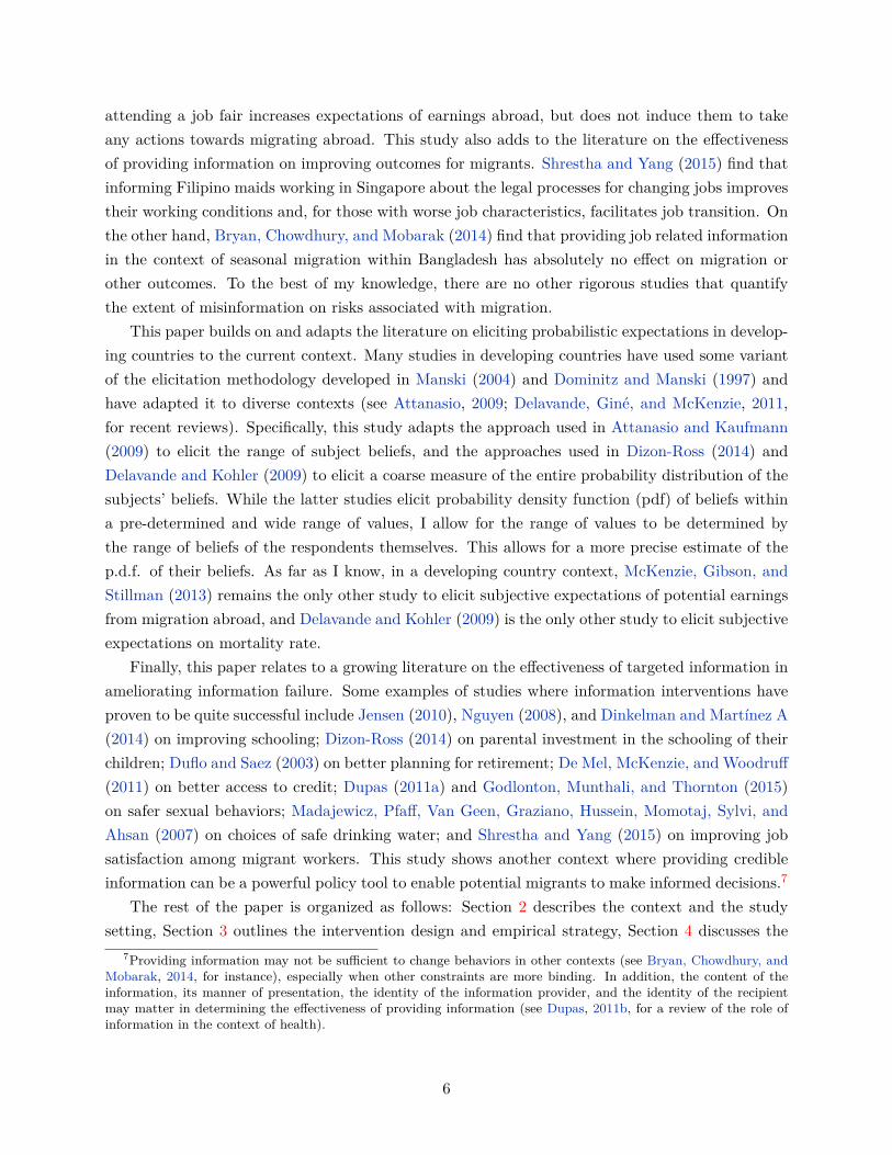
attending a job fair increases expectations of earnings abroad, but does not induce them to takeany actions towards migrating abroad. This study also adds to the literature on the effectivenessof providing information on improving outcomes for migrants. Shrestha and Yang (2015) find thatinforming Filipino maids working in Singapore about the legal processes for changing jobs improvestheir working conditions and, for those with worse job characteristics, facilitates job transition. Onthe other hand, Bryan, Chowdhury, and Mobarak (2014) find that providing job related informationin the context of seasonal migration within Bangladesh has absolutely no effect on migration orother outcomes. To the best of my knowledge, there are no other rigorous studies that quantifythe extent of misinformation on risks associated with migration.

This paper builds on and adapts the literature on eliciting probabilistic expectations in develop-ing countries to the current context. Many studies in developing countries have used some variantof the elicitation methodology developed in Manski (2004) and Dominitz and Manski (1997) andhave adapted it to diverse contexts (see Attanasio, 2009; Delavande, Giné, and McKenzie, 2011,for recent reviews). Specifically, this study adapts the approach used in Attanasio and Kaufmann(2009) to elicit the range of subject beliefs, and the approaches used in Dizon-Ross (2014) andDelavande and Kohler (2009) to elicit a coarse measure of the entire probability distribution of thesubjects’ beliefs. While the latter studies elicit probability density function (pdf) of beliefs withina pre-determined and wide range of values, I allow for the range of values to be determined bythe range of beliefs of the respondents themselves. This allows for a more precise estimate of thep.d.f. of their beliefs. As far as I know, in a developing country context, McKenzie, Gibson, andStillman (2013) remains the only other study to elicit subjective expectations of potential earningsfrom migration abroad, and Delavande and Kohler (2009) is the only other study to elicit subjectiveexpectations on mortality rate.

Finally, this paper relates to a growing literature on the effectiveness of targeted information inameliorating information failure. Some examples of studies where information interventions haveproven to be quite successful include Jensen (2010), Nguyen (2008), and Dinkelman and Martínez A(2014) on improving schooling; Dizon-Ross (2014) on parental investment in the schooling of theirchildren; Duflo and Saez (2003) on better planning for retirement; De Mel, McKenzie, and Woodruff(2011) on better access to credit; Dupas (2011a) and Godlonton, Munthali, and Thornton (2015)on safer sexual behaviors; Madajewicz, Pfaff, Van Geen, Graziano, Hussein, Momotaj, Sylvi, andAhsan (2007) on choices of safe drinking water; and Shrestha and Yang (2015) on improving jobsatisfaction among migrant workers. This study shows another context where providing credibleinformation can be a powerful policy tool to enable potential migrants to make informed decisions.7

The rest of the paper is organized as follows: Section 2 describes the context and the studysetting, Section 3 outlines the intervention design and empirical strategy, Section 4 discusses the

7Providing information may not be sufficient to change behaviors in other contexts (see Bryan, Chowdhury, andMobarak, 2014, for instance), especially when other constraints are more binding. In addition, the content of theinformation, its manner of presentation, the identity of the information provider, and the identity of the recipientmay matter in determining the effectiveness of providing information (see Dupas, 2011b, for a review of the role ofinformation in the context of health).

6

effect of the interventions on perceptions, Section 5 describes the follow-up survey and presents theeffect of the interventions on migration and other outcomes, Section 6 outlines the methodologyfor VSL estimation and presents the results, Section 7 uses the VSL and the elasticity estimates tounderstand the large extent of misinformation on mortality risks, and Section 8 concludes.

2 Context and study setting

With remittances from abroad comprising almost a third of the national GDP, international mi-gration for work is tremendously important for Nepal. In this section, I first describe the nationalcontext of migration to Malaysia and the Persian Gulf countries. I then describe the context specificto this study and compare the study sample with the population of migrants in the country alonga few observable characteristics.

2.1 Context

In recent years, Nepal has been one of the biggest suppliers of low-skill labor to Malaysia andthe Persian Gulf countries. This phenomenon, however, is quite recent. As Appendix Table A.1shows that historically migrant-to-population ratio hovered slightly above 3 percent and was drivenmostly by migration to India, with which Nepal maintains an open border. However, between 2001and 2011, the share of non-India migrants exploded six-fold with only a small change in the shareof India migrants. The rising Maoist conflict in the early 2000s and the economic instability duringthe conflict and in years following the end of that conflict are often cited as key reasons behind thissurge. However, in Shrestha (2014), I find that migration flows to non-India destinations are moreresponsive to shocks in the destination economies than to incomes at the origin. This suggests thatthe booming demand for low-skill labor in Malaysia and the Persian Gulf countries in the 2000s iskey in attracting many Nepali workers.

By 2011, one out of every four households had an international work migrant and almost afifth (18 percent) had a migrant in destinations outside India. More than a fifth (22 percent) ofNepal’s male working-age population (15-45) is abroad, mostly for work. This surge has been drivenby work-related migration to these primary destinations: Malaysia, Qatar, Saudi Arabia, and theUnited Arab Emirates. This type of migration is typically temporary with each episode lasting2-3 years.8 In many of the countries, especially in the Persian Gulf, a work visa is tied to specificemployment with a specific employer.9 It is rare that such migrants eventually end up permanentlyresiding in the destination countries.

The outflow of Nepali workers to these countries has continued to increase in recent years.Appendix Figure A.1 shows the numbers of work permits granted by the Department of ForeignEmployment (DoFE) for Nepali workers seeking employment abroad.10 In 2013 alone, the share

8The modal migration duration to the Persian Gulf countries is 2 years and to Malaysia is 3 years.9Naidu, Nyarko, and Wang (2014) study the impact of relaxing such a constraint in Saudi Arabia.

10The Government of Nepal has allowed private recruitment of workers to certain countries since the mid 90s uponclearance from the Ministry of Labor. The Department of Foreign Employment was established in December 2008 to

7

of males acquiring work permits was about 7 percent of the adult working-age population in thecountry. As a result, remittance income as a share of national GDP increased from a mere 2.4percent in 2001 to about 29 percent in 2013 (The World Bank).

The process of finding jobs in these destination countries is heavily intermediated. Potentialmigrants typically contact (or are contacted by) independent local agents who link them to re-cruitment firms, popularly known as “manpower companies”, in Kathmandu. These local agentsare typically fellow villagers with good contacts in the manpower companies who recruit peoplefor foreign employment from their own or neighboring villages. In addition, most local agents alsohelp potential migrants obtain passports and other related travel documents. The manpower com-panies receive job vacancies from firms (or employment agencies) abroad. They are responsible forscreening (if at all) and matching individuals with job openings, processing contracts, obtainingnecessary clearances from the DoFE, obtaining medical clearances, arranging for travel, visa andother related tasks. Both local agents and the manpower companies receive a commission, whichpotential workers pay prior to departure. It is unclear what fraction of the total costs of interme-diation is borne by the employer, the employee, and what portions of the service charge go to thelocal agents and the manpower companies.11

With a large share of the adult male population working mostly in a handful of destinationcountries, one might expect that information about the risks and rewards of migration would flowback home. Information, especially about earnings abroad, would be expected to flow well amongpotential work migrants though information about mortality rate, due to its rare occurrence, maybe harder to learn. The potential migrants could even use the social network of current migrantsto find work abroad (as in Munshi, 2003).

However, there is a growing sense among policymakers that potential migrants do not haveproper information about the rewards of migration. Anecdotes abound on how migrants discover thetrue nature of their jobs to their frustration and dissatisfaction only upon arrival at their destination.Since the intermediaries are paid only when people migrate, they have financial incentives to distortthe information they provide, drawing potential migrants abroad. Though migrants need contractsfrom employers to receive clearances prior to migration, recruitment agents and agencies commonlyacknowledge that many of these contracts are not honored (the potential migrants may or may notbe aware of this). Further, a large share of the potential migrant earnings comes from over-timecompensation, which may not be explicitly mentioned in the contracts that workers receive. Becauseof these varied and biased sources of information, and because of somewhat fraudulent paperworkpractices, potential migrants are often misinformed about their potential earnings.

Similarly, policymakers and journalists alike are of the opinion that potential migrants aresubmitting themselves to high risk of mortality by migrating to these countries. In recent years,

handle the increased flow of migrant workers to these destinations. The DoFE numbers presented here exclude workmigrants to India and to other developed countries.

11Though the Government of Nepal has agreements with some countries that employers, not potential workers,must pay the cost of migration (including travel costs and intermediation fees), the agreements do not seem to holdin practice. The amounts potential work migrants expect to pay is, in reality, higher than the cost of travel andreasonable levels of intermediation fees.

8

national and international media have given considerable attention to the numbers of Nepali work-ers who die abroad, and to the exploitative conditions they work under. (see Pattisson, 2013b, andseveral ensuing articles in The Guardian, for instance). With a distinctly humanitarian perspec-tive,they portray the system, as a ‘modern-day slavery’. This focus could give potential migrantsa misleading impression of mortality rates, as the stocks of Nepali migrants in these countries arerarely included in these reports. Further, deaths of men of the same age group in Nepal rarelyreceive media or policy attention unless they are a result of some horrific accident. Such biases inreporting could make it much harder for potential migrants to be accurately informed about theunderlying death rates from migration abroad.

All of this culminates in a belief among policymakers that potential migrants, knowingly orunknowingly, are trading high risks at unreasonably low prices. However, policymakers’ beliefs are,after all, beliefs – not often fully guided by rigorous evidence. For instance, there is no evidenceon potential migrants’ actual beliefs on mortality rate and whether they actually respond to mediacoverage of deaths. The higher death tolls could, in fact, simply reflect increased migration to thosedestinations as a result of increased opportunities abroad.

2.2 Study setting and sample

The baseline survey for this study and the experiment was conducted at the Department of Passport(DoP) in Kathmandu in January, 2015. Though Nepali citizens can obtain a new passport fromthe office of the Chief District Officer in their respective district headquarters at a cost of US $50,it takes almost 3 months to receive a passport. On the other hand, if they apply for their passportsat the DoP in Kathmandu, they can opt for the ‘fast-track’ option and obtain their passport withina week at a cost of US $100. Many potential migrants, who are often guided by local agents, usethis expedited service to obtain their passports. DoP officials estimated that during the period ofthe study, an average of 2,500 individuals applied for passports every day. However, not everyonewho has a passport will eventually migrate.12 In fact, many of the study subjects mentioned thatthey were not sure whether they would eventually go for foreign employment and were applyingfor passports just to have the option of going abroad.

For this study, passport applicants who just finished submitting their applications were ap-proached and screened for eligibility for the study. Any male applicant who expressed an intentionof working in Malaysia or the Persian Gulf countries was eligible. Enumerators explained the pur-pose of this study, and those who consented to be interviewed were taken to a designated sectionon the premises of DoP for the full interview.13 At this stage, the passport applicants were toldthat the purpose of the study was to find out how well informed potential migrants were about

12The estimates of the number of Nepali leaving the country hovers around 1,000 to 2,000 per day, many of whommay have old passports.

13Due to the large volume of people submitting their applications, the enumerators could not systematically keepa record of how many people they approached in a day. Though the office accepted applications from 8:00 AM until4:00 PM, most eligible applicants chose the morning hours. On most days, the eligible applicants stopped coming inby 2:00 PM.

9

work migration abroad, and to see how information affected their migration decision. They werenot told the exact nature of the information treatment.

The DoP office is a busy environment, yet the study was conducted in an area reserved exclu-sively for the study, free from outside interference. The DoP restricts non-applicants from enteringthe premises of the office, due to the volume of applicants, so no family members, friends, or localrecruitment agents interfered with the interviews.14 Figure 1 shows the setting, with individualsqueuing at the application counters, and the designated area in the foreground, where enumeratorsare interviewing the respondents and entering their responses in electronic data collection devices.

Between January 4, 2015 and February 3, 2015, we interviewed 3,319 eligible potential migrants.Though the study was conducted in the DoP in Kathmandu, it appears to be representative of thepopulation of current migrants in the country (Appendix Table A.2). The average potential migrantin the study sample is 27.6 years of age and has 7.5 years of schooling, quite similar to the ageand schooling of current migrants in the 2011 census (top panel, columns 1 and 2). It is importantto note that the study sample is predominantly low-skilled. Only 15 percent of the sample hadcompleted more than 10 years of schooling, and only 2 percent had any college education. Thestudy sample is predominantly rural and participants are equally likely to be from the southernplains (Terai) as from the hills and mountains – again, similar to the distribution of migrants inthe census (second panel, columns 1 and 2). Compared to the migrants in the census, the studysample is slightly more likely to be from the mid-western and far-western regions. However, thisdifference could reflect a change in the actual trend as migration has become more ubiquitous in2014 than it was in 2011. Similarly, the distribution of migrants looks similar across Malaysia andthe Gulf countries in both the samples (third panel, columns 1 and 2).

There are three distinct groups of potential migrants in the study sample. There are 1,411“inexperienced” potential migrants who have not yet migrated abroad for foreign employment. Ofthe remainder, 1,341 are “experienced” potential migrants, those who have migrated abroad forwork abroad, but do not have an existing employment contract abroad. That is, these individualshave to search for employment again. The remaining 567 potential migrants are “on leave” fromtheir work abroad. That is, they have an existing employment contract abroad and do not haveto look for work. They are back in Nepal on a holiday and must renew their passports. For theremainder of the paper, I will use this classification unless explicitly noted otherwise.

The average inexperienced potential migrant is younger and slightly more educated than theexperienced one, is 6.4 years younger and has 0.7 more years of schooling (Appendix Table A.2,columns 3 and 4). The difference in schooling is likely to represent the national cohort trend inschooling more than anything else. The geographic distribution of these two groups is quite similar,except that the inexperienced are more likely to be from mid-western and far-western regions thanare the experienced ones – again possibly reflecting a geographic trend as migration became moreubiquitous over the years. In terms of destination choices, the inexperienced are more likely to

14The DoP made an exception for this study by letting the enumerators inside the premises and allowing them toconduct the interviews.

10

want to go to Malaysia than the experienced.

3 Survey design and empirical strategy

The first part of this section describes the nature of the information provided, along with theexperimental design. I then describe the process by which expectations on earnings and mortalitywere measured. The second part of this section discusses balance checks, and the third part presentsthe empirical specification.

3.1 Design of the informational intervention

Each of the eligible male subjects who consented to be interviewed was asked questions on basicdemographics, location and previous migration experience. They were also asked to name thedestination country they were most likely to go to. They were given some information relevant totheir chosen destination. The information was provided verbally by the enumerators as well as inthe form of a card that the respondents could keep for the duration of the interview. The precisecontent of the information depended upon a random number generator built into the data-collectiondevices.

There were three types of information that could be provided to the individuals: basic informa-tion, wage information, and death information. When individuals were selected to receive eitherthe wage or the death information, they could get either the ‘high’ variant of the information or the‘low’ variant. I picked two different information treatment arms because there were no pre-existinginformation on the beliefs of potential migrants. Providing two different information treatmentswould ensure that at least one of them would serve as new information to the potential migrants.Since deliberate misinformation was already a concern in this context, I chose not to deceive them.For the wage information, the only source of information available was the wage reports made byprevious cohorts of migrants to the DoFE in their application to receive the permit for employmentabroad. Therefore, two different years were chosen to generate the ‘high’ and the ‘low’ variant ofthe wage information, and the year the information was pertinent to was stated clearly when pro-viding the information. For the death information treatment arms, I provided information on thedeath toll from a reference district. I varied the reference district to generate the ‘high’ and ‘low’variants. Death toll was provided instead of death rates to emulate the kind of information theywould see in reality. Further, providing respondents with numbers prevents them from repeatingthe same rates when they were asked about their mortality beliefs later in the survey.

The following lays out the precise wording and the content of the information treatments:

1. Basic information: This information was provided to everybody. This contained informationon the number of people leaving Nepal for work in the subject’s destination of choice. Forexample:

Every month, XXXX people from Nepal leave for work in DEST

11

2. Wage information: A randomly chosen third of the respondents did not receive any infor-mation on wages. Another third received the ‘high’ variant with information for 2013, netearnings of $5,700, whereas the remainder received the ‘low’ variant with information for2010, net earnings of $3,000, using the exchange rate at the time of the survey. However,simply adjusting the ‘low’ 2010 numbers for the observed exchange rate increase of 30 percentand yearly inflation rate of 10 percent, would bring the estimate quite close to the ‘high’ 2013numbers. As the year of the statistic was clearly mentioned in the information provided tothem, many seemed to have accounted for the changes themselves. Therefore, the manipula-tion within the two groups is not too large. In any case, the exact wording of the informationwas:

In YYYY, migrants to DEST earned NRs. EEEE only in a month

3. Death information: As with the wage information treatment, a randomly chosen third ofthe respondents received no information on deaths, another third received the ‘high’ variantand the remainder received the ‘low’ variant. The information provided was the numberof deaths of Nepali migrants in their chosen destination from some pre-determined district.For the ‘high’ variant, the district was chosen from the top 25th percentile of the mortalitydistribution in the country, whereas for the ‘low’ variant, the district was chosen from thebottom 25th percentile.15 If the national migrant stock in the destination countries wasevenly distributed throughout all the districts, the ‘high’ death information translated to anannual mortality rate of 1.9 per 1000 migrants and the ‘low’ death information translated toa mortality rate of 0.5 per 1000 migrants. The exact wording of the information was:

Last year, NN individuals from DIST, one of Nepal’s 75 districts, diedin DEST

A built-in random number generator determined what wage and death information (if any) wouldbe provided to each of the respondents. The assignment of wage information treatments wasindependent of the assignment of death information treatments. Figure 2 shows two examples ofthe cards shown to respondents. On the left is an example of the card shown to a respondentintending to migrate to Malaysia for work and who is chosen to receive a ‘high’ wage informationand a ‘low’ death information. On the right is an example of the card shown to a respondentintending to migrate to Qatar for work and who is chosen to receive the ‘high’ death informationand no wage information. The full set of information provided is shown in Appendix Table A.3.Table 1 shows the breakdown of the sample by randomization group.

15Only 1.4 percent of the candidates that received any death information were from the same district as the referencedistrict. 6.8 percent were from a neighboring district of the reference district.

12

3.2 Eliciting beliefs on earnings and mortality rate

After the cards were shown to the respondents, they were asked questions designed to elicit theirbeliefs on earnings and mortality upon migration.16 As discussed in the Introduction, the approachand questions derive from the probabilistic expectations elicitation method of Manski (2004) andDominitz and Manski (1997) adapted to eliciting subjective probability with visual aids in develop-ing countries. At first, the respondents were asked to mention a range of possible monthly earningsfrom migration:

If you worked in this job, what is the min/max earnings that you will make in a month?

When enumerators entered the range in their data-collection devices, the software uniformly dividedthe range into five categories. Enumerators then asked a more detailed question to elicit the entireprobability distribution of their beliefs across the five categories spanning the range of their expectedearnings. The script for the question to elicit the probability density function was:

Now I will give you 10 tokens to allocate to the 5 categories in the range that youmentioned. You should allocate more tokens to categories that you think are morelikely and fewer tokens to categories that you think are less likely. That is, if you thinkthat a particular category is extremely unlikely, you should put zero tokens. Similarly,if you think that a particular category is certain, you should put all the tokens in thatcategory. If you think all of the categories are equally likely, you should put equalnumber of tokens in all of them. There are no right and wrong answers here, so youshould place tokens according to your expectation about your earnings abroad. Notethat each token represents a 1 in 10 chance of that category being likely.

This process of using tokens is similar to that of using beans by Delavande and Kohler (2009) toelicit subjective probability distribution on mortality.

To elicit the range of their beliefs on mortality rates abroad, the following leading question wasasked:

Suppose that 1000 people just like you went to [DEST] for foreign employment for 2years. Remember that these individuals are of the same age, health status, education,work experience and have all other characteristics as you do. Suppose all of them work inthe same job. Now think about the working conditions and various risks they would faceduring their foreign employment. Many people will be fine but some get unlucky andget into accidents, get sick or even die. You may have heard about such deaths yourself.Taking all this into account, of the 1000 people that migrate for foreign employment,at least (most) how many will die within 2 years upon migrating to [DEST]?

16During the pilot, I tried a variant of the questionnaire that elicited expectations both before and after theinformation intervention. The elicitation of expectations constituted the bulk of the questionnaire, and thereforerespondents resorted to anchoring their answers when the same question was asked after the information intervention.Hence, I decided to elicit expectation only once in the survey after the information intervention. Consequently, Icompare expectations across people of different groups.

13

The data-collection devices again automatically divided the range uniformly into five categoriesbased on the range of expected mortality.17 Enumerators then asked the subjects to distribute theten tokens across the five categories based on their beliefs, using a script very similar to the onedescribed above. Enumerators were trained extensively on the scripts and were instructed to bepatient with the respondents. They were instructed to repeat the script as well as give additionalexplanations if the respondents seemed unclear on what was being asked.

To minimize any confusion among respondents, a few confirmatory follow-up questions wereadded to ensure that the question captured their true beliefs. For instance, if someone answered“50” to the first question, a follow-up question would confirm whether they mean 1 out of 20individuals would die. If, in response to the follow-up question, the respondent felt that his initialanswer was not in line with his beliefs, he would reconcile his estimate.

3.3 Balance

Individuals in the initial survey were randomly assigned to various treatment groups based on arandom number generator built into the software of the data-collection devices. Based on therandom number, an appropriate intervention message would appear on the screens, which theenumerators would read out to the subjects after giving them the corresponding information cards.A few characteristics of the respondents were collected prior to randomization: their age, years ofschooling, prior migration experience, location and their intended destination. I check for balance bycomparing means for each of these characteristics between any two arms of each type of intervention.For the death interventions, I compare average characteristics in the control group with the ‘high’treatment group, the control group with the ‘low’ treatment group and finally the ‘high’ treatmentgroup with the ‘low’ treatment group. Appendix Tables A.4- A.9 show the detailed comparisons.

The overall sample looks well balanced with only 2 out of 48 comparisons significantly differentfor death groups at 95 and 90 percent significance levels. Similarly, 3 out of 48 comparisons inthe wage groups are significant at the 95 percent significance level and 4 at the 90 percent level.These results are what one would expect purely from random chance. The joint tests across allcomparisons have a p-value of 0.65 for comparisons within death information treatment arms and0.48 for comparisons within wage information treatment arms, which affirms that randomizationwas balanced across these observable characteristics.

Since most of my analysis focuses on subgroups of inexperienced and experienced migrants, Ipresent balance checks for these subgroups as well.18 For the sample of inexperienced potentialmigrants, only 1 out of 39 comparisons is significantly different at the 5 and 10 percent significancelevels for both types of interventions. This is lower than what one would expect from randomchance. Consequently, for the sample of experienced migrants, of the 42 comparisons, 3 appear

17In cases where respondents gave a range less than 5, they were asked to place tokens in the integer values thatthey mention. For instance, if they mentioned 1 and 4 as their range, they were asked to place token in categories:1, 2, 3, and 4.

18Since the survey did not have a pre-existing pool of potential candidates, randomization was done in-field in realtime without the possibility of a stratification by prior experience.

14

significant at the 95 percent significance level and 7 at the 90 percent level. This is slightly higherthan what one would expect by random chance alone (2 and 4 at the 95 and 90 percent significancelevels). However, the joint test across all outcomes fails to reject equality across the treatmentarms at conventional levels. Furthermore, in all of the empirical specifications to follow, the pointestimates are similar and the substantive results the same with the inclusion or exclusion of thesevariables as controls.

3.4 Empirical specification

The randomized nature of the intervention implies that the basic empirical specification to estimatethe effect of the programs is quite straightforward. I estimate

yi =δ1DeathLoi + δ2DeathHii + α1WageLoi + α2WageHii +Xiβ + εi (1)

where yi is the outcome for individual i, DeathLoi, DeathHii, WageLoi and WageHii are indica-tors of whether individual i receives any of these treatments. Xi are a set of controls which includesfull set of interactions between education categories, age categories and location, indicators for thechosen destination, and enumerator fixed effects. εi represents the error term, and I allow arbitrarycorrelation across individuals at the date of initial survey × enumerators level. The standard errorsremain quantitatively similar with alternative clustering specifications.

4 Does providing information affect perceptions?

Using data from the control group (which does not receive any information on wages or deaths), thefirst part of this section establishes that potential migrants are indeed misinformed about earningsand mortality risks of migration. To do so, I only use the data on the subjects that did not receiveany informational intervention. In the second part of this section, I estimate the impact of theinformational treatment on perceptions about mortality and earnings.

4.1 Descriptive evidence on the extent of misinformation

Misinformation in expected earnings

Misinformation about earnings abroad may persist even in cases where a large share of the popula-tion is a migrant. As discussed earlier, local agents and recruitment companies have an incentive toexaggerate earnings information to induce potential migrants to go. Moreover, previous migrantsmay also provide biased information. They may lie about their earnings to their social networkif they fear social taxation, or feel pressure to maintain any social prestige they gain from havingmigrated abroad (as in McKenzie, Gibson, and Stillman, 2013, Seshan and Zubrickas, 2015, andSayad, Macey, and Bourdieu, 2004). This has fueled concern among policymakers that potentialmigrants may overestimate their earning potential abroad.

15

However, systematic evidence on the degree of such misinformation is rare. To date, there are nocredible surveys of migrants in the destination countries to determine the actual earnings of Nepalimigrants.19 Further, the government does not have a way to track actual earnings abroad. TheDepartment of Foreign Employment only receives reports of contractual earnings from potentialmigrants when they apply for permits to work abroad, and even this data is not publicly available.In this section, I use the survey data I collected to compare potential migrants’ expectations witha few benchmarks to establish that potential migrants are misinformed on their earning potential.

An inexperienced potential migrant expects to earn more than the experienced ones (those whohave migrated before).20 On average, an inexperienced potential migrant expects to earn $12,300(net) from one migration episode, which is 26 percent more than the expectation of those who havemigrated before (Figure 3). This pattern holds for most of the distributions of earnings expectations.Above the 20th percentile, each quantile of expected earnings of inexperienced potential migrantsis higher than the corresponding quantile for those who have migrated before. For instance, themedian inexperienced potential migrant expects to earn 23 percent more compared to the medianmigrant with prior migration experience, and the extent of the discrepancy remains about the sameeven at the 95th percentile.

It is quite striking that the inexperienced migrants expect to earn more than those with greaterexperience and arguably better training. However, the sample of experienced migrants in this studyis non-random: it only includes those who want to migrate again. If good experience in migrationmakes them more likely to migrate again (as in Bryan, Chowdhury, and Mobarak, 2014), then theextent of misinformation presented here is likely to be a lower-bound estimate of the actual gapin information. If experienced migrants migrate for lower earnings abroad because their outsideoption of staying home is much worse, then the extent of misinformation here is likely to be an upperbound. In the current context, however, the former channel is more likely to be predominant.21

The expectations of potential migrants are also much higher compared to the information pro-vided to them. As Figure 3 shows, only 15 percent of the inexperienced potential migrants and 10percent of those who have migrated before expect to earn less than the ‘high’ information providedof $5,700. Virtually no one expects to make less than the ‘low’ information provided of $3,000.However, the official figures may not reflect the actual earnings of migrants abroad as it does notinclude over-time pay, which is often a large share of a migrant worker’s compensation abroad.

In any case, these comparisons, though not perfect, are suggestive of large information gapsbetween the earnings expectations of the inexperienced potential migrants and the actual earnings

19The closest to this approach is the Nepal Migration Survey of 2009 conducted by the The World Bank (2011),which asked household members about the earnings of the foreign migrants. It also asked the returnees the actualearnings they made during their migration episode. Other than the fact that this data was collected almost sixyears ago, it also suffers from reporting biases of the household members, and reflects the misinformation within thehousehold as highlighted in Seshan and Zubrickas (2015).

20Note the change in definition of experienced migrants for this part. For this part, experienced also includes thosewho are back on vacation and have an existing employment contract abroad.

21In the data collected by The World Bank (2011), returnees who earned more are more likely to express a desireto migrate again in the near future. Those who earned above the median during their foreign-migration experienceare 18 percent more likely to express a desire to migrate again.

16

they are likely to accrue once abroad. The actual extent of misinformation for inexperiencedpotential work migrants is likely to be bigger than 26 percent but smaller than that suggested bythe comparison with the official figure.

Misinformation on expected mortality rate

Contrary to the popular notion, potential migrants seem to overestimate their mortality rate abroadby a large factor. The average expected two-year mortality rate of inexperienced migrant is 28 per1000, which is 68 percent higher than the expectations of those who have migrated before. Figure4 shows that not just the mean, but every quantile of expected mortality rate of inexperiencedpotential migrants is higher than the corresponding quantile for those who have prior migrationexperience. For instance, the median expected mortality rate for the experienced is 10 per thousand,whereas it is 5.8 for those who have migrated before. However, these expectations are much highercompared to the actual mortality rate faced by the migrants once abroad. The deaths data fromthe Foreign Employment Promotion Board, the authoritative data source for mortality of Nepaliworkers abroad, and migration data from the Census and the Department of Foreign Employmentshow that the two-year mortality rate of Nepali workers in these destination countries is 1.3 perthousand.22 Only 3 percent of inexperienced potential migrants and 11 percent of those who havemigrated before expect the mortality rate to be lower than what it actually is. The overestimationat the mean is 21 times the actual figure for the inexperienced ones and 13 times for those whohave migrated previously. The extent of overestimation is smaller at the median, but still 8 and4 times the actual rate for both inexperienced and experienced (those who have migrated before),respectively.23

The difference between the actual and reported mortality rates raises the question of whetherthe reports are errors in the reporting of their underlying beliefs or a truthful reporting of theirmistaken beliefs. Reporting of the beliefs could be wrong because, despite measures taken duringthe interview process, subjects may not be able to articulate very small probabilities well (thoughthey say the risk is 5 per 1000, it may be the same for them as 5 per 900, for instance). On theother hand, beliefs could be inaccurate because of biases in information sources as discussed aboveor because of the way potential migrants form beliefs. For most of the paper, I treat the reportedbeliefs as a true reporting of their (biased) beliefs, and I return to address this issue in Section 7with evidence which is consistent with this.

22To put this number in perspective, the mortality rate of average Nepali men with the same age distribution as thesample is 4.7 per 1000 for a two-year period. The mortality rate of average US men with the same age distributionas the sample is 2.85 per 1000 for a two-year period. Note that this information on relative risks was not provided tothe potential migrants.

23The finding that (young) adults overestimate their mortality expectation is not uncommon. Delavande andKohler (2009) find that males aged under 40 in rural Malawi have median mortality expectations that are over 6times the true mortality rate with higher bias for younger cohorts. Similarly, Fischhoff, Parker, de Bruin, Downs,Palmgren, Dawes, and Manski (2000) find that adolescents aged 15-16 in the US overestimate their mortality rate bya factor of 33 even after excluding the “50 percent” responses.

17

4.2 Impact of information on beliefs

To guide the empirical analysis of the impact of information treatments on respondents’ beliefs,Appendix B outlines a simple learning model. In this model, individuals have normally distributedpriors and believe that the information I provided is a random draw from another normal distri-bution. Individuals use Bayes’ rule to form their posterior beliefs, which results in a few testablepredictions about the effect of informational interventions. First, individuals update in the direc-tion of the information. To the extent that potential migrants (especially the inexperienced ones)overestimate their mortality risks and earning potential, information, when effective, would lowertheir perceived mortality risks and earning potential. Second, information lowers the individualvariance of posterior belief, and third, the effect of the information is increasing with the quantileof individual belief distribution. In the rest of this section, I discuss the effect of information onthe beliefs about earnings and mortality risk in light of this framework.

Effect on perception of mortality risks

Consistent with the framework, Table 2 shows that the ‘low’ death information lowers potentialmigrants’ perceived mortality risk of migration by 4 per thousand which is 20 percent of the controlgroup mean (column 1). The effect with the controls (column 2) is only slightly larger. Other infor-mation treatments do not seem to alter the perceived mortality rate of migration by a substantiveamount. For inexperienced potential migrants, providing the ‘low’ death information lowers theirperceived mortality risk of migration by 7.4 per thousand, which is 27 percent of the control groupmean (column 3). Adding controls (column 4) slightly increases this point estimate. The ‘high’death information lowers expected mortality rate by 1.8 per thousand (3.9 with control), but theeffect is not very precise (columns 3 and 4). These effects are consistent with the learning frame-work described in Appendix B and the fact that potential migrants, especially the inexperienced,overestimate their expected mortality rate relative to the truth as well as relative to the informationprovided to them.24 In terms of its effectiveness in filling the knowledge gap, the ‘low’ death infor-mation reduces perceived misinformation by 50 percent, and the ‘high’ death information reducesthe perceived misinformation by 15 percent.25

Furthermore, the ‘low’ death information treatment also lowers the perceived mortality risk ofthe experienced by 2.2 per thousand (3 with controls), which are 13 percent (17 with controls),but are estimated imprecisely (columns 5 and 6). Even though the effect is insignificant, it is quite

24I also find that the inexperienced potential migrants update more drastically when the reference district happensto be their own or a neighboring one, suggesting that potential migrants consider signals from their own or neighboringdistricts as more precise. In fact, among those provided ‘low’ death information from a reference district that happensto be their own or a neighboring district, the average expected mortality rate for those is only 15 per 1000, almosthalf of the control group mean. But since there are only 30 individuals in this group, I do not conduct further analysisusing this variation.

25I define reduction in perceived misinformation as δ

θ0−s , where δ is the effect of the intervention, θ0 is the priormean estimated from the control group, which receives no information, and s is the perceived mean of the signaldistribution as calculated in Appendix B. If s is taken to be the actual value of the information provided to them,the extent of reduction in misinformation is 28 and 8 percent for the ‘low’ and ‘high’ death information, respectively.

18

large and reduces misinformation by almost a third.26 The ‘high’ death information treatment hasan imprecisely estimated positive effect on expected mortality rate for this group. In terms of thelearning framework, this would mean the signal was interpreted as being noisy. Furthermore, theprior of the experienced group is much higher compared to the inexperienced group, which explainswhy the effect of information is opposite for this group.

As I have the entire probability distribution about beliefs of mortality risks, I show the resultson various quantiles of an individual’s belief about the mortality risks in Appendix Table A.10.Consistent with the framework in Appendix B, the result suggests that the information affectedthe entire distribution of the individual belief with larger effects in higher quantiles of their beliefdistribution. For the inexperienced, the ‘low’ death information lowered the average of the 10thpercentile of their beliefs by 6.5 deaths per thousand, which translates to 27 percent of the controlgroup mean. Similarly, the information treatment lowered the average of the 90th percentile oftheir belief by 8.4.

Furthermore, for the inexperienced group, the effect of the information treatment seem to becoming from higher end of the distribution of expected mortality rate. As Appendix Figure A.2shows, the effect of the ‘low’ death information is higher at higher deciles of the expected mortalityrate distribution (bottom right plot). As the figure shows, other information treatments do nothave statistically significant effects at any point of the distribution, except that the effect at thelargest deciles are estimated more imprecisely than others. This suggests that the ‘low’ deathinformation corrects expectations on mortality rates and does so from the individuals who aremore likely to have much higher expectations about mortality rate, and are therefore, more likelyto be misinformed.

These effects suggest that for the inexperienced potential migrants, the ‘low’ death informationtreatment lowered their entire distribution of beliefs on mortality rates consistent with simpleBayesian model of learning described in Appendix B. Further, it lowered the expected mortalityrate from those who would have otherwise had higher expected mortality rates. Consequently, thegroup receiving this treatment had lower variance of the expected mortality rate than the controlgroup.27

Effect on perceptions of earnings

Consistent with the framework, Table 3 shows that the information interventions reduced theexpected net earnings for the inexperienced potential migrants.28 The ‘high’ wage information

26If s is taken to be the actual value of the information provided, then the reduction in misinformation is 14 percent.27I can reject equality of variance between the ‘low’ death information group and the control group using the robust

Levene (1961) as well as Brown and Forsythe (1974) tests. I cannot reject equality of variance in expected mortalityrate for any other pairwise comparison.

28The net earnings from migration is their expected monthly earnings multiplied by the modal duration of a migra-tion episode to their chosen destination after subtracting the expected fees of migrating abroad to that destination.All the effects of the interventions are concentrated in expected monthly earnings with no effect in expected fees(monetary costs) to migrate. The results are almost identical if the analysis is repeated on the (gross) earnings frommigration. I use net earnings simply for ease of interpretation.

19

reduced the expected net earnings by $1,100, which is 8 percent of the control group mean (column3). The ‘low’ wage information reduced expected earnings by $860, only slightly smaller thanthe effect of the ‘high’ wage information treatment. As discussed in Section 3.1, the informationtreatments differed in terms of the year of the statistic, but were similar after the numbers wereadjusted for the inflation and the increase in exchange rate of the destination countries. Therefore,it is not surprising that the effects of these information treatments are also quite similar. In fact,this suggests that inexperienced potential migrants are quite sophisticated in the way they treatthe wage information treatment.

The calculations in Appendix B provides some support for the inexperienced potential migrantsinterpreting the ‘high’ and the ‘low’ wage information in a similar way. Imposing a Bayesian learningmodel on the average inexperienced potential migrant’s beliefs in the control and treatment groups,one can infer the signal mean and variance without using information on the provided signal. The‘high’ wage information was inferred as a signal drawn from a distribution with mean $6,700 andstandard deviation of $1,200. Similarly, the ‘low’ wage information was inferred as a signal drawnfrom a distribution with mean $6,200 and a standard deviation of $1,600. The fact that thesetwo distributions are quite similar is suggestive that the inexperienced potential migrants actuallytreated the ‘high’ and the ‘low’ wage information in a similar way.

Neither of the wage information treatments had any effect on the earnings expectation of theexperienced potential migrants (Table 3, columns 5 and 6). The estimated effects are both small andstatistically indistinguishable from zero. The lack of effect for the experienced potential migrantsis expected as they have better source of information about their earnings potential.

Appendix Table A.11 shows the effect of the interventions on various quantiles of the individual’sprobability distribution of their beliefs on earnings. For the inexperienced potential migrants, the‘high’ wage intervention lowers the 10th percentile of their belief on earnings by about $800 (8percent) and the ‘low’ wage intervention lowers it by $600 (6 percent). As predicted by the simplelearning framework, the magnitudes of these effects become larger for higher quantiles of theirbeliefs.

Furthermore, for the inexperienced group, the effect of the information treatment seem to becoming from higher end of the distribution of expected net earnings. As Appendix Figure A.3shows, the ‘high’ wage information appears to have lowered the earnings expectation more fromthe higher end of the expected earnings distribution whereas the ‘low’ wage information treatmentseems to have lowered perceptions throughout the distribution without a higher effect at the higherend of the distribution. This suggests that individuals who did not completely believe the ‘low’ wageinformation provided are likely to have been at the higher end of the expected earnings distribution.Because of the larger effect of the ‘high’ wage information on higher end of the expected earningsdistribution, this group has lower variance than the control group.29 Here too, the ‘high’ wageinformation managed to squeeze the distribution of expected earnings for the treatment group but

29I reject equality of variance using the Levene (1961) and Brown and Forsythe (1974) tests only for the comparisonbetween the control group and the ‘high’ wage information group and not for other pairs.

20

the ‘low’ wage failed to do so.

5 Does information affect migration and other outcomes?

The initial survey in January 2015 collected phone numbers for the respondent, his wife and a familymember (when available). These subjects were contacted again in April 2015 through a telephonesurvey. The primary purpose of the telephone survey was to determine the migration status of theinitial respondent. Upon contact and consent, enumerators administered a short survey, collectinginformation on migration-related details, job search efforts, and debt and asset positions. The firstpart of this section describes the follow-up survey protocols and discusses attrition. The secondpart discusses the effect of information on migration choices and robustness to various definitionsof migration. The last part of this section describes the impact of informational interventions onother outcomes measured during the follow-up survey.

5.1 Follow-up survey and attrition

Follow-up survey and protocol

These April 2015 follow-up telephone surveys were conducted from the data collection firm’s officeunder close supervision of two supervisors. Enumerators were given specific SIM cards to be usedduring the office hours for the purposes of the follow-up survey. A protocol was developed to reachout to as many initial respondents (or their family members) as possible. Enumerators wouldfirst call the initial respondent’s phone number followed by the wife’s and the family member’sphone number if the former could not be contacted. If anyone picked up the phone, enumeratorsconfirmed the identity of the initial respondent or their family members and made sure that theywere talking about the correct initial respondent. Then enumerators noted the migration statusof the initial respondent: if he was available, they administered the follow-up survey to him; if hehad already migrated, they administered it to the telephone respondent (usually the wife, siblingsor parents). In case the initial respondent was known to be in the country, enumerators madeup to three attempts to administer the follow-up survey to him, before resorting to the telephonerespondent.

If no one could be contacted on any of the phone numbers, then the enumerators would trythe set of phone numbers again at another time or day. Enumerators attempted to call eachset of numbers for six days with at least one attempt every day before giving up on contactingthe subjects. If the telephone respondents were busy at the time of the call, enumerators made anappointment with them and contacted them at a time of their choosing. This protocol was designedto ensure that the subjects, or their family members, were contacted whenever possible and thefailure to contact them either meant that the telephone numbers provided were either wrong orthat the subjects had already migrated.

21

Attrition

Following this protocol, the enumerators were able to conduct detailed follow-up survey with 2,799initial respondents (or their family members) between March 26 and April 24, 2015.30 This rep-resents 84 percent of the overall sample, 85 percent of the inexperienced potential migrants, 86percent of the experienced potential migrants, and only 78 percent for those who had an existingcontract abroad and were back only on a leave. Since the main outcome of interest of the studyis migration, attrition from the survey is also potentially an outcome to the extent that I am lesslikely to obtain information about a migrant.

I consider three separate measures of attrition. The first, Attrition-F, considers whether the fullfollow-up survey was conducted or not. The second, Attrition-M, considers whether it was possibleto determine the migration status of the initial respondent. This measure differs from the firstmeasure when enumerators were able to determine the migration status of the individuals but werenot able to conduct the full follow-up interview. The attrition rate, according to this measure, is13 percent for the overall sample, 12 percent each for the samples of inexperienced and experiencedpotential migrants. Among the 13 percent of the subjects with unknown migration status, it ispossible to know about the attempted calls to the numbers provided by them. The phones of manyin this group were switched off or not in operation, but for a few, the numbers provided were wrong(confirmed either by the telephone operator or by the person who answered the phone). In veryfew cases, the respondents refused to identify themselves or provide any information on the studysubjects. Hence, my third measure of attrition (Attrition-W) indicates confirmed wrong numbersor refusal to interview. According to this measure, the attrition rate is about 3 percent in theoverall sample as well as the subgroups.

The first measure of attrition, Attrition-F, is correlated with the information treatments. Asthe top panel of Table 4 shows, this measure of attrition is higher for death information treatments(marginally significant) and lower for wage information treatments (columns 1 and 2). For theinexperienced potential migrants, the ‘high’ wage information reduces this measure of attrition by4 percentage points, significant at 10 percent level (columns 3 and 4). For the experienced potentialmigrants, the ‘low’ death information increases attrition by 6 percentage points (column 5).

The second measure of attrition, Attrition-M, is also correlated with information treatments.As the second panel of Table 4 shows, this measure of attrition matches the correlation patternobserved for Attrition-F. For the overall sample, death information treatments increase attritionwhereas wage information treatment reduce it (columns 1 and 2). For the inexperienced potentialmigrants, in particular, the ‘high’ wage information treatment lowers this measure of attrition by4 percentage points (columns 3 and 4). Whereas, for the experienced potential migrants, the ‘low’death information treatment increases attrition by 6 percentage points (column 5).

The third measure of attrition, Attrition-W, is not correlated with any of the information30Follow-up surveys ended after a 7.8 magnitude earthquake struck Kathmandu on April 25, 2015, one day ahead

of the planned end date. In the last working day (April 24), only 26 interviews (0.9 percent of total successful follow-up interviews) were conducted. When the follow-up interviews were in full swing, about 120 successful follow-upinterviews were conducted in a day.

22

treatments (bottom panel, Table 4). This measure of attrition is low and, more importantly, notcorrelated with the treatment status. Particularly for the inexperienced migrants, even the directionof the effects does not match the pattern observed for other measures of attrition.

Attriters look broadly similar to non-attriters except for a few characteristics. As AppendixTable A.12 shows, attriters, by all three measures, have similar characteristics as non-attriters inexcept for completed years of schooling (first and second panels). For both the subgroups, I cannotreject the joint null that attriters and non-attriters have the same age, geography and locations.However, attriters have lower completed schooling by more than 1 year compared to non-attriters(first panel, row 2). This also makes some intuitive sense as those who have fewer years of schoolingare likely to have fewer cellphones in the family or could be more likely to misreport phone numbers.However, as seen in Table 4, correlation patterns between treatments and attrition measures remainthe same despite adding controls, including schooling. 31

More importantly, attriters, as classified by the first measures, Attrited-F and Attrited-M,had anticipated earlier migration even during the initial survey in January. In the initial survey,respondents were asked to assign 10 tokens to five bins representing their likely time of migration:0-3 months, 4-6 months, 8-9 months, 10-12 months, and 12+ months. Compared to non-attriters,attriters by those first two measures were more likely to indicate certainty of migrating within threemonths or a much quicker expected migration time (third panel, Appendix Table A.12). However,attriters by the third measure, Attrited-W, did not have different expectations than non-attriters.

This suggests that attriters by the first two measure attrited precisely because they have mi-grated. To incorporate, I define my migration outcome based on different assumptions on theattriters. In measures of migration and other outcome that suffer from missing variables problem,I also estimate the Lee (2009) bounds of effects.

Since the two wage information treatments seem to have similar effects on the expected mortalityand earnings as well as attrition, I pool the two treatments into a single wage information treatmentgroup from this point forward. The results remain essentially the same with the more disaggregatedspecification as well.

5.2 Effect on migration

As discussed above, I have various measures of migration status based on various assumptions thatI make about the attriters. For those whose migration status is observed, I treat them as migrantsif they have already left or are confirmed to leave within two weeks of the follow-up survey.32

For my preferred measure of migration (Migrated-P), I assume all attriters are migrants exceptthose subjects who provided wrong phone numbers or refused to provide any information to theenumerators. That is, this measure of migration treats Attrition-W as missing and considers thosewith switched off or unavailable phones as migrants. With this measure, as shown above, missing

31I also estimate selection on observables correction proposed by Fitzgerald, Gottschalk, and Moffitt (1998) toadjust for the fact that attriters are different from non-attriters. The key results are qualitative and quantitativelythe same. All results presented in the paper are without the correction.

32The results are essentially the same if the confirmed departure time is changed to 1 week or 0 week instead of 2.

23

data is uncorrelated with information treatment and hence the estimates of equation 1 are unbiased.Furthermore, those with phones switched off or unavailable during the follow-up had expected tomigrate earlier and are indeed more likely to be actual migrants.

For the inexperienced potential migrants, migration decision is consistent with the change inexpectations about earnings and mortality rate. As Table 5 shows, ‘low’ death information increasedmigration by 7 percentage points whereas the wage information treatments lowered migration by 6percentage points (top panel, columns 3 and 4). These effects are over 20 percent of the migrationrate observed in the control group. The effects are also what one would expect, given the changein expectations that the treatments induced. The ‘low’ death information lowered the expectedmortality rate abroad, making the destinations more appealing and inducing more them to migrate.On the other hand, the wage information treatments lowered the expected earnings abroad, makingdestinations less attractive and inducing fewer of them to migrate.

The effect on expectations also resonate on migration decision of the experienced potentialmigrants. As Table 5 shows, the ‘low’ death information, which lowered expected mortality ratesabroad increased migration by 9 percentage points (top panel, columns 5 and 6). On the otherhand, the wage information treatments, which failed to induce a change in expectations, also failedto induce a migration response.

The effect of information treatments remain qualitatively and quantitatively similar for thesecond measure of migration (Migrated-A). This measure of migration treats all attriters as havingmigrated. As the second panel of Table 5 shows, the effect of information treatments on thismeasure of migration is quite similar to the effect on the preferred measure (Migrated-P).

Because of the missing variables problem, the effect of the information treatments on the ba-sic measure of migration (Migrated-B) is biased. This measure treats all those individuals withunconfirmed migration status (Attrited-M) as missing. For the inexperienced potential migrants,‘low’ death information is not correlated with Attrited-M, and hence, as Table 5 shows, the effecton this measure of migration is almost the same as for the previous two measures of migration(bottom panel, columns 3 and 4). However, the effect of wage information treatment is two thirdsthe size of the effect for other measure of migration. This is precisely what one would expect ifwage interventions led the potential migrants to not migrate and therefore more likely to be foundduring the follow-up survey.

The third panel of Table 5 shows the results for this measure of migration (Migrated-B). Forthe inexperienced potential migrants, ‘low’ death information treatment increased migration by 7percentage points. This effect, significant at 5 percent level, is almost 30 percent of the migra-tion rate in the control group. For this group, death ‘high’ information also increases migrationslightly (9 percent) but the effect is insignificant. Note that since missing data (Attrition-M) isnot correlated with death interventions, these points estimates similar to the preferred measure ofmigration. However, since missing data (Attrition-M) is correlated with wage information treat-ments, the point estimate for wage information treatments is lower and not significantly differentfrom zero at conventional levels. This is precisely what one would expect if wage interventions led

24

the inexperienced potential migrants to not migrate and therefore more likely to be found duringthe follow-up survey. Similarly, for the experienced migrants, ‘low’ death information, which in-creased attrition, has a smaller effect than for other measures. Again, this is what one would expectif ‘low’ death information led the experienced potential migrants to migrate more and therefore lesslikely to be found during the follow-up survey.

Lee (2009) bounds on effect of the information treatments on the basic measure of migration(Migrated-B), also supports that attrition (Attrited-M) captures unobserved migration. As Table6 shows, the bounds on the effects of the death information treatments for inexperienced potentialmigrants are tight and similar in magnitude as the effect on the preferred measure of migration(second panel, columns 1 and 2). However, the lower bound on the effect of wage informationon migration is similar to the effect on the preferred measure (Migrated-P) whereas the upperbound on the effect is similar to the effect on the basic measure (Migrated-B). That is, selectivelydropping a random subset of those who migrated and are from the wage information treatmentgroup, in order to balance attrition, produces an estimate not too different from the effect onthe basic measure (Migrated-B). However, selectively dropping a random subset of those who didnot migrate and are from the wage information treatment group to balance attrition produces anestimate different from the effect on the basic measure and very similar to the effect on the preferredmeasure (Migrated-P). This also suggests that attrition is likely to be more among migrants thannon-migrants.

5.3 Effect on other outcomes

In this section, I investigate the effect of the information treatments in other outcomes that werecollected using the full follow-up survey. This would shed light on other effects of the interventionor the mechanism of the migration effect. Since these measures were collected through the fullfollow-up survey, these measures suffer from attrition (Attrition-F).

Appendix Table A.13 shows that the information treatments did not affect whether the poten-tial migrants choose the same country or region (Persian Gulf versus others) as they did during theinitial survey. Between the initial survey and the follow-up, about 40 percent of the inexperiencedand 28 percent of experienced potential migrants changed their destination country. The informa-tion treatments barely changed this – the effects are not just statistically insignificant, but alsonumerically small. The same holds true for potential migrants changing their intended (or chosen)destination region.

The wage information increases the chance that inexperienced potential migrants seek newmanpower companies, but has no effect on seeking consultations from other source. As AppendixTable A.14 shows, inexperienced migrants receiving wage information are 6 percentage points morelikely to consult different manpower companies after the initial survey (top panel, columns 3 and4). This effect is 26 percent of the likelihood in the control group. The Lee (2009) bounds onthis estimate are positive and large, suggesting that the effect is large despite the missing variablesconcern (Appendix Table A.15, middle panel, column 3). This probably reflects an action that

25

inexperienced potential migrants can take upon realizing that they had been misinformed. However,none of the information treatments affect whether they consult with family members or friends (midand bottom panel, Appendix Table A.14). Similarly, none of the information treatments affectsany of these outcomes for the experienced potential migrants.

As Appendix Table A.16 shows, none of the information treatments changed whether householdstook out new loans (top panel), paid back old loans (mid panel), or bought new assets (bottompanel). However, for the experienced potential migrants, the ‘low’ death information increases theprobability that they bought new assets between the two rounds of the survey and wage informationreduces the likelihood of buying new assets. The wage result is particularly inconsistent with therest of the results as it did not affect perceptions or expectation or any other outcome, hence Iattribute this odd result to random chance.

6 Estimates of VSL

Since the information treatments are effective in changing the expectations of inexperienced poten-tial migrants concerning both earnings and mortality rate associated with migration, I estimate thevalue of a statistical life (VSL) for this group by using the information treatments as instruments.The first part of this section describes the methodology and the contribution of this paper in es-timating VSL, the second presents the estimates for the pool of inexperienced potential migrants,and the third explores robustness. The final part estimates the VSL for various subgroups.

6.1 Methodology and contribution

Schelling (1968) shaped the way economists think about VSL as the willingness to trade-off wealthW for a marginal change in the probability of death d holding everything else constant. That is,

V SL = dW

dd

holding everything else, including utility, constant.The empirical approach to estimating VSL in this context can be motivated by a simple binary

choice framework. The utility that a potential migrant i receives from migrating can be written as

UMi = α+ βdi + γWi + εi

whereWi is the expected earnings from migration, di is the expected mortality risk from migration,and εi represents the unobserved individual specific factors that influence the utility from migration.The utility that the potential migrant i receives from not migrating is unobserved and can simplybe written as UHi = α′ + ui. Then the migration decision Mi of potential migrant i is given by

Mi =1(UMi > UHi

)=1

(ui − εi < α− α′ + βdi + γWi

)26

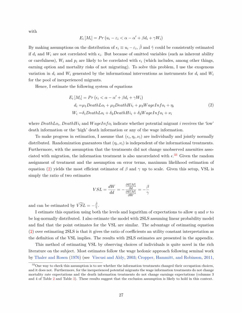
withEi [Mi] = Pr

(ui − εi < α− α′ + βdi + γWi

)By making assumptions on the distribution of εi ≡ ui− εi, β and γ could be consistently estimatedif di and Wi are not correlated with εi. But because of omitted variables (such as inherent abilityor carefulness), Wi and pi are likely to be correlated with εi (which includes, among other things,earning option and mortality risks of not migrating). To solve this problem, I use the exogenousvariation in di and Wi generated by the informational interventions as instruments for di and Wi

for the pool of inexperienced migrants.Hence, I estimate the following system of equations

Ei [Mi] = Pr(εi < α− α′ + βdi + γWi

)di =µ1DeathLoi + µ2DeathHii + µ3WageInfoi + ηi

Wi =δ1DeathLoi + δ2DeathHii + δ3WageInfoi + νi

(2)

where DeathLoi, DeathHii andWageInfoi indicate whether potential migrant i receives the ‘low’death information or the ‘high’ death information or any of the wage information.

To make progress in estimation, I assume that (εi, ηi, νi) are individually and jointly normallydistributed. Randomization guarantees that (ηi, νi) is independent of the informational treatments.Furthermore, with the assumption that the treatments did not change unobserved amenities asso-ciated with migration, the information treatment is also uncorrelated with ε.33 Given the randomassignment of treatment and the assumption on error terms, maximum likelihood estimation ofequation (2) yields the most efficient estimator of β and γ up to scale. Given this setup, VSL issimply the ratio of two estimates

V SL = dW

dd= −

∂E[M ]∂d

∂E[M ]∂W

= −βγ

and can be estimated by V SL = − βγ .

I estimate this equation using both the levels and logarithm of expectations to allow η and ν tobe log-normally distributed. I also estimate the model with 2SLS assuming linear probability modeland find that the point estimates for the VSL are similar. The advantage of estimating equation(2) over estimating 2SLS is that it gives the ratio of coefficients an utility constant interpretation asthe definition of the VSL implies. The results with 2SLS estimates are presented in the appendix.

This method of estimating VSL by observing choices of individuals is quite novel in the richliterature on the subject. Most estimates follow the wage hedonic approach following seminal workby Thaler and Rosen (1976) (see Viscusi and Aldy, 2003; Cropper, Hammitt, and Robinson, 2011,

33One way to check this assumption is to see whether the information treatments changed their occupation choices,and it does not. Furthermore, for the inexperienced potential migrants the wage information treatments do not changemortality rate expectations and the death information treatments do not change earnings expectations (columns 3and 4 of Table 2 and Table 3). These results suggest that the exclusion assumption is likely to hold in this context.

27

for review of empirical estimates). Thaler and Rosen (1976) show that the slope of the observedmarket locus in the wage-mortality risk plane gives the willingness to pay of the workers to avoidmarginal increments in mortality risks (i.e. the VSL). But getting consistent estimate of the marketlocus (or its slope) has been difficult because of two key problems.

First, in most estimations using the wage hedonic approach, mortality risk is correlated withunobserved determinants of wages (see Ashenfelter, 2006, for a critique). This introduces a se-lection bias in the estimates with an unknown direction and magnitude of the bias. The currentstudy overcomes this problem by using exogenous variation in (expected) earnings and (expected)mortality risks generated by randomly provided information.34

The second issue with the wage hedonic approach is that mortality risks are measured witherrors and maybe known imperfectly to agents. Black and Kniesner (2003) emphasize that themeasurement errors are non-classical in nature and leads to large biases in either direction.35 Inthis study, I directly measure expectations on earnings and mortality risks without the need toworry about whether they (as well as the econometrician) know the actual mortality rate and theearnings involved.36 Rather than the actual risks involved with the occupation, it is the perceivedrisks that is actually relevant in the decision-making process.

The second, and somewhat new, approach to estimating VSL is by modeling the choices madeby individuals or populations. In this vein, Ashenfelter and Greenstone (2004b) model the decisionof states to adopt a higher speed limit to compute VSL. In their setting, states choose to adopthigher speed limit if the monetary value of times saved per marginal fatality is higher than the VSL.The authors estimate the monetary value of times saved per marginal fatality by instrumentingfatalities with a plausibly exogenous increase in speed limits in rural interstate roads in the USfrom 55 mph to 65 mph in 1987. Though this gives them a well identified upper bound estimateof the VSL, their estimates of actual VSL suffers from lack of exogenous variation in modeling thedecision of the states to adopt the speed limit. Furthermore, this VSL is the tradeoff by the state(or the median voter if the preference of the states represent the policy choices of the median voter)and could be different from the tradeoff made by individuals.

In a more refined modeling of individual choices, Greenstone, Ryan, and Yankovich (2014) studythe reenlistment decision (and occupation choices within the military) of US soldiers when facedwith varying monetary incentives and mortality risks. In a methodology similar to this paper, theauthors infer the VSL of US soldiers by looking at the ratio of coefficients on mortality risk andmonetary incentives of a discrete choice model of occupation choice. The identifying variation intheir study comes from the institutional process that determines compensation for reenlistment andvariety of occupations undergoing different mortality risks as the US engages in various militaryactions. Another study that employs the discrete choice framework to estimate the VSL is León and

34Lee and Taylor (2014) is one of the rare studies to estimate VSL using an exogenous variation in plant level risk.They exploit the random assignment of federal safety inspection to instrument for plant level risk to estimate theequilibrium relationship between wages and risks.

35In fact, they estimate VSL to be negative in half their specifications.36This, of course, is assuming that the respondents are able to articulate the risks accurately during the survey.

28

Miguel (2013), which examines the transportation choices made by travelers to the internationalairport in Sierra Leone. The identifying variation in this study comes from the availability ofdifferent options at different periods over which the data was collected.

This study is methodologically similar to Greenstone, Ryan, and Yankovich (2014) and Leónand Miguel (2013), as it infers VSL from the ratio of coefficients in a model of migration choicesof potential migrants, but it extends the approach with a randomized information experiment thatintroduces exogenous variation in perceptions of earnings and mortality risks. To the best of myknowledge, this is the first study to employ randomized controlled trial in estimating the VSL.

6.2 Estimates of VSL for inexperienced potential migrants

Both the logarithmic and the levels specifications estimate migration elasticities that are quite sim-ilar across specifications. As Table 7 shows, across all three measures of migration, an increase in(logarithm of) expected mortality rate lowers probability of migration and an increase in (logarithmof) expected earnings increases migration probability as expected (top panel). For the preferredmeasure of migration (Migrated-P), an increase in one percent in expected mortality rate reducesmigration by 0.16 percentage points (column 1). This translates to an elasticity of migration toexpected mortality risk of 0.5. Similarly, an increase in one percent in expected earnings increasesmigration by 0.22 percentage points, which translates to an elasticity of migration to expectedearnings of 0.7. The bottom panel of the table estimates similar elasticities with the levels spec-ification. An increase in expected mortality rate by 1 percentage points reduces migration rateby 6 percentage points (column 1). This point estimate translates to an elasticity of 0.5, which isexactly the same elasticity from the logarithmic specification. An increase in expected earnings by$1000 increases migration rate by 1.1 percentage points which implies an elasticity of 0.5 which isonly slightly smaller compared to the elasticity estimated using the logarithmic specification. Sinceexpected mortality and expected earnings are more likely to follow a log-normal distribution thana normal distribution, I prefer the estimates with logarithms rather than levels.37

These estimates suggest that misinformation has actually lowered the migration rate becausepotential migrants overestimate mortality more than they overestimate earnings. If inexperiencedpotential migrants had true information on the mortality risk (1.3 per 1000 for two-year periodinstead of 27.57), migration would increase by 47 percentage points from its current level (assumingthe effect are the same for large changes in perceptions). Similarly, if inexperienced potentialmigrants had the same net earnings expectations as the experienced ones ($9,660 instead of $12,270),migration would decrease by 5 percentage points. The net effect on migration would therefore bean increase of 42 percentage points – a remarkable 140 percent. Even assuming a much lower actualearnings of $6,000 for the inexperienced (since the expectations of the experienced are likely to bean upper bound on the counterfactual earnings), migration would still go up by by 31 percentagepoints (102 percent from the current level).

37I cannot reject the null of normality for the log of both expectations in the untreated group using a Kolmogorov-Smirnov test. However, the more stringent forms of the test reject normality.

29

The VSL implied by this choice is the ratio of the marginal effect of the expectations on migrationdecision. For the logarithmic specifications, the estimates of VSL range from $0.28 million to $0.63million, depending upon the different measures of migration used (top panel, Table 7). The VSLusing the preferred measure of migration (Migrated-P) is estimated more precisely than others butthe estimated magnitudes are quite similar. For the levels specification, the estimates of the VSLrange from $0.43 million to $2.35 million for various measures of migration (bottom panel). Thelevels specification yields larger and noisier estimates than the logarithmic specifications. Exceptfor the measure of migration with attrition problem (Migrated-B), all the estimates are statisticallydifferent from zero and qualitatively similar to their logarithmic counterparts. The VSL from thepreferred measure with the levels specification is $0.54 million and its logarithmic counterpart iswithin one standard error from this estimate. 38

Comparison with estimates in the literature

It is hard to compare these estimates of VSL, estimated for the pool of potential internationalmigrants from Nepal, to most estimates in the literature, which apply to the US labor market.As reviewed in Viscusi and Aldy (2003) and Cropper, Hammitt, and Robinson (2011), typical USestimates range from $5.5 million to $12.4 million (in 2014 US$).39 The preferred estimates in thisstudy ranges from $0.28 million to $0.54 million ($0.97 million to $1.85 million in PPP$).40 It isreasonable to expect a lower VSL in the context of Nepal compared to the US as the average Nepalipotential migrant has a much lower income: US GDP per capita is 23 times the GDP per capitaof Nepal in PPP terms. In fact, several studies find the developing country estimates of the VSLare in general lower than the estimates from the US (in Viscusi and Aldy, 2003, for example).41

Nevertheless, the VSL estimates in this paper are a comparable proportions of the median householdincome in Nepal as the estimates in the US: 150 to 300 times the median household income in Nepalversus 100 to 250 times that in the US.

Estimates for populations outside the US, especially for developing countries, is quite rate andvary widely. For instance Kremer, Leino, Miguel, and Zwane (2011) estimate the VSL of lessthan $1000 based on the revealed willingness of Kenyan households to travel further for cleanerwater. León and Miguel (2013) estimate a VSL of $0.6m to $0.9m from the revealed choices ontransportation options while traveling to the international airport in Sierra Leone. Greenstoneand Jack (2015) highlight the paucity of VSL estimates in developing countries and call for moreresearch in developing revealed preference measures of the willingness to pay for lower mortality(through improving environment quality).

38The 2-SLS estimation of equation (2) produces very similar point estimates for VSL but are estimated with largerstandard errors (results in Appendix Table A.17).

39Deflated using Urban CPI series.40Using PPP conversion factor (US$ to PPP$ for Nepal) of 3.45 from The World Bank.41Interestingly, the estimates of VSL from Greenstone, Ryan, and Yankovich (2014) ($0.18 million to $0.83 million

in 2014 US$) are more in line with those from this study. However the VSL is expected to be much lower among USsoldiers, who probably have higher preference for risky activities, than the average American. In fact, even withinthe soldiers, the authors find a lower VSL for those taking risky jobs.

30

6.3 Robustness to various points on the belief distribution

If potential migrants have uncertain priors about earnings and mortality rate while abroad, thenthey may not act as expected utility maximizers who maximize the probability weighted average ofutilities in various states of the world. In such cases, the expected value of their beliefs may not bethe right measure that influences their migration decision. It could be possible that people behavein an uncertainty-averse manner and use a different utility maximization rule. For instance, Gilboaand Schmeidler (1989) propose a max-min rule where agents maximize utility assuming the worstpossible state. In this part, I explore robustness of the VSL estimates to using alternative pointsin their belief distribution.

Table 8 shows that the estimates in Section (6.2) are robust to a few alternative decision-makingrules. In column 1, I assume that individuals are extremely cautious about migrating and assumethe worst. That is, they assume that the actual mortality risk is the highest end of their beliefdistribution and the actual earnings, at the lowest. With this assumption, the estimated VSL is$0.16 million using the logarithmic specification and $0.37 million using the levels specification.These estimates are smaller than those in Table 7 but are unlikely to be statistically different.Similarly, column 3 assumes the opposite of column 2: that the individuals take the most optimisticview in making their migration decision. They assume that earnings are the highest end of the beliefdistribution and mortality is the lowest end of their belief distribution. With this assumption, theestimated VSL is slightly higher but statistically similar to the corresponding estimates in Table7. Column 2 performs this exercise assuming that the midpoint of their belief distribution are therelevant parameters and column 5 does the same assuming that their most strongly held beliefs arethe relevant parameters. Both of these exercises produce slightly lower estimates than Table 7, butwell within a margin of statistical errors. This table suggests that the estimates of VSL are quiterobust to alternative decision-making rules on migration with the estimates ranging between $0.16million to $0.32 million with the logarithmic specification and $0.35 million to $0.61 million withthe levels specifications.

6.4 Estimates of VSL for subgroups of inexperienced potential migrants

In this part, I present VSL estimates of equation (2) for various subgroups of the inexperiencedpotential migrants. Table 9 presents results of these estimates.

As Table 9 shows, the older half of the inexperienced potential migrants seem to have higherbut less precisely estimated VSL than the younger ones (columns 1 and 2). The difference is drivenby the differences in elasticities with which migration responds to changes in expectations. Theimplied elasticities of migration with respect to expected mortality and earnings are 0.4 and 0.2respectively for the old whereas they are 0.6 and 1.1 for the young.

Columns (3) and (4) show the results bifurcated by education level. The low group refers tothose with at most 8 years of schooling (below median) and the high group refers to the rest. Eventhe high education group is low-skill with average schooling of 10 years. The low education grouphas an average schooling of 5 years (median of 6 years). The low educated group is quite sensitive

31

to changes in expected mortality (elasticity of 0.6) but extremely insensitive to changes in expectedearnings (elasticity of 0.05). Hence, this group has extremely large but imprecisely estimated VSL.Similarly, the more educated groups are also less sensitive to changes in expected earnings withan elasticity of 0.16. However, the earnings estimates are quite noisy. This subgroup analysisis less informative than the previous one as the responsiveness to changes in expected earningsis estimated with large standard errors. A change in specification (for example, using the levelsinstead of logarithms) or estimating the equation using 2SLS (as in Appendix Table A.19) doesnot improve precision of this estimate. It is possible that the responsiveness to expected earningsdoes not vary much by education (at least in this range of low schooling in the data) and hence,splitting the sample this way leads to nothing but a loss in statistical power.

Inexperienced workers who choose manual work have lower estimated VSL than those whopick non-manual work (column 5 and 6). It is important to note that even the jobs classified asnon-manual are low-skilled, labor-intensive work as drivers, guards, security personnel, domesticworkers, and hotel and restaurant workers. The difference between these two subgroups arises,again, from the difference in responsiveness to changes in expected earnings. The manual laborersare more than twice as responsive as the non-manual workers to changes in expected earnings withan elasticity of 1.0. Hence, this group has a lower VSL of $0.14 million compared to the workers innon-manual group with a (imprecisely estimated) VSL of $0.41 million.

7 Why is expected mortality rate so high?

Section 6.2 establishes that the estimated VSL are reasonable and that misinformation actually hasled to lower migration in this context. At the implied willingness to trade off earnings for mortalityrate, migration is suppressed because of extremely high expectations of mortality rate relative tothe truth. In this section, I show that the high mortality rate expectation is a consequence ofover-inference by potential migrants in response to actual migrant deaths rather than misreportingor an artifact of data collection method.

The instrumental variables estimate of the VSL and the migration elasticities are consistenteven though the expectations are measured with error. The instrumental variables estimate alsosolves any measurement issue that can be modeled as an additive component (either in logarithmicor in levels of the expectations). Hence, I use the VSL and the elasticity estimates, along withmy estimates from Shrestha (2015) to infer the change in perceived mortality rate for potentialmigrants in response to a single migrant death.

In Shrestha (2015), I find that, after controlling for an array of confounding fixed effects, onemigrant death in a district reduces monthly migrant flow from that district by 0.9 percent for 12months. This represents a total of 11 percent reduction of monthly migrant flow (albeit over a year)in response to a single death. I then calculate a one-time increase in migrant earnings necessaryto induce the same number of potential migrants to migrate so that the net effect on migration iszero. Using the earnings elasticity of migration estimate of 0.7 from Section 6.2, I find that migrant

32

earnings need to increase by 15 percent. That is, a one-time increase in migrant earnings of 15percent will offset the reduction in migrant flows caused by a single migrant death.

Finally, I use the estimate of VSL from Section 6.2, to translate the change in earnings tochange in perceived mortality rate. I use the following discretized formulation of the VSL and theelasticities to do so,

∆d = ∆WV SL

= 1V SL

· β · 1ε·W (3)

where d represents the perceived probability of death and W is the average potential earnings frommigration, β is the migration effect of the death, and ε is the earnings elasticity of migration.Using the preferred estimate of VSL and β

ε = 0.15 from above, I find that the change in perceivedprobability following a single death in the district is 6.7 per thousand.42

The high perceived mortality rates expressed by the potential migrants are consistent withthe effect on perceptions generated by a single death and their exposure to migrant deaths. Theinexperienced potential migrants expect the mortality rate to be 27.6 per thousand per migrationepisode. From the estimates above, they only need 4.1 deaths in their district to generate this levelof expected mortality rate starting form a prior of zero. In 2013, an average district experienced 4.3deaths in five months, suggesting that such high level of mortality perception can be generated evenif potential migrants are making decisions about mortality risks only based on past five months ofmigrant mortality incidences in their districts.

In Shrestha (2015), I also find evidence that potential migrants react more adversely when therehave been more migrant deaths in the recent past. Subsequent migrant flow falls more drasticallyin response to a migrant death in districts which have experienced many migrant deaths in therecent past compared to the response in districts which have experienced few migrant deaths inthe recent past. That is, potential migrants seem to be over-weighting recent deaths in formingtheir priors on mortality rate. In Shrestha (2015), I show that the amount of updating following amigrant death, and the responsiveness of updating recent deaths cannot be generated by a rationalBayesian learnings model. A model of a learning fallacy, the law of ‘small’ numbers, correctlypredicts the over-inference result as well as the dependence on the number of deaths in the recentpast (see Rabin, 2002, for mathematical formulation). Belief in the law of ‘small’ numbers, inconjunction with availability or other heuristic decision rule could also explain the high observedoverestimation of mortality rate (as in Tversky and Kahneman, 1971, 1973; Kahneman and Tversky,1974). One such heuristic explanation could be that potential migrants do not pay attention tomigrant deaths unless they are actively thinking about migrating abroad, in which case they formtheir priors by observing migrant deaths in their districts in the past few months. Since they alsocommit the fallacy of believing in the law of ‘small’ numbers which makes them over-infer fromrecent information such as actual migrant deaths in the district or even the information providedin this study.

42Assuming that each component of equation (3) is normally distributed with the estimated mean and variance,and also that these components are uncorrelated with each other, the standard error for the change in perceivedmortality rate is 3.72. The calculation is robust to using VSL and elasticity estimate from the levels specification,which results in a change in perceived mortality rate of 5.8 per thousand.

33

Hence, the high expectation of mortality rate among potential migrants is consistent with theexperience potential migrants probably have and the way they appear to process it. The large extentof misinformation seems to be driven by the fallacious way they form their priors on mortality rateabroad.

8 Conclusion

The gain from international migration is expected to be huge, but there could still be importantnon-institutional barriers to migration. I show that misinformation about both the rewards and riskassociated with migration could be important deterrent, even in a context where a large share ofpopulation migrates for work. I find that potential work migrants from Nepal to Malaysia and thePersian Gulf countries overestimate their earnings potential as well as the mortality rate abroad.Contrary to the prevalent belief among policymakers , the extent of overestimation of mortalityrate far outweighs the extent of overestimation of earnings. Individuals are not migrating recklesslyby trading off high mortality risk for small increase in earnings: the estimated VSL of $0.28 millionto $0.63 million, revealed from their decision to migrate, is quite reasonable for a poor population.Therefore, at their current willingness to trade off mortality risk with earnings, they would be morewilling to migrate abroad if they had accurate information about the earnings and mortality riskabroad.

However, the reason for low migration in this study is distinct from those seen in the literature.Though misinformation on earnings has been documented previously in other contexts, most no-tably in McKenzie, Gibson, and Stillman (2013), misinformation on the risks of migration has not.This finding suggests that information frictions, particularly about risks that workers face abroad,could suppress migration substantially. Failing to take these into account could lead researchersto estimate high (fixed) costs of migration. In this regard, the estimated costs of migration haveto be interpreted not just as monetary and psychic, but also as perceived cost, stemming frommisinformation on earnings and, more importantly, risks.

Furthermore, in conjunction with my findings in Shrestha (2015), I show that such misinforma-tion on mortality rate may arise because of fallacious inference by potential migrants. I find theyseem to drastically update their beliefs about the mortality rate in response to an actual death of amigrant. Furthermore, the response to a migrant death is larger when potential migrants have seenmore migrant deaths in recent months. While models of rational Bayesian learning fail to generatethe magnitude of updating or the dependence on recent migrant deaths, models of learning fallacy,such as the law of ‘small’ numbers, combined with some heuristic decision rules can explain thelarge observed overestimation.

Finally, this paper presents a novel and credible way to estimate the VSL of inexperiencedpotential work migrants from Nepal. I estimate the VSL by exploiting the exogenous variationin expectation of earnings and mortality risks generated by randomly provided information in amodel of migration decision. Two features of this setting make this approach to estimating the

34

trade-off between earnings and mortality rate feasible. First, inexperienced potential migrants aremisinformed about the mortality rate as well as earnings they could make abroad. Second, theyare responsive to information provided to them and their migration choices reflect the changedperceptions induced by the information treatments. This approach could potentially be applied toother settings that meet the two criteria.

35

ReferencesAshenfelter, O. (2006): “Measuring the Value of a Statistical Life: Problems and Prospects,”The Economic Journal, 116(510), C10–C23.

Ashenfelter, O., and M. Greenstone (2004a): “Estimating the value of a statistical life: Theimportance of omitted variables and publication bias,” American Economic Review Papers andProceedings, 94(2), 454–60.

(2004b): “Using mandated speed limits to measure the value of a statistical life,” Journalof Political Economy, 112, pS226–S267.

Attanasio, O., and K. Kaufmann (2009): “Educational choices, subjective expectations, andcredit constraints,” Discussion paper, National Bureau of Economic Research.

Attanasio, O. P. (2009): “Expectations and perceptions in developing countries: Their measure-ment and their use,” The American Economic Review Papers and Proceedings, 99(2), 87–92.

Beam, E. (2015): “Do job fairs matter? Experimental evidence from the Philippines.,” Journal ofDevelopment Economics.

Black, D. A., and T. J. Kniesner (2003): “On the measurement of job risk in hedonic wagemodels,” Journal of Risk and Uncertainty, 27(3), 205–220.

Brown, M. B., and A. B. Forsythe (1974): “Robust tests for the equality of variances,” Journalof the American Statistical Association, 69(346), 364–367.

Bryan, G., S. Chowdhury, and A. M. Mobarak (2014): “Underinvestment in a profitabletechnology: The case of seasonal migration in Bangladesh,” Econometrica, 82(5), 1671–1748.

Carroll, R. (2015): “Bodies at the border: ‘Many Mexicans have no option. This flow will notcease’,” The Guardian, Published on: January 22, 2015.

Cropper, M. L., J. K. Hammitt, and L. A. Robinson (2011): “Valuing mortality risk reduc-tions: Progress and challenges,” Annual Review of Resource Economics, 3(1), 313–336.

De Mel, S., D. McKenzie, and C. Woodruff (2011): “Getting credit to high return microen-trepreneurs: The results of an information intervention,” The World Bank Economic Review,25(3), 456–485.

Deen, T. (2013): “The Dark Side of International Migration,” Nepali Times, Published on: Octo-ber 4, 2013.

Delavande, A., X. Giné, and D. McKenzie (2011): “Measuring subjective expectations indeveloping countries: A critical review and new evidence,” Journal of Development Economics,94(2), 151–163.

Delavande, A., and H.-P. Kohler (2009): “Subjective Expectations in the Context ofHIV/AIDS in Malawi,” Demographic Research, 20, 817.

Dinkelman, T., and C. Martínez A (2014): “Investing in schooling in Chile: The role ofinformation about financial aid for higher education,” Review of Economics and Statistics, 96(2),244–257.

36

Dizon-Ross, R. (2014): “Parents’ perceptions and children’s education: Experimental evidencefrom Malawi,” Unpublished.

Dominitz, J., and C. F. Manski (1997): “Using expectations data to study subjective incomeexpectations,” Journal of the American Statistical Association, 92(439), 855–867.

Duflo, E., and E. Saez (2003): “The role of information and social interactions in retirementplan decisions: Evidence from a randomized experiment,” The Quarterly Journal of Economics,118(3), 815–842.

Dupas, P. (2011a): “Do teenagers respond to HIV risk information? Evidence from a field exper-iment in Kenya,” American Economic Journal: Applied Economics, 3(1), 1–34.

(2011b): “Health behavior in developing countries,” Annual Review of Economics, 3(1),425–449.

Esipova, N., J. Ray, and A. Publiese (2011): “Gallup World Poll: The many faces of globalmigration,” IOM Migration Research Series, (43).

Fischhoff, B., A. M. Parker, W. B. de Bruin, J. Downs, C. Palmgren, R. Dawes, andC. F. Manski (2000): “Teen expectations for significant life events,” Public Opinion Quarterly,pp. 189–205.

Fitzgerald, J., P. Gottschalk, and R. Moffitt (1998): “An analysis of sample attrition inpanel data: The Michigan Panel Study of Income Dynamics,” The Journal of Human Resources,33(2), 251–299.

Gibson, O. (2014): “Qatar government admits almost 1,000 fatalities among migrants,” TheGuardian, Published on: May 14, 2014.

Gilboa, I., and D. Schmeidler (1989): “Maxmin expected utility with non-unique prior,” Jour-nal of Mathematical Economics, 18(2), 141–153.

Godlonton, S., A. Munthali, and R. Thornton (2015): “Responding to risk: Circumcision,information, and HIV prevention,” Review of Economics and Statistics.

Greenstone, M., and B. K. Jack (2015): “Envirodevonomics: A research agenda for an emerg-ing field,” Journal of Economic Literature, 53(1), 5–42.

Greenstone, M., S. Ryan, and M. Yankovich (2014): “The value of a statistical life: Evidencefrom retention incentives and occupational mortality,” Working paper.

International Organization for Migration (2015): “Missing Migrants Project,” Online;accessed September 10, 2015.

Jensen, R. (2010): “The (perceived) returns to education and the demand for schooling,” TheQuarterly Journal of Economics, 125(2), 515–548.

Kahneman, D., and A. Tversky (1974): “Subjective probability: A judgment of representative-ness,” in The Concept of Probability in Psychological Experiments, pp. 25–48. Springer.

Kennan, J., and J. R. Walker (2011): “The effect of expected income on individual migrationdecisions,” Econometrica, 79(1), 211–251.

37

Kremer, M., J. Leino, E. Miguel, and A. P. Zwane (2011): “Spring cleaning: Rural wa-ter impacts, valuation, and property rights institutions,” The Quarterly Journal of Economics,126(1), 145–205.

Lee, D. S. (2009): “Training, wages, and sample selection: Estimating sharp bounds on treatmenteffects,” The Review of Economic Studies, 76(3), 1071–1102.

Lee, J. M., and L. O. Taylor (2014): “Randomized safety inspections and risk exposure on thejob: Quasi-experimental estimates of the value of a statistical life,” US Census Bureau Centerfor Economic Studies Paper No. CES-WP-14-05.

León, G., and E. Miguel (2013): “Transportation choices and the value of statistical life,” NBERWorking Paper, (w19494).

Levene, H. (1961): “Robust tests for equality of variances,” Contributions to probability andstatistics. Essays in honor of Harold Hotelling, pp. 279–292.

Madajewicz, M., A. Pfaff, A. Van Geen, J. Graziano, I. Hussein, H. Momotaj,R. Sylvi, and H. Ahsan (2007): “Can information alone change behavior? Response to ar-senic contamination of groundwater in Bangladesh,” Journal of Development Economics, 84(2),731–754.

Manski, C. F. (2004): “Measuring expectations,” Econometrica, 72(5), 1329–1376.

McKenzie, D., J. Gibson, and S. Stillman (2013): “A land of milk and honey with streetspaved with gold: Do emigrants have over-optimistic expectations about incomes abroad?,” Jour-nal of Development Economics, 102, 116–127.

McKenzie, D., S. Stillman, and J. Gibson (2010): “How important is selection? Experimentalvs non-experimental measures of the income gains from migration,” Journal of the EuropeanEconomic Association, 8(4), 913–945.

Morten, M. (2013): “Temporary migration and endogenous risk sharing in village India,” WorkingPaper.

Morten, M., and J. Oliveira (2014): “Migration, roads and labor market integration: Evidencefrom a planned capital city,” Working Paper.

Munshi, K. (2003): “Networks in the modern economy: Mexican migrants in the US labor market,”The Quarterly Journal of Economics, 118(2), 549–599.

Naidu, S., Y. Nyarko, and S.-Y. Wang (2014): “Worker mobility in a global labor market:Evidence from the United Arab Emirates,” NBER Working Paper, No. 20388.

Nguyen, T. (2008): “Information, role models and perceived returns to education: Experimentalevidence from Madagascar,” Unpublished manuscript.

Pattisson, P. (2013a): “Nepalese workers in Qatar: Exploitation of migrants starts at home,”The Guardian, Published on: October 2, 2013.

(2013b): “Revealed: Qatar’s World Cup ‘slaves’,” The Guardian, Published on: September25, 2013.

38

Rabin, M. (2002): “Inference by believers in the law of small numbers,” Quarterly Journal ofEconomics, 117(3), 775–816.

Sayad, A., D. Macey, and P. Bourdieu (2004): The suffering of the immigrant. Polity Cam-bridge.

Schelling, T. C. (1968): “The life you save may be your own,” in Problems in Public ExpenditureAnalysis, ed. by Chase, Samuel B., Jr., pp. 127–62. Brookings Institution, Washington, DC.

Seshan, G. K., and R. Zubrickas (2015): “Asymmetric information about migrant earningsand remittance flows,” World Bank Economic Review.

Shenoy, A. (2015): “Expectations and incentives among domestic labor migrants in Thailand,”Job Market Paper.

Shrestha, M. (2014): “Push and pull: A study of international migration from Nepal,” WorkingPaper.

(2015): “Death scares: How potential work-migrants infer mortality rates from migrantdeaths,” Working Paper.

Shrestha, S., and D. Yang (2015): “Facilitating worker mobility: A randomized informationintervention among migrant workers in Singapore,” Unpublished.

Thaler, R., and S. Rosen (1976): “The value of saving a life: Evidence from the labor market,”in Household Production and Consumption, pp. 265–302. NBER.

The Asia Foundation (2013): “Labour migration trends and patterns: Bangladesh, India, andNepal 2013,” Discussion paper.

The World Bank (2011): “Large-scale migration and remittance in Nepal: Issues, challenges andopportunities,” Discussion Paper 55390-NP, The World Bank, Poverty Reduction and EconomicManagement Sector Unit, South Asia Region.

(2015): “World Development Indicators,” Online; accessed August 7, 2015.

Tversky, A., and D. Kahneman (1971): “Belief in the law of small numbers,” Psychologicalbulletin, 76(2), 105.

(1973): “Availability: A heuristic for judging frequency and probability,” Cognitive psy-chology, 5(2), 207–232.

UNDESA (2013): “Trends in International Migrant Stock: The 2013 Revision,” Discussion paper,United Nations, Department of Economic and Social Affairs, Population Division.

Viscusi, W. K., and J. E. Aldy (2003): “The value of a statistical life: A critical review ofmarket estimates throughout the world,” Journal of Risk and Uncertainty, 27(1), 5–76.

39

Figures and Tables

Figures

Figure 1: Study setting in Department of Passport

Note: This picture shows the study setting at the Department of Passport in Kathmandu during January 2015. The peoplewaiting to submit their passport applications are standing in line in front of several counters along the wall to the right. Tothe top left is the waiting area for applicants before they stand up in line in front of the counters. The foreground shows thearea reserved exclusively for this study. People who finished submitting their application were approached and screened forfeasibility for the study. Once they consent, they would be brought to this area for interviews.

40

Figure 2: Sample information cards shown to respondents

Note: This figure shows samples of two cards shown to the respondents. The person receiving the card to the left wants togo to Malaysia. He got the general information on national flow of workers to Malaysia, the wage information of 2013 (‘high’wage), and (‘low’) death information indicating the number of migrants who died in Malaysia and were from a pre-determineddistrict.The person receiving the card to the right wants to go to Qatar. He got the general information on national flow of workers toQatar, and (‘high’) death information indicating the number of migrants who died in Qatar and were from a pre-determineddistrict. This individual did not get any wage information.

41

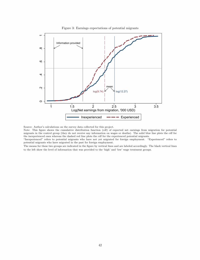
Figure 3: Earnings expectations of potential migrants

log(12.27)log(9.74)

mean

Information provided0

.2.4

.6.8

1

1 1.5 2 2.5 3 3.5Log(Net earnings from migration, '000 USD)

Inexperienced Experienced

Source: Author’s calculations on the survey data collected for this project.Note: This figure shows the cumulative distribution function (cdf) of expected net earnings from migration for potentialmigrants in the control group (they do not receive any information on wages or deaths). The solid blue line plots the cdf forthe inexperienced ones whereas the dashed red line plots the cdf for the experienced potential migrants.“Inexperienced” refers to potential migrants who have not yet migrated for foreign employment. “Experienced” refers topotential migrants who have migrated in the past for foreign employment.The means for these two groups are indicated in the figure by vertical lines and are labeled accordingly. The black vertical linesto the left show the level of information that was provided to the ‘high’ and ‘low’ wage treatment groups.

42

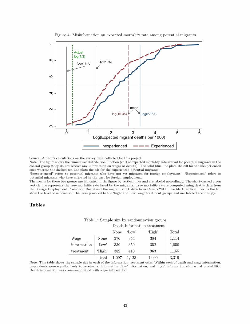
Figure 4: Misinformation on expected mortality rate among potential migrants

log(27.57)log(16.35)

Actuallog(1.3)

mean

'High' info'Low' info

0.2

.4.6

.81

0 1 2 3 4 5 6Log(Expected migrant deaths per 1000)

Inexperienced Experienced

Source: Author’s calculations on the survey data collected for this projectNote: The figure shows the cumulative distribution function (cdf) of expected mortality rate abroad for potential migrants in thecontrol group (they do not receive any information on wages or deaths). The solid blue line plots the cdf for the inexperiencedones whereas the dashed red line plots the cdf for the experienced potential migrants.“Inexperienced” refers to potential migrants who have not yet migrated for foreign employment. “Experienced” refers topotential migrants who have migrated in the past for foreign employment.The means for these two groups are indicated in the figure by vertical lines and are labeled accordingly. The short-dashed greenverticle line represents the true mortality rate faced by the migrants. True mortality rate is computed using deaths data fromthe Foreign Employment Promotion Board and the migrant stock data from Census 2011. The black vertical lines to the leftshow the level of information that was provided to the ‘high’ and ‘low’ wage treatment groups and are labeled accordingly.

Tables

Table 1: Sample size by randomization groupsDeath Information treatmentNone ‘Low’ ‘High’ Total

Wage None 376 354 384 1,114information ‘Low’ 339 359 352 1,050treatment ‘High’ 382 410 363 1,155

Total 1,097 1,123 1,099 3,319Note: This table shows the sample size in each of the information treatment cells. Within each of death and wage information,respondents were equally likely to receive no information, ‘low’ information, and ‘high’ information with equal probability.Death information was cross-randomized with wage information.

43

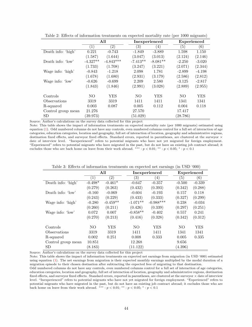
Table 2: Effects of information treatments on expected mortality rate (per 1000 migrants)All Inexperienced Experienced

(1) (2) (3) (4) (5) (6)Death info: ‘high’ 0.221 -0.743 -1.849 -3.889 1.598 1.150

(1.587) (1.644) (3.047) (3.013) (2.124) (2.146)Death info: ‘low’ -4.327** -4.843*** -7.413** -8.081** -2.250 -3.020

(1.733) (1.708) (3.247) (3.221) (2.071) (2.344)Wage info: ‘high’ -0.843 -1.218 2.098 1.781 -2.899 -4.198

(1.678) (1.680) (2.931) (3.179) (2.586) (2.812)Wage info: ‘low’ -0.626 -0.699 2.209 2.580 -3.125 -2.817

(1.843) (1.846) (2.991) (3.028) (2.889) (2.955)

Controls NO YES NO YES NO YESObservations 3319 3319 1411 1411 1341 1341R-squared 0.003 0.087 0.005 0.112 0.004 0.118Control group mean 21.276 27.570 17.417SD (39.973) (51.029) (28.786)

Source: Author’s calculations on the survey data collected for this projectNote: This table shows the impact of information treatments on expected mortality rate (per 1000 migrants) estimated usingequation (1). Odd numbered columns do not have any controls, even numbered columns control for a full set of interaction of agecategories, education categories, location and geography, full set of interaction of location, geography and administrative regions,destination fixed effects, and surveyor fixed effects. Standard errors, reported in parentheses, are clustered at the surveyor ×date of interview level. “Inexperienced” refers to potential migrants who have not yet migrated for foreign employment.“Experienced” refers to potential migrants who have migrated in the past, but do not have an existing job contract abroad; itexcludes those who are back home on leave from their work abroad. ∗∗∗ : p < 0.01; ∗∗ : p < 0.05; ∗ : p < 0.1

Table 3: Effects of information treatments on expected net earnings (in USD ‘000)All Inexperienced Experienced

(1) (2) (3) (4) (5) (6)Death info: ‘high’ -0.498* -0.461* -0.647 -0.357 -0.500 -0.339

(0.279) (0.263) (0.432) (0.393) (0.342) (0.288)Death info: ‘low’ -0.160 -0.069 -0.604 -0.193 0.157 0.118

(0.243) (0.229) (0.433) (0.333) (0.327) (0.299)Wage info: ‘high’ -0.280 -0.459** -1.071** -0.988*** 0.238 -0.034

(0.260) (0.211) (0.426) (0.339) (0.297) (0.251)Wage info: ‘low’ 0.072 0.007 -0.858** -0.402 0.557 0.241

(0.270) (0.213) (0.416) (0.328) (0.342) (0.312)

Controls NO YES NO YES NO YESObservations 3319 3319 1411 1411 1341 1341R-squared 0.002 0.251 0.008 0.333 0.005 0.335Control group mean 10.851 12.268 9.656SD (8.183) (11.122) (4.396)

Source: Author’s calculations on the survey data collected for this projectNote: This table shows the impact of information treatments on expected net earnings from migration (in USD ‘000) estimatedusing equation (1). The net earnings from migration is their expected monthly earnings multiplied by the modal duration of amigration episode to their chosen destnation after subtracting the expected fees of migrating to that destination.Odd numbered columns do not have any controls, even numbered columns control for a full set of interaction of age categories,education categories, location and geography, full set of interaction of location, geography and administrative regions, destinationfixed effects, and surveyor fixed effects. Standard errors, reported in parentheses, are clustered at the surveyor× date of interviewlevel. “Inexperienced” refers to potential migrants who have not yet migrated for foreign employment. “Experienced” refers topotential migrants who have migrated in the past, but do not have an existing job contract abroad; it excludes those who areback home on leave from their work abroad. ∗∗∗ : p < 0.01; ∗∗ : p < 0.05; ∗ : p < 0.1

44

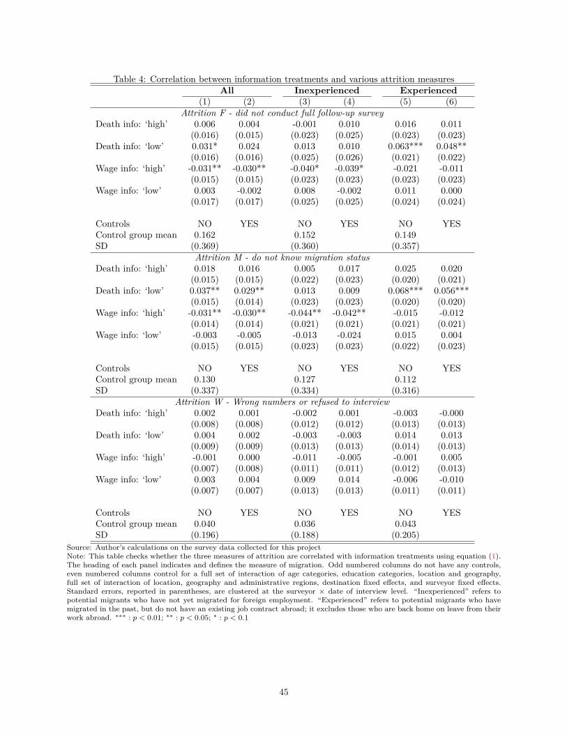
Table 4: Correlation between information treatments and various attrition measuresAll Inexperienced Experienced

(1) (2) (3) (4) (5) (6)Attrition F - did not conduct full follow-up survey

Death info: ‘high’ 0.006 0.004 -0.001 0.010 0.016 0.011(0.016) (0.015) (0.023) (0.025) (0.023) (0.023)

Death info: ‘low’ 0.031* 0.024 0.013 0.010 0.063*** 0.048**(0.016) (0.016) (0.025) (0.026) (0.021) (0.022)

Wage info: ‘high’ -0.031** -0.030** -0.040* -0.039* -0.021 -0.011(0.015) (0.015) (0.023) (0.023) (0.023) (0.023)

Wage info: ‘low’ 0.003 -0.002 0.008 -0.002 0.011 0.000(0.017) (0.017) (0.025) (0.025) (0.024) (0.024)

Controls NO YES NO YES NO YESControl group mean 0.162 0.152 0.149SD (0.369) (0.360) (0.357)

Attrition M - do not know migration statusDeath info: ‘high’ 0.018 0.016 0.005 0.017 0.025 0.020

(0.015) (0.015) (0.022) (0.023) (0.020) (0.021)Death info: ‘low’ 0.037** 0.029** 0.013 0.009 0.068*** 0.056***

(0.015) (0.014) (0.023) (0.023) (0.020) (0.020)Wage info: ‘high’ -0.031** -0.030** -0.044** -0.042** -0.015 -0.012

(0.014) (0.014) (0.021) (0.021) (0.021) (0.021)Wage info: ‘low’ -0.003 -0.005 -0.013 -0.024 0.015 0.004

(0.015) (0.015) (0.023) (0.023) (0.022) (0.023)

Controls NO YES NO YES NO YESControl group mean 0.130 0.127 0.112SD (0.337) (0.334) (0.316)

Attrition W - Wrong numbers or refused to interviewDeath info: ‘high’ 0.002 0.001 -0.002 0.001 -0.003 -0.000

(0.008) (0.008) (0.012) (0.012) (0.013) (0.013)Death info: ‘low’ 0.004 0.002 -0.003 -0.003 0.014 0.013

(0.009) (0.009) (0.013) (0.013) (0.014) (0.013)Wage info: ‘high’ -0.001 0.000 -0.011 -0.005 -0.001 0.005

(0.007) (0.008) (0.011) (0.011) (0.012) (0.013)Wage info: ‘low’ 0.003 0.004 0.009 0.014 -0.006 -0.010

(0.007) (0.007) (0.013) (0.013) (0.011) (0.011)

Controls NO YES NO YES NO YESControl group mean 0.040 0.036 0.043SD (0.196) (0.188) (0.205)

Source: Author’s calculations on the survey data collected for this projectNote: This table checks whether the three measures of attrition are correlated with information treatments using equation (1).The heading of each panel indicates and defines the measure of migration. Odd numbered columns do not have any controls,even numbered columns control for a full set of interaction of age categories, education categories, location and geography,full set of interaction of location, geography and administrative regions, destination fixed effects, and surveyor fixed effects.Standard errors, reported in parentheses, are clustered at the surveyor × date of interview level. “Inexperienced” refers topotential migrants who have not yet migrated for foreign employment. “Experienced” refers to potential migrants who havemigrated in the past, but do not have an existing job contract abroad; it excludes those who are back home on leave from theirwork abroad. ∗∗∗ : p < 0.01; ∗∗ : p < 0.05; ∗ : p < 0.1

45

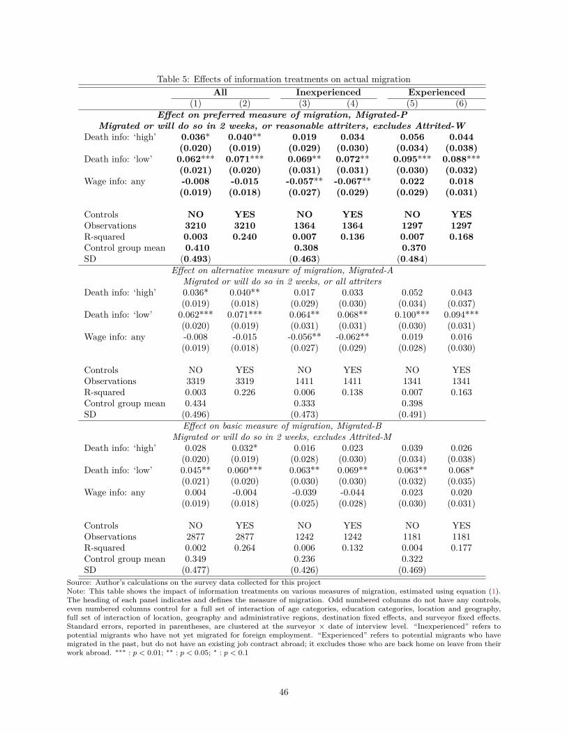
Table 5: Effects of information treatments on actual migrationAll Inexperienced Experienced

(1) (2) (3) (4) (5) (6)Effect on preferred measure of migration, Migrated-P

Migrated or will do so in 2 weeks, or reasonable attriters, excludes Attrited-WDeath info: ‘high’ 0.036* 0.040** 0.019 0.034 0.056 0.044

(0.020) (0.019) (0.029) (0.030) (0.034) (0.038)Death info: ‘low’ 0.062*** 0.071*** 0.069** 0.072** 0.095*** 0.088***

(0.021) (0.020) (0.031) (0.031) (0.030) (0.032)Wage info: any -0.008 -0.015 -0.057** -0.067** 0.022 0.018

(0.019) (0.018) (0.027) (0.029) (0.029) (0.031)

Controls NO YES NO YES NO YESObservations 3210 3210 1364 1364 1297 1297R-squared 0.003 0.240 0.007 0.136 0.007 0.168Control group mean 0.410 0.308 0.370SD (0.493) (0.463) (0.484)

Effect on alternative measure of migration, Migrated-AMigrated or will do so in 2 weeks, or all attriters

Death info: ‘high’ 0.036* 0.040** 0.017 0.033 0.052 0.043(0.019) (0.018) (0.029) (0.030) (0.034) (0.037)

Death info: ‘low’ 0.062*** 0.071*** 0.064** 0.068** 0.100*** 0.094***(0.020) (0.019) (0.031) (0.031) (0.030) (0.031)

Wage info: any -0.008 -0.015 -0.056** -0.062** 0.019 0.016(0.019) (0.018) (0.027) (0.029) (0.028) (0.030)

Controls NO YES NO YES NO YESObservations 3319 3319 1411 1411 1341 1341R-squared 0.003 0.226 0.006 0.138 0.007 0.163Control group mean 0.434 0.333 0.398SD (0.496) (0.473) (0.491)

Effect on basic measure of migration, Migrated-BMigrated or will do so in 2 weeks, excludes Attrited-M

Death info: ‘high’ 0.028 0.032* 0.016 0.023 0.039 0.026(0.020) (0.019) (0.028) (0.030) (0.034) (0.038)

Death info: ‘low’ 0.045** 0.060*** 0.063** 0.069** 0.063** 0.068*(0.021) (0.020) (0.030) (0.030) (0.032) (0.035)

Wage info: any 0.004 -0.004 -0.039 -0.044 0.023 0.020(0.019) (0.018) (0.025) (0.028) (0.030) (0.031)

Controls NO YES NO YES NO YESObservations 2877 2877 1242 1242 1181 1181R-squared 0.002 0.264 0.006 0.132 0.004 0.177Control group mean 0.349 0.236 0.322SD (0.477) (0.426) (0.469)

Source: Author’s calculations on the survey data collected for this projectNote: This table shows the impact of information treatments on various measures of migration, estimated using equation (1).The heading of each panel indicates and defines the measure of migration. Odd numbered columns do not have any controls,even numbered columns control for a full set of interaction of age categories, education categories, location and geography,full set of interaction of location, geography and administrative regions, destination fixed effects, and surveyor fixed effects.Standard errors, reported in parentheses, are clustered at the surveyor × date of interview level. “Inexperienced” refers topotential migrants who have not yet migrated for foreign employment. “Experienced” refers to potential migrants who havemigrated in the past, but do not have an existing job contract abroad; it excludes those who are back home on leave from theirwork abroad. ∗∗∗ : p < 0.01; ∗∗ : p < 0.05; ∗ : p < 0.1

46

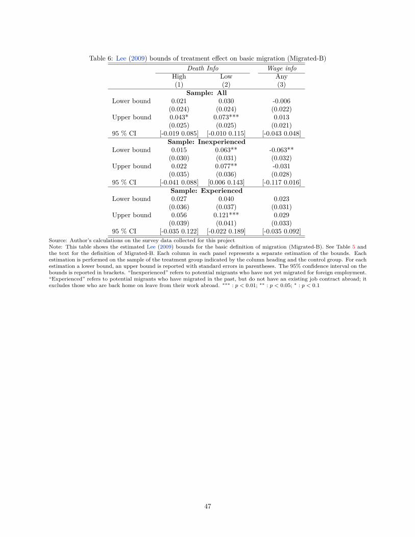
Table 6: Lee (2009) bounds of treatment effect on basic migration (Migrated-B)Death Info Wage info

High Low Any(1) (2) (3)

Sample: AllLower bound 0.021 0.030 -0.006

(0.024) (0.024) (0.022)Upper bound 0.043* 0.073*** 0.013

(0.025) (0.025) (0.021)95 % CI [-0.019 0.085] [-0.010 0.115] [-0.043 0.048]

Sample: InexperiencedLower bound 0.015 0.063** -0.063**

(0.030) (0.031) (0.032)Upper bound 0.022 0.077** -0.031

(0.035) (0.036) (0.028)95 % CI [-0.041 0.088] [0.006 0.143] [-0.117 0.016]

Sample: ExperiencedLower bound 0.027 0.040 0.023

(0.036) (0.037) (0.031)Upper bound 0.056 0.121*** 0.029

(0.039) (0.041) (0.033)95 % CI [-0.035 0.122] [-0.022 0.189] [-0.035 0.092]

Source: Author’s calculations on the survey data collected for this projectNote: This table shows the estimated Lee (2009) bounds for the basic definition of migration (Migrated-B). See Table 5 andthe text for the definition of Migrated-B. Each column in each panel represents a separate estimation of the bounds. Eachestimation is performed on the sample of the treatment group indicated by the column heading and the control group. For eachestimation a lower bound, an upper bound is reported with standard errors in parentheses. The 95% confidence interval on thebounds is reported in brackets. “Inexperienced” refers to potential migrants who have not yet migrated for foreign employment.“Experienced” refers to potential migrants who have migrated in the past, but do not have an existing job contract abroad; itexcludes those who are back home on leave from their work abroad. ∗∗∗ : p < 0.01; ∗∗ : p < 0.05; ∗ : p < 0.1

47

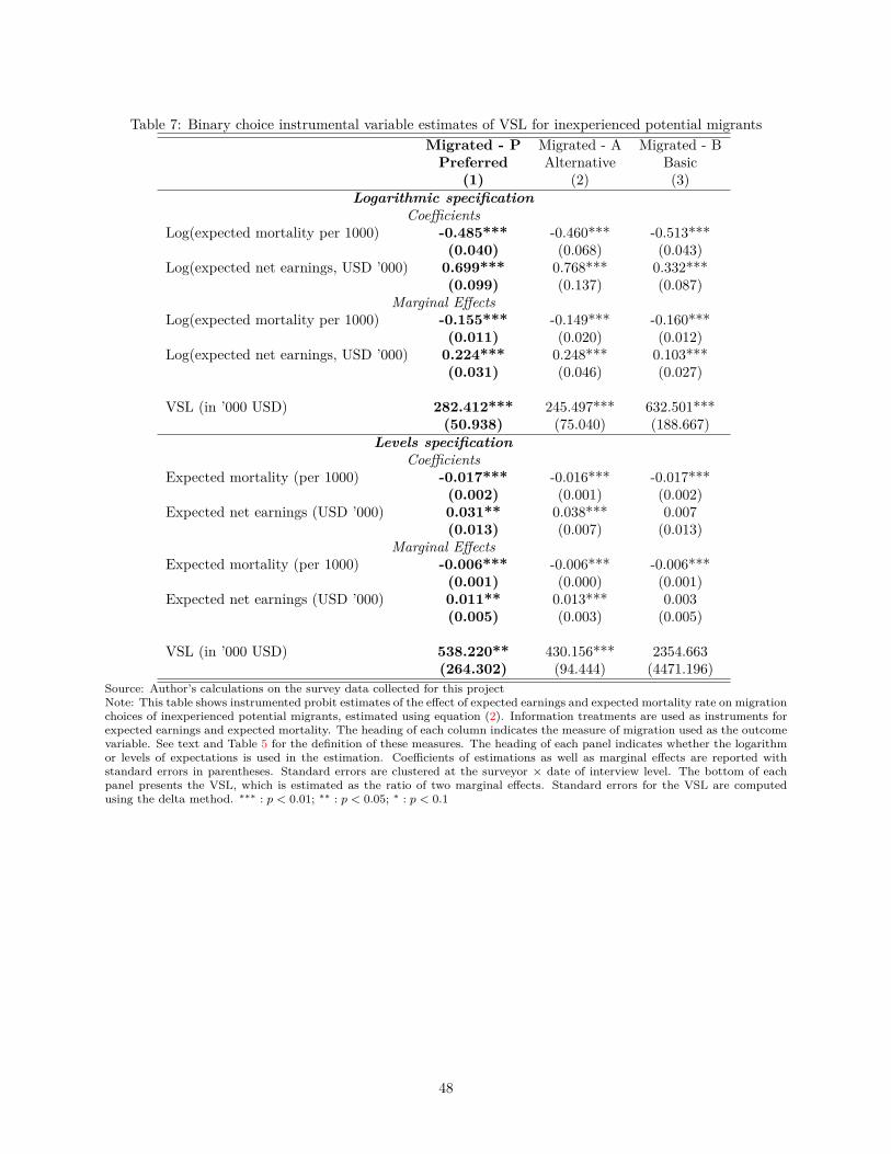
Table 7: Binary choice instrumental variable estimates of VSL for inexperienced potential migrantsMigrated - P Migrated - A Migrated - BPreferred Alternative Basic

(1) (2) (3)Logarithmic specification

CoefficientsLog(expected mortality per 1000) -0.485*** -0.460*** -0.513***

(0.040) (0.068) (0.043)Log(expected net earnings, USD ’000) 0.699*** 0.768*** 0.332***

(0.099) (0.137) (0.087)Marginal Effects

Log(expected mortality per 1000) -0.155*** -0.149*** -0.160***(0.011) (0.020) (0.012)

Log(expected net earnings, USD ’000) 0.224*** 0.248*** 0.103***(0.031) (0.046) (0.027)

VSL (in ’000 USD) 282.412*** 245.497*** 632.501***(50.938) (75.040) (188.667)

Levels specificationCoefficients

Expected mortality (per 1000) -0.017*** -0.016*** -0.017***(0.002) (0.001) (0.002)

Expected net earnings (USD ’000) 0.031** 0.038*** 0.007(0.013) (0.007) (0.013)

Marginal EffectsExpected mortality (per 1000) -0.006*** -0.006*** -0.006***

(0.001) (0.000) (0.001)Expected net earnings (USD ’000) 0.011** 0.013*** 0.003

(0.005) (0.003) (0.005)

VSL (in ’000 USD) 538.220** 430.156*** 2354.663(264.302) (94.444) (4471.196)

Source: Author’s calculations on the survey data collected for this projectNote: This table shows instrumented probit estimates of the effect of expected earnings and expected mortality rate on migrationchoices of inexperienced potential migrants, estimated using equation (2). Information treatments are used as instruments forexpected earnings and expected mortality. The heading of each column indicates the measure of migration used as the outcomevariable. See text and Table 5 for the definition of these measures. The heading of each panel indicates whether the logarithmor levels of expectations is used in the estimation. Coefficients of estimations as well as marginal effects are reported withstandard errors in parentheses. Standard errors are clustered at the surveyor × date of interview level. The bottom of eachpanel presents the VSL, which is estimated as the ratio of two marginal effects. Standard errors for the VSL are computedusing the delta method. ∗∗∗ : p < 0.01; ∗∗ : p < 0.05; ∗ : p < 0.1

48

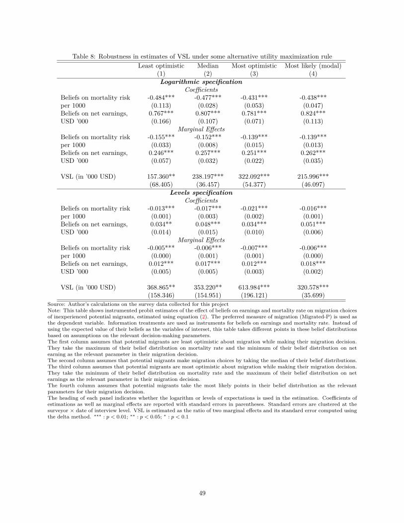
Table 8: Robustness in estimates of VSL under some alternative utility maximization ruleLeast optimistic Median Most optimistic Most likely (modal)

(1) (2) (3) (4)Logarithmic specification

CoefficientsBeliefs on mortality risk -0.484*** -0.477*** -0.431*** -0.438***per 1000 (0.113) (0.028) (0.053) (0.047)Beliefs on net earnings, 0.767*** 0.807*** 0.781*** 0.824***USD ’000 (0.166) (0.107) (0.071) (0.113)

Marginal EffectsBeliefs on mortality risk -0.155*** -0.152*** -0.139*** -0.139***per 1000 (0.033) (0.008) (0.015) (0.013)Beliefs on net earnings, 0.246*** 0.257*** 0.251*** 0.262***USD ’000 (0.057) (0.032) (0.022) (0.035)

VSL (in ’000 USD) 157.360** 238.197*** 322.092*** 215.996***(68.405) (36.457) (54.377) (46.097)

Levels specificationCoefficients

Beliefs on mortality risk -0.013*** -0.017*** -0.021*** -0.016***per 1000 (0.001) (0.003) (0.002) (0.001)Beliefs on net earnings, 0.034** 0.048*** 0.034*** 0.051***USD ’000 (0.014) (0.015) (0.010) (0.006)

Marginal EffectsBeliefs on mortality risk -0.005*** -0.006*** -0.007*** -0.006***per 1000 (0.000) (0.001) (0.001) (0.000)Beliefs on net earnings, 0.012*** 0.017*** 0.012*** 0.018***USD ’000 (0.005) (0.005) (0.003) (0.002)

VSL (in ’000 USD) 368.865** 353.220** 613.984*** 320.578***(158.346) (154.951) (196.121) (35.699)

Source: Author’s calculations on the survey data collected for this projectNote: This table shows instrumented probit estimates of the effect of beliefs on earnings and mortality rate on migration choicesof inexperienced potential migrants, estimated using equation (2). The preferred measure of migration (Migrated-P) is used asthe dependent variable. Information treatments are used as instruments for beliefs on earnings and mortality rate. Instead ofusing the expected value of their beliefs as the variables of interset, this table takes different points in these belief distributionsbased on assumptions on the relevant decision-making parameters.The first column assumes that potential migrants are least optimistic about migration while making their migration decision.They take the maximum of their belief distribution on mortality rate and the minimum of their belief distribution on netearning as the relevant parameter in their migration decision.The second column assumes that potential migrants make migration choices by taking the median of their belief distributions.The third column assumes that potential migrants are most optimistic about migration while making their migration decision.They take the minimum of their belief distribution on mortality rate and the maximum of their belief distribution on netearnings as the relevant parameter in their migration decision.The fourth column assumes that potential migrants take the most likely points in their belief distribution as the relevantparameters for their migration decision.The heading of each panel indicates whether the logarithm or levels of expectations is used in the estimation. Coefficients ofestimations as well as marginal effects are reported with standard errors in parentheses. Standard errors are clustered at thesurveyor × date of interview level. VSL is estimated as the ratio of two marginal effects and its standard error computed usingthe delta method. ∗∗∗ : p < 0.01; ∗∗ : p < 0.05; ∗ : p < 0.1

49

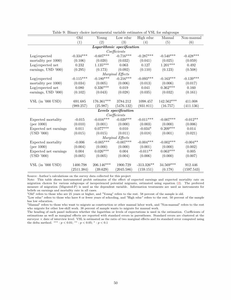
Table 9: Binary choice instrumental variable estimates of VSL for subgroupsOld Young Low educ High educ Manual Non-manual(1) (2) (3) (4) (5) (6)

Logarithmic specificationCoefficients

Log(expected -0.334*** -0.607*** -0.716*** -0.287*** -0.540*** -0.428***mortality per 1000) (0.106) (0.020) (0.032) (0.041) (0.025) (0.059)Log(expected net 0.232 1.135*** 0.063 0.127 1.201*** 0.492earnings, USD ’000) (0.295) (0.173) (0.092) (0.110) (0.123) (0.508)

Marginal EffectsLog(expected -0.115*** -0.180*** -0.216*** -0.093*** -0.163*** -0.139***mortality per 1000) (0.034) (0.005) (0.006) (0.013) (0.006) (0.017)Log(expected net 0.080 0.336*** 0.019 0.041 0.362*** 0.160earnings, USD ’000) (0.102) (0.043) (0.028) (0.035) (0.032) (0.161)

VSL (in ’000 USD) 691.685 176.361*** 3784.212 1098.457 142.562*** 411.008(989.257) (25.987) (5476.132) (931.811) (16.757) (411.136)

Levels specificationCoefficients

Expected mortality -0.015 -0.016*** -0.020*** -0.011*** -0.007*** -0.012**(per 1000) (0.010) (0.001) (0.000) (0.003) (0.000) (0.006)Expected net earnings 0.011 0.077*** 0.010 -0.034* 0.209*** 0.014(USD ’000) (0.015) (0.015) (0.011) (0.018) (0.001) (0.021)

Marginal EffectsExpected mortality -0.006 -0.005*** -0.007*** -0.004*** -0.002*** -0.004**(per 1000) (0.004) (0.000) (0.000) (0.001) (0.000) (0.002)Expected net earnings 0.004 0.026*** 0.004 -0.011** 0.063*** 0.005(USD ’000) (0.005) (0.005) (0.004) (0.006) (0.000) (0.007)

VSL (in ’000 USD) 1400.798 206.146*** 1900.729 -313.326** 34.569*** 912.446(2511.384) (39.629) (2045.586) (159.151) (0.178) (1597.543)

Source: Author’s calculations on the survey data collected for this projectNote: This table shows instrumented probit estimates of the effect of expected earnings and expected mortality rate onmigration choices for various subgroups of inexperienced potential migrants, estimated using equation (2). The preferredmeasure of migration (Migrated-P) is used as the dependent variable. Information treatments are used as instruments forbeliefs on earnings and mortality rate in all cases."Old" refers to those who are 21 years or higher, and "Young" refers to the rest. 58 percent of the sample is old."Low educ" refers to those who have 8 or fewer years of schooling, and "High educ" refers to the rest. 50 percent of the samplehas low education."Manual" refers to those who want to migrate as construction or other manual labor work, and "Non-manual" refers to the restwho migrate for other low-skill work. 38 percent of sample wants to migrate for manual work.The heading of each panel indicates whether the logarithm or levels of expectations is used in the estimation. Coefficients ofestimations as well as marginal effects are reported with standard errors in parentheses. Standard errors are clustered at thesurveyor × date of interview level. VSL is estimated as the ratio of two marginal effects and its standard error computed usingthe delta method. ∗∗∗ : p < 0.01; ∗∗ : p < 0.05; ∗ : p < 0.1

50

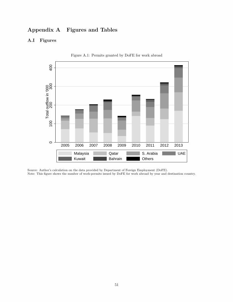
Appendix A Figures and Tables

A.I Figures

Figure A.1: Permits granted by DoFE for work abroad0

100

200

300

400

Tot

al o

utflo

w in

'000

2005 2006 2007 2008 2009 2010 2011 2012 2013

Malaysia Qatar S. Arabia UAEKuwait Bahrain Others

Source: Author’s calculation on the data provided by Department of Foreign Employment (DoFE).Note: This figure shows the number of work-permits issued by DoFE for work abroad by year and destination country.

51

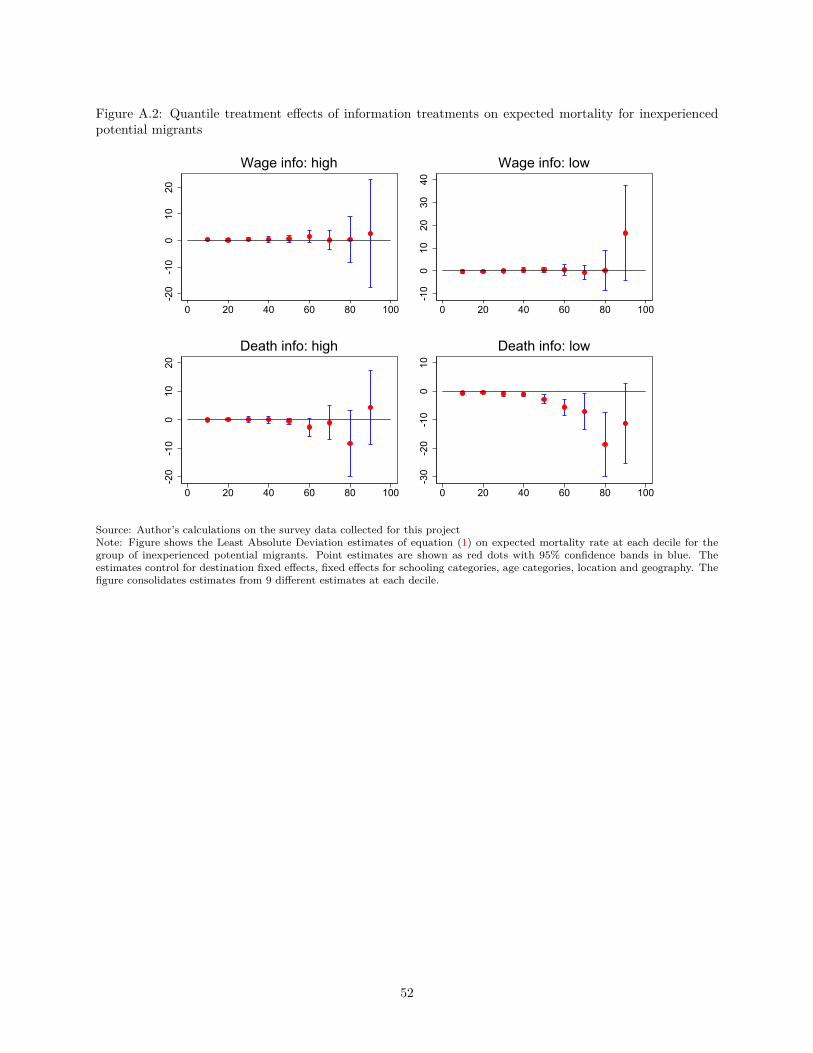
Figure A.2: Quantile treatment effects of information treatments on expected mortality for inexperiencedpotential migrants

-20

-10

010

20

0 20 40 60 80 100

Wage info: high

-10

010

2030

40

0 20 40 60 80 100

Wage info: low-2

0-1

00

1020

0 20 40 60 80 100

Death info: high

-30

-20

-10

010

0 20 40 60 80 100

Death info: low

Source: Author’s calculations on the survey data collected for this projectNote: Figure shows the Least Absolute Deviation estimates of equation (1) on expected mortality rate at each decile for thegroup of inexperienced potential migrants. Point estimates are shown as red dots with 95% confidence bands in blue. Theestimates control for destination fixed effects, fixed effects for schooling categories, age categories, location and geography. Thefigure consolidates estimates from 9 different estimates at each decile.

52

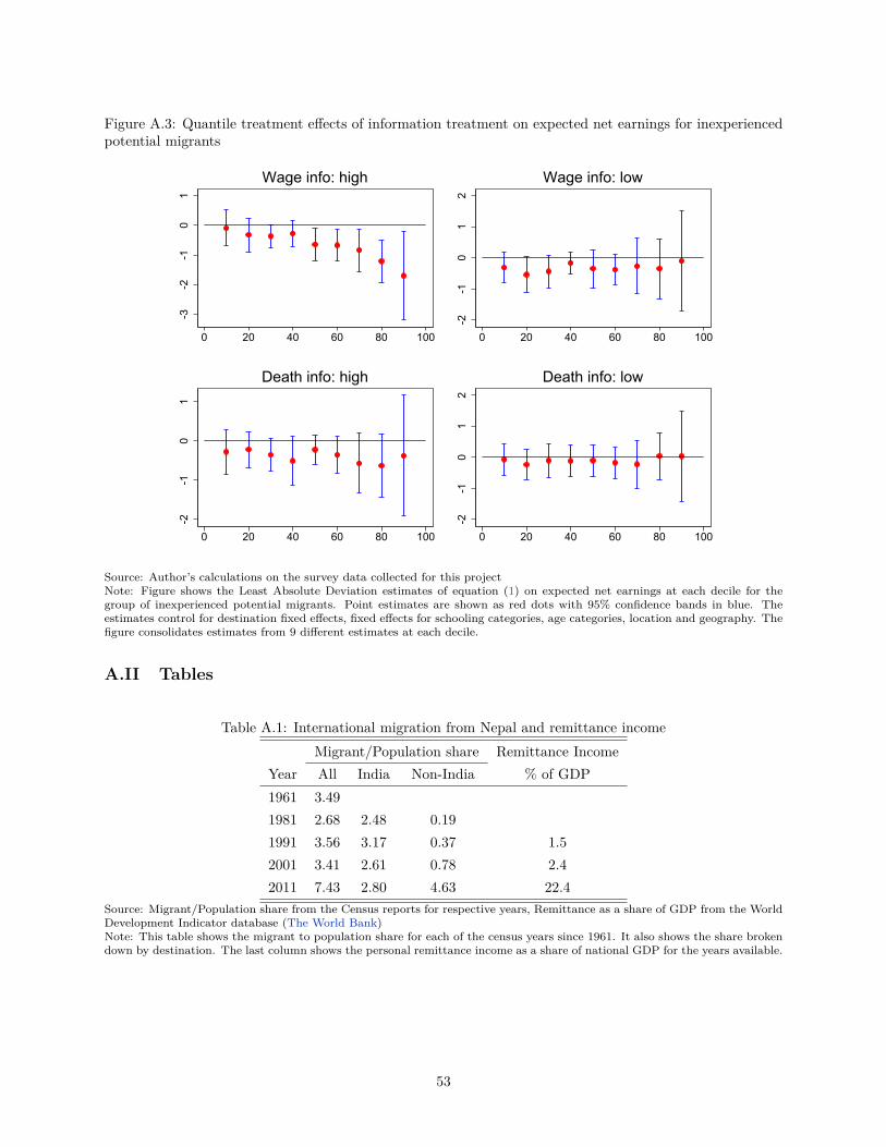
Figure A.3: Quantile treatment effects of information treatment on expected net earnings for inexperiencedpotential migrants

-3-2

-10

1

0 20 40 60 80 100

Wage info: high

-2-1

01

2

0 20 40 60 80 100

Wage info: low-2

-10

1

0 20 40 60 80 100

Death info: high

-2-1

01

2

0 20 40 60 80 100

Death info: low

Source: Author’s calculations on the survey data collected for this projectNote: Figure shows the Least Absolute Deviation estimates of equation (1) on expected net earnings at each decile for thegroup of inexperienced potential migrants. Point estimates are shown as red dots with 95% confidence bands in blue. Theestimates control for destination fixed effects, fixed effects for schooling categories, age categories, location and geography. Thefigure consolidates estimates from 9 different estimates at each decile.

A.II Tables

Table A.1: International migration from Nepal and remittance incomeMigrant/Population share Remittance Income

Year All India Non-India % of GDP1961 3.491981 2.68 2.48 0.191991 3.56 3.17 0.37 1.52001 3.41 2.61 0.78 2.42011 7.43 2.80 4.63 22.4

Source: Migrant/Population share from the Census reports for respective years, Remittance as a share of GDP from the WorldDevelopment Indicator database (The World Bank)Note: This table shows the migrant to population share for each of the census years since 1961. It also shows the share brokendown by destination. The last column shows the personal remittance income as a share of national GDP for the years available.

53

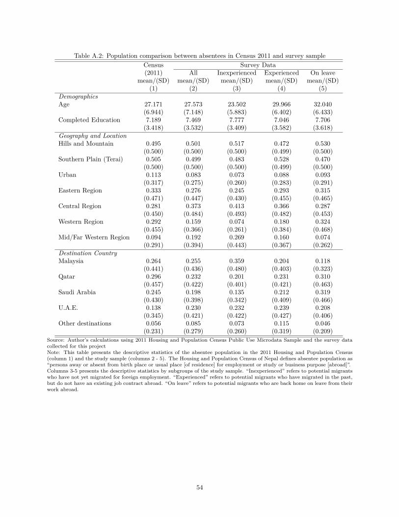
Table A.2: Population comparison between absentees in Census 2011 and survey sampleCensus Survey Data(2011) All Inexperienced Experienced On leave

mean/(SD) mean/(SD) mean/(SD) mean/(SD) mean/(SD)(1) (2) (3) (4) (5)

DemographicsAge 27.171 27.573 23.502 29.966 32.040

(6.944) (7.148) (5.883) (6.402) (6.433)Completed Education 7.189 7.469 7.777 7.046 7.706

(3.418) (3.532) (3.409) (3.582) (3.618)Geography and LocationHills and Mountain 0.495 0.501 0.517 0.472 0.530

(0.500) (0.500) (0.500) (0.499) (0.500)Southern Plain (Terai) 0.505 0.499 0.483 0.528 0.470

(0.500) (0.500) (0.500) (0.499) (0.500)Urban 0.113 0.083 0.073 0.088 0.093

(0.317) (0.275) (0.260) (0.283) (0.291)Eastern Region 0.333 0.276 0.245 0.293 0.315

(0.471) (0.447) (0.430) (0.455) (0.465)Central Region 0.281 0.373 0.413 0.366 0.287

(0.450) (0.484) (0.493) (0.482) (0.453)Western Region 0.292 0.159 0.074 0.180 0.324

(0.455) (0.366) (0.261) (0.384) (0.468)Mid/Far Western Region 0.094 0.192 0.269 0.160 0.074

(0.291) (0.394) (0.443) (0.367) (0.262)Destination CountryMalaysia 0.264 0.255 0.359 0.204 0.118

(0.441) (0.436) (0.480) (0.403) (0.323)Qatar 0.296 0.232 0.201 0.231 0.310

(0.457) (0.422) (0.401) (0.421) (0.463)Saudi Arabia 0.245 0.198 0.135 0.212 0.319

(0.430) (0.398) (0.342) (0.409) (0.466)U.A.E. 0.138 0.230 0.232 0.239 0.208

(0.345) (0.421) (0.422) (0.427) (0.406)Other destinations 0.056 0.085 0.073 0.115 0.046

(0.231) (0.279) (0.260) (0.319) (0.209)Source: Author’s calculations using 2011 Housing and Population Census Public Use Microdata Sample and the survey datacollected for this projectNote: This table presents the descriptive statistics of the absentee population in the 2011 Housing and Population Census(column 1) and the study sample (columns 2 - 5). The Housing and Population Census of Nepal defines absentee population as“persons away or absent from birth place or usual place [of residence] for employment or study or business purpose [abroad]”.Columns 3-5 presents the descriptive statistics by subgroups of the study sample. “Inexperienced” refers to potential migrantswho have not yet migrated for foreign employment. “Experienced” refers to potential migrants who have migrated in the past,but do not have an existing job contract abroad. “On leave” refers to potential migrants who are back home on leave from theirwork abroad.

54

Table A.3: Description of information provided to the subjectsDestination Countries

Malaysia Qatar Saudi Arabia U.A.E KuwaitMonthly flow 14,100 8,300 6,500 4,200 700Wage ‘High’ (NPR) 24,500 25,000 23,000 26,000 26,500Wage ‘Low’ (NPR) 12,500 15,500 13,500 19,000 15,000Death ‘High’ 9 8 9 3 2Death ‘Low’ 2 1 2 1 1

Note: This table presents the exact nature of information provided to the participants. Each row lists the information providedin each of the treatment groups for potential migrants to the Destination countries listed in the columns. Monthly flow is theaverage number of work-reated migrants leaving Nepal every month in 2013. Wage information is provided as monthly wagesin Nepali Rupees (exchange rate US$ 1= NPR 100). Death information provided indicates the number of deaths that occuredin a pre-determined district in 2013.

55

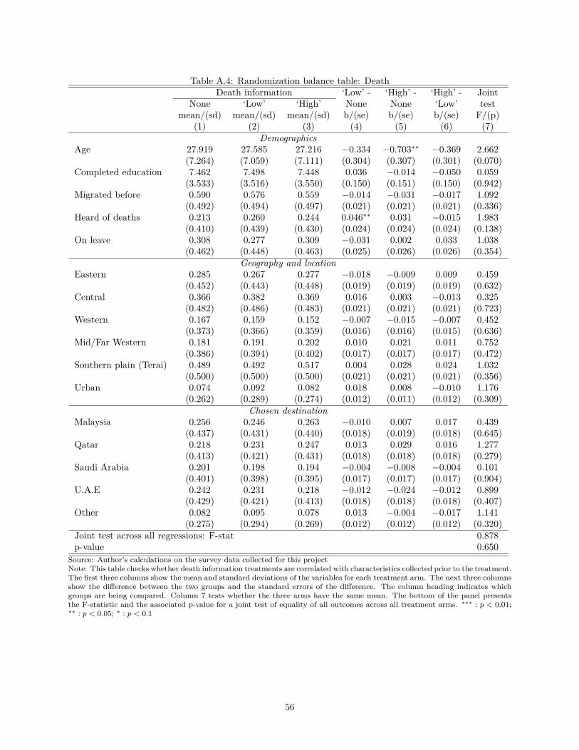
Table A.4: Randomization balance table: DeathDeath information ‘Low’ - ‘High’ - ‘High’ - Joint

None ‘Low’ ‘High’ None None ‘Low’ testmean/(sd) mean/(sd) mean/(sd) b/(se) b/(se) b/(se) F/(p)

(1) (2) (3) (4) (5) (6) (7)Demographics

Age 27.919 27.585 27.216 −0.334 −0.703∗∗ −0.369 2.662(7.264) (7.059) (7.111) (0.304) (0.307) (0.301) (0.070)

Completed education 7.462 7.498 7.448 0.036 −0.014 −0.050 0.059(3.533) (3.516) (3.550) (0.150) (0.151) (0.150) (0.942)

Migrated before 0.590 0.576 0.559 −0.014 −0.031 −0.017 1.092(0.492) (0.494) (0.497) (0.021) (0.021) (0.021) (0.336)

Heard of deaths 0.213 0.260 0.244 0.046∗∗ 0.031 −0.015 1.983(0.410) (0.439) (0.430) (0.024) (0.024) (0.024) (0.138)

On leave 0.308 0.277 0.309 −0.031 0.002 0.033 1.038(0.462) (0.448) (0.463) (0.025) (0.026) (0.026) (0.354)

Geography and locationEastern 0.285 0.267 0.277 −0.018 −0.009 0.009 0.459

(0.452) (0.443) (0.448) (0.019) (0.019) (0.019) (0.632)Central 0.366 0.382 0.369 0.016 0.003 −0.013 0.325

(0.482) (0.486) (0.483) (0.021) (0.021) (0.021) (0.723)Western 0.167 0.159 0.152 −0.007 −0.015 −0.007 0.452

(0.373) (0.366) (0.359) (0.016) (0.016) (0.015) (0.636)Mid/Far Western 0.181 0.191 0.202 0.010 0.021 0.011 0.752

(0.386) (0.394) (0.402) (0.017) (0.017) (0.017) (0.472)Southern plain (Terai) 0.489 0.492 0.517 0.004 0.028 0.024 1.032

(0.500) (0.500) (0.500) (0.021) (0.021) (0.021) (0.356)Urban 0.074 0.092 0.082 0.018 0.008 −0.010 1.176

(0.262) (0.289) (0.274) (0.012) (0.011) (0.012) (0.309)Chosen destination

Malaysia 0.256 0.246 0.263 −0.010 0.007 0.017 0.439(0.437) (0.431) (0.440) (0.018) (0.019) (0.018) (0.645)

Qatar 0.218 0.231 0.247 0.013 0.029 0.016 1.277(0.413) (0.421) (0.431) (0.018) (0.018) (0.018) (0.279)

Saudi Arabia 0.201 0.198 0.194 −0.004 −0.008 −0.004 0.101(0.401) (0.398) (0.395) (0.017) (0.017) (0.017) (0.904)

U.A.E 0.242 0.231 0.218 −0.012 −0.024 −0.012 0.899(0.429) (0.421) (0.413) (0.018) (0.018) (0.018) (0.407)

Other 0.082 0.095 0.078 0.013 −0.004 −0.017 1.141(0.275) (0.294) (0.269) (0.012) (0.012) (0.012) (0.320)

Joint test across all regressions: F-stat 0.878p-value 0.650

Source: Author’s calculations on the survey data collected for this projectNote: This table checks whether death information treatments are correlated with characteristics collected prior to the treatment.The first three columns show the mean and standard deviations of the variables for each treatment arm. The next three columnsshow the difference between the two groups and the standard errors of the difference. The column heading indicates whichgroups are being compared. Column 7 tests whether the three arms have the same mean. The bottom of the panel presentsthe F-statistic and the associated p-value for a joint test of equality of all outcomes across all treatment arms. ∗∗∗ : p < 0.01;∗∗ : p < 0.05; ∗ : p < 0.1

56

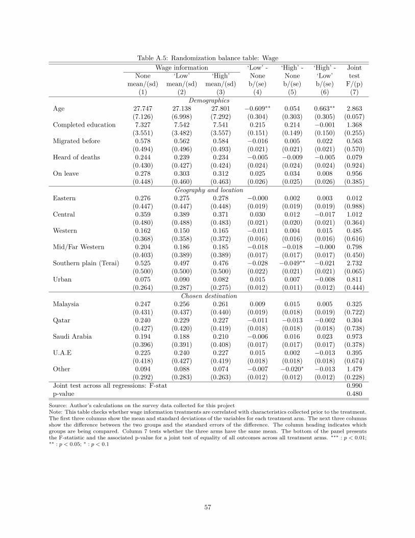
Table A.5: Randomization balance table: WageWage information ‘Low’ - ‘High’ - ‘High’ - Joint

None ‘Low’ ‘High’ None None ‘Low’ testmean/(sd) mean/(sd) mean/(sd) b/(se) b/(se) b/(se) F/(p)

(1) (2) (3) (4) (5) (6) (7)Demographics

Age 27.747 27.138 27.801 −0.609∗∗ 0.054 0.663∗∗ 2.863(7.126) (6.998) (7.292) (0.304) (0.303) (0.305) (0.057)

Completed education 7.327 7.542 7.541 0.215 0.214 −0.001 1.368(3.551) (3.482) (3.557) (0.151) (0.149) (0.150) (0.255)

Migrated before 0.578 0.562 0.584 −0.016 0.005 0.022 0.563(0.494) (0.496) (0.493) (0.021) (0.021) (0.021) (0.570)

Heard of deaths 0.244 0.239 0.234 −0.005 −0.009 −0.005 0.079(0.430) (0.427) (0.424) (0.024) (0.024) (0.024) (0.924)

On leave 0.278 0.303 0.312 0.025 0.034 0.008 0.956(0.448) (0.460) (0.463) (0.026) (0.025) (0.026) (0.385)

Geography and locationEastern 0.276 0.275 0.278 −0.000 0.002 0.003 0.012

(0.447) (0.447) (0.448) (0.019) (0.019) (0.019) (0.988)Central 0.359 0.389 0.371 0.030 0.012 −0.017 1.012

(0.480) (0.488) (0.483) (0.021) (0.020) (0.021) (0.364)Western 0.162 0.150 0.165 −0.011 0.004 0.015 0.485

(0.368) (0.358) (0.372) (0.016) (0.016) (0.016) (0.616)Mid/Far Western 0.204 0.186 0.185 −0.018 −0.018 −0.000 0.798

(0.403) (0.389) (0.389) (0.017) (0.017) (0.017) (0.450)Southern plain (Terai) 0.525 0.497 0.476 −0.028 −0.049∗∗ −0.021 2.732

(0.500) (0.500) (0.500) (0.022) (0.021) (0.021) (0.065)Urban 0.075 0.090 0.082 0.015 0.007 −0.008 0.811

(0.264) (0.287) (0.275) (0.012) (0.011) (0.012) (0.444)Chosen destination

Malaysia 0.247 0.256 0.261 0.009 0.015 0.005 0.325(0.431) (0.437) (0.440) (0.019) (0.018) (0.019) (0.722)

Qatar 0.240 0.229 0.227 −0.011 −0.013 −0.002 0.304(0.427) (0.420) (0.419) (0.018) (0.018) (0.018) (0.738)

Saudi Arabia 0.194 0.188 0.210 −0.006 0.016 0.023 0.973(0.396) (0.391) (0.408) (0.017) (0.017) (0.017) (0.378)

U.A.E 0.225 0.240 0.227 0.015 0.002 −0.013 0.395(0.418) (0.427) (0.419) (0.018) (0.018) (0.018) (0.674)

Other 0.094 0.088 0.074 −0.007 −0.020∗ −0.013 1.479(0.292) (0.283) (0.263) (0.012) (0.012) (0.012) (0.228)

Joint test across all regressions: F-stat 0.990p-value 0.480

Source: Author’s calculations on the survey data collected for this projectNote: This table checks whether wage information treatments are correlated with characteristics collected prior to the treatment.The first three columns show the mean and standard deviations of the variables for each treatment arm. The next three columnsshow the difference between the two groups and the standard errors of the difference. The column heading indicates whichgroups are being compared. Column 7 tests whether the three arms have the same mean. The bottom of the panel presentsthe F-statistic and the associated p-value for a joint test of equality of all outcomes across all treatment arms. ∗∗∗ : p < 0.01;∗∗ : p < 0.05; ∗ : p < 0.1

57

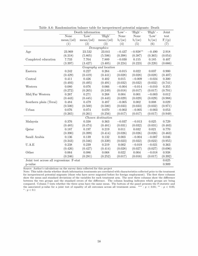
Table A.6: Randomization balance table for inexperienced potential migrants: DeathDeath information ‘Low’ - ‘High’ - ‘High’ - Joint

None ‘Low’ ‘High’ None None ‘Low’ testmean/(sd) mean/(sd) mean/(sd) b/(se) b/(se) b/(se) F/(p)

(1) (2) (3) (4) (5) (6) (7)Demographics

Age 23.969 23.532 23.041 −0.437 −0.928∗∗ −0.490 2.918(6.318) (5.805) (5.506) (0.398) (0.387) (0.365) (0.054)

Completed education 7.733 7.704 7.889 −0.030 0.155 0.185 0.407(3.397) (3.427) (3.405) (0.224) (0.223) (0.220) (0.666)

Geography and locationEastern 0.242 0.227 0.264 −0.015 0.022 0.037 0.900

(0.429) (0.419) (0.441) (0.028) (0.028) (0.028) (0.407)Central 0.411 0.426 0.402 0.015 −0.009 −0.024 0.300

(0.493) (0.495) (0.491) (0.032) (0.032) (0.032) (0.741)Western 0.080 0.076 0.066 −0.004 −0.014 −0.010 0.355

(0.272) (0.265) (0.249) (0.018) (0.017) (0.017) (0.701)Mid/Far Western 0.267 0.271 0.268 0.004 0.001 −0.003 0.012

(0.443) (0.445) (0.443) (0.029) (0.029) (0.029) (0.988)Southern plain (Terai) 0.484 0.479 0.487 −0.005 0.002 0.008 0.029

(0.500) (0.500) (0.500) (0.033) (0.033) (0.032) (0.971)Urban 0.076 0.074 0.070 −0.002 −0.005 −0.003 0.053

(0.265) (0.261) (0.256) (0.017) (0.017) (0.017) (0.949)Chosen destination

Malaysia 0.376 0.338 0.363 −0.037 −0.013 0.025 0.729(0.485) (0.474) (0.481) (0.031) (0.032) (0.031) (0.483)

Qatar 0.187 0.197 0.219 0.011 0.032 0.021 0.770(0.390) (0.399) (0.414) (0.026) (0.026) (0.026) (0.463)

Saudi Arabia 0.136 0.139 0.132 0.003 −0.004 −0.007 0.046(0.343) (0.346) (0.339) (0.023) (0.022) (0.022) (0.955)

U.A.E 0.238 0.239 0.219 0.002 −0.019 −0.021 0.363(0.426) (0.427) (0.414) (0.028) (0.027) (0.027) (0.696)

Other 0.064 0.086 0.068 0.022 0.004 −0.018 0.938(0.246) (0.281) (0.252) (0.017) (0.016) (0.017) (0.392)

Joint test across all regressions: F-stat 0.625p-value 0.909

Source: Author’s calculations on the survey data collected for this projectNote: This table checks whether death information treatments are correlated with characteristics collected prior to the treatmentfor inexperienced potential migrants (those who have never migrated before for foreign employment). The first three columnsshow the mean and standard deviations of the variables for each treatment arm. The next three columns show the differencebetween the two groups and the standard errors of the difference. The column heading indicates which groups are beingcompared. Column 7 tests whether the three arms have the same mean. The bottom of the panel presents the F-statistic andthe associated p-value for a joint test of equality of all outcomes across all treatment arms. ∗∗∗ : p < 0.01; ∗∗ : p < 0.05;∗ : p < 0.1

58

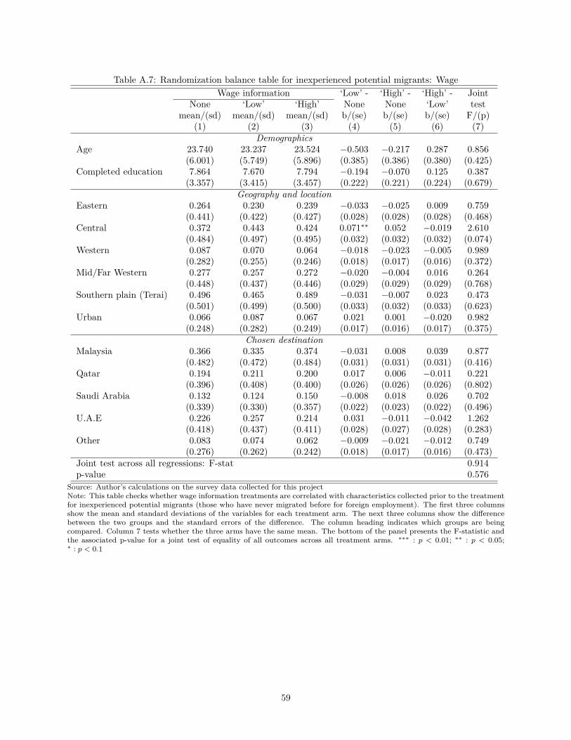
Table A.7: Randomization balance table for inexperienced potential migrants: WageWage information ‘Low’ - ‘High’ - ‘High’ - Joint

None ‘Low’ ‘High’ None None ‘Low’ testmean/(sd) mean/(sd) mean/(sd) b/(se) b/(se) b/(se) F/(p)

(1) (2) (3) (4) (5) (6) (7)Demographics

Age 23.740 23.237 23.524 −0.503 −0.217 0.287 0.856(6.001) (5.749) (5.896) (0.385) (0.386) (0.380) (0.425)

Completed education 7.864 7.670 7.794 −0.194 −0.070 0.125 0.387(3.357) (3.415) (3.457) (0.222) (0.221) (0.224) (0.679)

Geography and locationEastern 0.264 0.230 0.239 −0.033 −0.025 0.009 0.759

(0.441) (0.422) (0.427) (0.028) (0.028) (0.028) (0.468)Central 0.372 0.443 0.424 0.071∗∗ 0.052 −0.019 2.610

(0.484) (0.497) (0.495) (0.032) (0.032) (0.032) (0.074)Western 0.087 0.070 0.064 −0.018 −0.023 −0.005 0.989

(0.282) (0.255) (0.246) (0.018) (0.017) (0.016) (0.372)Mid/Far Western 0.277 0.257 0.272 −0.020 −0.004 0.016 0.264

(0.448) (0.437) (0.446) (0.029) (0.029) (0.029) (0.768)Southern plain (Terai) 0.496 0.465 0.489 −0.031 −0.007 0.023 0.473

(0.501) (0.499) (0.500) (0.033) (0.032) (0.033) (0.623)Urban 0.066 0.087 0.067 0.021 0.001 −0.020 0.982

(0.248) (0.282) (0.249) (0.017) (0.016) (0.017) (0.375)Chosen destination

Malaysia 0.366 0.335 0.374 −0.031 0.008 0.039 0.877(0.482) (0.472) (0.484) (0.031) (0.031) (0.031) (0.416)

Qatar 0.194 0.211 0.200 0.017 0.006 −0.011 0.221(0.396) (0.408) (0.400) (0.026) (0.026) (0.026) (0.802)

Saudi Arabia 0.132 0.124 0.150 −0.008 0.018 0.026 0.702(0.339) (0.330) (0.357) (0.022) (0.023) (0.022) (0.496)

U.A.E 0.226 0.257 0.214 0.031 −0.011 −0.042 1.262(0.418) (0.437) (0.411) (0.028) (0.027) (0.028) (0.283)

Other 0.083 0.074 0.062 −0.009 −0.021 −0.012 0.749(0.276) (0.262) (0.242) (0.018) (0.017) (0.016) (0.473)

Joint test across all regressions: F-stat 0.914p-value 0.576

Source: Author’s calculations on the survey data collected for this projectNote: This table checks whether wage information treatments are correlated with characteristics collected prior to the treatmentfor inexperienced potential migrants (those who have never migrated before for foreign employment). The first three columnsshow the mean and standard deviations of the variables for each treatment arm. The next three columns show the differencebetween the two groups and the standard errors of the difference. The column heading indicates which groups are beingcompared. Column 7 tests whether the three arms have the same mean. The bottom of the panel presents the F-statistic andthe associated p-value for a joint test of equality of all outcomes across all treatment arms. ∗∗∗ : p < 0.01; ∗∗ : p < 0.05;∗ : p < 0.1

59

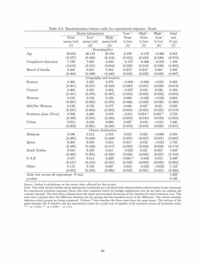
Table A.8: Randomization balance table for experienced migrants: DeathDeath information ‘Low’ - ‘High’ - ‘High’ - Joint

None ‘Low’ ‘High’ None None ‘Low’ testmean/(sd) mean/(sd) mean/(sd) b/(se) b/(se) b/(se) F/(p)

(1) (2) (3) (4) (5) (6) (7)Demographics

Age 29.953 30.143 29.783 0.190 −0.170 −0.360 0.353(6.377) (6.426) (6.412) (0.423) (0.433) (0.430) (0.703)

Completed education 7.199 7.092 6.833 −0.107 −0.366 −0.259 1.199(3.612) (3.531) (3.604) (0.236) (0.244) (0.239) (0.302)

Heard of deaths 0.208 0.261 0.262 0.053∗ 0.054∗ 0.001 2.332(0.406) (0.439) (0.440) (0.028) (0.029) (0.029) (0.097)

Geography and locationEastern 0.306 0.297 0.276 −0.009 −0.030 −0.021 0.492

(0.461) (0.457) (0.448) (0.030) (0.031) (0.030) (0.612)Central 0.362 0.355 0.384 −0.007 0.023 0.030 0.456

(0.481) (0.479) (0.487) (0.032) (0.033) (0.032) (0.634)Western 0.183 0.192 0.163 0.009 −0.020 −0.030 0.682

(0.387) (0.395) (0.370) (0.026) (0.026) (0.026) (0.506)Mid/Far Western 0.150 0.156 0.177 0.006 0.027 0.021 0.656

(0.357) (0.363) (0.382) (0.024) (0.025) (0.025) (0.519)Southern plain (Terai) 0.509 0.498 0.583 −0.011 0.074∗∗ 0.085∗∗ 3.723

(0.500) (0.501) (0.494) (0.033) (0.034) (0.033) (0.024)Urban 0.074 0.100 0.090 0.027 0.016 −0.011 1.030

(0.262) (0.301) (0.286) (0.019) (0.019) (0.020) (0.357)Chosen destination

Malaysia 0.190 0.212 0.210 0.022 0.020 −0.002 0.408(0.393) (0.409) (0.408) (0.027) (0.027) (0.027) (0.665)

Qatar 0.208 0.259 0.224 0.051∗ 0.016 −0.034 1.750(0.406) (0.438) (0.417) (0.028) (0.028) (0.029) (0.174)

Saudi Arabia 0.210 0.188 0.241 −0.022 0.031 0.053∗ 1.848(0.408) (0.391) (0.428) (0.026) (0.028) (0.027) (0.158)

U.A.E 0.275 0.214 0.229 −0.061∗∗ −0.046 0.015 2.509(0.447) (0.410) (0.421) (0.028) (0.029) (0.028) (0.082)

Other 0.118 0.128 0.097 0.010 −0.022 −0.032 1.123(0.323) (0.335) (0.296) (0.022) (0.021) (0.021) (0.326)

Joint test across all regressions: F-stat 1.339p-value 0.126

Source: Author’s calculations on the survey data collected for this projectNote: This table checks whether death information treatments are correlated with characteristics collected prior to the treatmentfor experienced potential migrants (those who have migrated before for foreign employment but do not have an existing jobcontract abroad). The first three columns show the mean and standard deviations of the variables for each treatment arm. Thenext three columns show the difference between the two groups and the standard errors of the difference. The column headingindicates which groups are being compared. Column 7 tests whether the three arms have the same mean. The bottom of thepanel presents the F-statistic and the associated p-value for a joint test of equality of all outcomes across all treatment arms.∗∗∗ : p < 0.01; ∗∗ : p < 0.05; ∗ : p < 0.1

60

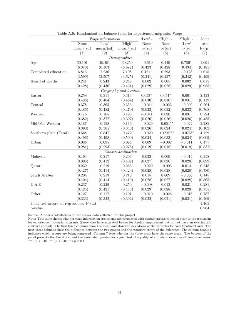
Table A.9: Randomization balance table for experienced migrants: WageWage information ‘Low’ - ‘High’ - ‘High’ - Joint

None ‘Low’ ‘High’ None None ‘Low’ testmean/(sd) mean/(sd) mean/(sd) b/(se) b/(se) b/(se) F/(p)

(1) (2) (3) (4) (5) (6) (7)Demographics

Age 30.101 29.491 30.250 −0.610 0.149 0.759∗ 1.691(6.376) (6.103) (6.672) (0.423) (0.428) (0.434) (0.185)

Completed education 6.815 7.236 7.108 0.421∗ 0.293 −0.128 1.615(3.599) (3.507) (3.625) (0.241) (0.237) (0.242) (0.199)

Heard of deaths 0.241 0.243 0.246 0.002 0.005 0.002 0.015(0.428) (0.430) (0.431) (0.029) (0.028) (0.029) (0.985)

Geography and locationEastern 0.258 0.311 0.313 0.053∗ 0.054∗ 0.001 2.133

(0.438) (0.464) (0.464) (0.030) (0.030) (0.031) (0.119)Central 0.378 0.365 0.356 −0.014 −0.023 −0.009 0.264

(0.486) (0.482) (0.479) (0.033) (0.032) (0.033) (0.768)Western 0.176 0.165 0.196 −0.011 0.020 0.031 0.724

(0.382) (0.372) (0.397) (0.026) (0.026) (0.026) (0.485)Mid/Far Western 0.187 0.158 0.136 −0.029 −0.051∗∗ −0.022 2.285

(0.390) (0.365) (0.343) (0.026) (0.024) (0.024) (0.102)Southern plain (Terai) 0.568 0.547 0.472 −0.020 −0.096∗∗∗ −0.075∗∗ 4.729

(0.496) (0.498) (0.500) (0.034) (0.033) (0.034) (0.009)Urban 0.086 0.095 0.084 0.009 −0.002 −0.011 0.177

(0.281) (0.293) (0.278) (0.019) (0.018) (0.019) (0.837)Chosen destination

Malaysia 0.194 0.217 0.203 0.023 0.009 −0.014 0.358(0.396) (0.412) (0.402) (0.027) (0.026) (0.028) (0.699)

Qatar 0.239 0.219 0.233 −0.020 −0.006 0.014 0.248(0.427) (0.414) (0.423) (0.028) (0.028) (0.028) (0.780)

Saudi Arabia 0.204 0.219 0.213 0.015 0.009 −0.006 0.145(0.404) (0.414) (0.410) (0.028) (0.027) (0.028) (0.865)

U.A.E 0.237 0.229 0.250 −0.008 0.013 0.021 0.281(0.425) (0.421) (0.433) (0.029) (0.028) (0.029) (0.755)

Other 0.127 0.117 0.101 −0.010 −0.026 −0.015 0.757(0.333) (0.322) (0.302) (0.022) (0.021) (0.021) (0.469)

Joint test across all regressions: F-stat 1.165p-value 0.264

Source: Author’s calculations on the survey data collected for this projectNote: This table checks whether wage information treatments are correlated with characteristics collected prior to the treatmentfor experienced potential migrants (those who have migrated before for foreign employment but do not have an existing jobcontract abroad). The first three columns show the mean and standard deviations of the variables for each treatment arm. Thenext three columns show the difference between the two groups and the standard errors of the difference. The column headingindicates which groups are being compared. Column 7 tests whether the three arms have the same mean. The bottom of thepanel presents the F-statistic and the associated p-value for a joint test of equality of all outcomes across all treatment arms.∗∗∗ : p < 0.01; ∗∗ : p < 0.05; ∗ : p < 0.1

61

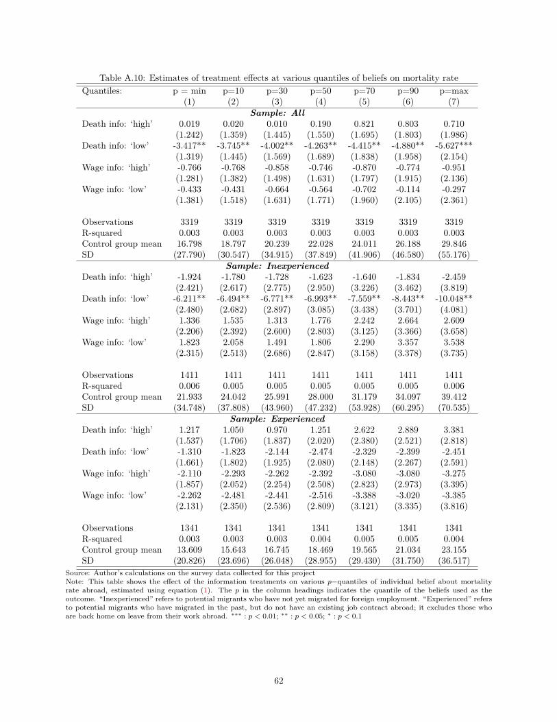
Table A.10: Estimates of treatment effects at various quantiles of beliefs on mortality rateQuantiles: p = min p=10 p=30 p=50 p=70 p=90 p=max

(1) (2) (3) (4) (5) (6) (7)Sample: All

Death info: ‘high’ 0.019 0.020 0.010 0.190 0.821 0.803 0.710(1.242) (1.359) (1.445) (1.550) (1.695) (1.803) (1.986)

Death info: ‘low’ -3.417** -3.745** -4.002** -4.263** -4.415** -4.880** -5.627***(1.319) (1.445) (1.569) (1.689) (1.838) (1.958) (2.154)

Wage info: ‘high’ -0.766 -0.768 -0.858 -0.746 -0.870 -0.774 -0.951(1.281) (1.382) (1.498) (1.631) (1.797) (1.915) (2.136)

Wage info: ‘low’ -0.433 -0.431 -0.664 -0.564 -0.702 -0.114 -0.297(1.381) (1.518) (1.631) (1.771) (1.960) (2.105) (2.361)

Observations 3319 3319 3319 3319 3319 3319 3319R-squared 0.003 0.003 0.003 0.003 0.003 0.003 0.003Control group mean 16.798 18.797 20.239 22.028 24.011 26.188 29.846SD (27.790) (30.547) (34.915) (37.849) (41.906) (46.580) (55.176)

Sample: InexperiencedDeath info: ‘high’ -1.924 -1.780 -1.728 -1.623 -1.640 -1.834 -2.459

(2.421) (2.617) (2.775) (2.950) (3.226) (3.462) (3.819)Death info: ‘low’ -6.211** -6.494** -6.771** -6.993** -7.559** -8.443** -10.048**

(2.480) (2.682) (2.897) (3.085) (3.438) (3.701) (4.081)Wage info: ‘high’ 1.336 1.535 1.313 1.776 2.242 2.664 2.609

(2.206) (2.392) (2.600) (2.803) (3.125) (3.366) (3.658)Wage info: ‘low’ 1.823 2.058 1.491 1.806 2.290 3.357 3.538

(2.315) (2.513) (2.686) (2.847) (3.158) (3.378) (3.735)

Observations 1411 1411 1411 1411 1411 1411 1411R-squared 0.006 0.005 0.005 0.005 0.005 0.005 0.006Control group mean 21.933 24.042 25.991 28.000 31.179 34.097 39.412SD (34.748) (37.808) (43.960) (47.232) (53.928) (60.295) (70.535)

Sample: ExperiencedDeath info: ‘high’ 1.217 1.050 0.970 1.251 2.622 2.889 3.381

(1.537) (1.706) (1.837) (2.020) (2.380) (2.521) (2.818)Death info: ‘low’ -1.310 -1.823 -2.144 -2.474 -2.329 -2.399 -2.451

(1.661) (1.802) (1.925) (2.080) (2.148) (2.267) (2.591)Wage info: ‘high’ -2.110 -2.293 -2.262 -2.392 -3.080 -3.080 -3.275

(1.857) (2.052) (2.254) (2.508) (2.823) (2.973) (3.395)Wage info: ‘low’ -2.262 -2.481 -2.441 -2.516 -3.388 -3.020 -3.385

(2.131) (2.350) (2.536) (2.809) (3.121) (3.335) (3.816)

Observations 1341 1341 1341 1341 1341 1341 1341R-squared 0.003 0.003 0.003 0.004 0.005 0.005 0.004Control group mean 13.609 15.643 16.745 18.469 19.565 21.034 23.155SD (20.826) (23.696) (26.048) (28.955) (29.430) (31.750) (36.517)

Source: Author’s calculations on the survey data collected for this projectNote: This table shows the effect of the information treatments on various p−quantiles of individual belief about mortalityrate abroad, estimated using equation (1). The p in the column headings indicates the quantile of the beliefs used as theoutcome. “Inexperienced” refers to potential migrants who have not yet migrated for foreign employment. “Experienced” refersto potential migrants who have migrated in the past, but do not have an existing job contract abroad; it excludes those whoare back home on leave from their work abroad. ∗∗∗ : p < 0.01; ∗∗ : p < 0.05; ∗ : p < 0.1

62

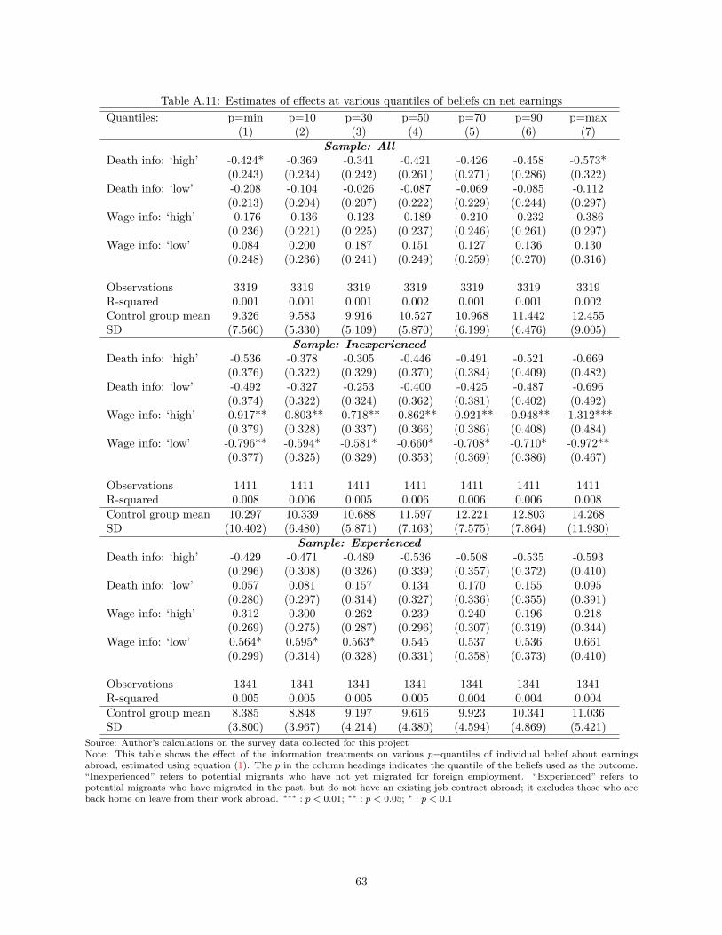
Table A.11: Estimates of effects at various quantiles of beliefs on net earningsQuantiles: p=min p=10 p=30 p=50 p=70 p=90 p=max

(1) (2) (3) (4) (5) (6) (7)Sample: All

Death info: ‘high’ -0.424* -0.369 -0.341 -0.421 -0.426 -0.458 -0.573*(0.243) (0.234) (0.242) (0.261) (0.271) (0.286) (0.322)

Death info: ‘low’ -0.208 -0.104 -0.026 -0.087 -0.069 -0.085 -0.112(0.213) (0.204) (0.207) (0.222) (0.229) (0.244) (0.297)

Wage info: ‘high’ -0.176 -0.136 -0.123 -0.189 -0.210 -0.232 -0.386(0.236) (0.221) (0.225) (0.237) (0.246) (0.261) (0.297)

Wage info: ‘low’ 0.084 0.200 0.187 0.151 0.127 0.136 0.130(0.248) (0.236) (0.241) (0.249) (0.259) (0.270) (0.316)

Observations 3319 3319 3319 3319 3319 3319 3319R-squared 0.001 0.001 0.001 0.002 0.001 0.001 0.002Control group mean 9.326 9.583 9.916 10.527 10.968 11.442 12.455SD (7.560) (5.330) (5.109) (5.870) (6.199) (6.476) (9.005)

Sample: InexperiencedDeath info: ‘high’ -0.536 -0.378 -0.305 -0.446 -0.491 -0.521 -0.669

(0.376) (0.322) (0.329) (0.370) (0.384) (0.409) (0.482)Death info: ‘low’ -0.492 -0.327 -0.253 -0.400 -0.425 -0.487 -0.696

(0.374) (0.322) (0.324) (0.362) (0.381) (0.402) (0.492)Wage info: ‘high’ -0.917** -0.803** -0.718** -0.862** -0.921** -0.948** -1.312***

(0.379) (0.328) (0.337) (0.366) (0.386) (0.408) (0.484)Wage info: ‘low’ -0.796** -0.594* -0.581* -0.660* -0.708* -0.710* -0.972**

(0.377) (0.325) (0.329) (0.353) (0.369) (0.386) (0.467)

Observations 1411 1411 1411 1411 1411 1411 1411R-squared 0.008 0.006 0.005 0.006 0.006 0.006 0.008Control group mean 10.297 10.339 10.688 11.597 12.221 12.803 14.268SD (10.402) (6.480) (5.871) (7.163) (7.575) (7.864) (11.930)

Sample: ExperiencedDeath info: ‘high’ -0.429 -0.471 -0.489 -0.536 -0.508 -0.535 -0.593

(0.296) (0.308) (0.326) (0.339) (0.357) (0.372) (0.410)Death info: ‘low’ 0.057 0.081 0.157 0.134 0.170 0.155 0.095

(0.280) (0.297) (0.314) (0.327) (0.336) (0.355) (0.391)Wage info: ‘high’ 0.312 0.300 0.262 0.239 0.240 0.196 0.218

(0.269) (0.275) (0.287) (0.296) (0.307) (0.319) (0.344)Wage info: ‘low’ 0.564* 0.595* 0.563* 0.545 0.537 0.536 0.661

(0.299) (0.314) (0.328) (0.331) (0.358) (0.373) (0.410)

Observations 1341 1341 1341 1341 1341 1341 1341R-squared 0.005 0.005 0.005 0.005 0.004 0.004 0.004Control group mean 8.385 8.848 9.197 9.616 9.923 10.341 11.036SD (3.800) (3.967) (4.214) (4.380) (4.594) (4.869) (5.421)

Source: Author’s calculations on the survey data collected for this projectNote: This table shows the effect of the information treatments on various p−quantiles of individual belief about earningsabroad, estimated using equation (1). The p in the column headings indicates the quantile of the beliefs used as the outcome.“Inexperienced” refers to potential migrants who have not yet migrated for foreign employment. “Experienced” refers topotential migrants who have migrated in the past, but do not have an existing job contract abroad; it excludes those who areback home on leave from their work abroad. ∗∗∗ : p < 0.01; ∗∗ : p < 0.05; ∗ : p < 0.1

63

TableA.12:

Cha

racterist

icsof

theattrite

rsAll

Inexpe

rien

ced

Exp

erienc

edAttrit

ionmeasure

FM

WF

MW

FM

W(1)

(2)

(3)

(4)

(5)

(6)

(7)

(8)

(9)

Dem

ographics

Age

0.417

0.797**

1.005

0.080

0.343

0.756

-0.535

-0.413

0.296

(0.351)

(0.380)

(0.825)

(0.434)

(0.490)

(1.015)

(0.502)

(0.543)

(1.007)

Com

pleted

years

-1.158***

-1.128***

-1.670***

-1.313***

-1.297***

-1.836***

-1.161***

-1.061***

-1.811***

ofscho

oling

(0.178)

(0.188)

(0.344)

(0.271)

(0.291)

(0.508)

(0.301)

(0.315)

(0.555)

Geography

andlocatio

nEa

stern

-0.004

-0.003

0.056

-0.013

0.005

0.143**

-0.005

-0.006

0.073

(0.021)

(0.023)

(0.046)

(0.032)

(0.035)

(0.072)

(0.036)

(0.038)

(0.074)

Central

0.019

0.009

0.061

-0.020

-0.038

-0.031

0.065*

0.053

0.044

(0.023)

(0.025

)(0.048)

(0.037)

(0.040)

(0.072)

(0.039)

(0.041)

(0.075)

Western

-0.038**

-0.030*

-0.079***

-0.014

-0.023

-0.010

-0.072***

-0.062**

-0.092**

(0.016)

(0.018

)(0.027)

(0.018)

(0.019)

(0.036)

(0.026)

(0.029)

(0.045)

Mid/F

arWestern

0.023

0.024

-0.037

0.047

0.057

-0.103*

0.012

0.016

-0.026

(0.019)

(0.021)

(0.035)

(0.034)

(0.038)

(0.056)

(0.030)

(0.032)

(0.053)

Southe

rnPlain

0.035

0.045*

0.129***

-0.020

0.021

0.160**

0.101***

0.082**

0.136*

(Terai)

(0.024)

(0.025)

(0.047)

(0.037)

(0.041)

(0.071)

(0.039)

(0.041)

(0.073)

Urban

0.000

0.007

0.000

-0.007

-0.002

-0.009

0.022

0.028

0.027

(0.013)

(0.014)

(0.027)

(0.019)

(0.021)

(0.036)

(0.024)

(0.026)

(0.049)

Expected

timeof

migratio

nW

ithin

2mon

ths

0.109***

0.131***

0.058

0.068**

0.062*

0.033

0.098**

0.112***

0.111

(0.024)

(0.025)

(0.049)

(0.033)

(0.036)

(0.065)

(0.039)

(0.042)

(0.077)

Certainly

in3

0.113***

0.135***

0.064

0.066**

0.062*

0.029

0.102***

0.114***

0.126

mon

ths

(0.024)

(0.025)

(0.048)

(0.032)

(0.036)

(0.063)

(0.039)

(0.042)

(0.077)

Source:Autho

r’scalculations

onthesurvey

data

collected

forthis

project

Note:

Thistabletestswhether

attritersarediffe

rent

from

non-attriterson

thecharacteristicsshow

nin

theleft

side

ofthetable.

The

measure

ofattritionbe

ingtested

isindicatedby

itscorrespo

ndingletter

inthesecond

row

ofthetablehead

ings.The

measuresof

attritionaredefin

edin

Table4.

Eachcellisasepa

rate

regression

.The

estimated

regression

isyi

=α

+βATTRITi+ε i

whereyiarethecharacteristicsrepo

rted

intheleftmostcolumnan

dATTRITiisthemeasure

ofattritionindicatedby

thecolumnhead

ing

(secon

drow

ofthetable).The

first

row

ofthetablehead

ings

indicate

thesampleforwhich

thetested

isbe

ingpe

rformed.“Inexp

erienced”refers

topo

tentialmigrantswho

have

notyetmigratedforforeignem

ploy

ment.

“Exp

erienced”refers

topo

tentialm

igrantswho

have

migratedin

thepa

st,b

utdo

notha

vean

existing

jobcontract

abroad

;it

exclud

esthosewho

areba

ckho

meon

leavefrom

theirworkab

road

.Coefficients

(β)arerepo

rted

alon

gwithrobu

ststan

dard

errors

inpa

rentheses.

∗∗∗

:p<

0.01

;∗∗:p

<0.

05;

∗:p

<0.

1

64

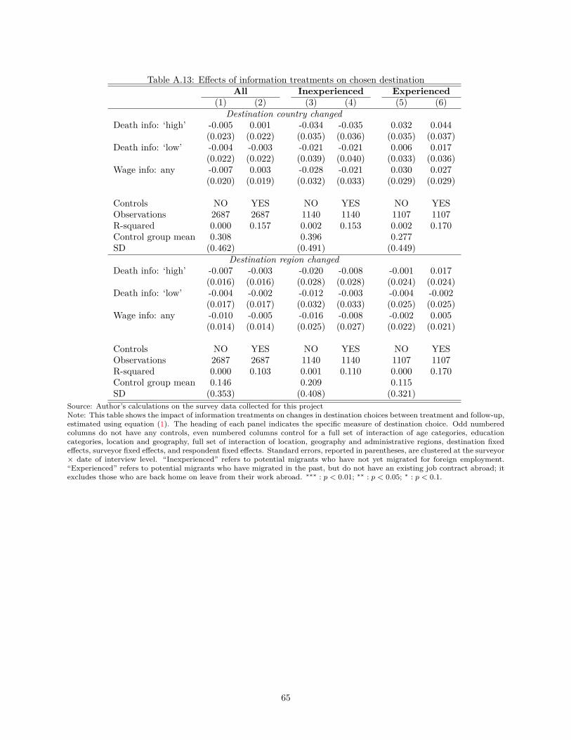
Table A.13: Effects of information treatments on chosen destinationAll Inexperienced Experienced

(1) (2) (3) (4) (5) (6)Destination country changed

Death info: ‘high’ -0.005 0.001 -0.034 -0.035 0.032 0.044(0.023) (0.022) (0.035) (0.036) (0.035) (0.037)

Death info: ‘low’ -0.004 -0.003 -0.021 -0.021 0.006 0.017(0.022) (0.022) (0.039) (0.040) (0.033) (0.036)

Wage info: any -0.007 0.003 -0.028 -0.021 0.030 0.027(0.020) (0.019) (0.032) (0.033) (0.029) (0.029)

Controls NO YES NO YES NO YESObservations 2687 2687 1140 1140 1107 1107R-squared 0.000 0.157 0.002 0.153 0.002 0.170Control group mean 0.308 0.396 0.277SD (0.462) (0.491) (0.449)

Destination region changedDeath info: ‘high’ -0.007 -0.003 -0.020 -0.008 -0.001 0.017

(0.016) (0.016) (0.028) (0.028) (0.024) (0.024)Death info: ‘low’ -0.004 -0.002 -0.012 -0.003 -0.004 -0.002

(0.017) (0.017) (0.032) (0.033) (0.025) (0.025)Wage info: any -0.010 -0.005 -0.016 -0.008 -0.002 0.005

(0.014) (0.014) (0.025) (0.027) (0.022) (0.021)

Controls NO YES NO YES NO YESObservations 2687 2687 1140 1140 1107 1107R-squared 0.000 0.103 0.001 0.110 0.000 0.170Control group mean 0.146 0.209 0.115SD (0.353) (0.408) (0.321)

Source: Author’s calculations on the survey data collected for this projectNote: This table shows the impact of information treatments on changes in destination choices between treatment and follow-up,estimated using equation (1). The heading of each panel indicates the specific measure of destination choice. Odd numberedcolumns do not have any controls, even numbered columns control for a full set of interaction of age categories, educationcategories, location and geography, full set of interaction of location, geography and administrative regions, destination fixedeffects, surveyor fixed effects, and respondent fixed effects. Standard errors, reported in parentheses, are clustered at the surveyor× date of interview level. “Inexperienced” refers to potential migrants who have not yet migrated for foreign employment.“Experienced” refers to potential migrants who have migrated in the past, but do not have an existing job contract abroad; itexcludes those who are back home on leave from their work abroad. ∗∗∗ : p < 0.01; ∗∗ : p < 0.05; ∗ : p < 0.1.

65

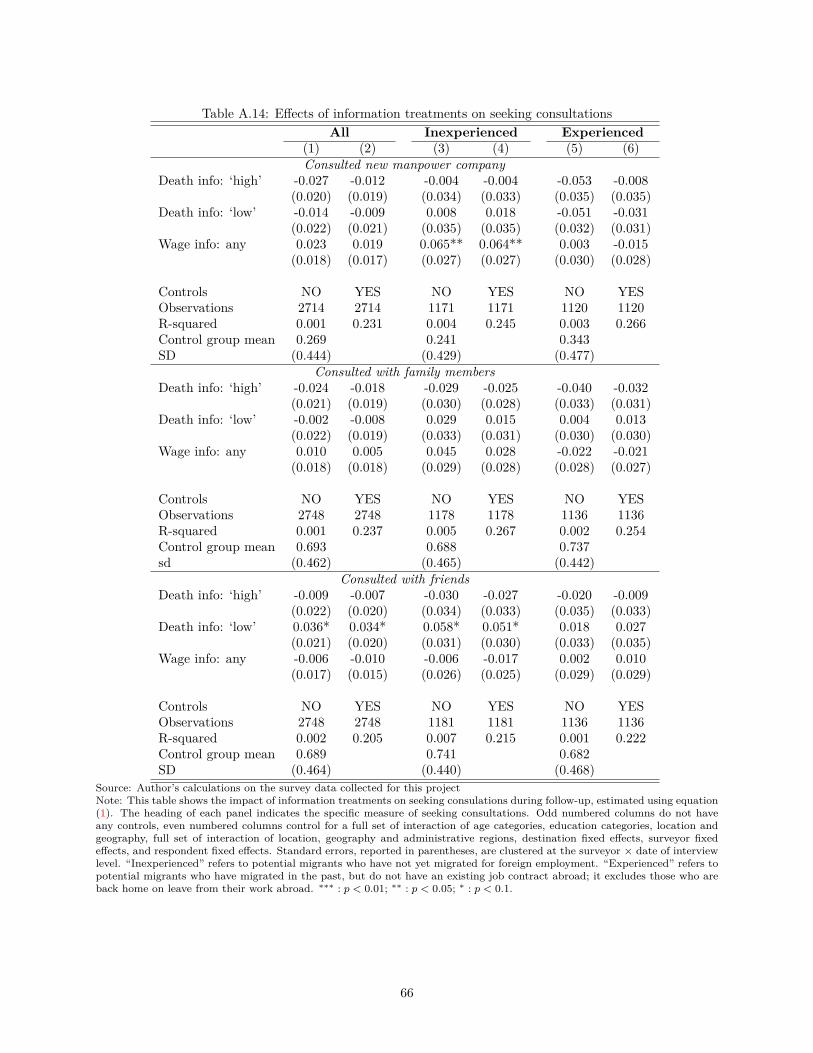
Table A.14: Effects of information treatments on seeking consultationsAll Inexperienced Experienced

(1) (2) (3) (4) (5) (6)Consulted new manpower company

Death info: ‘high’ -0.027 -0.012 -0.004 -0.004 -0.053 -0.008(0.020) (0.019) (0.034) (0.033) (0.035) (0.035)

Death info: ‘low’ -0.014 -0.009 0.008 0.018 -0.051 -0.031(0.022) (0.021) (0.035) (0.035) (0.032) (0.031)

Wage info: any 0.023 0.019 0.065** 0.064** 0.003 -0.015(0.018) (0.017) (0.027) (0.027) (0.030) (0.028)

Controls NO YES NO YES NO YESObservations 2714 2714 1171 1171 1120 1120R-squared 0.001 0.231 0.004 0.245 0.003 0.266Control group mean 0.269 0.241 0.343SD (0.444) (0.429) (0.477)

Consulted with family membersDeath info: ‘high’ -0.024 -0.018 -0.029 -0.025 -0.040 -0.032

(0.021) (0.019) (0.030) (0.028) (0.033) (0.031)Death info: ‘low’ -0.002 -0.008 0.029 0.015 0.004 0.013

(0.022) (0.019) (0.033) (0.031) (0.030) (0.030)Wage info: any 0.010 0.005 0.045 0.028 -0.022 -0.021

(0.018) (0.018) (0.029) (0.028) (0.028) (0.027)

Controls NO YES NO YES NO YESObservations 2748 2748 1178 1178 1136 1136R-squared 0.001 0.237 0.005 0.267 0.002 0.254Control group mean 0.693 0.688 0.737sd (0.462) (0.465) (0.442)

Consulted with friendsDeath info: ‘high’ -0.009 -0.007 -0.030 -0.027 -0.020 -0.009

(0.022) (0.020) (0.034) (0.033) (0.035) (0.033)Death info: ‘low’ 0.036* 0.034* 0.058* 0.051* 0.018 0.027

(0.021) (0.020) (0.031) (0.030) (0.033) (0.035)Wage info: any -0.006 -0.010 -0.006 -0.017 0.002 0.010

(0.017) (0.015) (0.026) (0.025) (0.029) (0.029)

Controls NO YES NO YES NO YESObservations 2748 2748 1181 1181 1136 1136R-squared 0.002 0.205 0.007 0.215 0.001 0.222Control group mean 0.689 0.741 0.682SD (0.464) (0.440) (0.468)

Source: Author’s calculations on the survey data collected for this projectNote: This table shows the impact of information treatments on seeking consulations during follow-up, estimated using equation(1). The heading of each panel indicates the specific measure of seeking consultations. Odd numbered columns do not haveany controls, even numbered columns control for a full set of interaction of age categories, education categories, location andgeography, full set of interaction of location, geography and administrative regions, destination fixed effects, surveyor fixedeffects, and respondent fixed effects. Standard errors, reported in parentheses, are clustered at the surveyor × date of interviewlevel. “Inexperienced” refers to potential migrants who have not yet migrated for foreign employment. “Experienced” refers topotential migrants who have migrated in the past, but do not have an existing job contract abroad; it excludes those who areback home on leave from their work abroad. ∗∗∗ : p < 0.01; ∗∗ : p < 0.05; ∗ : p < 0.1.

66

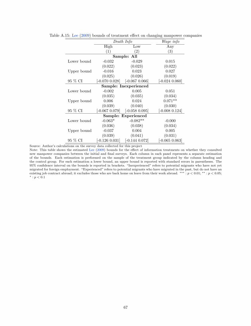
Table A.15: Lee (2009) bounds of treatment effect on changing manpower companiesDeath Info Wage info

High Low Any(1) (2) (3)

Sample: AllLower bound -0.032 -0.029 0.015

(0.022) (0.023) (0.022)Upper bound -0.016 0.023 0.027

(0.025) (0.026) (0.019)95 % CI [-0.070 0.028] [-0.067 0.066] [-0.024 0.060]

Sample: InexperiencedLower bound -0.002 0.005 0.051

(0.035) (0.035) (0.034)Upper bound 0.006 0.024 0.071**

(0.039) (0.040) (0.030)95 % CI [-0.067 0.079] [-0.058 0.095] [-0.008 0.124]

Sample: ExperiencedLower bound -0.063* -0.082** -0.000

(0.036) (0.038) (0.034)Upper bound -0.037 0.004 0.005

(0.039) (0.041) (0.031)95 % CI [-0.126 0.031] [-0.144 0.072] [-0.065 0.063]

Source: Author’s calculations on the survey data collected for this projectNote: This table shows the estimated Lee (2009) bounds for the effect of information treatments on whether they consultednew manpower companies between the initial and final surveys. Each column in each panel represents a separate estimationof the bounds. Each estimation is performed on the sample of the treatment group indicated by the column heading andthe control group. For each estimation a lower bound, an upper bound is reported with standard errors in parentheses. The95% confidence interval on the bounds is reported in brackets. “Inexperienced” refers to potential migrants who have not yetmigrated for foreign employment. “Experienced” refers to potential migrants who have migrated in the past, but do not have anexisting job contract abroad; it excludes those who are back home on leave from their work abroad. ∗∗∗ : p < 0.01; ∗∗ : p < 0.05;∗ : p < 0.1

67

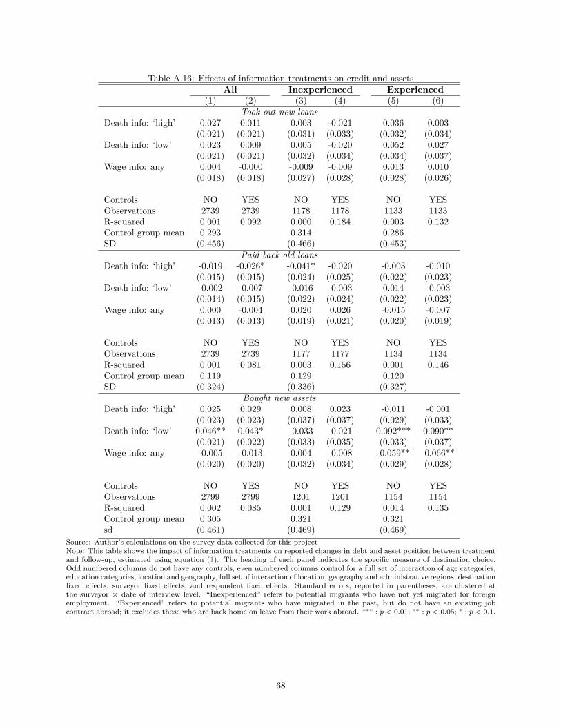
Table A.16: Effects of information treatments on credit and assetsAll Inexperienced Experienced

(1) (2) (3) (4) (5) (6)Took out new loans

Death info: ‘high’ 0.027 0.011 0.003 -0.021 0.036 0.003(0.021) (0.021) (0.031) (0.033) (0.032) (0.034)

Death info: ‘low’ 0.023 0.009 0.005 -0.020 0.052 0.027(0.021) (0.021) (0.032) (0.034) (0.034) (0.037)

Wage info: any 0.004 -0.000 -0.009 -0.009 0.013 0.010(0.018) (0.018) (0.027) (0.028) (0.028) (0.026)

Controls NO YES NO YES NO YESObservations 2739 2739 1178 1178 1133 1133R-squared 0.001 0.092 0.000 0.184 0.003 0.132Control group mean 0.293 0.314 0.286SD (0.456) (0.466) (0.453)

Paid back old loansDeath info: ‘high’ -0.019 -0.026* -0.041* -0.020 -0.003 -0.010

(0.015) (0.015) (0.024) (0.025) (0.022) (0.023)Death info: ‘low’ -0.002 -0.007 -0.016 -0.003 0.014 -0.003

(0.014) (0.015) (0.022) (0.024) (0.022) (0.023)Wage info: any 0.000 -0.004 0.020 0.026 -0.015 -0.007

(0.013) (0.013) (0.019) (0.021) (0.020) (0.019)

Controls NO YES NO YES NO YESObservations 2739 2739 1177 1177 1134 1134R-squared 0.001 0.081 0.003 0.156 0.001 0.146Control group mean 0.119 0.129 0.120SD (0.324) (0.336) (0.327)

Bought new assetsDeath info: ‘high’ 0.025 0.029 0.008 0.023 -0.011 -0.001

(0.023) (0.023) (0.037) (0.037) (0.029) (0.033)Death info: ‘low’ 0.046** 0.043* -0.033 -0.021 0.092*** 0.090**

(0.021) (0.022) (0.033) (0.035) (0.033) (0.037)Wage info: any -0.005 -0.013 0.004 -0.008 -0.059** -0.066**

(0.020) (0.020) (0.032) (0.034) (0.029) (0.028)

Controls NO YES NO YES NO YESObservations 2799 2799 1201 1201 1154 1154R-squared 0.002 0.085 0.001 0.129 0.014 0.135Control group mean 0.305 0.321 0.321sd (0.461) (0.469) (0.469)

Source: Author’s calculations on the survey data collected for this projectNote: This table shows the impact of information treatments on reported changes in debt and asset position between treatmentand follow-up, estimated using equation (1). The heading of each panel indicates the specific measure of destination choice.Odd numbered columns do not have any controls, even numbered columns control for a full set of interaction of age categories,education categories, location and geography, full set of interaction of location, geography and administrative regions, destinationfixed effects, surveyor fixed effects, and respondent fixed effects. Standard errors, reported in parentheses, are clustered atthe surveyor × date of interview level. “Inexperienced” refers to potential migrants who have not yet migrated for foreignemployment. “Experienced” refers to potential migrants who have migrated in the past, but do not have an existing jobcontract abroad; it excludes those who are back home on leave from their work abroad. ∗∗∗ : p < 0.01; ∗∗ : p < 0.05; ∗ : p < 0.1.

68

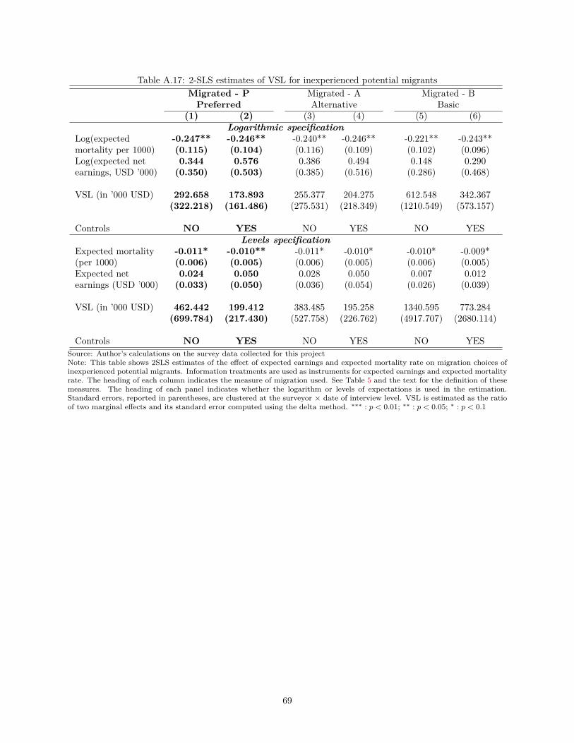
Table A.17: 2-SLS estimates of VSL for inexperienced potential migrantsMigrated - P Migrated - A Migrated - BPreferred Alternative Basic

(1) (2) (3) (4) (5) (6)Logarithmic specification

Log(expected -0.247** -0.246** -0.240** -0.246** -0.221** -0.243**mortality per 1000) (0.115) (0.104) (0.116) (0.109) (0.102) (0.096)Log(expected net 0.344 0.576 0.386 0.494 0.148 0.290earnings, USD ’000) (0.350) (0.503) (0.385) (0.516) (0.286) (0.468)

VSL (in ’000 USD) 292.658 173.893 255.377 204.275 612.548 342.367(322.218) (161.486) (275.531) (218.349) (1210.549) (573.157)

Controls NO YES NO YES NO YESLevels specification

Expected mortality -0.011* -0.010** -0.011* -0.010* -0.010* -0.009*(per 1000) (0.006) (0.005) (0.006) (0.005) (0.006) (0.005)Expected net 0.024 0.050 0.028 0.050 0.007 0.012earnings (USD ’000) (0.033) (0.050) (0.036) (0.054) (0.026) (0.039)

VSL (in ’000 USD) 462.442 199.412 383.485 195.258 1340.595 773.284(699.784) (217.430) (527.758) (226.762) (4917.707) (2680.114)

Controls NO YES NO YES NO YESSource: Author’s calculations on the survey data collected for this projectNote: This table shows 2SLS estimates of the effect of expected earnings and expected mortality rate on migration choices ofinexperienced potential migrants. Information treatments are used as instruments for expected earnings and expected mortalityrate. The heading of each column indicates the measure of migration used. See Table 5 and the text for the definition of thesemeasures. The heading of each panel indicates whether the logarithm or levels of expectations is used in the estimation.Standard errors, reported in parentheses, are clustered at the surveyor × date of interview level. VSL is estimated as the ratioof two marginal effects and its standard error computed using the delta method. ∗∗∗ : p < 0.01; ∗∗ : p < 0.05; ∗ : p < 0.1

69

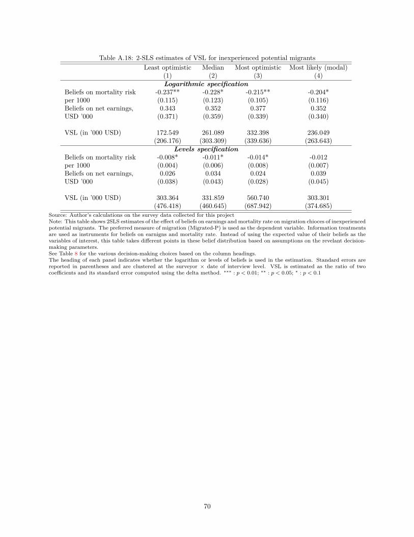
Table A.18: 2-SLS estimates of VSL for inexperienced potential migrantsLeast optimistic Median Most optimistic Most likely (modal)

(1) (2) (3) (4)Logarithmic specification

Beliefs on mortality risk -0.237** -0.228* -0.215** -0.204*per 1000 (0.115) (0.123) (0.105) (0.116)Beliefs on net earnings, 0.343 0.352 0.377 0.352USD ’000 (0.371) (0.359) (0.339) (0.340)

VSL (in ’000 USD) 172.549 261.089 332.398 236.049(206.176) (303.309) (339.636) (263.643)

Levels specificationBeliefs on mortality risk -0.008* -0.011* -0.014* -0.012per 1000 (0.004) (0.006) (0.008) (0.007)Beliefs on net earnings, 0.026 0.034 0.024 0.039USD ’000 (0.038) (0.043) (0.028) (0.045)

VSL (in ’000 USD) 303.364 331.859 560.740 303.301(476.418) (460.645) (687.942) (374.685)

Source: Author’s calculations on the survey data collected for this projectNote: This table shows 2SLS estimates of the effect of beliefs on earnings and mortality rate on migration chioces of inexperiencedpotential migrants. The preferred measure of migration (Migrated-P) is used as the dependent variable. Information treatmentsare used as instruments for beliefs on earnigns and mortality rate. Instead of using the expected value of their beliefs as thevariables of interest, this table takes different points in these belief distribution based on assumptions on the revelant decision-making parameters.See Table 8 for the various decision-making choices based on the column headings.The heading of each panel indicates whether the logarithm or levels of beliefs is used in the estimation. Standard errors arereported in parentheses and are clustered at the surveyor × date of interview level. VSL is estimated as the ratio of twocoefficients and its standard error computed using the delta method. ∗∗∗ : p < 0.01; ∗∗ : p < 0.05; ∗ : p < 0.1

70

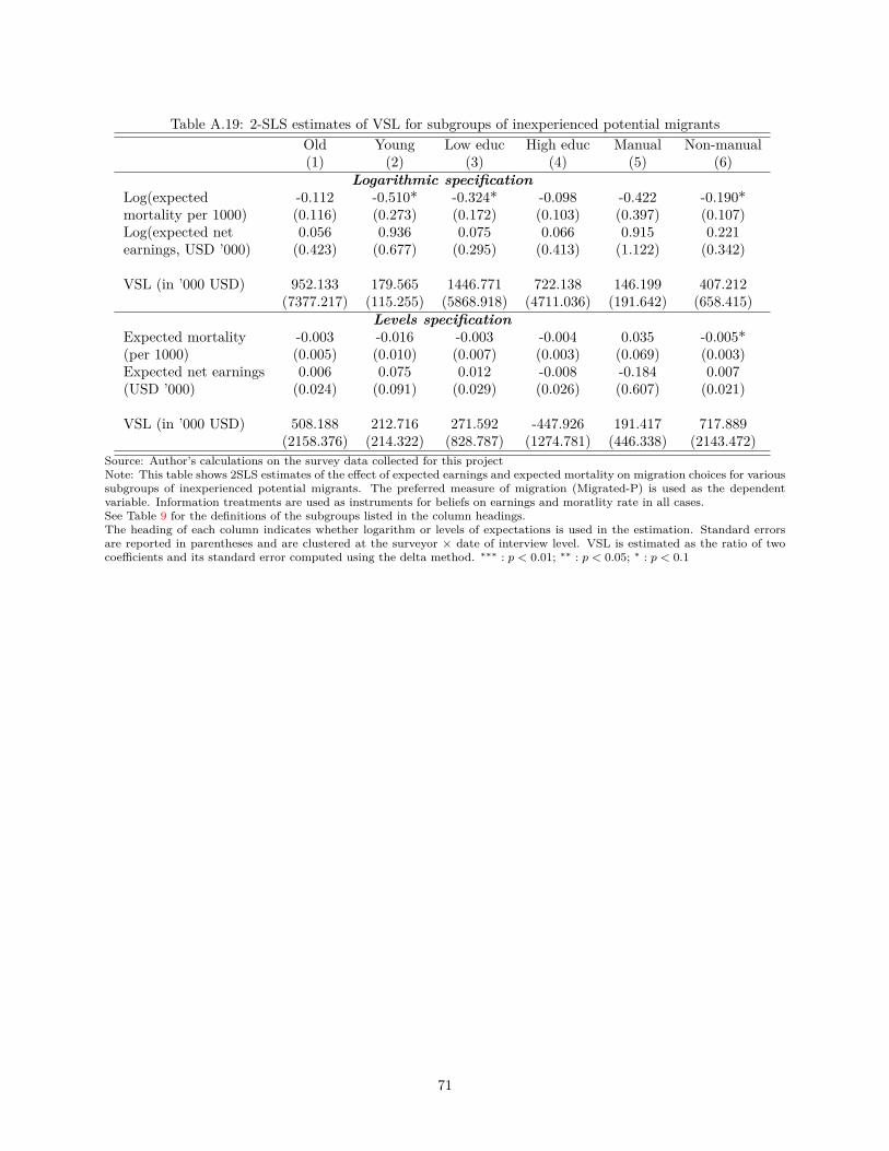
Table A.19: 2-SLS estimates of VSL for subgroups of inexperienced potential migrantsOld Young Low educ High educ Manual Non-manual(1) (2) (3) (4) (5) (6)

Logarithmic specificationLog(expected -0.112 -0.510* -0.324* -0.098 -0.422 -0.190*mortality per 1000) (0.116) (0.273) (0.172) (0.103) (0.397) (0.107)Log(expected net 0.056 0.936 0.075 0.066 0.915 0.221earnings, USD ’000) (0.423) (0.677) (0.295) (0.413) (1.122) (0.342)

VSL (in ’000 USD) 952.133 179.565 1446.771 722.138 146.199 407.212(7377.217) (115.255) (5868.918) (4711.036) (191.642) (658.415)

Levels specificationExpected mortality -0.003 -0.016 -0.003 -0.004 0.035 -0.005*(per 1000) (0.005) (0.010) (0.007) (0.003) (0.069) (0.003)Expected net earnings 0.006 0.075 0.012 -0.008 -0.184 0.007(USD ’000) (0.024) (0.091) (0.029) (0.026) (0.607) (0.021)

VSL (in ’000 USD) 508.188 212.716 271.592 -447.926 191.417 717.889(2158.376) (214.322) (828.787) (1274.781) (446.338) (2143.472)

Source: Author’s calculations on the survey data collected for this projectNote: This table shows 2SLS estimates of the effect of expected earnings and expected mortality on migration choices for varioussubgroups of inexperienced potential migrants. The preferred measure of migration (Migrated-P) is used as the dependentvariable. Information treatments are used as instruments for beliefs on earnings and moratlity rate in all cases.See Table 9 for the definitions of the subgroups listed in the column headings.The heading of each column indicates whether logarithm or levels of expectations is used in the estimation. Standard errorsare reported in parentheses and are clustered at the surveyor × date of interview level. VSL is estimated as the ratio of twocoefficients and its standard error computed using the delta method. ∗∗∗ : p < 0.01; ∗∗ : p < 0.05; ∗ : p < 0.1

71

Appendix B Normal learning from information

Individuals have normally distributed priors over earnings (or mortality risks) with mean θ0 and varianceσ2θ . That is, priors θ ∼ N

(θ0, σ

2θ

). Individuals assume that the signal, s, they see is a random draw from the

distribution N(θ, σ2

s

). Upon receiving the signal, individuals update their prior according to Bayes’ rule.

Normality of the priors and the signals mean that the posterior is also normally distributed with mean andvariance given by

θ|s ∼ N(θ1, σ

2θ1

)= N

(σ2s · θ0 + σ2

θ · sσ2s + σ2

θ

,σ2sσ

2θ

σ2s + σ2

θ

)This simple result has the following direct implications for the effect of the signal (assuming s < θ0 withoutloss of generality):

1. Individuals update towards the signal. That is s < θ1 < θ0. The extent of updating depends upon thevariance of prior and the perceived variance of the signal.

2. Posterior is more precise than the prior or the signal. That is, σ2θ1< min

{σ2θ , σ

2s

}3. The effect of the information in each quantile of the individual belief distribution is increasing (in

magnitude) with the quantile. Denote θ1 (p) − θ0 (p) as the effect of the information on the pth

quantile of the individual belief distribution. Then

D (p) ≡ θ1 (p)− θ0 (p) = (θ1 − θ0) + (σθ1 − σθ) Φ−1 (p)

withD′ (p) = 1

φ (z) (σθ1 − σθ) < 0

where Φ (z) and φ (z) denote the standard normal distribution and density functions respectively. Theinequality follows from 2.

These results are investigated systematically in Table 2 and Appendix Table A.10 for updating in responseto a death signal, in Table 3 and Appendix Table A.11 for updating in response to an earnings signal. Theresults are discussed in Section 4.2.

Furthermore, this simple framework is useful to infer how the subjects perceive the noisiness of theinformation provided to them. The distribution of priors is given by the distribution of the beliefs of theaverage person in the control group and the distribution of the posterior is given by the distribution of thebeliefs of the average person in each of the treatment groups. Using these moments from data and updatingrule given above, I can recover the perceived distribution of signals from which the information provided tothem is drawn. This exercise is useful because the exact nature of the information provided to them leftenough room for them to perceive the signal in different ways. For instance, the wage information providedthe earnings but clearly mentioned the year of information was either 2010 or 2013. Similarly, the deathinformation only provided the number of migrant deaths from a district without giving any information onstock of the migrants from the reference district.

Based on their updating behavior of the inexperienced migrants, the implied distribution of the signal is

72

consistent with the information provided to them.43 The ‘high’ wage information provided to them translatedto a signal with a mean of $6,700 and a standard deviation of $1,200. The actual information provided in thistreatment translates to a net earnings of $5,800 in 2013, which is about 0.75 standard deviation of the impliedmean. It could also be that individuals updated the 2013 information to 2015, making it more relevant tothem. The ‘low’ wage information provided to them translated to a signal with a mean of $6,200 and astandard deviation of $1,600. The actual information provided in this treatment translates to a net earningsof $2,900 in 2010. This information is about 2 standard deviations away from the implied mean of thesignal distribution. This suggests that individuals could indeed be re-interpreting the information providedto them to make it relevant to their decision. For instance, when they saw the information provided to themwas of 2010, they factored in how wages could have evolved in the past five years and adjusted their beliefsaccordingly.44 Some respondents assigned to this treatment group even complained during the survey sayingthat information could not have been true or is irrelevant for now. Furthermore, the implied distribution ofsignal seem similar for the ‘high’ and ‘low’ wage treatments indicating that these two treatments affects thebehavior in a similar way.

Similarly, the ‘high’ death information translated to a signal with a mean mortality rate of 15 per 1000with a standard deviation of 8.7, and the ‘low’ death information translated to a signal with a mean mortalityrate of 13 per 1000 with a standard deviation of 4.4. The actual death rates implied by the information were0.9 and 3.7 per 1000 respectively for the ‘low’ and ‘high’ treatments. This discrepancy could simply reflectthe lack of knowledge about the migrant stock abroad or other biases leading to interpreting the signal withan upward bias.

43The same exercise could not be done with the experienced migrants as the information was irrelevant to them. The averageindividual in the treatment group (posterior) did not have a lower variance of his beliefs than the average individual in thecontrol group (prior).

44Between 2010 and 2013, exchange rates in destination countries appreciated relative to Nepali Rupees by about 30 percent,inflation in Nepal increased by about the same amount. Even with these two adjustments the information provided becomessimilar to the one provided in the ‘high’ treatment.

73