geospatial and temporal dynamics of application …mshafiq/files/spatialapp_tmc.pdfgeospatial and...

1

Geospatial and Temporal Dynamics ofApplication Usage in Cellular Data Networks

M. Zubair Shafiq Lusheng Ji Alex X. Liu Jeffrey Pang Jia Wang

F

Abstract—Significant geospatial and temporal correlations, in termsof traffic volume and application access, exist in cellular networkusage as shown in recent studies on cellular network measurement.Such geospatial and temporal correlation patterns provide localoptimization opportunities to cellular network operators for handlingthe explosive growth in the traffic volume observed in recent years.To the best of our knowledge, in this paper, we provide the firstfine-grained joint characterization of the geospatial and temporaldynamics of application usage in a 3G cellular data network. Ouranalysis is based on two simultaneously collected traces from theradio access network (containing location records) and the corenetwork (containing traffic records) of a tier-1 cellular network inthe United States. To better understand the application usage inour data, we first cluster cell locations based on their applicationdistributions and then study the geospatial and temporal dynamics ofapplication usage across different geographical regions. The resultsof our measurement study present cellular network operators withfine-grained insights that can be leveraged to tune network param-eter settings for better network performance and user experience.

Index Terms—Apps; Cellular Networks

1 INTRODUCTIONCellular network operators have globally observed anexplosive increase in the volume of data traffic inrecent years. Cisco has reported that the volume ofglobal cellular data traffic has tripled (year-over-year)for three years in a row, reaching up to 237 petabytesper month in 2010 [2]. This unprecedented increasein the volume of cellular data traffic is attributedto the increase in the subscriber base, improvingnetwork connection speeds, and improving hardwareand software capabilities of modern smartphones. Incontrast to the traditional wired networks, cellularnetwork operators are faced with the constraint of

• The preliminary version of this paper titled “Characterizing GeospatialDynamics of Application Usage in a 3G Cellular Data Network” waspublished in the proceedings of the 31th Annual IEEE Conference onComputer Communications (INFOCOM), Orlando, Florida, 2012.

• Alex X. Liu is the corresponding author of this paper.• M. Zubair Shafiq is with the Department of Computer Sci-

ence, The University of Iowa, Iowa City, IA, USA. Email:[email protected]

• Alex X. Liu is with the Department of Computer Science andEngineering, Michigan State University, East Lansing, MI, USA.Email:[email protected]

• Lusheng Ji, Jeffrey Pang, and Jia Wang are with AT&TLabs – Research, Bedminster, NJ, USA. Email:{lji, jeffpang, ji-awang}@research.att.com

limited radio frequency spectrum at their disposal.As the communication technologies evolve beyond 3Gto long term evolution (LTE), the competition for thelimited radio frequency spectrum is becoming evenmore intense. Therefore, cellular network operatorsincreasingly focus on optimizing different aspects ofthe network by customized design and managementto improve key performance indicators (KPIs).

There are three aspects of a cellular network thatpresent significant optimization potential to the net-work operators: (1) diverse application mix constitutingthe data traffic, (2) variations in the traffic depending uponthe geo-location of users, and (3) temporal variations inthe traffic. It has been shown that the performanceof different applications constituting the data trafficin cellular networks is sensitive to various networkKPIs [11], [16]. Tso et al. also showed that the networkperformance perceived by users is strongly relatedto their geolocation and mobility patterns [25]. Fur-thermore, Xu et al. showed that different applicationshave different temporal dynamics [29]. Combiningthe aforementioned aspects, cellular network oper-ators can potentially find even better opportunitiesfor network optimization. However, to the best ofour knowledge, no prior work has jointly studiedthe relationship between application usage, temporaldynamics, and users’ geospatial movement patterns.

Trestian et al. conducted a study that provided thefirst evidence of geographic correlation of users’ “in-terests” in a cellular network [24]. They showed thatusers in different geographical regions have differ-ent interests; for example, people mostly access mailURLs from office locations and access more musicURLs from residential locations. However, cellularnetwork operators not only need to know that there isgeographic correlation of interests, but also how thoseinterests translate into different types of applicationtraffic. This is because it is the type of traffic (bursty,bulk transfers, streaming, etc.) that determines howan operator can best optimize each geographic area.Furthermore, cellular network operators would liketo be able to map the aforementioned coarse-grainedgeographic correlation to a more fine-grained cellsector correlation, as this is typically the smallest unit

2

that operators can configure. Paul et al. separatelystudied application usage and geospatial patterns ofaggregate traffic volume; however, they did not studycorrelation between them [16]. Other prior studies thateither study application usage or geospatial patterns(but not both simultaneously) include but are notlimited to [6], [11], [15], [22], [25], [27]. Further detailsof prior art are in Section 8.

To the best of our knowledge, this paper presentsthe first fine-grained joint characterization of thegeospatial and temporal dynamics of application us-age in a 3G cellular data network. We summarize thekey contributions of our research as follows:

1) Methodology: For our study, we collected twotraces from the cellular network: (1) periodicallycollected cell sector records of devices from theradio network and (2) data traffic records of IPflows passing through the core network. Due tothe massive size of the collected traces, our dataset is limited to 32 hours worth of data in De-cember 2010 covering a large metropolitan areaspanning more than 1, 200 km2 in the UnitedStates.We study application usage characteristics ofusers across more than two thousand 3G celllocations. For the systematic analysis of appli-cation usage across these cell locations, we firstcluster cells based on their application distribu-tion. The results of our clustering experimentsshow that cells can be robustly categorized intoa small number of clusters using traffic volumein terms of byte, packet, flow, and unique usercount distributions. Using the clustering results,we analyze the geospatial patterns of applicationusage across different geographical regions, e.g.downtown, university, and suburban areas. Toextract geospatial dependence patterns, we uti-lize basic cluster composition analysis, intensityfunction analysis, and point-pattern based co-location analysis in this paper. To study the tem-poral dynamics of geospatial dependencies inapplication usage, we apply the aforementionedgeospatial analysis techniques on the updatedcell clustering results for different time intervalssuch as 0000hrs-0300hrs, 0300hrs-0600hrs.

2) Findings and Implications: The results of ourgeospatial and temporal analysis experimentsreveal new insights that have important implica-tions for network optimization. A major findingof our measurement study is that cell clusteringresults are significantly different for traffic vol-ume in terms of byte, packet, flow count, andunique user count distributions across differentgeographical regions. These results present op-erators with an opportunity to fine-tune net-work parameter settings for different applica-tions. However, they also suggest that opera-

GGSN

SGSN

SGSN

RNC

RNC

RNCNode Bs

Node Bs

Node Bs

Internet

Other

External

Networks

UEs

UEs

UEs

Radio link

Radio Access Network Core Network

Gi

Gi

Gn

GnRadio link

Radio link

Fig. 1. 3G UMTS cellular data network.

tors should not optimize cells solely by traf-fic volume in terms of byte, packet, or flowcounts because this may negatively impact theperformance of other low volume–but popular–applications. Furthermore, we find that there isdifferentiation between the application mix ofdifferent cells even within a close region such as auniversity, downtown, or suburb. Consequently,there are opportunities for fine-grained networkoptimization within close regions. Finally, wefind that cell locations with particular appli-cation mixes have tendency to be co-located.This information can be used by operators tooptimize frequency planning and managementof transmission power and handovers in co-located cells.

2 BACKGROUND AND DATAIn this section, we first provide a brief overviewof 3G Universal Mobile Telecommunications System(UMTS) cellular data network architecture and thenprovide information about the data set used in ourstudy.

2.1 Network ArchitectureFigure 1 shows the architecture of a typical 3G UMTScellular data network. A UMTS cellular data networkconsists of two separate networks: radio access net-work and a core network. The network elements inthese networks are logically connected to each other ina tree topology. The following list orders the elementsfrom the leaves to the root of the tree: user equipment(UE), cell sectors, NodeBs, Radio Network Controllers(RNCs), Serving General Packet Radio Service [GPRS]Support Nodes (SGSNs), and Gateway GPRS SupportNodes (GGSNs). A UE, or cellular device, connects toone or more cell sectors in the radio access network.Each sector is distinguished by a different antennaon a NodeB, or a physical base station. The datatraffic generated by a cellular device is first sent toa NodeB and then to a RNC, which manages radioaccess network control signalling such as transmissionscheduling and handovers. Each RNC typically sendsand receives traffic to/from several NodeBs that coverhundreds of cell sectors, each of which in turn servesmany users in its coverage area. The core networkconsists of SGSNs facing cellular devices and GGSNsthat connect to external networks. RNCs send datatraffic to SGSNs, which then send it to GGSNs. Finally,

3

GGSNs send data traffic to external networks, suchas the Internet. In order to support mobility withoutdisrupting a cellular device’s IP network connections,the IP address of the device is anchored at the GGSN.The IP address association is formed when the deviceconnects to the network and establishes a Packet DataProtocol (PDP) Context that facilitates tunnelling ofIP traffic from the device to the GGSN. These tun-nels, implemented using the GPRS Tunneling Protocol(GTP), carry IP packets between the cellular devicesand their peering GGSNs.

2.2 Data SetsIn this paper, we use two anonymized data sets froma tier-1 cellular network operator for our study. Thefirst data set contains flow-level information of IPtraffic carried in PDP Context tunnels (i.e., all datatraffic sent to and from cellular devices). This dataset is collected from all the links between SGSNs andGGSNs, called Gn links, in the core network and cov-ers a 3% random sample of devices. The data containsthe following information for each IP flow per minute:start and end timestamps, per-flow traffic volume interms of bytes and packets, device identifiers, useridentifiers, and application identifiers. All device anduser identifiers (e.g., IMEI, IMSI) are anonymized toprotect privacy without affecting the usefulness of ouranalysis. The data set does not permit the reversalof the anonymization or re-identification of users.For proprietary reasons, the results presented in thispaper are sum-normalized. However, normalizationdoes not change the range of the metrics used in thisstudy. Furthermore, the missing information due tonormalization does not affect the understanding ofour analysis.

Application identifiers include information aboutapplication protocol (e.g., HTTP, DNS, SIP), class (e.g.,streaming video, web, email), and, in the case ofapplications registered in popular “App Stores,” theunique name of the application. Applications areidentified using a combination of port information,HTTP host and user-agent information, and otherheuristics [5]. Since we encounter tens of thousandsof applications in the data, we only examine thetop 100 by traffic volume. These top applicationscomprise the vast majority of all data traffic (morethan 95% of all data traffic in terms of byte volume),so understanding the remainder is not critical for thepurpose of traffic engineering [29]. Furthermore, wecategorize applications into the following applicationrealms, in no particular order, based on their func-tionality and traffic type (streaming, interactive, etc.)[21]. (1) ads, (2) mixed HTTP streaming, (3) appstore, (4) media optimization, (5) dating, (6)email, (7) games, (8) news info image media, (9)maps, (10) misc, (11) mms, (12) music audio, (13)p2p, (14) radio audio, (15) social network, (16)streaming video, (17) voip, (18) vpn, (19) web

browsing/other http. For example, mixed HTTPstreaming includes apps like YouTube, radioaudio includes apps like TuneIn Radio, socialnetwork includes apps like Facebook, and musicaudio includes apps like Pandora. Note that theapplication realms are non-overlapping. Applicationscan belong to multiple categories because of their dualfunctionality and traffic type. For example, YouTubecan be classified as mixed HTTP streaming orstreaming video; however, we classify YouTubeas mixed HTTP streaming because it mainly usesHTTP streaming on smartphones [19].

Although this data set also contains the cell loca-tions associated with each PDP context, these loca-tions are often inaccurate because they are typicallyonly recorded when PDP contexts are established andmay not be updated for hours or days even whenusers are mobile [28]. Therefore, we cannot studyfine-grained geospatial dynamics of application usageusing the location information collected only from thecore network. To get accurate location information, wecollect a second data set at RNCs in the radio accessnetwork. The second data set contains fine-grainedlogs of signaling events at the RNCs, which includehandover events. By joining the PDP sessions in thefirst data set with complete handover information inthe second data set based on their timestamps, we getaccurate cell locations at a 2 second granularity for IPflows in the first data set. In practice, a device may beconnected to multiple cell sectors at the same time toallow transmission of uplink data from HSPA devicesto the most suitable sector based on factors such assignal strength, load, interference, etc. For the pur-poses of our study, we use the primary or serving cell,which is the sector that actually transmits downlinkdata to HSPA devices [20]. It is important to note thatthe second data set cannot be continuously collectedover long durations of time because its collectioncan introduce non-trivial additional overheads at theRNCs. For this study, we simultaneously collectedboth data sets over a weekday period of 32 hours from1600hrs on December 6, 2010 till 2400hrs December7, 2010.

The data sets cover a large metropolitan area span-ning more than 1, 200 km2 in the United States. Themetropolitan area had complete 3G coverage; there-fore, it would be rare for a device to handoff toany neighboring 2.5G cells. Thus, the data sets covermore than two thousand 3G cells in the metropolitanarea, but do not cover any 2.5G cells. It accountsfor hundreds of gigabytes of IP traffic, consisting ofhundreds of millions of packets and tens of millionsof flows, and covers tens of thousands of devices. Al-though we cannot study long-term application usagepatterns due to the significant overheads of collectingthe second data set over longer timescales, we believeour results still provide generalizable insights due tothe volume of data and number of devices studied.

4

3 AGGREGATE MEASUREMENT ANALYSISIn this section, we explain the details of our measure-ment analysis conducted on the two data sets col-lected from the cellular networks to study the geospa-tial dynamics of application usage. Towards this end,we start by examining the temporal dynamics ofaggregate traffic, and then study application usagedistributions in the traffic, and finally investigate therelative popularity of individual applications acrossdifferent cell locations.

3.1 Temporal AnalysisAs mentioned in Section 2, all traffic records in ourdata set are timestamped and are tagged with appli-cation and cell identifiers. Below, we analyze hourlyvariations in the traffic volume during 24 hours onDecember 7, 2012 for the sake of clarity. We first studythe temporal dynamics of aggregate traffic volume.Figure 2 shows the temporal dynamics of aggregatetraffic in terms of byte, packet, flow, and user counts.As reported in prior literature [16], [22], [29], weobserve a strong diurnal behavior in aggregate traffic.However, we observe two daily peaks – instead ofa daily peak observed in prior literature [22], [29]– and the second peak is around mid-night, whichmight reflect users’ peculiar activity patterns in themetropolitan area studied in this paper. We notethat the aggregate traffic volume during day timeis significantly more than that during night time.Furthermore, the variations in traffic volume are dif-ferent across bytes, packets, flows, and users. We alsostudy the temporal dynamics of traffic volume fordifferent applications. Figure 3 shows the temporaldynamics of traffic belonging to four applications forbyte, packet, flow, and user counts. As observed foraggregate traffic, we observe strong diurnal charac-teristics in temporal dynamics across all applications.However, there are interesting differences across theseapplications. For instance, we note that traffic volumesof dating and social network applications peakaround late night in terms of byte count. On the otherhand, traffic volume of web browsing and mapsapplications peak around noon and afternoon. We also

1 2 3 4 5 6 7 8 9 10 11 12 13 14 15 16 17 18 19 20 21 22 23 24

0.02

0.03

0.04

0.05

0.06

0.07

Time (Hour)

Pro

babi

lity

Byte Packet Flow User

Fig. 2. Temporal dynamics of aggregate traffic in termsof bytes, packets, flows, and users.

observe subtle differences in the temporal dynamics oftraffic volume for byte, packet, flow, and user counts.We further elaborate on these observations in the restof this section.

3.2 Application Analysis

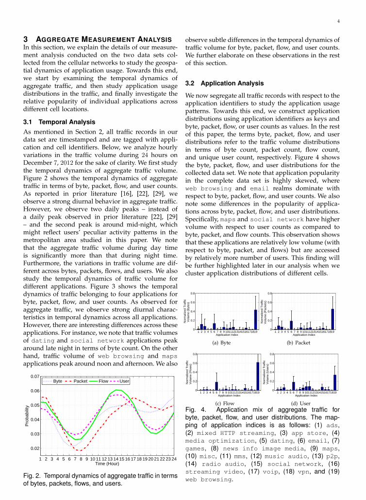
We now segregate all traffic records with respect to theapplication identifiers to study the application usagepatterns. Towards this end, we construct applicationdistributions using application identifiers as keys andbyte, packet, flow, or user counts as values. In the restof this paper, the terms byte, packet, flow, and userdistributions refer to the traffic volume distributionsin terms of byte count, packet count, flow count,and unique user count, respectively. Figure 4 showsthe byte, packet, flow, and user distributions for thecollected data set. We note that application popularityin the complete data set is highly skewed, whereweb browsing and email realms dominate withrespect to byte, packet, flow, and user counts. We alsonote some differences in the popularity of applica-tions across byte, packet, flow, and user distributions.Specifically, maps and social network have highervolume with respect to user counts as compared tobyte, packet, and flow counts. This observation showsthat these applications are relatively low volume (withrespect to byte, packet, and flows) but are accessedby relatively more number of users. This finding willbe further highlighted later in our analysis when wecluster application distributions of different cells.

1 2 3 4 5 6 7 8 9 101112131415161718190

0.2

0.4

0.6

0.8

Application Index

Nor

mal

ized

Tra

ffic

Vol

ume

(Byt

es)

(a) Byte

1 2 3 4 5 6 7 8 9 101112131415161718190

0.2

0.4

0.6

0.8

Application Index

Nor

mal

ized

Tra

ffic

Vol

ume

(Pac

kets

)

(b) Packet

1 2 3 4 5 6 7 8 9 101112131415161718190

0.2

0.4

0.6

0.8

Application Index

Nor

mal

ized

Tra

ffic

Vol

ume

(Flo

ws)

(c) Flow

1 2 3 4 5 6 7 8 9 101112131415161718190

0.2

0.4

0.6

0.8

Application Index

Nor

mal

ized

Tra

ffic

Vol

ume

(Use

rs)

(d) UserFig. 4. Application mix of aggregate traffic forbyte, packet, flow, and user distributions. The map-ping of application indices is as follows: (1) ads,(2) mixed HTTP streaming, (3) app store, (4)media optimization, (5) dating, (6) email, (7)games, (8) news info image media, (9) maps,(10) misc, (11) mms, (12) music audio, (13) p2p,(14) radio audio, (15) social network, (16)streaming video, (17) voip, (18) vpn, and (19)web browsing.

5

1 2 3 4 5 6 7 8 9 10 11 12 13 14 15 16 17 18 19 20 21 22 23 240

0.01

0.02

0.03

0.04

0.05

0.06

0.07

0.08

Time (Hour)

Pro

babi

lity

datingmapssocial networkweb

(a) Byte

1 2 3 4 5 6 7 8 9 10 11 12 13 14 15 16 17 18 19 20 21 22 23 240

0.02

0.04

0.06

0.08

0.1

0.12

Time (Hour)

Pro

babi

lity


(b) Packet

1 2 3 4 5 6 7 8 9 10 11 12 13 14 15 16 17 18 19 20 21 22 23 24

0.02

0.04

0.06

0.08

0.1

Time (Hour)

Pro

babi

lity


(c) Flow

1 2 3 4 5 6 7 8 9 10 11 12 13 14 15 16 17 18 19 20 21 22 23 240

0.02

0.04

0.06

0.08

0.1

Time (Hour)

Pro

babi

lity


(d) User

Fig. 3. Temporal dynamics of applications in terms of bytes, packets, flows, and users.

1% 5% 10% 25% 50%100%0

0.2

0.4

0.6

0.8

1

Cell Index (reverse−sorted w.r.t volume)

CD

F

dating maps social newtork web

(a) Byte

1% 5% 10% 25% 50%100%0

0.2

0.4

0.6

0.8

1


CD

F


(b) Packet

1% 5% 10% 25% 50%100%0

0.2

0.4

0.6

0.8

1


CD

F


(c) Flow

1% 5% 10% 25% 50%100%0

0.2

0.4

0.6

0.8

1


CD

F


(d) User

Fig. 5. Distributions of traffic volume with respect to byte, packet, flow, and user counts across all cell sectorlocations.

3.3 Geospatial Analysis

We now study the relative popularity of a given ap-plication across different cell locations in our data set.Figure 5 shows the cumulative distribution function(CDF) of traffic volume of dating, maps, socialnetwork, and web browsing applications with re-spect to byte, packet, flow, and user counts acrossall cells in our data set. Our first observation is that

applications are not equally popular across all cellsin our data set. Furthermore, the popularity of someapplications is more skewed than others across cells.For instance, all traffic volume of dating applicationis generated from less than 5% of all cells. On the otherhand, web browsing is the most ubiquitous applica-tion realm. However, even for web browsing, 80%of the byte traffic volume is generated from 50% of all

6

cells. It is also interesting to note the differences in thebyte, packet, flow, and user volume of applicationsacross cells. For instance, the distribution of bytevolume of social network is more skewed thanmaps across cells; however, this trend is reversed forflow and user volume distributions. This observationindicates that flows and users in a fraction of cellsdominate byte volume for social network appli-cations.

Until now we have established three major findings:(1) traffic volumes of applications exhibit strong diur-nal characteristics, (2) the popularity of a given appli-cation realm varies across different cell locations, and(3) the traffic volume of a few application realms dom-inate others overall. These findings suggest strongdependence of application usage on geospatial andtemporal dynamics. We follow a three step method-ology to systematically conduct our analysis. First,we group the application usage distributions of cellsusing an unsupervised clustering algorithm. Second,we conduct a comprehensive analysis of geospatialdynamics of application usage across clusters usinggeospatial analysis techniques. Third, we analyze thetemporal dynamics of geospatial dependencies in ap-plication usage. The goal of our analysis is to identifypatterns in our data and to formulate new hypothesesabout the underlying processes that gave rise to thedata. We now separately discuss the aforementionedsteps in the following sections.

4 CELL CLUSTERINGTo study the application usage patterns for any givencell, we now segregate all traffic records with respectto the application and cell identifiers. Our goal isto cluster cells into a manageable number of groupsbased on their application usage distributions. It isimportant to cluster cells by byte, packet, and flowdistributions to understand which sectors have similartraffic distributions. It is also important to understandhow cells cluster by user distributions because theapplications that are used widely but infrequently bymany users will not be well represented relative to thebyte, packet, or flow counts of higher volume appli-cations, even if those applications are not as popular.This argument follows our earlier observation fromFigure 4.

We utilize a well-known unsupervised clusteringalgorithm called k-means to cluster application dis-tributions of cells. The k-means algorithm is a simpleyet effective technique to cluster feature vectors intoa predefined k number of groups [13]. The selectionof appropriate value of k is crucial and is an openresearch problem [4]. Several heuristics have beenproposed in prior literature, which primarily focus onthe change in intra-cluster dissimilarity for increasingvalues of k [8], [12], [14]. A well-known heuristic,called gap statistic, can be used to compare the changein intra-cluster dissimilarity Wk for given data and

that for a reference null distribution [23]. Gap statisticprovides a statistical method to find the elbow ofintra-cluster dissimilarity Wk as the values of k isvaried over B iterations. Gap statistic is defined as:

Gap(k) =1

B

B∑b=1

log(Wkb)− log(Wk),

where Wkb denotes the within-cluster dispersion of areference data set from a uniform distribution overthe range of the observed data. Using gap statistic,the optimal value of k is chosen to be the smallestone for which:

Gap(k) ≥ Gap(k + 1)− σk+1,

where σ denotes the standard deviation of within-cluster dispersions in reference data sets. In this work,we set the value of B = 1000 and the initial centroid israndomly selected in each iteration to avoid any bias.Figure 6 shows the plot of gap statistic for varyingvalues of k for byte distributions. We observe thatGap(4) ≥ Gap(5)− σ5, so we select the optimal valueof k = 4. After selecting the value of k = 4 usinggap statistic, we apply k-means clustering algorithmto cluster application distributions of cells into fourgroups. Similar results were obtained for packet, flow,and user distributions.

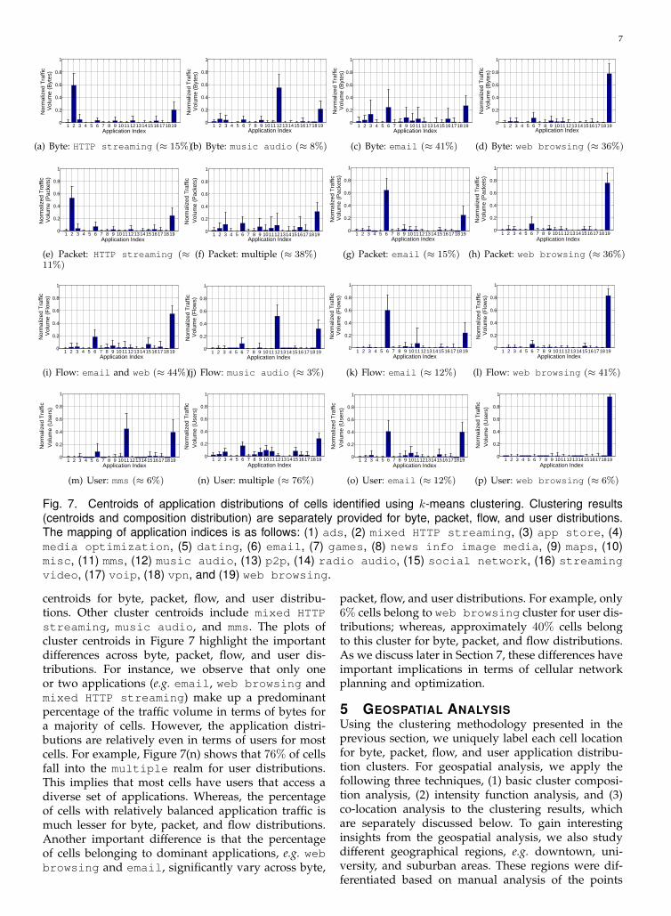
To gain insights into the clustering results, we plotfour cluster centroids of byte, packet, flow, and userdistributions in Figure 7. The error bars represent theintra-cluster standard deviation for each application.While the size of error bars may be affected by thenumber of applications and traffic volume for eachcategory, we observe that traffic volume generallycorrelates with standard deviation rather than thenumber of applications. We label the cluster centroidsusing their popular application types. The clustercentroids that do not have any outright popularapplication are labeled as multiple. In Figure 7,we also provide the percentage distribution of cellsacross all cluster types. As expected, we observe thatweb browsing and email are the common cluster

2 4 6 8 10

5

5.2

5.4

5.6

5.8

6

6.2

6.4

k

Gap

(k)

Fig. 6. Gap statistic for finding the suitable number ofclusters for traffic distributions of cells.

7

1 2 3 4 5 6 7 8 9 101112131415161718190

0.2

0.4

0.6

0.8

1

Application Index

Nor

mal

ized

Tra

ffic

Vol

ume

(Byt

es)

(a) Byte: HTTP streaming (≈ 15%)

1 2 3 4 5 6 7 8 9 101112131415161718190

0.2

0.4

0.6

0.8

1

Application Index

Nor

mal

ized

Tra

ffic

Vol

ume

(Byt

es)

(b) Byte: music audio (≈ 8%)

1 2 3 4 5 6 7 8 9 101112131415161718190

0.2

0.4

0.6

0.8

1

Application Index

Nor

mal

ized

Tra

ffic

Vol

ume

(Byt

es)

(c) Byte: email (≈ 41%)

1 2 3 4 5 6 7 8 9 101112131415161718190

0.2

0.4

0.6

0.8

1

Application Index

Nor

mal

ized

Tra

ffic

Vol

ume

(Byt

es)

(d) Byte: web browsing (≈ 36%)

1 2 3 4 5 6 7 8 9 101112131415161718190

0.2

0.4

0.6

0.8

1

Application Index

Nor

mal

ized

Tra

ffic

Vol

ume

(Pac

kets

)

(e) Packet: HTTP streaming (≈11%)

1 2 3 4 5 6 7 8 9 101112131415161718190

0.2

0.4

0.6

0.8

1

Application Index

Nor

mal

ized

Tra

ffic

Vol

ume

(Pac

kets

)

(f) Packet: multiple (≈ 38%)

1 2 3 4 5 6 7 8 9 101112131415161718190

0.2

0.4

0.6

0.8

1

Application Index

Nor

mal

ized

Tra

ffic

Vol

ume

(Pac

kets

)

(g) Packet: email (≈ 15%)

1 2 3 4 5 6 7 8 9 101112131415161718190

0.2

0.4

0.6

0.8

1

Application Index

Nor

mal

ized

Tra

ffic

Vol

ume

(Pac

kets

)

(h) Packet: web browsing (≈ 36%)

1 2 3 4 5 6 7 8 9 101112131415161718190

0.2

0.4

0.6

0.8

1

Application Index

Nor

mal

ized

Tra

ffic

Vol

ume

(Flo

ws)

(i) Flow: email and web (≈ 44%)

1 2 3 4 5 6 7 8 9 101112131415161718190

0.2

0.4

0.6

0.8

1

Application Index

Nor

mal

ized

Tra

ffic

Vol

ume

(Flo

ws)

(j) Flow: music audio (≈ 3%)

1 2 3 4 5 6 7 8 9 10 11 12 13 14 15 16 17 18 190

0.2

0.4

0.6

0.8

1

Application Index

Nor

mal

ized

Tra

ffic

Vol

ume

(Flo

ws)

(k) Flow: email (≈ 12%)

1 2 3 4 5 6 7 8 9 101112131415161718190

0.2

0.4

0.6

0.8

1

Application Index

Nor

mal

ized

Tra

ffic

Vol

ume

(Flo

ws)

(l) Flow: web browsing (≈ 41%)

1 2 3 4 5 6 7 8 9 101112131415161718190

0.2

0.4

0.6

0.8

1

Application Index

Nor

mal

ized

Tra

ffic

Vol

ume

(Use

rs)

(m) User: mms (≈ 6%)

1 2 3 4 5 6 7 8 9 101112131415161718190

0.2

0.4

0.6

0.8

1

Application Index

Nor

mal

ized

Tra

ffic

Vol

ume

(Use

rs)

(n) User: multiple (≈ 76%)

1 2 3 4 5 6 7 8 9 101112131415161718190

0.2

0.4

0.6

0.8

1

Application Index

Nor

mal

ized

Tra

ffic

Vol

ume

(Use

rs)

(o) User: email (≈ 12%)

1 2 3 4 5 6 7 8 9 101112131415161718190

0.2

0.4

0.6

0.8

1

Application Index

Nor

mal

ized

Tra

ffic

Vol

ume

(Use

rs)

(p) User: web browsing (≈ 6%)

Fig. 7. Centroids of application distributions of cells identified using k-means clustering. Clustering results(centroids and composition distribution) are separately provided for byte, packet, flow, and user distributions.The mapping of application indices is as follows: (1) ads, (2) mixed HTTP streaming, (3) app store, (4)media optimization, (5) dating, (6) email, (7) games, (8) news info image media, (9) maps, (10)misc, (11) mms, (12) music audio, (13) p2p, (14) radio audio, (15) social network, (16) streamingvideo, (17) voip, (18) vpn, and (19) web browsing.

centroids for byte, packet, flow, and user distribu-tions. Other cluster centroids include mixed HTTPstreaming, music audio, and mms. The plots ofcluster centroids in Figure 7 highlight the importantdifferences across byte, packet, flow, and user dis-tributions. For instance, we observe that only oneor two applications (e.g. email, web browsing andmixed HTTP streaming) make up a predominantpercentage of the traffic volume in terms of bytes fora majority of cells. However, the application distri-butions are relatively even in terms of users for mostcells. For example, Figure 7(n) shows that 76% of cellsfall into the multiple realm for user distributions.This implies that most cells have users that access adiverse set of applications. Whereas, the percentageof cells with relatively balanced application traffic ismuch lesser for byte, packet, and flow distributions.Another important difference is that the percentageof cells belonging to dominant applications, e.g. webbrowsing and email, significantly vary across byte,

packet, flow, and user distributions. For example, only6% cells belong to web browsing cluster for user dis-tributions; whereas, approximately 40% cells belongto this cluster for byte, packet, and flow distributions.As we discuss later in Section 7, these differences haveimportant implications in terms of cellular networkplanning and optimization.

5 GEOSPATIAL ANALYSISUsing the clustering methodology presented in theprevious section, we uniquely label each cell locationfor byte, packet, flow, and user application distribu-tion clusters. For geospatial analysis, we apply thefollowing three techniques, (1) basic cluster composi-tion analysis, (2) intensity function analysis, and (3)co-location analysis to the clustering results, whichare separately discussed below. To gain interestinginsights from the geospatial analysis, we also studydifferent geographical regions, e.g. downtown, uni-versity, and suburban areas. These regions were dif-ferentiated based on manual analysis of the points

8

of interest. For example, the region around a univer-sity campus was classified as university, whereas theregions surrounding co-located housing areas wereclassified as suburbs.

5.1 Cluster Composition AnalysisIn the cluster composition analysis, we study thedistribution of cells belonging to different clusters invarious geographical regions. This analysis aims touncover the cases where cells belonging to a particularcluster type are more prevalent in certain geographi-cal regions.

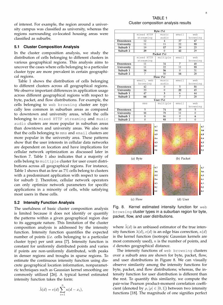
Table 1 shows the distribution of cells belongingto different clusters across all geographical regions.We observe important differences in application usageacross different geographical regions with respect tobyte, packet, and flow distributions. For example, thecells belonging to web browsing cluster are typi-cally less common in suburban areas as comparedto downtown and university areas, while the cellsbelonging to mixed HTTP streaming and musicaudio clusters are more popular in suburban areasthan downtown and university areas. We also notethat the cells belonging to mms and email clusters aremore popular in the university area. These patternsshow that the user interests in cellular data networksare dependent on location and have implications forcellular network optimization as discussed later inSection 7. Table 1 also indicates that a majority ofcells belong to multiple cluster for user count distri-butions across all geographical regions. For instance,Table 1 shows that as few as 7% cells belong to clusterswith a predominant application with respect to usersfor suburb 2. Therefore, cellular network operatorscan only optimize network parameters for specificapplications in a minority of cells, while satisfyingmost users in these cells.

5.2 Intensity Function AnalysisThe usefulness of basic cluster composition analysisis limited because it does not identify or quantifythe patterns within a given geographical region dueto its aggregate nature. This limitation of the clustercomposition analysis is addressed by the intensityfunction. Intensity function quantifies the expectednumber of points (i.e. cells belonging to a particularcluster type) per unit area [7]. Intensity function isconstant for uniformly distributed points and variesif points are non-uniformly distributed, with peaksin denser regions and troughs in sparse regions. Toestimate the continuous intensity function using dis-crete geographical location information, nonparamet-ric techniques such as Gaussian kernel smoothing arecommonly utilized [26]. A typical kernel estimatedintensity function takes the form:

λ̃(d) = e(d)

n∑i=1

κ(d− xi),

TABLE 1Cluster composition analysis results

Byte (%)mixed HTTP music email webstreaming audio browsing

Downtown 12 4 37 47University 11 11 22 55Suburb 1 19 17 39 25Suburb 2 29 0 42 29

Packet (%)mixed HTTP multiple email webstreaming browsing


Flow (%)email, web music email webbrowsing audio browsing


User (%)mms multiple email web

browsingDowntown 5 74 15 5University 11 78 11 0Suburb 1 8 86 0 6Suburb 2 0 93 7 0

(a) Byte (b) Packet

(c) Flow (d) User

Fig. 8. Kernel estimated intensity function for webbrowsing cluster types in a suburban region for byte,packet, flow, and user distributions.

where λ̃(d) is an unbiased estimator of the true inten-sity function λ(d), e(d) is an edge bias correction, κ(d)is the kernel function (isotropic Gaussian kernels aremost commonly used), n is the number of points, andd denotes geographical distance.

The intensity functions of web browsing clustersover a suburb area are shown for byte, packet, flow,and user distributions in Figure 8. We can visuallyobserve similarity among the intensity functions forbyte, packet, and flow distributions; whereas, the in-tensity function for user distribution is different thanthe rest. To quantify this similarity, we compute thepair-wise Pearson product-moment correlation coeffi-cient (denoted by ρ, |ρ| ∈ [0, 1]) between two intensityfunctions [18]. The magnitude of one signifies perfect

9

Fig. 9. Difference between intensity functions of musicaudio clusters and email + web browsing clustersfor byte distribution.

correlation and zero signifies no correlation at allbetween the two given intensity functions. Pearsonproduct-moment correlation coefficient is defined as:

ρλ̃1,λ̃2=E[(λ̃1 − µλ̃1

)(λ̃2 − µλ̃2)]

σλ̃1σλ̃2

,

where E and σ respectively denote the expected valueand standard deviation. As expected from visualobservation, we find that |ρ| ≥ 0.9 for all possi-ble combinations of the intensity functions of byte,packet, and flow clusters; however, |ρ| ≈ 0.6 amongthe intensity functions of user clusters and that ofbyte, packet, or flow clusters. The visual inspection ofintensity functions also shows that even within a closeregion such as a university, downtown, or suburb,there is differentiation between the application mix ofdifferent cells. Consequently there are opportunitiesfor fine-grained network optimization within closeregions, which are discussed later in Section 7. Notethat such detailed analysis is made possible in ourstudy because the mobility information in our data setobtained from radio access network is fine-grained.

We can also identify the geographical areas whereone type of traffic is more prevalent than others usingthe difference of the intensity functions. For suchgeographical areas, cellular network operators canoptimize network parameters for specific performancemetrics. In Figure 9, we add up the intensity functionsof email and web browsing clusters and plot itsdifference to the intensity function of music audio.We observe two distinct geographical areas whereeither email and web browsing or music audiotraffic is dominant. It is well-known that email/webbrowsing and music traffic have conflicting Qualityof Service (QoS) requirements. This type of analysisprovides more actionable insights as compared to thebasic cluster composition analysis described earlier.

5.3 Co-location Analysis

The intensity function is designed for univariategeospatial analysis to identify the geographical re-gions where an application is popular. As we showin Section 5.2, it can also be extended for multivariategeospatial analysis, by utilizing the differences among

individual intensity functions, to identify the geo-graphical regions where an application is more popu-lar than the rest. However, the multivariate intensityfunction analysis does not convey precise informationabout co-location of cells belonging to different clus-ters. Such information is useful to cellular networkoperators for frequency planning and management ofhandovers among co-located cells.

To characterize the co-location characteristics ofcells belonging to different clusters, there are two can-didate point pattern interaction analysis techniques:(1) Ripley’s cross-K function, and (2) nearest neighborfunction [3]. Ripley’s cross-K is a mean based statisticthat is defined as a function of distance between twopoint sets, which represent cluster cell locations forthe present problem. On the other hand, the nearestneighbor function specifically considers the nearestneighbors of one point set from another point set as afunction of distance. Among these two techniques, wechoose the nearest neighbor function because networkoperators are primarily interested in findings aboutimmediately co-located cell locations. To define thenearest neighbor function for two sets of points i andj, let Gij(h) be the probability that the distance froma randomly selected point i to the nearest point j isless then or equal to h. Note that G is a non-symmetricmeasure. Given i and j represent the cell locations oftwo clusters, Figure 10 plots the CDFs of Gij(h) forall byte, packet, flow, and user clusters over a rangeof h. The ordering of G CDFs indicates the relativeattraction between cell locations of different clusters.Specifically, Gij(h) > Gik(h) shows that cell locationsof cluster i are closer to cell locations of cluster j ascompared those of cluster k. We provide the mostsignificant observations for byte, packet, flow, anduser clusters below. For byte clusters, we observe thatmixed HTTP streaming and music audio cellstend to be co-located. For packet clusters, we observethat mixed HTTP streaming and multiple cellstend to be co-located. For flow clusters, we observethat email and music audio cells tend to be co-located. For user clusters, a major observation is thatmms and web browsing cells are mostly co-located.

6 TEMPORAL ANALYSISIn this section, we analyze the temporal dynamics ofgeospatial dependencies in application usage. We sep-arately analyze each of the geospatial analysis tech-niques used in the previous section, including clustercomposition, intensity function, and co-location anal-yses. Recall that these geospatial analysis techniquesoperate on the clustering results obtained in Section4. For temporal analysis of these geospatial analysistechniques, we follow a three step process. First, weseparately construct application distributions of allcells for different time intervals, e.g. 0000hrs-0300hrs,0300hrs-0600hrs, etc. Second, we re-label applicationdistributions of cells with the centroids identified in

10

0 0.01 0.02

0.1

0.2

0.3

0.4

0.5

0.6

0.7

h

CD

F

web browsingmusic audioemail

(a) Byte : mixed HTTPstreaming

0 0.01 0.02

0.1

0.2

0.3

0.4

0.5

0.6

0.7

h

CD

F

HTTP streamingweb browsingemail

(b) Byte: music audio

0 0.01 0.02

0.1

0.2

0.3

0.4

0.5

0.6

0.7

h

CD

F

HTTP streamingweb browsingmusic audio

(c) Byte: email

0 0.01 0.02

0.1

0.2

0.3

0.4

0.5

0.6

0.7

h

CD

F

HTTP streamingmusic audioemail

(d) Byte: web browsing

0 0.01 0.02

0.1

0.2

0.3

0.4

0.5

0.6

0.7

h

CD

F

web browsingemailmultiple

(e) Packet: mixed HTTP stream.

0 0.01 0.02

0.1

0.2

0.3

0.4

0.5

0.6

0.7

h

CD

F

web browsingemailHTTP streaming

(f) Packet: multiple

0 0.01 0.02

0.1

0.2

0.3

0.4

0.5

0.6

0.7

h

CD

F

web browsingHTTP streamingmultiple

(g) Packet: email

0 0.01 0.02

0.1

0.2

0.3

0.4

0.5

0.6

0.7

h

CD

F

emailHTTP streamingmultiple

(h) Packet: web browsing

0 0.01 0.02

0.1

0.2

0.3

0.4

0.5

0.6

0.7

h

CD

F

emailweb browsingmusic audio

(i) Flow: email and web

0 0.01 0.02

0.1

0.2

0.3

0.4

0.5

0.6

0.7

h

CD

F

email and webemailweb browsing

(j) Flow: music audio

0 0.01 0.02

0.1

0.2

0.3

0.4

0.5

0.6

0.7

h

CD

F

email and webweb browsingmusic audio

(k) Flow: email

0 0.01 0.02

0.1

0.2

0.3

0.4

0.5

0.6

0.7

h

CD

F

email and webemailmusic audio

(l) Flow: web browsing

0 0.01 0.02

0.1

0.2

0.3

0.4

0.5

0.6

0.7

h

CD

F

emailmultipleweb browsing

(m) User: mms

0 0.01 0.02

0.1

0.2

0.3

0.4

0.5

0.6

0.7

h

CD

F

mmsemailweb browsing

(n) User: multiple

0 0.01 0.02

0.1

0.2

0.3

0.4

0.5

0.6

0.7

h

CD

F

mmsmultipleweb browsing

(o) User: email

0 0.01 0.02

0.1

0.2

0.3

0.4

0.5

0.6

0.7

h

CD

F

mmsemailmultiple

(p) User: web browsing

Fig. 10. Nearest neighbor metric for co-location analysis.

Section 4. Finally, using the new labels, we recomputeand analyze results for the three geospatial analysistechniques. Next we separately present the temporalanalysis for all of them.

6.1 Cluster Composition AnalysisThe cluster composition results of the byte distri-bution for different time intervals and geographicalregions are provided in Figure 11. Overall, we ob-serve some fluctuations in the cluster compositionresults for different time intervals. For instance, indowntown region, the percentage of cells belong-ing to web browsing cluster is more than emailcluster for 0600hrs-0900hrs, 0900hrs-1200hrs, 1200hrs-1500hrs, 1500hrs-1800hrs, and 1800hrs-2100hrs timeintervals. However, this trend is reversed for 0000hrs-0300hrs, 0300hrs-0600hrs, and 2100hrs-2400hrs timeintervals. Moreover, mixed HTTP streaming ac-counts for more traffic in suburbs as compared to

university area. We observe several of these variationsacross applications and geographical regions. Theseobservations indicate that cellular network operatorsshould take into account such temporal variationswhile deploying pre-dominant application specificnetwork optimization strategies.

6.2 Intensity Function Analysis

Figure 12 plots kernel estimated intensity functionof web browsing cluster for different time inter-vals in a suburban region. Similar to the temporalvariations observed in cluster composition analysisresults, we observe some fluctuations in the shapeof intensity function plots. We can identify threemajor high intensity regions at top-right, middle, andbottom-left of the plots. These regions have varyingrelative intensities at different time intervals withsome distinct patterns. For example, the middle region

11

(a) 0000hrs–0300hrs (b) 0300hrs–0600hrs (c) 0600hrs–0900hrs (d) 0900hrs–1200hrs

(e) 1200hrs–1500hrs (f) 1500hrs–1800hrs (g) 1800hrs–2100hrs (h) 2100hrs–2400hrs

Fig. 12. Temporal dynamics of kernel estimated intensity function for web browsing byte distribution clustersin a suburban region.

Per

cent

age

0000–0300 0300–0600 0600–0900 0900–1200 1200–1500 1500–1800 1800–2100 2100–24000

20

40

60

80

100mixed HTTP streaming music audio email web browsing

(a) Downtown

Per

cent

age

0000–0300 0300–0600 0600–0900 0900–1200 1200–1500 1500–1800 1800–2100 2100–24000

20

40

60

80


(b) University

Per

cent

age

0000–0300 0300–0600 0600–0900 0900–1200 1200–1500 1500–1800 1800–2100 2100–24000

20

40

60

80


(c) Suburb 1

Per

cent

age

0000–0300 0300–0600 0600–0900 0900–1200 1200–1500 1500–1800 1800–2100 2100–24000

20

40

60

80


(d) Suburb 2

Fig. 11. Temporal dynamics of cluster compositionanalysis results for byte distributions.

has the highest intensity for 0900hrs-1200hrs, 1200hrs-1500hrs, and 1500hrs-1800hrs time intervals. Thus,fine-grained tuning of network parameters shouldincorporate temporal variations.

0 0.01 0.020.2

0.3

0.4

0.5

0.6

0.7

h

CD

F

0000hrs−0300hrs0300hrs−0600hrs0600hrs−0900hrs0900hrs−1200hrs1200hrs−1500hrs1500hrs−1800hrs1800hrs−2100hrs2100hrs−2400hrs

Fig. 13. Temporal dynamics of nearest neighbor met-ric for co-location between mixed HTTP streamingand music audio byte distribution clusters.

6.3 Co-location AnalysisFigure 13 plots the CDFs of Gij(h) for mixedHTTP streaming and music audio byte distribu-tion clusters in different time intervals. Similar to thecluster composition and intensity function analysesresults, we observe a pattern in co-location mixedHTTP streaming and music audio clusters. Theordering of CDFs in Figure 13 shows that the prob-ability of their co-location is higher during 0300hrs-1800hrs and it drops substantially for other timeintervals. Cellular network operators should take intoaccount such temporal variations for network plan-ning and management among neighboring cells.

7 MAJOR FINDINGS AND IMPLICATIONSIn this section, we first provide a summary of majorfindings of our study and then provide an example ofhow operators can leverage the findings for networkoptimization.

7.1 Summary of Findings1) A few application realms dominate others in our data

set (Figure 4). We observed that web browsingand email are overall the most popular appli-cations in our data set. This observation presents

12

an optimization opportunity for cellular opera-tors specifically for these applications.

2) Any given application does not enjoy the same levelof popularity across different cell locations (Figure5). This finding implies that cellular networkoperators cannot take “one size fits all” approachin optimizing network parameters for specificapplications.

3) Application usage has diurnal characteristics (Fig-ure 3). We observed that web browsing andmaps applications have peak usage around noonand afternoon. On the other hand, dating andsocial network applications have peak us-age around late night. Consequently, cellularnetwork operators need to dynamically adaptvarious network parameters for optimal perfor-mance.

4) Application mix significantly varies across differentcell sectors (Table 1). From cluster compositionanalysis, we observed that application mixessignificantly vary across downtown, university,and suburban regions. Furthermore, applicationmix of two same type of regions (e.g. suburb 1and suburb 2) show significant similarity. There-fore, cellular network operators can generalizetheir optimization strategies across regions ofthe same type to some extent. In addition, wealso observed that music and video applica-tions are popular in a fraction of cells acrossall regions. In contrast to web browsing andemail traffic, these applications are streamingin nature. Therefore, cellular network operatorscan again fine-tune radio network parametersettings for them.

5) The popularity of different applications significantlyvaries even within a given region (Figures 8 and 9).For more detailed optimization strategies, cellu-lar network operators can utilize the differenceof the intensity function of two applications toidentify distinct cell locations where either ofthe applications dominant. Given the knowl-edge of the application preferences for a specificcell location, the cellular network operator mayfine tune the QoS profile settings and the RNCadmission control procedure when processingRadio Access Bearer (RAB) assignment requestsfor that specific cell.

6) Certain applications have a higher probability ofco-location (Figure 10). Network operators canuse this co-location information for frequencyplanning and handover management amongco-located cells. For instance, cells with morestreaming traffic should handover users to theneighboring cells quicker compared to the cellswith mostly best effort traffic like email.

7) Geospatial dependencies also have temporal varia-tions (Figures 11, 12, and 13). Cellular networkoperators need to dynamically optimize network

parameters and settings as discussed in abovefindings.

8) Application distributions significantly vary for byte,packet, flow, and user counts (Figure 4 and Ta-ble 1). This finding implies that cellular net-work operators may not optimize cells solely bybyte, packet, or flow volume as this may neg-atively impact other low volume–yet popular–applications that many users use in those cells.As a result, there is only a small set of cellswhere a specific application is popular withrespect to all of the byte, packet, flow, and usercounts. This leaves cellular network operatorswith a minority of cells where operators can op-timize for specific applications while satisfyingmost users.

7.2 ImplicationsCellular network operators can leverage the afore-mentioned findings to optimize various network pa-rameters to improve performance. Below, we showusing trace-driven simulations that cellular networkoperators can adapt Radio Resource Control (RRC)state machine inactivity timers to improve perfor-mance [1]. UEs acquire and release radio resourcesby transitioning to different states in their RRC statemachines, which are synchronously maintained by theUEs and network. Figure 14(a) shows the RRC statemachine with three states: Idle, Forward Access Chan-nel (FACH), and Dedicated Channel (DCH) – eachwith progressively more allocated radio resources.When a UE has some data to transfer, it is promotedto a higher energy state. Likewise, a UE is demotedto a lower energy state based on inactivity timeouts.Shorter inactivity timeouts result in more efficientradio resource utilization via more frequent state pro-motions. However, frequent state promotions can alsoresult in degraded user experience especially for delaysensitive applications such as web browsing. There-fore, RRC inactivity timers can be increased in webbrowsing cell sectors to improve user experience. Onthe other hand, RRC inactivity timers can be reducedin cell sectors belonging to delay tolerant applicationclusters such as music audio for more efficient ra-dio resource utilization. The RRC state machine ofevery user is simulated using the RNC logs whilefocusing on the DCH state, which has the highestallocated radio resources compared to all RRC states.We study the effect of varying DCH→FACH RRCtimeout parameter (denoted by TDCH→FACH) on radioresource utilization efficiency for music audio cellsectors and state promotion delay for web browsingcell sectors in Figures 14(b) and 14(c). In Figure 14(b),we observe that idle DCH occupation time decreasesin music audio cell sectors for decreasing values ofTDCH→FACH. Due to the buffer-based streaming natureof traffic in music audio cell sectors, cellular net-work operators can reduce the values of RRC inactiv-

13

(a) RRC State Machine

100

101

102

0

0.2

0.4

0.6

0.8

1

Idle DCH Occupation/User (seconds)

CD

F

2610

(b) Idle DCH state occupation time in musicaudio cell sectors for varying TDCH→FACH

100

101

102

0

0.2

0.4

0.6

0.8

1

Promotion Delay/User (seconds)

CD

F

2610

(c) State promotion delay in web browsingcell sectors for varying TDCH→FACH

Fig. 14. Effect of tuning DCH→FACH timeout parameter (TDCH→FACH) on performance metrics.

ity timeouts to free up radio channels to accommodateadditional users without affecting user experience. InFigure 14(c), we observe that state promotion delayincreases in web browsing cell sectors for decreas-ing values of TDCH→FACH. Therefore, cellular networkoperators can increase the values of RRC inactivitytimeouts to reduce the delays and improve users’ webbrowsing experience.

Although the findings and implications presentedhere are based on traffic traces collected 3 years agofrom a 3G cellular network, we argue they wouldtranslate to current 4G LTE networks. For instance,the findings about geospatial and temporal dynamicsof application usage are not specific to a particularradio access technology. Moreover, LTE networks useRRC state machines similar to 3G networks and aresubject to similar performance tradeoffs based on RRCparameters [10]. For example, the promotion delay isreported to be 260ms (compared to 2 seconds in 3G)and the inactivity timer is reported to be 12 seconds(compared to 12 seconds in 3G) in an operational LTEnetwork [9], [17]. 4G LTE cellular network operatorscan tune these parameters to optimize performancefor different applications in various cell sectors.

8 RELATED WORKSeveral studies have examined cellular network datatraffic, but do not study the relationship between ap-plication usage and location as we do in this paper [6],[11], [15], [16], [22], [24], [27], [29]. The seminal workthat provided first evidence of geographic correlationof users’ interests in a cellular network is by Trestianet al. in [24]. The authors categorized web requestsinto six groups: mail, social networking, trading, mu-sic, news, and dating; and categorized locations into‘home’ and ‘work’. Their study focused on differencesin users’ interests across different locations. Later, Xuet al. also provided evidence of variation in app usageacross different US states [29]. There are two majorlimitations of these studies that we overcame in thispaper. First, they only examined web requests (HTTPURLs) or smartphone apps, but traffic in moderncellular networks can be differentiated with respect toapplication protocol (e.g., HTTP, DNS, SIP) and class

(e.g., streaming audio, streaming video, web, email).On the other hand, our data set is more representativeof mobile data usage as we identify and analyze 19application realms in all IP traffic, not only in HTTPURLs as in [24] or app name as in [29]. Second,they showed differentiation in application interestsat the macro-scale but not at the micro-scale (cellsectors), this leaves the open question how granulargeospatial differentiation actually is. On the otherhand, cell sector locations in our traces are accurate toa finer timescales because they are collected directlyfrom a UMTS radio network, not from core networkservers, which do not record all cell changes due tohandovers [28]. This accuracy enables us to detectdistinct differences in application usage among cellsectors very close to each other.

9 CONCLUSION

In this paper, we jointly characterized the geospatialand temporal dynamics of application usage in a 3Gcellular data network. Using traces collected from thenetwork of a tier-1 cellular operator in the UnitedStates, we first clustered cell locations based on theirapplication usage and then conducted the geospatialand temporal analysis of cells belonging to differentclusters. The results of our empirical study revealedthat the cell clustering results are significantly dif-ferent for byte, packet, flow, and user distributionsacross different geographical regions. However, ourresults also suggested that care should be exercisedso that cells are not optimized solely with respect totraffic volume based on byte, packet, or flow countsbecause this may negatively impact other low volumeapplications used by most users in those cells. Theseand other findings of our measurement analysis haveimportant implications in terms of network designand optimization. To our best knowledge, this pa-per presents the first attempt to conduct fine-grainedanalysis of the geospatial and temporal dynamics ofapplication usage in cellular networks.

Potential extensions of this work include analyz-ing geospatial and temporal dynamics of applicationusage in cellular data networks using: (1) multipledata sets collected from the same location at different

14

times, (2) multiple data sets collected from differentlocations at the same time, and (3) data sets col-lected over a long time duration. The key challengein obtaining these traces is that data collection atthe RNCs introduces non-trivial overheads, whichcan jeopardize network operation particularly duringpeak hours.

REFERENCES

[1] Radio Resource Control (RRC) Protocol specification. Techni-cal Report TS 25.331, 3GPP.

[2] Cisco Visual Networking Index: Global Mobile Data TrafficForecast Update, 2010-2015. White Paper, February 2011.

[3] R. S. Bivand, E. J. Pebesma, and V. Gomez-Rubio. AppliedSpatial Data Analysis with R. Springer, 2008.

[4] M. M.-T. Chiang and B. Mirkin. Experiments for the numberof clusters in k-means. In Lecture Notes in Computer Science,Progress in Artificial Intelligence, 2007.

[5] J. Erman, A. Gerber, M. T. Hajiaghayi, D. Pei, andO. Spatscheck. Network-aware forward caching. In WWW,2009.

[6] H. Falaki, R. Mahajan, S. Kandula, D. Lymberopoulos,R. Govindan, and D. Estrin. Diversity in smartphone usage.In ACM MobiSys, 2010.

[7] R. Haining. Spatial Data Analysis: Theory and Practice. Cam-bridge University Press, 2003.

[8] J. Hartigan. Clustering Algorithms. J. Wiley & Sons, 1975.[9] J. Huang, F. Qian, A. Gerber, Z. M. Mao, S. Sen, and

O. Spatscheck. A Close Examination of Performance andPower Characteristics of 4G LTE Networks. In ACM MobiSys,2012.

[10] J. Huang, F. Qian, Y. Guo, Y. Zhou, Q. Xu, Z. M. Mao, S. Sen,and O. Spatscheck. An In-depth Study of LTE: Effect ofNetwork Protocol and Application Behavior on Performance.In ACM SIGCOMM, 2013.

[11] J. Huang, Q. Xu, B. Tiwana, Z. M. Mao, M. Zhang, andV. Bahl. Anatomizing application performance differences onsmartphones. In ACM MobiSys, 2010.

[12] A. Jain and R. Dubes. Algorithms for Clustering Data. PrenticeHall, 1988.

[13] J. MacQueen. Some methods for classification and analysis ofmultivariate observations. In Fifth Berkeley Symposium on MathStatistics and Probability, 1967.

[14] B. Mirkin. Clustering for Data Mining: A Data Recovery Approach.Chapman and Hall, 2005.

[15] B. M. Orstad and E. Reizer. End-to-end key performance indi-cators in cellular networks. Master’s thesis, Agder UniversityCollege, Norway, 2006.

[16] U. Paul, A. P. Subramanian, M. M. Buddhikot, and S. R. Das.Understanding traffic dynamics in cellular data networks. InIEEE Infocom, 2011.

[17] F. Qian, Z. Wang, A. Gerber, Z. M. Mao, S. Sen, andO. Spatscheck. Characterizing Radio Resource Allocation for3G Networks. In ACM IMC, 2010.

[18] J. L. Rodgers and W. A. Nicewander. Thirteen ways to look atthe correlation coefficient. The American Statistician, 42(1):59–66, 1988.

[19] M. Z. Shafiq, J. Erman, L. Ji, A. X. Liu, J. Pang, and J. Wang.Understanding the Impact of Network Dynamics on MobileVideo User Engagement. In ACM Conference on Measurementand Modeling of Computer Systems (SIGMETRICS), 2014.

[20] M. Z. Shafiq, L. Ji, A. X. Liu, J. Pang, S. Venkataraman, andJ. Wang. A First Look at Cellular Network Performance duringCrowded Events. In ACM Conference on Measurement andModeling of Computer Systems (SIGMETRICS), 2013.

[21] M. Z. Shafiq, L. Ji, A. X. Liu, J. Pang, and J. Wang. A FirstLook at Cellular Machine-to-Machine Traffic - Large ScaleMeasurement and Characterization. In ACM Conference onMeasurement and Modeling of Computer Systems (SIGMETRICS),2012.

[22] M. Z. Shafiq, L. Ji, A. X. Liu, and J. Wang. Characterizing andmodeling internet traffic dynamics of cellular devices. In ACMSIGMETRICS, 2011.

[23] R. Tibshirani, G. Walther, and T. Hastie. Estimating the numberof clusters in a data set via the gap statistic. Journal of the RoyalStatistical Society: Series B (Statistical Methodology), 63:411–423,2001.

[24] I. Trestian, S. Ranjan, A. Kuzmanovic, and A. Nucci. Measur-ing serendipity: Connecting people, locations and interests ina mobile 3G network. In ACM IMC, 2009.

[25] F. P. Tso, J. Teng, W. Jia, and D. Xuan. Mobility: A double-edged sword for HSPA networks. In ACM MobiHoc, 2010.

[26] M. P. Wand and M. C. Jones. Kernel Smoothing. Monographson Statistics and Applied Probability. Chapman & Hall, 1995.

[27] M. P. Wittie, B. Stone-Gross, K. Almeroth, and E. Belding.MIST: Cellular data network measurement for mobile appli-cations. In IEEE BROADNETS, 2007.

[28] Q. Xu, A. Gerber, Z. M. Mao, and J. Pang. AccuLoc: Practicallocalization of peformance measurement in 3G networks. InACM MobiSys, 2011.

[29] Q. Xu, A. Gerber, Z. M. Mao, J. Pang, and S. Venkataraman.Identifying diverse usage behaviors of smartphone apps. InACM IMC, 2011.

M. Zubair Shafiq is an assistant profes-sor in the Department of Computer Scienceat the University of Iowa. He received hisPh.D. in Computer Science from MichiganState University in 2014. He received the2013 Fitch-Beach Outstanding Graduate Re-search Award at Michigan State University.He received the 2012 IEEE ICNP Best PaperAward. His research interests include net-working, security, Internet measurement, andperformance evaluation.

Lusheng Ji is a Principal Member of Tech-nical Staff - Research at the AT&T ShannonLaboratory, Florham Park, New Jersey. Hereceived his Ph.D. in Computer Science fromthe University of Maryland, College Park in2001. His research interests include wirelessnetworking, mobile computing, wireless sen-sor networks, and networking security. He isa Senior Member of the IEEE.

Alex X. Liu received his Ph.D. degree fromthe University of Texas at Austin in 2006.He is an associate professor in the Depart-ment of Computer Science and Engineeringat Michigan State University. He received theIEEE & IFIP William C. Carter Award in 2004and an NSF CAREER award in 2009. Hereceived the Withrow Distinguished ScholarAward in 2011 at Michigan State University.His research interests focus on networking,security, and dependable systems.

Jeffrey Pang is a researcher at AT&T Labs- Research. He received his Ph.D. in Com-puter Science from Carnegie Mellon Univer-sity in 2009. He currently builds systems tomeasure and optimize cellular networks. Hisresearch interests include networking, mo-bile systems, distributed systems, and pri-vacy.

Jia Wang received her Ph.D. from CornellUniversity in January 2001. She is a Prin-cipal Technical Staff Member AT&T Labs- Research. Her research interests focuson network measurement and management,network security, performance analysis andtroubleshooting, IPTV, and cellular networks.She was co-recipient of the ACM SIGMET-RICS 2004 Best Student Paper Award andthe ACM CoNext 2011 Best Paper Award.

geospatial and temporal dynamics of application …mshafiq/files/spatialapp_tmc.pdfgeospatial and...

Documents